introduction to multigrid methods - uni-wuerzburg.deborzi/mgintro.pdf · 4 the full multigrid...
TRANSCRIPT

Introduction to multigrid methods
Alfio Borzı
Institut fur Mathematik und Wissenschaftliches Rechnen
Karl–Franzens–Universitat Graz
Heinrichstraße 36, 8010 Graz, Austria
Phone:+43 316 380 5166
Fax: +43 316 380 9815
www: http://www.uni-graz.at/imawww/borzi/index.html
email: [email protected]
1
Contents
1 Introduction 3
2 Multigrid methods for linear problems 9
2.1 Iterative methods and the smoothing property . . . . . 10
2.2 The twogrid scheme and the approximation property . . 15
2.3 The multigrid scheme . . . . . . . . . . . . . . . . . . 19
3 Multigrid methods for nonlinear problems 22
4 The full multigrid method 25
5 Appendix: A multigrid code 29
References 38
2
1 Introduction
In these short Lecture Notes we describe the modern class of algorithms
named multigrid methods. While these methods are well defined and
classified in a mathematical sense, they are still source of new insight
and of unexpected new application fields. In this respect, to name
the methodology underneath these methods, we use the term multi-
grid strategy. Before we start considering multigrid methods, for the
purpose of intuition, we give a few examples of ‘multigrid phenom-
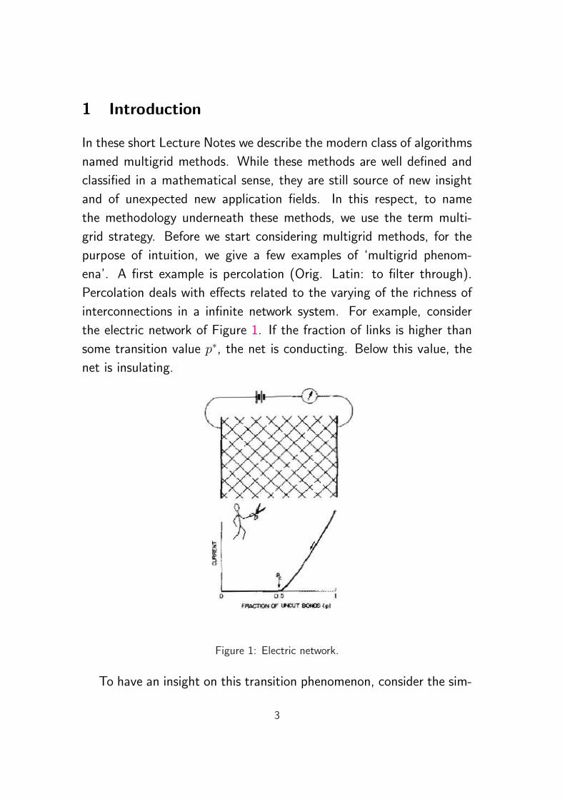
ena’. A first example is percolation (Orig. Latin: to filter through).
Percolation deals with effects related to the varying of the richness of
interconnections in a infinite network system. For example, consider
the electric network of Figure 1. If the fraction of links is higher than
some transition value p∗, the net is conducting. Below this value, the
net is insulating.
Figure 1: Electric network.
To have an insight on this transition phenomenon, consider the sim-
3

Introduction to multigrid methods 4
ple case of vertical percolation. In a 2 × 2 box there is vertical per-
colation in the cases depicted in Figure 2, which correspond to the
occurrence of a continuous dark column. Assume that a single square
in the box percolates (is dark) with probability p. Then the probability
that the 2× 2 cell percolates is
p′ = R(p) = 2p2(1− p2) + 4p3(1− p) + p4
The mapping p → R(p) has a fixed point, p∗ = R(p∗), which is the
Figure 2: Vertical percolation in a 2× 2 box.
critical value p∗ to have percolation; in our case p∗ = 0.6180. Now
define a coarsening procedure, applied to a n×n (ideally infinite) box,
which consists in replacing a 2 × 2 percolating box with a percolat-
ing square, otherwise a non percolating square. If the original box is
characterized by p < p∗, the repeated application of the coarsening
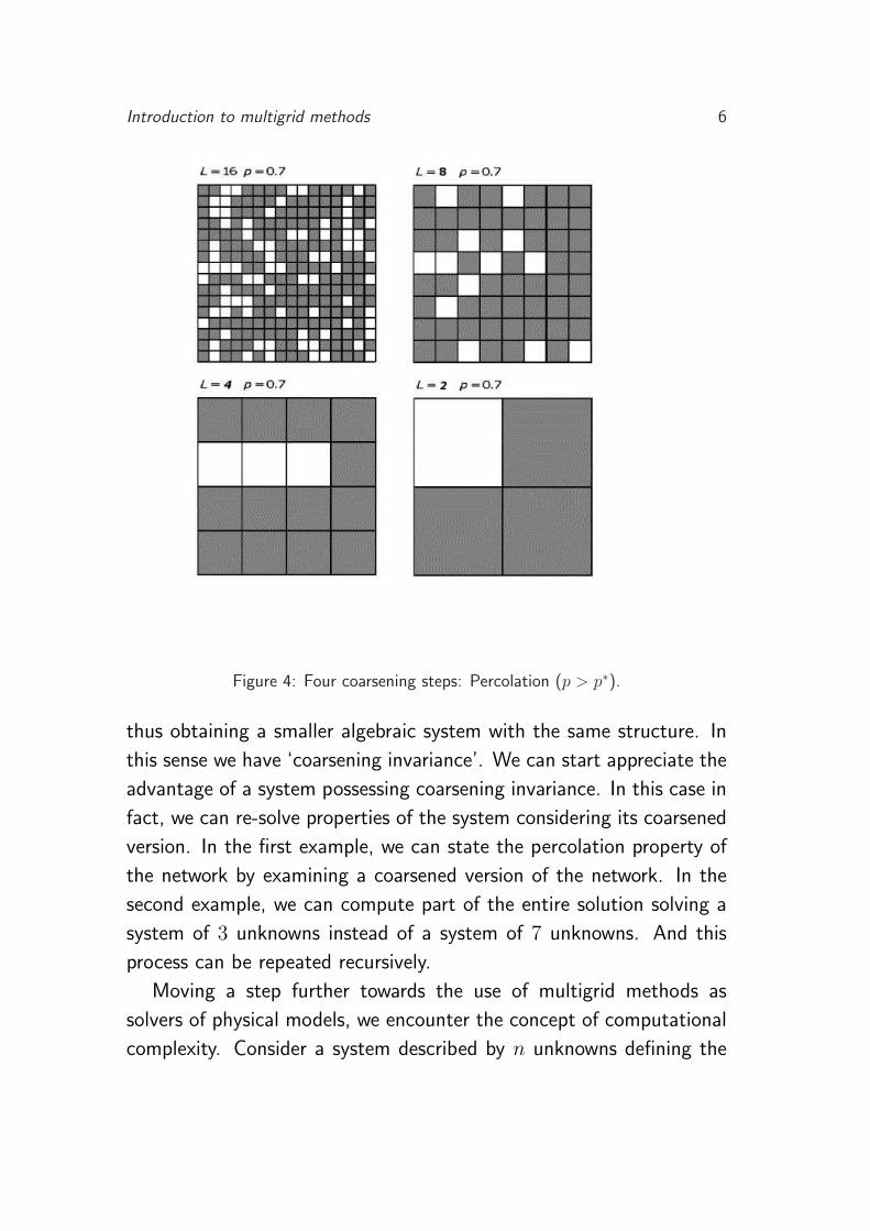
procedure results in a ‘visible’ non percolating box; see Figure 3. In the
other case of p > p∗, a repeated application of the coarsening process
reveals percolation as illustrated in Figure 4. At p = p∗ the distribution
of connections is such that we have ‘coarsening invariance’.
A second example that provides algebraic insight in the multigrid ap-
proach is cyclic reduction. Consider the finite-difference discretization
of −u′′ = f on some interval and with homogeneous Dirichlet boundary
conditions. On a uniform grid with 7 interior points the corresponding

Introduction to multigrid methods 5
Figure 3: One coarsening step: No percolation (p < p∗).
algebraic problem is given by the following linear system
E1
E2
E3
E4
E5
E6
E7
2 −1 0 0 0 0 0
−1 2 −1 0 0 0 0
0 −1 2 −1 0 0 0
0 0 −1 2 −1 0 0
0 0 0 −1 2 −1 0
0 0 0 0 −1 2 −1
0 0 0 0 0 −1 2
·
u1
u2
u3
u4
u5
u6
u7
= h2
f1
f2
f3
f4
f5
f6
f7
Let us call the equation corresponding to the row i as Ei. We define
the following coarsening steps
E ′i = R(Ei) = Ei−1 + 2 Ei + Ei+1, i = 2, 4, 6.
The result of one coarsening is
2 −1 0
−1 2 −1
0 −1 2
·
u2
u4
u6
= H2
f2
f4
f6
(H = 2h),
Introduction to multigrid methods 6
Figure 4: Four coarsening steps: Percolation (p > p∗).
thus obtaining a smaller algebraic system with the same structure. In
this sense we have ‘coarsening invariance’. We can start appreciate the
advantage of a system possessing coarsening invariance. In this case in
fact, we can re-solve properties of the system considering its coarsened
version. In the first example, we can state the percolation property of
the network by examining a coarsened version of the network. In the
second example, we can compute part of the entire solution solving a
system of 3 unknowns instead of a system of 7 unknowns. And this
process can be repeated recursively.
Moving a step further towards the use of multigrid methods as
solvers of physical models, we encounter the concept of computational
complexity. Consider a system described by n unknowns defining the
Introduction to multigrid methods 7
solution of an algebraic system. The best possible (optimal) solver is
one that provides this solution requiring a number of operations which
is linearly proportional to n. In a multigrid context this concept is some-
what refined by the following two remarks [7]: The amount of com-
putational work should be proportional to the amount of real physical
changes in the computed system; and the solution of many problems is
made of several components with different scales, which interact with
each other. Therefore, in the discretization of a continuous problem,
one should require that the number of unknowns representing the so-
lution should be proportional to the number of the physical features to
be described. So, for example, a smooth function can be represented
by a few of its values, whereas high resolution is required for highly
oscillating functions. As a consequence, to describe a solution of a
given problem the use of many scales of discretization is appropriate to
represent all components of the solution. This is one essential aspect
of the multigrid strategy.
For the purpose of this introduction we now focus on multigrid (MG)
methods for solving discretized partial differential equations and make
some historical remarks. Already in the sixties R.P. Fedorenko [15, 16]
developed the first multigrid scheme for the solution of the Poisson
equation in a unit square. Since then, other mathematicians extended
Fedorenko’s idea to general elliptic boundary value problems with vari-
able coefficients; see, e.g., [1]. However, the full efficiency of the multi-
grid approach was realized after the works of A. Brandt [3, 4] and
W. Hackbusch [18]. These Authors also introduced multigrid meth-
ods for nonlinear problems like the multigrid full approximation stor-
age (FAS) scheme [4, 21]. Another achievement in the formulation
of multigrid methods was the full multigrid (FMG) scheme [4, 21],
based on the combination of nested iteration techniques and multigrid
methods. Multigrid algorithms are now applied to a wide range of
problems, primarily to solve linear and nonlinear boundary value prob-

Introduction to multigrid methods 8
lems. Other examples of successful applications are eigenvalue problems
[6, 19], bifurcation problems [33, 37], parabolic problems [10, 20, 41],
hyperbolic problems [13, 34], and mixed elliptic/hyperbolic problems,
optimization problems [38], etc.. For additional references see, e.g.,
[23, 24, 25, 27, 32, 36, 42] and references therein. Most recent develop-
ments of solvers based on the multigrid strategy are algebraic multigrid
(AMG) methods [35] that resemble the geometric multigrid process uti-
lizing only information contained in the algebraic system to be solved.
In addition to partial differential equations (PDE), Fredholm’s integral
equations can also be efficiently solved by multigrid methods [9, 22, 26].
These schemes can be used to solve reformulated boundary value prob-
lems [21] or for the fast solution of N -body problems [2, 11]. Another
example of applications are lattice field computations and quantum
electrodynamics and chromodynamics simulations [12, 14, 17, 29, 31].
Also convergence analysis of multigrid methods has developed along
with the multitude of applications. In these Lecture Notes we only
provide introductory remarks. For results and references on MG con-
vergence theory see the Readings given below.
An essential contribution to the development of the multigrid com-
munity is the MGNet of Craig C. Douglas. This is the communication
platform on everything related to multigrid methods;
see http://www.mgnet.org.
Readings
1. J.H. Bramble, Multigrid Methods, Pitman research notes in math-
ematical series, Longman Scientific & Technical, 1993.
2. A. Brandt, Multi-grid techniques: 1984 guide with applications
to fluid dynamics, GMD-Studien. no 85, St. Augustin, Germany,
1984.
Introduction to multigrid methods 9
3. W.L. Briggs, A Multigrid Tutorial, SIAM, Philadelphia, 1987.
4. W. Hackbusch, Multi-Grid Methods and Applications, Springer-
Verlag, Heidelberg, 1985.
5. S.F. McCormick, Multigrid Methods, Frontiers in Applied Mathe-
matics, vol. 3, SIAM Books, Philadelphia, 1987.
6. U. Trottenberg, C. Oosterlee, and A. Schuller, Multigrid, Aca-
demic Press, London, 2001.
7. P. Wesseling, An introduction to multigrid methods, John Wiley,
Chichester, 1992.
2 Multigrid methods for linear problems
In this section, the basic components of a multigrid algorithm are pre-
sented. We start with the analysis of two standard iterative techniques:
the Jacobi and Gauss-Seidel schemes. These two methods are charac-
terized by global poor convergence rates, however, for errors whose
length scales are comparable to the grid mesh size, they provide rapid
damping, leaving behind smooth, longer wave-length errors. These
smooth components are responsible for the slow global convergence.
A multigrid algorithm, employing grids of different mesh sizes, allows
to solve all wave-length components and provides rapid convergence
rates. The multigrid strategy combines two complementary schemes.
The high-frequency components of the error are reduced applying itera-
tive methods like Jacobi or Gauss-Seidel schemes. For this reason these
methods are called smoothers. On the other hand, low-frequency error
components are effectively reduced by a coarse-grid correction proce-
dure. Because the action of a smoothing iteration leaves only smooth
error components, it is possible to represent them as the solution of
an appropriate coarser system. Once this coarser problem is solved, its

Introduction to multigrid methods 10
solution is interpolated back to the fine grid to correct the fine grid
approximation for its low-frequency errors.
2.1 Iterative methods and the smoothing property
Consider a large sparse linear system of equations Au = f , where A is a
n×n matrix. Iterative methods for solving this problem are formulated
as follows
u(ν+1) = Mu(ν) + Nf , (1)
where M and N have to be constructed in such a way that given an
arbitrary initial vector u(0), the sequence u(ν), ν = 0, 1, . . . , converges
to the solution u = A−1f . Defining the solution error at the sweep ν
as e(ν) = u − u(ν), iteration (1) is equivalent to e(ν+1) = Me(ν). M
is called the iteration matrix. We can state the following convergence
criterion based on the spectral radius ρ(M) of the matrix M .
Theorem 1 The method (1) converges if and only if ρ(M) < 1.
A general framework to define iterative schemes of the type (1) is
based on the concept of splitting. Assume the splitting A = B − C
where B is non singular. By setting Bu(ν+1) − Cu(ν) = f and solving
with respect to u(ν+1) one obtains
u(ν+1) = B−1Cu(ν) + B−1f .
Thus M = B−1C and N = B−1. Typically, one considers the regular
splitting A = D − L − U where D = diag(a11, a22, . . . , ann) denotes
the diagonal part of the matrix A, and −L and −U are the strictly
lower and upper parts of A, respectively. Based on this splitting many
choices for B and C are possible leading to different iterative schemes.
For example, the choice B = 1ωD and C = 1
ω [(1− ω)D + ω(L + U)],
0 < ω ≤ 1, leads to the damped Jacobi iteration
u(ν+1) = (I − ωD−1A)u(ν) + ωD−1f . (2)

Introduction to multigrid methods 11
Choosing B = D − L and C = U , one obtains the Gauss-Seidel
iteration
u(ν+1) = (D − L)−1Uu(ν) + (D − L)−1f . (3)
Later on we denote the iteration matrices corresponding to (2) and (3)
with MJ(ω) and MGS, respectively.
To define and analyze the smoothing property of these iterations
we introduce a simple model problem. Consider the finite-difference
approximation of a one-dimensional Dirichlet boundary value problem:
−d2u
dx2 = f(x), in Ω = (0, 1)
u(x) = g(x), on x ∈ 0, 1 .(4)
Let Ω be represented by a grid Ωh with grid size h = 1n+1 and grid points
xj = jh, j = 0, 1, . . . , n + 1. A discretization scheme for the second
derivative at xj is h−2[u(xj−1)− 2u(xj) + u(xj+1)] = u′′(xj) + O(h2).
Set fhj = f(jh), and uh
j = u(jh). We obtain the following tridiagonal
system of n equations
2
h2 uh1 −
1
h2 uh2 = fh
1 +1
h2 g(0)
− 1
h2 uhj−1 +
2
h2 uhj −
1
h2 uhj+1 = fh
j , j = 2, . . . , n− 1 (5)
− 1
h2 uhn−1 +
2
h2 uhn = fh
n +1
h2 g(1)
Let us omit the discretization parameter h and denote (5) by Au = f .
We discuss the solution to this problem by using the Jacobi iteration.
Consider the eigenvalue problem for the damped Jacobi iteration, given
by MJ(ω)vk = µkvk. The eigenvectors are given by
vk = (sin(kπhj))j=1,n , k = 1, . . . , n , (6)
and the corresponding eigenvalues are
µk(ω) = 1− ω(1− cos(kπh)) , k = 1, . . . , n . (7)

Introduction to multigrid methods 12
We have that ρ(MJ(ω)) < 1 for 0 < ω ≤ 1, guaranteeing convergence.
In particular, for the Jacobi iteration with ω = 1 we have ρ(MJ(1)) =
1− 12πh2+O(h4), showing how the convergence of (2) deteriorates (i.e.
ρ tends to 1) as h → 0. However, the purpose of an iteration in a MG
algorithm is primarily to be a smoothing operator. In order to define
this property, we need to distinguish between low- and high-frequency
eigenvectors. We define
• low frequency (LF) vk with 1 ≤ k < n2 ;
• high frequency (HF) vk with n2 ≤ k ≤ n;
We now define the smoothing factor µ as the worst factor by which
the amplitudes of HF components are damped per iteration. In the
case of the Jacobi iteration we have
µ = max|µk|, n
2≤ k ≤ n = max1− ω, |1− ω(1− cos(π)|
≤ max1− ω, |1− 2ω|.Using this result we find that the optimal smoothing factor µ = 1/3 is
obtained choosing ω∗ = 2/3.
Now suppose to apply ν times the damped Jacobi iteration with ω =
ω∗. Consider the following representation of the error e(ν) =∑
k e(ν)k vk.
The application of ν-times the damped Jacobi iteration on the initial
error e(0) results in e(ν) = MJ(ω∗)νe(0). This implies for the expansion
coefficients that e(ν)k = µk(ω
∗)νe(0)k . Therefore a few sweeps of (2)
give |e(ν)k | << |e(0)
k | for high-frequency components. For this reason,
although the global error decreases slowly by iteration, it is smoothed
very quickly and this process does not depend on h.
Most often, instead of a Jacobi method other iterations are used
that suppress the HF components of the error more efficiently. This is
the case, for example, of the Gauss-Seidel iteration (3). The smoothing
property of this scheme is conveniently analyzed by using local mode
analysis (LMA) introduced by Brandt [4]. This is an effective tool for

Introduction to multigrid methods 13
analyzing the MG process even though it is based on certain idealized
assumptions and simplifications: Boundary conditions are neglected and
the problem is considered on infinite grids Gh = jh, j ∈ Z. Notice
that on Gh, only the components eiθx/h with θ ∈ (−π, π] are visible,
i.e., there is no other component with frequency θ0 ∈ (−π, π] with
|θ0| < θ such that eiθ0x/h = eiθx/h, x ∈ Gh.
In LMA the notion of low- and high-frequency components on the
grid Gh is related to a coarser grid denoted by GH . In this way eiθx/h
on Gh is said to be an high-frequency component, with respect to the
coarse grid GH , if its restriction (projection) to GH is not visible there.
Usually H = 2h and the high frequencies are those with π2 ≤ |θ| ≤ π.
We give an example of local mode analysis considering the Gauss-
Seidel scheme applied to our discretized model problem. A relaxation
sweep starting from an initial approximation u(ν) produces a new ap-
proximation u(ν+1) such that the corresponding error satisfies
Bhe(ν+1)(x)− Che
(ν)(x) = 0 , x ∈ Gh , (8)
where Bh = Dh−Lh and Ch = Uh. To analyze this iteration we define
the errors in terms of their θ components e(ν) =∑
θ E (ν)θ eiθx/h and
e(ν+1) =∑
θ E (ν+1)θ eiθx/h. Where E (ν)
θ and E (ν+1)θ denote the error am-
plitudes of the θ component, before and after smoothing, respectively.
Then, for a given θ, (8) reduces to
(2− e−iθ)E (ν+1)θ − eiθE (ν)
θ = 0 .
In the LMA framework, the smoothing factor is defined by
µ = max|E(ν+1)θ
E (ν)θ
| ,π
2≤ |θ| ≤ π , (9)
For the present model problem we obtain
|E(ν+1)θ
E (ν)θ
| = | eiθ
2− e−iθ|,

Introduction to multigrid methods 14
and µ = 0.45. Similar values are obtained by LMA for the Gauss-Seidel
iteration applied to the two- and three-dimensional version of our model
problem. For the two dimensional case the effect of smoothing can be
seen in Figure 5.
010
2030
0
20
40−1
0
1
Initial error, Physical Space
010
2030
0
20
40−1
0
1
Physical Space, 1 iter(s), Gauss−Seidel.
010
2030
0
20
40−0.5
0
0.5
Physical Space, 2 iter(s), Gauss−Seidel.
010
2030
0
20
40−0.5
0
0.5
Physical Space, 3 iter(s), Gauss−Seidel.
Figure 5: Smoothing by Gauss-Seidel iteration.
Another definition of smoothing property of an iterative scheme is
due to Hackbusch [21]. Let M be the iteration matrix of a smoothing
procedure and recall the relation e(ν) = M νe(0). One can measure the
smoothness of e(ν) by a norm involving differences of the value of this
error on different grid points. A natural choice is to take the second-
order difference matrix Ah above. Then the following smoothing factor
is defined
µ(ν) = ‖AhMν‖/‖Ah‖. (10)
Introduction to multigrid methods 15
The iteration defined by M is said to possess the smoothing property if
there exists a function η(ν) such that, for sufficiently large ν, we have
‖AhMν‖ ≤ η(ν)/hα,
where α > 0 and η(ν) → 0 as ν → ∞. For our model problem using
the damped Jacobi iteration, α = 2 and η(ν) = νν/(ν + 1)(ν+1). For
the Gauss-Seidel iteration we have α = 2 and η(ν) = c/ν with c a
positive constant.
2.2 The twogrid scheme and the approximation property
After the application of a few smoothing sweeps, we obtain an ap-
proximation uh whose error eh = uh − uh is smooth. Then eh can be
approximated on a coarser space. We need to express this smooth error
as solution of a coarse problem, whose matrix AH and right-hand side
have to be defined. For this purpose notice that in our model problem,
Ah is a second-order difference operator and the residual rh = fh−Ahuh
is a smooth function if eh is smooth. Obviously the original equation
Ahuh = fh and the residual equation Aheh = rh are equivalent. The
difference is that eh and rh are smooth, therefore we can think of rep-
resenting them on a coarser grid with mesh size H = 2h. We define
rH as the restriction of the fine-grid residual to the coarse grid, that is,
rH = IHh rh, where IH
h is a suitable restriction operator (for example, in-
jection). This defines the right-hand side of the coarse problem. Since
eh is the solution of a difference operator which can be represented
analogously on the coarse discretization level, we define the following
coarse problem
AH eH = rH , (11)
with homogeneous Dirichlet boundary conditions as for eh. Here AH
represents the same discrete operator but relative to the grid with mesh
size H. Reasonably one expects that eH be an approximation to eh on
Introduction to multigrid methods 16
the coarse grid. Because of its smoothness, we can apply a prolon-
gation operator IhH to transfer eH to the fine grid. Therefore, since
by definition uh = uh + eh, we update the function uh applying the
following coarse-grid correction (CGC) step
unewh = uh + Ih
H eH .
Notice that eh was a smooth function and the last step has amended
uh by its smooth error. In practice, also the interpolation procedure
may introduce HF errors on the fine grid. Therefore it is convenient
to complete the twogrid process by applying ν2 post-smoothing sweeps
after the coarse-grid correction.
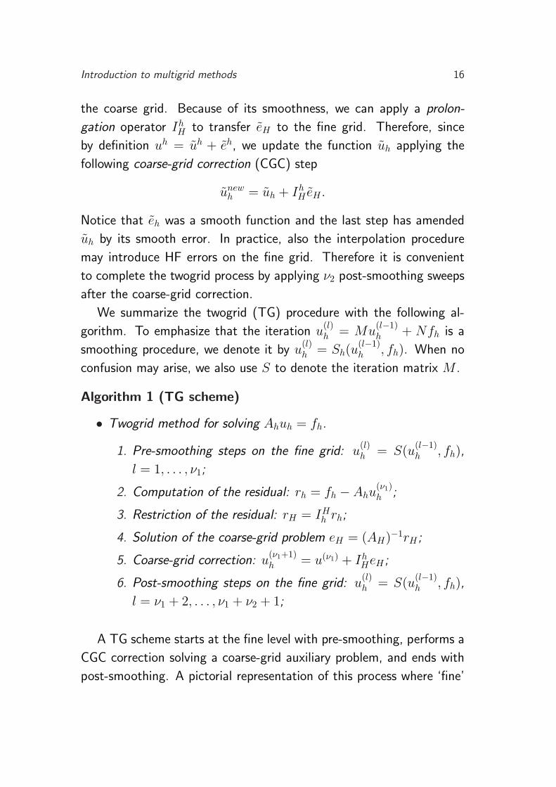
We summarize the twogrid (TG) procedure with the following al-
gorithm. To emphasize that the iteration u(l)h = Mu
(l−1)h + Nfh is a
smoothing procedure, we denote it by u(l)h = Sh(u
(l−1)h , fh). When no
confusion may arise, we also use S to denote the iteration matrix M .
Algorithm 1 (TG scheme)
• Twogrid method for solving Ahuh = fh.
1. Pre-smoothing steps on the fine grid: u(l)h = S(u
(l−1)h , fh),
l = 1, . . . , ν1;
2. Computation of the residual: rh = fh − Ahu(ν1)h ;
3. Restriction of the residual: rH = IHh rh;
4. Solution of the coarse-grid problem eH = (AH)−1rH ;
5. Coarse-grid correction: u(ν1+1)h = u(ν1) + Ih
HeH ;
6. Post-smoothing steps on the fine grid: u(l)h = S(u
(l−1)h , fh),
l = ν1 + 2, . . . , ν1 + ν2 + 1;
A TG scheme starts at the fine level with pre-smoothing, performs a
CGC correction solving a coarse-grid auxiliary problem, and ends with
post-smoothing. A pictorial representation of this process where ‘fine’
Introduction to multigrid methods 17
is a high level and ‘coarse’ is a low level looks like a ‘V’ workflow. This
is called V cycle. To solve the problem to a given tolerance, we have to
apply the TG V-cycle repeatedly (iteratively). Actually, the TG scheme
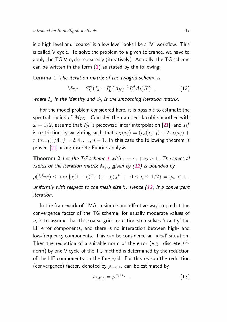
can be written in the form (1) as stated by the following
Lemma 1 The iteration matrix of the twogrid scheme is
MTG = Sν2
h (Ih − IhH(AH)−1IH
h Ah)Sν1
h , (12)
where Ih is the identity and Sh is the smoothing iteration matrix.
For the model problem considered here, it is possible to estimate the
spectral radius of MTG. Consider the damped Jacobi smoother with
ω = 1/2, assume that IhH is piecewise linear interpolation [21], and IH
h
is restriction by weighting such that rH(xj) = (rh(xj−1) + 2 rh(xj) +
rh(xj+1))/4, j = 2, 4, . . . , n− 1. In this case the following theorem is
proved [21] using discrete Fourier analysis
Theorem 2 Let the TG scheme 1 with ν = ν1 + ν2 ≥ 1. The spectral
radius of the iteration matrix MTG given by (12) is bounded by
ρ(MTG) ≤ maxχ(1−χ)ν +(1−χ)χν : 0 ≤ χ ≤ 1/2 =: ρν < 1 ,
uniformly with respect to the mesh size h. Hence (12) is a convergent
iteration.
In the framework of LMA, a simple and effective way to predict the
convergence factor of the TG scheme, for usually moderate values of
ν, is to assume that the coarse-grid correction step solves ‘exactly’ the
LF error components, and there is no interaction between high- and
low-frequency components. This can be considered an ‘ideal’ situation.
Then the reduction of a suitable norm of the error (e.g., discrete L2-
norm) by one V cycle of the TG method is determined by the reduction
of the HF components on the fine grid. For this reason the reduction
(convergence) factor, denoted by ρLMA, can be estimated by
ρLMA = µν1+ν2 . (13)

Introduction to multigrid methods 18
A sharper bound can be computed by twogrid local mode analysis [8].
In Table 1, we report estimates of ρLMA as given by (13) and estimates
of ρν by Theorem 2. Notice that the estimate ρLMA approximates well
the bound ρν provided that ν1 + ν2 is small. For large ν, ρLMA has an
exponential behavior whereas ρν ' 1/eν.
ν ρLMA ρν
1 0.5 0.5
2 0.25 0.25
3 0.125 0.125
4 0.0625 0.0832
5 0.03125 0.0671
Table 1: Comparison of error reduction factors as given by LMA and by Theorem 2.
Notice that measuring ρ requires the knowledge of the exact so-
lution. Because this is usually not available, ρ is measured as the
asymptotic value of the reduction of a suitable norm of the residuals
after consecutive TG cycles.
Together with the definition of the smoothing property (10), Hack-
busch introduces the approximation property to measure how good the
coarse-grid solution approximates the fine grid solution. This is ex-
pressed by the following estimate
‖A−1h − Ih
H A−1H IH
h ‖ ≤ cA hβ. (14)
Notice that this estimate actually measures the accuracy between uh =
A−1h fh and Ih
HuH where uH = A−1H IH
h fh.
In our model problem we have β = 2. Using the estimates of the
smoothing and approximation properties, one can prove convergence of
the TG scheme as follows. Consider, for simplicity, ν2 = 0, i.e. only

Introduction to multigrid methods 19
pre-smoothing is applied. Then for our model problem we have
‖MTG‖ = ‖(Ih − IhH(AH)−1IH
h Ah)Sν1
h ‖= ‖(A−1
h − IhH(AH)−1IH
h )AhSν1
h ‖≤ ‖A−1
h − IhH(AH)−1IH
h ‖‖AhSν1
h ‖≤ cA η(ν1), (15)
where cA η(ν1) < 1 for sufficiently large ν1. Notice that the coarse-
grid correction without pre- and post-smoothing is not a convergent
iteration, in general. In fact, IHh maps from a fine- to a coarse-
dimensional space and IhH(AH)−1IH
h is not invertible. We have ρ(Ih −IhH(AH)−1IH
h Ah) ≥ 1.
2.3 The multigrid scheme
In the TG scheme the size of the coarse grid is twice larger than the fine
one, thus the coarse problem may be very large. However, the coarse
problem has the same form as the residual problem on the fine level.
Therefore one can use the TG method to determine eH , i.e. equation
(11) is itself solved by TG cycling introducing a further coarse-grid
problem. This process can be repeated recursively until a coarsest grid
is reached where the corresponding residual equation is inexpensive
to solve. This is, roughly speaking, the qualitative description of the
multigrid method.
For a more detailed description, let us introduce a sequence of grids
with mesh size h1 > h2 > · · · > hL > 0, so that hk−1 = 2 hk. Here
k = 1, 2, . . . , L, is called the level number. With Ωhkwe denote the set
of grid points with grid spacing hk. The number of interior grid points
will be nk.
On each level k we define the problem Akuk = fk. Here Ak is a
nk × nk matrix, and uk, fk are vectors of size nk. The transfer among
levels is performed by two linear mappings. The restriction Ik−1k and

Introduction to multigrid methods 20
the prolongation Ikk−1 operators. With uk = Sk(uk, fk) we denote a
smoothing iteration. The following defines the multigrid algorithm
Algorithm 2 (MG scheme)
• Multigrid method for solving Akuk = fk.
1. If k = 1 solve Akuk = fk directly.
2. Pre-smoothing steps on the fine grid: u(l)k = S(u
(l−1)k , fk),
l = 1, . . . , ν1;
3. Computation of the residual: rk = fk − Aku(ν1)k ;
4. Restriction of the residual: rk−1 = Ik−1k rk;
5. Set uk−1 = 0;
6. Call γ times the MG scheme to solve Ak−1uk−1 = rk−1;
7. Coarse-grid correction: u(ν1+1)k = u
(ν1)k + Ik
k−1uk−1;
8. Post-smoothing steps on the fine grid: u(l)k = S(u
(l−1)k , fk),
l = ν1 + 2, . . . , ν1 + ν2 + 1;
The multigrid algorithm involves a new parameter (cycle index) γ
which is the number of times the MG procedure is applied to the coarse
level problem. Since this procedure converges very fast, γ = 1 or γ = 2
are the typical values used. For γ = 1 the multigrid scheme is called
V-cycle, whereas γ = 2 is named W-cycle. It turns out that with a
reasonable γ, the coarse problem is solved almost exactly. Therefore in
this case the convergence factor of a multigrid cycle equals that of the
corresponding TG method, i.e., approximately ρ = µν1+ν2. Actually in
many problems γ = 2 or even γ = 1 are sufficient to retain the twogrid
convergence.
Also the multigrid scheme can be expressed in the form (1) as stated
by the following lemma
Introduction to multigrid methods 21
Lemma 2 The iteration matrix of the multigrid scheme is given in
recursive form by the following.
For k = 1 let M1 = 0. For k = 2, . . . , L:
Mk = Sν2
k (Ik − Ikk−1(Ik−1 −Mγ
k−1)A−1k−1I
k−1k Ak)S
ν1
k (16)
where Ik is the identity, Sk is the smoothing iteration matrix, and Mk
is the multigrid iteration matrix for the level k.
To derive (16) consider an initial error e(0)k . The action of ν1 pre-
smoothing steps gives ek = Sν1
k e(0)k and the corresponding residual rk =
Akek. On the coarse grid, this error is given by ek−1 = A−1k−1I
k−1k rk.
However, in the multigrid algorithm we do not invert Ak−1 (unless
on the coarsest grid) and we apply γ multigrid cycles instead. That is,
denote with v(γ)k−1 the approximation to ek−1 obtained after γ application
of Mk−1, we have
ek−1 − v(γ)k−1 = M
(γ)k−1(ek−1 − v
(0)k−1).
Following the MG Algorithm 2, we set v(0)k−1 = 0 (Step 5.). Therefore
we have ek−1 − v(γ)k−1 = M
(γ)k−1ek−1 which can be rewritten as v
(γ)k−1 =
(Ik−1 −M(γ)k−1)ek−1. It follows that
v(γ)k−1 = (Ik−1 −M
(γ)k−1)ek−1 = (Ik−1 −M
(γ)k−1) A−1
k−1Ik−1k rk
= (Ik−1 −M(γ)k−1) A−1
k−1Ik−1k Akek.
Correspondingly, the coarse-grid correction is u(ν1+1)k = u
(ν1)k +Ik
k−1v(γ)k−1.
In terms of error functions this means that
e(ν1+1)k = ek − Ik
k−1v(γ)k−1,
substituting the expression for v(γ)k−1 given above, we obtain
e(ν1+1)k = [Ik − Ik
k−1(Ik−1 −M(γ)k−1) A−1
k−1Ik−1k Ak]ek.
Finally, consideration of the pre- and post-smoothing sweeps proves the
Lemma.
A picture of the multigrid workflow is given in Figure 6.

Introduction to multigrid methods 22
Figure 6: Multigrid setting.
3 Multigrid methods for nonlinear problems
Many problems of physical interest are nonlinear in character and for
these problems the multigrid strategy provides new powerful algorithms.
Roughly speaking there are two multigrid approaches to nonlinear prob-
lems. The first is based on the generalization of the MG scheme de-
scribed above. The second is based on the Newton method and uses
the multigrid scheme as inner solver of the linearized equations. In this
respect the latter approach does not belong, conceptually, to the class
of multigrid methods. The well known representative of the former
approach is the full approximation storage (FAS) scheme [4].
An interesting comparison between the FAS and the MG-Newton
schemes is presented in [28]. First, it is shown that, in terms of com-
puting time, the exact Newton approach is not a viable method. In the
case of multigrid-inexact-Newton scheme it is shown that this approach
may have similar efficiency as the FAS scheme. However, it remains
an open issue how many interior MG cycles are possibly needed in the
MG-Newton method to match the FAS efficiency. In this sense the FAS
scheme is more robust and we discuss this method in the following.
Introduction to multigrid methods 23
In the FAS scheme the global linearization in the Newton process
is avoided and the only possible linearization involved is a local one in
order to define the relaxation procedure, e.g., Gauss-Seidel-Newton. To
illustrate the FAS method, consider the nonlinear problem A(u) = f ,
and denote its discretization by
Ak(uk) = fk , (17)
where Ak(·) represents a nonlinear discrete operator on Ωhk.
The starting point for the FAS scheme is again to define a suitable
smoothing iteration. We denote the corresponding smoothing process
by u = S (u, f). Now suppose to apply a few times this iterative
method to (17) obtaining some approximate solution uk. The desired
exact correction ek is defined by Ak(uk + ek) = fk. Here the coarse
residual equation (11) makes no sense (no superposition). Nevertheless
the ‘correction’ equation can instead be written in the form
Ak(uk + ek)− Ak(uk) = rk , (18)
if we define rk = fk − Ak(uk). Assume to represent uk + ek on the
coarse grid in terms of the coarse-grid variable
uk−1 := Ik−1k uk + ek−1 . (19)
Since Ik−1k uk and uk represent the same function but on different grids,
the standard choice of the fine-to-coarse linear operator Ik−1k is the
straight injection. Formulating (18) on the coarse level by replacing
Ak(·) by Ak−1(·), uk by Ik−1k uk, and rk by Ik−1
k rk = Ik−1k (fk−Ak(uk)),
we get the FAS equation
Ak−1(uk−1) = Ik−1k (fk − Ak(uk)) + Ak−1(I
k−1k uk) . (20)
This equation is also written in the form
Ak−1(uk−1) = Ik−1k fk + τ k−1
k , (21)
Introduction to multigrid methods 24
where
τ k−1k = Ak−1(I
k−1k uk)− Ik−1
k Ak(uk).
Observe that (21) without the τ k−1k term is the original equation rep-
resented on the coarse grid. At convergence uk−1 = Ik−1k uk, because
fk − Ak(uk) = 0 and Ak−1(uk−1) = Ak−1(Ik−1k uk). The term τ k−1
k is
the fine-to-coarse defect or residual correction. That is, the correction
to (21) such that its solution coincides with the fine grid solution. This
fact allows to reverse the point of view of the multigrid approach [7].
Instead of regarding the coarse level as a device for accelerating con-
vergence on the fine grid, one can view the fine grid as a device for
calculating the correction τ k−1k to the FAS equation. In this way most
of the calculation may proceed on coarser spaces.
The direct use of uk−1 on fine grids, that is, the direct interpolation
of this function by Ikk−1uk−1 cannot be used, since it introduces the
interpolation errors of the full (possibly oscillatory) solution, instead of
the interpolation errors of only the correction ek−1, which in principle
is smooth because of the application of the smoothing iteration. For
this reason the following coarse-grid correction is used
uk = uk + Ikk−1(uk−1 − Ik−1
k uk) . (22)
The complete FAS scheme is summarized below
Algorithm 3 (FAS scheme)
• Multigrid FAS method for solving Ak(uk) = fk.
1. If k = 1 solve Ak(uk) = fk directly.
2. Pre-smoothing steps on the fine grid: u(l)k = S(u
(l−1)k , fk),
l = 1, . . . , ν1;
3. Computation of the residual: rk = fk − Aku(ν1)k ;
4. Restriction of the residual: rk−1 = Ik−1k rk;
5. Set uk−1 = Ik−1k u
(ν1)k ;
Introduction to multigrid methods 25
6. Set fk−1 = rk−1 + Ak−1(uk−1)
7. Call γ times the FAS scheme to solve Ak−1(uk−1) = fk−1;
8. Coarse-grid correction: u(ν1+1)k = u
(ν1)k +Ik
k−1(uk−1−Ik−1k u
(ν1)k );
9. Post-smoothing steps on the fine grid: u(l)k = S(u
(l−1)k , fk),
l = ν1 + 2, . . . , ν1 + ν2 + 1;
4 The full multigrid method
When dealing with nonlinear problems it is sometimes important to
start the iterative procedure from a good initial approximation. The
multigrid setting suggests a natural way of how to get this approxi-
mation cheaply. Suppose to start the solution process from a coarse
working level (present fine grid) ` < M where the discretized problem
A`(u`) = f` is easily solved. We can usually interpolate this solution
to the next finer working level as initial approximation for the iterative
process to solve A`+1(u`+1) = f`+1. We apply the interpolation
u`+1 = I`+1` u` , (23)
and then start the FAS (or MG) solution process at level `+1. The idea
of using a coarse-grid approximation as a first guess for the solution
process on a finer grid is known as nested iteration. The algorithm
obtained by combining the multigrid scheme with nested iteration is
called full multigrid (FMG) method; see Figure 7. The interpolation
operator (23) used in the FMG scheme is called FMG interpolator.
Because of the improvement on the initial solution at each starting level,
the FMG scheme results to be cheaper than the iterative application of
the multigrid cycle without FMG initialization.
Algorithm 4 (FMG scheme)
• FMG method for solving AL(uL) = fL.
Introduction to multigrid methods 26
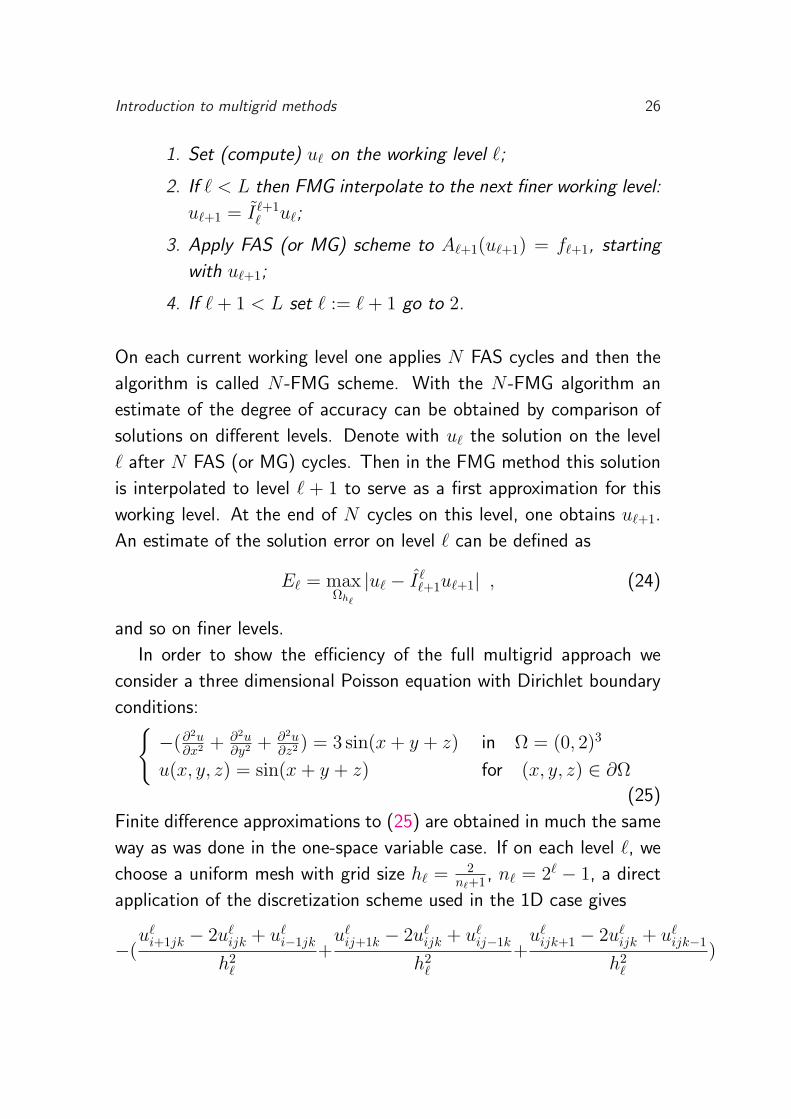
1. Set (compute) u` on the working level `;
2. If ` < L then FMG interpolate to the next finer working level:
u`+1 = I`+1` u`;
3. Apply FAS (or MG) scheme to A`+1(u`+1) = f`+1, starting
with u`+1;
4. If ` + 1 < L set ` := ` + 1 go to 2.
On each current working level one applies N FAS cycles and then the
algorithm is called N -FMG scheme. With the N -FMG algorithm an
estimate of the degree of accuracy can be obtained by comparison of
solutions on different levels. Denote with u` the solution on the level
` after N FAS (or MG) cycles. Then in the FMG method this solution
is interpolated to level ` + 1 to serve as a first approximation for this
working level. At the end of N cycles on this level, one obtains u`+1.
An estimate of the solution error on level ` can be defined as
E` = maxΩh`
|u` − I``+1u`+1| , (24)
and so on finer levels.
In order to show the efficiency of the full multigrid approach we
consider a three dimensional Poisson equation with Dirichlet boundary
conditions:−(∂2u
∂x2 + ∂2u∂y2 + ∂2u
∂z2 ) = 3 sin(x + y + z) in Ω = (0, 2)3
u(x, y, z) = sin(x + y + z) for (x, y, z) ∈ ∂Ω
(25)
Finite difference approximations to (25) are obtained in much the same
way as was done in the one-space variable case. If on each level `, we
choose a uniform mesh with grid size h` = 2n`+1 , n` = 2` − 1, a direct
application of the discretization scheme used in the 1D case gives
−(u`
i+1jk − 2u`ijk + u`
i−1jk
h2`
+u`
ij+1k − 2u`ijk + u`
ij−1k
h2`
+u`
ijk+1 − 2u`ijk + u`
ijk−1
h2`
)

Introduction to multigrid methods 27
= 3 sin(ih`, jh`, kh`) , i, j, k = 1, . . . , n` . (26)
This is the 7-point stencil approximation which is O(h2) accurate. To
solve this problem we employ the FAS scheme with γ = 1 and L =
7. The smoothing iteration is the lexicographic Gauss-Seidel method,
applied ν1 = 2 times for pre-smoothing and ν2 = 1 times as post-
smoother. Its smoothing factor estimated by local mode analysis is
µ = 0.567. Hence, by this analysis, the expected reduction factor is
ρ∗ = µν1+ν2 = 0.18. The observed reduction factor is ≈ 0.20.
Here Ik−1k is simple injection and Ik−1
k and Ikk−1 are the full weighting
and (tri-)linear interpolation, respectively. Finally, the FMG operator
I`+1` is cubic interpolation [7, 21]. Now let us discuss the optimality of
the FMG algorithm constructed with these components.
To show that the FMG scheme is able to solve the given discrete
problem at a minimal cost, we compute E` and show that it behaves
like h2` , demonstrating convergence. This means that the ratio E`/E`+1
at convergence should be a factor h2`/h
2`+1 = 4. Results are reported in
Table 2. In the 10-FMG column of we actually observe the h2 behavior
which can also be seen with smaller N = 3 and N = 1 FMG schemes.
` = 1
` = 2
` = 3
µ´¶³
AAAAU
µ´¶³¢
¢¢¢µ´¶³
AAAAU
µ´¶³
AAAAU
µ´¶³¢
¢¢¢µ´¶³¢
¢¢¢µ´¶³
AAAAU
µ´¶³
AAAAU
µ´¶³
ν
ν1
ν
ν2
ν1
ν1
ν
ν2
ν2
Figure 7: The FMG scheme.

Introduction to multigrid methods 28
In fact, as reported in Table 2, the 1-FMG scheme gives the same order
of magnitude of errors as the 10-FMG scheme. Therefore the choice
N = 1 in a FMG cycle is suitable to solve the problem to second-order
accuracy.
level 10-FMG 3-FMG 1-FMG
3 6.75 10−4 6.79 10−4 9.44× 10⁻⁴
4 1.73 10−4 1.75 10−4 2.34× 10⁻⁴
5 4.36 10−5 4.40 10−5 5.92× 10⁻⁵
6 1.09 10−5 1.10 10−5 1.48× 10⁻⁵
Table 2: The estimated solution error for various N -FMG cycles.
To estimate the amount of work invested in the FMG method, let
us define the work unit (WU) [4], i.e. the computational work of one
smoothing sweep on the finest level M . The number of corresponding
arithmetic operations is linearly proportional to the number of grid
points. On the level ` ≤ M the work involved is (12)
3(M−`)WU , where
the factor 12 is given by the mesh size ratio h`+1/h` and the exponent 3
is the number of spatial dimensions. Thus a multigrid cycle that uses
ν = ν1 + ν2 relaxation sweeps on each level requires
Wcycle = ν
L∑
k=1
(1
2)3(L−k)WU <
8
7νWU ,
ignoring transfer operations. Hence the computational work employed
in a N -FMG method is roughly
WFMG = NL∑
`=2
(1
2)3(L−`)Wcycle ,
ignoring the FMG interpolation and work on the coarsest grid. This
means that, using the 1-FMG method, we solve the discrete 3D Poisson
problem to second-order accuracy with a number of computer opera-
tions which is proportional to the number of unknowns on the finest
grid. In the present case we have FMG Work ≈ 4WU .
Introduction to multigrid methods 29
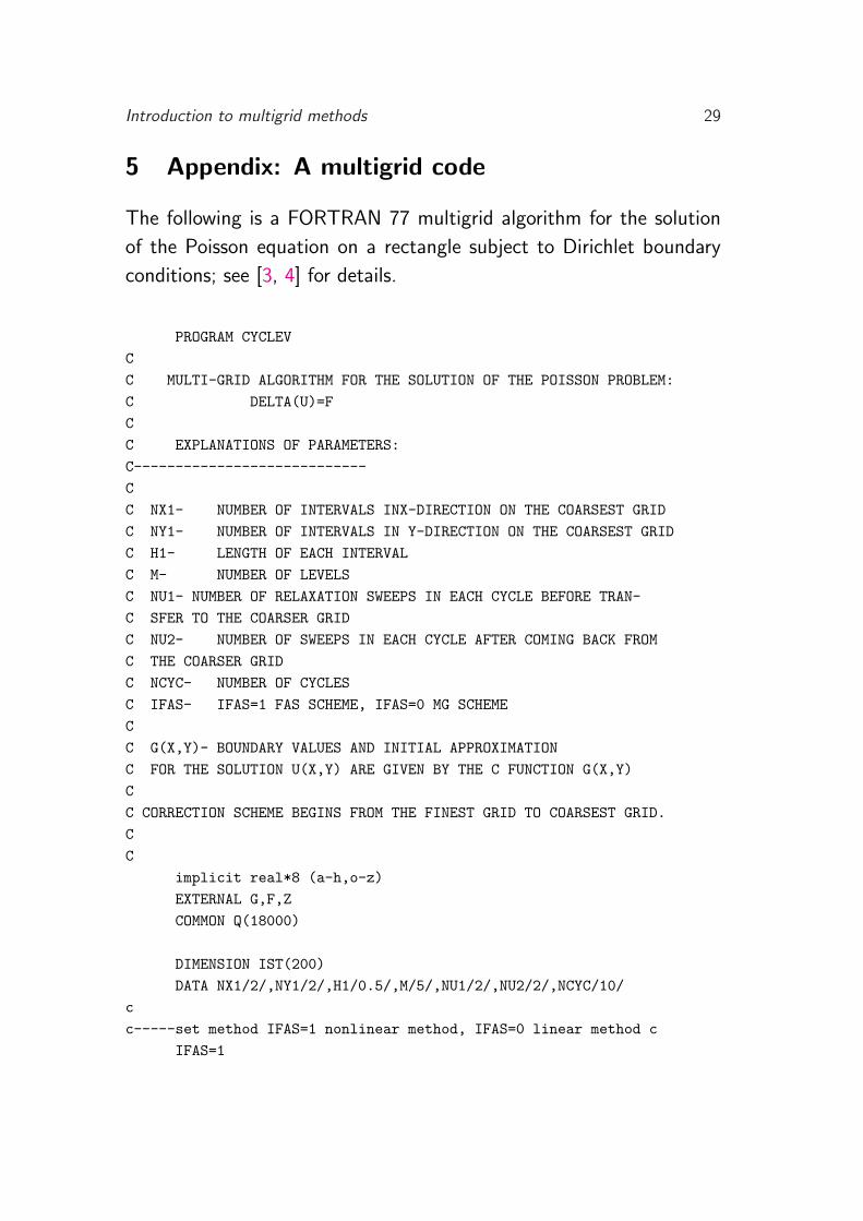
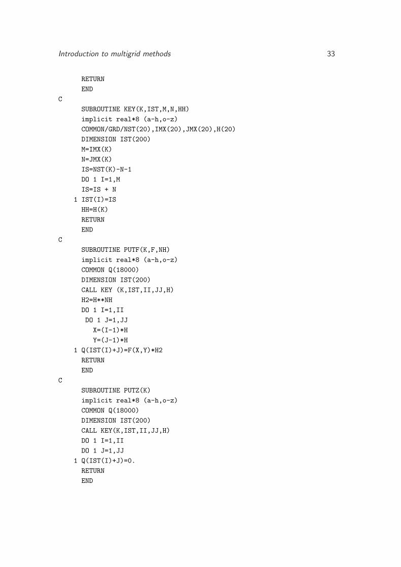
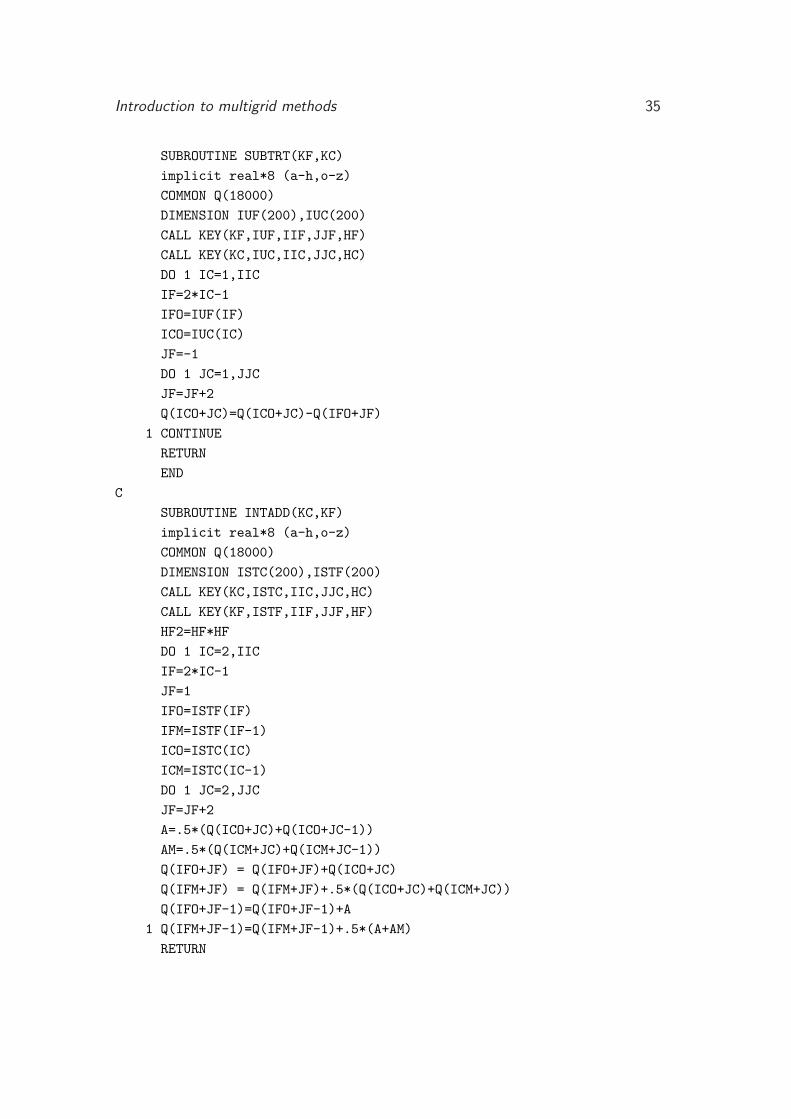
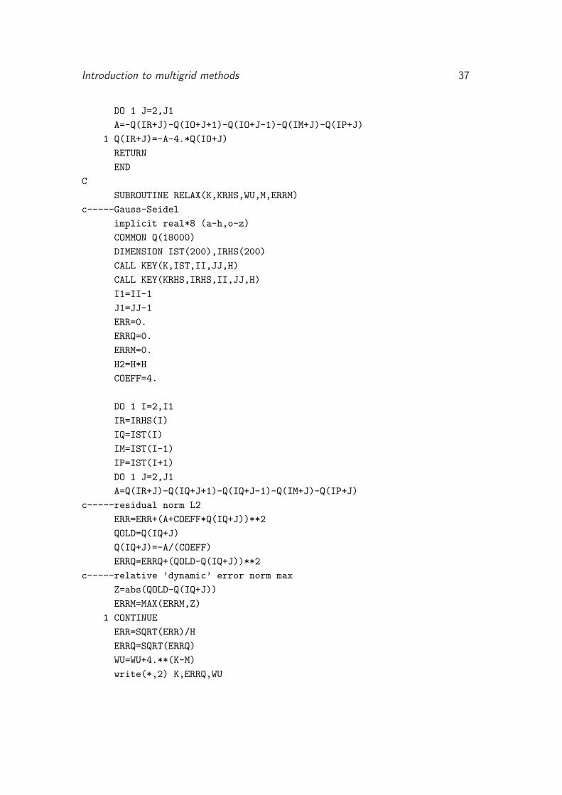
5 Appendix: A multigrid code
The following is a FORTRAN 77 multigrid algorithm for the solution
of the Poisson equation on a rectangle subject to Dirichlet boundary
conditions; see [3, 4] for details.
PROGRAM CYCLEV
C
C MULTI-GRID ALGORITHM FOR THE SOLUTION OF THE POISSON PROBLEM:
C DELTA(U)=F
C
C EXPLANATIONS OF PARAMETERS:
C----------------------------
C
C NX1- NUMBER OF INTERVALS INX-DIRECTION ON THE COARSEST GRID
C NY1- NUMBER OF INTERVALS IN Y-DIRECTION ON THE COARSEST GRID
C H1- LENGTH OF EACH INTERVAL
C M- NUMBER OF LEVELS
C NU1- NUMBER OF RELAXATION SWEEPS IN EACH CYCLE BEFORE TRAN-
C SFER TO THE COARSER GRID
C NU2- NUMBER OF SWEEPS IN EACH CYCLE AFTER COMING BACK FROM
C THE COARSER GRID
C NCYC- NUMBER OF CYCLES
C IFAS- IFAS=1 FAS SCHEME, IFAS=0 MG SCHEME
C
C G(X,Y)- BOUNDARY VALUES AND INITIAL APPROXIMATION
C FOR THE SOLUTION U(X,Y) ARE GIVEN BY THE C FUNCTION G(X,Y)
C
C CORRECTION SCHEME BEGINS FROM THE FINEST GRID TO COARSEST GRID.
C
C
implicit real*8 (a-h,o-z)
EXTERNAL G,F,Z
COMMON Q(18000)
DIMENSION IST(200)
DATA NX1/2/,NY1/2/,H1/0.5/,M/5/,NU1/2/,NU2/2/,NCYC/10/
c
c-----set method IFAS=1 nonlinear method, IFAS=0 linear method c
IFAS=1
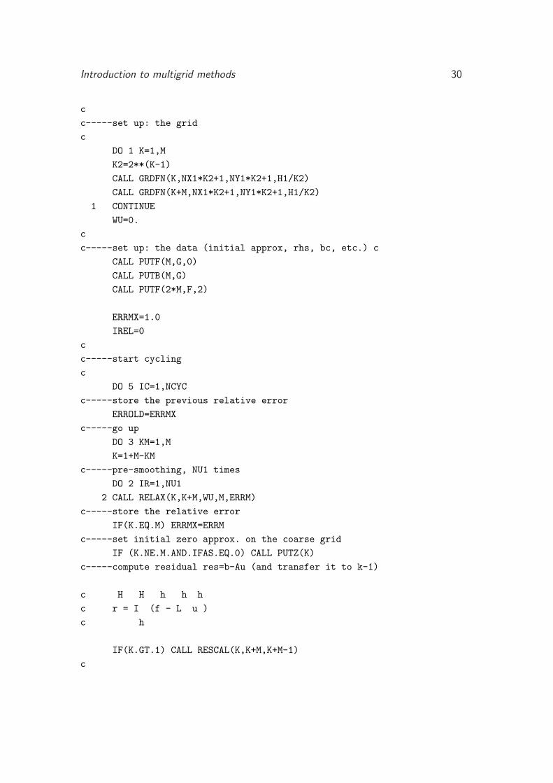
Introduction to multigrid methods 30
c
c-----set up: the grid
c
DO 1 K=1,M
K2=2**(K-1)
CALL GRDFN(K,NX1*K2+1,NY1*K2+1,H1/K2)
CALL GRDFN(K+M,NX1*K2+1,NY1*K2+1,H1/K2)
1 CONTINUE
WU=0.
c
c-----set up: the data (initial approx, rhs, bc, etc.) c
CALL PUTF(M,G,0)
CALL PUTB(M,G)
CALL PUTF(2*M,F,2)
ERRMX=1.0
IREL=0
c
c-----start cycling
c
DO 5 IC=1,NCYC
c-----store the previous relative error
ERROLD=ERRMX
c-----go up
DO 3 KM=1,M
K=1+M-KM
c-----pre-smoothing, NU1 times
DO 2 IR=1,NU1
2 CALL RELAX(K,K+M,WU,M,ERRM)
c-----store the relative error
IF(K.EQ.M) ERRMX=ERRM
c-----set initial zero approx. on the coarse grid
IF (K.NE.M.AND.IFAS.EQ.0) CALL PUTZ(K)
c-----compute residual res=b-Au (and transfer it to k-1)
c H H h h h
c r = I (f - L u )
c h
IF(K.GT.1) CALL RESCAL(K,K+M,K+M-1)
c

Introduction to multigrid methods 31
c-----set initial approx. on the coarse grid
IF (K.NE.1.AND.IFAS.EQ.1) CALL PUTU(K,K-1)
c-----compute the right-hand side
c H H h h h H H h
c f = I (f - L u ) + L (I u)
c h h
IF(K.GT.1.AND.IFAS.EQ.1) CALL CRSRES(K-1,K+M-1)
3 CONTINUE
c
c-----go down
DO 5 K=1,M
DO 4 IR=1,NU2
4 CALL RELAX(K,K+M,WU,M,ERRM)
c-----interpolate the coarse solution (error function)
c to the next finer grid and add to the existing approximation
c
c h h h H H h
c u = u + I (u - I u )
c
IF(IFAS.EQ.1.AND.K.LT.M) CALL SUBTRT(K+1,K)
c
IF(K.LT.M) CALL INTADD(K,K+1)
c
c-----compute the convergence factor using the relative c error
IF(K.EQ.M) write(*,*) ’rho ’, errmx/errold
5 CONTINUE
C
C PRINT THE SOLUTION (FINEST GRID) C
999 CONTINUE
OPEN(UNIT=17,FILE=’TEST.DAT’,STATUS=’UNKNOWN’)
CALL KEY(M,IST,II,JJ,H)
JSTEP=17
IF(JJ.GT.9) JSTEP=INT(JJ/9.)+1
DO 90 I=1,II
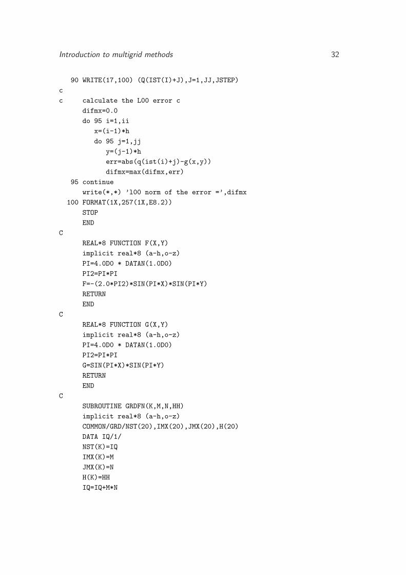
Introduction to multigrid methods 32
90 WRITE(17,100) (Q(IST(I)+J),J=1,JJ,JSTEP)
c
c calculate the L00 error c
difmx=0.0
do 95 i=1,ii
x=(i-1)*h
do 95 j=1,jj
y=(j-1)*h
err=abs(q(ist(i)+j)-g(x,y))
difmx=max(difmx,err)
95 continue
write(*,*) ’l00 norm of the error =’,difmx
100 FORMAT(1X,257(1X,E8.2))
STOP
END
C
REAL*8 FUNCTION F(X,Y)
implicit real*8 (a-h,o-z)
PI=4.0D0 * DATAN(1.0D0)
PI2=PI*PI
F=-(2.0*PI2)*SIN(PI*X)*SIN(PI*Y)
RETURN
END
C
REAL*8 FUNCTION G(X,Y)
implicit real*8 (a-h,o-z)
PI=4.0D0 * DATAN(1.0D0)
PI2=PI*PI
G=SIN(PI*X)*SIN(PI*Y)
RETURN
END
C
SUBROUTINE GRDFN(K,M,N,HH)
implicit real*8 (a-h,o-z)
COMMON/GRD/NST(20),IMX(20),JMX(20),H(20)
DATA IQ/1/
NST(K)=IQ
IMX(K)=M
JMX(K)=N
H(K)=HH
IQ=IQ+M*N
Introduction to multigrid methods 33
RETURN
END
C
SUBROUTINE KEY(K,IST,M,N,HH)
implicit real*8 (a-h,o-z)
COMMON/GRD/NST(20),IMX(20),JMX(20),H(20)
DIMENSION IST(200)
M=IMX(K)
N=JMX(K)
IS=NST(K)-N-1
DO 1 I=1,M
IS=IS + N
1 IST(I)=IS
HH=H(K)
RETURN
END
C
SUBROUTINE PUTF(K,F,NH)
implicit real*8 (a-h,o-z)
COMMON Q(18000)
DIMENSION IST(200)
CALL KEY (K,IST,II,JJ,H)
H2=H**NH
DO 1 I=1,II
DO 1 J=1,JJ
X=(I-1)*H
Y=(J-1)*H
1 Q(IST(I)+J)=F(X,Y)*H2
RETURN
END
C
SUBROUTINE PUTZ(K)
implicit real*8 (a-h,o-z)
COMMON Q(18000)
DIMENSION IST(200)
CALL KEY(K,IST,II,JJ,H)
DO 1 I=1,II
DO 1 J=1,JJ
1 Q(IST(I)+J)=0.
RETURN
END

Introduction to multigrid methods 34
C
SUBROUTINE PUTU(KF,KC)
implicit real*8 (a-h,o-z)
COMMON Q(18000)
DIMENSION IUF(200), IUC(200)
CALL KEY(KF,IUF,IIF,JJF,HF)
CALL KEY(KC,IUC,IIC,JJC,HC)
DO 1 IC=1,IIC
IF=2*IC-1
IFO=IUF(IF)
ICO=IUC(IC)
JF=-1
DO 1 JC=1,JJC
JF=JF+2
Q(ICO+JC)=Q(IFO+JF)
1 CONTINUE
RETURN
END
C
SUBROUTINE PUTB(K,F)
implicit real*8 (a-h,o-z)
COMMON Q(18000)
DIMENSION IST(200)
CALL KEY (K,IST,II,JJ,H)
DO 1 I=1,II
X=(I-1)*H
Y=0.0
Q(IST(I)+1)=F(X,Y)
Y=(JJ-1)*H
Q(IST(I)+JJ)=F(X,Y)
1 CONTINUE
DO 2 J=1,JJ
Y=(J-1)*H
X=0.0
Q(IST(1)+J)=F(X,Y)
X=(II-1)*H
Q(IST(II)+J)=F(X,Y)
2 CONTINUE
RETURN
END
C
Introduction to multigrid methods 35
SUBROUTINE SUBTRT(KF,KC)
implicit real*8 (a-h,o-z)
COMMON Q(18000)
DIMENSION IUF(200),IUC(200)
CALL KEY(KF,IUF,IIF,JJF,HF)
CALL KEY(KC,IUC,IIC,JJC,HC)
DO 1 IC=1,IIC
IF=2*IC-1
IFO=IUF(IF)
ICO=IUC(IC)
JF=-1
DO 1 JC=1,JJC
JF=JF+2
Q(ICO+JC)=Q(ICO+JC)-Q(IFO+JF)
1 CONTINUE
RETURN
END
C
SUBROUTINE INTADD(KC,KF)
implicit real*8 (a-h,o-z)
COMMON Q(18000)
DIMENSION ISTC(200),ISTF(200)
CALL KEY(KC,ISTC,IIC,JJC,HC)
CALL KEY(KF,ISTF,IIF,JJF,HF)
HF2=HF*HF
DO 1 IC=2,IIC
IF=2*IC-1
JF=1
IFO=ISTF(IF)
IFM=ISTF(IF-1)
ICO=ISTC(IC)
ICM=ISTC(IC-1)
DO 1 JC=2,JJC
JF=JF+2
A=.5*(Q(ICO+JC)+Q(ICO+JC-1))
AM=.5*(Q(ICM+JC)+Q(ICM+JC-1))
Q(IFO+JF) = Q(IFO+JF)+Q(ICO+JC)
Q(IFM+JF) = Q(IFM+JF)+.5*(Q(ICO+JC)+Q(ICM+JC))
Q(IFO+JF-1)=Q(IFO+JF-1)+A
1 Q(IFM+JF-1)=Q(IFM+JF-1)+.5*(A+AM)
RETURN

Introduction to multigrid methods 36
END
C
SUBROUTINE RESCAL(KF,KRF,KRC)
implicit real*8 (a-h,o-z)
COMMON Q(18000)
DIMENSION IUF(200),IRF(200),IRC(200)
CALL KEY(KF,IUF,IIF,JJF,HF)
CALL KEY(KRF,IRF,IIF,JJF,HF)
CALL KEY(KRC,IRC,IIC,JJC,HC)
IIC1=IIC-1
JJC1=JJC-1
HF2=HF*HF
DO 1 IC=2,IIC1
ICR=IRC(IC)
IF=2*IC-1
JF=1
IFR=IRF(IF)
IF0=IUF(IF)
IFM=IUF(IF-1)
IFP=IUF(IF+1)
DO 1 JC=2,JJC1
JF=JF+2
S=Q(IF0+JF+1)+Q(IF0+JF-1)+Q(IFM+JF)+Q(IFP+JF)
1 Q(ICR+JC)=4.*(Q(IFR+JF)-S+4.*Q(IF0+JF))
RETURN
END
C
SUBROUTINE CRSRES(K,KRHS)
implicit real*8 (a-h,o-z)
COMMON Q(18000)
DIMENSION IST(200),IRHS(200)
CALL KEY(K,IST,II,JJ,H)
CALL KEY(KRHS,IRHS,II,JJ,H)
I1=II-1
J1=JJ-1
H2=H*H
DO 1 I=2,I1
IR=IRHS(I)
IO=IST(I)
IM=IST(I-1)
IP=IST(I+1)
Introduction to multigrid methods 37
DO 1 J=2,J1
A=-Q(IR+J)-Q(IO+J+1)-Q(IO+J-1)-Q(IM+J)-Q(IP+J)
1 Q(IR+J)=-A-4.*Q(IO+J)
RETURN
END
C
SUBROUTINE RELAX(K,KRHS,WU,M,ERRM)
c-----Gauss-Seidel
implicit real*8 (a-h,o-z)
COMMON Q(18000)
DIMENSION IST(200),IRHS(200)
CALL KEY(K,IST,II,JJ,H)
CALL KEY(KRHS,IRHS,II,JJ,H)
I1=II-1
J1=JJ-1
ERR=0.
ERRQ=0.
ERRM=0.
H2=H*H
COEFF=4.
DO 1 I=2,I1
IR=IRHS(I)
IQ=IST(I)
IM=IST(I-1)
IP=IST(I+1)
DO 1 J=2,J1
A=Q(IR+J)-Q(IQ+J+1)-Q(IQ+J-1)-Q(IM+J)-Q(IP+J)
c-----residual norm L2
ERR=ERR+(A+COEFF*Q(IQ+J))**2
QOLD=Q(IQ+J)
Q(IQ+J)=-A/(COEFF)
ERRQ=ERRQ+(QOLD-Q(IQ+J))**2
c-----relative ’dynamic’ error norm max
Z=abs(QOLD-Q(IQ+J))
ERRM=MAX(ERRM,Z)
1 CONTINUE
ERR=SQRT(ERR)/H
ERRQ=SQRT(ERRQ)
WU=WU+4.**(K-M)
write(*,2) K,ERRQ,WU
Introduction to multigrid methods 38
2 FORMAT(’ LEVEL’,I2,’ RESIDUAL NORM=’,E10.3,’ WORK=’,F7.3)
RETURN
END
C
References
[1] N.S. Bakhvalov, On the convergence of a relaxation method with
natural constraints on the elliptic operator. USSR Computational
Math. and Math. Phys. 6 (1966) 101.
[2] D.S. Balsara and A. Brandt, Multilevel Methods for Fast Solution
of N -Body and Hybrid Systems. In: Hackbusch-Trottenberg [25].
[3] A. Brandt, Multi-Level Adaptive Technique (MLAT) for Fast Nu-
merical Solution to Boundary-Value Problems. In: H. Cabannes
and R. Temam (eds.), Proceedings of the Third International Con-
ference on Numerical Methods in Fluid Mechanics, Paris 1972.
Lecture Notes in Physics 18, Springer-Verlag, Berlin, 1973.
[4] A. Brandt, Multi-Level Adaptive Solutions to Boundary-Value
Problems. Math. Comp. 31 (1977) 333-390.
[5] A. Brandt and N. Dinar, Multigrid Solutions to Elliptic Flow Prob-
lems. In: S.V. Parter (ed.), Numerical Methods for Partial Differ-
ential Equations, Academic Press, New York, 1979.
[6] A. Brandt, S. McCormick and J. Ruge, Multigrid Methods for
Differential Eigenproblems. SIAM J. Sci. Stat. Comput. 4 (1983)
244-260.
[7] A. Brandt, Multi-grid techniques: 1984 guide with applications
to fluid dynamics. GMD-Studien. no 85, St. Augustin, Germany,
1984.

Introduction to multigrid methods 39
[8] A. Brandt, Rigorous Local Mode Analysis of Multigrid. Lecture
at the 2nd European Conference on Multigrid Methods, Cologne,
Oct. 1985. Research Report, The Weizmann Institute of Science,
Israel, Dec. 1987.
[9] A. Brandt and A.A. Lubrecht, Multilevel Matrix Multiplication and
Fast Solution of Integral Equations. J. Comp. Phys. 90 (1990)
348-370.
[10] A. Brandt and J. Greenwald, Parabolic Multigrid Revisited. In:
Hackbusch-Trottenberg [25].
[11] A. Brandt, Multilevel computations of integral transforms and par-
ticle interactions with oscillatory kernels. Comp. Phys. Commun.
65 (1991) 24-38.
[12] A. Brandt, D. Ron and D.J. Amit, Multi-Level Approaches
to Discrete-State and Stochastic Problems. In: Hackbusch-
Trottenberg [24].
[13] A. Brandt and D. Sidilkover , Multigrid solution to steady-state
two-dimensional conservation laws, SIAM Journal on Numerical
Analysis, 30 (1993), p.249-274.
[14] A. Brandt, Multigrid Methods in Lattice Field Computations. Nucl.
Phys. (Proc.Suppl.) B21 (1992) 1-45.
[15] R.P. Fedorenko, A relaxation method for solving elliptic difference
equations. USSR Computational Math. and Math. Phys. 1 (1962)
1092.
[16] R.P. Fedorenko, The rate of convergence of an iterative process.
USSR Computational Math. and Math. Phys. 4 (1964) 227.
[17] J. Goodman and A.D. Sokal, Multigrid Monte Carlo for lattice
field theories. Phys. Rev. Lett. 56 (1986) 1015.

Introduction to multigrid methods 40
[18] W. Hackbusch, A multi-grid method applied to a boundary prob-
lem with variable coefficients in a rectangle. Report 77-17, Institut
fur Angewandte Mathematik, Universitat Koln, 1977.
[19] W. Hackbusch, On the computation of approximate eigenvalues
and eigenfunctions of elliptic operators by means of a multi-grid
method. SIAM J. Numer. Anal. 16 (1979) 201-215.
[20] W. Hackbusch, Parabolic Multi-Grid Methods. In: R. Glowinski
and J.L. Lions (eds.), Computing Methods in Applied Sciences
and Engineering, VI. Proc. of the sixth international symposium,
Versailles, Dec.1983, North-Holland, Amsterdam, 1984.
[21] W. Hackbusch, Multi-Grid Methods and Applications. Springer-
Verlag, Heidelberg, 1985.
[22] W. Hackbusch, Multi-Grid Methods of the Second Kind. In: D.J.
Paddon and H. Holstein (eds.), Multigrid Methods for Integral and
Differential Equations. Claredon Press, Oxford, 1985.
[23] W. Hackbusch and U. Trottenberg (eds.), Multi-Grid Methods,
Proceedings, Koln-Porz, Nov. 1981, Lecture Notes in Mathematics
960, Springer-Verlag, Berlin, 1982.
[24] W. Hackbusch and U. Trottenberg (eds.), Multigrid Methods II, II.
Proc. of the European Conference on Multigrid Methods, Cologne,
Oct. 1985, Lecture Notes in Mathematics 1228, Springer-Verlag,
Berlin, 1986.
[25] W. Hackbusch and U. Trottenberg (eds.), Multigrid Methods III,
III. Proc. of the European Conference on Multigrid Methods, Bonn,
Oct. 1990, Birkhauser, Berlin, 1991.
[26] P.W. Hemker and H. Schippers, Multiple grid methods for the
solution of Fredholm integral equations of the second kind. Math.
Comp. 36 (1981) 215-232.

Introduction to multigrid methods 41
[27] P.W. Hemker and P. Wesseling (eds.), Multigrid Methods IV, Pro-
ceedings of the IV European Multigrid Conference, Amsterdam,
Jul. 1993, International Series on Numerical Mathematics, Vol.
116, Birkhauser Verlag, Basel, 1994.
[28] Van Emden Henson, Multigrid for Nonlinear Problems: an
Overview, presented by Van Emden Henson at the SPIE 15th An-
nual Symposium on Electronic Imaging, Santa Clara, California,
January 23, 2003.
[29] T. Kalkreuter, Multigrid Methods for the Computation of Propa-
gators in Gauge Fields. DESY 92-158.
[30] L. Lapidus and G.E. Pinder, Numerical Solution of Partial Differ-
ential Equations in Science and Engineering. John Wiley & Sons,
New York, 1982.
[31] G. Mack and S. Meyer, The effective action from multigrid Monte
Carlo. Nucl. Phys. (Proc. Suppl.) 17 (1990) 293.
[32] J. Mandel et al., Copper Mountain Conference on Multigrid Meth-
ods. IV. Proc. of the Copper Mountain Conference on Multi-
grid Methods, Copper Mountain, April 1989, SIAM, Philadelphia,
1989.
[33] H.D. Mittelmann and H. Weber, Multi-Grid Methods for Bifurca-
tion Problems. SIAM J. Sci. Stat. Comput. 6 (1985) 49.
[34] W.A. Mulder, A new multigrid approach to convection problems,
Journal of Computational Physics, v.83 n.2, p.303-323, Aug. 1989
[35] K. Stuben, Algebraic Multigrid (AMG): An Introduction with Ap-
plications, GMD Report 53, March 1999.
[36] K. Stuben and U. Trottenberg, Multigrid Methods: Fundamen-
tal Algorithms, Model Problem Analysis and Applications. In:
Hackbusch-Trottenberg [23].

Introduction to multigrid methods 42
[37] S. Ta’asan, Multigrid Methods for Locating Singularities in Bifur-
cation Problems. SIAM J. Sci. Stat. Comput. 11 (1990) 51-62.
[38] S. Ta’asan, Introduction to shape design and control; Theoretical
tools for problem setup; Infinite dimensional preconditioners for
optimal design. In: Inverse Design and Optimisation Methods, VKI
LS 1997-05.
[39] C.-A. Thole and U. Trottenberg, Basic smoothing procedures
for the multigrid treatment of elliptic 3D-operators. Appl. Math.
Comp. 19 (1986) 333-345.
[40] U. Trottenberg, C. Oosterlee, and A. Schuller, Multigrid, Aca-
demic Press, London, 2001.
[41] S. Vandewalle and R. Piessens, Efficient Parallel Algorithms for
Solving Initial-Boundary Value and Time-Periodic Parabolic Par-
tial Differential Equations. SIAM J. Sci. Stat. Comput. 13 (1992)
1330-1346.
[42] P. Wesseling, A survey of Fourier smoothing analysis results. In:
Hackbusch-Trottenberg [25].