an introduction to algebraic multigrid (amg) algorithms -
TRANSCRIPT
An Introduction to Algebraic Multigrid(AMG) Algorithms
Derrick Cerwinsky and Craig C. Douglas
1/84

Introduction
Almost all numerical methods for solving PDEs will at some point bereduced to solving
A~x = ~b. (1)
Many methods exist for solving this equation. Most discretizationmethods will impose some structure on A which can be exploited.In this talk we will examine a collection of methods which can efficientlysolve this problem, as well as a software package that can helpdetermine the best method to use.
2/84
Multigrid Methods
Multigrid methods are accelerators for iterative solvers.Given a computational grid, an approximation to the solution isfound.The problem is then restricted to a sub-grid, called the coarse grid.On the coarse grid the residual problem is solved.The solution to the residual problem is then interpolated back tothe full mesh (called the fine grid) where the correction is made tothe approximation of the solution.Multigrid methods are very effective. However, they require adetailed knowledge of the underlying computational mesh.
3/84
Algebraic Multigrid (AMG) Methods
Algebraic Multigrid Methods differ from multigrid method only in themethod of coarsening.While multigrid methods require knowledge of the mesh, AMG methodsextract all the needed information from the system matrix.It is in this coarsening step that most AMG methods differ.
4/84

AMGLab
5/84

AMGLab
AMGLab is a software package which runs in MATLAB.The goals for AMGLab:
AMGLab is designed to be an easy to use tool with a gentlelearning curve.AMGLab has a large collection of methods which are easilyaccessed and compared.AMGLab can run custom problems with minimal setup time.AMGLab is powerful enough to run moderately sized problems.
Most of the complexity in an AMG method is in the coarsening phase.
6/84

Ruge–Stüben
7/84
Ruge–Stüben
The Ruge–Stüben method was introduced around 1981.The method works in two passes.
The first pass will make a selection of coarse nodes based on thenumber of strong connections that each node has.The second pass is a refinement pass. It checks to make sure thereare enough coarse nodes that information is not lost.
8/84
Ruge–Stüben
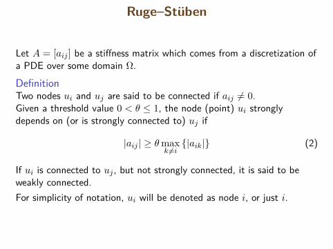
Let A = [aij ] be a stiffness matrix which comes from a discretization ofa PDE over some domain Ω.
DefinitionTwo nodes ui and uj are said to be connected if aij 6= 0.Given a threshold value 0 < θ ≤ 1, the node (point) ui stronglydepends on (or is strongly connected to) uj if
|aij | ≥ θmaxk 6=i|aik| (2)
If ui is connected to uj , but not strongly connected, it is said to beweakly connected.For simplicity of notation, ui will be denoted as node i, or just i.
9/84

Ruge–Stüben
DefinitionThe set of grid points selected to be part of the coarse grid will becalled C. An element in C will be called a C-point. The set of pointsnot selected to be in C will be called fine points and will belong to theset F . Points in F will be called F-points.Note that F and C will partition the grid.
10/84
Ruge–Stüben
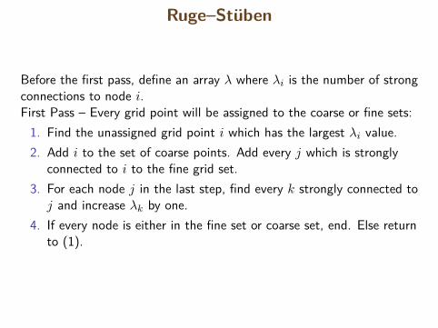
Before the first pass, define an array λ where λi is the number of strongconnections to node i.First Pass – Every grid point will be assigned to the coarse or fine sets:1. Find the unassigned grid point i which has the largest λi value.2. Add i to the set of coarse points. Add every j which is strongly
connected to i to the fine grid set.3. For each node j in the last step, find every k strongly connected toj and increase λk by one.
4. If every node is either in the fine set or coarse set, end. Else returnto (1).
11/84
Ruge–Stüben
The second pass will check for any fine–fine node connections which donot have a common coarse node. If any such fine nodes are found, oneof the fine nodes will be made a coarse node.
12/84

Ruge–Stüben
DefinitionFor each fine-grid point i, define Ni, the neighborhood of i, to be theset of all points j 6= i such that aij 6= 0. These points can be dividedinto three categories:
The neighboring coarse-grid points that strongly influence i; this isthe coarse interpolation set for i, denoted by Ci;The neighboring fine-grid points that strongly influence i, denotedby Ds
i ;The points that do not strongly influence i, denoted by Dw
i ; thisset may contain both coarse- and fine-grid points; it is called theset of weakly connected neighbors.
13/84
Ruge–Stüben
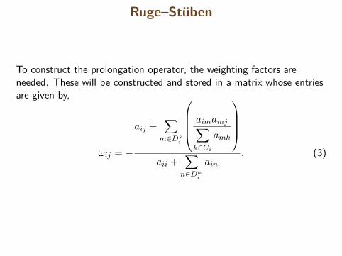
To construct the prolongation operator, the weighting factors areneeded. These will be constructed and stored in a matrix whose entriesare given by,
ωij = −
aij +∑m∈Ds
i
aimamj∑k∈Ci
amk
aii +
∑n∈Dw
i
ain. (3)
14/84
Ruge–Stüben
The prolongation operator is constructed row wise. If i is a coarse node,then the ith row will be the identity. If i is a fine node, then thecorresponding row of the matrix of weights is used.
15/84

Beck Algorithm
16/84

Beck
The Beck algorithm was introduced in 1999 by Rudolf Beck. Thealgorithm is a simple coarsening strategy related to to the Ruge–Stübenmethod.This method is very simple to implement, and works on many of thesame problems as more complex methods, and with similar results.The idea is to look at the graph of the stiffness matrix rather then at thestrength of the connections. That is, all connections are treated equally.
17/84

Beck
The algorithm is as follows.1. Choose the smallest node i which is not in the coarse or fine set,
and add it to the coarse set.2. Add all nodes connected to node i from the last step to the fine set.3. Repeat steps 1 and 2 until all nodes are in the coarse or fine set.
18/84
Beck
For each node k in the fine set, define λk to be the number of coarsepoints connected to k.The prolongation operator is constructed row wise, like in Ruge–Stüben.
Pij =λi−1, if j ∈ C and i is connected to j0, otherwise (4)
19/84
Smoothed Aggregation
20/84

Smoothed Aggregation
DefinitionLet A be a stiffness matrix from a discretization of some PDE on adomain Ω.Define the strongly–coupled neighborhood of node i for a fixedε ∈ [0, 1) as
Ni(ε) =j : |aij ≥ ε
√aiiajj
(5)
21/84

Smoothed Aggregation
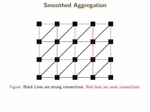
The method will work in two main passes.First, aggregates will be chosen based on neighborhoods of strongconnections. Only full neighborhoods will be selected.
22/84
Smoothed Aggregation
Figure: Black Lines are strong connections. Red lines are weak connections.
23/84
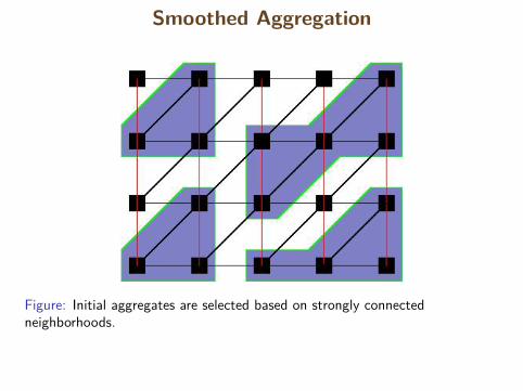
Smoothed Aggregation
Figure: Initial aggregates are selected based on strongly connectedneighborhoods.
24/84
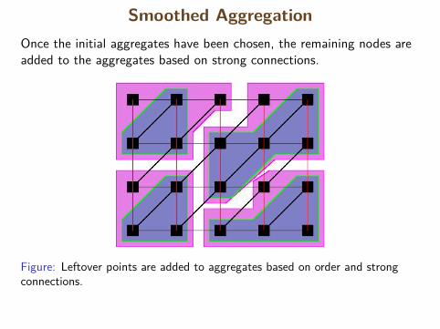
Smoothed AggregationOnce the initial aggregates have been chosen, the remaining nodes areadded to the aggregates based on strong connections.
Figure: Leftover points are added to aggregates based on order and strongconnections.
25/84

Smoothed Aggregation
Once the aggregates are chosen, the prolongation matrix must beformed. This is done by making an initial guess for the operator, andrefining it with a smoothing step.Define Ci as the set of nodes in aggregate i, and
Pi,j =
1 if i ∈ Cj0 otherwise . (6)
26/84
Smoothed Aggregation
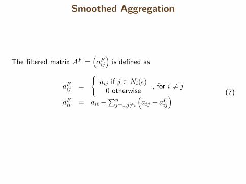
The filtered matrix AF =(aFij
)is defined as
aFij =aij if j ∈ Ni(ε)
0 otherwise , for i 6= j
aFii = aii −∑nj=1,j 6=i
(aij − aFij
) (7)
27/84
Smoothed Aggregation
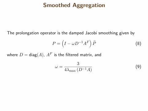
The prolongation operator is the damped Jacobi smoothing given by
P =(I − ωD−1AF
)P (8)
where D = diag(A), AF is the filtered matrix, and
ω = 34λmax (D−1A) (9)
28/84

Implementing Simple AMG Algorithms
29/84

Implementation: Ruge–StübenGiven a threshold value 0 < θ ≤ 1, the variable (point) ui stronglydepends on (or is strongly connected to) the variable (point) uj if
|aij | ≥ θmaxk 6=i|aik| .
Define the set N to be the absolute maximal off diagonal element ineach row of A. Since this is an ordered set, it will be treated as anarray. The entries of N are defined as
Ni = maxj 6=i|aij | .
The matrix of strong connections S is a matrix whose elements aregiven by
Sij =
1, if ui is strongly connected to uj0, otherwise.
Define λ as an array which counts the number of strong connections foreach node,
λi =∑j
Sij .30/84
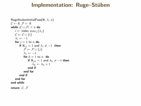
Implementation: Ruge–Stüben
RugeStubenInitialPass(S, λ, n)C ← ∅, F ← ∅while |C ∪ F| < n doi← index maxjλjC ← C ∪ iλi ← −1for j = 1 to n do
if Sij = 1 and λi 6= −1 thenF ← F ∪ jλj ← −1for k = 1 to n do
if Sjk = 1 and λk 6= −1 thenλk ← λk + 1
end ifend for
end ifend for
end whilereturn C, F
31/84
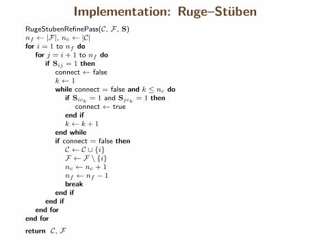
Implementation: Ruge–StübenRugeStubenRefinePass(C, F , S)nf ← |F|, nc ← |C|for i = 1 to nf do
for j = i+ 1 to nf doif Sij = 1 then
connect ← falsek ← 1while connect = false and k ≤ nc do
if Sick= 1 and Sjck
= 1 thenconnect ← true
end ifk ← k + 1
end whileif connect = false thenC ← C ∪ iF ← F \ inc ← nc + 1nf ← nf − 1break
end ifend if
end forend forreturn C, F 32/84
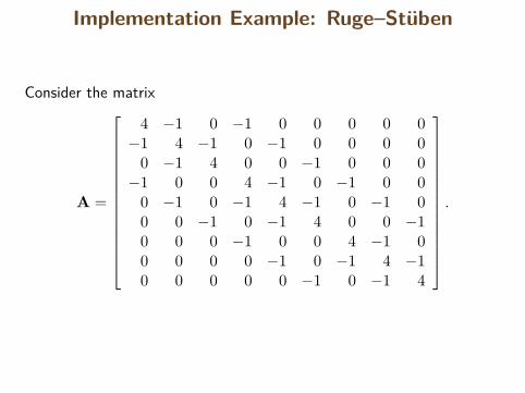
Implementation Example: Ruge–Stüben
Consider the matrix
A =
4 −1 0 −1 0 0 0 0 0−1 4 −1 0 −1 0 0 0 0
0 −1 4 0 0 −1 0 0 0−1 0 0 4 −1 0 −1 0 0
0 −1 0 −1 4 −1 0 −1 00 0 −1 0 −1 4 0 0 −10 0 0 −1 0 0 4 −1 00 0 0 0 −1 0 −1 4 −10 0 0 0 0 −1 0 −1 4
.
33/84
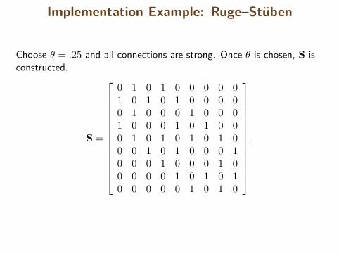
Implementation Example: Ruge–Stüben
Choose θ = .25 and all connections are strong. Once θ is chosen, S isconstructed.
S =
0 1 0 1 0 0 0 0 01 0 1 0 1 0 0 0 00 1 0 0 0 1 0 0 01 0 0 0 1 0 1 0 00 1 0 1 0 1 0 1 00 0 1 0 1 0 0 0 10 0 0 1 0 0 0 1 00 0 0 0 1 0 1 0 10 0 0 0 0 1 0 1 0
.
34/84
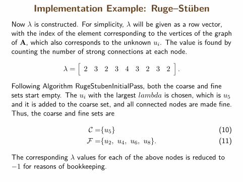
Implementation Example: Ruge–StübenNow λ is constructed. For simplicity, λ will be given as a row vector,with the index of the element corresponding to the vertices of the graphof A, which also corresponds to the unknown ui. The value is found bycounting the number of strong connections at each node.
λ =[
2 3 2 3 4 3 2 3 2].
Following Algorithm RugeStubenInitialPass, both the coarse and finesets start empty. The ui with the largest lambda is chosen, which is u5and it is added to the coarse set, and all connected nodes are made fine.Thus, the coarse and fine sets are
C =u5 (10)F =u2, u4, u6, u8. (11)
The corresponding λ values for each of the above nodes is reduced to−1 for reasons of bookkeeping.
35/84

Implementation Example: Ruge–Stüben
Now, for each of the new fine nodes, each unassigned node has its λvalue increased by 1. Note that if a node is connected to more then onefine node, it is incremented for each fine node it is connected to. So thenew lambda values are
λ =[
4 −1 4 −1 −1 −1 4 −1 4].
All that remains now are the corner nodes, which are all disjoint fromeach other. So, all of the remaining nodes will be made into coarsenodes. The coarse and fine nodes after the first pass are given by,
C =u1, u3, u5, u7, u9 (12)F =u2, u4, u6, u8. (13)
A quick inspection shows that there are no fine–fine connections, so thesecond pass is not needed, and the coarse set is finalized...
36/84

Implementation Example: Ruge–Stüben
This illustrates the process required for the first pass of coarsening. Thecoarse set is in red and the fine set is in blue. Note that the third frameis the compilation of the final four iterations.
Initial Grid First Iteration Final Coarsening
37/84
Implementation Example: Ruge–Stüben
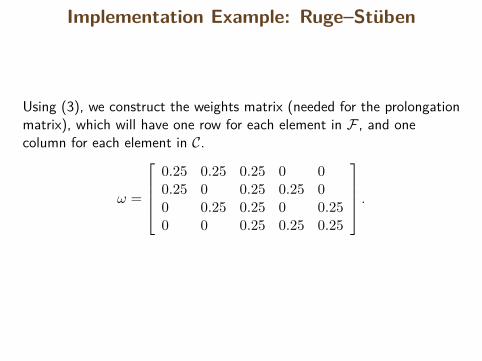
Using (3), we construct the weights matrix (needed for the prolongationmatrix), which will have one row for each element in F , and onecolumn for each element in C.
ω =
0.25 0.25 0.25 0 00.25 0 0.25 0.25 00 0.25 0.25 0 0.250 0 0.25 0.25 0.25
.
38/84

Implementation Example: Ruge–Stüben
The prolongation operator is constructed using the values from ω. Theodd numbered rows correspond to the coarse nodes, so each of theserows is the identity. The even numbered rows come from ω.
P =
1 0 0 0 00.25 0.25 0.25 0 00 1 0 0 00.25 0 0.25 0.25 00 0 1 0 00 0.25 0.25 0 0.250 0 0 1 00 0 0.25 0.25 0.250 0 0 0 1
,
39/84

Implementation Example: Ruge–Stüben
The coarse matrix is Ac = PTAP, or
Ac =
3.5 −0.25 −0.5 −0.25 0
−0.25 3.5 −0.5 0 −0.25−0.5 −0.5 3.0 −0.5 −0.5−0.25 0 −0.5 3.5 −0.25
0 −0.25 −0.5 −0.25 3.5
.
40/84
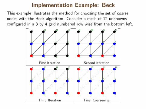
Implementation Example: BeckThis example illustrates the method for choosing the set of coarsenodes with the Beck algorithm. Consider a mesh of 12 unknownsconfigured in a 3 by 4 grid numbered row wise from the bottom left.
First Iteration Second Iteration
Third Iteration Final Coarsening41/84

Implementation Example: Beck
Now consider another example: start with the symmetric positivedefinite matrix
Af =
2 −1 0 0−1 2 −1 0
0 −1 2 −10 0 −1 2
.Using Beck’s algorithm, the coarse and fine sets are defined as
C = u1, u3 and F = u2, u4 .
42/84

Implementation Example: Beck
For each element of F , σi must be computed. Since u2 is connected toboth u1 and u3, σ2 = 2. However, u4 is only connected to u3, soσ4 = 1. Hence,
P =
1 012
12
0 10 1
. (14)
Note that while the 3rd and 4th rows are the same, it is for differentreasons. The 3rd row is [0 1] because u3 ∈ C and it is the secondelement on the coarse grid. The 4th row is [0 1] because u4 ∈ F buthas only one connection to a coarse point. Finally,
Ac = PTAfP =[
1.5 −0.5−0.5 1.5
], (15)
43/84
Matlab Tricks
Implementing AMG in Matlab is relatively easy assuming that youfollow some simple programming rules:
Store all matrices as sparse matrices.Use data structures that are indexed by the level = 1, 2, · · ·Use a lot of small, carefully written functions that are each efficient.Be very careful with matrix arithmetic since Matlab likes to storetemprary matrices as dense matrices.Matlab allows variables to be declared global. In some cases thisbecomes almost essential when implementing AMG.If you have a set of global constants, put them all in a functionthat all other functions call first.Use recursion carefully, but use it.
44/84
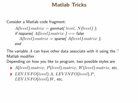
Matlab Tricks
Consider a Matlab code fragment:A(level).matrix = genmat( level, N(level) );if issparse( A(level).matrix ) == falseA(level).matrix = sparse( A(level).matrix );
end
The variable A can have other data associate with it using the ’.’Matlab modifier.Depending on how you like to program, two possible styles are
A(level).matrix, P (level).matrix, W (level).matrix, etc.LEV INFO(level).A, LEV INFO(level).P ,LEV INFO(level).W , etc.
45/84
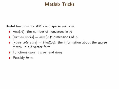
Matlab Tricks
Useful functions for AMG and sparse matrices:nnz(A): the number of nonzeroes in A[nrows,ncols] = size(A): dimensions of A[rows,cols,vals] = find(A): the information about the sparsematrix in a 3-vector formFunctions ones, zeros, and diagPossibly kron
46/84

AMGe
47/84
AMGe
AMGe methods apply to finite element methods for PDEs.AMGe methods use information about the elements for coarsening.The global stiffness matrix is often ill–conditioned for normal AMGmethods. This AMGe method is a pre–conditioner for the stiffnessmatrix.
Define K to be a stiffness matrix from some FEM for a PDE on somedomain Ω, and K(i) as the element (local) stiffness matrix on theelement δ(i).To simplify notation, δ(i) will be denoted simply as element i unlessconfusion will arise.
48/84
AMGe
The idea of this AMGe method is to precondition the element stiffnessmatrices before assembly so that the matrix K will be conditioned forstandard AMG methods.That is to say, replace K(i) with a spectrally equivalent matrix B(i).
DefinitionThe SPSD matrices B ∈ Rn×n and A ∈ Rn×n are called spectrallyequivalent if
∃c1, c2 ∈ R+ : c1 · 〈Bu, u〉 ≤ 〈Au, u〉 ≤ c2 · 〈Bu, u〉 ∀u ∈ Rn (16)
which is briefly denoted by c1 ·B ≤ A ≤ c2 ·B.
49/84
AMGe
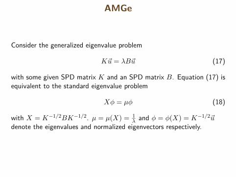
Consider the generalized eigenvalue problem
K~u = λB~u (17)
with some given SPD matrix K and an SPD matrix B. Equation (17) isequivalent to the standard eigenvalue problem
Xφ = µφ (18)
with X = K−1/2BK−1/2. µ = µ(X) = 1λ and φ = φ(X) = K−1/2~u
denote the eigenvalues and normalized eigenvectors respectively.
50/84
AMGe
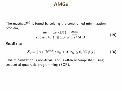
The matrix B(i) is found by solving the constrained minimizationproblem,
minimize κ(X) = µmaxµmin
subject to B ∈ Znr and B SPD . (19)
Recall that
Zn =A ∈ Rn×n : aii > 0, aij ≤ 0, ∀i 6= j
(20)
This minimization is non-trivial and is often accomplished usingsequential quadratic programming (SQP).
51/84
AMGe
The element matrices B(i) are then used to assemble the global stiffnessmatrix A. Standard AMG methods can then be applied to A normally.
While the minimization procedure for each element matrix is expensive,the element matrices are very small in relation to the global stiffnessmatrix. In most problems, the element matrices are similar, and can begrouped into spectrally equivalent classes to reduces the number ofminimizations required.
52/84

Optimization
Assuming that a minimum can be found, a way to test if a point isreally the minimum is required. The Karush, Kuhn and Tuckerconditions (commonly called the KKT conditions) give necessary andsufficient conditions for a point to be a constrained minimum. Theconditions were found independently by Karush (1939) and Kuhn andTucker (1951).
53/84
KKT Conditions
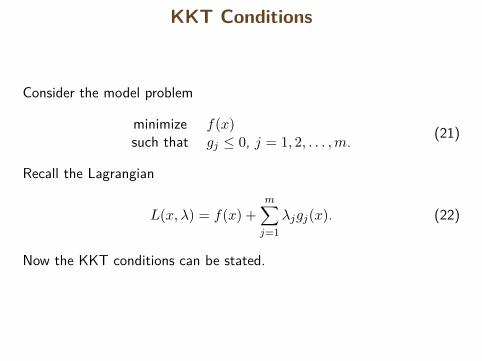
Consider the model problem
minimize f(x)such that gj ≤ 0, j = 1, 2, . . . ,m. (21)
Recall the Lagrangian
L(x, λ) = f(x) +m∑j=1
λjgj(x). (22)
Now the KKT conditions can be stated.
54/84
KKT Conditions
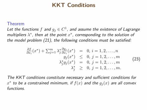
TheoremLet the functions f and gj ∈ C1, and assume the existence of Lagrangemultipliers λ∗, then at the point x∗, corresponding to the solution ofthe model problem (21), the following conditions must be satisfied:
∂f∂xi
(x∗) +∑mj=1 λ
∗j∂gj
∂xi(x∗) = 0, i = 1, 2, . . . , n
gj(x∗) ≤ 0, j = 1, 2, . . . ,mλ∗jgj(x∗) = 0, j = 1, 2, . . . ,m
λ∗j ≥ 0, j = 1, 2, . . . ,m.
(23)
The KKT conditions constitute necessary and sufficient conditions forx∗ to be a constrained minimum, if f(x) and the gj(x) are all convexfunctions.
55/84
Quadratic Programming (QP)
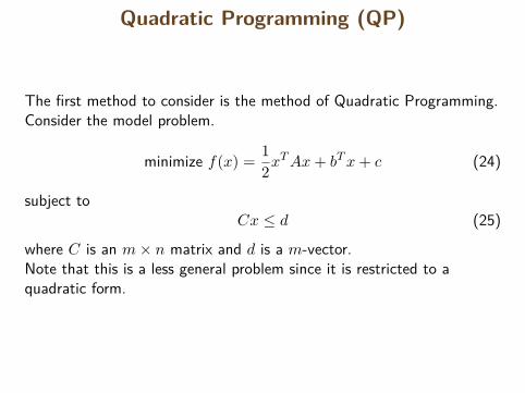
The first method to consider is the method of Quadratic Programming.Consider the model problem.
minimize f(x) = 12x
TAx+ bTx+ c (24)
subject toCx ≤ d (25)
where C is an m× n matrix and d is a m-vector.Note that this is a less general problem since it is restricted to aquadratic form.
56/84
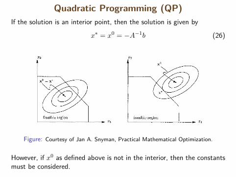
Quadratic Programming (QP)If the solution is an interior point, then the solution is given by
x∗ = x0 = −A−1b (26)
Figure: Courtesy of Jan A. Snyman, Practical Mathematical Optimization.
However, if x0 as defined above is not in the interior, then the constantsmust be considered. 57/84
Quadratic Programming (QP)
A (very) loose definition of an active set of constraints is the constraintsthat are being considered. That is, if the active set if given by g1(x),then the solution must fall on the curve g1. If the active set isg1(x), g2(x) then the solution will be on the intersection of g1 and g2.
58/84
Quadratic Programming (QP)
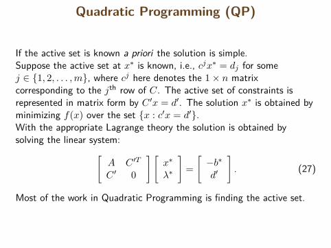
If the active set is known a priori the solution is simple.Suppose the active set at x∗ is known, i.e., cjx∗ = dj for somej ∈ 1, 2, . . . ,m, where cj here denotes the 1× n matrixcorresponding to the jth row of C. The active set of constraints isrepresented in matrix form by C ′x = d′. The solution x∗ is obtained byminimizing f(x) over the set x : c′x = d′.With the appropriate Lagrange theory the solution is obtained bysolving the linear system:[
A C ′T
C ′ 0
] [x∗
λ∗
]=[−b∗d′
]. (27)
Most of the work in Quadratic Programming is finding the active set.
59/84
Quadratic Programming
The method outlined here for identifying the active set is by Theil andVan de Panne (1961). The method simply put says to activate theconstraints one at a time and solve (27). If the solution passes all theconstraints and the KKT condition, then the solution is a minimum. Ifthese conditions are not met, take the active constraints two at a time,testing each solution in turn. Continue adding constraints and testinguntil a solution is found.
60/84

Quadratic Programming (QP)In the following figure, (1), (2), and (3) are constraints. x0 is theunconstrained solution.
Figure: Courtesy of Jan A. Snyman, Practical Mathematical Optimization.
The points a, b, and c are the solutions with the constraints taken oneat a time.The points u, v, and w are the solutions with the constraints two at atime. The optimum solution is v. 61/84
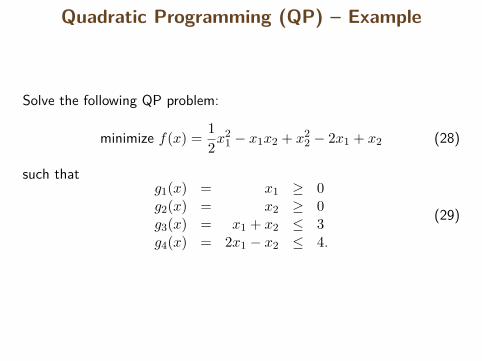
Quadratic Programming (QP) – Example
Solve the following QP problem:
minimize f(x) = 12x
21 − x1x2 + x2
2 − 2x1 + x2 (28)
such thatg1(x) = x1 ≥ 0g2(x) = x2 ≥ 0g3(x) = x1 + x2 ≤ 3g4(x) = 2x1 − x2 ≤ 4.
(29)
62/84
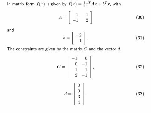
In matrix form f(x) is given by f(x) = 12x
TAx+ bTx, with
A =[
1 −1−1 2
](30)
andb =
[−2
1
]. (31)
The constraints are given by the matrix C and the vector d.
C =
−1 0
0 −11 12 −1
, (32)
d =
0034
. (33)
63/84

The unconstrained solution is x0 = −A−1b = [3, 1]T . However, theconstraints g3 and g4 are not satisfied. The constraints will be activatedone at a time. Taking g1 as active, equation (27) becomes 1 −1 −1
−1 2 0−1 0 0
x1x2λ1
=
2−10
. (34)
Solving this system gives x1x2λ1
=
0−0.5−1.5
. (35)
This violates the KKT condition since λ1 < 0.
64/84
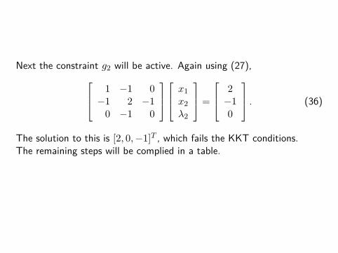
Next the constraint g2 will be active. Again using (27), 1 −1 0−1 2 −1
0 −1 0
x1x2λ2
=
2−10
. (36)
The solution to this is [2, 0,−1]T , which fails the KKT conditions.The remaining steps will be complied in a table.
65/84

Active Set Result0
[3 1
]T fails g3
1[
0 −0.5 −1.5]T fails KKT
2[
2 0 −1]T fails KKT
3[
2.4 0.6 0.2]T fails g4
4[
2.4 0.8 0.2]T fails g3
1, 2[
0 0 −2 1]T fails KKT
1, 3[
0 3 −12 −7]T fails KKT
1, 4[
0 −4 −12 7]T fails KKT
2, 3[
3 0 −3 −1]T fails KKT
2, 4[
2 0 −1 0]T fails KKT
3, 4[
2.3333 0.6667 0.1111 0.1111]T pass
So with the active constraints g3 and g4, a minimum is found atx∗ = [2.3333, 0.6667]T .
66/84
Sequential Quadratic Programming (SQP)
The QP method is very good for optimization, but it is restricted by theform of the problem. So a different method needs to be employed tosolve a general problem.This is the motivation for the Sequential Quadratic Programming(SQP) method.The SQP method is based on the application of Newton’s method todetermine x∗ and λ∗ from the KKT conditions of the constrainedoptimization problem. The determination of the Newton step isequivalent to the solution of a QP problem.
67/84

Sequential Quadratic Programming (SQP)
Consider the problem
minimize f(x)such that gj(x) ≤ 0; j = 1, 2, . . . ,m
hj(x) = 0; j = 1, 2, . . . , r.(37)
Given estimates(xk, λk, µk
), k = 0, 1, . . . , to the solution and
respective Lagrange multiplier values, with λk ≥ 0, then the Newtonstep s of the k + 1 iteration, such that xk+1 = xk + s is given by thesolution to the following k-th QP problem.
68/84

Sequential Quadratic Programming (SQP)QP-k
(xk, λk, µk
): Minimize with respect to s
F (s) = f(xk) +∇T f(xk)s+ 12s
THL(xk)s (38)
such that
g(xk) +[∂g(xk)∂x
]Ts ≤ 0 (39)
and
h(xk) +[∂h(xk)∂x
]Ts = 0 (40)
and where g = [g1, g2, . . . , gm]T , h = [h1, h2, . . . , hr]T and the Hessianof the classical Lagrangian with respect to x is
HL(xk) = ∇2f(xk) +m∑
j=1λk
j∇2gj(xk) +r∑
j=1µk
j∇2hj(xk). (41)
69/84
Sequential Quadratic Programming (SQP)
The solution of QP-k does not only give s, but also the Lagrangemultipliers λk+1 and µk+1 from the solution of equation (27). So withxk+1 = xk + s, the next QP problem can be constructed.This iterative process continues until xk converges to the real minimum.Because this is Newton iteration, the convergence is fast provided thata good initial value was chosen.
70/84
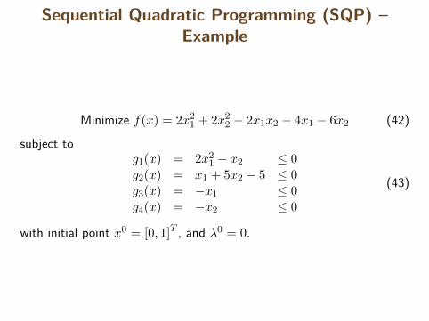
Sequential Quadratic Programming (SQP) –Example
Minimize f(x) = 2x21 + 2x2
2 − 2x1x2 − 4x1 − 6x2 (42)
subject tog1(x) = 2x2
1 − x2 ≤ 0g2(x) = x1 + 5x2 − 5 ≤ 0g3(x) = −x1 ≤ 0g4(x) = −x2 ≤ 0
(43)
with initial point x0 = [0, 1]T , and λ0 = 0.
71/84

The first step is to construct the function F from equation (38). Both∇f(xk) and HL(xk) are needed for the construction. To computeHL(xk) we also need ∇2f(xk), and ∇2gj(xk) for j = 1, . . . , 4.
∇f(xk) =[
4x1 − 2x2 − 44x2 − 2x1 − 6
](44)
∇2f(xk) =[
4 −2−2 4
](45)
∇2g1(xk) =[
4 00 0
](46)
∇2gi(xk) =[
0 00 0
], for i = 2, 3, 4 (47)
72/84
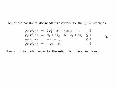
Each of the constants also needs transformed for the QP-k problems.
g1(xk, s) = 2x21 − x2 + 4x1s1 − s2 ≤ 0
g2(xk, s) = x1 + 5x2 − 5 + s1 + 5s2 ≤ 0g3(xk, s) = −x1 − s2 ≤ 0g4(xk, s) = −x2 − s2 ≤ 0
(48)
Now all of the parts needed for the subproblem have been found.
73/84
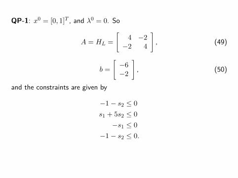
QP-1: x0 = [0, 1]T , and λ0 = 0. So
A = HL =[
4 −2−2 4
], (49)
b =[−6−2
], (50)
and the constraints are given by
−1− s2 ≤ 0s1 + 5s2 ≤ 0−s1 ≤ 0
−1− s2 ≤ 0.
74/84
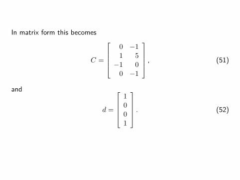
In matrix form this becomes
C =
0 −11 5−1 0
0 −1
, (51)
and
d =
1001
. (52)
75/84

Using the QP method outlined above, the solution is given by s1s2λ2
=
1.129−0.22581.0323
. (53)
x1 = x0 + s =[
1.12900.7742
], (54)
and
λ1 =
0
1.032300
. (55)
Now that x1 and λ1 have been computed, the next QP subproblem canbe constructed and solved.
76/84

The solution is summarized in the following table.
xk sk error[0, 1] [1.129,−0.2258] 0.6720
[1.1290, .07742] [−0.3764, 0.0753] 0.9200[0.7526, 0.8495] [−0.0883, 0.0177] 0.0955[0.6643, 0.8671] [−0.0055, 0.0011] 0.0055[0.6589, 0.8682] 0
(56)
x5 = [0.6589, 0.8682]T which is the minimum to 4 digits.
77/84

Sequential Quadratic Programming (SQP) –Comments
The GoodSQP method converges very fast.The implementation is simple.The method works on very general problems.
The Bad
and the Ugly
The high rate of convergence requires a good initial guess.Computing the Hessian in a complex problem can range fromnon-trivial to impossible.
78/84

Sequential Quadratic Programming (SQP) –Comments
The GoodSQP method converges very fast.The implementation is simple.The method works on very general problems.
The Bad and the UglyThe high rate of convergence requires a good initial guess.Computing the Hessian in a complex problem can range fromnon-trivial to impossible.
78/84
Quasi-Newton Update
The SQP method is a very effective method provide that the derivativesof the function to be optimized are available. In many applications thederivatives of the function being optimized are not easily calculated andmust be approximated. A common method for approximating theHessian is by a quasi-Newton update.
79/84
Quasi-Newton Update
Some new notation is needed.
DefinitionThe Lagrangian of the model problem (21) is given by
L(x, λ) = f(x) + λT g(x), (57)
where x is a KKT point with associated Lagrange multipliers λ.The notation ∇xL(x, λ) refers to the gradient of L with respect to xonly. Similarly, ∇xxL(x, λ) is the Hessian with respect to x.
80/84
Quasi-Newton Update
The vector s will be defined the same way it is in the SQP case. That is,
sk = xk+1 − xk. (58)
A new vector yk is required and is defined as
yk = ∇xL(xk+1, λk+1)−∇xL(xk, λk+1). (59)
To simplify the notation, a bar will be used to denote the (k + 1) terms(such as x), and unadorned variables (x) will be used for the k terms.
81/84

Quasi-Newton Update
The statement of the problem will remain unchanged from the SQPcase. The only new consideration is how the Hessian is computed. Areasonable initial guess is needed. This can be as simple as a centereddifference.The method outlined here is the method of Wilson, Han, and Powell.
82/84
Quasi-Newton Update
The update formula is given by,
H = H + (y −Hs) cT + c (y −Hs)T
cT s− sT (y −Hs) ccT
(cT s)2 , (60)
where c is any vector with cT s 6= 0. Common choices are c = s, c = y,and c = D0y with D0 any fixed positive definite matrix.
83/84
Summary
The methods presented here are representative of most of the majorclasses of AMG methods. Variations of these methods are used in verycomplex applications.Choosing the right method for an application can be a challenge.AMGLab is a tool designed to help simplify the process of choosing aclass of AMG methods to use..
84/84