Introduction to Logistic Introduction to Logistic Regression AnalysisRegression Analysis

Dr Tuan V. NguyenDr Tuan V. Nguyen

Garvan Institute of Medical Garvan Institute of Medical ResearchResearch

Sydney, AustraliaSydney, Australia

Introductory example 1 Introductory example 1

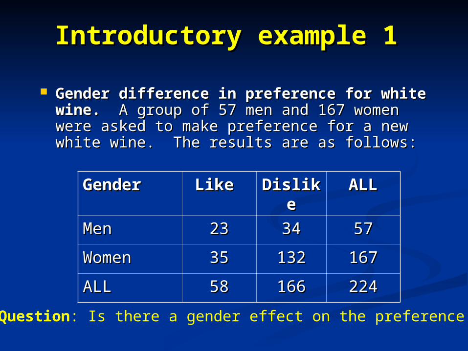
Gender difference in preference for white Gender difference in preference for white wine. wine. A group of 57 men and 167 women A group of 57 men and 167 women were asked to make preference for a new were asked to make preference for a new white wine. The results are as follows:white wine. The results are as follows:

Question: Is there a gender effect on the preference ?

GenderGender Like Like DislikDislikee

ALLALL

MenMen 2323 3434 5757

WomenWomen 3535 132132 167167

ALLALL 5858 166166 224224

Introductory example 2 Introductory example 2 Fat concentration and preference. Fat concentration and preference. 435 samples of a 435 samples of a

sauce of various fat concentration were tasted by sauce of various fat concentration were tasted by consumers. There were two outcome: like or dislike. The consumers. There were two outcome: like or dislike. The results are as follows:results are as follows:

Question: Is there an effect of fat concentration on the preference ?

ConcentratiConcentrationon

Like Like DislikeDislike ALLALL

1.351.35 1313 00 1313

1.601.60 1919 00 1919

1.751.75 6767 22 6969

1.851.85 4545 55 5050

1.951.95 7171 88 7979

2.052.05 5050 2020 7070

2.152.15 3535 3131 6666

2.252.25 77 4949 5656

2.352.35 11 1212 1313

Consideration …Consideration …

The question in example 1 can be addressed by The question in example 1 can be addressed by “traditional” analysis such as z-statistic or Chi-“traditional” analysis such as z-statistic or Chi-square test.square test.

The question in example 2 is a bit difficult to The question in example 2 is a bit difficult to handle as the factor (fat concentration ) was a handle as the factor (fat concentration ) was a continuous variable and the outcome was a continuous variable and the outcome was a categorical variable (like or dislike)categorical variable (like or dislike)

However, there is a much better and more However, there is a much better and more systematic method to analysis these data: systematic method to analysis these data: Logistic regressionLogistic regression

Odds and odds ratioOdds and odds ratio

Let Let PP be the probability of preference, then be the probability of preference, then the the odds of preference odds of preference is: is: O = O = P / (1-P)P / (1-P)

GenderGender Like Like DislikeDislike ALLALL P(like)P(like)

MenMen 2323 3434 5757 0.4030.403

WomenWomen 3535 132132 167167 0.2090.209

ALLALL 5858 166166 224224 0.2590.259

OOmenmen = = 0.403 / 0.597 = 0.6760.403 / 0.597 = 0.676

OOwomenwomen = = 0.209 / 0.791 = 0.2650.209 / 0.791 = 0.265

Odds ratio:Odds ratio: OR = OOR = Omen men / O/ Owomen women = 0.676 / 0.265 = 2.55= 0.676 / 0.265 = 2.55(Meaning: the odds of preference is 2.55 times higher in men than in women)(Meaning: the odds of preference is 2.55 times higher in men than in women)

Meanings of odds ratioMeanings of odds ratio

OR > 1: the odds of preference is higher in OR > 1: the odds of preference is higher in men than in womenmen than in women

OR < 1: the odds of preference is lower in OR < 1: the odds of preference is lower in men than in womenmen than in women

OR = 1: the odds of preference in men is OR = 1: the odds of preference in men is the same as in womenthe same as in women

How to assess the “significance” of How to assess the “significance” of OR ? OR ?

Computing variance of odds Computing variance of odds ratioratio

The significance of OR can be tested by The significance of OR can be tested by calculating its variance.calculating its variance.

The variance of OR can be indirectly The variance of OR can be indirectly calculated by working with logarithmic scale:calculated by working with logarithmic scale: Convert OR to log(OR) Convert OR to log(OR) Calculate variance of log(OR)Calculate variance of log(OR) Calculate 95% confidence interval of log(OR)Calculate 95% confidence interval of log(OR) Convert back to 95% confidence interval of Convert back to 95% confidence interval of

OROR

Computing variance of odds Computing variance of odds ratioratio

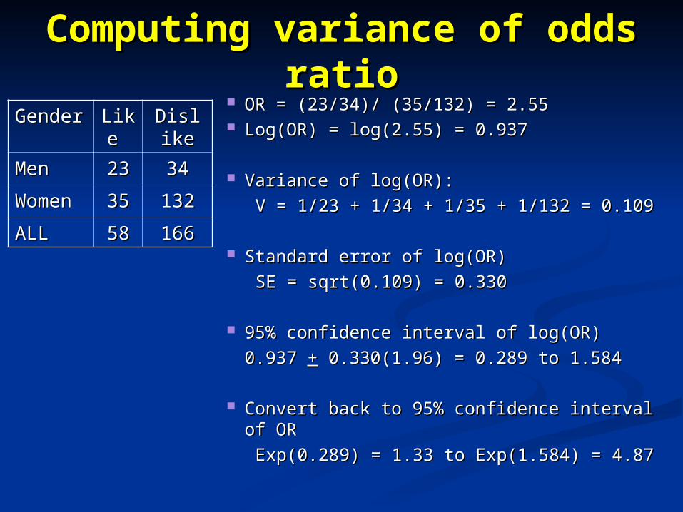
OR = (23/34)/ (35/132) = 2.55OR = (23/34)/ (35/132) = 2.55 Log(OR) = log(2.55) = 0.937Log(OR) = log(2.55) = 0.937

Variance of log(OR): Variance of log(OR):

V = 1/23 + 1/34 + 1/35 + 1/132 = 0.109V = 1/23 + 1/34 + 1/35 + 1/132 = 0.109

Standard error of log(OR)Standard error of log(OR)

SE = sqrt(0.109) = 0.330SE = sqrt(0.109) = 0.330

95% confidence interval of log(OR)95% confidence interval of log(OR)

0.937 0.937 ++ 0.330(1.96) = 0.289 to 1.584 0.330(1.96) = 0.289 to 1.584

Convert back to 95% confidence interval of Convert back to 95% confidence interval of OROR

Exp(0.289) = 1.33 to Exp(1.584) = 4.87Exp(0.289) = 1.33 to Exp(1.584) = 4.87

GenderGender LikLike e

DislikDislikee

MenMen 2323 3434

WomeWomenn

3535 132132

ALLALL 5858 166166

Logistic analysis by RLogistic analysis by Rsex <- c(1, 2)sex <- c(1, 2)

like <- c(23, 35)like <- c(23, 35)

dislike <- c(34, 132)dislike <- c(34, 132)

total <- like + disliketotal <- like + dislike

prob <- like/totalprob <- like/total

logistic <- glm(prob ~ sex, logistic <- glm(prob ~ sex, family=”binomial”, weight=total) family=”binomial”, weight=total)

GenderGender LikLike e

DislikDislikee

MenMen 2323 3434

WomeWomenn

3535 132132

ALLALL 5858 166166> summary(logistic)

Coefficients: Estimate Std. Error z value Pr(>|z|) (Intercept) 0.5457 0.5725 0.953 0.34044 sex -0.9366 0.3302 -2.836 0.00456 **---Signif. codes: 0 '***' 0.001 '**' 0.01 '*' 0.05 '.' 0.1 ' ' 1

(Dispersion parameter for binomial family taken to be 1)

Null deviance: 7.8676e+00 on 1 degrees of freedomResidual deviance: 2.2204e-15 on 0 degrees of freedomAIC: 13.629

Logistic regression model for Logistic regression model for continuous factorcontinuous factor

ConceConcentrationtrationn

Like Like DislikDislikee

% % likelike

1.351.35 1313 00 1.001.00

1.601.60 1919 00 1.001.00

1.751.75 6767 22 0.970.9711

1.851.85 4545 55 0.900.9000

1.951.95 7171 88 0.890.8999

2.052.05 5050 2020 0.710.7144

2.152.15 3535 3131 0.530.5300

2.252.25 77 4949 0.120.1255

2.352.35 11 1212 0.070.0777

0

0.1

0.2

0.3

0.4

0.5

0.6

0.7

0.8

0.9

1

1.35 1.45 1.55 1.65 1.75 1.85 1.95 2.05 2.15 2.25 2.35 2.45

Fat concentration

Pro

babili

ty o

f lik

ing

Analysis by using RAnalysis by using R

conc <- c(1.35, 1.60, 1.75, 1.85, 1.95, 2.05, 2.15, 2.25, 2.35)like <- c(13, 19, 67, 45, 71, 50, 35, 7, 1)dislike <- c(0, 0, 2, 5, 8, 20, 31, 49, 12)

total <- like+dislike

prob <- like/total

plot(prob ~ conc, pch=16, xlab="Concentration")

1.4 1.6 1.8 2.0 2.2

0.2

0.4

0.6

0.8

1.0

Concentration

pro

b

Logistic regression model for Logistic regression model for continuous factor - modelcontinuous factor - model

Let p = probability of preferenceLet p = probability of preference Logit of p is: Logit of p is:

p

pp

1logitlog

Model: Logit(p) = Model: Logit(p) = + + (FAT) (FAT)

where where is the intercept, and is the intercept, and is the slope that is the slope that have to be estimated from the datahave to be estimated from the data

Analysis by using RAnalysis by using Rlogistic <- glm(prob ~ conc, family="binomial",

weight=total)

summary(logistic)

Deviance Residuals: Min 1Q Median 3Q Max -1.78226 -0.69052 0.07981 0.36556 1.36871

Coefficients: Estimate Std. Error z value Pr(>|z|) (Intercept) 22.708 2.266 10.021 <2e-16 ***conc -10.662 1.083 -9.849 <2e-16 ***---Signif. codes: 0 '***' 0.001 '**' 0.01 '*' 0.05 '.' 0.1 ' ' 1

(Dispersion parameter for binomial family taken to be 1)

Null deviance: 198.7115 on 8 degrees of freedomResidual deviance: 8.5568 on 7 degrees of freedomAIC: 37.096

Logistic regression model for Logistic regression model for continuous factor – Interpretationcontinuous factor – Interpretation

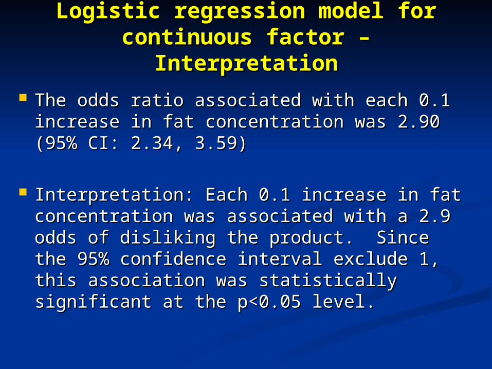
The odds ratio associated with each 0.1 The odds ratio associated with each 0.1 increase in fat concentration was 2.90 (95% increase in fat concentration was 2.90 (95% CI: 2.34, 3.59)CI: 2.34, 3.59)

Interpretation: Each 0.1 increase in fat Interpretation: Each 0.1 increase in fat concentration was associated with a 2.9 concentration was associated with a 2.9 odds of disliking the product. Since the 95% odds of disliking the product. Since the 95% confidence interval exclude 1, this confidence interval exclude 1, this association was statistically significant at association was statistically significant at the p<0.05 level. the p<0.05 level.

Multiple logistic regressionMultiple logistic regression

id fx age bmi bmd ictp pinp 1 1 79 24.7252 0.818 9.170 37.383 2 1 89 25.9909 0.871 7.561 24.685 3 1 70 25.3934 1.358 5.347 40.620 4 1 88 23.2254 0.714 7.354 56.782 5 1 85 24.6097 0.748 6.760 58.358 6 0 68 25.0762 0.935 4.939 67.123 7 0 70 19.8839 1.040 4.321 26.399 8 0 69 25.0593 1.002 4.212 47.515 9 0 74 25.6544 0.987 5.605 26.132 10 0 79 19.9594 0.863 5.204 60.267 ... 137 0 64 38.0762 1.086 5.043 32.835 138 1 80 23.3887 0.875 4.086 23.837 139 0 67 25.9455 0.983 4.328 71.334

Fracture (0=no, 1=yes)

Dependent variables: age, bmi, bmd, ictp, pinp

Question: Which variables are important for fracture?

Multiple logistic regression: R Multiple logistic regression: R analysisanalysis

setwd(“c:/works/stats”)setwd(“c:/works/stats”)fracture <- read.table(“fracture.txt”, fracture <- read.table(“fracture.txt”,

header=TRUE, na.string=”.”)header=TRUE, na.string=”.”)names(fracture) names(fracture) fulldata <- na.omit(fracture)fulldata <- na.omit(fracture)attach(fulldata)attach(fulldata)

temp <- glm(fx ~ ., family=”binomial”, temp <- glm(fx ~ ., family=”binomial”, data=fulldata)data=fulldata)

search <- step(temp)search <- step(temp)summary(search)summary(search)

Bayesian Model Average Bayesian Model Average (BMA) analysis(BMA) analysis

Library(BMA)Library(BMA)xvars <- fulldata[, 3:7]xvars <- fulldata[, 3:7]y <- fxy <- fx

bma.search <- bic.glm(xvars, y, strict=F, bma.search <- bic.glm(xvars, y, strict=F, OR=20, glm.family="binomial") OR=20, glm.family="binomial")

summary(bma.search) summary(bma.search)

imageplot.bma(bma.search) imageplot.bma(bma.search)

Bayesian Model Average Bayesian Model Average (BMA) analysis(BMA) analysis

> summary(bma.search) > summary(bma.search) Call:Call:

Best 5 models (cumulative posterior probability = 0.8836 ): Best 5 models (cumulative posterior probability = 0.8836 ):

p!=0 EV SD model 1 model 2 model 3 model 4 model 5 p!=0 EV SD model 1 model 2 model 3 model 4 model 5 Intercept 100 -2.85012 2.8651 -3.920 -1.065 -1.201 -8.257 -0.072Intercept 100 -2.85012 2.8651 -3.920 -1.065 -1.201 -8.257 -0.072age 15.3 0.00845 0.0261 . . . 0.063 . age 15.3 0.00845 0.0261 . . . 0.063 . bmi 21.7 -0.02302 0.0541 . . -0.116 . -0.070bmi 21.7 -0.02302 0.0541 . . -0.116 . -0.070bmd 39.7 -1.34136 1.9762 . -3.499 . . -2.696bmd 39.7 -1.34136 1.9762 . -3.499 . . -2.696ictp 100.0 0.64575 0.1699 0.606 0.687 0.680 0.554 0.714ictp 100.0 0.64575 0.1699 0.606 0.687 0.680 0.554 0.714pinp 5.7 -0.00037 0.0041 . . . . . pinp 5.7 -0.00037 0.0041 . . . . . nVar 1 2 2 2 3 nVar 1 2 2 2 3 BIC -525.044 -524.939 -523.625 -522.672 -521.032BIC -525.044 -524.939 -523.625 -522.672 -521.032post prob 0.307 0.291 0.151 0.094 0.041post prob 0.307 0.291 0.151 0.094 0.041

Bayesian Model Average Bayesian Model Average (BMA) analysis(BMA) analysis

> imageplot.bma(bma.search)> imageplot.bma(bma.search)

Models selected by BMA

Model #

1 2 3 4 5 7 9

pinp

ictp

bmd

bmi

age

Summary of main pointsSummary of main points

Logistic regression model is used to Logistic regression model is used to analyze the association between a analyze the association between a binary binary outcome outcome and one or many and one or many determinantsdeterminants..

The determinants can be binary, The determinants can be binary, categorical or continuous measurementscategorical or continuous measurements

The model is logit(p) = log[p / (1-p)] = The model is logit(p) = log[p / (1-p)] = + + X, where X is a factor, and X, where X is a factor, and and and must be estimated from observed data.must be estimated from observed data.

Summary of main pointsSummary of main points

Exp(Exp() is the odds ratio associated with ) is the odds ratio associated with an increment in the determinant X.an increment in the determinant X.

The logistic regression model can be The logistic regression model can be extended to include many determinants: extended to include many determinants:

logit(p) = log[p / (1-p)] = logit(p) = log[p / (1-p)] = + + XX11 + + XX22 + + XX33 + … + …