introduction to fluid mechanics simulation using the...
TRANSCRIPT
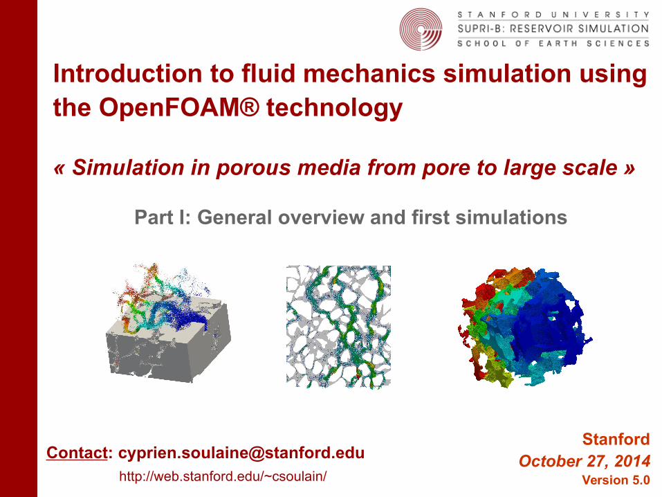
Introduction to fluid mechanics simulation using the OpenFOAM® technology
« Simulation in porous media from pore to large scale »
Part I: General overview and first simulations
StanfordOctober 27, 2014
Version 5.0
Contact: [email protected]://web.stanford.edu/~csoulain/
Op
enF
OA
M®
initi
atio
nObjectives
• Have an overview of the OpenFOAM® capabilities
• Be able to find help and documentation
• Know how to start and post-treat a simulation from existing tutorials
• Start your own simulation by modifying existing tutorials
• Understand what is behind solvers to identify the most suitable for the specific problem
• Program your own solver by modifying an existing solver
• Join the OpenFOAM® adventure…
Op
enF
OA
M®
initi
atio
n
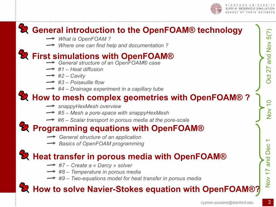
General introduction to the OpenFOAM® technologyWhat is OpenFOAM ?
First simulations with OpenFOAM®
#1 – Heat diffusionGeneral structure of an OpenFOAM® case
#2 – Cavity
Where one can find help and documentation ?
#3 – Poiseuille flow#4 – Drainage experiment in a capillary tube
How to mesh complex geometries with OpenFOAM® ?
#5 – Mesh a pore-space with snappyHexMeshsnappyHexMesh overview
#6 – Scalar transport in porous media at the pore-scale
Programming equations with OpenFOAM®
Basics of OpenFOAM programmingGeneral structure of an application
Heat transfer in porous media with OpenFOAM®
#8 – Temperature in porous media#7 – Create a « Darcy » solver
#9 – Two-equations model for heat transfer in porous media
How to solve Navier-Stokes equation with OpenFOAM®?
Oc t
27
a nd
No v
5(?
)N
o v 1
0N
o v 1
7 a n
d D
ec 1
Op
enF
OA
M®
initi
atio
n
General introduction to the OpenFOAM® technologyWhat is OpenFOAM ?
First simulations with OpenFOAM®
#1 – Heat diffusionGeneral structure of an OpenFOAM® case
#2 – Cavity
Where one can find help and documentation ?
#3 – Poiseuille flow#4 – Drainage experiment in a capillary tube
How to mesh complex geometries with OpenFOAM® ?
#5 – Mesh a pore-space with snappyHexMeshsnappyHexMesh overview
#6 – Scalar transport in porous media at the pore-scale
Programming equations with OpenFOAM®
Basics of OpenFOAM programmingGeneral structure of an application
Heat transfer in porous media with OpenFOAM®
#8 – Temperature in porous media#7 – Create a « Darcy » solver
#9 – Two-equations model for heat transfer in porous media
How to solve Navier-Stokes equation with OpenFOAM® ?
Op
enF
OA
M®
initi
atio
n
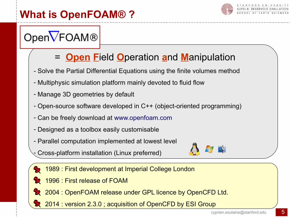
1989 : First development at Imperial College London
1996 : First release of FOAM
2004 : OpenFOAM release under GPL licence by OpenCFD Ltd.
2014 : version 2.3.0 ; acquisition of OpenCFD by ESI Group
= Open Field Operation and Manipulation- Solve the Partial Differential Equations using the finite volumes method
- Multiphysic simulation platform mainly devoted to fluid flow
- Manage 3D geometries by default
- Open-source software developed in C++ (object-oriented programming)
- Can be freely download at www.openfoam.com
- Designed as a toolbox easily customisable
- Parallel computation implemented at lowest level
- Cross-platform installation (Linux preferred)
What is OpenFOAM® ?
Op
enF
OA
M®
initi
atio
nThe OpenFOAM® toolbox
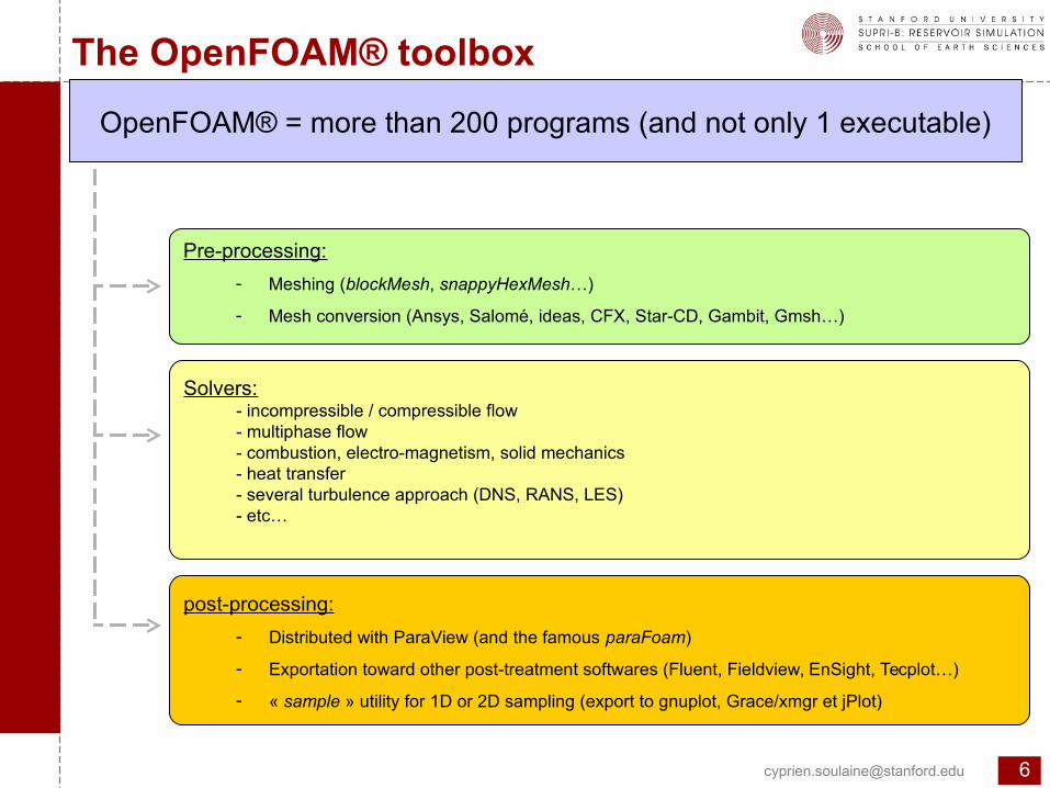
OpenFOAM® = more than 200 programs (and not only 1 executable)
post-processing:
- Distributed with ParaView (and the famous paraFoam)
- Exportation toward other post-treatment softwares (Fluent, Fieldview, EnSight, Tecplot…)
- « sample » utility for 1D or 2D sampling (export to gnuplot, Grace/xmgr et jPlot)
Solvers:- incompressible / compressible flow- multiphase flow- combustion, electro-magnetism, solid mechanics- heat transfer- several turbulence approach (DNS, RANS, LES)- etc…
Pre-processing:
- Meshing (blockMesh, snappyHexMesh…)
- Mesh conversion (Ansys, Salomé, ideas, CFX, Star-CD, Gambit, Gmsh…)
Op
enF
OA
M®
initi
atio
n
op
en
foa
m.c
om
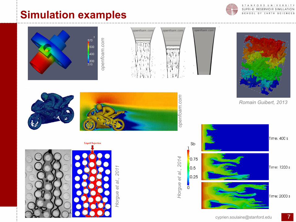
Simulation examples
Romain Guibert, 2013
Ho
rgu
e e
t a
l. , 2
01 1
op
en
foa
m.c
om
Ho
rgu
e e
t a
l. , 2
01
4
Op
enF
OA
M®
initi
atio
nPorous media modeling with OpenFOAM
P. Horgue, C. Soulaine, J. Franc, R. Guibert, G. Debenest, An open-source toolbox for multiphase flow in porous media, Computer Physics Communications (2014)
L. Orgogozo, N. Renon, C. Soulaine, F. Hénon, S. K. Tomer, D. Labat, O. S. Pokrovsky, M. Sekhar, R. Ababou, M. Quintard, An open source massively parallel solver for Richards equation: Mechanistic modelling of water fluxes at the watershed scale, Computer Physics Communications 185 (2014) 3358–3371
http://cpc.cs.qub.ac.uk/summaries/AEUF_v1_0.html
P. Horgue, F. Augier, P. Duru, M. Prat, M. Quintard, Experimental and numerical study of two-phase flows in arrays of cylinders, Chemical Engineering Science 102 (2013) 335 - 345
C. Soulaine, M. Quintard, H. Allain, B. Baudouy, R. Van Weelderen, A PISO-like algorithm to simulate superfluid helium flow with the two-fluid model, Computer Physics Communications (2014)
Shewani, A., Horgue, P., Pommier, S., Debenest, G., Lefebvre, X., Gandon, E., Paul, E., Assessment of percolation through a solid leach bed in dry batch anaerobic digestion processes, Bioresource Technology (2014)
C. Soulaine, P. Horgue, J. Franc, M. Quintard, Gas–Liquid Flow Modeling in Columns Equipped with Structured Packing, AIChE Journal 60 (2014) 3665-3674
https://github.com/phorgue/porousMultiphaseFoam.git
Multiphase flow simulation in porous media at Darcy-scale
Immiscible two-phase at pore-scale
Digital Rock Physics with OpenFOAMR. Guibert, P. Creux, M. Quintard, Permeability calculation from DNS simulations, Transport in Porous Media (in press)
Superfluid helium flow in porous media at pore-scale
Op
enF
OA
M®
initi
atio
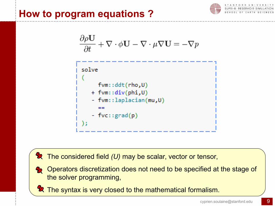
nHow to program equations ?
The considered field (U) may be scalar, vector or tensor,
Operators discretization does not need to be specified at the stage of the solver programming,
The syntax is very closed to the mathematical formalism.
Op
enF
OA
M®
initi
atio
n
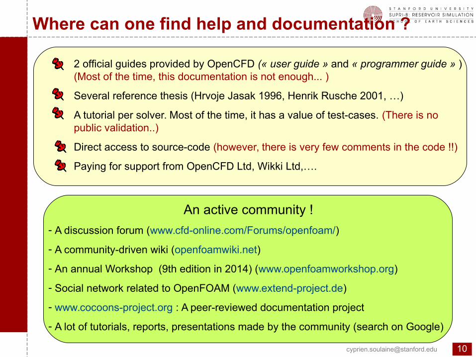
2 official guides provided by OpenCFD (« user guide » and « programmer guide » ) (Most of the time, this documentation is not enough... )
Several reference thesis (Hrvoje Jasak 1996, Henrik Rusche 2001, …)
A tutorial per solver. Most of the time, it has a value of test-cases. (There is no public validation..)
Direct access to source-code (however, there is very few comments in the code !!)
Paying for support from OpenCFD Ltd, Wikki Ltd,….
An active community !
- A discussion forum (www.cfd-online.com/Forums/openfoam/)
- A community-driven wiki (openfoamwiki.net)
- An annual Workshop (9th edition in 2014) (www.openfoamworkshop.org)
- Social network related to OpenFOAM (www.extend-project.de)
- www.cocoons-project.org : A peer-reviewed documentation project
- A lot of tutorials, reports, presentations made by the community (search on Google)
Where can one find help and documentation ?
Op
enF
OA
M®
initi
atio
n
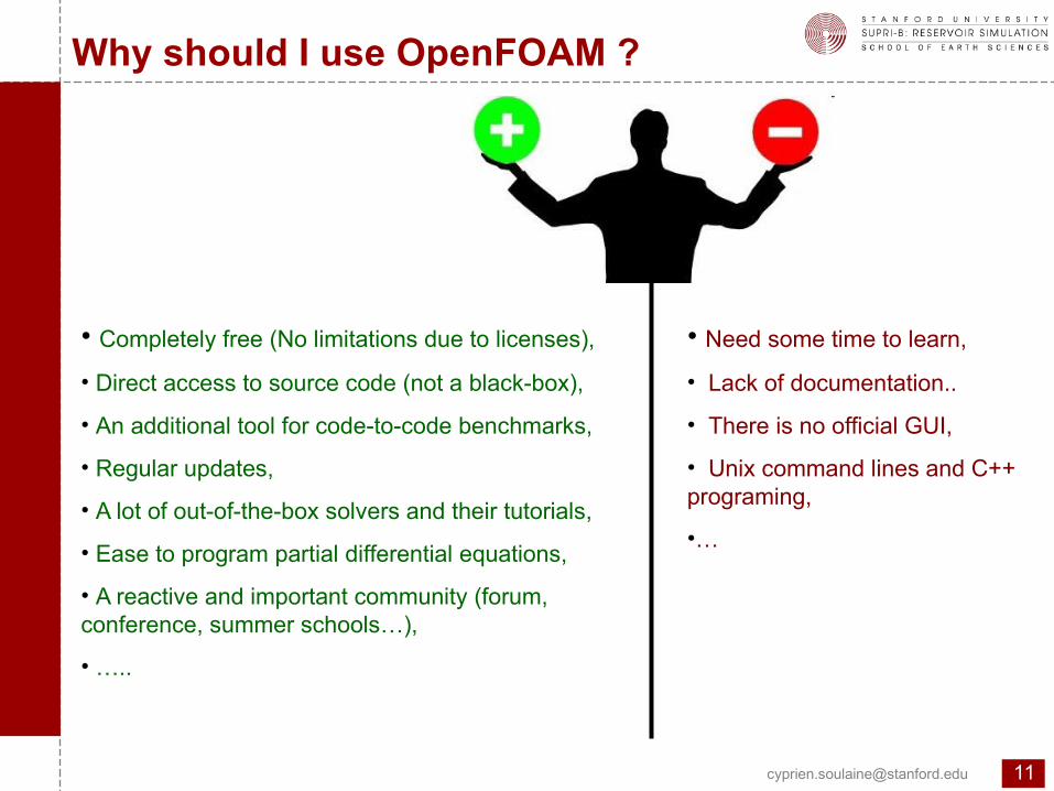
• Completely free (No limitations due to licenses),
• Direct access to source code (not a black-box),
• An additional tool for code-to-code benchmarks,
• Regular updates,
• A lot of out-of-the-box solvers and their tutorials,
• Ease to program partial differential equations,
• A reactive and important community (forum, conference, summer schools…),
• …..
• Need some time to learn,
• Lack of documentation..
• There is no official GUI,
• Unix command lines and C++ programing,
•…
Why should I use OpenFOAM ?
Op
enF
OA
M®
initi
atio
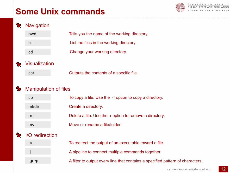
nSome Unix commands
Navigation
pwd Tells you the name of the working directory.
ls List the files in the working directory.
cd Change your working directory.
Manipulation of files
cp To copy a file. Use the -r option to copy a directory.
mkdir Create a directory.
rm Delete a file. Use the -r option to remove a directory.
mv Move or rename a file/folder.
I/O redirection
> To redirect the output of an executable toward a file.
| A pipeline to connect multiple commands together.
grep A filter to output every line that contains a specified pattern of characters.
Visualization
cat Outputs the contents of a specific file.
Op
enF
OA
M®
initi
atio
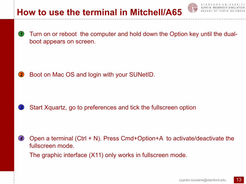
nHow to use the terminal in Mitchell/A65
Turn on or reboot the computer and hold down the Option key until the dual-boot appears on screen.
1
2
3
Boot on Mac OS and login with your SUNetID.
Start Xquartz, go to preferences and tick the fullscreen option
4 Open a terminal (Ctrl + N). Press Cmd+Option+A to activate/deactivate the fullscreen mode.
The graphic interface (X11) only works in fullscreen mode.
Op
enF
OA
M®
initi
atio
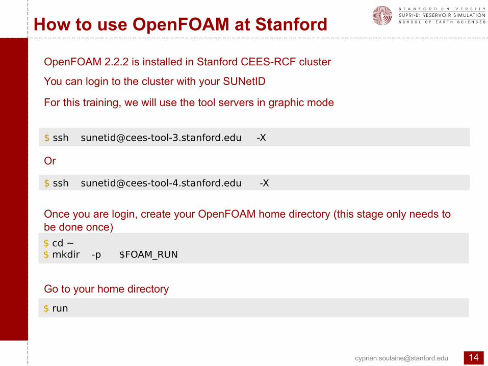
nHow to use OpenFOAM at Stanford
OpenFOAM 2.2.2 is installed in Stanford CEES-RCF cluster
You can login to the cluster with your SUNetID
$ ssh [email protected] -X
$ ssh [email protected] -X
For this training, we will use the tool servers in graphic mode
Or
Once you are login, create your OpenFOAM home directory (this stage only needs to be done once)
$ cd ~$ mkdir -p $FOAM_RUN
Go to your home directory
$ run
Op
enF
OA
M®
initi
atio
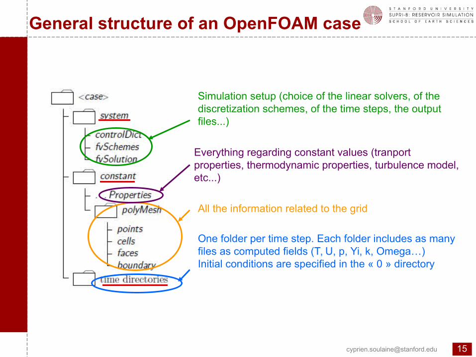
nGeneral structure of an OpenFOAM case
Simulation setup (choice of the linear solvers, of the discretization schemes, of the time steps, the output files...)
All the information related to the grid
Everything regarding constant values (tranport properties, thermodynamic properties, turbulence model, etc...)
One folder per time step. Each folder includes as many files as computed fields (T, U, p, Yi, k, Omega…)Initial conditions are specified in the « 0 » directory
Op
enF
OA
M®
initi
atio
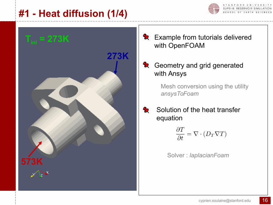
n#1 - Heat diffusion (1/4)
Geometry and grid generated with Ansys
Solution of the heat transfer equation
Mesh conversion using the utilityansysToFoam
Example from tutorials delivered with OpenFOAM
573K
273K
Tini = 273K
Solver : laplacianFoam
Op
enF
OA
M®
initi
atio
n#1 - Heat diffusion (2/4)
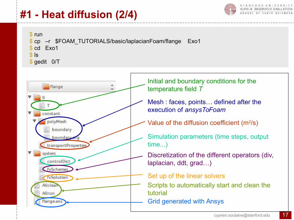
$ run $ cp –r $FOAM_TUTORIALS/basic/laplacianFoam/flange Exo1 $ cd Exo1 $ ls $ gedit 0/T
Initial and boundary conditions for the temperature field T
Mesh : faces, points… defined after the execution of ansysToFoam
Value of the diffusion coefficient (m2/s)
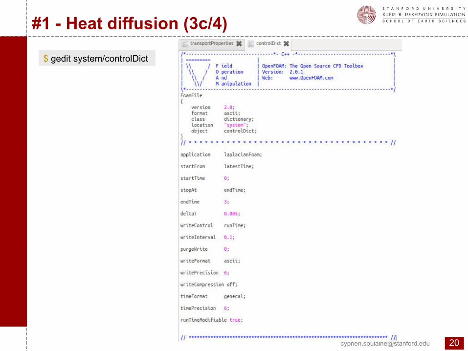
Simulation parameters (time steps, output time...)
Discretization of the different operators (div, laplacian, ddt, grad…)
Set up of the linear solvers
Scripts to automatically start and clean the tutorialGrid generated with Ansys
Op
enF
OA
M®
initi
atio
n#1 - Heat diffusion (3a/4)
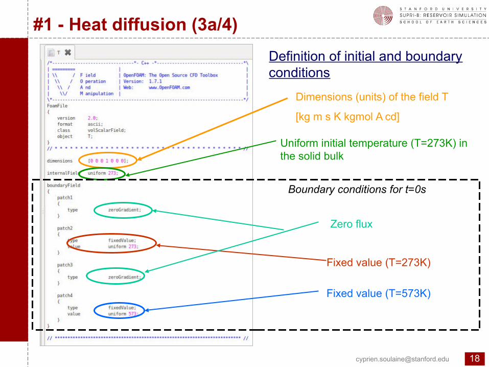
Definition of initial and boundary conditions
Dimensions (units) of the field T
[kg m s K kgmol A cd]
Uniform initial temperature (T=273K) in the solid bulk
Fixed value (T=273K)
Zero flux
Fixed value (T=573K)
Boundary conditions for t=0s
Op
enF
OA
M®
initi
atio
n#1 - Heat diffusion (3b/4)
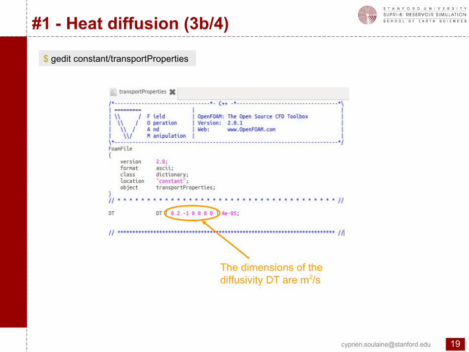
$ gedit constant/transportProperties
The dimensions of the diffusivity DT are m2/s
Op
enF
OA
M®
initi
atio
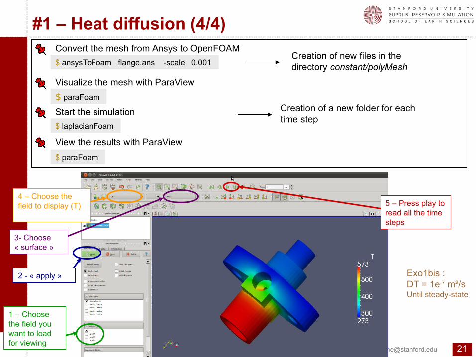
n#1 – Heat diffusion (4/4)
Convert the mesh from Ansys to OpenFOAM
$ ansysToFoam flange.ans -scale 0.001
Visualize the mesh with ParaView
$ paraFoam
Start the simulation
$ laplacianFoam
View the results with ParaView
$ paraFoam
Creation of new files in the directory constant/polyMesh
Creation of a new folder for each time step
1 – Choose the field you want to load for viewing
2 - « apply »
3- Choose « surface »
4 – Choose the field to display (T) 5 – Press play to
read all the time steps
Exo1bis : DT = 1e-7 m²/sUntil steady-state
Op
enF
OA
M®
initi
atio
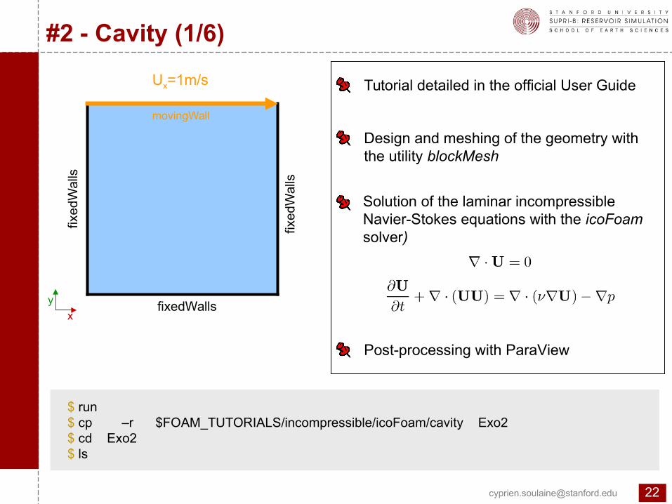
n#2 - Cavity (1/6)
Design and meshing of the geometry with the utility blockMesh
Solution of the laminar incompressible Navier-Stokes equations with the icoFoam solver)
Post-processing with ParaView
$ run $ cp –r $FOAM_TUTORIALS/incompressible/icoFoam/cavity Exo2$ cd Exo2 $ ls
Tutorial detailed in the official User Guide
fixedWalls
fixed
Wal
ls
fixed
Wal
ls
Ux=1m/s
movingWall
x
y
Op
enF
OA
M®
initi
atio
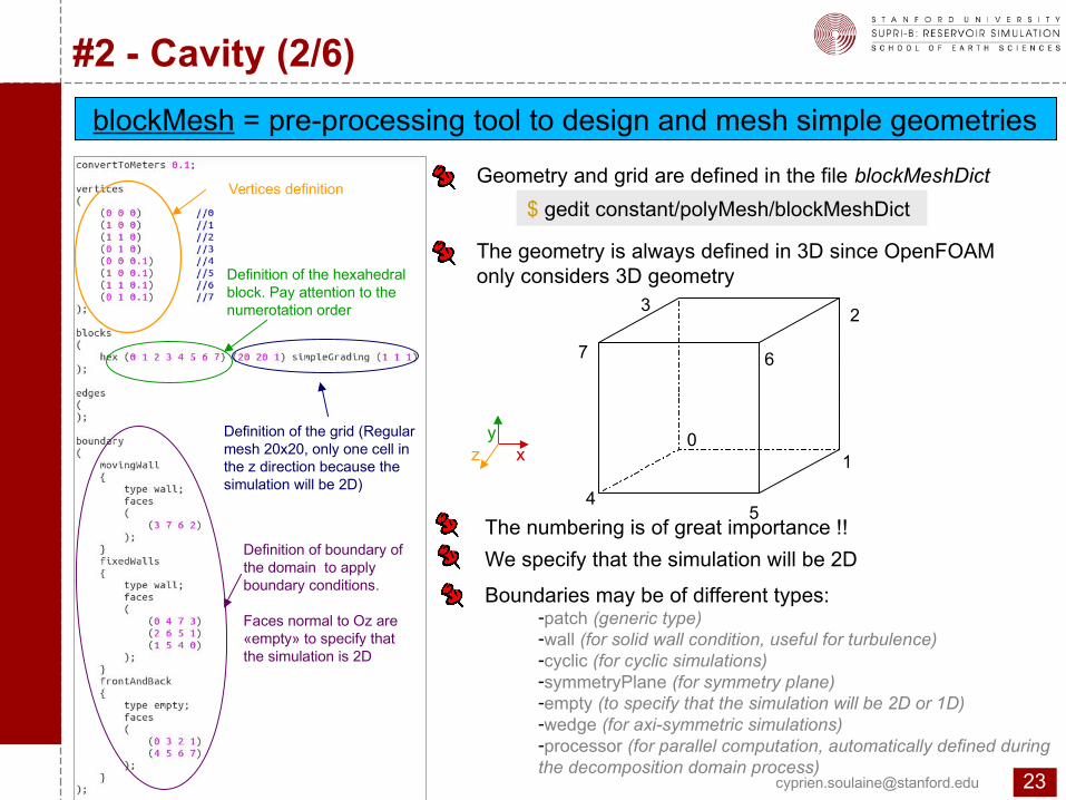
n#2 - Cavity (2/6)
Geometry and grid are defined in the file blockMeshDict
$ gedit constant/polyMesh/blockMeshDict
blockMesh = pre-processing tool to design and mesh simple geometries
The geometry is always defined in 3D since OpenFOAM only considers 3D geometry
45
67
32
10
xy
z
The numbering is of great importance !!
Vertices definition
Definition of the hexahedral block. Pay attention to the numerotation order
Definition of the grid (Regular mesh 20x20, only one cell in the z direction because the simulation will be 2D)
Definition of boundary of the domain to apply boundary conditions.
Faces normal to Oz are «empty» to specify that the simulation is 2D
We specify that the simulation will be 2D
Boundaries may be of different types: -patch (generic type)-wall (for solid wall condition, useful for turbulence)-cyclic (for cyclic simulations)-symmetryPlane (for symmetry plane)-empty (to specify that the simulation will be 2D or 1D)-wedge (for axi-symmetric simulations)-processor (for parallel computation, automatically defined during the decomposition domain process)
Op
enF
OA
M®
initi
atio
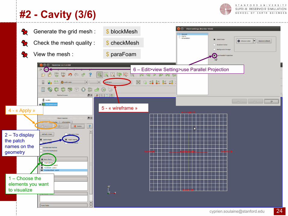
n#2 - Cavity (3/6)
Generate the grid mesh : $ blockMesh
Check the mesh quality : $ checkMesh
View the mesh : $ paraFoam
1 – Choose the elements you want to visualize
2 – To display the patch names on the geometry
4 - « Apply » 5 - « wireframe »
6 – Edit>view Setting>use Parallel Projection
Op
enF
OA
M®
initi
atio
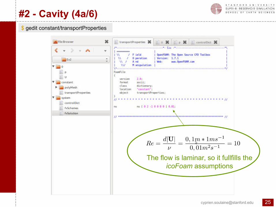
n#2 - Cavity (4a/6)$ gedit constant/transportProperties
The flow is laminar, so it fullfills the icoFoam assumptions
Op
enF
OA
M®
initi
atio
n
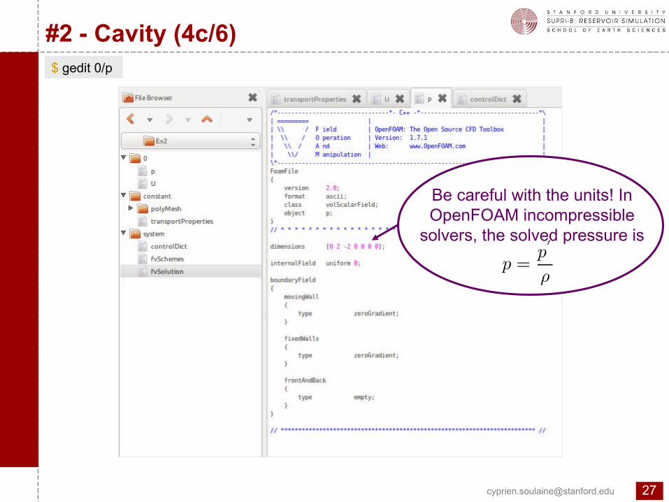
$ gedit 0/p
#2 - Cavity (4c/6)
Be careful with the units! In OpenFOAM incompressible
solvers, the solved pressure is
Op
enF
OA
M®
initi
atio
n
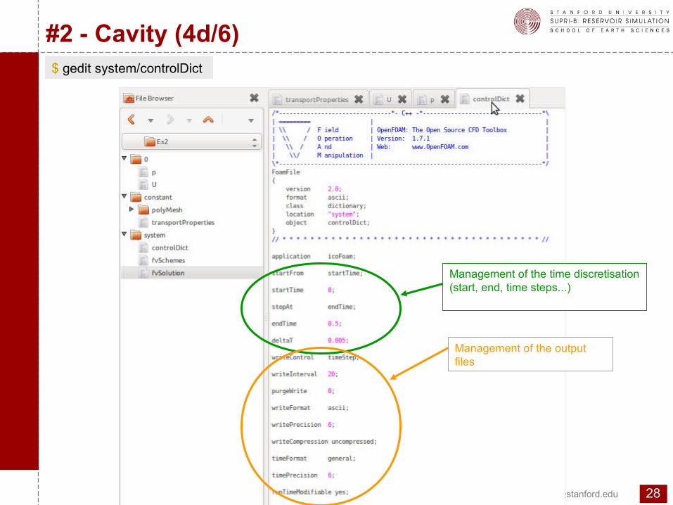
$ gedit system/controlDict
#2 - Cavity (4d/6)
Management of the time discretisation (start, end, time steps...)
Management of the output files
Op
enF
OA
M®
initi
atio
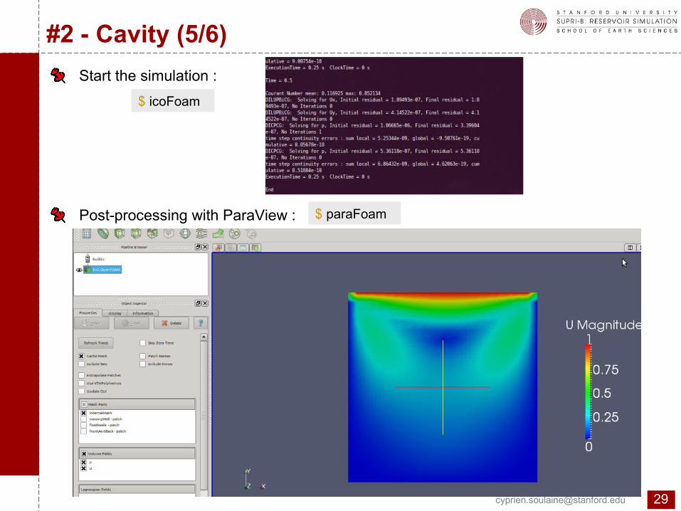
n#2 - Cavity (5/6)
Start the simulation :
$ icoFoam
Post-processing with ParaView : $ paraFoam
Op
enF
OA
M®
initi
atio
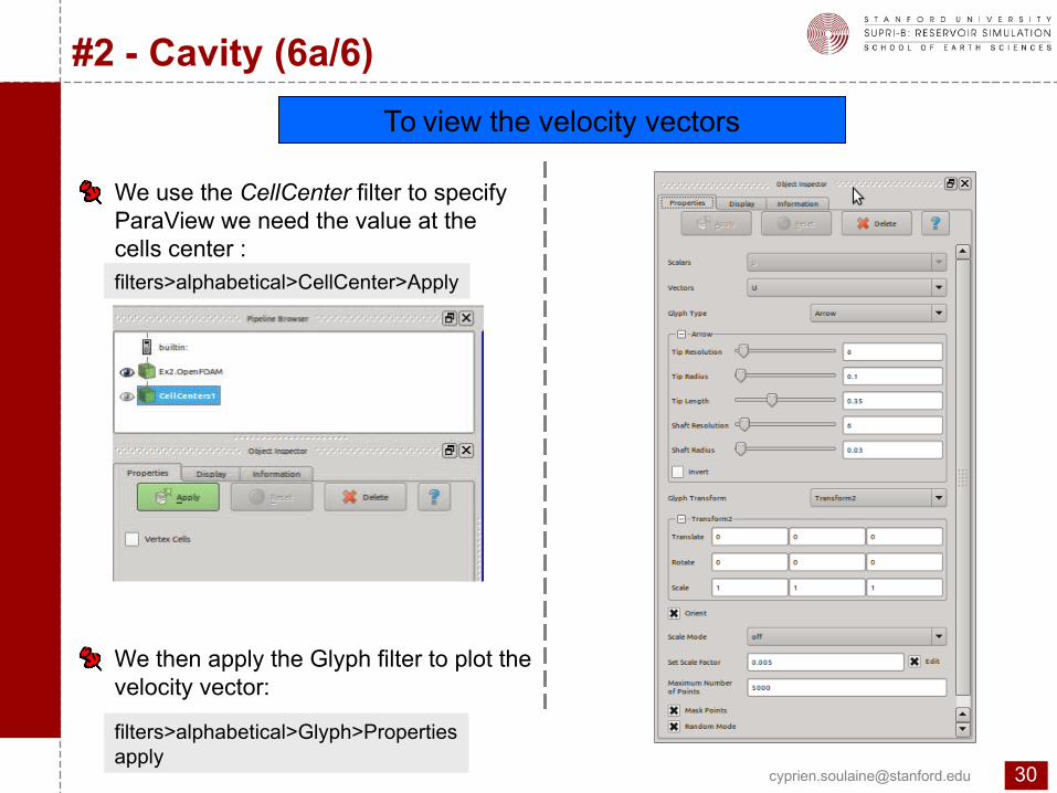
n#2 - Cavity (6a/6)
We use the CellCenter filter to specify ParaView we need the value at the cells center :filters>alphabetical>CellCenter>Apply
To view the velocity vectors
We then apply the Glyph filter to plot the velocity vector:
filters>alphabetical>Glyph>Propertiesapply
Op
enF
OA
M®
initi
atio
n
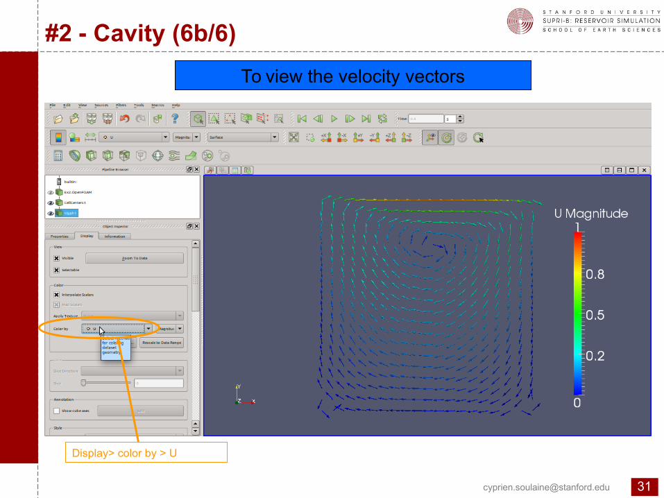
To view the velocity vectors
#2 - Cavity (6b/6)
Display> color by > U
Op
enF
OA
M®
initi
atio
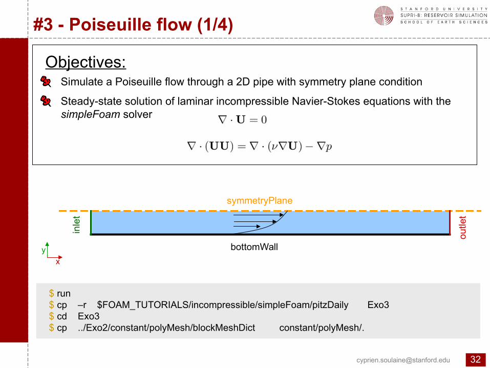
n#3 - Poiseuille flow (1/4)
Simulate a Poiseuille flow through a 2D pipe with symmetry plane condition
Steady-state solution of laminar incompressible Navier-Stokes equations with the simpleFoam solver
$ run $ cp –r $FOAM_TUTORIALS/incompressible/simpleFoam/pitzDaily Exo3 $ cd Exo3 $ cp ../Exo2/constant/polyMesh/blockMeshDict constant/polyMesh/.
Objectives:
x
y bottomWall
symmetryPlane
outle
t
inle
t
Op
enF
OA
M®
initi
atio
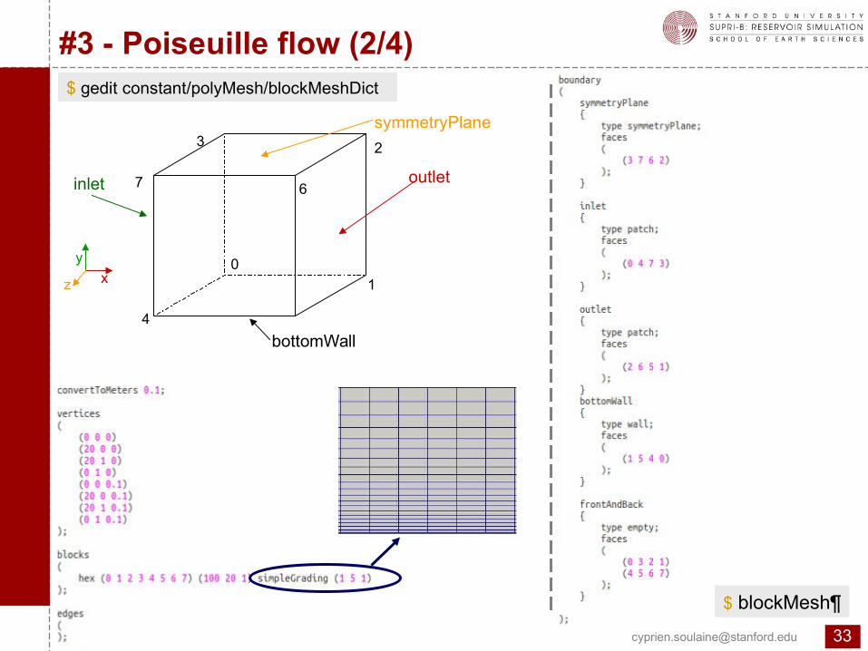
n#3 - Poiseuille flow (2/4)$ gedit constant/polyMesh/blockMeshDict
4
67
3 2
1
0x
y
z
inlet
bottomWall
outlet
symmetryPlane
$ blockMesh
Op
enF
OA
M®
initi
atio
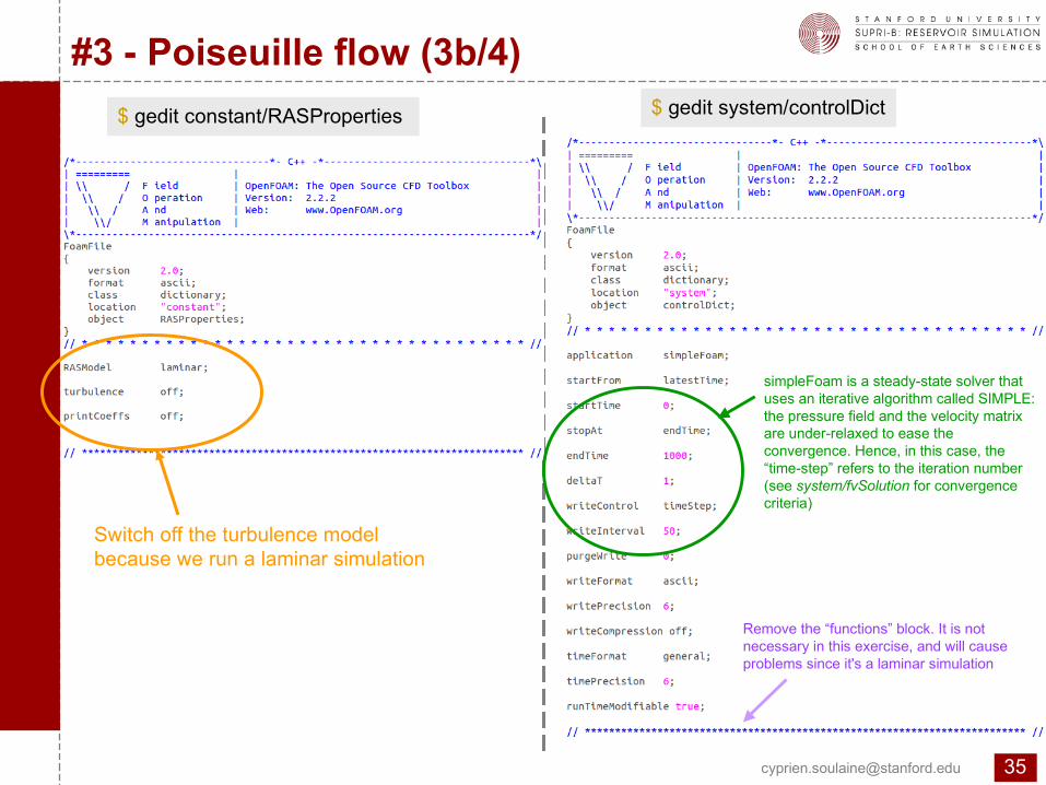
n#3 - Poiseuille flow (3b/4)
$ gedit constant/RASProperties $ gedit system/controlDict
Switch off the turbulence model because we run a laminar simulation
simpleFoam is a steady-state solver that uses an iterative algorithm called SIMPLE: the pressure field and the velocity matrix are under-relaxed to ease the convergence. Hence, in this case, the “time-step” refers to the iteration number (see system/fvSolution for convergence criteria)
Remove the “functions” block. It is not necessary in this exercise, and will cause problems since it's a laminar simulation
Op
enF
OA
M®
initi
atio
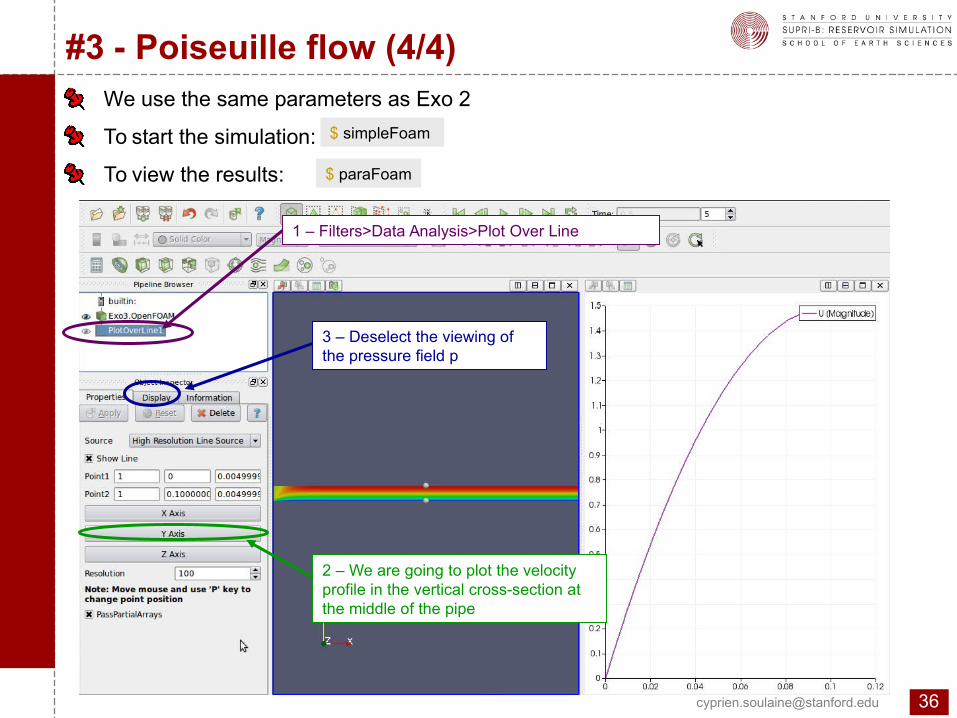
n#3 - Poiseuille flow (4/4)
To start the simulation: $ simpleFoam
To view the results: $ paraFoam
1 – Filters>Data Analysis>Plot Over Line
2 – We are going to plot the velocity profile in the vertical cross-section at the middle of the pipe
3 – Deselect the viewing of the pressure field p
We use the same parameters as Exo 2
Op
enF
OA
M®
initi
atio
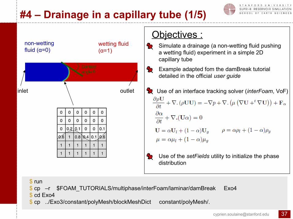
n#4 – Drainage in a capillary tube (1/5)
$ run $ cp –r $FOAM_TUTORIALS/multiphase/interFoam/laminar/damBreak Exo4 $ cd Exo4 $ cp ../Exo3/constant/polyMesh/blockMeshDict constant/polyMesh/.
Simulate a drainage (a non-wetting fluid pushing a wetting fluid) experiment in a simple 2D capillary tube
Use of an interface tracking solver (interFoam, VoF)
Use of the setFields utility to initialize the phase distribution
Objectives :
Example adapted fom the damBreak tutorial detailed in the official user guide
non-wetting fluid (α=0)
outletinlet
wetting fluid (α=1)
Contact angle θ
Op
enF
OA
M®
initi
atio
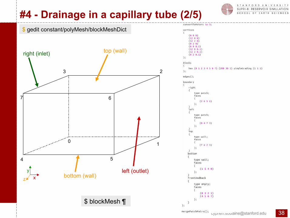
n#4 - Drainage in a capillary tube (2/5)$ gedit constant/polyMesh/blockMeshDict
4
67
3 2
10
x
y
z
top (wall)
left (outlet)
$ blockMesh 
right (inlet)
bottom (wall)
5
Op
enF
OA
M®
initi
atio
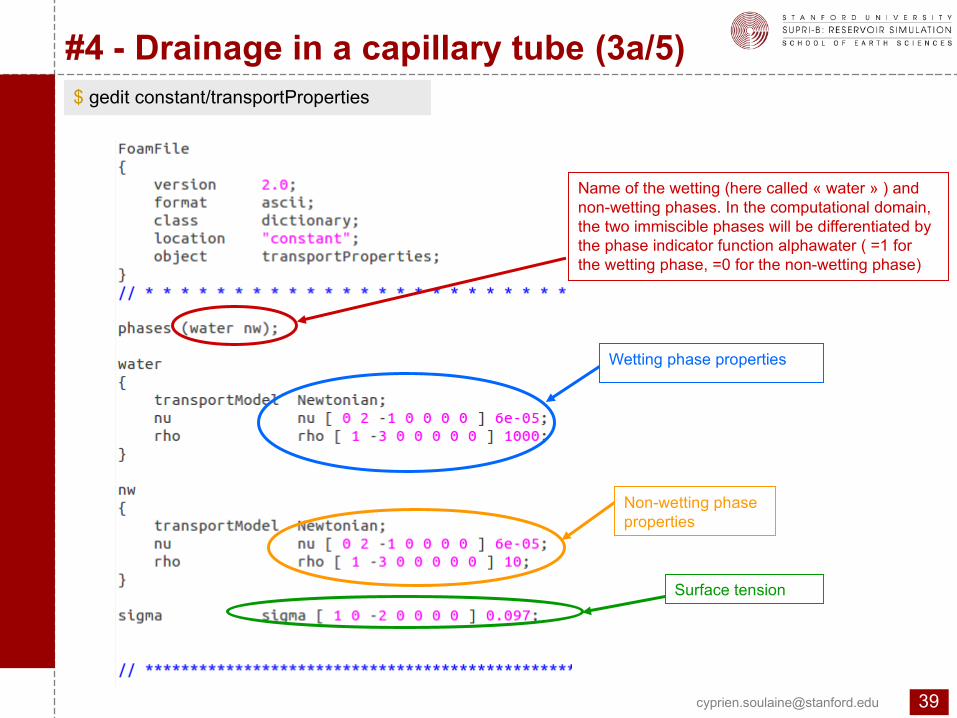
n#4 - Drainage in a capillary tube (3a/5)$ gedit constant/transportProperties
Wetting phase properties
Non-wetting phase properties
Surface tension
Name of the wetting (here called « water » ) and non-wetting phases. In the computational domain, the two immiscible phases will be differentiated by the phase indicator function alphawater ( =1 for the wetting phase, =0 for the non-wetting phase)
Op
enF
OA
M®
initi
atio
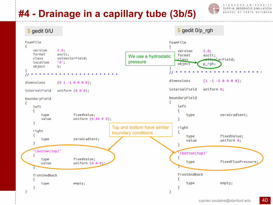
n#4 - Drainage in a capillary tube (3b/5)
$ gedit 0/U $ gedit 0/p_rgh
We use a hydrostatic pressure
Top and bottom have similar boundary conditions
Op
enF
OA
M®
initi
atio
n#4 - Drainage in a capillary tube (3c/5)
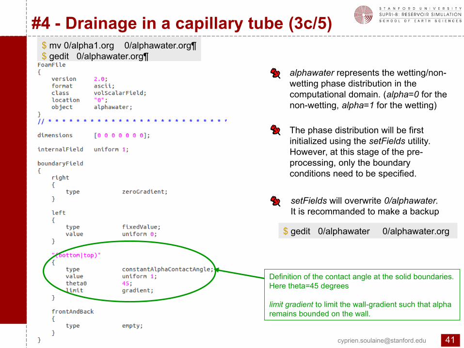
$ mv 0/alpha1.org 0/alphawater.org¶$ gedit 0/alphawater.org
alphawater represents the wetting/non-wetting phase distribution in the computational domain. (alpha=0 for the non-wetting, alpha=1 for the wetting)
The phase distribution will be first initialized using the setFields utility. However, at this stage of the pre-processing, only the boundary conditions need to be specified.
setFields will overwrite 0/alphawater. It is recommanded to make a backup
Definition of the contact angle at the solid boundaries. Here theta=45 degrees
limit gradient to limit the wall-gradient such that alpha remains bounded on the wall.
$ gedit 0/alphawater 0/alphawater.org
Op
enF
OA
M®
initi
atio
n#4 - Drainage in a capillary tube (3d/5)
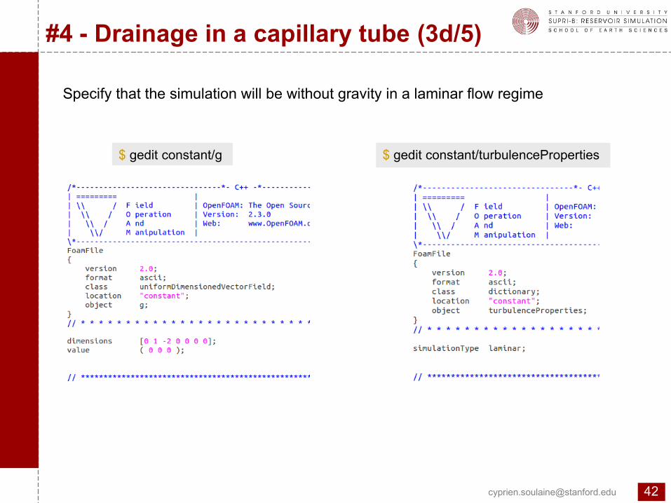
$ gedit constant/g $ gedit constant/turbulenceProperties
Specify that the simulation will be without gravity in a laminar flow regime
Op
enF
OA
M®
initi
atio
n#4 - Drainage in a capillary tube (3e/5)
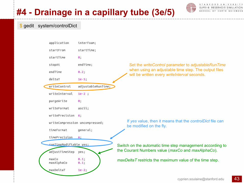
$ gedit system/controlDict
Set the writeControl parameter to adjustableRunTime when using an adjustable time step. The output files will be written every writeInterval seconds.
Switch on the automatic time step management according to the Courant Numbers value (maxCo and maxAlphaCo).
maxDeltaT restricts the maximum value of the time step.
If yes value, then it means that the controlDict file can be modified on the fly.
Op
enF
OA
M®
initi
atio
n#4 - Drainage in a capillary tube (4/5)
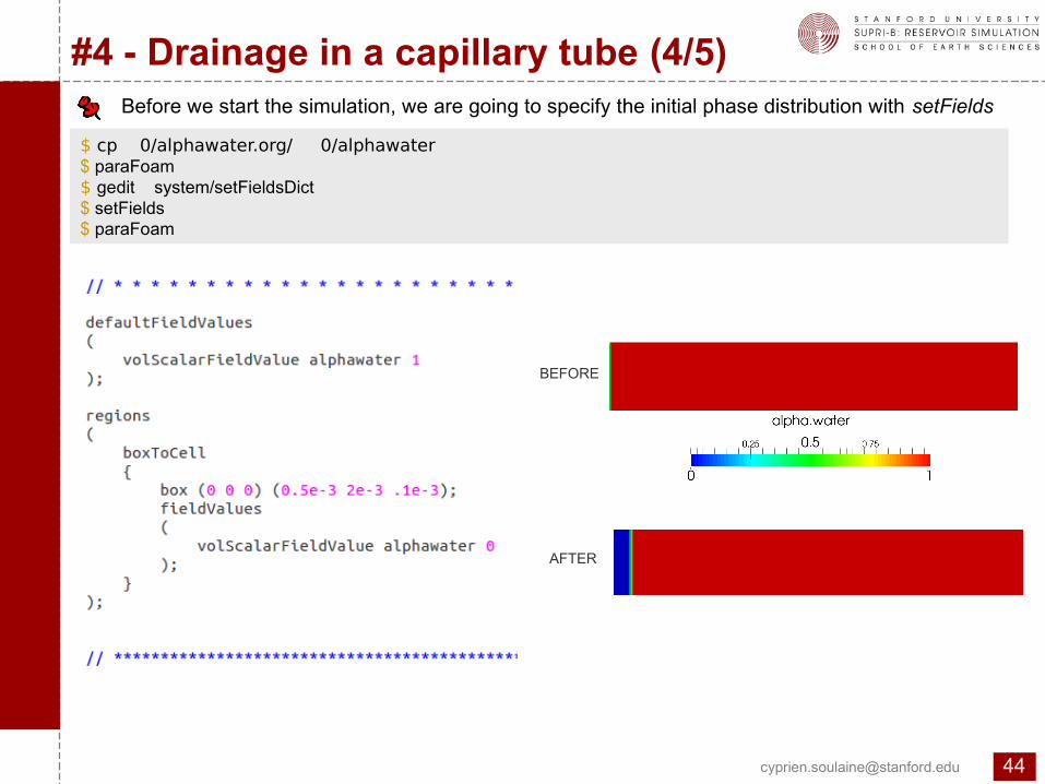
BEFORE
Before we start the simulation, we are going to specify the initial phase distribution with setFields
$ cp 0/alphawater.org/ 0/alphawater $ paraFoam $ gedit system/setFieldsDict $ setFields $ paraFoam
AFTER
Op
enF
OA
M®
initi
atio
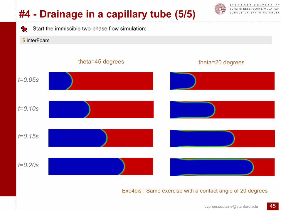
n#4 - Drainage in a capillary tube (5/5)
$ interFoam
Start the immiscible two-phase flow simulation:
t=0.05s
t=0.10s
t=0.15s
t=0.20s
Exo4bis : Same exercise with a contact angle of 20 degrees
theta=45 degrees theta=20 degrees
Op
enF
OA
M®
initi
atio
nIn the next parts...
Part II: Mesh complex geometries, application to the evaluation of permeability, transport of passive scalars at the pore-scale
Part III: First programs, development of a heat tranfer solver in porous media
http://web.stanford.edu/~csoulain/