Introduction to

Artificial Neural Networks

Introduction based on the Bachelor Thesis of Marius Felix Killinger (2014)

Contents

1 Artificial Neural Networks 4

1.1 Origin and Motivation . . . . . . . . . . . . . . . . . . . . . . . . . . . . . 4

1.2 Biological Background . . . . . . . . . . . . . . . . . . . . . . . . . . . . . 4

1.3 Neural Networks as a Mathematical Model . . . . . . . . . . . . . . . . . . 5

1.4 Application to Machine Learning . . . . . . . . . . . . . . . . . . . . . . . 7

1.5 Training . . . . . . . . . . . . . . . . . . . . . . . . . . . . . . . . . . . . . 9

1.5.1 Backpropagation . . . . . . . . . . . . . . . . . . . . . . . . . . . . 10

1.5.2 Optimisation . . . . . . . . . . . . . . . . . . . . . . . . . . . . . . 12

1.6 Weight Initialisation . . . . . . . . . . . . . . . . . . . . . . . . . . . . . . 15

2 Convolutional Neural Networks 17

2.1 Origin and Motivation . . . . . . . . . . . . . . . . . . . . . . . . . . . . . 17

2.2 Network Architecture . . . . . . . . . . . . . . . . . . . . . . . . . . . . . . 18

2.2.1 Convolution . . . . . . . . . . . . . . . . . . . . . . . . . . . . . . . 18

2.2.2 Max-Pooling . . . . . . . . . . . . . . . . . . . . . . . . . . . . . . . 19

2.3 Operation of a CNN . . . . . . . . . . . . . . . . . . . . . . . . . . . . . . 19

2.3.1 Providing traing data to a CNN for image-to-image tasks . . . . . . 21

Nomenclature

Symbol Description

NN Neural Network

CNN Convolutional Neural Network

MSD Mean Squared Deviation

SGD Stochastic Gradient Descent

x Input vector

x(n) n-th data example, input to network

x(i) input of i-th layer

y Output activation vector

y∗(n) Target label of n-th data example

2

W Weight matrix of connections between two layers (can implicitly include biases)

b Explicit bias vector

W Set of all weights (and biases), set of parameters

a Vector of weighted sums of incoming signals: WTx

a(i) Vector of weighted sums of incoming signals of layer i

h Activation function to be applied to a

E Loss/Error function

η Learning rate, step size

3

Chapter 1

Artificial Neural Networks

1.1 Origin and Motivation

Many perspectives can be assumed for analysing Neural Networks (NNs), ranging from an

biological perspective to a purely mathematical point of view. I will start to describe NNs

from biological foundations and move on to their mathematical properties and applications

for machine learning.

1.2 Biological Background

An important step towards understanding neural information processing was the electro-

physiological analysis of the squid giant axon by [Young, 1938]. Subsequently a primitive

neuron model was formulated by [McCulloch and Pitts, 1943], a comprehensive quantita-

tive model of the Neuron has been proposed later by [Hodgkin and Huxley, 1952] which

opened the path to model neural networks. It was known, that biological neurons are

interconnected by synapses through which electrical signals are transferred. Depending

on the incoming signal, neurons become active i.e. create new spike-signals which in

turn stimulate other neurons’ activities. The spiking neuron is an, at least 4-dimensional,

highly non-linear dynamical system. Thus the combination of even a small number of

such neurons to form a network by making synaptic connections, quickly results in very

complex systems. Depending on the model parameters, this system can easily drift into

the realm of chaos; purposeful computations are only possible in a small and sensitive

corridor of parameters ( [Lazar et al., 2009].

To reduce complexity and cope with computational limitations dramatical simplifica-

tions were made. A commonly used neuron model reduces the spiking neuron to an

element that sums its input and applies a non-linear activation-function h. The activation

of the model neuron can be interpreted as the mean firing rate of a biological neuron,

neglecting individual spikes and their respective phases. The activation y, given the inputs

4

of n synaptic connections xi and a weight wi for each connection, is given by:

y = h(n∑

i=1

wixi) = h(a) (1.1)

a is introduced as a shorthand for the weighted sum. For m neurons the weights are given

by a m× n Matrix W and the calculation is noted as follows:

y = h(WTx) = h(a) (1.2)

Where h denotes the activation-function applied component-wise. McCulloch-Pitts Neurons

use a heaviside step function as activation-function. The binary output results in boolean

logic networks. This turned out to be too restrictive and it was later replaced by continuous

sigmoidal activation-functions (logistic function, hyperbolic tangent and rectified linear

unit - the latter is not sigmoid in a stric sense). Additionally an affine offset called bias

is added to the sum before applying the activation-function (WTx →WTx + b). The

biases can be subsumed into the weight matrix by introducing an additional connection

from an additional neuron for each layer that is always active (activity= 1). Although

computer experiments are not implemented this way, it is convenient for the derivation of

the Backprop rule, therefore I will neglect biases henceforth.

xiwi Σ h

Activationfunction

y

Output

x1w1

· · ·

· · ·xnwn

Biasb

Inputs

Figure 1.1: A single model neuron

1.3 Neural Networks as a Mathematical Model

For completeness it should be mentioned that a great deal of research in the field of neuro-

science does not aim at making artificial neural networks abstract and simple, but instead

tries to simulate the processes as close as possible to the biological original. However, this

is not the goal in machine learning therefore I will set neurophysiological realism aside

from now on.

5

Despite being also of great interest as mathematical models, often artificial NNs ex-

clude recurrent synaptic connections and restricts networks to be acyclic. Such networks

are called feed-forward and the output activations, given some input activations, can

directly be calculated: the network is simply a way of specifying a ordinary mathematical

function. In contrast, recurrent networks specify a dynamical system: determining the

output requires solving coupled differential equations - or in a relaxed setting discrete

iterations of value updates until some stopping criterion has been fulfilled; effectively this

makes recurrent networks feed-forward networks again by unrolling the time dimension

and truncating it. It is clear that recurrent neural networks have greater computational

power but are also more difficult to use.

Feed-forward networks allow neurons to be arranged in layers: neurons in the same

layer only receive their input from a common input vector and return an output vec-

tor. There is no interaction of neurons within a layer, they operate in parallel, thus

the network is acyclic. The output of such a network can bee calculated by nesting the

WTx-multiplications and applying the activation-function h component-wise. In contrast

to locally connected convolutional layers, such layers are called fully-connected layers. For

d layers the forward pass is computed as:

y = h(WT

d−1→d . . . h(WT

1→2h(WT

0→1x)))

(1.3)

The indices of the weight matrices denote from which layer to which the synaptic connec-

tions project. The number of neurons in each layer may be arbitrary; the dimensions of

the weight matrices change accordingly. The vector x constitutes the input for layer 1 and

y is the output of the last layer d; all layers in between are called hidden-layers. Input is

not be counted as a separate layer, e.g. a one layer network consists of its input vector,

the weight multiplication and the activation vector as output. All weight matrices (and

bias vectors) together form the set of parameters W of a NN.

We see from equation 1.3 that in the case of a linear activation-function (i.e. the identity)

a neural network is merely a nested matrix multiplication. Then it can be simplified

by a single matrix with rank lower or equal to the lowest rank of the individual weight

matrices. Training such a network is comparable to PCA, although computationally

inefficient. Likewise for non-linear activation-functions NN perform a non-linear PCA,

now the computational effort can be justified by the increased expressive power of the model.

The first use of NNs in a pure machine learning context was the so called Perceptron

by [Rosenblatt, 1958]. The Perceptron consists of a single hidden layer with a linear

activation-function. In the most simple case it has only one output neuron. This can be

used for a binary classification of multidimensional input. Because it is linear and has just

one hidden layer, this classifier can reach optimal discrimination on linearly separable data

only. However convergence is guaranteed in this case. The Perceptron is closely related to

6

x1

x2

x3

x4

y1

y2

y3

Hiddenlayer 1

Input xHiddenlayer 2

Outputactivation y

W0→1 ∈R4×6

W1→2 ∈R6×3

Figure 1.2: A 2-layer Neural Network

logistic regression and linear discrinimant analysis.

It has been shown by [Cybenko, 1989] that a network with two hidden layers and a

sigmoid activation in the first and linear in the second layer can approximate continuous

functions on a compact subset of Rm to an arbitrary precision (the required width of the

layer may scale as bad as O(exp(m)), in contrast deeper networks with more than two

layers are much more effective in terms of required computations and model parameters).

It is this property - universal function approximation - which makes NNs useful for many

applications.

1.4 Application to Machine Learning

The most general setting in machine learning is a data set containing N examples. Each

example is represented by a j-dimensional feature-vector x. A feature can be any property

that can be mapped to real or discrete values, e.g. for an image the features can be

simply the pixel gray values. Each example can optionally be annotated with one or more

labels y∗ which can be continuous or discrete. For all machine learning tasks the common

rationale is to generalise information gathered on one subset of the data, the training set,

and use the learnt information to perform well on new data which comes from a held out

test set1. The criterion for a model’s quality is determined through the performance on

1In a real world application the test set is only used to assess a model. When a model is accepted thedata to be classified is genuinely new.

7

new data.

A variety of common tasks are:

Classification:

For a data example the membership of one (out of several) classes must be inferred

from the j-dimensional feature-vector. E.g. predicting whether a person’s income is

above or below a certain value by providing demographic facts about a person.

Multi-label Classification:

The same as above, but here several categories (each of which comprise several possi-

ble classes) must be predicted. E.g. recognising an object’s category and its colour

independently.

Regression:

Instead of discrete class membership a real value must be predicted. E.g. the market

value of a house given facts about the location and house.

Reconstruction:

Disrupted data must be restored. E.g. noise reduction in images.

Prediction:

Similar to Regression but in a temporal context. E.g. predicting the air temperature

of the next day given data of the previous day’s environmental conditions.

Compression / Dimensionality Reduction:

The dimensionality of the feature space must be reduced under the constraint that

the original features can be reconstructed well from the compressed representation

or that certain information of interest is retained.

System Control:

For given sensor input the best reaction of actuators in order to maintain specified

process parameters. E.g. controlling pressure and temperature in a chemical reactor.

All of these tasks are linked closely: reconstructing a disrupted image resembles restoring

a compressed version (both require good models for image content), to control a system it

is necessary to make predictions about the system parameter’s future evolution and so on.

The unifying property of these tasks is that they can be accomplished by mapping input

features to a set of output variables. Due to their function approximation capabilities NNs

offer a unifying framework to deploy this mapping function.

The common sigmoid functions have the co-domain [−1, 1] or [0, 1] and are virtually

8

flat for large absolute arguments. Hence it is appropriate to normalise input features2. For

categorical features two options exist:

1. Using one neuron per category and divide its value range into ”bins” corresponding

to the different classes. This is applicable if classes have an order relation (ordinal

data).

2. For k possible classes k neurons are used: only the neuron corresponding to the

correct class receives input 1 and all others 0 (One-of-k-coding). This is always

possible, in particular also for nominal data.

For the output, in general the same applies; however, one thing must be taken into account:

it is desirable (e.g. for comparison across different classifiers) to have a probability

distributions over the different classes. The class with the highest probability wins and

the example is predicted to have the corresponding label. However, the output of the

network is in general neither non-negative nor normalised. This can be achieved by

applying a softmax -transform to the k output neurons of a class instead of a sigmoid

activation-function:

y =ex

k∑i=1

exi

and argmaxi

yi the most probable class (1.4)

xn is the vector of activations of the last layer. In the numerator the exponentiation is

applied component-wise. The result y is an empirical categorical probability distribution

over the class memberships. Taking the argmax presumes the classes are encoded by the

vector’s positional index.

1.5 Training

The aim of the training is to find a good parameter configuration so that the network

maps the training examples in the desired way to output. This target is formulated by

minimising an error-function E(W) which is a measure of discrepancy between actual and

desired network output. A standard error-function is the mean squared distance error

(MSD) averaged over all training examples:

E(W) =1

2

1

N

N∑n=1

‖y(x(n);W)− y∗(n)‖2 (1.5)

2This is also necessary in order to use initialisation schemes for the weights which assume the varianceis in the order of 1.

9

When using the softmax to yield a probabilistic output, the true label of example n can

be regarded as a probability distribution Qn. Then it is possible to use the cross entropy

between the two distributions. This has also the benefit to allow for probabilistic labelling.

For a single category with k possible classes y is a length-k vector and we write:

E(W) = − 1

N

N∑n=1

k∑i=1

log(Pn(Y = i|x(n);W))Qn(Y = i)) with: (1.6)

Pn(Y = i|x(n),W)) = yi(x(n);W) (1.7)

Qn(Y = i) = δi,y∗(n) (1.8)

For multi-category classification this can be generalised by doing the same for each category

and summing or averaging the errors3.

Equation 1.8 tells that for the label distribution all the mass is concentrated on the

true class and others have 0 probability. Because of this, the cross entropy is identical to

the Kullback-Leibler divergence and moreover we can simplify the error-function:

E(W) = − 1

N

N∑n=1

log(y(y

∗(n)i )

(x(n);W)) (1.9)

Apparently the MSD has unlimited range an can thus be used to train the network for

real-valued regression tasks. The cross entropy is only defined for values from [0, 1], making

it applicable when the target is a (class) probability. As depicted in figure 1.3 the cross

entropy grows beyond limits if the predictive probability of the true class approaches zero.

This is an advantage because it gives a much stronger correction signal than the MSD in

order to update the parameters such that the probability of the true class increases. The

MSD is still of finite value which makes the learning less radical.

1.5.1 Backpropagation

After defining an appropriate error-function the gradient must be computed to minimise

it. Backpropagation is a computationally efficient universal scheme for propagating the

errors like messages sent from the output neurons back through the network to obtain the

gradient. It was first applied to NNs by [Rumelhart et al., 1986].

3Constants in front of the error-functions can be chosen arbitrarily, their effect is to scale the gradient,but they do not change the direction.

10

Figure 1.3: Comparison of the MSDand the cross entropy error-functions.This plot shows the error versus the net-work output for the true class, whichis desired to be 1. The cross entropyenforces a more rigid training to stayaway from low probabilities for the trueclass. Note that this difference is not dueto scaling of the functions, instead it iscaused by the singularity at 0 of the log-arithm. Besides that, the MSD becomesflatter near the target value which addi-tionally makes training slower in compar-ison.

0.0 0.2 0.4 0.6 0.8 1.0Network output / Predictive Probability

0.0

0.5

1.0

1.5

2.0

2.5

3.0

Error

MSDCross Entropy

Backprop can be seen as a recursive algorithm that does one recursion per layer. The

derivation starts at the output of a single-layer NN. Because differentiation is linear, is is

sufficient to consider only a single term of the sum-like error-function for the derivation;

the generalisation to all terms of the sum is clear. Biases can be included in the weight

matrices as mentioned earlier. The entry point of the recursion is the differentiation of the

error w.r.t the activation of the output neuron layer:

∇E∣∣∣∣W

=∂E(W)

∂W=

∂E(W)

∂y(x; W)

∂y(x; W)

∂W(1.10)

=∂E(W)

∂y(x; W)

∂h(a)

∂a

∂a

∂Wy is a with the non-linearity applied (1.11)

=∂E(W)

∂y(x; W)

∂h(a)

∂axT a is linear in W (1.12)

The first factor is determined by the true labels and our choice of error-function. The

remainder is the derivative of the activation w.r.t the weights. Note that x is transposed

and all products are general matrix multiplications4. Consequently the gradient always

has the same dimension as the the weights w.r.t. which it was calculated. It is efficient to

use an activation-function that has an easy to evaluate derivative. For MSD-error and

logistic activation (1 + exp(−a))−1 this is:

∂E(W)

∂W= (y − y∗)h(a)(1− h(a))xT (1.13)

4In this case this is the outer product, which maps two vectors to a matrix.

11

To generalise the calculation to d layers we introduce an abbreviation for errors εi for

layer i: the gradient of the error-function w.r.t to the input of layer i x(i). The error of the

output layer is the partial derivative of the error-function E w.r.t. to the output layer’s

activation y. The gradient of the next layer must be, by chain rule, multiplied with the

”previous” error:

∂E(W)

∂y(x; W)= εd (1.14)

∂E(W)

∂x(i)

= εi = εi+1

∂h(a(i))

∂a(i)

Wi→i+1 (1.15)

∂E(W)

∂Wi→i+1

= εi+1

∂h(a(i))

∂a (i)xT(i) (1.16)

The first equation gives us the initial value and the second one a recursion recipe. From

the errors the gradients w.r.t to the weights can be found in the third step.

The full gradient w.r.t all parameters W is the set of all the gradients of the individual

layers. By consequently applying the chain rule and reusing the errors from the previous

layer, Backprop enables us to determine the analytical gradient of a very complicated

function (note that the activation-function can be arbitrary). The above derivation only

looks at one single training example; by linearity of the error-function and differentiation

the generalisation to an arbitrary number of examples is clear. A great benefit of this is

the ability to parallelise the individual Backprops since there is no communication required

between the training examples.

The cost of a Backprop-pass is O(card(W)) - the same as for a forward pass. This

is very efficient as is illustrated by the following comparison: estimating the gradient

from finite differences requires a perturbation in every parameter and evaluation how

the error-function reacts. This yields O(card(W)2) and is in addition numerically error-

prone [Bishop et al., 2006, chap. 5.3.3].

1.5.2 Optimisation

Once the gradient is available, it is used to minimise the error. It should be noted that

the error-function is non-convex and has a great number of local minima which makes

optimisation hard. There also exist a great number of equivalent local minima for any

given NN5: the weights exhibit symmetries such as exchanging pairs of neurons or flipping

5For a two-layer network with M hidden neurons, 2MM ! totally equivalent weight configurations exist[Bishop et al., 2006, chap. 5.1.1].

12

signs of incoming and outgoing weights at a neuron. This alone should make it clear that

the concept of finding a unique maximum must be abandoned for NNs.

There exists a multitude of variants for optimisation. In general they can be subdi-

vided into full-batch and mini-batch methods. The former computes the gradient using of

the full training set (summing up all terms in the error-function) the latter only considers

batches of a fixed number of training examples.

Given some initial weights at the start, the most basic scheme is a gradient descent

optimisation with the following parameter updates:

Wt+1 = Wt − η∇E∣∣∣∣Wt

(1.17)

η is a meta parameter, the learning rate. The minus sign ensures that changes are made

to minimise the error-function (for sufficiently small enough η, for too high η increases

can be observed). This scheme can be used for both training modes; for full-batch it is

known as standard Backpropagation.

Figure 1.4: Illustration of gradientdescent on a 2-D error surface. For moredimensions the problem of multiple localoptima is even more severe. [source:http://blog.datumbox.com/tuning-

the-learning-rate-in-gradient-

descent/]

In the following an overview of modifications to this scheme is given:

Stochastic Gradient Descent (SGD)

This scheme is most popular. Because mini-batches are much smaller (including

batches of size one) the evaluation of error and gradient is significantly faster than for

the full training set. The mini-batches are randomly sampled for each iteration step.

This gives a noisy estimate of the gradient as the batch is not perfectly representative

of the training set. However, the noise can help to escape a local minimum and jump

to a new, better minimum (similar to the rationale behind simulated annealing).

During the end of the training this noise might have a negative effect and disrupt

the very fine tuning. To fix this the learning rate can be lowered gradually to

make smaller changes at the end. By choosing the batch-size the noise versus speed

13

trade-off can be regulated6.

Momentum

To make the updates more robust against noise and help a more “direct” movement

in parameter space a momentum term can be added:

Wt+1 = Wt − η

((1−m)∇E

∣∣∣∣Wt

+m∇E∣∣∣∣Wt−1

)0 ≤ m < 1 (1.18)

If the error-function is visualised as a height profile over the parameter space (as in

figure 1.4), the trajectory of this scheme resembles a massive ball that rolls downhill

but, by means of its momentum, is able to roll across little ridges, and will not

change its direction aprubtly.

Resilient Backprop (RPROP)

Setting the training rate in order to advance fast but also not to destroy what has

already learnt, by going to far, is difficult. RPORP tries to fix this problem by

estimating good learning rates for each parameter individually: if the gradient for

one parameter has changed sign from the last to the next iteration, the learning rate

is decreased, if the sign stays the same it is increased.

Second-order optimisation:

Newton Algorithm

A good estimate of the individual learning rates can be computed from the second

derivative of the error, the Hessian H:

Wt+1 = Wt − η(H−1∇E

) ∣∣∣∣Wt

(1.19)

This accounts for the fact that curvature is different in different dimensions of the

parameter space. For strongly curved directions smaller steps are necessary, for more

linear directions greater steps can be made. η is still needed to scale the overall

progress. Unfortunately the computation of the Hessian and even more its inversion

is very costly and does not scale well for deep networks.

Conjugate Gradient Descent (CG)

A general problem of simple descent methods is that they are likely to move along a

zigzag-trajectory (because the Hessian is in general not diagonal). Directions which

lie orthogonal w.r.t to the Hessian are called conjugate. There exist cheap heuristics

for estimating conjugate directions by starting an iteration from a standard descent

6Note that computational cost increases linearly with batch-size whereas the variance decreases onlyas O( 1√

N)

14

direction (Polak-Ribiere coefficient). However, these heuristics are only effective

if the update steps are close to optimal step size. Thus it is necessary to make a

line search along the current direction, which has a large computational footprint.

Besides, CG works best for full-batch learning. Whether mini-batches can be used

depends on the particular task and also on how many examples are included in a

mini-batch. Nonetheless, it is possible to compete with SGD, despite bigger batches

and the line search, because the quality of the steps is much better. For CG, the

learning rate must not be set explicitly.

Broyden-Fletcher-Goldfarb-Shanno method (BFGS)

This methods uses heuristics to approximate the inverse Hessian directly from the

history of gradients. It is therefore much less complex than the Newton method, but

in contrast to CG it requires storage of the approximated inverse Hessian which can

become infeasible for large networks. It is intended for full batch learning.

This overview is not complete, many more heuristics and also certain unsupervised pre-

training methods exist. For more details refer to [LeCun et al., 2012].

1.6 Weight Initialisation

Most commonly weights are initialised by random. Assuming input is normalised to have

unit variance, it is desirable to keep that variance also for the output of the neurons

of the first layer and so on for following layers. In this regime the sigmoid function is

approximately linear. If inputs are too small (too small variance) the gradients are too

weak, similarly for big inputs the sigmoids are saturated and also give small gradients.

This notion gives rise to the picture that the network first must learn the easy linear

mappings and non-linear components tune in at a later stages of the training. Assuming

the N -dimensional input x is uncorrelated and normalised, the standard deviation of the

weighted sum a is:

σa =

(n∑

i=1

Wiσi

) 12

=

(n∑

i=1

Wi

) 12

(1.20)

To make this unity, the distribution of weights should have the standard deviation:

σW = N12 (1.21)

However, there exist different heuristics, such as additionally taking into account the

number of outgoing connections, or fixing the variance of the initial weights as a global

constant. Strictly, all these considerations are depending on the input preparation and the

15

particular activation-function7.

7E.g. for rectified linear units (i.e. h(x) = max(0, x)) the above reasoning is not applicable.

16

Chapter 2

Convolutional Neural Networks

2.1 Origin and Motivation

Convolutional Neural Networks (CNN) are a class of network topologies specifically de-

signed for image processing. The input vector x is reshaped into a matrix so that neuron

activations in the input layer directly correspond to pixel intensities in the image; in deeper

layers the neurons correspond to wider areas, not only single pixels. The key idea is to take

advantage of the spatial ordering in images. CNNs can be viewed from two perspectives:

first they provide a regularisation method by enforcing sparse connectivity, second they

mimic the topology of the primary visual cortex which is by far the best known image

processing unit. The biological point of view is also how they evolved historically:

[Hubel and Wiesel, 1962] discovered neurons in animals’ visual cortex that respond to

lines at different angles (simple cells) and neurons that respond to the activations of those

simple cells, but with some tolerance as to where exactly the response came from. The

latter results in a integration across a field of view (complex cells). [Fukushima, 1980] was

inspired by these findings and designed a NN accordingly. His “Neocognitron” was later

simplified by [LeCun et al., 1998].

For machine learning, one of the motivations was to restrict the number of model parame-

ters: in common networks the number of parameters scales with the product of neuron

count in two adjacent layers; this can quickly lead to a very complicated model, hard

to train and prone to over-fitting. CNNs in contrast constrain a lot of weights to be

identical and weight updates are applied jointly1, thus giving a regularisation. Additionally,

translation and limited rotation invariances are hard-wired into a CNN. CNNs were first

used for handwritten digit recognition.

1For implementation all weights are accessed via representative weights, this makes parameter datastructures lean. Because of this CNNs are sometimes described to do weight sharing.

17

2.2 Network Architecture

2.2.1 Convolution

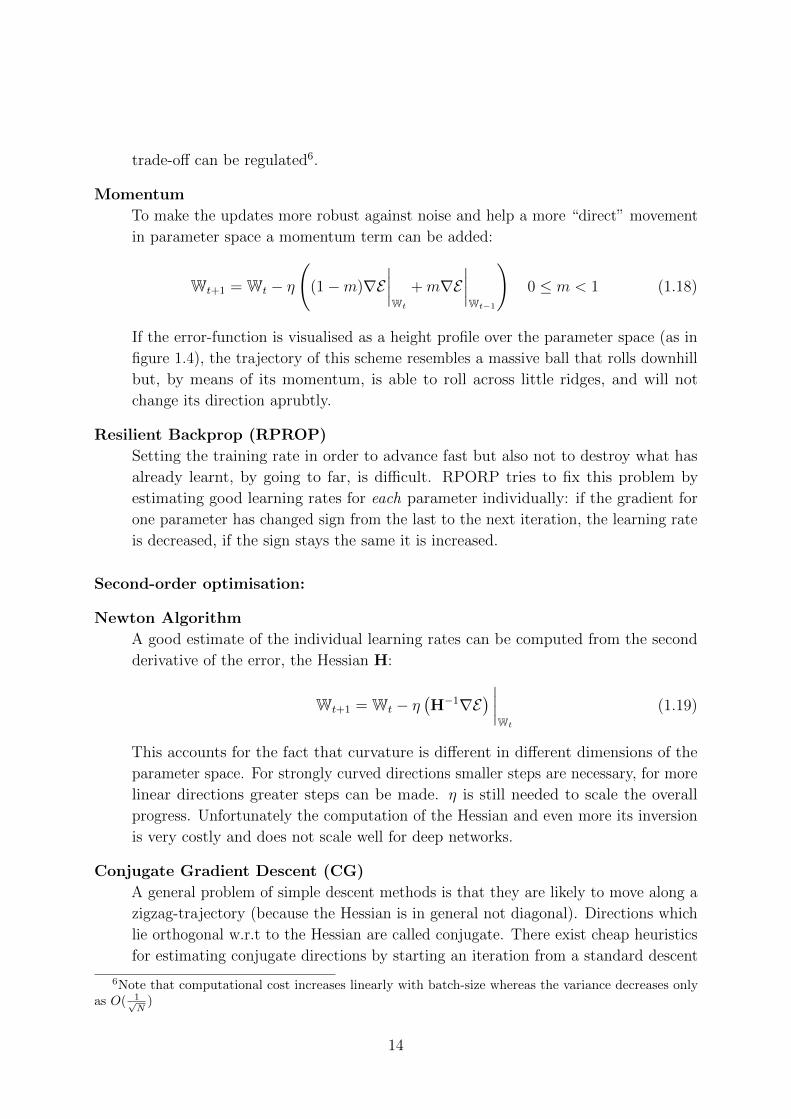
The first step is to imitate simple cells: in the hidden layer several filters or feature maps

exist. The neurons of a feature map correspond to an area in the domain of the input

image2. All of these neurons only receive input from a local field of view due to sparse

connectivity. The neurons’ weights represent a linear shift-invariant filter that is applied

to this field.

Calculating the weighted sum for all hidden neurons in a feature map is a discrete

convolution. In 1 dimension, for a filter size (receptive field) of 2k + 1 = s, the activation

in the filter map is given by:

yj = h(aj) = h(k∑

i=−k

xiwj−i) = h(x ∗w)j (2.1)

Likewise for 2 dimensions w is square matrix and a double-sum is needed for the convolution.

If the input comes from a 2-dimensional feature map of size s× s with l different feature

maps and the current layer exhibits m filters the weights of the convolution kernel are

given by a tensor with shape [m, l, s, s]. It is worth noting that, unlike for a normal layer,

the parameter number is not affected by the extent of the input at all. Moreover, the

convolution is an operation of less computational cost compared to the matrix multiplication

of a standard layer (provided the layer sizes are equal).

x0x1

x2x3

x4x5

x6x7

x8x9

x0x1

x2x3x4

x5x6x7

x8

Figure 2.1: The flat “non-spatial” input neuron vector is reshaped into a matrix so that eachneuron corresponds to a pixel in space. Within the neighbourhood of this pixel in the previouslayer (illustrated in green for neuron x7) the response of a filter (defined by connection weights) iscomputed. The response determines the neuron’s activation. As each neuron only has connectionswithin a local window and the pattern of connection weights is the same for all neurons, thiscomputation is equivalent to a convolution

The different feature maps can be imagined as a stack with a third dimension additional to

the two spatial dimensions. Likewise do the filter kernels have a third dimension because

2Due to border effects the valid image region has some offset from the edges.

18

they can combine all the feature maps in the previous layer - but the convolution is still

only across the two-dimensional domain.

As a consequence of weight sharing, all output neurons in a CNN process the input

data of their corresponding receptive fields in exactly the same way. Therefore such a

network can be viewed as many parallel networks with a single output neuron, glued next

to each other on a grid. The receptive fields are overlapping (as they are bigger than the

stride), hence creating one network is more efficient than many because the feature maps

can be reused within the implementation.

There exist some variations of usage of convolutions: for input images with several

channels (colour, depth etc.) the channels are processed like feature maps in the previous

layer. Convolution kernels can also be even-sized, in which case a neuron in the feature

map does not directly correspond to a pixel/neuron in the previous layer but “sits in

between”. Convolutions need not be dense, meaning that it is possible to leave out neurons

in the hidden layer, so that the receptive fields do not overlap; this is mainly done to

reduce computation. Input can have higher dimensions than two. Then the convolution is

required to be carried out across more dimensions, which increases computational cost.

2.2.2 Max-Pooling

The second step is inspired by the complex cells’ integration capability: if a filter detects

a feature, such as a line with certain angle, it is of greater importance what is detected

than where exactly it is. The fine spatial resolution of the filter maps is not needed and

processing can be made more sparse and computationally efficient by reducing it. This

also gives rise to translation invariance and slight rotational invariance. Note that this

invariance is not to be confused with the translation invariance resulting from convolution:

the latter ensures that the the same objects in an image will be detected the same way

regardless of their position. The invariance due to pooling makes the combination of

features invariant at the length scale of the pool size.

Plain sub-sampling is equivalent to a strided convolution. Alternatively the average

across a pool in the feature map can be used. Comparisons by [LeCun and Bengio, 1995]

have shown that taking the maximum of the pool outperforms taking the average and has

therefore become the standard.

2.3 Operation of a CNN

For illustration refer to figure 2.3. Several convolutional and pooling layers with a variable

number of filters and filter sizes are stacked together. In this part of the network the

19

x1

x2

x3

x4

x5

x6

x7

x8

x9

x10

y0

y1

y2

Input xConvolution

resultMaxpooling

result

Outputactiva-tion y

w ∈ R5

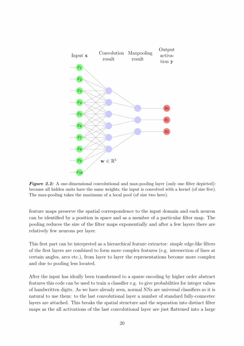
Figure 2.2: A one-dimensional convolutional and max-pooling layer (only one filter depicted):because all hidden units have the same weights, the input is convolved with a kernel (of size five).The max-pooling takes the maximum of a local pool (of size two here).

feature maps preserve the spatial correspondence to the input domain and each neuron

can be identified by a position in space and as a member of a particular filter map. The

pooling reduces the size of the filter maps exponentially and after a few layers there are

relatively few neurons per layer.

This first part can be interpreted as a hierarchical feature extractor: simple edge-like filters

of the first layers are combined to form more complex features (e.g. intersection of lines at

certain angles, arcs etc.), from layer to layer the representations become more complex

and due to pooling less located.

After the input has ideally been transformed to a sparse encoding by higher order abstract

features this code can be used to train a classifier e.g. to give probabilities for integer values

of handwritten digits. As we have already seen, normal NNs are universal classifiers so it is

natural to use them: to the last convolutional layer a number of standard fully-conncetec

layers are attached. This breaks the spatial structure and the separation into distinct filter

maps as the all activations of the last convolutional layer are just flattened into a large

20

Figure 2.3: Schematic visualisation of a CNN. The “stacks” in each layer illustrate a numberof feature maps. [source: http://deeplearning.net/tutorial/lenet.html]

vector.

The training procedure is in principle the same as for normal NNs. Like for normal

NNs the initialisation of the convolutional filters is usually random and for quite often

Gabor-like filters automatically evolve during optimisation. In other cases Gabor-Filters

can be used as initial values or filters that have separately been learnt e.g. by k-means or

PCA.

2.3.1 Providing traing data to a CNN for image-to-image tasks

Patch creation

Generally, feeding the whole image to a NN is computationally intractable with current

hardware, and it also creates problems for images of different sizes. Instead the image is

cut into smaller, square patches of constant size. Depending on the patch size, multiple

patches can be stacked to form a mini-batch which is used for Backprop-training. Using all

patches from all training images as in full-batch training is also computationally infeasible.

Many objects in images are invariant under congruence transformations i.e. transla-

tion, reflection and rotation. This can be exploited by augmenting the available data by

application of these transformations. When training the the cutting of patches is subject

to a random offsets in the whole image, thus yielding translated patches. Reflections were

applied by flipping axes of the images. This can be done in constant time by creating

strided memviews of the images. Rotations3 and other deformations are computationally

more intense and can be done in background processes.

3except by 90◦

21

Label creation

A CNN with no fully-connected layers at the end has multiple output neurons, correspond-

ing to a grid in image space. Due to the max-pooling, neurons in the output layer of a

deep CNN are separated by more than one pixel in the original image space. If neurons

are aligned so that they lie at the center pixel of their receptive fields, the pixel distance

of two output neurons is called stride; e.g. after three times max-pooling by a factor of

two the resulting stride is 23 = 8. The labels to which the output neurons are trained are

determined by sub-sampling the labels with the corresponding stride(see figure 2.4).

Independent of the pooling, the total receptive field is even bigger because the con-

volutional filters take into account neighbouring neurons/pixels in each layer, as a side

effect this causes a boundary region in the input domain for which no predictions can be

made4.

To obtain a dense prediction for each pixel in the image, not just a strided one, it

is necessary to feed the input patch several times through the network and shift it by one

pixel. A dense image is generate by combining predictions of the output neurons. As this

is computationally inefficient max-fragment-pooling (MFP) can be used which calculates

all possible shifts in one pass.

4To make a prediction there, a patch must be created s.t. this regions does not lie on the boundary.Alternatively good results can be achieved by mirroring the boundary.

22

Figure 2.4: CNN data for image-to-image tasks:top left Input image with border region indicated: due to convolution borders a stripe occursfor which no predictions are made.top right Image with true label overlaid. In green is the strided array of output neurons for aparticular CNN indicated.bottom left From the true labels, training labels were created for each neuron by subsamplingthe labels (For better visualisation the labels were scaled up to cover the whole block as opposedto only the center pixel)bottom right Strided predictive probability map from a trained NN. Each “block” correspondsto the output of one neuron at its center. (For better visualisation the predictions were scaledup to cover the whole block as opposed to only the center pixel).

.

23

List of Figures

1.1 A single neuron . . . . . . . . . . . . . . . . . . . . . . . . . . . . . . . . . 5

1.2 Simple 2-layer network . . . . . . . . . . . . . . . . . . . . . . . . . . . . . 7

1.3 Comparison of error-functions . . . . . . . . . . . . . . . . . . . . . . . . . 11

1.4 Gradient Descent . . . . . . . . . . . . . . . . . . . . . . . . . . . . . . . . 13

2.1 Reshaping networks from 1d to 2d . . . . . . . . . . . . . . . . . . . . . . . 18

2.2 Convolution and Max-Pooling Layer . . . . . . . . . . . . . . . . . . . . . 20

2.3 Convolutional Neural Network . . . . . . . . . . . . . . . . . . . . . . . . . 21

2.4 CNN data for image-to-image tasks . . . . . . . . . . . . . . . . . . . . . . 23

24

Bibliography

[Bishop et al., 2006] Bishop, C. M. et al. (2006). Pattern recognition and machine learning,

volume 1. springer New York.

[Cybenko, 1989] Cybenko, G. (1989). Approximation by superpositions of a sigmoidal

function. Mathematics of control, signals and systems, 2(4):303–314.

[Fukushima, 1980] Fukushima, K. (1980). Neocognitron: A self-organizing neural network

model for a mechanism of pattern recognition unaffected by shift in position. Biological

cybernetics, 36(4):193–202.

[Hodgkin and Huxley, 1952] Hodgkin, A. L. and Huxley, A. F. (1952). A quantitative

description of membrane current and its application to conduction and excitation in

nerve. The Journal of physiology, 117(4):500.

[Hubel and Wiesel, 1962] Hubel, D. H. and Wiesel, T. N. (1962). Receptive fields, binoc-

ular interaction and functional architecture in the cat’s visual cortex. The Journal of

physiology, 160(1):106.

[Lazar et al., 2009] Lazar, A., Pipa, G., and Triesch, J. (2009). Sorn: a self-organizing

recurrent neural network. Frontiers in computational neuroscience, 3.

[LeCun and Bengio, 1995] LeCun, Y. and Bengio, Y. (1995). Convolutional networks for

images, speech, and time series. The handbook of brain theory and neural networks,

3361.

[LeCun et al., 1998] LeCun, Y., Bottou, L., Bengio, Y., and Haffner, P. (1998). Gradient-

based learning applied to document recognition. Proceedings of the IEEE, 86(11):2278–

2324.

[LeCun et al., 2012] LeCun, Y. A., Bottou, L., Orr, G. B., and Muller, K.-R. (2012).

Efficient backprop. In Neural networks: Tricks of the trade, pages 9–48. Springer.

[McCulloch and Pitts, 1943] McCulloch, W. S. and Pitts, W. (1943). A logical calculus

of the ideas immanent in nervous activity. The bulletin of mathematical biophysics,

5(4):115–133.

25

[Rosenblatt, 1958] Rosenblatt, F. (1958). The perceptron: a probabilistic model for

information storage and organization in the brain. Psychological review, 65(6):386.

[Rumelhart et al., 1986] Rumelhart, D. E., Hinton, G. E., , and Williams, R. J. (1986).

Learning representations by back-propagating errors. Nature, 323:533–536.

[Young, 1938] Young, J. Z. (1938). The functioning of the giant nerve fibres of the squid.

Journal of Experimental Biology, 15(2):170–185.

26