METRIC SPACES

KEITH CONRAD

1. Introduction

As calculus developed, eventually turning into analysis, concepts first explored on thereal line (e.g., a limit of a sequence of real numbers) eventually extended to other spaces(e.g., a limit of a sequence of vectors or of functions), and in the early 20th century a generalsetting for analysis was formulated, called a metric space. It is a set on which a notion ofdistance between any two elements is defined, and in which notions from calculus in R (openand closed intervals, convergent sequences, continuous functions) can be studied. Many ofthe fundamental types of spaces used in analysis are metric spaces (e.g., Hilbert spaces andBanach spaces), so metric spaces are one of the first abstractions that has to be masteredin order to learn analysis.

2. Metric spaces

In R, the magnitude of a number x is its absolute value |x| and the distance betweentwo numbers x and y is the absolute value of their difference: |x− y|. In Rm, the length of

a vector x = (x1, . . . , xm) is its norm ||x|| =√x21 + · · ·+ x2m and the distance between two

vectors x = (x1, . . . , xm) and y = (y1, . . . , ym) is the norm of their difference: ||x − y|| =√(x1 − y1)2 + · · ·+ (xm − ym)2.The distance between points is essential in defining limits, the central idea of calculus.

There are limits of function values and limits of sequences. Focusing on the case of sequences(we will deal with limits and continuous functions in Section 8), we say a sequence {xn} ofreal numbers has limit x, and write limn→∞ xn = x or just xn → x, if for every ε > 0 thereis an N ≥ 1 (it is understood that N = Nε is an integer depending on ε) such that

n ≥ N =⇒ |xn − x| < ε.

For a sequence {xn} in Rm, we write limn→∞ xn = x or xn → x for an x ∈ Rm if for everyε > 0 there is an N = Nε such that

n ≥ N =⇒ ||xn − x|| < ε.

Distances are useful not only between points in Euclidean space, but also between func-tions. For continuous functions f, g : [0, 1]→ R, here are two different ways of defining howfar apart they are:

(2.1) max0≤x≤1

|f(x)− g(x)|,∫ 1

0|f(x)− g(x)| dx.

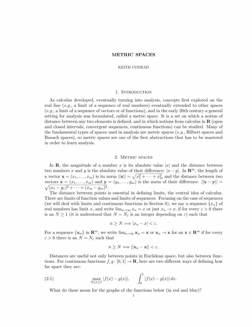
What do these mean for the graphs of the functions below (in red and blue)?1

2 KEITH CONRAD

0 1

The first formula in (2.1) is the length of the largest vertical line separating the graphs(the dashed line in the diagram), so saying f and g are close in this way means their graphsnever get far apart from each other. The second formula is the area of the region over [0, 1]that is enclosed by both graphs (“area between the curves”), so f and g are close in thisway if, roughly speaking, the graphs can only be far apart over small regions (thereby notaffecting the total area between the curves that much).

The desire to create a single framework for all the known settings where limit ideas areused inspired Maurice Frechet in his 1906 PhD thesis to make the following definition.

Definition 2.1. A metric on a set X is a function d : X ×X → R satisfying the followingthree properties:

(i) d(x, y) ≥ 0 for all x and y in X, with d(x, y) = 0 if and only if x = y,(ii) d(x, y) = d(y, x) for all x and y in X,

(iii) d(x, y) ≤ d(x, z) + d(z, y) for all x, y, z ∈ X.

A set X together with a choice of a metric d on it is called a metric space and is denoted(X, d), or just denoted X if the metric1 is understood from context.

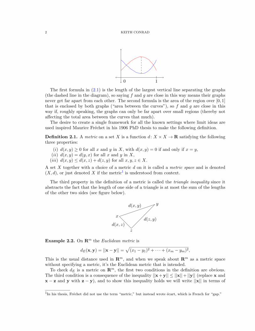
The third property in the definition of a metric is called the triangle inequality since itabstracts the fact that the length of one side of a triangle is at most the sum of the lengthsof the other two sides (see figure below).

x

y

z

d(x, y)

d(z, y)d(x, z)

Example 2.2. On Rm the Euclidean metric is

dE(x,y) = ||x− y|| =√

(x1 − y1)2 + · · ·+ (xm − ym)2,

This is the usual distance used in Rm, and when we speak about Rm as a metric spacewithout specifying a metric, it’s the Euclidean metric that is intended.

To check dE is a metric on Rm, the first two conditions in the definition are obvious.The third condition is a consequence of the inequality ||x + y|| ≤ ||x||+ ||y|| (replace x andx − z and y with z − y), and to show this inequality holds we will write ||x|| in terms of

1In his thesis, Frechet did not use the term “metric,” but instead wrote ecart, which is French for “gap.”

METRIC SPACES 3

the dot product: ||x||2 = x21 + · · ·+ x2m = x · x, so

||x + y||2 = (x + y) · (x + y)

= x · x + x · y + y · x + y · y= ||x||2 + 2x · y + ||y||2

≤ ||x||2 + 2|x · y|+ ||y||2.The famous Cauchy–Schwarz inequality says |x · y| ≤ ||x||||y||, so

||x + y||2 ≤ ||x||2 + 2||x||||y||+ ||y||2 = (||x||+ ||y||)2

and now take square roots.A different metric on Rm is

d∞(x,y) = max1≤i≤m

|xi − yi|.

Again, the first two conditions of being a metric are clear, and to check the triangle inequalitywe use the fact that it is known for the absolute value. If max |xi − yi| = |xk − yk| for aparticular k from 1 to m, then d∞(x,y) = |xk − yk|, so

d∞(x,y) ≤ |xk − zk|+ |zk − yk| ≤ max1≤i≤m

|xi − zi|+ max1≤i≤m

|zi − yi| = d∞(x, z) + d∞(z,x).

While the metrics dE and d∞ on Rm are different, they’re not that different from eachother since each is bounded by a constant multiple of the other one:

(2.2) dE(x,y) ≤√md∞(x,y), d∞(x,y) ≤ dE(x,y).

Example 2.3. Let C[0, 1] be the space of all continuous functions [0, 1]→ R. Two metricsused on C[0, 1] are in (2.1):

d∞(f, g) = max0≤x≤1

|f(x)− g(x)|, d1(f, g) =

∫ 1

0|f(x)− g(x)| dx.

Checking these are metrics is left to the reader.2 Notice for d1 that the condition d1(f, g) =

0 =⇒ f = g for being a metric uses continuity of the functions to know∫ 10 |f(x)−g(x)| dx =

0 =⇒ |f(x)− g(x)| = 0 for all x ∈ [0, 1].3

Unlike with the two metrics on Rm in Example 2.2, while we have d1(f, g) ≤ d∞(f, g)there is no constant A > 0 that makes d∞(f, g) ≤ Ad1(f, g) for all f and g. These metricsd1 and d∞ on C[0, 1] are quite different. In terminology we’ll meet later, C[0, 1] is completefor d∞ but not for d1.

Example 2.4. If (X, d) is a metric space and Y is any subset of X, then Y with themetric d|Y that is d with its domain restricted to Y ×Y is also a metric space (check!). Forexample, any subset of R is a metric space using d(x, y) = |x− y| for x and y in the subset.

Example 2.5. Every set X can be given the discrete metric

d(x, y) =

{0, if x = y,

1, if x 6= y,

2For d∞ to make sense requires each continuous function on [0, 1] to have a maximum value. This is theExtreme Value Theorem, which we’ll prove later as Theorem 8.2. It is convenient to have d∞ availablestrictly for examples before then.

3For p ≥ 1 the function dp(f, g) = p

√∫ 1

0|f(x)− g(x)|p dx is a metric on C[0, 1], and as p → ∞, dp(f, g) →

max0≤x≤1 |f(x)− g(x)|, which is why the metric d∞ has the notation it does.

4 KEITH CONRAD

which sets all pairs of (distinct) points in X at distance 1 from each other. All threeconditions for being a metric are easy to check.

Example 2.6. If d is a metric on X, then the functions d′(x, y) = min(d(x, y), 1) andd′′(x, y) = d(x, y)/(1 + d(x, y)) are also metrics on X. The only part that requires carefulchecking is the triangle inequality, which is left to the reader. Note d′ and d′′ are bothbounded: they never take a value larger than 1. These two metrics are similar to theoriginal metric d when d has value at most 1:

(2.3) d(x, y) ≤ 1 =⇒ d′(x, y) = d(x, y) and1

2d(x, y) ≤ d′′(x, y) ≤ d(x, y).

If d(x, y) > 1 then d′ and d′′ change the distance between x and y in different ways: d′

redefines the distance to be 1, while d′′ makes the distance less than 1 in a smoother way.

3. Limit of a sequence in a metric space

Armed with a notion of distance, as codified in a choice of a metric, we can carry overthe definition of the limit of a sequence from Euclidean space to metric spaces.

Definition 3.1. For a sequence xn in a metric space (X, d), we say xn converges to x ∈ X,and write limn→∞ xn = x or xn → x, if for every ε > 0 there is an N = Nε such that

n ≥ N =⇒ d(xn, x) < ε.

If a sequence in (X, d) has a limit we say the sequence is convergent.

Example 3.2. For x ∈ X, the constant sequence {x, x, x, . . .} is convergent with limit x.Similarly, any eventually constant sequence (xn = x for all large n) is convergent. This istrue no matter what metric is used.

Example 3.3. If d is the discrete metric on X then a convergent sequence must be even-tually constant: if d(xn, x) < 1 for large n then xn = x for large n.

These examples are boring. The reader should know many interesting examples of con-vergent sequences in R from calculus.

Saying xn → x in a metric space (X, d) is the same as saying d(xn, x) → 0 in R:convergence of a sequence to a specific value means the distance between the terms of thesequence and that value tends to 0.

To get used to the terminology, let’s prove four intuitively reasonable theorems aboutconvergent sequences (try drawing a picture for each one).

Theorem 3.4. If a sequence {xn} in a metric space (X, d) converges then d(xn, xn+1)→ 0.

Proof. Showing the numbers d(xn, xn+1) tend to 0 means we want to show for every ε >0 that there is an N such that n ≥ N =⇒ d(xn, xn+1) < ε. (We don’t need to say|d(xn, xn+1)| < ε since values of a metric are nonnegative.)

Say limn→∞ xn = x. Using the triangle inequality,

d(xn, xn+1) ≤ d(xn, x) + d(x, xn+1) = d(xn, x) + d(xn+1, x).

The two terms on the right get small when n is large, so d(xn, xn+1) gets small when n islarge. To be precise, for ε > 0 also ε/2 > 0, so there’s an N ≥ 1 such that for all m ≥ Nwe have d(xm, x) < ε/2. Therefore

n ≥ N =⇒ n+ 1 ≥ N =⇒ d(xn, xn+1) ≤ d(xn, x) + d(xn+1, x) <ε

2+ε

2= ε.

�

METRIC SPACES 5

Remark 3.5. If we had stuck with ε rather than ε/2 all the way through the proof thenwe’d get 2ε at the end instead of ε, and then we’d have to say “Now go back and replace εwith ε/2 . . .” to get the desired conclusion. The idea of using ε/2 in place of ε in the middlein order to get a single ε at the end is called an ε/2 argument. This type of reasoning occursall the time in analysis. Instead of ε/2 one might use ε/3,

√ε, or ε/2n (the last one is good

if we have a whole sequence of terms that need bounds whose sum is still less than ε).

Theorem 3.6. Every subsequence of a convergent sequence in a metric space is also con-vergent, with the same limit.

Proof. Let xn → x in (X, d) and let {xni} be a subsequence of {xn}. Then n1 < n2 < · · · .Set yi = xni . We want to show yi → x.

For ε > 0 there is an N such that n ≥ N =⇒ d(xn, x) < ε. Since the integers ni areincreasing, we have ni ≥ N if we go out far enough: there’s an I such that i ≥ I =⇒ ni ≥N =⇒ d(xni , x) < ε, so d(yi, x) < ε. Thus yi → x. �

Theorem 3.7. In a metric space (X, d), if two sequences {xn} and {x′n} converge to thesame value then d(xn, x

′n)→ 0.

Proof. Suppose xn → x and x′n → x. Then d(xn, x′n) ≤ d(xn, x) + d(x, x′n) = d(xn, x) +

d(x′n, x) and the last two terms get small for large n. This suggests using an ε/2 argument.For each ε > 0 there’s an N1 such that n ≥ N1 =⇒ d(xn, x) < ε/2 and an N2 such that

n ≥ N2 =⇒ d(x′n, x) < ε/2. Set N = max(N1, N2), so

n ≥ N =⇒ d(xn, x′n) ≤ d(xn, x) + d(x′n, x) <

ε

2+ε

2= ε.

�

The converse to Theorem 3.7 is false: sequences for which d(xn, x′n) → 0 do not have

to converge. After all, let {xn} be an arbitrary sequence and let x′n = xn for all n, sod(xn, x

′n) = 0 all the time.

The next result is a partial converse to Theorem 3.7.

Theorem 3.8. In a metric space (X, d), if xn → x and {x′n} is a sequence such thatd(xn, x

′n)→ 0 then x′n → x.

Proof. This will be an ε/2 argument.Pick ε > 0. We want to find an N such that n ≥ N =⇒ d(x′n, x) < ε.There’s an N1 such that n ≥ N1 =⇒ d(xn, x) < ε/2. Since the real numbers d(xn, x

′n)

tend to 0, there’s an N2 such that n ≥ N2 =⇒ d(xn, x′n) < ε/2. Setting N = max(N1, N2),

we have

n ≥ N =⇒ d(x′n, x) ≤ d(x′n, xn) + d(xn, x) <ε

2+ε

2= ε.

�

Example 3.9. On Rm, because the metrics dE and d∞ are each bounded above by aconstant multiple of the other (see (2.2)), we have dE(xn,x)→ 0 if and only if d∞(xn,x)→0. Therefore convergence of sequences in Rm for both metrics means the same thing (withthe same limits).

Example 3.10. In Example 2.6 we introduced two alternatives to a metric d that are bothbounded metrics: d′(x, y) = min(d(x, y), 1) and d′′(x, y) = d(x, y)/(1 + d(x, y)). Condition(2.3) shows d′ and d′′ have the same convergent sequences and limits as d.

6 KEITH CONRAD

Example 3.11. In C[0, 1] consider the sequence of functions xn for n ≥ 1, graphed below.

0 1

This sequence converges to 0 in the metric d1 but not in the metric d∞:

d1(xn, 0) =

∫ 1

0|xn| dx =

1

n+ 1→ 0, d∞(xn, 0) = max

0≤x≤1|xn| = 1.

In fact the sequence {xn} in C[0, 1] has no limit at all relative to the metric d∞.To prove {xn} has no limit in (C[0, 1], d∞), not just that the constant function 0 is not

a limit, we seek a property that all convergent sequences satisfy and the sequence {xn} in(C[0, 1], d∞) does not satisfy. Theorem 3.4 tells us every convergent sequence in a metricspace has the distance between consecutive terms tending to 0. Might d∞(xn, xn+1) nottend to 0? Well,

d∞(xn, xn+1) = max0≤x≤1

|xn − xn+1| = max0≤x≤1

(xn − xn+1)

and by calculus xn−xn+1 = xn(1−x) is is maximized on [0, 1] at x = n/(n+ 1), where thevalue is (n/(n+ 1))n(1− n/(n+ 1)) ∼ (1/e)(1/(n+ 1))→ 0. Our idea failed to help.

Rather than looking at the distance between consecutive terms in a sequence, we can lookat the distance between the nth and (2n)th terms. In the proof of Theorem 3.4 it wasn’t socrucial that the terms from the sequence were consecutive. The exact same reasoning usedthere works with the nth and (2n)th terms, so if the sequence {xn} in (C[0, 1], d∞) has alimit then d∞(xn, x2n)→ 0 as n→∞. Since

d∞(xn, x2n) = max0≤x≤1

|xn − x2n| = max0≤x≤1

xn(1− xn)

and the function xn(1−xn) on [0, 1] has its maximum value at x = 1/ n√

2, where xn(1−xn) =(1/2)(1/2) = 1/4, which is independent of n, this proves {xn} has no limit in (C[0, 1], d∞).

To know what a metric on a set X means, know what it means to say two points areclose in that metric. For example, when we say fn → f in (C[0, 1], d∞), it means the graphof fn is getting close to f uniformly (at the same rate) over all of [0, 1] as n→∞. A pictureof f (in blue) and an approximation fn (in red) in the metric d∞ is pictured below.

0 1

y = f(x)

y = fn(x)

METRIC SPACES 7

When fn → f in (C[0, 1], d∞) we say fn → f uniformly on [0, 1]. This implies pointwiseconvergence: fn(a)→ f(a) for each a ∈ [0, 1] since

|fn(a)− f(a)| ≤ max0≤x≤1

|fn(x)− f(x)| = d∞(fn, f)→ 0.

However the converse is false: if fn(a) → f(a) for each a ∈ [0, 1] it does not meand∞(fn, f) → 0. Pointwise convergence does not imply convergence can be controlled inthe same way simultaneously on the whole domain [0, 1]. Consider the functions fn(x) on[0, 1] graphed below which are an isoceles triangle of height 1 over [0, 1/n] and 0 for x ≥ 1/n.We have fn(0) = 0 for all n, and for each a ∈ (0, 1] we have fn(a) = 0 for large enough n,so fn(a)→ 0 for each a ∈ [0, 1], but d∞(fn, 0) = 1 so fn does not get close to the function0 as n gets large because every fn has a peak of height 1.

0 11/n

1

y = fn(x)

Changing metrics from d∞ to d1, saying fn → f in (C[0, 1], d1) does not guaranteepointwise convergence. For example, d1(x

n, 0) → 0 and numerically an → 0 for 0 ≤ a < 1,but not at a = 1.

4. Cauchy sequences and completeness

One aspect of infinite series that many students find hard to understand is how conver-gence tests really work: one may prove with the comparison test that

∑k≥1 x

k/k2 converges

for x in the interval [−1, 1], but what does it converge to? The subtlety here is that we aresaying something converges without identifying the limit in any concrete way. (Saying “theseries is what the limit is” sounds more circular than explanatory.) Often we want to provea sequence (of numbers or functions or shapes) has a limit even if we don’t yet have a tidyname for the limiting object. How can convergence be detected before the limit is known?

A clue is in Theorem 3.4: if xn → x in a metric space (X, d) then d(xn, xn+1)→ 0. Theconclusion makes no reference to the original limit x. Unfortunately, this property thatthe terms become “consecutively close” is not good enough to characterize convergence ingeneral metric spaces. We saw this in Example 3.11, where the sequence of power functionsxn in (C[0, 1], d∞) does not converge but d∞(xn, xn+1) ∼ (1/e)(1/(n+1))→ 0. A more basicexample is the harmonic series, which diverges and its partial sums Hn = 1+1/2+ · · ·+1/nare consecutively close: |Hn −Hn+1| = 1/(n+ 1)→ 0.

By making a slight change in the proof of Theorem 3.4, we get a much stronger conclusionthan consecutive closeness, and this stronger conclusion will be exactly what we need.

Theorem 4.1. If {xn} is a convergent sequence in a metric space (X, d) then the termsof the sequence become “uniformly close”: for every ε > 0 there is an N ≥ 1 such thatm,n ≥ N =⇒ d(xm, xn) < ε.

8 KEITH CONRAD

Proof. We run through the proof of Theorem 3.4 and make a few changes. Letting x =limn→∞ xn, the triangle inequality tells us for all m and n that

d(xm, xn) ≤ d(xm, x) + d(x, xn) = d(xm, x) + d(xn, x).

We now make an ε/2 argument. For every ε > 0 there’s an N ≥ 1 such that for all n ≥ Nwe have d(xn, x) < ε/2. Therefore

m,n ≥ N =⇒ d(xm, xn) ≤ d(xm, x) + d(xn, x) <ε

2+ε

2= ε.

�

This concept of uniform closeness, which is a property of a sequence involving no directreference to a hypothetical limit, is much more stringent than consecutive closeness. Forexample, if Hn = 1 + 1/2 + · · · + 1/n then the numbers Hn are consecutively close (thatis, |Hn −Hn+1| → 0) but they are not uniformly close. It can be shown, for instance, that|Hn −H2n| → log 2 ≈ .693.

When calculus was acquiring rigorous foundations in the 19th century, it was realized thatuniform closeness in Theorem 4.1 captures the idea of convergence for sequences withoutmentioning a limit for the sequence. This property is not actually called uniform closeness,but is named in honor of Cauchy, who articulated and used it in the setting of infinite series.

Definition 4.2. A sequence {xn} in a metric space (X, d) is called a Cauchy sequence iffor every ε > 0 there is an N = Nε such that for all m,n ≥ N we have d(xm, xn) < ε.

Theorem 4.3. Every convergent sequence in a metric space is a Cauchy sequence.

Proof. This is Theorem 4.1. �

Corollary 4.4. If (X, d) is a metric space and Y is a subset of X given the induced metricd|Y , then any sequence in Y that converges in X is a Cauchy sequence in (Y, d|Y ).

Proof. A sequence {yn} in Y that converges in X is Cauchy in X by Theorem 4.3. Sincethe metric d on X is the metric we are using on Y , the Cauchy property of {yn} in X canbe viewed as the Cauchy property in Y . �

Example 4.5. Consider the interval (0,∞) as a metric space using the absolute valuemetric induced from R. We have 1/n → 0 in R, but the sequence {1/n} has no limit in(0,∞) since 0 6∈ (0,∞). The sequence {1/n} is a Cauchy sequence in (0,∞) by Corollary4.4 but it is not a convergent sequence in (0,∞).

Example 4.6. On Rm, the metrics dE and d∞ satisfy d∞ ≤ dE ≤√md∞, so a sequence

in Rm is Cauchy with respect to one of these metrics if and only if it is Cauchy with respectto the other one.

Being a Cauchy sequence means if you go out far enough into the sequence then all theterms from some point onwards are as close together as you wish. While this propertyis much stronger than being a consecutively close sequence, a sequence whose terms getconsecutively close rapidly enough is a Cauchy sequence. The next theorem says that beingconsecutively close at least at the rate of a geometric progression is rapid enough.

Theorem 4.7. If {xn} is a sequence in a metric space (X, d) such that d(xn, xn+1) ≤ arnfor all n, where a > 0 and 0 < r < 1, then {xn} is a Cauchy sequence.

METRIC SPACES 9

Proof. For 1 ≤ m < n, a massive use of the triangle inequality tells us

d(xm, xn) ≤ d(xm, xm+1) + d(xm+1, xm+2) + · · ·+ d(xn−1, xn)

≤ arm + arm+1 + · · ·+ arn−1

<

∞∑k=m

ark

=arm

1− r.

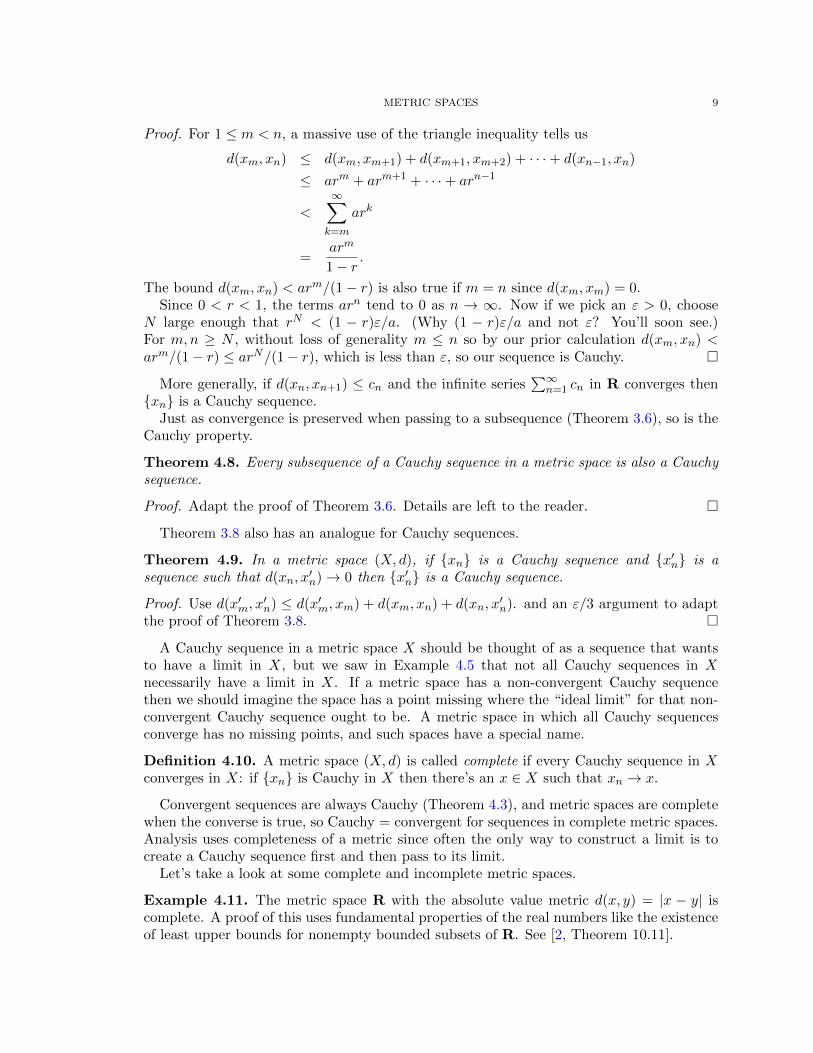
The bound d(xm, xn) < arm/(1− r) is also true if m = n since d(xm, xm) = 0.Since 0 < r < 1, the terms arn tend to 0 as n → ∞. Now if we pick an ε > 0, choose

N large enough that rN < (1 − r)ε/a. (Why (1 − r)ε/a and not ε? You’ll soon see.)For m,n ≥ N , without loss of generality m ≤ n so by our prior calculation d(xm, xn) <arm/(1− r) ≤ arN/(1− r), which is less than ε, so our sequence is Cauchy. �

More generally, if d(xn, xn+1) ≤ cn and the infinite series∑∞

n=1 cn in R converges then{xn} is a Cauchy sequence.

Just as convergence is preserved when passing to a subsequence (Theorem 3.6), so is theCauchy property.

Theorem 4.8. Every subsequence of a Cauchy sequence in a metric space is also a Cauchysequence.

Proof. Adapt the proof of Theorem 3.6. Details are left to the reader. �

Theorem 3.8 also has an analogue for Cauchy sequences.

Theorem 4.9. In a metric space (X, d), if {xn} is a Cauchy sequence and {x′n} is asequence such that d(xn, x

′n)→ 0 then {x′n} is a Cauchy sequence.

Proof. Use d(x′m, x′n) ≤ d(x′m, xm) + d(xm, xn) + d(xn, x

′n). and an ε/3 argument to adapt

the proof of Theorem 3.8. �

A Cauchy sequence in a metric space X should be thought of as a sequence that wantsto have a limit in X, but we saw in Example 4.5 that not all Cauchy sequences in Xnecessarily have a limit in X. If a metric space has a non-convergent Cauchy sequencethen we should imagine the space has a point missing where the “ideal limit” for that non-convergent Cauchy sequence ought to be. A metric space in which all Cauchy sequencesconverge has no missing points, and such spaces have a special name.

Definition 4.10. A metric space (X, d) is called complete if every Cauchy sequence in Xconverges in X: if {xn} is Cauchy in X then there’s an x ∈ X such that xn → x.

Convergent sequences are always Cauchy (Theorem 4.3), and metric spaces are completewhen the converse is true, so Cauchy = convergent for sequences in complete metric spaces.Analysis uses completeness of a metric since often the only way to construct a limit is tocreate a Cauchy sequence first and then pass to its limit.

Let’s take a look at some complete and incomplete metric spaces.

Example 4.11. The metric space R with the absolute value metric d(x, y) = |x − y| iscomplete. A proof of this uses fundamental properties of the real numbers like the existenceof least upper bounds for nonempty bounded subsets of R. See [2, Theorem 10.11].

10 KEITH CONRAD

Example 4.12. The closed intervals [0, 1] and [0,∞) with metric from R are complete.The open intervals (0, 1) and (0,∞) with metric from R are not complete: a sequence inthe interval that tends to 0 is Cauchy but does not converge in the interval.

Example 4.13. The rational numbers Q with the absolute value metric d(r, s) = |r − s|are not complete. To prove this, pick an irrational real number L (like

√2 or π) and let

rn be the sequence of decimal approximations to L truncated at the 1/10n place. Eachfinite decimal is rational, so rn ∈ Q. Since rn → L in R, {rn} is a Cauchy sequence in Q(Corollary 4.4). However, {rn} has no limit in Q, so Q is not complete.

Example 4.14. The integers with the absolute value metric are complete: any Cauchysequence in Z (as a metric space inside R) is eventually constant. This is boring.

Example 4.15. A set X with the discrete metric on it (Example 2.5) is complete: if dis the discrete metric and d(xm, xn) < 1 then xm = xn, so every Cauchy sequence for thediscrete metric is an eventually constant sequence, which clearly converges.

Example 4.16. The metric space (C[0, 1], d∞) is complete. A proof is in Appendix A.

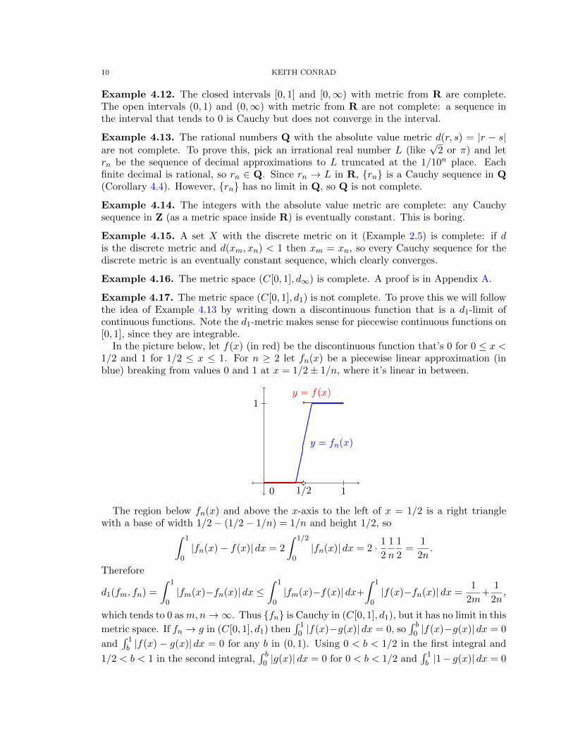
Example 4.17. The metric space (C[0, 1], d1) is not complete. To prove this we will followthe idea of Example 4.13 by writing down a discontinuous function that is a d1-limit ofcontinuous functions. Note the d1-metric makes sense for piecewise continuous functions on[0, 1], since they are integrable.

In the picture below, let f(x) (in red) be the discontinuous function that’s 0 for 0 ≤ x <1/2 and 1 for 1/2 ≤ x ≤ 1. For n ≥ 2 let fn(x) be a piecewise linear approximation (inblue) breaking from values 0 and 1 at x = 1/2± 1/n, where it’s linear in between.

y = fn(x)

y = f(x)

0 11/2

1

The region below fn(x) and above the x-axis to the left of x = 1/2 is a right trianglewith a base of width 1/2− (1/2− 1/n) = 1/n and height 1/2, so∫ 1

0|fn(x)− f(x)| dx = 2

∫ 1/2

0|fn(x)| dx = 2 · 1

2

1

n

1

2=

1

2n.

Therefore

d1(fm, fn) =

∫ 1

0|fm(x)−fn(x)| dx ≤

∫ 1

0|fm(x)−f(x)| dx+

∫ 1

0|f(x)−fn(x)| dx =

1

2m+

1

2n,

which tends to 0 asm,n→∞. Thus {fn} is Cauchy in (C[0, 1], d1), but it has no limit in this

metric space. If fn → g in (C[0, 1], d1) then∫ 10 |f(x)−g(x)| dx = 0, so

∫ b0 |f(x)−g(x)| dx = 0

and∫ 1b |f(x) − g(x)| dx = 0 for any b in (0, 1). Using 0 < b < 1/2 in the first integral and

1/2 < b < 1 in the second integral,∫ b0 |g(x)| dx = 0 for 0 < b < 1/2 and

∫ 1b |1− g(x)| dx = 0

METRIC SPACES 11

for 1/2 < b < 1. Therefore g(x) = 0 for 0 ≤ x < 1/2 and g(x) = 1 for 1/2 < x ≤ 1, but novalue can be assigned to g(1/2) to make this continuous.

When a metric space is not complete, like (Q, | · |) or (C[0, 1], d1), we want to “fill in allthe holes” to create a complete metric space containing the original one. To describe thislarger space, we need one more concept.

Definition 4.18. A subset S ⊂ X is called dense if every element of X is the limit of asequence in S or equivalently every open ball around an element of X contains an elementof S.

Example 4.19. The rational numbers are dense in R but the integers are not dense in R.

Definition 4.20. A completion of a metric space (X, d) is a complete metric space (X, d)

that contains X, the metric d restricted to X is d, and X is a dense subset of X.

Example 4.21. The completion of (Q, | · |) is (R, | · |). If we think of R inside R2 asthe x-axis then the completion of Q is not R2 even though R2 is complete because Q isnot dense in R2. The idea of a completion is filling in the holes (missing limits of Cauchysequences) and not adding anything more, which is why the completion of a metric spaceis required to have the original space as a dense subset.

Theorem 4.22. Every metric space has a completion.

Proof. See Appendix A. �

5. Open and closed subsets

In calculus, a lot of attention is paid to intervals: open intervals (a, b), closed intervals[a, b], and half-open intervals (a, b] and [a, b). Allowing the endpoints to be ±∞ introducesthe distinction between bounded and unbounded intervals. There are theorems about con-tinuous or differentiable functions on intervals (Intermediate Value Theorem, Extreme ValueTheorem, Mean Value Theorem), definite integrals are defined on intervals, and the set ofnumbers where a power series converges is an interval. What is so special about intervals?

It turns out that the key feature of intervals for one application may be quite differentfrom the key feature needed for another application. Over the next few sections we willisolate several of these features and present the generalization of each one in metric spaces.This leads to many special types of subsets of a metric space, such as open balls, closedballs, compact subsets, and connected subsets. We will see that

• open intervals (a, b) with a, b ∈ R generalize to open balls and connected subsets,• closed intervals [a, b] with a, b ∈ R will generalize to closed balls, compact subsets,

and connected subsets.

In this section we generalize open and closed intervals in R to open and closed balls of ametric space. Throughout, (X, d) is a metric space.

Definition 5.1. For a ∈ X and r ≥ 0, the open ball with center a and radius r is

B(a, r) = {x ∈ X : d(a, x) < r}

and the closed ball with center a and radius r is

B(a, r) = {x ∈ X : d(a, x) ≤ r}.

12 KEITH CONRAD

When r = 0, B(a, 0) = ∅ and B(a, 0) = {a} by the axioms for a metric. Some writersonly consider balls to have positive radius.

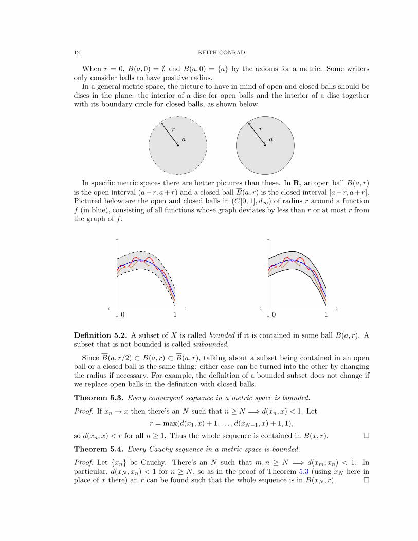
In a general metric space, the picture to have in mind of open and closed balls should bediscs in the plane: the interior of a disc for open balls and the interior of a disc togetherwith its boundary circle for closed balls, as shown below.

a

r

a

r

In specific metric spaces there are better pictures than these. In R, an open ball B(a, r)is the open interval (a− r, a+ r) and a closed ball B(a, r) is the closed interval [a− r, a+ r].Pictured below are the open and closed balls in (C[0, 1], d∞) of radius r around a functionf (in blue), consisting of all functions whose graph deviates by less than r or at most r fromthe graph of f .

0 1 0 1

Definition 5.2. A subset of X is called bounded if it is contained in some ball B(a, r). Asubset that is not bounded is called unbounded.

Since B(a, r/2) ⊂ B(a, r) ⊂ B(a, r), talking about a subset being contained in an openball or a closed ball is the same thing: either case can be turned into the other by changingthe radius if necessary. For example, the definition of a bounded subset does not change ifwe replace open balls in the definition with closed balls.

Theorem 5.3. Every convergent sequence in a metric space is bounded.

Proof. If xn → x then there’s an N such that n ≥ N =⇒ d(xn, x) < 1. Let

r = max(d(x1, x) + 1, . . . , d(xN−1, x) + 1, 1),

so d(xn, x) < r for all n ≥ 1. Thus the whole sequence is contained in B(x, r). �

Theorem 5.4. Every Cauchy sequence in a metric space is bounded.

Proof. Let {xn} be Cauchy. There’s an N such that m,n ≥ N =⇒ d(xm, xn) < 1. Inparticular, d(xN , xn) < 1 for n ≥ N , so as in the proof of Theorem 5.3 (using xN here inplace of x there) an r can be found such that the whole sequence is in B(xN , r). �

METRIC SPACES 13

Since convergent sequences are Cauchy, Theorem 5.3 is a special case of Theorem 5.4.

Definition 5.5. A subset U ⊂ X is called open if for each x ∈ U there’s an r > 0 such thatB(x, r) ⊂ U . We also consider the empty subset of X to be an open subset.

The idea behind the concept of a subset U being open is that the points in it are stableunder small perturbations: if we wiggle each element of U a little bit “in all directions”then we stay inside of U . Exactly how much we can wiggle without leaving U depends onhow close we are to the “edge” of U .

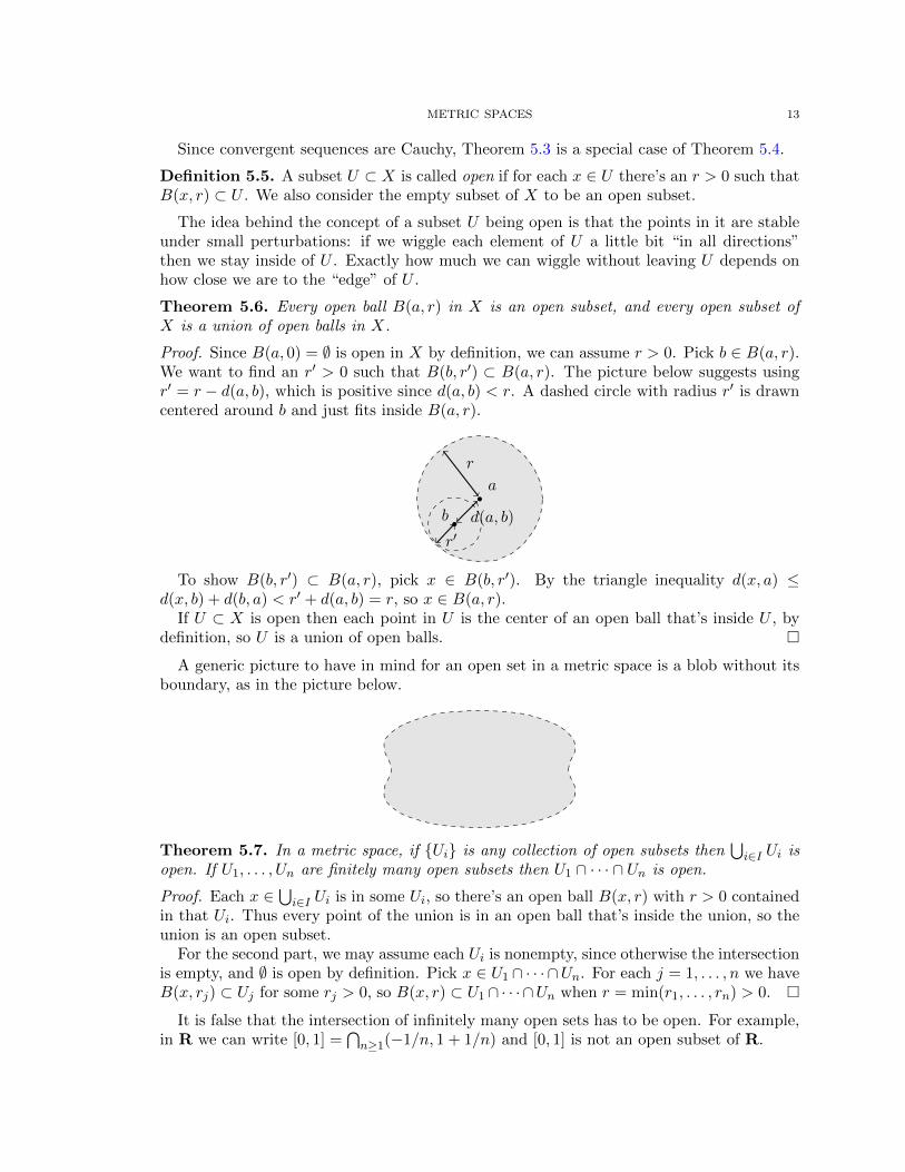
Theorem 5.6. Every open ball B(a, r) in X is an open subset, and every open subset ofX is a union of open balls in X.

Proof. Since B(a, 0) = ∅ is open in X by definition, we can assume r > 0. Pick b ∈ B(a, r).We want to find an r′ > 0 such that B(b, r′) ⊂ B(a, r). The picture below suggests usingr′ = r − d(a, b), which is positive since d(a, b) < r. A dashed circle with radius r′ is drawncentered around b and just fits inside B(a, r).

a

b

r

d(a, b)

r′

To show B(b, r′) ⊂ B(a, r), pick x ∈ B(b, r′). By the triangle inequality d(x, a) ≤d(x, b) + d(b, a) < r′ + d(a, b) = r, so x ∈ B(a, r).

If U ⊂ X is open then each point in U is the center of an open ball that’s inside U , bydefinition, so U is a union of open balls. �

A generic picture to have in mind for an open set in a metric space is a blob without itsboundary, as in the picture below.

Theorem 5.7. In a metric space, if {Ui} is any collection of open subsets then⋃

i∈I Ui isopen. If U1, . . . , Un are finitely many open subsets then U1 ∩ · · · ∩ Un is open.

Proof. Each x ∈⋃

i∈I Ui is in some Ui, so there’s an open ball B(x, r) with r > 0 containedin that Ui. Thus every point of the union is in an open ball that’s inside the union, so theunion is an open subset.

For the second part, we may assume each Ui is nonempty, since otherwise the intersectionis empty, and ∅ is open by definition. Pick x ∈ U1 ∩ · · · ∩Un. For each j = 1, . . . , n we haveB(x, rj) ⊂ Uj for some rj > 0, so B(x, r) ⊂ U1 ∩ · · · ∩Un when r = min(r1, . . . , rn) > 0. �

It is false that the intersection of infinitely many open sets has to be open. For example,in R we can write [0, 1] =

⋂n≥1(−1/n, 1 + 1/n) and [0, 1] is not an open subset of R.

14 KEITH CONRAD

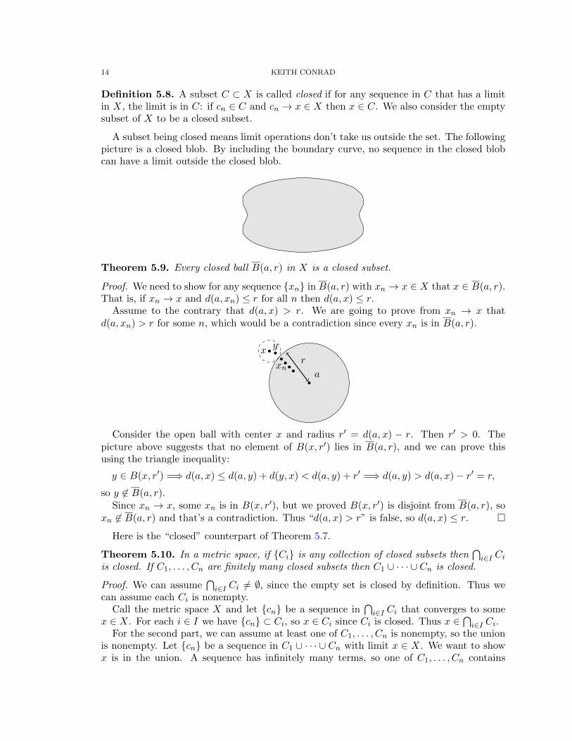
Definition 5.8. A subset C ⊂ X is called closed if for any sequence in C that has a limitin X, the limit is in C: if cn ∈ C and cn → x ∈ X then x ∈ C. We also consider the emptysubset of X to be a closed subset.

A subset being closed means limit operations don’t take us outside the set. The followingpicture is a closed blob. By including the boundary curve, no sequence in the closed blobcan have a limit outside the closed blob.

Theorem 5.9. Every closed ball B(a, r) in X is a closed subset.

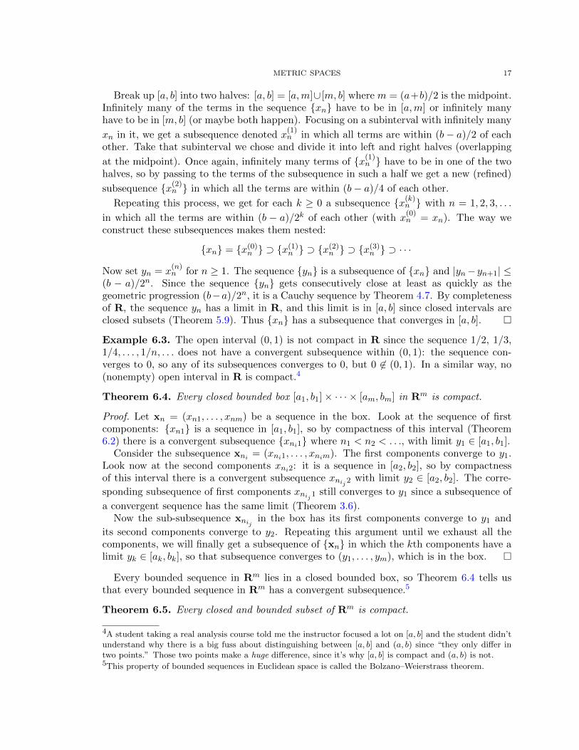
Proof. We need to show for any sequence {xn} in B(a, r) with xn → x ∈ X that x ∈ B(a, r).That is, if xn → x and d(a, xn) ≤ r for all n then d(a, x) ≤ r.

Assume to the contrary that d(a, x) > r. We are going to prove from xn → x thatd(a, xn) > r for some n, which would be a contradiction since every xn is in B(a, r).

a

rx y

xn

Consider the open ball with center x and radius r′ = d(a, x) − r. Then r′ > 0. Thepicture above suggests that no element of B(x, r′) lies in B(a, r), and we can prove thisusing the triangle inequality:

y ∈ B(x, r′) =⇒ d(a, x) ≤ d(a, y) + d(y, x) < d(a, y) + r′ =⇒ d(a, y) > d(a, x)− r′ = r,

so y 6∈ B(a, r).Since xn → x, some xn is in B(x, r′), but we proved B(x, r′) is disjoint from B(a, r), so

xn 6∈ B(a, r) and that’s a contradiction. Thus “d(a, x) > r” is false, so d(a, x) ≤ r. �

Here is the “closed” counterpart of Theorem 5.7.

Theorem 5.10. In a metric space, if {Ci} is any collection of closed subsets then⋂

i∈I Ci

is closed. If C1, . . . , Cn are finitely many closed subsets then C1 ∪ · · · ∪ Cn is closed.

Proof. We can assume⋂

i∈I Ci 6= ∅, since the empty set is closed by definition. Thus wecan assume each Ci is nonempty.

Call the metric space X and let {cn} be a sequence in⋂

i∈I Ci that converges to somex ∈ X. For each i ∈ I we have {cn} ⊂ Ci, so x ∈ Ci since Ci is closed. Thus x ∈

⋂i∈I Ci.

For the second part, we can assume at least one of C1, . . . , Cn is nonempty, so the unionis nonempty. Let {cn} be a sequence in C1 ∪ · · · ∪ Cn with limit x ∈ X. We want to showx is in the union. A sequence has infinitely many terms, so one of C1, . . . , Cn contains

METRIC SPACES 15

infinitely many terms of the sequence. That is, a subsequence of {cn} lies entirely insidesome Cj . Since any subsequence of a convergent sequence also converges with the samelimit (Theorem 3.6), and Cj is closed, it follows that x ∈ Cj ⊂ C1 ∪ · · · ∪ Cn. �

It is false that the union of infinitely many closed subsets has to be closed. For example,in R we can write (0, 1) =

⋃n≥1[1/n, 1− 1/n] and (0, 1) is not a closed subset of R.

Theorem 5.11. Every closed subset of a complete metric space is complete.

Proof. Let C be a closed subset of X. Any Cauchy sequence in C is Cauchy in X, so it hasa limit x ∈ X by completeness of X. Since C is a closed subset of X, we must have x ∈ C.Thus all Cauchy sequences in C converge in C, so C is complete. �

Definition 5.12. A limit point of a subset S ⊂ X is a point of X that is the limit of somesequence in S.

Definition 5.13. The closure of a subset S ⊂ X is the union of S and its limit points inX. This set is denoted S.

Example 5.14. For all a ∈ Rm and r > 0, B(a, r) = B(a, r): the closure of every(nonemtpy) open ball in Rm is the closed ball with the same center and radius. In generalmetric spaces, this intuitively appealing property might be false.

Theorem 5.15. For any subset S ⊂ X, its closure S is closed in X and S is the smallestclosed subset of X containing S. In particular, S is closed if and only if S = S.

Proof. If S ⊂ C ⊂ X and C is closed in X then any limit point of S lies in C, so S ⊂ C. Itremains to show S is closed.

Let {xn} be a sequence in S with limit x ∈ X. Since each xn is a limit point of S, there’ssome sn ∈ S such that d(xn, sn) < 1/n. Then xn → x and d(xn, sn) → 0, so sn → x byTheorem 3.8. Therefore x ∈ S. �

Dense subsets were defined in Definition 4.18. They can also be described using closures.

Theorem 5.16. A subset S ⊂ X is dense if and only if S = X.

Proof. Saying S is dense means every element of X is a limit point of S, so X ⊂ S. Thereverse containment is true by definition. �

We have developed properties of open subsets and closed subsets separately. The followingtheorem shows they are in fact complementary concepts!

Theorem 5.17. A subset of X is open if and only if its complement is closed.

Proof. Pick an open subset U . To prove its complement X − U is closed, we can assumeX − U 6= ∅ since the empty set is closed by definition.

Let {xn} be a sequence in X − U with limit x ∈ X. To prove x ∈ X − U , assume this isnot true, so x ∈ U . Then there’s some r > 0 such that B(x, r) ⊂ U . However, since xn → xthe ball B(x, r) must contain some xn, which is impossible since xn ∈ X −U . Thus x 6∈ U .

Now pick a closed subset C. We want to prove its complement X − C is open, and asbefore we can assume X − C 6= ∅ since the empty set is open by definition. Pick a pointx ∈ X − C. We want to find an r > 0 such that B(x, r) ⊂ X − C. Assume there is nosuch r, so for every r > 0 the ball B(x, r) contains an element of C. Using the sequenceof radii 1/n, for each n ≥ 1 the ball B(x, 1/n) contains some element, say xn, of C. Thend(x, xn) < 1/n for all n, so xn → x. Since every xn is in C and C is closed, we deduce thatx ∈ C too. That is a contradiction, so X − C is open. �

16 KEITH CONRAD

Example 5.18. In R, (0, 1) is open and its complement (−∞, 0] ∪ [1,∞) is closed. Theinterval [0,∞) is closed and its complement (−∞, 0) is open.

Theorem 5.17 is not saying every subset of a metric space is open or closed. Most subsetsare neither. For example, in R the sets [0, 1) and [0, 1] ∪ (2, 3) are neither open nor closed.

In light of Theorem 5.17, we now see that Theorems 5.7 and 5.10 are equivalent sincecomplements exchange unions and intersections as well as open and closed subsets. Forexample, if Ci are closed subsets of X then their complements Ui = X − Ci are opensubsets and

X −⋂i∈I

Ci =⋃i∈I

(X − Ci) =⋃i∈I

Ui,

so from Theorem 5.6 saying⋃

i∈I Ui is open, Theorem 5.17 implies that⋂

i∈I Ci is closed.

6. Compact subsets

Closed bounded intervals are nice for functions: every continuous real-valued function ona closed bounded interval is bounded and has maximum and minimum values (see belowon left), but 1/x on (0, 1) is unbounded above and has no minimum (see below on right).

0 1

1

0 1

1

What lies behind the better properties of continuous real-valued functions on closedbounded intervals turns out to be a property of the interval having nothing to do withfunctions: every sequence in a closed bounded interval has a subsequence converging inthat interval. Even if a sequence itself does not converge, some subsequence does. In ageneral metric space X, subsets with this property get a special name.

Definition 6.1. A subset K of a metric space is called compact if every sequence in K hasa subsequence that converges in K.

The notion of a compact set (in a metric space) was first defined by Frechet. We will see inSection 8 some reasons why it is important. It is not an exaggeration to say compactness isone of the most important concepts in mathematics. Its initial applications were in analysis,but it is used in geometry, number theory, and even mathematical logic.

Here we will give some examples (and non-examples) and discuss some properties. Westart with the fundamental example.

Theorem 6.2. Every closed bounded interval [a, b] in R is compact.

Proof. Pick a sequence {xn} in [a, b]. All the terms of the sequence are within distance b−aof each other. To extract a convergent subsequence, we use a repeated bisection method.

METRIC SPACES 17

Break up [a, b] into two halves: [a, b] = [a,m]∪ [m, b] where m = (a+b)/2 is the midpoint.Infinitely many of the terms in the sequence {xn} have to be in [a,m] or infinitely manyhave to be in [m, b] (or maybe both happen). Focusing on a subinterval with infinitely many

xn in it, we get a subsequence denoted x(1)n in which all terms are within (b− a)/2 of each

other. Take that subinterval we chose and divide it into left and right halves (overlapping

at the midpoint). Once again, infinitely many terms of {x(1)n } have to be in one of the twohalves, so by passing to the terms of the subsequence in such a half we get a new (refined)

subsequence {x(2)n } in which all the terms are within (b− a)/4 of each other.

Repeating this process, we get for each k ≥ 0 a subsequence {x(k)n } with n = 1, 2, 3, . . .

in which all the terms are within (b − a)/2k of each other (with x(0)n = xn). The way we

construct these subsequences makes them nested:

{xn} = {x(0)n } ⊃ {x(1)n } ⊃ {x(2)n } ⊃ {x(3)n } ⊃ · · ·

Now set yn = x(n)n for n ≥ 1. The sequence {yn} is a subsequence of {xn} and |yn−yn+1| ≤

(b − a)/2n. Since the sequence {yn} gets consecutively close at least as quickly as thegeometric progression (b−a)/2n, it is a Cauchy sequence by Theorem 4.7. By completenessof R, the sequence yn has a limit in R, and this limit is in [a, b] since closed intervals areclosed subsets (Theorem 5.9). Thus {xn} has a subsequence that converges in [a, b]. �

Example 6.3. The open interval (0, 1) is not compact in R since the sequence 1/2, 1/3,1/4, . . . , 1/n, . . . does not have a convergent subsequence within (0, 1): the sequence con-verges to 0, so any of its subsequences converges to 0, but 0 6∈ (0, 1). In a similar way, no(nonempty) open interval in R is compact.4

Theorem 6.4. Every closed bounded box [a1, b1]× · · · × [am, bm] in Rm is compact.

Proof. Let xn = (xn1, . . . , xnm) be a sequence in the box. Look at the sequence of firstcomponents: {xn1} is a sequence in [a1, b1], so by compactness of this interval (Theorem6.2) there is a convergent subsequence {xni1} where n1 < n2 < . . ., with limit y1 ∈ [a1, b1].

Consider the subsequence xni = (xni1, . . . , xnim). The first components converge to y1.Look now at the second components xni2: it is a sequence in [a2, b2], so by compactnessof this interval there is a convergent subsequence xnij

2 with limit y2 ∈ [a2, b2]. The corre-

sponding subsequence of first components xnij1 still converges to y1 since a subsequence of

a convergent sequence has the same limit (Theorem 3.6).Now the sub-subsequence xnij

in the box has its first components converge to y1 and

its second components converge to y2. Repeating this argument until we exhaust all thecomponents, we will finally get a subsequence of {xn} in which the kth components have alimit yk ∈ [ak, bk], so that subsequence converges to (y1, . . . , ym), which is in the box. �

Every bounded sequence in Rm lies in a closed bounded box, so Theorem 6.4 tells usthat every bounded sequence in Rm has a convergent subsequence.5

Theorem 6.5. Every closed and bounded subset of Rm is compact.

4A student taking a real analysis course told me the instructor focused a lot on [a, b] and the student didn’tunderstand why there is a big fuss about distinguishing between [a, b] and (a, b) since “they only differ intwo points.” Those two points make a huge difference, since it’s why [a, b] is compact and (a, b) is not.5This property of bounded sequences in Euclidean space is called the Bolzano–Weierstrass theorem.

18 KEITH CONRAD

Proof. Let C be a closed and bounded subset of Rm and {cn} be a sequence in C. We wantto show {cn} has a subsequence that converges in C.

Since C is bounded in Rm it lies in some open ball B(a, r), which in turn lies in theclosed box [a1 − r, a1 + r]× · · · × [am − r, am + r]. This box is compact (Theorem 6.4), so{cn} has a subsequence converging in this box, and the limit of this subsequence lies in Csince C is closed. �

Example 6.6. Every closed ball in Rm is compact, since closed balls are closed subsetsand are clearly bounded.

Theorem 6.7. Every compact subset of a metric space is closed and bounded.

Proof. Let K be a compact subset of the metric space X.K is closed: Suppose cn ∈ K and cn → x ∈ X. We want to show x ∈ K. By compactness

of K, there is a subsequence cni with a limit c ∈ K. When a sequence converges, everysubsequence converges to the same limit (Theorem 3.6), so cni → x. Thus c = x, so x ∈ K.K is bounded: We will prove, contrapositively, that an unbounded subset S of a metric

space is not compact. Pick s0 ∈ S. Since S is unbounded, for each integer n ≥ 1 there isan sn ∈ S such that d(s0, sn) > n. It should be intuitively clear that the sequence {sn} isnot bounded. To prove this, we show every open ball in X can contain only finitely manysn: if sn ∈ B(a, r), and then

n < d(s0, sn) ≤ d(s0, a) + d(a, sn) < d(s0, a) + r,

which is false for large enough n. Since no open ball contains infinitely many sn, everysubsequence of {sn} is unbounded. Therefore no subsequence of {sn} can converge, sinceconvergent sequences are bounded (Theorem 5.3). �

Theorems 6.5 and 6.7 together give the following important characterization of compactsubsets of Euclidean space.

Theorem 6.8. A subset of Rm is compact if and only if it is closed and bounded.6

Proof. By Theorem 6.7, every compact subset of any metric space is closed and bounded.By Theorem 6.5, every closed and bounded subset of Rm is compact. �

Theorem 6.8 is not true in general metric spaces: a closed and bounded subset of a metricspace does not have to be compact. That is, the converse of Theorem 6.7 in some metricspaces is false.

Example 6.9. On Rm change the Euclidean metric dE to one of the bounded metricsmin(1, dE) or dE/(1 + dE). Convergent sequences and limits in Rm for these metrics arethe same as for dE (Example 3.10), so they define the same closed subsets (and, by takingcomplements, the same open subsets) of Rm as dE does. All closed subsets of Rm arebounded in these metrics, but many closed subsets of Rm (like Rm itself) are not compact.

Here’s a less weird counterexample to the converse of Theorem 6.7 (no strange metric).

Example 6.10. We will show in the complete metric space (C[0, 1], d∞) that the closedunit ball B(0, 1) is not compact.7 The sequence of functions xn lies in this ball and we will

6This is called the Heine–Borel theorem.7While compactness in (C[0, 1], d∞) is not the same as being closed and bounded, there is a set of conditionsin (C[0, 1], d∞) useful for analysis that is equivalent to compactness. Google the Arzela–Ascoli theorem.

METRIC SPACES 19

show it has no convergent subsequence. In Example 3.11 we showed this sequence is notconvergent, but saying it has no convergent subsequence is much stronger.

Suppose a subsequence {xni} has a limit f in (C[0, 1], d∞). For each a ∈ [0, 1] we have

|ani − f(a)| ≤ max0≤x≤1

|xni − f(x)| = d∞(xni , f),

and since d∞(xni , f) → 0 as i → ∞ it follows that ani → f(a) as i → ∞. The exponentsn1, n2, . . . are increasing, so if 0 ≤ a < 1 then ani → 0. Thus f(a) = 0. If a = 1 then ani = 1for all ni, so f(1) = 1. But the function that’s 0 on [0, 1) and 1 at 1 is not continuous.

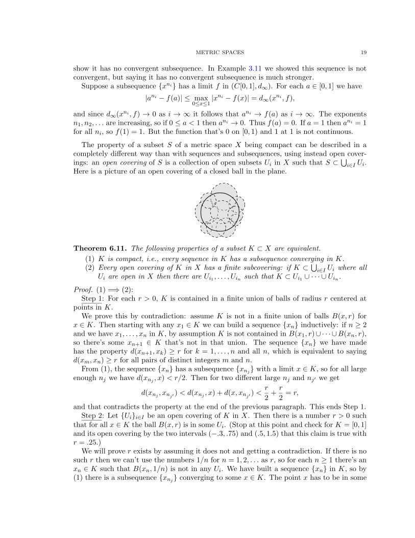
The property of a subset S of a metric space X being compact can be described in acompletely different way than with sequences and subsequences, using instead open cover-ings: an open covering of S is a collection of open subsets Ui in X such that S ⊂

⋃i∈I Ui.

Here is a picture of an open covering of a closed ball in the plane.

Theorem 6.11. The following properties of a subset K ⊂ X are equivalent.

(1) K is compact, i.e., every sequence in K has a subsequence converging in K.(2) Every open covering of K in X has a finite subcovering: if K ⊂

⋃i∈I Ui where all

Ui are open in X then there are Ui1 , . . . , Uin such that K ⊂ Ui1 ∪ · · · ∪ Uin.

Proof. (1) =⇒ (2):Step 1: For each r > 0, K is contained in a finite union of balls of radius r centered at

points in K.We prove this by contradiction: assume K is not in a finite union of balls B(x, r) for

x ∈ K. Then starting with any x1 ∈ K we can build a sequence {xn} inductively: if n ≥ 2and we have x1, . . . , xn in K, by assumption K is not contained in B(x1, r)∪ · · · ∪B(xn, r),so there’s some xn+1 ∈ K that’s not in that union. The sequence {xn} we have madehas the property d(xn+1, xk) ≥ r for k = 1, . . . , n and all n, which is equivalent to sayingd(xm, xn) ≥ r for all pairs of distinct integers m and n.

From (1), the sequence {xn} has a subsequence {xnj} with a limit x ∈ K, so for all largeenough nj we have d(xnj , x) < r/2. Then for two different large nj and nj′ we get

d(xnj , xnj′ ) < d(xnj , x) + d(x, xnj′ ) <r

2+r

2= r,

and that contradicts the property at the end of the previous paragraph. This ends Step 1.Step 2: Let {Ui}i∈I be an open covering of K in X. Then there is a number r > 0 such

that for all x ∈ K the ball B(x, r) is in some Ui. (Stop at this point and check for K = [0, 1]and its open covering by the two intervals (−.3, .75) and (.5, 1.5) that this claim is true withr = .25.)

We will prove r exists by assuming it does not and getting a contradiction. If there is nosuch r then we can’t use the numbers 1/n for n = 1, 2, . . . as r, so for each n ≥ 1 there’s anxn ∈ K such that B(xn, 1/n) is not in any Ui. We have built a sequence {xn} in K, so by(1) there is a subsequence {xnj} converging to some x ∈ K. The point x has to be in some

20 KEITH CONRAD

member of the open covering, say x ∈ Ui. Since Ui is open, we have B(x, 1/m) ⊂ Ui forsome m ≥ 1. Since nj →∞ and d(xnj , x)→ 0, for suitably large nj we have both nj > 2mand d(xnj , x) < 1/(2m). For that nj we have the implication

y ∈ B(xnj , 1/nj) =⇒ d(y, x) ≤ d(y, xnj ) + d(xnj , x) <1

nj+

1

2m<

1

2m+

1

2m=

1

m,

so B(xnj , 1/nj) ⊂ B(x, 1/m) ⊂ Ui, but that is a contradiction since no B(xn, 1/n) liesinside any member of the open covering. Thus some r exists with the desired property.

Step 3: Every open covering {Ui} of K in X has a finite subcovering containing K.

Using r as in Step 2, by Step 1 there are x1, . . . , xn ∈ K such that K ⊂⋃n

k=1B(xk, r). Bythe choice of r, each B(xk, r) is in some Ui, so K is contained in a finite union of membersof the open covering. This completes the proof that (1)⇒ (2).

(2) =⇒ (1): Let {xn} be a sequence in K. We want to show (2) implies there is aconvergent subsequence, or equivalently the sequence {xn} has a limit point in K. (Thisincludes the possibility that a point occurs infinitely often in the sequence, making it alimit of a constant subsequence.) Assume there is no limit point: no point in K is the limitof a subsequence of {xn}. Then for each y ∈ K there must be an ry > 0 such that theball B(y, ry) contains only finitely many terms from {xn}: if every ball centered at y hadinfinitely many terms from {xn} in it then we could build a subsequence tending to y byusing radius 1, 1/2, 1/3, . . ..

The balls B(y, ry) for y ∈ K are an open covering of K, so by (2) there is a finitesubcovering: K is contained in a union of finitely many of these balls. Each of these ballshas only finitely many terms from {xn} in it, so we’d get that the sequence {xn} has onlyfinitely many terms, which is absurd. �

We call condition (2) in Theorem 6.11 the open covering criterion for compactness. Itleads to a second proof that compact subsets of metric spaces are closed and bounded(Theorem 6.7).

Compact subsets are closed: (This will be similar to the proof that (2) =⇒ (1) above.)If {xn} is a sequence in K that converges to some x ∈ X then we want to show x ∈ K.Every subsequence of {xn} also tends to x, so if x is not in K then every element of Kis contained in an open ball that contains only finitely many terms of the sequence {xn}.(If this were not true then some point in K would be the limit of a subsequence, which isimpossible since all subsequences tend to x.) These open balls are an open covering of K,so by the open covering criterion for compactness we can extract a finite subcovering, butthat implies the sequence has only finitely many terms, a contradiction.

Compact subsets are bounded: One open covering of K is⋃

x∈K B(x, 1). By the open

covering criterion for compactness there is a finite subcovering, so K ⊂⋃n

k=1B(xk, 1) forsome finite set of points x1, . . . , xn in K. Thus K is in a finite union of balls, so it isbounded.

As an application of the open covering formulation of compactness, we show that allcompact subsets of R, no matter how complicated they may be, share a property withclosed bounded intervals: they contain maximum and minimum elements.

Theorem 6.12. For every nonempty compact subset K of R there are a ∈ K and b ∈ Ksuch that all x ∈ K satisfy a ≤ x ≤ b.

Proof. Suppose K does not have a maximum element. Then for each x ∈ K there is y > xin K, so x ∈ (−∞, y). Thus K ⊂

⋃y∈K(−∞, y). This open covering of K has a finite

METRIC SPACES 21

subcovering, say K ⊂ (−∞, y1) ∪ · · · ∪ (−∞, yn) with yi ∈ K. But max(y1, . . . , yn) is in Kand is not in the finite subcovering, so we have a contradiction. The proof that K has aminimum element is similar. �

If we try covering compact sets with subsets slightly different from open subsets, theremay not be a finite subcovering. Consider [0, 1] covered by the intervals [1/(n + 1), 1/n]together with {0}, or by the intervals [1/2 + 1/2n, 1] for n ≥ 2 together with [0, 1/2].

7. Connected subsets

A connected subset of a metric space is a subset that is in “one piece.” What does thatmean? It’s easier to say what it means not to be in one piece: the subset can be coveredby two disjoint open sets. For example, two closed discs in the plane that don’t overlapshould not be considered to be one piece. We can surround them by two open discs thatdon’t overlap, as shown below.

Definition 7.1. A subset S of a metric space X is called connected if whenever S ⊂ U ∪Vwhere U and V are disjoint open subsets of X, either S ⊂ U or S ⊂ V . Equivalently, S isconnected when it’s impossible to have S ⊂ U ∪ V for disjoint open subsets with S ∩U 6= ∅and S ∩ V 6= ∅.

Example 7.2. The empty set and one-point subsets are connected. Verifying other exam-ples requires work.

To say a metric space X is connected means that writing X = U ∪ V with U and Vdisjoint open subsets of X requires U or V to be empty. Since U and V are complementsin X, saying U and V are open is the same as saying U is open and closed (or “clopen”),so X being connected is equivalent to saying there are no subsets of X that are both openand closed other than ∅ and X.

Theorem 7.3. Every interval in R is connected.

Proof. Step 1: Bounded open intervals are connected. We will show (0, 1) is connected, butthe argument works with any finite endpoints.

Suppose (0, 1) ⊂ U ∪V where U and V are disjoint open subsets of R. Assume (0, 1)∩Uand (0, 1) ∩ V are both nonempty. Setting A = (0, 1) ∩ U and B = (0, 1) ∩ V , both A andB are open and we have (0, 1) = A ∪ B and A ∩ B = ∅. Since A and B are nonempty byassumption, pick a ∈ A and b ∈ B. Then a 6= b, so without loss of generality a < b.

Set S = {x ∈ A : x < b}, which is nonempty since a ∈ S. Since S is bounded above ithas a least upper bound, say `. Then a ≤ ` ≤ b, so ` ∈ [a, b] ⊂ (0, 1) = A ∪B.

If ` were in A, then ` 6= b so ` < b. Since A is an open set in R, some interval (`−ε, `+ε)would lie in A. That means all numbers very close to ` on its right lie in A, but suchnumbers (taken close enough to `) are less than b, and that contradicts ` being an upperbound on S. So ` 6∈ A.

22 KEITH CONRAD

If ` were in B, which is also an open set in R, then some interval around ` would lieentirely in B. However, since ` is the least upper bound of S there must be elements of Sin every interval of the form (`− δ, `], and S ⊂ A, so we have a contradiction. Thus ` 6∈ B.

Since ` is in neither A nor B, we have a final contradiction, so (0, 1) is connected.Step 2: Unbounded open intervals are connected. Consider the case of (0,∞). Suppose

(0,∞) ⊂ U ∪ V where U and V are disjoint open subsets of R. The interval contains 1,and without loss of generality 1 ∈ U . For all m > 1 we have (0,m) ⊂ (0,∞) ⊂ U ∪ Vand (0,m) ∩ U 6= ∅, so by connectedness of (0,m) we get (0,m) ⊂ U . Since this holdsfor all m > 1, we get (0,∞) ⊂ U . The same argument works for any unbounded openinterval with one finite endpoint. The only open interval left is R = (−∞,∞). Write it as(−∞, 2) ∪ (0,∞) and use each part separately (both contain 1) to see R is connected.

Step 3: Other intervals are connected. Let I be a non-open interval and I ⊂ U ∪ V fordisjoint open U and V in R. Let J be I without its finite endpoints, so J is an open intervaland thus we know J is connected. Since J ⊂ U ∪ V , either J ⊂ U or J ⊂ V . Withoutloss of generality, J ⊂ U . If an endpoint of I were in V then a small open interval aroundthat endpoint would be in V (since V is open in R), but this is absurd since any openinterval around an endpoint of I contains elements of J , which are all in U . Therefore finiteendpoints of I are in U too, so I ⊂ U and this proves I is connected. �

Theorem 7.4. Every nonempty subset of R that is not an interval is not connected.

Proof. Say S ⊂ R is not an interval. Then S contains two points a and b, say with a < b,and does not contain some point c in between them. Let U = (−∞, c) and V = (c,∞).Then U and V are disjoint open subsets of R, S ⊂ U ∪ V , a ∈ S ∩ U , and b ∈ S ∩ V . �

Combining the last two theorems, the nonempty connected subsets of R are precisely theintervals. There is no simple characterization of connected subsets of Rm for m > 1. Inpractice nice subsets of Rm for m > 1 are proved to be connected by proving they have astronger, more visually intuitive, property called being path-connected.

Definition 7.5. A subset S of a metric space X is called path-connected if, for every pairof points s and s′ in S, there is a continuous function p : [0, 1] → X such that p(t) ∈ S forall t, p(0) = s, and p(1) = s′.

We call such a function p a path from s to s′. Since q(t) = p(1 − t) is also continuouswith q(0) = p(1) = s′ and q(1) = p(0) = s, we can think of a path going in either direction,from s to s′ or from s′ to s.

The picture to have of a path-connected space is the inside of the blob below, where anytwo points can be linked by a path.

Theorem 7.6. Every path-connected subset of a metric space is connected.

Proving Theorem 7.6 requires information about continuous functions on metric spaces,the topic of the next section, so we defer the proof until then. Using Theorem 7.6 we

METRIC SPACES 23

can “see” right away nice solid regions or surfaces in R3 and their analogues in Rm areconnected because a path can be drawn between any two points. For example, the surfaceof a sphere or a solid ball in R3 are path-connected and thus are connected.

The converse of Theorem 7.6 in general is false: connectedness does not imply path-connectedness. An example is the “infinite broom” pictured below: it is the union of theclosed line segments Ln from (0, 0) to (1, 1/n) as n runs over positive integers together withthe (red) point (1, 0). The x-axis strictly between 0 and 1 is not part of the set. This isconnected, but there is no path from (1, 0) to any other point of the set. See [1] for a proof.

(0,0)

(1,1)

(1,1/2)

(1,1/3)(1,1/4)

(1,0)

There is an important partial converse to Theorem 7.6: for open subsets of Rm, beingconnected implies being path connected. The proof is omitted.

The concept most unlike being connected is being totally disconnected. A subset of ametric space is called totally disconnected if its only nonempty connected subsets are one-element subsets (a point is always connected). Examples of totally disconnected subsets ofthe metric space R include Z, Q, and fractals like the Cantor set. The p-adic integers andp-adic numbers, for a prime p, are important totally disconnected metric spaces in numbertheory. In Rm for m > 1 all open and closed balls are connected, which is a nice analogywith the one-dimensional case, but in a totally disconnected metric space no open or closedballs are connected (aside from closed balls of radius 0, i.e., points).

8. Continuous functions between metric spaces

Up until now the only limits we have discussed in metric spaces were limits of sequences.Now we turn to limiting values of functions defined on a metric space, and specifically con-tinuous functions on a metric space. This is where we will see the importance of connectedsets and compact sets.

Specifically, we want to prove the following two properties of continuous functions.

Theorem 8.1 (Intermediate Value Theorem). Let I be an interval and f : I → R becontinuous. If a < b in I and f(a) 6= f(b) then for every y strictly between f(a) and f(b)there is c ∈ (a, b) such that f(c) = y.

Theorem 8.2 (Extreme Value Theorem). Every continuous real-valued function on a closedbounded interval has maximum and minimum values: if f : [a, b] → R is continuous on a

24 KEITH CONRAD

closed bounded interval then there are m and M such that (i) m ≤ f(x) ≤ M for all x in[a, b] and (ii) m and M are values of f(x).

The Extreme Value Theorem justifies the definition of the metric d∞ on C[0, 1] back inSection 2 as a maximum value of a continuous function on [0, 1]. In contrast to the ExtremeValue Theorem, a continuous bounded function on an open interval doesn’t have to havea maximum value, such as 1/x on (1, 2). Its values are bounded above by 1, but no valueof the function is greater than all other values. The difference between closed boundedintervals and open intervals is that closed bounded intervals are compact, and we’ll see thatis what makes the Extreme Value Theorem work.

Before we prove theorems about continuous functions we have to define continuous func-tions. The definition of continuity for a real-valued function on an interval, usually called the(ε, δ)-definition, goes as follows. For a real number a and a real-valued function f(x) definedon an interval containing a, we say f(x) is continuous at a and write limx→a f(x) = f(a) iffor every ε > 0 there is a δ = δa,ε > 0 such that

|x− a| < δ =⇒ |f(x)− f(a)| < ε.

If we have a real-valued function f : Rm → R, and a ∈ Rm, then we say f(x) is continuousat a and write limx→a f(x) = f(a) if for every ε > 0 there is a δ = δa,ε > 0 such that

||x− a|| < δ =⇒ |f(x)− f(a)| < ε.

Notice the different distances being used here, one on Rm (where the function is defined)and one on R (where the function takes its values).

Definition 8.3. A function f : X → Y between two metric spaces is called continuous ata ∈ X if for every ε > 0 there is a δ = δa,ε > 0 such that

dX(x, a) < δ =⇒ dY (f(x), f(a)) < ε.

If f is continuous at each point of X then we say f is continuous on X.

As a warm-up, let’s show every metric is a continuous function on its metric space whenwe view it as a function of one of its variables, keeping the other one fixed.

Theorem 8.4. For any metric space (X, d) and point c ∈ X, the function fc : X → R thatis “distance to c”, namely fc(x) = d(c, x), is continuous.

Proof. Pick a ∈ X and ε > 0. We need a δ > 0 such that

d(x, a) < δ =⇒ |fc(x)− fc(a)| < ε.

The inequality on the right says |d(c, x)− d(c, a)| < ε.Using the triangle inequality in two ways,

d(c, a) ≤ d(c, x) + d(x, a) and d(c, x) ≤ d(c, a) + d(a, x),

so

d(c, a)− d(c, x) ≤ d(x, a) and d(c, x)− d(c, a) ≤ d(a, x).

Thus |d(c, x)− d(c, a)| ≤ d(x, a). Therefore

d(x, a) < ε =⇒ |d(c, x)− d(c, a)| ≤ d(x, a) < ε

so we can use δ = ε. �

METRIC SPACES 25

Remark 8.5. By a two-way triangle inequality argument like the one used in this proof,show

|d(x, y)− d(xn, yn)| ≤ d(x, xn) + d(y, yn)

for xn, x, yn, y ∈ X. Therefore if xn → x and yn → y in X then this inequality showsd(xn, yn)→ d(x, y), an intuitively reasonable property.

Theorem 8.6. For any metric space (X, d), the identity function X → X where x 7→ x iscontinuous.

Proof. This is straightforward, using δ = ε. �

Theorem 8.7. Addition and multiplication, as functions R2 → R given by A(x, y) = x+yand M(x, y) = xy, are both continuous.

Proof. First we prove continuity of addition. Pick (a, b) ∈ R2 and ε > 0. We need δ > 0such that

||(x, y)− (a, b)|| < δ =⇒ |A(x, y)−A(a, b)| < ε.

We will use δ = ε/2.

If ||(x, y)− (a, b)|| < ε/2 then√

(x− a)2 + (y − b)2 < ε/2, so |x− a| < ε/2 and |y− b| <ε/2. Then

|A(x, y)−A(a, b)| = |(x+ y)− (a+ b)| ≤ |x− a|+ |y − b| < ε

2+ε

2= ε.

To prove multiplication is continuous we estimate |M(x, y)−M(a, b)| = |xy − ab|:

|xy − ab| = |(x− a)y + (y − b)a|= |(x− a)(y − b) + (x− a)b+ (y − b)a|≤ |x− a||y − b|+ |x− a|b+ |y − b|a.

Thus if |x− a| < δ and |y − b| < δ, then |xy − ab| < δ2 + δb+ δa = δ(δ + b+ a). If

(8.1) δ ≤ 1 and δ ≤ ε

1 + a+ b

then δ(δ+ b+ a) ≤ δ(1 + b+ a) ≤ ε. So pick δ = min(1, ε/(1 + a+ b)) to make δ satisfy thetwo inequalities in (8.1). Then

||(x, y)− (a, b)|| < δ =⇒ |x− a|, |y − b| < δ

and our calculations above imply |xy − ab| < ε. �

In this proof notice that for continuity of multiplication our choice of δ depends not onlyon ε, but also on the point (a, b) where we are checking continuity. This is typical: inpractice the choice for δ may depend on the point at which we are proving continuity. (Inthe definition of continuity at a, we wrote δ = δa,ε.) This did not happen for addition,where δ = ε/2 everywhere. Such “independence of the point” is special; it will lead later tothe concept of uniform continuity.

Theorem 8.8. Any composition of continuous functions on metric spaces is continuous:if f : X → Y and g : Y → Z are continuous then the composite function g ◦ f : X → Z iscontinuous.

26 KEITH CONRAD

Proof. Pick a ∈ X and ε > 0. We have (g ◦ f)(a) = g(f(a)). By the definition of continuityof g at f(a), there’s an η > 0 (depending on f(a) and ε) such that

(8.2) dY (y, f(a)) < η =⇒ dZ(g(y), g(f(a))) < ε.

By the definition of continuity of f at a, there’s a δ > 0 (depending on η and a) such that

dX(x, a) < δ =⇒ dY (f(x), f(a)) < η,

and by (8.2) that last inequality implies dZ(g(f(x)), g(f(a))) < ε. �

Just as compactness has a formulation in terms of open sets rather than sequences (The-orem 6.11), using open coverings, continuity of a function on a metric space also has aformulation in terms of open sets rather than ε’s and δ’s. More precisely, continuity of afunction can be expressed in terms of inverse images of open sets. For a function f : X → Yand a subset S ⊂ Y , the inverse image f−1(S) means {x ∈ X : f(x) ∈ S}. An inverse imageof a function on a subset makes sense even if the function is not invertible. For example, iff : R→ R by f(x) = x2 then

f−1((0, 1)) = (−1, 0) ∪ (0, 1) f−1((−2, 2)) = (−√

2,√

2),

f−1((1, 2)) = (−√

2,−1) ∪ (1,√

2), f−1((−1, 0)) = ∅.Inverse images of subsets under a function behave well for all set-theoretic operations: if

f : X → Y is a function then for subsets S and T in Y ,

f−1(S ∩ T ) = f−1(S) ∩ f−1(T ), f−1(S ∪ T ) = f−1(S) ∪ f−1(T ),

S ⊂ T =⇒ f−1(S) ⊂ f−1(T ), f−1(S − T ) = f−1(S)− f−1(T ),

where S − T = {s ∈ S : s 6∈ T}. (For example, if S = {0, 1} and T = {1, 2} thenS − T = {0}.) We will use these properties without comment below.8 In particular,f−1(Y − S) = X − f−1(S), so inverse images send complements to complements.

Theorem 8.9. A function f : X → Y between two metric spaces is continuous if and onlyif the inverse image of every open set in Y is open in X: for all open U in Y , the setf−1(U) = {x ∈ X : f(x) ∈ U} is open in X.

Proof. First suppose f fits the (ε, δ)-definition of continuity on X, so f is continuous ateach element of X. For every open set U ⊂ Y we want to show f−1(U) is open in X.

If f−1(U) = ∅ then f−1(U) is open by our convention that the empty set is open, sosuppose f−1(U) 6= ∅. Pick a ∈ f−1(U), so f(a) ∈ U . Since U is open in Y there’ssome ε > 0 such that B(f(a), ε) ⊂ U . By the (ε, δ)-definition of continuity at a, thereis a δ > 0 such that dX(x, a) < δ =⇒ dY (f(x), f(a)) < ε. This implication is sayingf(B(a, δ)) ⊂ B(f(a), ε), so B(a, δ) ⊂ f−1(B(f(a), ε)) ⊂ f−1(U). This shows each a inf−1(U) is contained in an open ball that’s contained in f−1(U), so f−1(U) is open in X.

Now we prove the converse. Suppose for all U open in Y we have f−1(U) open in X. Forevery a ∈ X we will prove f is continuous at a. For each ε > 0, the open ball B(f(a), ε) inY is open, so using B(f(a), ε) as U the inverse image f−1(B(f(a), ε)) is open in X and thisinverse image includes a. Thus there’s a δ > 0 such that B(a, δ) ⊂ f−1(B(f(a), ε)), andunwinding the notation this containment is saying that if dX(a, x) < δ then dY (f(a), f(x)) <ε. That is exactly the (ε, δ)-definition of continuity of f at a. �

8Analogous formulas for images of subsets are true for unions and containments but false for intersectionsand complements: use f(x) = x2 with A = {1, 2} and B = {1,−2} to see f(A ∩ B) 6= f(A) ∩ f(B) andf(A−B) 6= f(A)− f(B).

METRIC SPACES 27

It is false that continuous functions always send open sets to open sets. For example, thesquaring function R → R sends (−1, 1) to [0, 1). Continuity aligns with inverse images ofopen sets, not images of open sets. C’est la vie.

Remark 8.10. Theorem 8.9 is an open-set formulation of continuity on a whole set, notat a particular point. There is an open-set formulation of continuity at a point: f : X → Yis continuous at a if and only if for all open U ⊂ Y containing f(a) there is an open V ⊂ Xcontaining a such that f(V ) ⊂ U . Checking this matches the (ε, δ)-definition of continuityat a is left to the reader.

Corollary 8.11. A function f : X → Y between two metric spaces is continuous if andonly if the inverse image of every closed set in Y is closed in X.

Proof. Theorem 5.17 tells us that open and closed subsets are complementary to each other.For any closed subset C of Y , U = Y −C is open and f−1(U) = f−1(Y −C) = X−f−1(C).Therefore f−1(C) is closed if and only if f−1(U) is open, so Theorem 8.9 tells us continuityof f is equivalent to f−1 sending closed subsets to closed subsets. �

Example 8.12. In R3, the sphere S2 = {(x, y, z) ∈ R3 : x2 + y2 + z2 = 1} is closed. Thiscan be proved directly using sequences in S2 or by observing that f(x, y, z) = x2 + y2 + z2

is a continuous function R3 → R and S2 = f−1(1) with the one-point set {1} in R beingclosed.

To illustrate the open-set formulation of continuity of a function, we prove Theorem 7.6:path-connected sets are connected.

Proof. Let S be a path-connected subset of a metric space X. We will use paths in S to showthat if S is not connected then [0, 1] is not connected, which of course is a contradiction, soS has to be connected.

Suppose S is not connected, so we have S ⊂ U ∪V where U and V are nonempty disjointopen subsets of X. Pick s ∈ S ∩ U and s′ ∈ S ∩ V . There is a path p : [0, 1] → S wherep(0) = s and p(1) = s′. The partition of S into S ∩ U and S ∩ V leads via this path to apartition of [0, 1]: [0, 1] = p−1(U) ∪ p−1(V ). Set A = p−1(U) and B = p−1(V ). Both areopen subsets of [0, 1] since p is continuous.9

Note 0 ∈ A and 1 ∈ B, so A and B are nonempty. Obviously A and B are disjoint, sinceno point in [0, 1] can have its p-value in both U and V . Thus the equation [0, 1] = A ∪ Bexhibits [0, 1] as a disjoint union of two nonempty open subsets of [0, 1], which contradictsthe connectedness of [0, 1]. �

Next we reprove Theorem 8.8 using open sets instead of ε’s and δ’s.

Proof. Let U be an arbitrary open set in Z. Then

(g ◦ f)−1(U) = {x ∈ X : (g ◦ f)(x) ∈ U}= {x ∈ X : g(f(x)) ∈ U}= {x ∈ X : f(x) ∈ g−1(U)}= f−1(g−1(U)).

By continuity of g, g−1(U) is open in Y , and by continuity of f , f−1(g−1(U)) is open in X.Thus g ◦ f is continuous. �

9In [0, 1], intervals of the form [0, ε) are open! This is the ball B(0, ε) in the metric space [0, 1], even thoughthe same interval is not open in R.

28 KEITH CONRAD

Think about why this proof of Theorem 8.8 and the first proof of Theorem 8.8 really arethe same argument even though at first glance they might look different. Mathematiciansconsider the second proof, using open sets, to be more elegant.

As a substantial application of continuity being preserved under composition, we willprove polynomials with real coefficients are continuous. We’ll need one lemma.

Lemma 8.13. Let f : R→ R and g : R→ R. If f and g are continuous then the functionR→ R2 given by x 7→ (f(x), g(x)) is continuous.

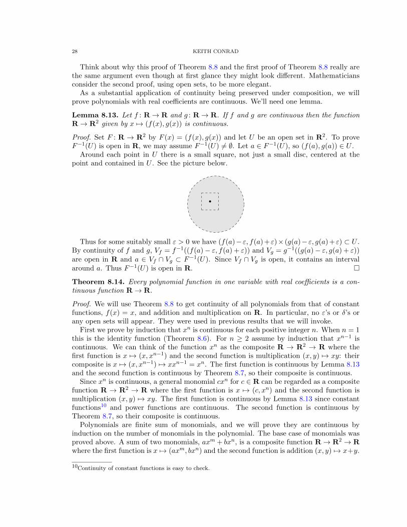
Proof. Set F : R → R2 by F (x) = (f(x), g(x)) and let U be an open set in R2. To proveF−1(U) is open in R, we may assume F−1(U) 6= ∅. Let a ∈ F−1(U), so (f(a), g(a)) ∈ U .

Around each point in U there is a small square, not just a small disc, centered at thepoint and contained in U . See the picture below.

Thus for some suitably small ε > 0 we have (f(a)−ε, f(a)+ε)× (g(a)−ε, g(a)+ε) ⊂ U .By continuity of f and g, Vf = f−1((f(a)− ε, f(a) + ε)) and Vg = g−1((g(a)− ε, g(a) + ε))are open in R and a ∈ Vf ∩ Vg ⊂ F−1(U). Since Vf ∩ Vg is open, it contains an intervalaround a. Thus F−1(U) is open in R. �

Theorem 8.14. Every polynomial function in one variable with real coefficients is a con-tinuous function R→ R.

Proof. We will use Theorem 8.8 to get continuity of all polynomials from that of constantfunctions, f(x) = x, and addition and multiplication on R. In particular, no ε’s or δ’s orany open sets will appear. They were used in previous results that we will invoke.

First we prove by induction that xn is continuous for each positive integer n. When n = 1this is the identity function (Theorem 8.6). For n ≥ 2 assume by induction that xn−1 iscontinuous. We can think of the function xn as the composite R → R2 → R where thefirst function is x 7→ (x, xn−1) and the second function is multiplication (x, y) 7→ xy: theircomposite is x 7→ (x, xn−1) 7→ xxn−1 = xn. The first function is continuous by Lemma 8.13and the second function is continuous by Theorem 8.7, so their composite is continuous.

Since xn is continuous, a general monomial cxn for c ∈ R can be regarded as a compositefunction R → R2 → R where the first function is x 7→ (c, xn) and the second function ismultiplication (x, y) 7→ xy. The first function is continuous by Lemma 8.13 since constantfunctions10 and power functions are continuous. The second function is continuous byTheorem 8.7, so their composite is continuous.

Polynomials are finite sum of monomials, and we will prove they are continuous byinduction on the number of monomials in the polynomial. The base case of monomials wasproved above. A sum of two monomials, axm + bxn, is a composite function R→ R2 → Rwhere the first function is x 7→ (axm, bxn) and the second function is addition (x, y) 7→ x+y.

10Continuity of constant functions is easy to check.

METRIC SPACES 29

Both of these functions are continuous by the base case, Lemma 8.13, and Theorem 8.7, sotheir composite is continuous. The general inductive step is left to the reader. �

Theorem 8.15. Let f : X → Y be continuous. If S ⊂ X is compact then f(S) is compactin Y .

Proof. We will give two proofs, one using the convergent subsequence description of com-pactness and the other using the open covering description of compactness.

First proof: Let {yn} be a sequence in f(S), so we can write yn = f(xn) for somexn ∈ S. By compactness of S, the sequence {xn} in S has a convergent subsequence, sayxni → x ∈ S. Then by continuity, f(xni)→ f(x), so yni → f(x) ∈ f(S). We proved everysequence in f(S) has a convergent subsequence, so f(S) is compact.

Second proof: Let {Ui} be an open covering of f(S), so f(S) ⊂⋃

i∈I Ui in Y . Then

S ⊂⋃

i∈I f−1(Ui), and each f−1(Ui) is open in X, so {f−1(Ui)} is an open covering of S

in X. By compactness of S there is a finite subcovering, say S ⊂ f−1(U1) ∪ · · · ∪ f−1(Un).Then f(S) ⊂ U1 ∪ · · · ∪ Un, so every open covering of f(S) has a finite subcovering. �

Theorem 8.16. Let f : X → Y be continuous. If S ⊂ X is connected then f(S) is connectedin Y .

Proof. Suppose f(S) ⊂ U ∪ V where U and V are disjoint open subsets of Y . ThenS ⊂ f−1(U ∪ V ) = f−1(U) ∪ f−1(V ). The inverse images f−1(U) and f−1(V ) are openin X, and they are disjoint since U and V are disjoint (if a ∈ f−1(U) ∩ f−1(V ) thenf(a) ∈ U ∩ V = ∅, a contradiction). Since S is connected, we have either S ⊂ f−1(U) orS ⊂ f−1(V ), so f(S) ⊂ U or f(S) ⊂ V . Thus f(S) is connected. �

With Theorems 8.15 and 8.16 and our knowledge of connected and compact intervals inR, we can now prove the Intermediate Value Theorem (Theorem 8.1) and Extreme ValueTheorem (Theorem 8.2).

Proof. (Intermediate Value Theorem) Let I be an interval and f : I → R be continuous.Suppose a < b in I with f(a) 6= f(b). The image f([a, b]) is connected in R by Theorem8.16, so it must be an interval. Any interval containing f(a) and f(b) contains all numbersbetween them, so every y strictly between f(a) and f(b) is f(c) for some c ∈ [a, b] ⊂ I, andc is not a or b since y is not f(a) or f(b). �

Proof. (Extreme Value Theorem) Let f : [a, b] → R be continuous. Since [a, b] is compactand connected, f([a, b]) is compact and connected by Theorems 8.15 and 8.16. The con-nected subsets of R are intervals, and compact intervals are closed and bounded, so f([a, b])must have the form [m,M ] for some m,M ∈ R. The conclusions of the Extreme ValueTheorem follow from this. �

Theorem 8.17. If X is a compact metric space and f : X → R is a continuous functionwith positive values everywhere then there is some c > 0 such that f(x) ≥ c for all x ∈ X,and we can take c = f(x0) for some x0 ∈ X.

Proof. The image f(X) is compact in R by Theorem 8.15, so Theorem 6.12 implies thereis an x0 ∈ X such that f(x) ≥ f(x0) for all x ∈ X. Set c = f(x0) > 0. �

Positive continuous functions on non-compact spaces need not have a positive lowerbound. Consider 1/x as a function (0,∞) → R. There is no c > 0 such that 1/x ≥ c > 0for all x > 0.

30 KEITH CONRAD

Corollary 8.18. If K is a compact subset of the metric space X then for each x ∈ X thedistance from x to the elements of K has a minimum: there is some y0 ∈ K such thatd(x, y) ≥ d(x, y0) for all y ∈ K.

Proof. Let f : K → R by f(y) = d(x, y). This is continuous by Theorem 8.4 so its imagef(K) is compact in R. By Theorem 6.12 (with K in that theorem being f(K) here) somevalue d(x, y0) for y0 ∈ K is a minimum value of f . �

We now turn to the final topic about continuous functions that we’ll discuss. It is animportant refinement of continuity.

Definition 8.19. A function f : X → Y between two metric spaces is called uniformlycontinuous if for every ε > 0 there is a δ = δε > 0 such that for all a ∈ X,

dX(x, a) < δ =⇒ dY (f(x), f(a)) < ε.

Uniform continuity is a special kind of continuity. The difference is that uniform continu-ity says the value of δ can be chosen in terms of ε alone, independently of a choice of pointa (so we can choose δ “uniformly in a,” hence the name). Look at the graphs of y = x2

and y = 2x below. In each case we use ε = .75 and indicate in red the largest δ-intervalsaround a = 1 and a = 2 on the x-axis that make |x − a| < δ =⇒ |f(x) − f(a)| < .75. Forf(x) = x2 we need a shorter interval around a = 2 to keep the f -values within .75 of f(2)than we need around a = 1 to keep f -values within .75 of f(1), but for f(x) = 2x intervalsof the same radius around 1 and 2 lead to intervals of the same radius around f(1) and f(2).Linear functions on R are uniformly continuous while x2 on R is not uniformly continuous.

x

y

2

4

y = x2

1

1

x

y

1 2

2

4

y = 2x

It is instructive to compare the definitions of continuity and uniform continuity usingquantifier notation. Continuity of a function f : X → Y says

∀a ∈ X ∀ε > 0 ∃ δ > 0 s.t. ∀x ∈ X, dX(x, a) < δ =⇒ dY (f(x), f(a)) < ε.

while uniform continuity of a function f : X → Y says

∀ε > 0 ∃ δ > 0 s.t. ∀a ∈ X ∀x ∈ X, dX(x, a) < δ =⇒ dY (f(x), f(a)) < ε.

The only difference is where “∀a ∈ X” appears: in continuity it is at the start while inuniform continuity it is after δ. The order of quantifiers has a substantial impact on whatsomething means. A simpler example: it’s true that ∀x ∈ R s.t. x > 0∃ y ∈ R s.t. y2 = x

METRIC SPACES 31

(every positive real number has a real square root), but it’s false that ∃ y ∈ R s.t. ∀x ∈ R s.t.x > 0, y2 = x (there’s a universal square root of all positive numbers?). Definitions in realanalysis have many nested quantifiers, so it’s understandable why even a mathematician ofthe stature of Cauchy, who introduced the (ε, δ)-definition11 of continuity, confused it withuniform continuity in proofs.

Unlike continuity, uniform continuity can’t be described as a property at individual pointsof the domain (why?). Also unlike continuity, there no way to convert uniform continuityinto a statement about general open subsets.12 Proofs about uniform continuity use (ε, δ)-language.

The last general comment we have about uniform continuity is that in its definition aand x play symmetric roles (they are quantified at the same time, unlike in the definitionof continuity), so we can express uniform continuity in a way that puts a and x on an equalfooting, which we therefore will write as x and x′. A function f : X → Y is called uniformlycontinuous if for every ε > 0 there is a δ = δε > 0 such that for all x, x′ ∈ X,

dX(x, x′) < δ =⇒ dY (f(x), f(x′)) < ε.

This is the formulation of uniform continuity that we will use below. (Note: we are notsaying all x and x′ satisfy dX(x, x′) < δ, but rather that they satisfy the total implicationwritten above: if dX(x, x′) < δ then dY (f(x), f(x′)) < ε.)

Example 8.20. We saw before that x2 is not uniformly continuous on R, since for a givenε the function values stay within ε of each other at larger numbers that are within δ ofeach other only if δ is made progressively smaller. We can’t use the same δ as the pointsget too big. But if we restrict ourselves to a bounded domain then x2 becomes uniformlycontinuous. For instance, on the interval [−b, b] where b > 0,

|x− x′| < δ =⇒ |x2 − x′2| = |x− x′||x+ x′| < δ(|x|+ |x′|) ≤ δ(2b),so to make |x2 − x′2| < ε when |x− x′| < δ in [−b, b] we can use δ = ε/(2b).

Example 8.21. For a > 0 the function 1/x on [a,∞) is uniformly continuous:

|x− x′| < δ =⇒∣∣∣∣1x − 1

x′

∣∣∣∣ =|x′ − x||x||x′|

<δ

a2,

so we can make |1/x− 1/x′| < ε if |x− x′| < δ in [a,∞) using δ = a2ε.

Example 8.22. For a metric space (X, d) and c ∈ X, the function fc(x) = d(c, x) isuniformly continuous on X. This comes from the proof of Theorem 8.4, where we could useδ = ε independently of the point x at which we were checking continuity of fc.

Here is the fundamental property that gives rise to uniformly continuous functions.

Theorem 8.23. A continuous function f : X → Y from a compact metric space to anymetric space is uniformly continuous.

This doesn’t say continuous functions can’t be uniformly continuous on non-compactmetric spaces (see Example 8.21), only that they must be uniformly continuous on compactmetric spaces.

11Bolzano had developed similar ideas earlier, but his work was not widely read until after Cauchy.12A partial translation into open sets is possible, but the family of all balls of a common radius has to begiven a special status, called a “uniformity”. We don’t get into that here.

32 KEITH CONRAD

Proof. We prove the theorem in two ways, using the subsequence description of compactnessand using the open covering description of compactness.

First proof (using subsequences): Our argument will be by contradiction, starting withthe assumption that f is not uniformly continuous. Figuring out what it means not to beuniformly continuous is going to take up the bulk of the proof!

One way to say f is not uniformly continuous is to say it is not true that for every ε > 0there is a δ > 0 such that all x and x′ in X satisfy dX(x, x′) < δ =⇒ dY (f(x), f(x′)) < ε.But this is not really progress; adding “It is not true that” to the start of a sentence inorder to negate it doesn’t usually let us understand the meaning of the negation.

The negation of a statement of the form “for every ε > 0 there is a δ > 0 such thatsomething happens” is “there is an ε > 0 such that for all δ > 0 the thing does nothappen.” Using quantifier notation, for a proposition P the negation of

∀ε > 0 ∃ δ > 0 s.t. P

is

∃ ε > 0 s.t. ∀δ > 0 ∼ P ,

where ∼ P is the negation of P . Negating turns ∀ into ∃ and vice versa.For us, P is “all x and x′ in X satisfy dX(x, x′) < δ =⇒ dY (f(x), f(x′)) < ε.” Its negation

is “some x and x′ in X satisfy dX(x, x′) < δ and dY (f(x), f(x′)) ≥ ε”. (Observe “< ε”turned into “≥ ε” at the end, as a negation.) Putting everything together, the negation off being uniformly continuous says:

There is ε>0 s.t. for all δ>0, an x and x′ in X satisfy dX(x, x′)<δ & dY (f(x), f(x′))≥ε.

The numbers x and x′ here may depend on δ (each δ needs an example of x and x′).Now that we can express what it means not to be uniformly continuous, assume f is not

uniformly continuous. For the special ε that occurs, use δ = 1/n with n = 1, 2, 3, . . .: foreach n there are xn and x′n in X such that dX(xn, x

′n) < 1/n and dY (f(xn), f(x′n)) ≥ ε. We

have built two sequences in X: {xn} and {x′n}. By compactness of X, some subsequence{xni} of {xn} converges in X, say to x. Also x′ni

→ x by Theorem 3.8. By continuityof f , f(xni) → f(x) and f(x′ni

) → f(x), so dY (f(xni), f(x′ni)) → 0. This contradicts the

inequality dY (f(xn), f(x′n)) ≥ ε for all n, so we’re done.Second proof (using open coverings): This proof will not be by contradiction. Pick ε > 0.

For each x ∈ X, continuity of f at x implies there is some δx > 0 such that

(8.3) dX(x, x′) < δx =⇒ dY (f(x), f(x′)) <ε

2.

The balls B(x, δx) are an open covering of X, so by compactness there is a finite subcovering,say by B(x1, δx1), . . . , B(xn, δxn). Set δ = min(δx1/2, . . . , δxn/2) > 0.

Pick x and x′ in X with dX(x, x′) < δ. We have x ∈ B(xi, δxi/2) for some i = 1, . . . , n.Then dX(x, xi) < δxi/2 < δxi , so dY (f(x), f(xi)) < ε/2 by (8.3). Also

dX(x′, xi) ≤ dX(x′, x) + dX(x, xi) < δ +δxi

2≤ δxi

2+δxi

2= δxi ,

so dY (f(x′), f(xi)) < ε/2 by (8.3). Thus

dY (f(x), f(x′)) ≤ dY (f(x), f(xi)) + dY (f(xi), f(x′)) <ε

2+ε

2= ε.

�

METRIC SPACES 33

To illustrate the better control that is built into uniform continuity compared to continu-ity, we will prove uniformly continuous functions can be extended from dense subsets to thewhole space. We need a lemma about a basic property of uniformly continuous functionsthat is not generally true of continuous functions.

Lemma 8.24. If f : X → Y is uniformly continuous and {xn} is a Cauchy sequence in Xthen {f(xn)} is a Cauchy sequence in Y .

Proof. Pick ε > 0. By uniform continuity there is a δ > 0 such that for all x and x′ inX satisfying dX(x, x′) < δ we have dY (f(x), f(x′)) < ε. Since {xn} is Cauchy in X, usingthe value of δ there is an N ≥ 1 such that m,n ≥ N =⇒ dX(xm, xn) < δ. Then uniformcontinuity implies dY (f(xm), f(xn)) < ε for m,n ≥ N , so {f(xn)} is Cauchy in Y . �

In contrast to this, a continuous function might not send Cauchy sequences to Cauchysequences: 1/x maps (0,∞) → R and {1/n} is Cauchy in (0,∞) but {1/(1/n)} = {n} isnot Cauchy in R. Of course continuous functions send convergent sequences to convergentsequences, by definition!

Theorem 8.25. Let X and Y be metric spaces, with Y complete. For any dense subsetD of X, every uniformly continuous function f : D → Y uniquely extends to a continuous

function f : X → Y , defined by f(x) = limn→∞ f(xn) for any sequence {xn} in D that

converges to x. Moreover, f is uniformly continuous.

Proof. If f has an extension to a continuous function f on X then for each x ∈ X, f(x)has to equal limn→∞ f(xn) for any sequence xn in D that converges to x (such a sequencein D exists for each x since D is dense in X). Therefore the uniqueness of a continuousextension is clear. What we have to address is the existence:

(1) If xn → x and x′n → x with xn and x′n in D for all n, why do the sequences {f(xn)}and {f(x′n)} have a common limit?

(2) Why is the function f : X → Y defined by f(x) = limn→∞ f(xn), if xn → x in D,continuous?

For x ∈ X, let {xn} be a sequence in D such that xn → x. Then {xn} is a Cauchysequence in D. By Lemma 8.24 for the uniformly continuous function f : D → Y , {f(xn)}is a Cauchy sequence in Y , so this sequence has a limit since Y is complete.

We want to label limn→∞ f(xn) as f(x), but why is the limit well-defined from x: if {xn}and {x′n} are sequences in D that tend to x, why do the convergent sequences {f(xn)} and{f(x′n)} in Y have the same limit? It suffices to show dY (f(xn), f(x′n))→ 0 (Theorem 3.8).That is, for every ε > 0 we want an N such that n ≥ N =⇒ dY (f(xn), f(x′n)) < ε.

From uniform continuity of f on D, for each ε > 0 there is a δ > 0 such that for alla and b in D, dX(a, b) < δ =⇒ dY (f(a), f(b)) < ε. Since xn → x and x′n → x we havedX(xn, x

′n) → 0, so there’s some N such that n ≥ N =⇒ dX(xn, x

′n) < δ. Therefore

n ≥ N =⇒ dY (f(xn), f(x′n)) < ε, which is what we wanted. This completes the proof thatthe definition

f(x) := limn→∞

f(xn) ∈ Y

for x ∈ X and any sequence {xn} in D with xn → x is independent of the choice of {xn}. In

particular, if x ∈ D then use xn = x for all n to see f(x) = limn→∞ f(xn) = limn→∞ f(x) =

f(x). Thus on D, f restricts to f .

34 KEITH CONRAD

It remains to show f is continuous. We will use uniform continuity of f to prove f is infact uniformly continuous. This will be an ε/3 argument.

By uniform continuity of f on D, for every ε > 0 there is δ > 0 such that

(8.4) dX(a, b) < δ in D =⇒ dY (f(a), f(b)) <ε

3.

Suppose x and x′ in X satisfy dX(x, x′) < δ. There are sequences {xn} and {x′n} in D suchthat xn → x and x′n → x′. Then

dY (f(x), f(x′)) ≤ dY (f(x), f(xn)) + dY (f(xn), f(x′n)) + dY (f(x′n), f(x′))

= dY (f(x), f(xn)) + dY (f(xn), f(x′n)) + dY (f(x′n), f(x′)).

Since, by definition, f(x) is the limit of the f(xn) and f(x′) is the limit of the f(x′n), for

large enough n both dY (f(x), f(xn)) and dY (f(x′n), f(x′)) are less than ε/3. Also for largeenough n, dX(xn, x

′n) < δ since xn and x′n both tend to x, so dY (f(xn), f(x′n)) < ε/3 for

large enough n by (8.4). Plugging this all into the above inequality, for large enough n

dY (f(x), f(x′)) ≤ dY (f(x), f(xn)) + dY (f(xn), f(x′n)) + dY (f(x′n), f(x′)) <ε

3+ε

3+ε

3= ε.

�

Example 8.26. While 1/x is uniformly continuous as a function [1,∞) → R (Example8.21 with a = 1), it is not uniformly continuous as a function (0, 1]→ R: if it were uniformlycontinuous on (0, 1], then it would extend to a continuous function on [0, 1], which of courseit does not.

The reader should show 1/x is not uniformly continuous on (0, 1] directly from the defi-nition of uniform continuity, without needing a result like Theorem 8.25. Use the negationof uniform continuity from the proof of Theorem 8.23.

Example 8.27. The function f(x) = 1/(x2 − 2) on Q ∩ [1, 2] is continuous, but it is notuniformly continuous: if it were uniformly continuous then the function would extend to acontinuous function on [1, 2], which is clearly false due to a problem at x =

√2.

Example 8.28. As a positive application of Theorem 8.23, for each a > 1 we use thetheorem to construct13 ax for irrational x > 0 from the case of rational x ≥ 0 and show ax

is continuous in x. To use Theorem 8.23 we restrict attention to bounded intervals of x.We will take for granted as background the existence of positive rational powers. For

each r ∈ Q with r > 0, written as the ratio of positive integers m/n, the number ar = am/n

is the unique solution of xn = am in (1,∞). Its existence and uniqueness follow from theIntermediate Value Theorem since xn is continuous, increasing, and unbounded as x→∞with value 1 at x = 1.

Claim 1: For positive integers N , 1 < a1/N < 1 + (a− 1)/N .Proof: For h > 0, (1 + h)N > 1 + Nh by the Binomial Theorem and 1 + Nh ≥ a if

h ≥ (a − 1)/N . Thus h ≥ (a − 1)/N =⇒ (1 + h)N > a, so if a1/N = 1 + h then we see

a1/N − 1 = h < (a− 1)/N , so a1/N < 1 + (a− 1)/N .

From Claim 1, a1/N → 1 as N →∞ in Z.Take for granted that aras = ar+s for rational r, s ≥ 0. From this it follows that

0 ≤ r < s =⇒ ar < as: s − r > 0 =⇒ as−r > 1 =⇒ as = aras−r > ar. Then ar → 1 asr → 0+ through rational numbers because it is true when r = 1/N and ar is increasing.

13All we do could be adapted to 0 < a < 1, but we stick to a > 1 to keep the notation simple.

METRIC SPACES 35

Claim 2: On each bounded interval Q∩ [0,M ] for integers M ≥ 1, the function f(r) = ar

is uniformly continuous.Proof: Pick a positive integer N and let r, s ∈ Q ∩ [0,M ] satisfy |r − s| < 1/N . Suppose

r ≥ s. Then

f(r)− f(s) = ar − as = as(ar−s − 1) =⇒ |f(r)− f(s)| ≤ aM (ar−s − 1).

From r − s < 1/N we get 1 ≤ ar−s < a1/N < 1 + (a− 1)/N by Claim 1, so 0 ≤ ar−s − 1 <

(a− 1)/N . Thus |f(r)− f(s)| ≤ aM (a−1)N . If instead r < s then we get the same bound by

switching the roles of r and s. Thus

r, s ∈ Q ∩ [0,M ] and |r − s| < 1

N=⇒ |f(r)− f(s)| ≤ aM (a− 1)

N.

This implies uniform continuity on Q ∩ [0,M ]: for ε > 0 let δ = 1/N where N is chosenlarge enough that aM (a− 1)/N < ε.

By Claim 2 and Theorem 8.23, for each integer M ≥ 1 the function f(x) = ax onQ ∩ [0,M ] uniquely extends to a uniformly continuous function on [0,M ], which we will

also denoted by ax. For example, a√2 is the limit of ar for rationals r tending to

√2. The

function ax on [0,M ] for larger M has to agree with ax on [0,M ] for smaller M since there’sat most one continuous extension on each [0,M ]. Therefore letting M →∞ we get a singlecontinuous function ax for all x ≥ 0 that agrees with the originally defined ax when theexponent x is rational.

Exercises.

(1) On R, prove the function d(x, y) =√|x− y| is a metric but the function d(x, y) =

(x− y)2 is not.(2) Check the functions d∞ and d1 on C[0, 1] in Example 2.3 are metrics.(3) Check Example 2.4: if (X, d) is a metric space and Y is a nonemtpy subset of X

then Y together with the restriction of d to Y (strictly speaking, to Y × Y ) is ametric space.

(4) Verify on any set that the discrete metric (Example 2.5) is a metric.(5) Verify for any metric space (X, d) that the functions d′(x, y) = min(d(x, y), 1) and

d′′(x, y) = d(x, y)/(1 + d(x, y)) from Example 2.6 are both metrics.(6) In the definition of a limit of a sequence, prove the limit is unique: if xn → x and

xn → y then x = y. (This was implicitly assumed when we used limits, but it shouldbe proved.)

(7) Prove Theorem 4.8.(8) Let X be a metric space and Y be a subset, treated as a metric space using the

metric induced from X. Show every open set in the metric space Y has the formU ∩ Y where U is an open set in X. (Hint: First treat the case of open balls inY , and it may help to distinguish open balls in X or Y with the same center andradius, using notation like BX(y, r) and BY (y, r).)

(9) Let (X, d) be a metric space. For a ∈ X and 0 < r1 < r2, show the annulus{x ∈ X : r1 < d(a, x) < r2} is open and {x ∈ X : r1 ≤ d(a, x) ≤ r2} is closed.

(10) Show every closed subset of a compact metric space is a compact subset by twomethods: using the convergent subsequence description of compactness and usingthe open covering description of compactness.

(11) Show every compact subset of a metric space is complete using the induced metric.

36 KEITH CONRAD

(12) Fill in the details from Remark 8.10: prove a function f : X → Y between twometric spaces is continuous at a point a ∈ X (based on the (ε, δ)-definition) if andonly if for every open U ⊂ Y containing f(a) there is an open V ⊂ X containing asuch that f(V ) ⊂ U .

(13) Show each line in R2 is a closed subset in two ways: by the definition of a closedsubset and by Corollary 8.11. (Hint for the second way: show each line has the formf−1(c) for some continuous function f : R2 → R and c ∈ R.)

(14) For every interval I in R, construct a continuous function f : (0, 1) → R withimage I. Therefore the connectedness of (0, 1) implies the connectedness of allother intervals by Theorem 8.16. (Hint: Start out with I being an interval (open,closed, half-open) having endpoints 0 and 1.)

(15) Prove the inequality in Remark 8.5.(16) Let f : X → Y and g : X → Y be two continuous functions between the same metric

spaces. Show {x ∈ X : f(x) = g(x)} is a closed subset of X.(17) Let K1 and K2 be disjoint compact subsets of a metric space. Prove there is c > 0

such that d(x1, x2) ≥ c for all x1 ∈ K1 and x2 ∈ K2. Give an example of two disjointnon-compact subsets of R2 for which the conclusion is false for those subsets (Hint:horizontal asymptote).

(18) Viewing R× as a metric space using the absolute value metric from R, show inver-sion R× → R given by f(x) = 1/x is a continuous function but is not uniformlycontinuous. Then show all rational functions with real coefficients are continuouson R away from the numbers where the denominator is 0.

(19) For functions f : R → R and g : R → R, let F : R → R2 by F (x) = (f(x), g(x)).Lemma 8.13 says that if f and g are continuous then F is continuous. Prove theconverse: if F is continuous then f and g are continuous.

(20) Show the function 1/x on (0, 1] is not uniformly continuous directly from the defi-nition of uniform continuity.

(21) Is the function f(x) =√x on [0,∞) uniformly continuous?

(22) Convergence of a function f : [a,∞) → R at ∞ is defined analogously to the caseof sequences: say f(x) has limit L as x → ∞ if for every ε > 0 there is an N suchthat x ≥ N ⇒ |f(x)− L| < ε.

For a continuous function f : [a,∞)→ R, prove that if f(x) has a limit as x→∞then f is uniformly continuous on [a,∞). (Hint: on each interval [a, b] the functionis uniformly continuous, so focus on large x.) Is the converse true?

Appendix A. Proofs about completeness

In Example 4.16 we stated the following theorem, which we will now prove.

Theorem A.1. The metric space (C[0, 1], d∞) is complete.

Proof. To show every Cauchy sequence {fn} in this space has a limit in this space falls intothree steps:

Step 1: Create a candidate limit function f .For each a ∈ [0, 1] the sequence of numbers {fn(a)} is Cauchy since

|fm(a)− fn(a)| ≤ max0≤x≤1

|fm(x)− fn(x)| = d∞(fm, fn)

METRIC SPACES 37

and the value on the right is arbitrarily small for all large enough m and n. Thereforelimn→∞ fn(a) exists by completeness of R. Call the limit f(a). We have defined afunction f : [0, 1]→ R using pointwise considerations.

Step 2: Show f is continuous.This will be proved with an ε/3 argument.Pick a ∈ [0, 1] and ε > 0. We need to find δ > 0 such that |x − a| < δ =⇒

|f(x)− f(a)| < ε.Since {fn} is Cauchy, there is N such that m,n ≥ N =⇒ d∞(fm, fn) < ε/3, so

for all x ∈ [0, 1] and m ≥ N we have |fm(x)− fN (x)| < ε/3. Letting m→∞ in thisinequality, |f(x)− fN (x)| ≤ ε/3 for all x in [0, 1]. Thus for each x in [0, 1],

|f(x)− f(a)| ≤ |f(x)− fn(x)|+ |fN (x)− fN (a)|+ |fN (a)− f(a)|

≤ ε

3+ |fN (x)− fN (a)|+ ε

3

=2

3ε+ |fN (x)− fN (a)|.

Since fN is continuous at a, there is δ > 0 such that |x−a| < δ =⇒ |fN (x)−fN (a)| <ε/3. Therefore

|x− a| < δ =⇒ |f(x)− f(a)| ≤ 2

3ε+ |fN (x)− fN (a)| < ε,

which proves f is continuous at each a ∈ [0, 1].Step 3: Show d∞(fn, f)→ 0.

We essentially repeat the beginning of Step 2. From {fn} being Cauchy there isan N such that m,n ≥ N =⇒ d∞(fm, fn) < ε/3, so for all x ∈ [0, 1] and m,n ≥ Nwe have |fm(x) − fn(x)| < ε/3. Letting m → ∞ here, we get |f(x) − fn(x)| ≤ ε/3for all x ∈ [0, 1]. Therefore d∞(f, fn) ≤ ε/3 < ε.

�

Next we will prove Theorem 4.22, which we restate.

Theorem A.2. Every metric space has a completion.

Proof. Let the metric space be (X, d). We seek a complete metric space (X, d) containing(X, d) as a dense subset. The purpose of the proof is to show some construction is possible,but in practice nobody thinks about a completion by the way it will be constructed here.In particular, analysts want to work with concrete complete metric spaces, not abstractcompletions. More comments about creating completions will be given after the proof.

Before building X, here are properties it must have if it exists.

(1) Each x ∈ X is a limit of a sequence from X since X is dense in X: x = limn→∞ xnwith xn ∈ X, so {xn} is a Cauchy sequence in X (Theorem 4.3) and thus is also a

Cauchy sequence in X since d = d on X.(2) A second Cauchy sequence {x′n} in X converges to the same limit x if and only if

d(xn, x′n) → 0 (Theorems 3.7 and 3.8), which is the same as d(xn, x

′n) → 0 since

d = d on X.(3) The metric on X can be expressed as a limit of values of the metric on X: if x and

y are in X and xn → x and yn → y with xn, yn ∈ X, then d(xn, yn) → d(x, y) by

Remark 8.5 (because d(xn, yn) = d(xn, yn)).

38 KEITH CONRAD

Since each element of X is a limit of a Cauchy sequence in X, and two Cauchy sequences

in X tend to the same value in X exactly when their termwise distance tends to 0, this

suggests an idea for how to define X: let it be the set of all Cauchy sequences in X, withsequences identified when the termwise distance goes to 0. This will turn out to work, and isa generalization of one of the constructions of the real numbers out of the rational numbers:a real number is an equivalence class of Cauchy sequences of rational numbers relative tothe absolute value on Q.

Let C be the set of all Cauchy sequences in X. Introduce a relation ∼ on C by

{xn} ∼ {yn} if d(xn, yn)→ 0.

It is left to the reader to check ∼ is an equivalence relation on C. Denote the equivalenceclass of {xn} in C as [xn], so

[xn] = {{yn} ∈ C : d(xn, yn)→ 0}.

We embed X into C by viewing each x ∈ X as the constant Cauchy sequence {x, x, x, . . .}.For different x and y in X, the constant sequences (x, x, x, . . .) and (y, y, y, . . .) are notequivalent since d(x, y) > 0.

Define X to be the set of equivalence classes in C for the relation ∼. The motivation for

this definition of X is to have a set that has the first and second properties that we already

observed a completion of (X, d) should have. To put a metric on X we will get motivationfrom the third property listed above. It suggests the definition

d([xn], [yn]) = limn→∞

d(xn, yn).

There are now three things we need to verify:

(1) The function d makes sense and is a metric on X.

(2) We can view X as a dense subset of X and d restricts on X to be d.

(3) The metric space (X, d) is complete.

(1) d makes sense and is a metric on X.

First we show for Cauchy sequences {xn} and {yn} in X that the sequence {d(xn, yn)}in R is Cauchy, so it has a limit by completeness of R. (In the motivation to define dwe discussed how a metric behaves on convergent sequences, but we are no longer dealingwith convergent sequences, only Cauchy sequences, so knowing the numbers d(xn, yn) havea limit really requires a proof.) By the inequality in Remark 8.5,

|d(xm, ym)− d(xn, yn)| ≤ d(xm, xn) + d(ym, yn).

From the Cauchy property in X both d(xm, xn) and d(ym, yn) become arbitrarily small forsufficiently large m and n, so the above inequality tells us that the sequence {d(xn, yn)} isCauchy in R. Thus limn→∞ d(xn, yn) exists.

Since X is not the Cauchy sequences in X, but equivalence classes of them, to show dmakes sense we have to check its formula doesn’t change if we replace Cauchy sequencesby equivalent Cauchy sequences: if {xn} ∼ {x′n} and {yn} ∼ {y′n} in C, we need to showlimn→∞ d(xn, yn) = limn→∞ d(x′n, y

′n). Once again we appeal to the inequality in Remark

8.5, writing it now in the form

|d(xn, yn)− d(x′n, y′n)| ≤ d(xn, x

′n) + d(yn, y

′n).

METRIC SPACES 39

The terms on the right side both tend to 0 as n→∞ by the definition of the relation ∼, sod(xn, yn)− d(x′n, y

′n)→ 0 in R. Thus the convergent sequences {d(xn, yn)} and {d(x′n, y

′n)}

in R have the same limit, and this finishes the proof that d makes sense on X.

It is left to the reader to show d is a metric on X. We raise one issue: the fact that

d([xn], [yn]) = 0 =⇒ [xn] = [yn]

relies on the equivalence relation used to define X. This is why it’s important for X to beequivalence classes of Cauchy sequences in X and not the Cauchy sequences in X. If wehad tried to work with the Cauchy sequences as the primary object, then wanting a metricon them would force us to introduce the equivalence relation ∼ anyway.

(2) X can be viewed as a dense subset of X and d = d on X.Associate to x ∈ X the equivalence class of the constant sequence where each term is x:

x := [(x, x, x, . . .)].

If x 6= y in X then d(x, y) = limn→∞ d(x, y) = d(x, y) > 0. so the function X → X where

x 7→ x is injective. This is how we view X as a subset of X, and the calculation we just

made shows d = d on the copy of X inside X.

Why is the copy of X in X a dense subset? Pick any element [xn] of X and an ε > 0.We want to find an x ∈ X such that x is within ε of [xn]. We’ll show that any element deepenough into the Cauchy sequence {xn} can be used as x. Since {xn} is Cauchy, there’s anN such that m,n ≥ N =⇒ d(xm, xn) < ε. Setting x = xN ,

(A.1) d(x, [(x1, x2, x3, . . .)]) = limn→∞

d(xN , xn) ≤ ε.

Anyone who is pedantic can replace ε with ε/2 to make the limit strictly less than ε.

By the same reasoning, for all m ≥ N we have d(xm, [xn]) ≤ ε, so [(x1, x2, x3, . . .)] is thelimit of {xm} as m→∞. This shows that, in a loose sense, each Cauchy sequence in X hasbeen turned into the limit of its own terms (but we have to work with equivalence classesof Cauchy sequences to make everything proper).

(3) (X, d) is complete.

Let x1, x2, x3, . . . be a Cauchy sequence of elements of X. (This is a “Cauchy sequenceof equivalence classes of Cauchy sequences from X,” but don’t think too hard about it that

way.) By (2), for each n ≥ 1 we can pick yn ∈ X such that d(xn, yn)→ 0. (For example, we

can make the distance at most 1/n.) Then y1, y2, y3, . . . is Cauchy in X by Theorem 4.9,

so y1, y2, y3, . . . is Cauchy in X since d(ym, yn) = d(ym, yn). Define y = [yn] in X. We willshow xn → y.

Pick ε > 0. For all m and n,

d(xn, ym) ≤ d(xn, yn) + d(yn, ym) = d(xn, yn) + d(yn, ym).

For all sufficiently large m and n (depending on ε) we can make d(xn, yn) < ε/2 by the

definition of yn and d(yn, ym) < ε/2 by the Cauchy property. Therefore d(xn, ym) < ε forall sufficiently large m and n. Since ym → y by (2), by continuity of metrics (Theorem 8.4)

limm→∞

d(xn, ym) = d(xn, y).

For sufficiently large n, this limit is at most ε. That proves xn → y in X. �

40 KEITH CONRAD

The method we just gave for constructing a completion is not the only possible construc-tion. Let’s describe a second one. For every metric space X, define Cb(X) to be the set of allcontinuous bounded functions X → R. This is a metric space where the distance betweentwo functions f and g is defined as supx∈X |f(x)− g(x)|. (We use a supremum here since acontinuous bounded function might not have a maximum; X could be non-compact.)

The space Cb(X) with this metric is complete. A proof can be made by adapting theproof of Theorem 4.16, which is the special case X = [0, 1]. We can embed X into Cb(X) byfixing a choice of a ∈ X and, in terms of this choice, associating to each y ∈ X the functionfy : X → R given by fy(x) = d(y, x) − d(a, x). The function fy is continuous by Theorem8.4 and it is bounded since |fy(x)| ≤ d(a, y) by the proof of Theorem 8.4.14 It turns outthat supx∈X |fy(x)− fz(x)| = d(y, z), so y 7→ fy is an embedding of X into Cb(X) and themetric on Cb(X) restricts to the metric d on X under this embedding. Closures of subsetsare closed (Theorem 5.15) and closed subsets of complete spaces are complete (Theorem5.11), so the closure of the embedded copy of X in Cb(X) is a completion of X.

Our first construction of a completion, using equivalence classes of Cauchy sequences, is amuch more robust method than the one using Cb(X). The reason is that often when X hassome additional structure that interacts well with the metric (e.g., being a normed vectorspace or a field), the method of completing using equivalence classes of Cauchy sequencesshows the completion has the same additional structure automatically, whereas this is notclear by embedding of X into Cb(X).

Sometimes no abstract construction of a completion shows a particular feature of Xpersists in its completion, so a more specific technique is needed to reveal that featurein the completion. For example, the metric space of functions (C[0, 1], d1) is incomplete(Example 4.17) and analysts want to think of elements in the completion as functions on[0, 1]. Part of a course on measure theory is devoted to explaining why the completionconsists of certain real-valued functions on [0, 1].

References

[1] K. Conrad, Spaces that are Connected but not Path-connected, http://www.math.uconn.edu/~kconrad/blurbs/topology/connnotpathconn.pdf.

[2] K. A. Ross, “Elementary Analysis: The Theory of Calculus,” Springer-Verlag, New York, 1980.

14It is more natural to convert points of X into continuous functions on X by associating to each y ∈ Xthe function x 7→ d(y, x), but this function is not bounded if the metric on X takes arbitrarily large values.Subtracting d(a, x) creates a bounded function.