EXTERIOR POWERS

KEITH CONRAD

1. Introduction

Let R be a commutative ring. Unless indicated otherwise, all modules are R-modulesand all tensor products are taken over R, so we abbreviate ⊗R to ⊗. A bilinear functionout of M1 × M2 turns into a linear function out of the tensor product M1 ⊗ M2. In asimilar way, a multilinear function out of M1 × · · · ×Mk turns into a linear function outof the k-fold tensor product M1 ⊗ · · · ⊗Mk. We will concern ourselves with the case whenthe component modules are all the same: M1 = · · · = Mk = M . The tensor power M⊗k

universally linearizes all the multilinear functions on Mk.A function on Mk can have its variables permuted to give new functions on Mk. When

looking at permutations of the variables, two important types of functions on Mk occur:symmetric and alternating. These will be defined in Section 2. We will introduce in Section3 the module which universally linearizes the alternating multilinear functions on Mk: theexterior power Λk(M). It is a certain quotient module of M⊗k. The special case of exteriorpowers of finite free modules will be examined in Section 4. Exterior powers will be extendedfrom modules to linear maps in Section 5. Applications of exterior powers to determinantsare in Section 6 and to linear independence are in Section 7. Section 8 will introduce aproduct Λk(M)× Λ`(N)→ Λk+`(M) Finally, in Section 9 we will combine all the exteriorpowers of a fixed module into a noncommutative ring called the exterior algebra of themodule.

The exterior power construction is important in geometry, where it provides the languagefor discussing differential forms on manifolds. (A differential form on a manifold is relatedto exterior powers of the dual space of the tangent space of a manifold at each of its points.)Exterior powers also arise in representation theory, as one of several ways of creating newrepresentations of a group from a given representation of the group. In linear algebra,exterior powers provide an algebraic mechanism for detecting linear relations among vectorsand for studying the “geometry” of the subspaces of a vector space.

2. Symmetric and alternating functions

For any function f : Mk → N and any σ ∈ Sk, we get a new function Mk → N bypermuting the variables in f according to σ:

(m1, . . . ,mk) 7→ f(mσ(1), . . . ,mσ(k)) ∈ N.

(Warning: if we regard this new function on Mk as the effect of σ on f , and write it as(σ · f)(m1, . . . ,mk), then σ1 · (σ2 · f) equals (σ2σ1) · f , not (σ1σ2) · f , so we don’t have aleft action of Sk on the functions Mk → N but a right action. We won’t be using groupactions, so don’t worry about this.)

1

2 KEITH CONRAD

Definition 2.1. We call f : Mk → N symmetric if

f(mσ(1), . . . ,mσ(k)) = f(m1, . . . ,mk)

for all σ ∈ Sk. We call f skew-symmetric if

(2.1) f(mσ(1), . . . ,mσ(k)) = (signσ)f(m1, . . . ,mk)

for all σ ∈ Sk. For k ≥ 2, f is called alternating if

f(m1, . . . ,mk) = 0 whenever mi = mj for some i 6= j.

Symmetric functions are unchanged by any permutation of the variables, while skew-symmetric functions are unchanged by even permutations and change sign under odd per-mutations. For example, the value of a skew-symmetric function changes by a sign if wepermute any two of the variables. Alternating functions might not seem so intuitive. WhenR is a field of characteristic 0, like the real numbers, we will see that alternating andskew-symmetric multilinear functions are the same thing (Theorem 2.10).

Example 2.2. The function Mn(R)×Mn(R)→ R by (A,B) 7→ Tr(AB) is symmetric.

Example 2.3. The function R2×R2 → R given by ((ac

),(bd

)) 7→ ad− bc is skew-symmetric

and alternating.

Example 2.4. The cross product R3 ×R3 → R3 is skew-symmetric and alternating.

Example 2.5. The function C×C→ R given by (z, w) 7→ Im(zw) is skew-symmetric andalternating.

Example 2.6. Let R contain Z/2Z, so −1 = 1 in R. The multiplication map R×R→ Ris symmetric and skew-symmetric, but not alternating.

In Definition 2.1, the variables are indexed in the order from 1 to n. Let’s show theproperties of symmetry, skew-symmetry, and alternating don’t depend on this particularordering.

Theorem 2.7. Fix a listing of the numbers from 1 to k as i1, i2, . . . , ik. If a functionf : Mk → N is symmetric then

f(mσ(i1), . . . ,mσ(ik)) = f(mi1 , . . . ,mik)

for all σ ∈ Sk. If f is skew-symmetric then

f(mσ(i1), . . . ,mσ(ik)) = (signσ)f(mi1 , . . . ,mik)

for all σ ∈ Sk. For k ≥ 2, if f is alternating then

f(mi1 , . . . ,mik) = 0 whenever mis = mit for some is 6= it.

Proof. We will discuss the skew-symmetric case, leaving the other two cases to the reader.Let σ̃ ∈ Sk be the permutation where σ̃(1) = i1, . . . , σ̃(k) = ik. If f is skew-symmetric,

f(mi1 , . . . ,mik) = f(mσ̃(1), . . . ,mσ̃(k))

= (sign σ̃)f(m1, . . . ,mk),

EXTERIOR POWERS 3

so for any σ ∈ Skf(mσ(i1), . . . ,mσ(ik)) = f(m(σσ̃)(1), . . . ,m(σσ̃)(k))

= sign(σσ̃)f(m1, . . . ,mk)

= sign(σ) sign(σ̃)f(m1, . . . ,mk)

= sign(σ)f(mi1 , . . . ,mik).

�

The next two theorems explain the connection between alternating multilinear functionsand skew-symmetric multilinear functions, which is suggested by the above examples.

Theorem 2.8. For k ≥ 2, a multilinear function f : Mk → N which is alternating isskew-symmetric.

Proof. We first do the case k = 2, because the basic idea is already evident there. Whenf : M2 → N is alternating, f(m,m) = 0 for all m in M . So for all m and m′ in M ,

f(m+m′,m+m′) = 0.

Expanding by linearity in each component,

f(m,m) + f(m,m′) + f(m′,m) + f(m′,m′) = 0.

The first and last terms are 0, so f(m,m′) = −f(m′,m). This means f is skew-symmetric.For the general case when k ≥ 2, we want to show (2.1) for all σ ∈ Sk. Notice first that

if f satisfies (2.1) for the permutations σ1 and σ2 in Sk then

f(m(σ1σ2)(1), . . . ,m(σ1σ2)(k)) = f(mσ1(σ2(1)), . . . ,mσ1(σ2(k)))

= (signσ1)f(mσ2(1), . . . ,mσ2(k))

= (signσ1)(signσ2)f(m1, . . . ,mk)

= sign(σ1σ2)f(m1, . . . ,mk).

Hence to verify (2.1) for all σ ∈ Sk it suffices to verify (2.1) as σ runs over a generating setof Sk. We will check (2.1) when σ runs over the generating set of transpositions

{(i i+ 1) : 1 ≤ i ≤ k − 1}.That is, for (m1, . . . ,mk) ∈ Mk, we want to show any alternating multilinear functionf : Mk → N satisfies

(2.2) f(. . . ,mi−1,mi,mi+1,mi+2, . . . ) = −f(. . . ,mi−1,mi+1,mi,mi+2, . . . ),

where we only interchange the places of mi and mi+1.Fix all components for f except those in positions i and i+ 1, reducing us to a function

of two variables: choose m1, . . . ,mi−1,mi+2, . . . ,mk ∈M (an empty condition if k = 2) andlet g(x, y) = f(m1, . . . ,mi−1, x, y,mi+2, . . . ). Then g is bilinear and alternating. Thereforeby the k = 2 case g is skew-symmetric: g(x, y) = −g(y, x). This implies (2.2), so we’redone. �

Corollary 2.9. For k ≥ 2, a function f : Mk → N is skew-symmetric if and only if itsatisfies

f(m1, . . . ,mi+1,mi, . . . ,mk) = −f(m1, . . . ,mi,mi+1, . . . ,mk)

for 1 ≤ i ≤ k − 1, and f is alternating if and only if

f(m1, . . . ,mi,mi+1, . . . ,mk) = 0

4 KEITH CONRAD

whenever mi = mi+1 for 1 ≤ i ≤ k − 1.

Proof. The second paragraph of the proof of Theorem 2.8 applies to all functions, not justmultilinear functions, so the condition equivalent to skew-symmetry follows.

If we now suppose f vanishes at any k-tuple with a pair of adjacent equal coordinates,then what we just proved shows f is skew-symmetric. Therefore the value of f at anyk-tuple with a pair of equal coordinates is up to sign its value at a k-tuple with a pair ofadjacent equal coordinates, and that value is 0 by hypothesis. �

Example 2.6 shows the converse of Theorem 2.8 can fail: a multilinear function can beskew-symmetric and not alternating. But if 2 is a unit in R (e.g., R = R) then the converseof Theorem 2.8 does hold:

Theorem 2.10. Let k ≥ 2. If 2 ∈ R× then a multilinear function f : Mk → N which isskew-symmetric is alternating.

Proof. We will show f(m1,m2, . . . ,mk) = 0 when m1 = m2. The argument when mi = mj

for other distinct pairs i and j is the same. By skew-symmetry,

f(m2,m1,m3, . . . ,mk) = −f(m1,m2,m3, . . . ,mk).

Therefore

f(m,m,m3, . . . ,mk) = −f(m,m,m3, . . . ,mk),

so

2f(m,m,m3, . . . ,mk) = 0.

Since 2 is in R×, f(m,m,m3, . . . ,mk) = 0. �

Strictly speaking, the assumption that 2 ∈ R× could be weakened to 2 not being a zerodivisor in R. (This is stronger than saying R doesn’t have characteristic 2, since R = Z/(4)doesn’t have characteristic 2 but the proof doesn’t work for such R.)

Over the real and complex numbers the terms “alternating” and “skew-symmetric” canbe used interchangeably for multilinear functions. For instance in [5], where only realvector spaces are used, multilinear functions satisfying the skew-symmetric property (2.1)are called alternating. At any point in our discussion where there is a noticeable differencebetween being alternating and being skew-symmetric, it is just a technicality, so don’t worrytoo much about it.

3. Exterior powers of modules

Let M and N be R-modules and k ≥ 1. When f : Mk → N is multilinear and g : N → Pis linear, the composite g◦f is multilinear. Moreover, if f is symmetric, skew-symmetric, oralternating then g◦f has the corresponding property too. So we can create new (symmetric,skew-symmetric, or alternating) multilinear maps from old ones by composing with a linearmap.

The kth tensor powerMk ⊗−−→M⊗k, sending (m1, . . . ,mk) tom1⊗· · ·⊗mk, is a particularexample of a multilinear map out of Mk, and every other example comes from this one:

given any multilinear map f : Mk → N there is a unique linear map f̃ : M⊗k → N whose

composite with Mk ⊗−−→ M⊗k is f . That is, there is a unique linear map f̃ : M⊗k → N

EXTERIOR POWERS 5

making the diagram

Mk

⊗��

f // N

M⊗kf̃

==

commute, which means f̃(m1 ⊗ · · · ⊗mk) = f(m1, . . . ,mk).We now focus our attention on multilinear f which are alternating. When k ≥ 2 and

f : Mk → N is alternating, f vanishes on any k-tuple with a pair of equal coordinates, so

f̃ : M⊗k → N vanishes on any tensor m1 ⊗ · · · ⊗mk with mi = mj for some i 6= j. Thus

the submodule Jk spanned by these special tensors is automatically in the kernel of f̃ . Thequotient of M⊗k by the submodule Jk will be our main object of interest.

Definition 3.1. For an R-module M and an integer k ≥ 2, the kth exterior power of M ,denoted Λk(M), is the R-module M⊗k/ Jk where Jk is the submodule of M⊗k spanned byall m1 ⊗ · · · ⊗ mk with mi = mj for some i 6= j. For any m1, . . . ,mk ∈ M , the coset of

m1 ⊗ · · · ⊗mk in Λk(M) is denoted m1 ∧ · · · ∧mk. For completeness, set Λ0(M) = R andΛ1(M) = M (so J0 = J1 = {0}).

We could write ΛkR(M) to place the ring R in our notation. But since we will never

be changing the ring, we suppress this extra decoration. The general element of Λk(M)will be denoted ω or η (as we write t for a general tensor). Since M⊗k is spanned by thetensors m1 ⊗ · · · ⊗mk, the quotient module M⊗k/ Jk = Λk(M) is spanned by their imagesm1 ∧ · · · ∧mk. That is, any ω ∈ Λk(M) is a finite R-linear combination

ω =∑

ri1,...,ikmi1 ∧ · · · ∧mik ,

where the coefficients ri1,...,ik are in R and the mi’s are in M .We call m1∧m2∧· · ·∧mk an elementary wedge product and read it as “m1 wedge m2 . . .

wedge mk.” Another name for elementary wedge products is decomposable elements. (Moresynonyms: simple, pure, monomial). Since r(m1 ∧m2 ∧ · · · ∧mk) = (rm1)∧m2 ∧ · · · ∧mk,every element of Λk(M) is a sum (not just a linear combination) of elementary wedgeproducts. A linear – or even additive – map out of Λk(M) is completely determined by itsvalues on elementary wedge products because they additively span Λk(M). More generalwedge products will be met in Section 8.

The modules Λk(M) were introduced by Grassmann (for M = Rn), who called expres-sions like m1 ∧ m2 outer products. Now we use the label “exterior” instead. Perhaps itwould be better to call Λk(M) an alternating power instead of an exterior power, but it’stoo late to change the terminology.

Example 3.2. Suppose M is spanned by the two elements x and y: M = Rx+Ry. (Thisdoesn’t mean x and y are a basis over R, e.g., R = Z[

√−5] and M = (2, 1 +

√−5).) We

will show Λ2(M) is spanned by the single element x∧y. The tensor square M⊗2 is spannedby all terms m⊗m′ where m and m′ are in M . Write m = ax+ by and m′ = cx+dy. Thenin M⊗2

m⊗m′ = (ax+ by)⊗ (cx+ dy)

= ac(x⊗ x) + ad(x⊗ y) + bc(y ⊗ x) + bd(y ⊗ y).

6 KEITH CONRAD

The tensors x⊗ x and y ⊗ y are in J2, so in Λ2(M) both x ∧ x and y ∧ y vanish. Therefore

m ∧m′ = ad(x ∧ y) + bc(y ∧ x).

Moreover, the tensor (x+ y)⊗ (x+ y) is in J2, so

x⊗ y + y ⊗ x = (x+ y)⊗ (y + x)− x⊗ x− y ⊗ y ∈ J2 .

Therefore in Λ2(M) we have x ∧ y + y ∧ x = 0, so

m ∧m′ = ad(x ∧ y) + bc(−x ∧ y) = (ad− bc)(x ∧ y),

which means Λ2(M) is spanned by the single element x∧ y. It could happen that x∧ y = 0(so Λ2(M) could be zero), or even if x ∧ y 6= 0 it could happen that r(x ∧ y) = 0 for somenonzero r ∈ R. It all depends on the nature of the R-linear relations between x and y inM .

By comparison to Λ2(M), M⊗2 is spanned by x⊗x, x⊗ y, y⊗x, and y⊗ y, and withoutfurther information we have no reason to collapse this spanning set (usually x⊗ y 6= y ⊗ x,for instance). So when M has a 2-element spanning set, a spanning set for M⊗2 is typicallylarger than 2 while a spanning set for Λ2(M) is definitely smaller.

For k ≥ 2, the standard map Mk ⊗−−→ M⊗k is multilinear and the reduction map

M⊗k → M⊗k/ Jk = Λk(M) is linear, so the composite map ∧ : Mk ⊗−−→ M⊗k → Λk(M) ismultilinear. That is, the function

(3.1) (m1, . . . ,mk) 7→ m1 ∧ · · · ∧mk

from Mk to Λk(M) is multilinear in the mi’s. For example,

m1 ∧ · · · ∧ cmi ∧ · · · ∧mk = c(m1 ∧ · · · ∧mi ∧ · · · ∧mk), m1 ∧ · · · ∧ 0 ∧ · · · ∧mk = 0.

Working in Λk(M) forces m1 ∧ · · · ∧mk = 0 if mi = mj for some i 6= j. (Think aboutwhat working modulo Jk means for the tensors m1 ⊗ · · · ⊗ mk when mi = mj for some

i 6= j.) Therefore (3.1) is an example of an alternating multilinear map out of Mk. Now weshow it is a universal example: all others pass through it using linear maps out of Λk(M).

Theorem 3.3. Let M be an R-module and k ≥ 2. For any R-module N and alternating

multilinear map f : Mk → N , there is a unique linear map f̃ : Λk(M) → N such that thediagram

Mk

∧��

f // N

Λk(M)f̃

<<

commutes, i.e., f̃(m1 ∧ · · · ∧mk) = f(m1, . . . ,mk).

This theorem makes no sense when k = 0 or k = 1 since there are no alternatingmultilinear functions in those cases.

Proof. Since f is multilinear, it induces a linear map M⊗k → N whose behavior on elemen-tary tensors is

m1 ⊗ · · · ⊗mk 7→ f(m1, . . . ,mk).

EXTERIOR POWERS 7

Mk

⊗��

f // N

M⊗k

==

(We are going to avoid giving this map M⊗k → N a specific notation, since it is just anintermediate device in this proof.) Because f is alternating, it vanishes at any k-tuple(m1, . . . ,mk) where mi = mj for some i 6= j. Thus the linear map which f induces from

M⊗k to N vanishes at any elementary tensor m1⊗ · · ·⊗mk where mi = mj for some i 6= j.

Hence this linear map out of M⊗k vanishes on the submodule Jk of M⊗k, so we get an

induced linear map f̃ out of M⊗k/Jk = Λk(M). Specifically, f̃ : Λk(M)→ N is given by

m1 ∧ · · · ∧mk 7→ f(m1, . . . ,mk).

Mk

��

f // N

M⊗k

��

;;

Λk(M)

f̃

EE

Since the elements m1 ∧ · · · ∧mk span Λk(M), a linear map out of Λk(M) is uniquelydetermined by its effect on these elements. Thus, having constructed a linear map out ofΛk(M) whose effect on any m1 ∧ · · · ∧mk is the same as the effect of f on (m1, . . . ,mk), itis the unique such linear map. �

We will call the particular alternating multilinear map Mk ∧−−→ Λk(M) given by

(m1, . . . ,mk) 7→ m1 ∧ · · · ∧mk

the canonical map.

Remark 3.4. We could have constructed Λk(M) as the quotient of a huge free module

on the set Mk, bypassing the use of M⊗k. Since the canonical map Mk ∧−−→ Λk(M) ismultilinear, we get a linear map M⊗k −→ Λk(M) and can recover Λk(M) as a quotient ofM⊗k anyway.

Corollary 3.5. Suppose Λ is an R-module and there is an alternating multilinear map

α : Mk → Λ with the same universal mapping property as the canonical map Mk ∧−−→Λk(M): for every R-module N and alternating multilinear map f : Mk → N there is aunique linear map Λ→ N making the diagram

Mk

�

f //// N

Λ

==

8 KEITH CONRAD

commute. Then there is a unique R-linear map β : Λ→ Λk(M) such that the diagram

Mk

α

~~

∧

##Λ

β// Λk(M)

commutes, and β is an isomorphism.

Proof. This is the usual argument that an object equipped with a map satisfying a universalmapping property is determined up to a unique isomorphism: set two such objects and mapsagainst each other to get maps between the objects in both directions whose composites inboth orders have to be the identity maps on the two objects by the usual argument. �

Since the canonical map Mk ∧−−→ Λk(M) is alternating multilinear, by Theorem 2.8 it isskew-symmetric:

(3.2) mσ(1) ∧ · · · ∧mσ(k) = (signσ)m1 ∧ · · · ∧mk

for every σ ∈ Sk. In particular, an elementary wedge product m1 ∧ · · · ∧mk in Λk(M) isdetermined up to an overall sign by the terms mi appearing in it (e.g., m ∧ m′ ∧ m′′ =−m′ ∧m ∧m′′).

Example 3.6. Returning to Example 3.2 and working directly in Λ2(M) from the start,we have

(3.3) (ax+ by) ∧ (cx+ dy) = ac(x ∧ x) + ad(x ∧ y) + bc(y ∧ x) + bd(y ∧ y)

by multilinearity. Since (3.1) is alternating, x∧x and y∧y vanish. By (3.2), y∧x = −x∧y.Feeding this into (3.3) gives

(ax+ by) ∧ (cx+ dy) = ad(x ∧ y)− bc(x ∧ y) = (ad− bc)(x ∧ y),

so Λ2(M) is spanned by x∧y when M is spanned by x and y. That was faster than Example3.2!

Example 3.7. Suppose M is spanned by three elements e1, e2, and e3. We will show e1∧e2,e1∧e3, and e2∧e3 span Λ2(M). We know by the definition of Λ2(M) that Λ2(M) is spannedby all m∧m′, so it suffices to show every m∧m′ is a linear combination of e1 ∧ e2, e1 ∧ e3,and e2 ∧ e3. Writing

m = ae1 + be2 + ce3, m′ = a′e1 + b′e2 + c′e3,

the multilinearity and the alternating property (ei ∧ ei = 0 and ei ∧ ej = −ej ∧ ei for i 6= j)imply

m ∧m′ = (ae1 + be2 + ce3) ∧ (a′e1 + b′e2 + c′e3)

= ae1 ∧ (b′e2 + c′e3) + be2 ∧ (a′e1 + c′e3) + ce3 ∧ (a′e1 + b′e2)

= ab′(e1 ∧ e2) + ac′(e1 ∧ e3) + ba′(e2 ∧ e1) + bc′(e2 ∧ e3) +

ca′(e3 ∧ e1) + cb′(e3 ∧ e2)

= (ab′ − ba′)(e1 ∧ e2) + (ac′ − ca′)(e1 ∧ e3) + (bc′ − cb′)(e2 ∧ e3).

If we write this formula with the first and third terms exchanged as

(3.4) m ∧m′ = (bc′ − cb′)(e2 ∧ e3) + (ac′ − ca′)(e1 ∧ e3) + (ab′ − ba′)(e1 ∧ e2),

EXTERIOR POWERS 9

it looks quite close to the cross product on R3:

(a, b, c)× (a′, b′, c′) = (bc′ − cb′,−(ac′ − ca′), ab′ − ba′).(There is a way of making e3 ∧ e1 the more natural wedge product than e1 ∧ e3 in Λ2(R3),so (3.4) would then match the coordinates of the cross-product everywhere. This uses theHodge-star operator. We don’t discuss that here.)

In a tensor power of a module, every tensor is a sum of elementary tensors but mostelements are not themselves elementary tensors. The same thing happens with exteriorpowers: a general element of Λk(M) is a sum of elementary wedge products, but is not itselfof this form.

Example 3.8. Let M be spanned by e1, e2, e3, and e4. The exterior square Λ2(M) isspanned by the pairs

e1 ∧ e2, e1 ∧ e3, e1 ∧ e4, e2 ∧ e3, e2 ∧ e4, e3 ∧ e4.

When M is free and {e1, e2, e3, e4} is a basis of M , the sum e1 ∧ e2 + e3 ∧ e4 in Λ2(M) isnot an elementary wedge product: it can’t be expressed in the form m ∧m′. We’ll see why(in most cases) in Example 8.9. On the other hand, the sum

e1 ∧ e2 + 3(e1 ∧ e3) + 3(e1 ∧ e4) + 2(e2 ∧ e3) + 2(e2 ∧ e4)

in Λ2(M) doesn’t look like an elementary wedge product but it is! It equals

(e1 + e2 + e3 + e4) ∧ (e2 + 3e3 + 3e4).

Check equality by expanding this out using multilinearity and the relations ei ∧ ei = 0 andei ∧ ej = −ej ∧ ei for i 6= j.

A linear map out of Λk(M) is completely determined by its values on the elementarywedge products m1∧· · ·∧mk, since they span the module. But elementary wedge products,like elementary tensors, are not linearly independent, so verifying there is a linear map outof Λk(M) with some prescribed behavior on all the elementary wedge products has to bedone carefully. Proceed by first introducing a function on Mk which is multilinear andalternating whose value at (m1, . . . ,mk) is what you want the value to be at m1 ∧ · · · ∧mk,and then it automatically factors through Λk(M) as a linear map with the desired value atm1 ∧ · · · ∧mk. This is like creating homomorphisms out of a quotient group G/N by firstmaking a homomorphism out of G with the desired values and then checking N is in thekernel.

Example 3.9. There is a unique linear map Λ2(M)→M⊗2 such that

m1 ∧m2 7→ m1 ⊗m2 −m2 ⊗m1.

To construct such a map, start by letting f : M2 →M⊗2 by f(m1,m2) = m1⊗m2−m2⊗m1.This is bilinear and f(m,m) = 0, so f is alternating and thus there is a linear map Λ2(M)→M⊗2 sending any elementary wedge product m1 ∧m2 to f(m1,m2) = m1⊗m2−m2⊗m1.Since a linear map out of Λ2(M) is determined by its values on elementary wedge products,f is the only linear map with the given values on all m1 ∧m2.

Here are some basic questions about exterior powers.Questions

(1) What does it mean to say m1 ∧ · · · ∧mk = 0?(2) What does it mean to say Λk(M) = 0?

10 KEITH CONRAD

(3) What does it mean to say m1 ∧ · · · ∧mk = m′1 ∧ · · · ∧m′k?Answers

(1) Saying m1 ∧ · · · ∧mk equals 0 means every alternating multilinear map out of Mk

vanishes at (m1, . . . ,mk). Indeed, since every alternating multilinear map out ofMk induces a linear map out of Λk(M) which sends m1∧ · · ·∧mk to the same placeas (m1, . . . ,mk), if m1 ∧ · · · ∧mk = 0 then the linear map out of Λk(M) must sendm1 ∧ · · · ∧mk to 0 (linear maps send 0 to 0) so the original alternating multilinearmap we started with out of Mk has to equal 0 at (m1, . . . ,mk). Conversely, if everyalternating multilinear map out of Mk sends (m1, . . . ,mk) to 0 then m1∧· · ·∧mk = 0

because the canonical map Mk ∧−−→ Λk(M) is a particular example of an alternatingmultilinear map out of Mk and it sends (m1, . . . ,mk) to m1 ∧ · · · ∧mk.

Thus you can prove a particular elementary wedge product m1 ∧ · · · ∧ mk isnot 0 by finding an alternating multilinear map on Mk which is not equal to 0 at(m1, . . . ,mk).

(2) To say Λk(M) = 0 means every alternating multilinear map on Mk is identically 0.To show Λk(M) 6= 0, find an example of an alternating multilinear map on Mk

which is not identically 0.(3) The condition m1 ∧ · · · ∧mk = m′1 ∧ · · · ∧m′k means every alternating multilinear

map on Mk takes the same values at (m1, . . . ,mk) and at (m′1, . . . ,m′k).

Remark 3.10. Unlike the tensor product, which can be defined between different R-modules, there is no “exterior product” of two unrelated R-modules. This is because theconcept of exterior power is bound up with the idea of alternating multilinear functions,and permuting variables in a multivariable function only makes sense when the functionhas its variables coming from the same module.

4. Spanning sets for exterior powers

Let’s look more closely at spanning sets of an exterior power module. If M is finitelygenerated (not necessarily free!), with spanning set x1, . . . , xd, then any tensor power M⊗k

is finitely generated as an R-module by the dk tensors xi1⊗· · ·⊗xik where 1 ≤ i1, . . . , ik ≤ d:at first we know M⊗k is spanned by all the elementary tensors m1⊗· · ·⊗mk, but write eachmi as an R-linear combination of x1, . . . , xd and then expand out using the multilinearityof ⊗ to express every elementary tensor in M⊗k as an R-linear combination of the tensorsxi1 ⊗· · ·⊗xik . (As a general rule this spanning set for M⊗k can’t be reduced further: whenM is free and x1, . . . , xd is a basis then the dk elementary tensors xi1 ⊗ · · · ⊗ xik are a basisof M⊗k.) Since Λk(M) is a quotient module of M⊗k, it is spanned as an R-module by thedk elementary wedge products xi1 ∧ · · · ∧xik where 1 ≤ i1, . . . , ik ≤ d. Thus exterior powersof a finitely generated R-module are finitely generated.

Theorem 4.1. If M has a d-element spanning set then Λk(M) = {0} for k > d.

For example, Λ2(R) = 0, and more generally Λk(Rd) = 0 for k > d.

Proof. Let x1, . . . , xd span M . When k > d, any xi1 ∧ · · · ∧xik contains two equal terms, soit is zero. Thus Λk(M) is spanned by 0, so it is 0. �

There is a lot of redundancy in the dk elementary wedge products xi1 ∧ · · · ∧ xik comingfrom a spanning set {x1, . . . , xd} of M . For instance, by the alternating property such anelementary wedge product vanishes if two terms in it are equal. Therefore we can discard

EXTERIOR POWERS 11

from our spanning set for Λk(M) those xi1 ∧ · · · ∧xik where an xi appears twice and we arestill left with a spanning set. Moreover, by (3.2) two elementary wedge products containingthe same factors in different order are equal up to sign, so our spanning set for Λk(M) asan R-module can be reduced further to the elements xi1 ∧ · · · ∧ xik where the indices are

strictly increasing: 1 ≤ i1 < · · · < ik ≤ d. The number of such k-tuples of indices is(dk

). So

Λk(M) has a spanning set of size(dk

), which may or may not be reducible further. We will

now prove that there can be no further reduction when M is free and x1, . . . , xd is a basisof M .

Theorem 4.2. If M is free then Λk(M) is free, provided k ≤ rank(M) if M has a finiterank and with no constraint on k if M has infinite rank. Explicitly, if M 6= 0 is finite freewith basis e1, . . . , ed, then for 1 ≤ k ≤ d the

(dk

)elementary wedge products

ei1 ∧ · · · ∧ eik where 1 ≤ i1 < · · · < ik ≤ d

are a basis of Λk(M). In particular, Λk(M) is free of rank(dk

)for 0 ≤ k ≤ d and Λk(M) = 0

for k > d. If M has an infinite basis {ei}i∈I and we put a well-ordering on the index set I,then for any k ≥ 1 a basis of Λk(M) is {ei1 ∧ · · · ∧ eik}i1<i2<···<ik .

Theorem 4.2 is the first nontrivial result about exterior powers, as it tells us a situationwhere exterior powers are guaranteed to be nonzero, and in fact be “as big as possible.”Read the proof closely, as otherwise you may feel somewhat uneasy about exactly whyexterior powers of free modules are free.

Proof. For k = 0 there is nothing to show. Take k ≥ 1. The idea in the proof is to embedΛk(M) as a submodule of M⊗k and exploit what we know already about M⊗k for free M .The embedding we will write down may look like it comes out of nowhere, but it is verycommon in differential geometry and we make some remarks about this after the proof.The basic idea is to turn elementary wedge products into skew-symmetric tensors by anaveraging process.

The function Mk →M⊗k given by

(m1, . . . ,mk) 7→∑σ∈Sk

(signσ)mσ(1) ⊗ · · · ⊗mσ(k)

is multilinear since each summand contains each mi once. This function is also alternating.To prove this, by Corollary 2.9 it suffices to check the function vanishes at k-tuples withadjacent equal coordinates. If mi = mi+1 then for each σ ∈ Sk the terms in the sum atσ and σ(i i + 1) are negatives of each other. Now the universal mapping property of theexterior power tells us there is an R-linear map αk,M : Λk(M)→M⊗k such that

(4.1) αk,M (m1 ∧ · · · ∧mk) =∑σ∈Sk

(signσ)mσ(1) ⊗ · · · ⊗mσ(k).

The case k = 2, by the way, is Example 3.9.Although αk,M exists for all M , injectivity of αk,M is not a general property. Our proof

of injectivity for free M will use a basis. We’ll write the proof with a finite basis, and thereader can make the minor changes to see the same argument works if M has an infinitebasis.

Let M have basis e1, . . . , ed. Injectivity of αk,M : Λk(M)→M⊗k is clear for k > d, so wemay take 1 ≤ k ≤ d. We may even take k ≥ 2, as the theorem is obvious for k = 1. Since

12 KEITH CONRAD

the ei’s span M as an R-module, the elementary wedge products

(4.2) ei1 ∧ · · · ∧ eik where 1 ≤ i1 < · · · < ik ≤ d

span Λk(M). (Here we need that the indices are totally ordered.) We know already thatM⊗k has a basis

ei1 ⊗ · · · ⊗ eik where 1 ≤ i1, . . . , ik ≤ d,where no inequalities are imposed on the indices.

Suppose ω ∈ Λk(M) satisfies αk,M (ω) = 0. Write

ω =∑

1≤i1<···<ik≤dci1,...,ikei1 ∧ · · · ∧ eik .

with ci1,...,ik ∈ R. Then the condition αk,M (ω) = 0 becomes∑1≤i1<···<ik≤d

ci1,...,ik∑σ∈Sk

(signσ)eiσ(1) ⊗ · · · ⊗ eiσ(k) = 0,

which is the same as ∑σ∈Sk

∑I

(signσ)cIeσ(I) = 0,

where I runs over all strictly increasing k-tuples (i1, . . . , ik) from 1 to d, with cI and eσ(I)

having an obvious meaning in this context. The vectors {eσ(I)}σ,I are a basis of M⊗k, soall cI are 0. This proves αk,M is injective and it also shows (4.2) is a linearly independent

subset of Λk(M), so it is a basis (spans and is linearly independent). �

Exterior powers are closely connected to determinants, and most proofs of Theorem 4.2for finite free M use the determinant. What we used in lieu of theorems about determinantsis our knowledge of bases of tensor powers of a free module. For aesthetic reasons, we wantto come back later and prove properties of the determinant using exterior powers, so wedid not use the determinant directly in the proof of Theorem 4.2. However, the linear mapαk,M looks a lot like a determinant.

When V is a finite-dimensional vector space, it is free so αk,V : Λk(V ) ↪→ V ⊗k given

by (4.1) is an embedding. It means we can think of Λk(V ) as a subspace of the tensorpower V ⊗k instead of as a quotient space. This viewpoint is widely used in differentialgeometry, where vector spaces are defined over R or C and the image of Λk(V ) in V ⊗k isthe subspace of skew-symmetric tensors. The embedding αk,V has an unfortunate scaling

problem: when we embed Λk(V ) into V ⊗k with αk,V and then reduce V ⊗k back to Λk(V )

with the canonical map ∧, the composite map Λk(V )αk,V−−−−→ V ⊗k

∧−−→ Λk(V ) is not theidentity map on Λk(V ), but is multiplication by k!. We can verify this by checking it onelementary wedge products:

v1 ∧ · · · ∧ vk 7→∑σ∈Sk

(signσ)vσ(1) ⊗ · · · ⊗ vσ(k)

7→∑σ∈Sk

(signσ)vσ(1) ∧ · · · ∧ vσ(k)

=∑σ∈Sk

(signσ)(signσ)v1 ∧ · · · ∧ vk

= k!v1 ∧ · · · ∧ vk.

EXTERIOR POWERS 13

This suggests a better embedding of Λk(V ) into V ⊗k is 1k!αk,V , which is given by the formula

v1 ∧ · · · ∧ vk 7→1

k!

∑σ∈Sk

(signσ)vσ(1) ⊗ · · · ⊗ vσ(k).

The composite map Λk(V )(1/k!)αk,V−−−−−−−−→ V ⊗k

∧−−→ Λk(V ) is the identity, but this rescaledembedding only makes sense if k! 6= 0 in the scalar field. That is fine for real and complexvector spaces (as in differential geometry), but it is not a universal method. So eitheryou can take your embedding Λk(V ) ↪→ V ⊗k using αk,V for all vector spaces and make

Λk(V ) −→ V ⊗k −→ Λk(V ) be multiplication by k!, or you can have an embedding Λk(V ) ↪→V ⊗k that only makes sense when k! 6= 0. Either way, this mismatch between Λk(V ) as aquotient space of V ⊗k (correct definition) and as a subspace of V ⊗k (incorrect but widelyused definition) leads to a lot of excess factorials in formulas when exterior powers areregarded as subspaces of tensor powers instead of as quotient spaces of them.

There are other approaches to the proof of Theorem 4.2 when M is finite free. In [1,pp. 90–91] an explicit finite free R-module is constructed which has the same universalmapping property as Λk(M), so Λk(M) has to be finite free by Corollary 3.5. The otheraspects of Theorem 4.2 (the rank of Λk(M) and an explicit basis) can be read off from theproof in [1]. In [4, pp. 747–751], Theorem 4.2 for finite free M is proved using what iscalled there the Grassmann algebra of M (which we will meet later under the label exterioralgebra of M).

When M is free of rank d and k ≤ d, we will call the basis {ei1 ∧ · · · ∧ eik : 1 ≤ i1 < · · · <ik ≤ d} of Λk(M) the corresponding basis from the choice of basis e1, . . . , ed of M .

Example 4.3. If M is free of rank d with basis e1, . . . , ed then Λ2(M) is free of rank(d2

)with corresponding basis {ei ∧ ej : 1 ≤ i < j ≤ d}.

Remark 4.4. When M is a free R-module, its tensor powers M⊗k are free R-modules.While Λk(M) is a quotient module of M⊗k, it does not follow from this alone that Λk(M)must be free: the quotient of a free module is not generally free (consider R/I where I is aproper nonzero ideal). Work was really needed to show exterior powers of free modules arefree modules.

When M is free of rank d, Λk(M) 6= 0 when k ≤ d and Λk(M) = 0 when k > d. This iswhy we call Λd(M) the top exterior power. It is free of rank 1; a basis of Λd(M) is e1∧· · ·∧edif e1, . . . , ed is a basis of M . Although Λd(M) is isomorphic to R as an R-module, it is notnaturally isomorphic: there is no canonical isomorphism between them.

When M has a d-element spanning set with d minimally chosen, and M is not free, itmight happen that Λd(M) = 0. For example, consider a non-principal ideal I := Rx+Ry inR with two generators. The module Λ2(I) is spanned as an R-module by x∧y.1 SometimesΛ2(I) is zero and sometimes it is nonzero.

Example 4.5. Let R = Z[√−5] and I = (2, 1 +

√−5). Set ω := 2 ∧ (1 +

√−5) ∈ Λ2(I).

We will show 2ω = 0 and 3ω = 0, so ω = 0 (just subtract) and thus Λ2(I) = 0:

2ω = 2 ∧ 2(1 +√−5) = (1 +

√−5)(2 ∧ 2) = 0,

3ω = 6 ∧ (1 +√−5) = (1−

√−5)((1 +

√−5) ∧ (1 +

√−5)) = 0.

1It is important to realize x ∧ y here means an elementary wedge product in Λ2(I), not in Λ2(R); thelatter exterior square is 0 all the time.

14 KEITH CONRAD

Example 4.6. Let R = A[X,Y ] be the polynomial ring in two variables over a nonzerocommutative ring A. Let I = (X,Y ) in R. We will show X ∧ Y in Λ2(I) is nonzero bywriting down a linear map out of Λ2(I) whose value on X ∧ Y is nonzero.

Define B : I2 → A to be the determinant on degree one coefficients:

B(aX + bY + · · · , cX + dY + · · · ) = ad− bc.

Regard the target module A as an R-module through scaling by the constant term of apolynomial: f(X,Y )a = f(0, 0)a. (That is, we basically treat A as R/I = A[X,Y ]/(X,Y ).)Then B is R-bilinear, and it is alternating too. Since B(X,Y ) = 1, B induces a linear mapL : Λ2(I)→ A where L(X ∧ Y ) = B(X,Y ) = 1, so Λ2(I) 6= 0.

Remark 4.7. An analogue of Example 4.5 in the real quadratic ring Z[√

5] has a differentresult. For J = (2, 1 +

√5), 2 ∧ (1 +

√5) in Λ2(J) is not 0, so Λ2(J) 6= 0. Constructing an

alternating bilinear map out of J × J that is not identically 0 can be done using the ideasin Example 4.6, and details are left to the reader (Hint: Find a basis for J as a Z-module.)

The moral from these two examples is that for nonfree M , the highest k for whichΛk(M) 6= 0 need not be the size of a minimal spanning set for the module. It only gives anupper bound, when M is finitely generated.2

An important distinction to remember between tensor and exterior powers is that exteriorpowers are not recursively defined. Whereas M⊗(k+1) ∼= M ⊗R M⊗k, we can’t say thatΛk+1(M) is a product of M and Λk(M); later on (Section 9) we will introduce the exterioralgebra, in which something like this does make sense. To appreciate the lack of a recursivedefinition of exterior powers, consider the following problem. When M has a d-elementspanning set, Λk(M) = 0 for k ≥ d + 1 by Theorem 4.1. Treating M as Λ1(M), we posea generalization: if Λi(M) for some i > 1 has a d-element spanning set, is Λk(M) = 0 fork ≥ d+ i? The next theorem settles the d = 0 case in the affirmative.

Theorem 4.8. If Λi(M) = 0 for some i ≥ 1 then Λj(M) = 0 for all j ≥ i.

Proof. It suffices to show Λi(M) = 0 ⇒ Λi+1(M) = 0, as then we are done by induction.To prove Λi+1(M) = 0 we show all (i+ 1)-fold elementary wedge products

(4.3) m1 ∧ · · · ∧mi ∧mi+1

are 0.First we give a fake proof. Since Λi(M) = 0, m1∧· · ·∧mi = 0, so (4.3) equals 0∧mi+1 = 0.

What makes this absurd, at our present level of understanding, is that there is no sense (yet)in which the notation ∧ is “associative,” as the notation ∧ is really just a placeholder to tellus where things go. We can’t treat the piece m1 ∧ · · · ∧mi in (4.3) as its own elementarywedge product having any kind of relation to (4.3). This is like calculus, where students arewarned that the separate parts of dy/dx do not have an independent meaning, althoughlater they may learn otherwise, as we too will learn otherwise about ∧ in Section 9.

Now we give a real proof, which in fact contains the germ of the idea in Section 9 to make∧ into a genuine operation and not just a placeholder. For each elementary wedge product(4.3), which belongs to Λi+1(M), we will create a linear map Λi(M)→ Λi+1(M) with (4.3)in its image. Then since Λi(M) = 0, so a linear map out of Λi(M) has image 0, (4.3) is 0.

2Since (Q/Z) ⊗Z (Q/Z) = 0, Λ2(Q/Z) = 0 where we regard Q/Z as a Z-module, so the vanishing ofΛk(M) for some k does not force M to be finitely generated.

EXTERIOR POWERS 15

Consider the function M i → Λi+1(M) given by

(x1, . . . , xi) 7→ x1 ∧ · · · ∧ xi ∧mi+1.

This is multilinear and alternating, so by the universal mapping property of exterior powersthere is a linear map Λi(M)→ Λi+1(M) where

x1 ∧ · · · ∧ xi 7→ x1 ∧ · · · ∧ xi ∧mi+1.

The left side is 0 for all choices of x1, . . . , xi in M , so the right side is 0 for all such choicestoo. In particular, (4.3) is 0.

Here is a different proof. To say Λi(M) = 0 means any alternating multilinear functionout of M i is identically 0. If ϕ : M i+1 → N is an alternating multilinear function, and(m1, . . . ,mi,mi+1) ∈ M i+1, consider the function ϕ(x1, . . . , xi,mi+1) in x1, . . . , xi. It isalternating multilinear in i variables from M . Therefore ϕ(x1, . . . , xi,mi+1) = 0 for allx1, . . . , xi in M , so ϕ(m1, . . . ,mi,mi+1) = 0. �

Returning to the general question, where Λi(M) has a d-element spanning set, asking ifΛk(M) = 0 for k ≥ d+ i is the same as asking if Λd+i(M) = 0 by Theorem 4.8. The answeris “yes” although more technique is needed for that than we will develop here.

5. Exterior powers of linear maps

Having constructed exterior powers of modules, we extend the construction to linearmaps between modules. First recall any linear map ϕ : M → N between two R-modulesinduces a linear map ϕ⊗k : M⊗k → N⊗k on the kth tensor powers, for any positive integerk, which has the effect

ϕ⊗k(m1 ⊗ · · · ⊗mk) = ϕ(m1)⊗ · · · ⊗ ϕ(mk)

on elementary tensors.

Theorem 5.1. Let ϕ : M → N be a linear map of R-modules. Then for each k ≥ 2 thereis a unique linear map ∧k(ϕ) : Λk(M)→ Λk(N) with the effect

m1 ∧ · · · ∧mk 7→ ϕ(m1) ∧ · · · ∧ ϕ(mk)

on all elementary wedge products. For a second linear map ψ : N → P , ∧k(ψ ◦ ϕ) =∧k(ψ) ◦ ∧k(ϕ). Moreover, ∧k(idM ) = idΛk(M).

Proof. There is at most one such linear map Λk(M)→ Λk(N) since the elementary wedgeproducts span Λk(M). To show there is such a linear map, start by backing up and defininga function f : Mk → Λk(N) by

f(m1, . . . ,mk) = ϕ(m1) ∧ · · · ∧ ϕ(mk).

This is a multilinear map which is alternating, so by the universal mapping property of thekth exterior power there is a linear map Λk(M)→ Λk(N) with the effect

m1 ∧ · · · ∧mk 7→ f(m1, . . . ,mk) = ϕ(m1) ∧ · · · ∧ ϕ(mk).

Mk

∧��

f // Λk(N)

Λk(M)

::

This proves the existence of the linear map ∧k(ϕ) we are seeking.

16 KEITH CONRAD

To show ∧k(ψ ◦ ϕ) = ∧k(ψ) ◦ ∧k(ϕ), it suffices since both sides are linear to check thatboth sides have the same value on each elementary wedge product in Λk(M). At anyelementary wedge product m1∧· · ·∧mk, the left side and right side have the common valueψ(ϕ(m1)) ∧ · · · ∧ ψ(ϕ(mk)). That ∧k(idM ) = idΛk(M) is easy: ∧k(idM ) is linear and fixes

every m1 ∧ · · · ∧mk and these span Λk(M), so ∧k(idM ) fixes everything. �

Theorem 5.1 is also true for k = 0 and k = 1 by setting ∧0(ϕ) = idR and ∧1(ϕ) = ϕ.Recall Λ0(M) = R and Λ1(M) = M .

That the passage from ϕ to ∧k(ϕ) respects composition and sends the identity map ona module to the identity map on its kth exterior power is called functoriality of the kthexterior power.

Armed with bases for exterior powers of finite free modules, we can write down matricesfor exterior powers of linear maps between them. When M and N are finite free of respectiveranks m and n, a choice of bases of M and N turns any linear map ϕ : M → N into ann×m matrix. Using the corresponding bases on Λk(M) and Λk(N), we can write ∧k(ϕ) asan(nk

)×(mk

)matrix. If we want to look at an example, we need to keep m and n small or

we will face very large matrices.

Example 5.2. If M and N are free of rank 5 and ϕ : M → N is linear, then ∧2(ϕ) is

represented by a 10× 10 matrix since(

52

)= 10.

Example 5.3. Let L : R3 → R3 be the linear map given by the matrix

(5.1)

0 2 01 1 10 3 2

.

We will compute the matrix for ∧2(L) : Λ2(R3) → Λ2(R3) with respect to the basis e1 ∧e2, e1 ∧ e3, e2 ∧ e3, where the ei’s are the standard basis of R3. Going in order,

∧2(L)(e1 ∧ e2) = L(e1) ∧ L(e2)

= e2 ∧ (2e1 + e2 + 3e3)

= −2(e1 ∧ e2) + 3(e2 ∧ e3),

∧2(L)(e1 ∧ e3) = L(e1) ∧ L(e3)

= e2 ∧ (e2 + 2e3)

= 2(e2 ∧ e3),

and

∧2(L)(e2 ∧ e3) = L(e2) ∧ L(e3)

= (2e1 + e2 + 3e3) ∧ (e2 + 2e3)

= 2(e1 ∧ e2) + 4(e1 ∧ e3)− e2 ∧ e3.

Therefore the matrix for ∧2(L) relative to this ordered basis is −2 0 20 0 43 2 −1

.

Theorem 5.4. Let ϕ : M → N be linear. If ϕ is an R-module isomorphism then ∧k(ϕ) isan R-module isomorphism for every k. If ϕ is surjective then every ∧k(ϕ) is surjective.

EXTERIOR POWERS 17

Proof. It is clear for k = 0 and k = 1. Let k ≥ 2. Suppose ϕ is an isomorphism of R-modules, with inverse ψ : N →M . Then ϕ ◦ ψ = idN and ψ ◦ ϕ = idM , so by Theorem 5.1we have ∧k(ϕ) ◦ ∧k(ψ) = ∧k(idN ) = idΛk(N) and similarly ∧k(ψ) ◦ ∧k(ϕ) = idΛk(M).

If ϕ is surjective, then ∧k(ϕ) is surjective because Λk(N) is spanned by the elementarywedge products n1 ∧ · · · ∧ nk for all ni ∈ N and these are in the image of ∧k(ϕ) explicitly:writing ni = ϕ(mi), the elementary wedge product of the ni’s in Λk(N) is ϕ(m1∧ · · ·∧mk).Since the image of the linear map ∧k(ϕ) is a submodule of Λk(N) which contains a spanningset for Λk(N), the image is all of Λk(N). �

As with tensor products of linear maps, it is false that ∧k(ϕ) has to be injective if ϕ isinjective.

Example 5.5. Let R = A[X,Y ] with A a nonzero commutative ring and let I = (X,Y ). Inour discussion of tensor products, it was seen that the inclusion map i : I → R is injectivewhile its induced R-linear map i⊗2 : I⊗2 → R⊗2 ∼= R is not injective. Therefore it shouldcome as no surprise that the map ∧2(i) : Λ2(I) → Λ2(R) also is not injective. Indeed,Λ2(R) = 0 and we saw in Example 4.6 that Λ2(I) 6= 0 because there is an R-linear mapL : Λ2(I)→ A where L(X ∧ Y ) = 1.

(In Λ2(I) we have X ∧ Y 6= 0 while in Λ2(R) we have X ∧ Y = XY (1 ∧ 1) = 0.There is nothing inconsistent about this, even though I ⊂ R, because the natural map∧2(i) : Λ2(I) → Λ2(R) is not injective. The X ∧ Y ’s in Λ2(I) and Λ2(R) lie in differentmodules, and although ∧2(i) sends X ∧Y in the first module to X ∧Y in the second, linearmaps can send a nonzero element to 0 and that is what is happening.)

We now show the linear map L : Λ2(I)→ A is actually an isomorphism of R-modules. InΛ2(I) = {r(X∧Y ) : r ∈ R}, X∧Y is killed by multiplication by X and Y since X(X∧Y ) =X ∧XY = Y (X ∧X) = 0 and likewise for Y (X ∧Y ). So f(X,Y )(X ∧Y ) = f(0, 0)(X ∧Y )in Λ2(I), which means every element of Λ2(I) has the form a(X ∧Y ) for some a ∈ A. Thusthe function L′ : A→ Λ2(I) given by L′(a) = a(X ∧ Y ) is R-linear and is an inverse to L.

The isomorphism Λ2(I) ∼= A generalizes to the polynomial ring R = A[X1, . . . , Xn] forany n ≥ 2: the ideal I = (X1, . . . , Xn) in R has Λn(I) ∼= A ∼= R/I, so the inclusion i : I → Ris injective but ∧n(i) : Λn(I)→ Λn(R) = 0 is not injective.

Although exterior powers don’t preserve injectivity of linear maps in general, there aresome cases when they do. This is the topic of the rest of this section. A number of ideashere and later are taken from [2].

Theorem 5.6. Suppose ϕ : M → N is injective and the image ϕ(M) ⊂ N is a directsummand: N = ϕ(M) ⊕ P for some submodule P of N . Then ∧k(ϕ) is injective for allk ≥ 0 and Λk(M) is isomorphic to a direct summand of Λk(N).

Proof. The result is trivial for k = 0 and k = 1. Suppose k ≥ 2.We will use the splitting criteria for short exact sequences of modules. Since N = ϕ(M)⊕

P , we have a linear map ψ : N � M which undoes the effect of ϕ: let ψ(ϕ(m) + p) = m.Then ψ(ϕ(m)) = m for all m ∈M , so

(5.2) ψ ◦ ϕ = idM .

(The composite in the other direction, ϕ ◦ ψ, is definitely not idN unless P = 0, but thisdoes not matter.) Applying ∧k to (5.2) gives us linear maps ∧k(ϕ) : Λk(M) → Λk(N) and∧k(ψ) : Λk(N)→ Λk(M) with

∧k(ψ) ◦ ∧k(ϕ) = ∧k(ψ ◦ ϕ) = ∧k(idM ) = idΛk(M)

18 KEITH CONRAD

by functoriality (Theorem 5.1). In particular, if ∧k(ϕ)(ω) = 0 for some ω ∈ Λk(M), thenapplying ∧k(ψ) to both sides gives us ω = ∧k(ψ)(0) = 0, so ∧k(ϕ) has kernel 0 and thus isinjective.

For the short exact sequence 0 −→ Λk(M)∧k(ϕ)−−−−−→ Λk(N) −→ Λk(N)/Λk(M) −→ 0, the

fact that ∧k(ψ) is a left inverse to ∧k(ϕ) implies by the splitting criteria for short exactsequences that Λk(N) ∼= Λk(M) ⊕ (Λk(N)/Λk(M)), so Λk(M) is isomorphic to a directsummand of Λk(N). �

Example 5.7. For any R-modules M and M ′, the inclusion i : M → M ⊕ M ′ wherei(m) = (m, 0) has image M ⊕ 0, which is a direct summand of M ⊕M ′, so the inducedlinear map Λk(M) → Λk(M ⊕ M ′) sending m1 ∧ · · · ∧ mk to (m1, 0) ∧ · · · ∧ (mk, 0) isone-to-one.

Remark 5.8. It is instructive to check that the hypothesis of Theorem 5.6 does not applyto the inclusion i : (X,Y )→ A[X,Y ] in Example 5.5 (which must be so because ∧2(i) is notinjective). We can write A[X,Y ] = A ⊕ (X,Y ), so (X,Y ) is a direct summand of A[X,Y ]as abelian groups, or even as A-modules, but this is not a direct sum of A[X,Y ]-modules:A is not an ideal in A[X,Y ].

Corollary 5.9. Let K be a field and V and W be K-vector spaces. If the K-linear mapϕ : V →W is injective then ∧k(ϕ) : Λk(V )→ Λk(W ) is injective for all k ≥ 0.

Proof. The subspace ϕ(V ) ⊂ W is a direct summand of W : pick a basis of ϕ(V ) over K,extend it to a basis of the whole space W , and let P be the span of the new part of this fullbasis: W = ϕ(V )⊕ P . Thus the hypothesis of Theorem 5.6 applies to this situation. �

When working with linear maps of vector spaces (not necessarily finite-dimensional), wehave shown

ϕ : V →W injective =⇒ ∧k(ϕ) injective for all k (Corollary 5.9),

ϕ : V →W surjective =⇒ ∧k(ϕ) surjective for all k (Theorem 5.4),

ϕ : V →W an isomorphism =⇒ ∧k(ϕ) an isomorphism for all k.

Replacing vector spaces with modules, the second and third properties are true but thefirst one may fail (Example 5.5 with R = A[X,Y ] and k = 2). The first property doesremain true for free modules, however.

Theorem 5.10. Suppose M and N are free R-modules. If a linear map ϕ : M → N isinjective then ∧k(ϕ) : Λk(M)→ Λk(N) is injective for all k.

Notice the free hypothesis! We can’t use Corollary 5.9 here (if R is not a field), as theimage of ϕ need not be a direct summand of N . That is, a submodule of a free module isoften not a direct summand (unless R is a field). We are not assuming M and N have finitebases.

Proof. The diagram

Λk(M)αk,M //

∧k(ϕ)��

M⊗k

ϕ⊗k

��Λk(N)

αk,N // N⊗k

EXTERIOR POWERS 19

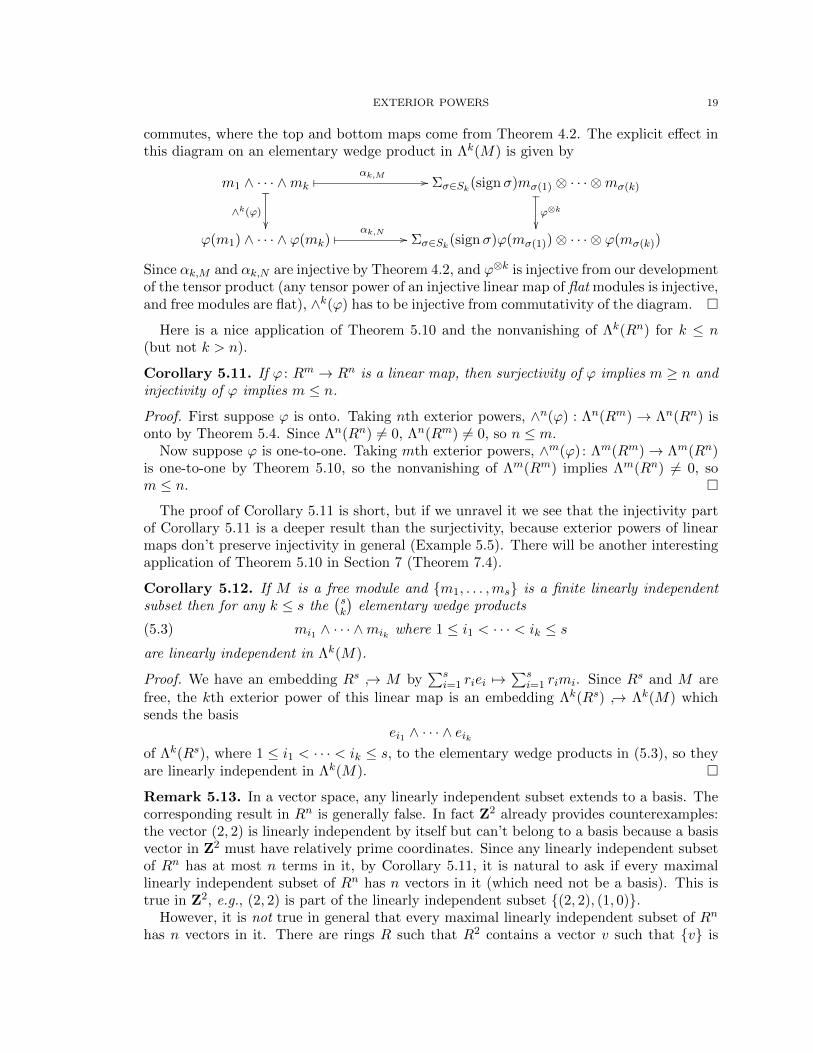
commutes, where the top and bottom maps come from Theorem 4.2. The explicit effect inthis diagram on an elementary wedge product in Λk(M) is given by

m1 ∧ · · · ∧mk� αk,M //

_

∧k(ϕ)

��

Σσ∈Sk(signσ)mσ(1) ⊗ · · · ⊗mσ(k)_

ϕ⊗k

��ϕ(m1) ∧ · · · ∧ ϕ(mk)

� αk,N // Σσ∈Sk(signσ)ϕ(mσ(1))⊗ · · · ⊗ ϕ(mσ(k))

Since αk,M and αk,N are injective by Theorem 4.2, and ϕ⊗k is injective from our developmentof the tensor product (any tensor power of an injective linear map of flat modules is injective,and free modules are flat), ∧k(ϕ) has to be injective from commutativity of the diagram. �

Here is a nice application of Theorem 5.10 and the nonvanishing of Λk(Rn) for k ≤ n(but not k > n).

Corollary 5.11. If ϕ : Rm → Rn is a linear map, then surjectivity of ϕ implies m ≥ n andinjectivity of ϕ implies m ≤ n.

Proof. First suppose ϕ is onto. Taking nth exterior powers, ∧n(ϕ) : Λn(Rm) → Λn(Rn) isonto by Theorem 5.4. Since Λn(Rn) 6= 0, Λn(Rm) 6= 0, so n ≤ m.

Now suppose ϕ is one-to-one. Taking mth exterior powers, ∧m(ϕ) : Λm(Rm)→ Λm(Rn)is one-to-one by Theorem 5.10, so the nonvanishing of Λm(Rm) implies Λm(Rn) 6= 0, som ≤ n. �

The proof of Corollary 5.11 is short, but if we unravel it we see that the injectivity partof Corollary 5.11 is a deeper result than the surjectivity, because exterior powers of linearmaps don’t preserve injectivity in general (Example 5.5). There will be another interestingapplication of Theorem 5.10 in Section 7 (Theorem 7.4).

Corollary 5.12. If M is a free module and {m1, . . . ,ms} is a finite linearly independentsubset then for any k ≤ s the

(sk

)elementary wedge products

(5.3) mi1 ∧ · · · ∧mik where 1 ≤ i1 < · · · < ik ≤ sare linearly independent in Λk(M).

Proof. We have an embedding Rs ↪→ M by∑s

i=1 riei 7→∑s

i=1 rimi. Since Rs and M are

free, the kth exterior power of this linear map is an embedding Λk(Rs) ↪→ Λk(M) whichsends the basis

ei1 ∧ · · · ∧ eikof Λk(Rs), where 1 ≤ i1 < · · · < ik ≤ s, to the elementary wedge products in (5.3), so theyare linearly independent in Λk(M). �

Remark 5.13. In a vector space, any linearly independent subset extends to a basis. Thecorresponding result in Rn is generally false. In fact Z2 already provides counterexamples:the vector (2, 2) is linearly independent by itself but can’t belong to a basis because a basisvector in Z2 must have relatively prime coordinates. Since any linearly independent subsetof Rn has at most n terms in it, by Corollary 5.11, it is natural to ask if every maximallinearly independent subset of Rn has n vectors in it (which need not be a basis). This istrue in Z2, e.g., (2, 2) is part of the linearly independent subset {(2, 2), (1, 0)}.

However, it is not true in general that every maximal linearly independent subset of Rn

has n vectors in it. There are rings R such that R2 contains a vector v such that {v} is

20 KEITH CONRAD

linearly independent (meaning it’s torsion-free) but there is no linearly independent subset{v, w} in R2. An example, due to David Speyer, is the following: let R be the ring offunctions C2 − {(0, 0)} → C which coincide with a polynomial function at all but finitelymany points. (The finitely many exceptional points can vary.) Letting z and w be thecoordinate functions on C2, in R2 the vector (z, w) is linearly independent and is not partof any larger linearly independent subset.

6. Determinants

Now we put exterior powers to work in the development of the determinant, whoseproperties have up until now played no role except for a 2× 2 determinant in Example 5.5.

Let M be a free R-module of rank d ≥ 1. The top exterior power Λd(M) is a free R-module of rank 1, so any linear map Λd(M) → Λd(M) is scaling by an element of R. Fora linear map ϕ : M → M , the induced linear map ∧d(ϕ) : Λd(M) → Λd(M) is scaling bywhat element of R?

Theorem 6.1. If M is a free R-module of rank d ≥ 1 and ϕ : M →M is a linear map, itstop exterior power ∧d(ϕ) : Λd(M)→ Λd(M) is multiplication by detϕ ∈ R.

Proof. We want to show ∧d(ϕ)(ω) = (detϕ)ω for all ω ∈ Λd(M). It suffices to check thiswhen ω is a basis of Λd(M). Let e1, . . . , ed be a basis for M , so e1 ∧ · · · ∧ ed is a basis forΛd(M). We will show

∧d(ϕ)(e1 ∧ · · · ∧ ed) = (detϕ)(e1 ∧ · · · ∧ ed).

By definition,

∧d(ϕ)(e1 ∧ · · · ∧ ed) = ϕ(e1) ∧ · · · ∧ ϕ(ed).

Let ϕ(ej) =∑d

i=1 aijei. Then (aij) is the matrix representation for ϕ in the ordered basise1, . . . , ed and

∧d(ϕ)(e1 ∧ · · · ∧ ed) =d∑i=1

ai1ei ∧ · · · ∧d∑i=1

aidei

=d∑

i1=1

ai11ei1 ∧ · · · ∧d∑

id=1

aiddeid ,

where we introduce different labels for the summation indices because we are about tocombine terms using multilinearity:

∧d(ϕ)(e1 ∧ · · · ∧ ed) =

d∑i1,...,id=1

ai11 · · · aiddei1 ∧ · · · ∧ eid .

In this sum, terms with equal indices can be dropped (the wedge product vanishes) so allwe are left with is a sum over d-tuples of distinct indices. Since d distinct integers from 1to d must be 1, 2, . . . , d in some rearrangement, we can write i1 = σ(1), . . . , id = σ(d) as σruns over Sd:

∧d(ϕ)(e1 ∧ · · · ∧ ed) =

d∑σ∈Sd

aσ(1)1 · · · aσ(d)d(eσ(1) ∧ · · · ∧ eσ(d)).

EXTERIOR POWERS 21

By (3.2), this becomes

∧d(ϕ)(e1 ∧ · · · ∧ ed) =

d∑σ∈Sd

(signσ)aσ(1)1 · · · aσ(d)d(e1 ∧ · · · ∧ ed).

Thus ∧d(ϕ) acts on the 1-element basis e1 ∧ · · · ∧ ed of Λd(M) as multiplication by thenumber we recognize as det((aij)

>) = det(aij) = det(ϕ), so it acts on every element of

Λd(M) as scaling by det(ϕ). �

Since we did not use determinants before, we could define the determinant of a linearoperator ϕ on a (nonzero) finite free module M to be the scalar by which ϕ acts on the topexterior power of M . Then the proof of Theorem 6.1 shows detϕ can be computed from anymatrix representation of ϕ by the usual formula, and it shows this formula is independentof the choice of matrix representation for ϕ since our construction of exterior powers wascoordinate-free. Since ∧k(idM ) = idΛk(M), the determinant of the identity map is 1. Hereis a slick proof that the determinant is multiplicative:

Corollary 6.2. If M is a nonzero finite free R-module and ϕ and ψ are linear mapsM →M , then det(ψ ◦ ϕ) = det(ψ) det(ϕ).

Proof. Let M have rank d ≥ 1. By Theorem 5.1, ∧d(ψ ◦ϕ) = ∧d(ψ) ◦∧d(ϕ). Both sides arelinear maps Λd(M)→ Λd(M) and Λd(M) is free of rank 1. The left side is multiplication bydet(ψ ◦ϕ). The right side is multiplication by det(ϕ) followed by multiplication by det(ψ),which is multiplication by det(ψ) det(ϕ). Thus, by checking both sides on a one-elementbasis of Λd(M), we obtain det(ψ ◦ ϕ) = det(ψ) det(ϕ). �

Continuing a purely logical development (not assuming prior knowledge of determinants,that is), at this point we could introduce the characteristic polynomial and prove the Cayley-Hamilton theorem. One of the corollaries of the Cayley-Hamilton theorem is that GLd(R) ={A ∈ Md(R) : detA ∈ R×}. That is used in the next result, which characterizes bases inRd using Λd(R).

Corollary 6.3. Let M be a free R-module of rank d ≥ 1. For x1, . . . , xd ∈M , {x1, . . . , xd}is a basis of M if and only if x1 ∧ · · · ∧ xd is a basis of Λd(M).

Proof. We know by Theorem 4.2 that if {x1, . . . , xd} is a basis of M then x1 ∧ · · · ∧ xd is abasis of Λd(M). We now want to go the other way: if x1 ∧ · · · ∧ xd is a basis of Λd(M) weshow {x1, . . . , xd} is a basis of M .

Since M is free of rank d it has some basis, say {e1, . . . , ed}. Write the xj ’s in terms ofthis basis: xj =

∑ni=1 aijej , where aij ∈ R. That means the linear map A : M → M given

by A(ej) = xj for all j has matrix representation (aij) in the basis {e1, . . . , ed}. Therefore

x1 ∧ · · · ∧ xd = Ae1 ∧ · · · ∧Aed = ∧d(A)(e1 ∧ · · · ∧ ed) = (detA)(e1 ∧ · · · ∧ ed).Since x1 ∧ · · · ∧ xd and e1 ∧ · · · ∧ ed are both bases of Λd(M) (the first by hypothesis andthe second by Theorem 4.2), the scalar by which they differ must be a unit: detA ∈ R×.Therefore A ∈ GLd(R), so the xj ’s must be a basis of Rd because A(ej) = xj and the ej ’sare a basis. �

While the top exterior power of a linear operator on a finite free module is multiplicationby its determinant, the lower-order exterior powers of a linear map between finite freemodules have matrix representations whose entries are determinants. Let ϕ : M → N be

22 KEITH CONRAD

linear, with M and N finite free of positive ranks m and n, respectively. Take k ≤ m andk ≤ n since otherwise Λk(M) or Λk(N) is 0. Pick bases e1, . . . , em for M and f1, . . . , fn forN . The corresponding basis of Λk(M) is all ej1 ∧ · · · ∧ ejk where

1 ≤ j1 < · · · < jk ≤ m,Similarly, the corresponding basis for Λk(N) is all fi1∧· · ·∧fik where 1 ≤ i1 < · · · < ik ≤ n.The matrix for ∧k(ϕ) relative to these bases of Λk(M) and Λk(N) is therefore naturallyindexed by pairs of increasing k-tuples.

Theorem 6.4. With notation as above, let [ϕ] denotes the n×m matrix for ϕ relative tothe choice of bases for M and N . Relative to the corresponding bases on Λk(M) and Λk(N),the matrix entry for ∧k(ϕ) in row position (i1, . . . , ik) and column position (j1, . . . , jk) isthe determinant of the k× k matrix built from rows i1, . . . , ik and columns j1, . . . , jk of [ϕ].

Proof. The matrix entry in question is the coefficient of fi1 ∧ · · · ∧ fik in the expansion of∧k(ϕ)(ej1 ∧ · · · ∧ ejk) = ϕ(ej1) ∧ · · · ∧ ϕ(ejk). Details are left to the reader. �

In short, this says the kth exterior power of a linear map ϕ has matrix entries which arek × k determinants of submatrices of the matrix of ϕ.

Example 6.5. In Example 5.3 we computed the second exterior power of the linear mapR3 → R3 given by the 3×3 matrix L in (5.1). The result is a matrix of size

(32

)×(

32

)= 3×3

matrix whose rows and columns are associated to basis pairs ei ∧ ei′ and ej ∧ ej′ , where theordering of the basis was e1 ∧ e2, e1 ∧ e3, and e2 ∧ e3. For instance, the upper right entry inthe matrix for ∧2(L) is in its first row and third column, so it is the e1 ∧ e2-coefficient of∧2(L)(e2 ∧ e3). This matrix entry has row position (1, 2) (index for the first basis vector)and column position (2, 3) (index for the third basis vector). The 2 × 2 submatrix of Lusing rows 1 and 2 and columns 2 and 3 is ( 2 0

1 1 ), whose determinant is 2, which matchesthe upper right entry in the matrix at the end of Example 5.3.

7. Exterior powers and linear independence

This section discusses the connection between elementary wedge products and linearindependence in a free module. We will start off with vector spaces, which are easier tohandle.

If we are given n vectors in Rn, there are two ways to determine if they are linearlyindependent using the n×n matrix with the vectors as the columns. The first way is to rowreduce the matrix and see if you get the identity matrix. The second way is to compute thedeterminant of the matrix and see if you get a nonzero value. How can we decide if a set ofk < n vectors in Rn is linearly dependent? Again there are two ways, each generalizing oneof the previous two methods in terms of the n×k matrix having the vectors as the columns.The first way is to row reduce the matrix to see if a k × k submatrix is the identity. Thesecond way is to compute the determinants of all k × k submatrices and see if any of themis not 0. Whereas the first way (row reduction) provides a set of steps that always keepsyou going in the right direction, the second way involves one determinant computation afterthe other, and that will take longer to complete (particularly if all the determinants turnout to be 0!). Using exterior powers, we can carry out all these determinant computationsat once. That is the algorithmic content of the next theorem for finite-dimensional vectorspaces, if you keep in mind how determinants are related to coefficients in wedge productexpansions.

EXTERIOR POWERS 23

Theorem 7.1. Let V be a vector space. The vectors v1, . . . , vk in V are linearly independentif and only if v1 ∧ · · · ∧ vk 6= 0 in Λk(V ).

Proof. The case k = 1 is trivial, so take k ≥ 2. First assume {v1, . . . , vk} is a linearlyindependent set. This set extends to a basis of V (we are working over a field!), so v1∧· · ·∧vkis part of a basis of Λk(V ) by Theorem 4.2. In particular, v1 ∧ · · · ∧ vk 6= 0 in Λk(V ).

Now suppose {v1, . . . , vk} is linearly dependent, so one vi is a linear combination of theothers. Whether or not v1 ∧ · · · ∧ vk is nonzero in Λk(V ) is independent of the order of thefactors, since permuting the terms only changes the elementary wedge product by a sign,so we may suppose vk is a linear combination of the rest:

vk = c1v1 + · · ·+ ck−1vk−1.

Then in Λk(V ),

v1 ∧ · · · ∧ vk−1 ∧ vk = v1 ∧ · · · ∧ vk−1 ∧

(k−1∑i=1

civi

).

Expanding the right side gives a sum of k − 1 wedge products, each containing a repeatedvector, so every term vanishes. �

In this theorem V can be an infinite-dimensional vector space since we never requiredfinite-dimensionality in the proof. At one point we invoked Theorem 4.2, which was provedfor all free modules, not just free modules with a finite basis.

Corollary 7.2. If V is a vector space and v1, . . . , vk are linearly independent in V , thenan element v ∈ V is a linear combination of v1, . . . , vk if and only if v1 ∧ · · · ∧ vk ∧ v = 0 inΛk+1(V ).

Proof. Because the vi’s are linearly independent, v is a linear combination of them if andonly if {v1, . . . , vk, v} is linearly dependent, and that is equivalent to their wedge productvanishing by Theorem 7.1. �

Example 7.3. In R3, does the vector v = (4,−1, 1) lie in the span of v1 = (2, 1, 3) andv2 = (1, 2, 4)? Since v1 and v2 are linearly independent, v is in their span if and only ifv1∧ v2∧ v vanishes in Λ3(R3). Let e1, e2, e3 be the standard basis of R3. Then we compute

v1 ∧ v2 = (2e1 + e2 + 3e3) ∧ (e1 + 2e2 + 4e3)

= 4(e1 ∧ e2) + 8(e1 ∧ e3)− e1 ∧ e2 + 4(e2 ∧ e3)

−3(e1 ∧ e3)− 6(e2 ∧ e3)

= 3(e1 ∧ e2) + 5(e1 ∧ e3)− 2(e2 ∧ e3)

so

v1 ∧ v2 ∧ v = (3(e1 ∧ e2) + 5(e1 ∧ e3)− 2(e2 ∧ e3)) ∧ (4e1 − e2 + e3)

= 3(e1 ∧ e2 ∧ e3)− 5(e1 ∧ e3 ∧ e2)− 8(e2 ∧ e3 ∧ e1)

= 3(e1 ∧ e2 ∧ e3) + 5(e1 ∧ e2 ∧ e3)− 8(e1 ∧ e2 ∧ e3)

= 0.

Since this vanishes, (4,−1, 1) is in the span of (2, 1, 3) and (1, 2, 4).This method does not explicitly represent (4,−1, 1) as a linear combination in the span

of (2, 1, 3) and (1, 2, 4). (Here is one: (4,−1, 1) = 3(2, 1, 3)− 2(1, 2, 4).) On the other hand,if we are only concerned with an existence question (is it in the span, not how is it in the

24 KEITH CONRAD

span) then this procedure works just as the computation of a determinant does to detectinvertibility of a matrix without providing a formula for the inverse matrix.

There is a generalization of Theorem 7.1 to describe linear independence in a free R-module M rather than in a vector space. Given m1, . . . ,mk in M , their linear independenceis equivalent to a property ofm1∧· · ·∧mk in Λk(M), but the property is not the nonvanishingof this elementary wedge product:

Theorem 7.4. Let M be a free R-module. Elements m1, . . . ,mk in M are linearly indepen-dent in M if and only if m1∧· · ·∧mk in Λk(M) is torsion-free: for r ∈ R, r(m1∧· · ·∧mk) = 0only when r = 0.

When R is a field, we recover Theorem 7.1. What makes Theorem 7.4 more subtle thanTheorem 7.1 is that a linearly independent set in a free module usually does not extend toa basis, so we can’t blindly adapt the proof of Theorem 7.1 to the case of free modules.

Proof. The case k = 1 is trivial by the definition of a linearly independent set in a module,so we can take k ≥ 2.

Assume m1, . . . ,mk is a linearly independent set in M . By Corollary 5.12, the elementarywedge product m1 ∧ · · · ∧ mk is a linearly independent one-element subset in Λk(M), som1 ∧ · · · ∧mk has no R-torsion.

If the mi’s are linearly dependent, say r1m1 + · · · + rkmk = 0 with ri ∈ R not all 0, wemay re-index and assume r1 6= 0. Then

0 = (r1m1 + · · ·+ rkmk) ∧m2 ∧ · · · ∧mk = r1(m1 ∧m2 ∧ · · · ∧mk),

so m1 ∧m2 ∧ · · · ∧mk has R-torsion. �

Corollary 7.5. A system of d equations in d unknowns

a11x1 + · · ·+ a1dxd = 0

a21x1 + · · ·+ a2dxd = 0...

ad1x1 + · · ·+ addxd = 0

in a commutative ring R has a nonzero solution x1, . . . , xd ∈ R if and only if det(aij) is azero divisor in R.

Proof. We rewrite the theorem in terms of matrices: for A ∈ Md(R), the equation Av = 0has a nonzero solution v ∈ Rd if and only if detA is a zero divisor in R.

We consider the negated property, that the only solution of Av = 0 is v = 0. This isequivalent to the columns of A being linearly independent. The columns are Ae1, . . . , Aed,and their elementary wedge product is

Ae1 ∧ · · · ∧Aed = (detA)e1 ∧ · · · ∧ ed ∈ Λd(Rd).

Since e1 ∧ · · · ∧ ed is a basis of Λd(Rd) as an R-module, (detA)e1 ∧ · · · ∧ ed is torsion-free ifand only if the only solution of r detA = 0 is r = 0, which means detA is not a zero divisor.Thus Av = 0 has a nonzero solution if and only if detA is a zero divisor. �

We can turn Theorem 7.4 into a characterization of linear independence of k vectorsv1, . . . , vk in Rd when k ≤ d.3 The test is that v1 ∧ · · · ∧ vk is torsion-free in Λk(Rd). If we

3We may as well let k ≤ d, since a linearly independent subset of Rd has at most d terms by Corollary5.11.

EXTERIOR POWERS 25

let A ∈ Md×k(R) be the matrix whose columns are v1, . . . , vk, linear independence of thecolumns is the same thing as injectivity of A as a linear map Rk → Rd. So we can now say,for k ≤ d, when a matrix in Md×k(R) is injective as a linear transformation: if and onlyif the elementary wedge product of its columns is torsion-free in Λk(Rd). What does that

mean concretely? Writing vj =∑d

i=1 aijei using the standard basis e1, . . . , ed of Rd,

v1 ∧ · · · ∧ vk =∑

1≤i1<···<ik≤d

∣∣∣∣∣∣∣a1i1 · · · a1ik

.... . .

...aki1 · · · akik

∣∣∣∣∣∣∣ ei1 ∧ · · · ∧ eik .This is torsion-free precisely when the coefficients are not all killed by a common nonzeroelement of R. Therefore we get the rule: for k ≤ d, A ∈ Md×k(R) is injective as a linearmap Rk → Rd if and only if the determinants of its k × k submatrices have no commonnonzero annihilator in R.

Example 7.6. Let

A =

2 21 51 2

∈ M3×2(Z/6Z).

Its 2 × 2 submatrices have determinants 8,−3, 2, which equal 2, 3, 2 in Z/6Z. Althoughnone of these determinants is a unit in Z/6Z, which would be an easy way to see injectivity,A is still injective because 2 and 3 have no common nonzero annihilator in Z/6Z (that is,2r = 0 and 3r = 0 only for r = 0). In the terminology of linear independence, we showedthe two columns of A are linearly independent in (Z/6Z)3. (This does not mean neithercolumn is a scalar multiple of the other, but it means the stronger assertion that no linearcombination of the columns is 0 except for the trivial combination with both coefficientsequal to 0.)

We can also check this in Λ2((Z/6Z)3): the two columns of A are 2e1 + e2 + e3 and2e1 + 5e2 + 2e3, and

(2e1 + e2 + e3) ∧ (2e1 + 5e2 + 2e3) = 2e1 ∧ e2 + 2e1 ∧ e3 + 3e2 ∧ e3,

which is torsion-free since 2r = 0 and 3r = 0 in Z/6Z only for r = 0.That the coefficients in the elementary wedge product match the determinants of the

2× 2 submatrices illustrates that the rules about elementary wedge product computationsreally do encode everything about determinants of submatrices.

I learned the following neat use of Corollary 7.5 from [2, pp. 6–7].

Theorem 7.7. Let M be an R-module admitting a linear injection Rd ↪→ M and a linearsurjection Rd �M . Then M ∼= Rd.

Proof. The hypotheses say M has a d-element spanning set and a d-element linearly inde-pendent subset. Call the former x1, . . . , xd and the latter e1, . . . , ed, so we can write

M = Rx1 + · · ·+Rxd, ei =d∑j=1

aijxj .

The xj ’s span M . We want to show they are linearly independent, so they form a basis andM is free of rank d.

26 KEITH CONRAD

The expression of the ei’s in terms of the xj ’s can be written as the vector-matrix equation

(7.1)

e1...ed

= (aij)

x1...xd

,

where we treat (aij) ∈ Md(R) as a matrix acting on the d-tuples in Md.We show by contradiction that ∆ := det(aij) is not a zero divisor in R. If ∆ is a zero

divisor then the columns of (aij) are linearly dependent by Corollary 7.5. A square matrixand its transpose have the same determinant, so the rows of (aij) are also linearly dependent.That means there are c1, . . . , cd ∈ R not all 0 such that

(c1, . . . , cd)(aij) = (0, . . . , 0).

Using this, we multiply both sides of (7.1) on the left by (c1, . . . , cd) to get

(c1, . . . , cd)

e1...ed

= 0.

That says c1e1 + · · ·+ cded = 0, which contradicts linear independence of the ei’s. So ∆ isnot a zero divisor.

Suppose now that a1x1 + · · ·+ adxd = 0. We want to show every ai is 0. Multiply bothsides of (7.1) on the left by the cofactor matrix for (aij) (that’s the matrix you multiply byto get the scalar diagonal matrix with the determinant ∆ along the main diagonal):

cof(aij)

e1...ed

= ∆

x1...xd

.

Now multiply both sides of this equation on the left by (a1, . . . , ad):

(a1, . . . , ad) cof(aij)

e1...ed

= ∆(a1x1 + · · ·+ adxd) = 0.

The product (a1, . . . , ad) cof(aij) is a (row) vector, say (b1, . . . , bd). Then b1e1+· · ·+bded = 0,so every bi is 0 by linear independence of the ei’s. Therefore (a1, . . . , ad) cof(aij) = (0, . . . , 0).Multiply both sides of this on the right by (aij) to get (a1, . . . , ad)∆ = (0, . . . , 0), so ∆ai = 0for all i. Since ∆ is not a zero divisor, every ai is 0 and we are done. �

8. The wedge product

By concatenating elementary wedge products, we introduce a multiplication operationbetween different exterior powers of a module.

Lemma 8.1. If f : M × · · · ×M︸ ︷︷ ︸k times

×N1 · · ·×N` is multilinear and is alternating in the M ’s,

there is a unique multilinear map f̃ : Λk(M)×N1 × · · · ×N` → N such that

f̃(m1 ∧ · · · ∧mk, n1, . . . , n`) = f(m1, . . . ,mk, n1, . . . , n`).

EXTERIOR POWERS 27

Proof. Uniqueness of f̃ follows from multilinearity. To prove existence of f̃ , fix a choice ofn1 ∈ N1, . . . , n` ∈ N`. Define fn1,...,n` : Mk → N by

fn1,...,n`(m1, . . . ,mk) = f(m1, . . . ,mk, n1, . . . , n`).

Since f is multilinear, fn1,...,n` is multilinear. Since f is alternating in the mi’s, fn1,...,n` is

an alternating map. Therefore there is a unique linear map f̃n1,...,n` : Λk(M)→ N such that

f̃n1,...,n`(m1 ∧ · · · ∧mk) = fn1,...,n`(m1, . . . ,mk) = f(m1, . . . ,mk, n1, . . . , n`).

on elementary wedge products.

Define f̃ : Λk(M) × N1 × · · · × N` → N by f̃(ω, n1, . . . , n`) = fn1,...,n`(ω). Since each

fn1,...,n` is linear, f̃ is linear in its first component. To check f̃ is linear in one of its othercoordinates, we carry it out for n1 (all the rest are similar). We want to verify that

f̃(ω, n1 + n′1, n2, . . . , n`) = f̃(ω, n1, n2, . . . , n`) + f̃(ω, n′1, n2, . . . , n`)

and

f̃(ω, rn1, n2, . . . , n`) = rf̃(ω, n1, n2, . . . , n`).

Both sides of both equations are additive in ω, so it suffices to check the identity whenω = m1 ∧ · · · ∧mk is an elementary wedge product. In that case the two equations turninto linearity of f in its N1-component, and that is just a special case of the multilinearityof f . �

Theorem 8.2. Let M be an R-module. For positive integers k and `, there is a uniqueR-bilinear map Λk(M)× Λ`(M)→ Λk+`(M) satisfying the rule

(m1 ∧ · · · ∧mk,m′1 ∧ · · · ∧m′`) 7→ m1 ∧ · · · ∧mk ∧m′1 ∧ · · · ∧m′`

on pairs of elementary wedge products.

Proof. Since the elementary wedge products span each exterior power module, and a bilinearmap is determined by its values on pairs coming from spanning sets, there is at most onebilinear map with the prescribed behavior. As usual in this game, what needs proof is theexistence of such a map.

Start by backing up and considering the function f : Mk ×M ` → Λk+`(M) by

f(m1, . . . ,mk,m′1, . . . ,m

′`) = m1 ∧ · · · ∧mk ∧m′1 ∧ · · · ∧m′`.

This is multilinear and alternating in the first k-coordinates, so by Lemma 8.1 there is a

multilinear map f̃ : Λk(M)×M ` → Λk+`(M) such that

f̃(m1 ∧ · · · ∧mk,m′1, . . . ,m

′`) = m1 ∧ · · · ∧mk ∧m′1 ∧ · · · ∧m′`.

and it is alternating in its last ` coordinates. Therefore, again by Lemma 8.1, there is abilinear map B : Λk(M)× Λ`(M)→ Λk+`(M) such that

B(ω,m′1 ∧ · · ·m′`) = f̃(ω,m′1, . . . ,m′`),

so

B(m1 ∧ · · · ∧mk,m′1 ∧ · · ·m′`) = f̃(m1 ∧ · · · ∧mk,m

′1, . . . ,m

′`)

= m1 ∧ · · · ∧mk ∧m′1 ∧ · · · ∧m′`.We have produced a bilinear map on the kth and `th exterior powers with the desired valueon pairs of elementary wedge products. �

28 KEITH CONRAD

The operation constructed in Theorem 8.2, sending Λk(M) × Λ`(M) to Λk+`(M), isdenoted ∧ and is called the wedge product. We place the operation in between the elementsit acts on, just like other multiplication functions in mathematics. So for any ω ∈ Λk(M)and η ∈ Λ`(M) we have an element ω ∧ η ∈ Λk+`(M), and this operation is bilinear in ωand η. The formula in Theorem 8.2 on two elementary wedge products looks like this:

(m1 ∧ · · · ∧mk) ∧ (m′1 ∧ · · · ∧m′`) = m1 ∧ · · ·mk ∧m′1 ∧ · · · ∧m′`.

Notice we have given a new meaning to the notation ∧ and to the terminology “wedge prod-uct,” which we have until now used in a purely formal way always in the phrase “elementarywedge product.” This new operational meaning of the wedge product is consistent with theold formal one, e.g. the (new) wedge product operation ∧ : Λ1(M)×Λ1(M)→ Λ2(M) sends(m,m′) to m ∧m′ (old notation). This is very much like the definition of R[T ] as formalfinite sums

∑i aiT

i where, after the ring operations are defined, the symbol T i is recognizedas the i-fold product of the element T .

We have defined a wedge product Λk(M)×Λ`(M)→ Λk+`(M) when k and ` are positive.What if one of them is 0? Recall (by definition) Λ0(M) = R. Theorem 8.2 extends to thecase k = 0 or ` = 0 if we let the maps Λ0(M)× Λ`(M) → Λ`(M) and Λk(M)× Λ0(M) →Λ0(M) be scalar multiplication: r ∧ η = rη and ω ∧ r = rω.

Now we can think about the old notation m1 ∧ · · · ∧ mk in an operational way: it isthe result of applying the wedge product operation k times with elements from the moduleΛ1(M) = M . Since we are now able to speak about a wedge product ω1∧· · ·∧ωk where theωi’s lie in exterior power modules Λki(M), the elementary wedge products m1 ∧ · · · ∧mk,where the factors are in M , are merely special cases of wedge products.

Actually, to speak of ω1 ∧ · · · ∧ ωk unambiguously we need ∧ to be associative! So let’scheck that.

Theorem 8.3. The wedge product is associative: if ω ∈ Λa(M), η ∈ Λb(M), and ξ ∈ Λc(M)then (ω ∧ η) ∧ ξ = ω ∧ (η ∧ ξ) in Λa+b+c(M).

Proof. This is easy if a, b, or c is zero (then one of ω, η, and ξ is in R, and wedging with Ris just scalar multiplication), so we can assume a, b, and c are all positive.

Let f and g be the functions from Λa(M)×Λb(M)×Λc(M) to Λa+b+c(M) given by bothchoices of parentheses:

f(ω, η, ξ) = (ω ∧ η) ∧ ξ, g(ω, η, ξ) = ω ∧ (η ∧ ξ).

(Note ω∧η ∈ Λa+b(M) and η∧ξ ∈ Λb+c(M).) Since the wedge product on two exterior powermodules is bilinear, f and g are both trilinear functions. Therefore to show f = g it sufficesto verify equality on triples of elementary wedge products, since they are spanning sets ofΛa(M), Λb(M), and Λc(M). On such elements the equality is obvious by the definition ofthe wedge product operation, so we are done. �

The following theorem puts associativity of the wedge product to work.

Theorem 8.4. Let M be an R-module. If some Λi(M) is finitely generated, then Λj(M)is finitely generated for all j ≥ i.

EXTERIOR POWERS 29

The important point here is that we are not assuming M is finitely generated, onlythat some exterior power is finitely generated. Because exterior powers are not definedrecursively, this theorem is not a tautology.4

Proof. It suffices to show that if Λi(M) is finitely generated then Λi+1(M) is finitely gener-ated. Our argument is a simplification of [3, Lemma 2.1].

The module Λi(M) has a finite spanning set, which we can take to be a set of elementarywedge products. Let x1, . . . , xp ∈ M be the terms appearing in those elementary wedgeproducts, so Λi(M) is spanned by the i-fold wedges of x1, . . . , xp.

We will show Λi+1(M) is spanned by the (i + 1)-fold wedges of x1, . . . , xp. It sufficesto show the span of these wedges contains all the elementary wedge products in Λi+1(M).Choose (i+ 1)-fold elementary wedge product, say

y1 ∧ · · · ∧ yi ∧ yi+1 = (y1 ∧ · · · ∧ yi) ∧ yi+1.

Since y1 ∧ · · · ∧ yi is in Λi(M), it is an R-linear combination of i-fold wedges of x1, . . . , xp.Therefore y1 ∧ · · · ∧ yi ∧ yi+1 is an R-linear combination of expressions

(xj1 ∧ · · · ∧ xji) ∧ yi+1 = xj1 ∧ (xj2 ∧ · · · ∧ xji ∧ yi+1),

where the equation uses associativity of the wedge product. Since xj2 ∧ · · · ∧ xji ∧ yi+1 is inΛi(M), it is an R-linear combination of i-fold wedges of x1, . . . , xp. �

Theorem 8.5. If M is spanned as an R-module by x1, . . . , xd then for 1 ≤ k ≤ d everyelement of Λk(M) is a sum

ω1 ∧ x1 + ω2 ∧ x2 + · · ·+ ωd ∧ xdfor some ωi ∈ Λk−1(M).

We don’t consider k > d in this theorem since Λk(M) = 0 for such k by Theorem 4.1.

Proof. The result is clear when k = 1 since Λ0(M) = R by definition, so we can assumek ≥ 2. From the beginning of Section 4, Λk(M) is spanned as an R-module by the k-foldelementary wedge products xi1 ∧ · · · ∧ xik where 1 ≤ i1 < · · · < ik ≤ d. Using the wedgeproduct multiplication Λk−1(M)×M → Λk(M), we can write

xi1 ∧ · · · ∧ xik = η ∧ xik ,

where η = xi1 ∧ · · · ∧ xik−1∈ Λk−1(M). Therefore every element of Λk(M) is an R-linear

combination r1(η1 ∧ x1) + · · · + rd(ηd ∧ xd), where ri ∈ R and ηi ∈ Λk−1(M). Sinceri(ηi ∧ xi) = (riηi) ∧ xi we can set ωi = riηi and we’re done. �

Here is an analogue of Theorem 4.8 for linear maps.

Theorem 8.6. Let ϕ : M → N be a linear map of R-modules. If ∧i(ϕ) = 0 for some i then∧j(ϕ) = 0 for all j ≥ i.

Theorem 4.8 is the special case when N = M and ϕ = idM (why?).

4The theorem doesn’t go backwards down to M , i.e., if some Λi(M) is finitely generated this does notimply M is finitely generated. For example, Λ2(Q/Z) = 0 as a Z-module, but Q/Z is not finitely generatedas a Z-module.

30 KEITH CONRAD

Proof. It suffices so show ∧i+1(ϕ) = 0.Since ∧i(ϕ) = 0 for any m1, . . . ,mi in M we have

0 = ∧i(ϕ)(m1 ∧ · · · ∧mi) = ϕ(m1) ∧ · · · ∧ ϕ(mi)

in Λi(N). For any m1, . . . ,mi+1 in M , in Λi+1(N) we have

∧i+1(ϕ)(m1 ∧ · · · ∧mi ∧mi+1) = ϕ(m1) ∧ · · · ∧ ϕ(mi) ∧ ϕ(mi+1)

= (ϕ(m1) ∧ · · · ∧ ϕ(mi)) ∧ ϕ(mi+1)

= 0 ∧ ϕ(mi+1)

= 0.

Such terms span the image of ∧i+1(ϕ), so ∧i+1(ϕ) = 0. �

In an elementary wedge product m1 ∧ · · · ∧mk, where the factors are in M = Λ1(M),transposing two of them introduces a sign change. What is the sign-change rule for trans-posing factors in a wedge product ω1∧· · ·∧ωk? By associativity, we just need to understandhow a single wedge product ω ∧ η changes when the factors are reversed.

Theorem 8.7. For ω ∈ Λk(M) and η ∈ Λ`(M), ω ∧ η = (−1)k`η ∧ ω.

Proof. This is trivial if k = 0 or ` = 0 (in which case the wedge product is simply scalingand (−1)k` = 1), so we can take k and ` positive.

Both sides of the desired equation are bilinear functions of ω and η, so to verify equalityfor all ω and η it suffices to do so on spanning sets of the modules. Thus we can takeω = m1 ∧ · · · ∧mk and η = m′1 ∧ · · · ∧m′`, so we want to show

(8.1) m1 ∧ · · · ∧mk ∧m′1 ∧ · · · ∧m′` = (−1)k`(m′1 ∧ · · · ∧m′` ∧m1 ∧ · · · ∧mk).

Starting with the expression on the left, we successively move m′1,m′2, . . . ,m

′` to the front.

First move m′1 past each of the mi’s, which is a total of k swaps, so

m1 ∧ · · · ∧mk ∧m′1 ∧ · · · ∧m′` = (−1)km′1 ∧m1 ∧ · · · ∧mk ∧m′2 ∧ · · · ∧m′`.

Now move m′2 past every mi, introducing another set of k sign changes:

m1 ∧ · · · ∧mk ∧m′1 ∧ · · · ∧m′` = (−1)2km′1 ∧m′2 ∧m1 ∧ · · · ∧mk ∧m′3 ∧ · · · ∧m′`.

Repeat until m′` has been moved past every mi. In all, there are k` swaps, so the overall

sign at the end is (−1)k`. �

Theorem 8.8. For odd k and ω ∈ Λk(M), ω ∧ ω = 0.

Proof. There is a quick proof using Theorem 8.7 when 2 ∈ R×: ω ∧ ω = (−1)k2(ω ∧ ω) =

−(ω ∧ ω), so 2(ω ∧ ω) = 0, so ω ∧ ω = 0.To handle the general case when 2 may not be a unit, write

ω =∑i1,...,ik

ci1,...,ikmi1 ∧ · · · ∧mik =∑I

cIωI ,

where I = (i1, . . . , ik) is a multi-index of k integers and ωI = ω(i1,...,ik) is an abbreviationfor mi1 ∧ · · · ∧mik . Then, by the bilinearity of the wedge product,

(8.2) ω ∧ ω =∑I

cImI ∧∑J

cJωJ =∑I,J

cIcJωI ∧ ωJ ,

EXTERIOR POWERS 31

where I and J run over the same set of multi-indices. Note each ωI ∧ ωJ is an elementarywedge product with 2k factors.

The multi-indices I and J could be equal. In that case ωI ∧ ωJ = 0 since it is a 2k-foldelementary wedge product with repeated factors. When I 6= J the double sum in (8.2)contains

cIcJωI ∧ ωJ + cJcIωJ ∧ ωI = cIcJ(ωI ∧ ωJ + ωJ ∧ ωI).

Since ωI and ωJ are in Λk(M), ωJ ∧ωI = (−1)k2(ωI ∧ωJ) = −(ωI ∧ωJ), so cIcJ(ωI ∧ωJ +

ωJ ∧ ωI) = 0. �

What about Theorem 8.8 when k is even? If ω = m1 ∧ · · · ∧mk is an elementary wedgeproduct in Λk(M) then ω ∧ ω vanishes since it is an elementary wedge product with arepeated factor from M . But it is not generally true that ω ∧ ω = 0 for all ω ∈ Λk(M).

Example 8.9. For k ≥ 2, let M be finite free with linearly independent subset e1, . . . , e2k.Set ω = e1 ∧ · · · ∧ ek + ek+1 ∧ · · · ∧ e2k ∈ Λk(M). This is a sum of two elementary wedgeproducts, and

ω ∧ ω = 2e1 ∧ · · · ∧ ek ∧ ek+1 ∧ · · · ∧ e2k ∈ Λ2k(M).

By Corollary 5.12 and Theorem 7.4, e1 ∧ · · · ∧ ek ∧ ek+1 ∧ · · · ∧ e2k is torsion-free in Λ2k(M),so when 2 6= 0 in R we have ω ∧ ω 6= 0. Elementary wedge products always “square” to 0,so ω is not an elementary wedge product when 2 6= 0 in R.

To get practice computing in an exterior power module, we look at the equation v∧ω = 0in Λk+1(V ), where V is a vector space and ω ∈ Λk(V ).

Theorem 8.10. Let V be a vector space. For nonzero ω ∈ Λk(V ),

dim({v ∈ V : v ∧ ω = 0}) ≤ k,

with equality if and only if ω is an elementary wedge product.

Proof. The result is obvious if k = 0, so we can suppose k ≥ 1. Let v1, . . . , vd be linearlyindependent vectors in V that each wedge ω to 0. We want to show d ≤ k. Since V mightbe infinite-dimensional, we first create a suitable finite-dimensional subspace W in whichwe can work. (If you want to assume V is finite-dimensional, set W = V and skip the restof this paragraph.) Let W be the span of v1, . . . , vd and the nonzero vectors appearing insome fixed representation of ω as a finite sum of elementary wedge products in Λk(V ). ThenW is finite-dimensional. There’s a natural embedding W ↪→ V and we get an embeddingΛ`(W ) ↪→ Λ`(V ) in a natural way for all ` by Corollary 5.9. If we view each vi in W and ωin Λk(W ) then the condition vi ∧ ω = 0 in Λk+1(V ) implies vi ∧ ω = 0 in Λk+1(W ).

Set n = dimW , so obviously d ≤ n. If k ≥ n then obviously d ≤ k, so we can supposek ≤ n− 1.

Extend {v1, . . . , vd} to a basis {v1, . . . , vn} of W . Using this basis we can write ω inΛk(W ) as a finite sum of linearly independent elementary wedge products:

ω =∑

1≤i1<···<ik≤nci1,...,ikvi1 ∧ · · · ∧ vik

32 KEITH CONRAD

and some coefficient is not 0. Fix i between 1 and d, and compute vi∧ω using this formula:

0 = vi ∧ ω=

∑1≤i1<···<ik≤n

ci1,...,ikvi ∧ vi1 ∧ · · · ∧ vik

=∑

1≤i1<···<ik≤ni1,...,ik 6=i

ci1,...,ikvi ∧ vi1 ∧ · · · ∧ vik .

This equation is taking place in Λk+1(W ), where the (k + 1)-fold wedges vi ∧ vi1 ∧ · · · ∧ vikfor i 6∈ {i1, . . . , ik} are linearly independent. Therefore the coefficients here are all 0:

i 6∈ {i1, . . . , ik} ⇒ ci1,...,ik = 0.

Here i was any number from 1 to d, so

ci1,...,ik 6= 0⇒ {1, . . . , d} ⊂ {i1, . . . , ik}.

There is at least one nonzero coefficient, so we must have {1, . . . , d} ⊂ {i1, . . . , ik} for somek-tuple of indices. Counting the two sets, d ≤ k.

If d = k then {1, . . . , k} = {i1, . . . , ik}, which allows just one nonzero term and ω =c1,...,kv1 ∧ · · · ∧ vk, which is an elementary wedge product. Conversely, if ω is a nonzero

elementary wedge product in Λk(V ) then {v ∈ V : ω∧ v = 0} has dimension k by Corollary7.2 and associativity of the wedge product. �

Theorem 8.11. Let V be a vector space and k ≥ 1. For nonzero v ∈ V and ω ∈ Λk(V ),v ∧ ω = 0 if and only if ω = v ∧ η for some η ∈ Λk−1(V ).

Proof. By associativity, if ω = v ∧ η then v ∧ω = v ∧ (v ∧ η) = (v ∧ v)∧ η = 0. The point ofthe theorem is that the converse direction holds: if v ∧ ω = 0 then we can write ω = v ∧ ηfor some η.

As in the proof of the previous theorem, we can reduce to the finite-dimensional case(details left to the reader), so we’ll just take V to be a finite-dimensional vector space. Setn = dimV ≥ 1. Since ω ∈ Λk(V ), if k > n then ω = 0 and we can trivially write ω = v ∧ 0.So we may suppose k ≤ n. If k = 0 then ω ∈ Λ0(V ) is a scalar and wedging with ω is scalarmultiplication, so the conditions v 6= 0 and v ∧ ω = 0 imply ω = 0. Thus again ω = v ∧ 0.

Now suppose 1 ≤ k ≤ n. Extend v to a basis of V , say v1, . . . , vn where v = v1. If k = nthe condition v ∧ ω = 0 is automatic since Λn+1(V ) = 0. And it is also automatic that ωis “divisible” by v if k = n: Λn(V ) has basis v1 ∧ · · · ∧ vn, so ω = c(v1 ∧ · · · ∧ vn) for somescalar c. Then ω = v ∧ η where η = cv2 ∧ · · · ∧ vn.

We now assume 1 ≤ k ≤ n − 1 (so n ≥ 2). Using the basis of Λk(V ) coming from ourchosen basis of V that includes v as the first member v1,

(8.3) ω =∑

1≤i1<···<ik≤nci1,...,ikvi1 ∧ · · · ∧ vik

with scalar coefficients. Since v1 = v, v ∧ v1 = 0 so

(8.4) v ∧ ω =∑

2≤i1<···<ik≤nci1,...,ikv ∧ vi1 ∧ · · · ∧ vik .

The elementary wedge products on the right are part of a basis of Λk+1(V ), so from v∧ω = 0we see all the coefficients in (8.4) vanish. Thus in (8.3) the only nonzero terms are among

EXTERIOR POWERS 33

those with i1 = 1, so we can pull out v1 = v:

ω = v ∧∑

1<i2<···<ik≤nc1,i2,...,ikvi2 ∧ · · · ∧ vik .

Let η be the large sum here, so ω = v ∧ η. �

9. The exterior algebra

Since wedge products move elements into higher-degree exterior powers, we can view ∧ asmultiplication in a noncommutative ring by taking the direct sum of all the exterior powersof a module.

Definition 9.1. For an R-module M , its exterior algebra is the direct sum

Λ(M) =⊕k≥0

Λk(M) = R⊕M ⊕ Λ2(M)⊕ Λ3(M)⊕ · · · ,

provided with the multiplication rule given by the wedge product from Theorem 8.2, ex-tended distributively to the whole direct sum.

Each Λk(M) is only an R-module, but their direct sum Λ(M) is an R-algebra: it has amultiplication which commutes with scaling by R and has identity (1, 0, 0, . . . ). Notice Ris a subring of Λ(M), embedded as r 7→ (r, 0, 0, . . . ).

When Λk(M) is viewed in the exterior algebra Λ(M), it is called a homogeneous partand its elements are said to be the homogeneous terms of degree k in Λ(M). For instance,when m0, m1, m2, m3, and m4 are in M the sum m0 + m1 ∧ m2 + m3 ∧ m4 in Λ(M)has homogeneous parts m0 and m1 ∧ m2 + m3 ∧ m4. This is the same terminology usedfor homogeneous multivariable polynomials, e.g., X2 − XY + Y 3 has homogeneous partsX2 −XY (of degree 2) and Y 3 (of degree 3).

The wedge product on the exterior algebra Λ(M) is bilinear, associative, and distributive,but not commutative (unless −1 = 1 in R). The replacement for commutativity in Theorem8.7 does not generalize to a rule between all elements of Λ(M). However, if ω ∈ Λk(M) andk is even then ω commutes with every element of Λ(M), so more generally the submodule⊕

k even Λk(M) lies in the center of Λ(M).A typical element of Λ(M) is a sequence (ωk)k≥0 with ωk = 0 for k � 0, and we write

it as a formal sum∑

k≥0 ωk while keeping the direct sum aspect in mind. In this notation,

the wedge product of two elements of Λ(M) is

∑k≥0

ωk ∧∑`≥0

η` =∑p≥0

∑k+`=p

ωk ∧ η`

,

where the inner sum on the right is actual addition in Λp(M) and the outer sum is purelyformal (corresponding to the direct sum decomposition defining Λ(M)). This extensionof the wedge product from operations Λk(M) × Λ`(M) → Λk+`(M) on different exteriorpower modules to a single operation Λ(M) × Λ(M) → Λ(M) is analogous to the way themultiplication rule (aT i)(bT j) = abT i+j on monomials, which is associative, can be extendedto the usual multiplication between any two polynomials in R[T ] =

⊕i≥0RT

i. When M

is a finitely generated R-module with n generators, every Λk(M) is finitely generated as anR-module and Λk(M) = 0 for k > n so Λ(M) =

⊕nk=0 Λk(M) is finitely generated as an

R-module. Because Λk(M) is spanned as an R-module by the elementary wedge products,

34 KEITH CONRAD

and an elementary wedge product is a wedge product of elements of M , Λ(M) is generatedas an R-algebra (not as an R-module!) by M .

Theorem 9.2. When M is a free R-module of rank d, its exterior algebra is a free R-moduleof rank 2d.

Proof. Each exterior power module Λk(M) is free with rank(dk

)for 0 ≤ k ≤ d and vanishes

for k > d, so their direct sum Λ(M) is free with rank

d∑k=0

(d

k

)= 2d.

�

Concretely, when M is free with basis e1, . . . , ed, we can think of Λ(M) as an R-algebragenerated by the ei’s subject to the relations e2

i = 0 and eiej = −ejei for i 6= j. Theconstruction of Λ(M) was basis-free, but this explicit description when there is a basis ishelpful when doing computations.

Example 9.3. Let V be a real vector space of dimension 3 with basis e1, e2, e3. ThenΛ0(V ) = R, Λ1(V ) = V = Re1⊕Re2⊕Re3, Λ2(V ) = R(e1 ∧ e2)⊕R(e1 ∧ e3)⊕R(e2 ∧ e3),and Λ3(V ) = R(e1 ∧ e2 ∧ e3). The exterior algebra Λ(V ) is the direct sum of these vectorspaces and we can count the dimension as 1 + 3 + 3 + 1 = 8.

To get practice computing in an exterior algebra, we ask which elements of the exterioralgebra of a vector space wedge a given vector to 0.

Theorem 9.4. Let V be a vector space over the field K. For nonzero v ∈ V and ω ∈ Λ(V ),v ∧ ω = 0 if and only if ω = v ∧ η for some η ∈ Λ(V ).

Proof. The reduction to the case of finite-dimensional V proceeds as in the reduction stepof the proof of Theorem 8.11. By associativity, if ω = v ∧ η then v ∧ ω = v ∧ (v ∧ η) =(v ∧ v) ∧ η = 0. The point of the theorem is that the converse direction holds. First wereduce to the finite-dimensional case. Let W be the span of v and all the nonzero elementarywedge products in an expression for ω. Since W ↪→ V , Λk(W ) ↪→ Λk(V ), so Λ(W ) ↪→ Λ(V ).From these embeddings, it suffices to prove the theorem with V replaced by W , so we mayassume V is finite-dimensional.

Write ω =∑n

k=0 ωk where ωk ∈ Λk(V ) is the degree k part of ω. (If you think aboutdirect sums as sequences, ω = (ω0, . . . , ωn).) Then

v ∧ ω =n∑k=0

v ∧ ωk.

Since v ∧ ωk ∈ Λk+1(V ), the terms in the sum are in different homogeneous parts of Λ(V ),so the vanishing of v ∧ ω implies v ∧ ωk = 0 for each k. By Theorem 8.11, ω0 = 0 andfor k ≥ 1 we have ωk = v ∧ ηk−1 for some ηk−1 ∈ Λk−1(V ). Thus ω = v ∧ η whereη =

∑nk=1 ηk−1 ∈ Λ(V ). �

While we created the exterior algebra Λ(M) as a direct sum of R-modules with a snazzymultiplicative structure, it can be characterized on its own terms among R-algebras bya universal mapping property. Since each Λk(M) is spanned as an R-module by the ele-mentary wedge products m1 ∧ · · · ∧mk, Λ(M) is generated as an R-algebra (using wedge

EXTERIOR POWERS 35

multiplication) by M . Moreover, m ∧m = 0 in Λ(M) for all m ∈ M . We now turn thisinto a universal mapping property.

Theorem 9.5. Let A be any R-algebra and suppose there is an R-linear map L : M → Asuch that L(m)2 = 0 for all m ∈M . Then there is a unique extension of L to an R-algebra

map L̃ : Λ(M)→ A. That is, there is a unique R-algebra map L̃ making the diagram

Λ(M)

L̃

""M?�

OO

L// A

commute.

This theorem is saying that any R-linear map from M to an R-algebra A such that theimage elements square to 0 can always be extended uniquely to an R-algebra map fromΛ(M) to A. Such a universal property determines Λ(M) up to R-algebra isomorphism bythe usual argument.

Proof. Since M generates Λ(M) as an R-algebra, there is at most one R-algebra mapΛ(M) → A whose values on M are given by L. The whole problem is to construct such amap.

For any m and m′ in M , L(m)2 = 0, L(m′)2 = 0, and L(m + m′)2 = 0. Expanding(L(m) + L(m′))2 and removing the squared terms leaves

0 = L(m)L(m′) + L(m′)L(m),

which shows L(m)L(m′) = −L(m′)L(m). Therefore any product of L-values on M can bepermuted at the cost of an overall sign change. This implies L(m1)L(m2) · · ·L(mk) = 0 iftwo mi’s are equal, since we can permute the terms to bring them together and then usethe vanishing of L(mi)

2. This will be used later.If there is going to be an R-algebra map f : Λ(M)→ A extending L, then on an elemen-

tary wedge product we must have

f(m1 ∧ · · · ∧mk) = f(m1) · · · f(mk) = L(m1) · · ·L(mk).

since ∧ is the multiplication in Λ(M). To show there is such a map, we start on the levelof the Λk(M)’s. For k ≥ 0, let Mk → A by (m1, . . . ,mk) 7→ L(m1) · · ·L(mk). This ismultilinear since L is R-linear. It is alternating because L(m1) · · ·L(mk) = 0 when twomi’s are equal. Hence we obtain an R-linear map fk : Λk(M)→ A satisfying

fk(m1 ∧ · · · ∧mk) = L(m1) · · ·L(mk)

for all elementary wedge products m1 ∧ · · · ∧ mk. Define f : Λ(M) → A by letting it befk on Λk(M) and extending to the direct sum Λ(M) =

⊕k≥0 Λk(M) by additivity. This

function f is R-linear and it is left to the reader to show f is multiplicative. �

Notice the individual Λk(M)’s don’t appear in the statement of Theorem 9.5. Thistheorem describes an intrinsic feature of the full exterior algebra as an R-algebra.

36 KEITH CONRAD

References

[1] W. C. Brown, “A Second Course in Linear Algebra,” J. Wiley & Sons, New York, 1988.[2] H. Flanders, Tensor and Exterior Powers, J. Algebra 7, 1–24 (1967).[3] R. Gardner, Modules Admitting Determinants, Linear and Multilinear Algebra 3 (1975/76), 209–214.[4] J. Rotman, “Advanced Modern Algebra,” Prentice-Hall, Upper Saddle River, NJ, 2002.[5] F. Warner, “Foundations of Differentiable Manifolds and Lie Groups,” Springer-Verlag, New York, 1983.