1 | P a g e

Introduction, development and analysis of “Banana” Curve

In project management. (A union of Early & Late measurement Curves.)

Mujahid Ishtiaq

PMP® | PSP® | PMI-SP® | AMPC® Project Planner/Scheduler

15th March, 2016.

2 | P a g e

Contents

Purpose ............................................................................................................................................ 4

Introduction ..................................................................................................................................... 4

Banana Curves. ................................................................................................................................. 5

Methods to Calculate Early and Late curves data in primavera schedule. ........................................ 8

1. Using Activity Usage Profile .................................................................................................. 8

2. Using Reports tool. .............................................................................................................. 10

Step1: Exporting Early Curve Data .......................................................................................... 10

Step 2: Exporting Late Curve Data ........................................................................................... 12

3. Using Activity Usage Spreadsheet ....................................................................................... 13

4. Using Resource Assignment Data ........................................................................................ 15

References ...................................................................................................................................... 16

Online References ....................................................................................................................... 16

Book Reference ........................................................................................................................... 16

3 | P a g e

List of Figures

Figure # Name/Description Page# Figure 1 Typical S-curve 04 Figure 2 Planned Vs. Actual S-Curve 05 Figure 3 Late Progress Curve 06 Figure 4 Banana Curve 06 Figure 5 Banana Vs. Actual 07 Figure 6 Snapshot: Activity Usage Profile 08 Figure 7 Snapshot: Activity Usage Profile Options 08 Figure 8 Snapshot: Selecting Data from Activity Usage Profile Options 09 Figure 9 Snapshot: Early and Late Curves in Primavera P6 09 Figure 10 Snapshot: Selecting Report Tool 10 Figure 11 Snapshot: Subject Area Selection 10 Figure 12 Snapshot: Configuring Selected Subject Area 11 Figure 13 Snapshot: Selection of Report Format and Output Location 11 Figure 14 Snapshot: Activity Usage Spreadsheet in Primavera P6 13 Figure 15 Snapshot: Selecting Spreadsheet Fields 13 Figure 16 Snapshot: Selecting Early and Late Cost Data from P6 14 Figure 17 Snapshot: Copying Data from Activity Usage Spreadsheet 14 Figure 18 Snapshot: Resource Assignments 15 Figure 19 Snapshot: Selecting Early and Late data from resource assignments 15 Figure 20 Snapshot: Sample Banana Curve in MS Excel 15

4 | P a g e

Purpose Progress curves are used extensively throughout the industry as an indicator to detect if the rate of

progress is satisfactory to achieve the desired end date. However, there are many types of progress

curves.

Man hours S-Curves Cost S-Curve Baseline S-Curve Actual S-Curve Target S-Curves %age S-Curves Banana S-Curves (Early & Late Curves)

This document is aimed at introduction, development analysing Banana Curve. Discussion will cover

the following points:

What are early and late curves?

What is Banana Curve?

How can they help a Project/Controls Manager in project data analysis?

How to generate Banana Curves from primavera?

What are their benefits?

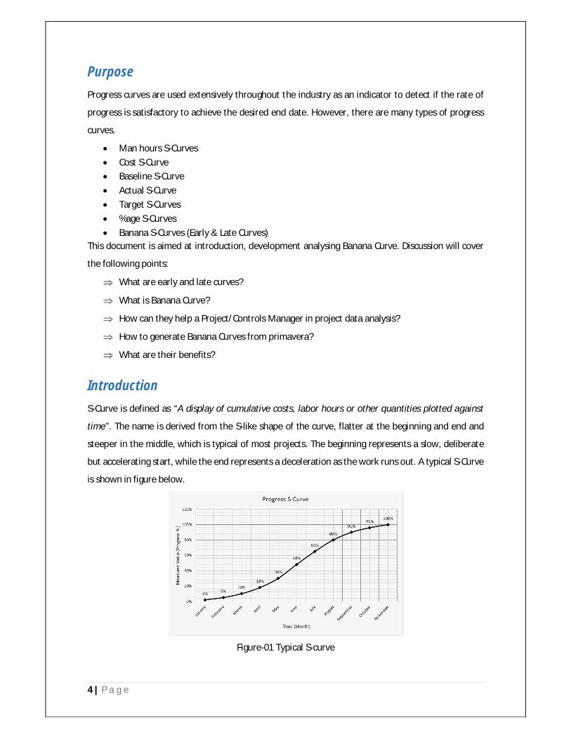
Introduction S-Curve is defined as “A display of cumulative costs, labor hours or other quantities plotted against

time”. The name is derived from the S-like shape of the curve, flatter at the beginning and end and

steeper in the middle, which is typical of most projects. The beginning represents a slow, deliberate

but accelerating start, while the end represents a deceleration as the work runs out. A typical S-Curve

is shown in figure below.

Figure-01 Typical S-curve

5 | P a g e

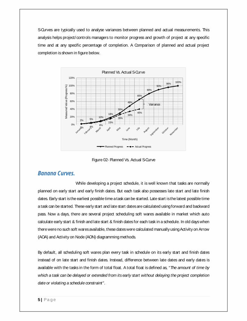
S-Curves are typically used to analyse variances between planned and actual measurements. This

analysis helps project/controls managers to monitor progress and growth of project at any specific

time and at any specific percentage of completion. A Comparison of planned and actual project

completion is shown in figure below.

Figure 02- Planned Vs. Actual S-Curve

Banana Curves. While developing a project schedule, it is well known that tasks are normally

planned on early start and early finish dates. But each task also possesses late start and late finish

dates. Early start is the earliest possible time a task can be started. Late start is the latest possible time

a task can be started. These early start and late start dates are calculated using forward and backward

pass. Now a days, there are several project scheduling soft wares available in market which auto

calculate early start & finish and late start & finish dates for each task in a schedule. In old days when

there were no such soft wares available, these dates were calculated manually using Activity on Arrow

(AOA) and Activity on Node (AON) diagramming methods.

By default, all scheduling soft wares plan every task in schedule on its early start and finish dates

instead of on late start and finish dates. Instead, difference between late dates and early dates is

available with the tasks in the form of total float. A total float is defined as, “The amount of time by

which a task can be delayed or extended from its early start without delaying the project completion

date or violating a schedule constraint”.

2% 5%10%

18%

30%

48%

65%

80%90%

96% 100%

2% 4% 8%15%

26%34%

40%

0%

20%

40%

60%

80%

100%

120%

Mea

sure

d Va

lue

(Pro

gres

s % )

Time (Month)

Planned Vs. Actual S-Curve

Planned Progress Actual Progress

Variance

6 | P a g e

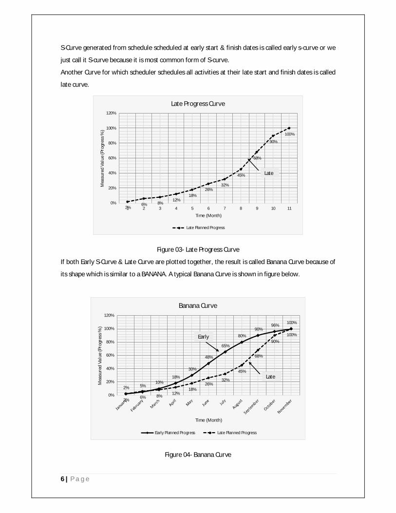
S-Curve generated from schedule scheduled at early start & finish dates is called early s-curve or we

just call it S-curve because it is most common form of S-curve.

Another Curve for which scheduler schedules all activities at their late start and finish dates is called

late curve.

Figure 03- Late Progress Curve

If both Early S-Curve & Late Curve are plotted together, the result is called Banana Curve because of

its shape which is similar to a BANANA. A typical Banana Curve is shown in figure below.

Figure 04- Banana Curve

2%6% 8%

12%18%

26%32%

45%

68%

90%

100%

0%

20%

40%

60%

80%

100%

120%

1 2 3 4 5 6 7 8 9 10 11

Mea

sure

d Va

lue

(Pro

gres

s % )

Time (Month)

Late Progress Curve

Late Planned Progress

Late

2% 5%10%

18%

30%

48%

65%

80%90%

96% 100%

2% 6% 8% 12%18%

26%32%

45%

68%

90%100%

0%

20%

40%

60%

80%

100%

120%

Mea

sure

d Va

lue

(Pro

gres

s % )

Time (Month)

Banana Curve

Early Planned Progress Late Planned Progress

Early

Late

7 | P a g e

When actual data is fed into schedule and schedule is updated, Actual progress line should float

between early and late curves or within banana curve. Actual Progress line above banana will show

that project is either ahead of schedule (if banana curve is for progress) or above budget (if banana

curve is for cost) and actual line below banana curve will show that project is either behind schedule

or under budget.

Figure 05- Banana Vs. Actual

This approach is a nice example of “management by exception”. The rule is that “the actual progress

line should be within the banana”. If the line is going outside of the banana, project/controls manager

has to manage it. It is an exception to the rule. Having a swift glimpse of this report, the manager can

have a good idea of the standing of the project as compared to where it was planned to be. This

approach can be used as an early warning to make a manager vigilant about any cash issues showing

up on the Project.

Sometimes upper level management keeps this report favourite. Every scheduling soft wares available

in market does not have capability to generate banana curve. Using Microsoft Project, you can

generate only one curve at a time i.e. early curve or late curve. MS Project does not have capability to

combine both curves. Primavera Project Planner (P6) has capability to generate “early curve” and “late

curve” at the same time which results in the formation of banana curve. You can also prepare banana

curve in excel by exporting data from primavera P6 to excel. In this document, different methods of

generating banana curve from primavera schedule will be discussed. Our reference throughout the

discussion will be “baseline schedule” not an “As build schedule”.

2% 5%10%

18%

30%

48%

65%

80%90%

96%100%

2% 6% 8% 12%18%

26%32%

45%

68%

90%100%

0%

20%

40%

60%

80%

100%

120%

Mea

sure

d Va

lue

(Pro

gres

s % )

Time (Month)

Banana Vs. Actual

Early Planned Progress Late Planned Progress Actual Progress

Early

Late

8 | P a g e

Methods to Calculate Early and Late curves data in primavera schedule.

In this document, we will discuss four methods to calculate early and late cash flow in primavera

schedule.

1. Using Activity Usage Profile

2. Using Reports tool.

3. Using Activity Usage Spread Sheet

4. Using Resource Assignment Data

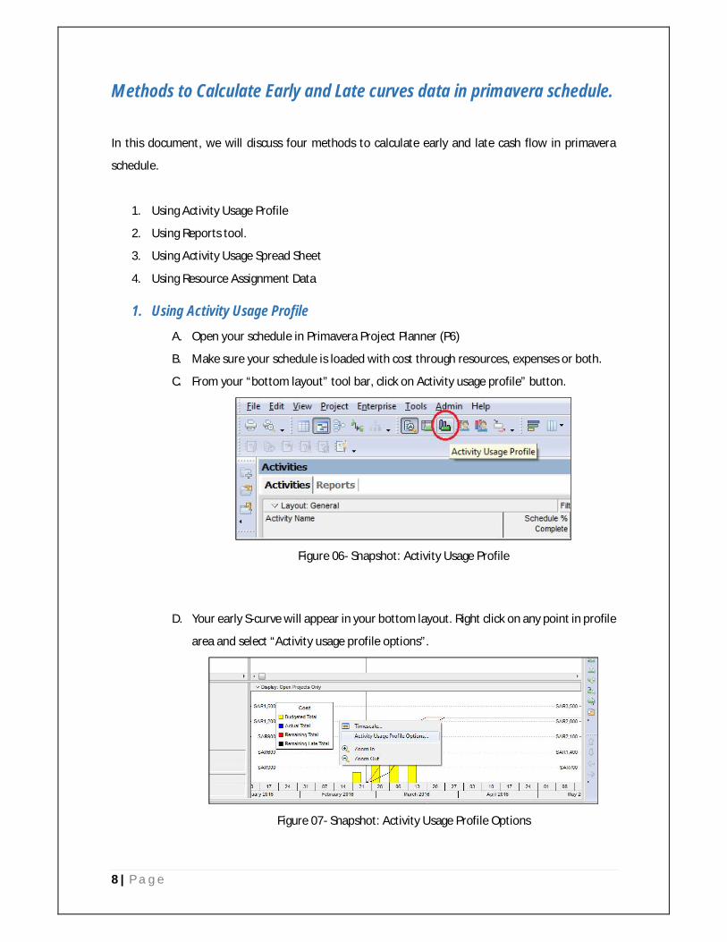
1. Using Activity Usage Profile

A. Open your schedule in Primavera Project Planner (P6)

B. Make sure your schedule is loaded with cost through resources, expenses or both.

C. From your “bottom layout” tool bar, click on Activity usage profile” button.

Figure 06- Snapshot: Activity Usage Profile

D. Your early S-curve will appear in your bottom layout. Right click on any point in profile

area and select “Activity usage profile options”.

Figure 07- Snapshot: Activity Usage Profile Options

9 | P a g e

E. From Activity usage profile option window, select “Cost” if you need banana curve for

your cash flow and select “Unit” if you need banana curve for you resource units.

Then select types of cost or units you want to bring into banana curve. After that in

“Show Bar/Curve” section, check boxes of “Remaining Early” & “Remaining Late”

option under cumulative boxes. Press Apply and then OK.

Figure 08- Snapshot: Selecting Data from Activity Usage Profile Options.

F. Now you will get banana curve in your profile area as shown in the following figure.

Figure 09 – Snapshot: Early and Late Curves in Primavera P6.

10 | P a g e

2. Using Reports tool.

Although Banana Curves can be drawn in P6 itself, but primavera has very limited profile and data

enhancement options. Data labelling is also not adjustable and graphics are not that much attractive.

To create more attractive graphs, some of the professionals use MS Excel to draw graphs by exporting

data from p6 through reports tool and some other methods which also be discussed later. By default,

report tool provides data only for early dates. So here we have to extract data in two steps. To

complete this action, follow given steps.

Step1: Exporting Early Curve Data

A. Click on “Tools” on main manue and go to reports as shown in the figure.

Figure 10 – Snapshot: Selecting Report Tool.

B. From reports window click on any report and press “+” button to add or modify

report.

C. Report Wizard will open. Click next and check “Time Distributed Data” checkbox. Now

from given field select “activities” and click next.

Figure 11 – Snapshot: Subject Area Selection

11 | P a g e

D. Now “Configure Selected Subject Areas” window will open. Click on “Columns” button

and select “Planned Value Cost” and click OK.

Figure 12- Snapshot: Configuring Selected Subject Area

E. On next screen adjust timescale and click “Next”.

F. Write appropriate report title and click “Next”.

G. Click on “Run Report”.

H. In “Run Report” window, select HTML file, select file output location and click “OK” as

shown in figure.

Figure 13 – Snapshot: Selection of Report Format and Output Location.

12 | P a g e

I. Report will open in your web browser. Here you can select values, paste in excel and

draw nice and attractive graph.

Step 2: Exporting Late Curve Data

A. Now you have data for early curve only. To get data for late curve, you have to schedule all

activities on their latest dates.

B. To get late curve data, go to columns and insert “Primary Constraint”.

C. In this column, select “As late as Possible” constraint for the first activity.

D. Use fill down option to assign this constraint to all activities.

E. Press F9 to schedule.

F. Now all activities are scheduled at their late dates.

G. Repeat the same steps as you did to get data for early dates.

H. Combine both early and late curves in MS excel to generate nice and attractive banana curve.

---------------------------------------------------------------------------------------------------------------

13 | P a g e

3. Using Activity Usage Spreadsheet

MS Excel has wealth of options to adjust and manage graphs and make them easy to understand and

attractive. Follow given steps to create banana curve by exporting data from “activity usage

spreadsheet”.

A. To export data to excel, click on “activity usage spread sheet” button and you will have it in

your bottom layout.

Figure 14 – Snapshot: Activity Usage Spreadsheet in Primavera P6.

B. In spread sheet opened in your bottom lay out, move cursor to the upper left corner of

spreadsheet and right click. From options select “Spreadsheet fields”.

Figure 15 – Snapshot: Selecting Spreadsheet Fields.

C. From “Spreadsheet options” window select “Cum Budgeted Total Cost” and “Cum remaining

late total cost”. “Cum Budgeted Total Cost” will give you values which are already calculated

at early dates while “Cum remaining late total cost” will give you values calculated on late

dates of schedule.

See figure below.

14 | P a g e

Figure 16 – Snapshot: Selecting Early and Late Cost Data from P6.

D. Now you have both “Cum Budgeted Total Cost” and “Cum remaining late total cost” values

in your bottom layout. Click on the upper left corner and press Ctrl+C on your keyboard to

copy data. Don’t forget to adjust time intervals from timescale according to your

requirements.

Figure 17 – Snapshot: Copying Data from Activity Usage Spreadsheet

E. Now you can paste this data in excel and create nice looking and attractive banana curve.

------------------------------------------------------------------------------------------------------------------------------

15 | P a g e

4. Using Resource Assignment Data

If you have loaded all of your cost in resources and there is no expense cost in your schedule, you can

use this method to extract early and late data and transfer to MS excel to create banana curve. This is

most easy and handy method. To extract data through resource assignments, complete following

steps.

A. Click on “Resource assignments” button.

Figure 18 – Snapshot: Resource Assignments

B. Right click in resource assignment spreadsheet area and select “Cum Remaining Early Cost”

and “Cum Remaining Late Cost” options. Click “OK” to apply changes.

Figure 19 – Snapshot: Selecting Early and Late data from resource assignments.

C. In Resource Assignment Window, select the resource pool for which you want to have early

and late costs and press Ctrl+C to copy data.

D. Go to excel and past this data. Now you can play with this data to draw banana curve in excel

as shown in figure.

Figure 20 – Snapshot: Sample Banana Curve in MS Excel

16 | P a g e

References

Online References

www.maxwideman.com

www.planacademy.com

www.planningplannet.com

Book Reference

Construction Project Scheduling & Control 3rd Edition. (Saleh Mubarak)

Construction Scheduling – Principles and Practices (J.S Newitt)

Project Planning & Control using Primavera P6 (Paul Eastwood Harris)