Introduction à R

Olivier Mestre

Ecole Nationale de la Météorologie

R on the web

• Main ressource

http://www.r-project.org/

• Mirrors

example : Toulouse (CICT, UPS)

http://cran.cict.fr/

Characteristics

• Advantages– Free– Available on UNIX, LINUX, WINDOWS– Dedicated to statistics, graphical capabilities– open source

• Inconvénients– Bugs (always possible)– Beware memory size in climate applications

Running R

• Install R : download from website

• Running R : simply type R

• Quit R (sniff) : type q( ).

Sessions and programs

• Interactive sessions

• Programs : command files

source(“prog.R”)

• Shell UNIX (mode batch) :

R CMD BATCH prog.R

Help

• Full documentation on CRAN

• Use “search” on CRAN

• R session : ?command

example: ?sd

sd : entering a command gives its source code.

Installing “packages” (linux)

• Package = true reason of R usefulness

• Export R_LIBS variable in your “.profile” (library directory).

• Example : install sudoku package (to be done once)install.packages(“sudoku”,dependencies=TRUE)

• Load sudoku in your session (necessary each time you want to use it).library(sudoku)

Basic commands

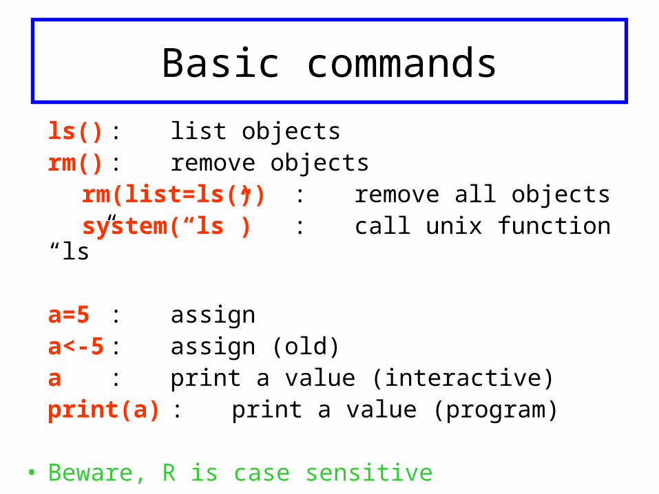
ls() : list objectsrm() : remove objects

rm(list=ls()) : remove all objects system(“ls”) : call unix function “ls”

a=5 : assigna<-5 : assign (old)a : print a value (interactive)print(a) : print a value (program)

• Beware, R is case sensitive

Special characters

# Comments

; Separates two commands on the same line.

“ “ Strings

pi 3,141593..

Arithmétics

+ : addition

- : substraction, sign

* : multiplication

/ : division

^ : power

%/% : integer division

%% : remainder from integer division

Logical

== : equal to!= : no equal to < : less than> : greater than<= : less than or equal to>= : greater than or equal tois.na() : missing?& : logical AND| : logical OR! : logical NOT

Conversion

as.numeric(x) conversion to numericas.integer(x) conversion to integeras.character(x) conversion to stringas.logical(x) conversion to logicalas.matrix(x)

is.numeric(x),is.integer(x)… gives TRUE if numeric or integer variable, FALSE. Beware : integer is also numeric, while numeric may be different from integer.

Strings

• Paste function

num.fic = 1

n.fic = as.character(numero.fichier)

nom.fichier=paste(“fichier”,n.fic,”.txt”,sep=“”)• nchar,substr functions

a=“abcdefg”

nchar(a)

substr(a,1,3)

substr(a,1,4)=“123456”

Generating

numeric(25) : 25 zéros (vector)character(25) : 25 “” vector of empty

stringsseq(-4,4,0.1) : sequence -4.0 -3.9 … 4.01:10 : idem seq(1,10,1)1:10-3 : Arf!1:(10-3) : Arf!c(5,7,1:3) : concatenation 5 7 1 2 3rep(1,7) : replication 1 1 1 1 1 1

Matrix generating

matrix(0,nrow=3,ncol=4)

matrix(1:12,nrow=3,ncol=4)

matrix(1:12,nrow=3,ncol=4, byrow=TRUE)

Data frames

Allow mixing different data types in the same object. All variables must have same length

donnee=data.frame(an=1880:2005,TN,TX)

donnee=data frame made of 3 vectors of same length :

donnee$an, donnee$TN, donnees$TX

Data frames

names(donnee) : names of the variables in “donnee”

attach(donnee) : allows direct call of variables : “an” instead of “donnee$an”. Beware there is no link between those variables in case of modifications

detach(donnee) : opposite to attach()

Lists

• List = “composite” object

• Useful for function results

toto=list(y=an,titi,tata)

names(toto) : nom des objets dans toto

Exercise

• Create a data frame containing two variables :

“an” : years 1880, 1881,…, 2000

“bis” : logical, indicating wether year has 365 (FALSE) or 366 days (TRUE)

Hint : use reminder of division by 4

Classical functions

• x may be scalar of vector (in the latter case, the result is a vector).round(x,k) : rounding x (k digits)

log(x) : natural loglog10(x) : log base 10sqrt(x) : square rootexp(x)sin(x),cos(x),tan(x)asin(x),acos(x),atan(x)

Functions on vectors

length(x) : size of x

min(x), min(x1,x2) : gives the minimum of x (or x1,x2) max(x) : same as min, for maximum

pmin(x1,x2..,xk) : gives k minima of x1, x2… xkpmax(x1,x2,…, xk) : same as pmin for maxima

sort(x) : sorting x (if index.return=TRUE, gives also the corresponding indices)

Some statistics

sum(x) : sum of x elements

mean(x) : mean of x elements

var(x) : variance

sd(x) : standard deviation

median(x) : médian

quantile(x,p) : p quantile

cor(x,y) :correlation between x and y

Indexing, selection

x[1] : first element of x

x[1:5] : 5 first elements

x[c(3,5,6)] : elements 3,5,6 of x

z=c(3,5,6) ; x[z] : idem

x[x>=5] : elements of x 5

L=x>=5 ; x[L] : idem

i=which(x>=5);x[i] : idem

Matrices

m[i,] : ith line

m[,j] : jth column

• Selection columns or lines == vectors

m1%*%m2 : matrix multiplication

solve(m) : matrix inversion

svd(m) : SVD

Matrices

rbind, cbind allow adding rows (rbind) or columns (cbind) to a vector, matrix or data frame

y=rep(1,10);z=seq(1,1)

M=cbind(y,z)

remove M second column

M[,-2]

remove rows 4 and 6

M[c(-4,-6), ]

Indexing Frames

donnee[donnee$annee<=1940,]

subset of “donnee” corresponding to years before 1941

subset(donnee,annee<=1940)

idem

Programming

if (toto==2){tata=1}

if (toto==2){tata=1}

else{tata=0}

Programmingfor (i in 1:10)

{ tata[i]=exp(toto[i])}

Beware, “:” has priority, compare 1:10-1 and 1:(10-1)

i=1while (i < 10)

{tata[i]=exp(toto[i]) i=i+1}

Functions

• Definition

ect=function(x)

{resultat=sqrt(var(x)

return(resultat)}

• Call

s=ect(x)

Functions

• Lists in fuctions

moyect=function(x)

{s=ect(x)

m=mean(x)

resultat=list(moyenne=m,ect=s)

return(resultat)}

Read data

• Interactive

a=readline(“donner la valeur de a ”)

• Read ASCII file with header

data=read.table(file=“nomfic”,header=TRUE)

• Write ASCII file (use format and round)

write.table(format(round(data,k)),quote=F

file=“nomfic”,sep=“ ”,rownames=F)

Saving objects

save(a,m,file=“toto.sav”)

load(“toto.sav”)

Distributions

• Normal law, expectation m, sd s

dnorm(x,m,s) : density de x

pnorm(x,m,s) : repartition function

qnorm(p,m,s): p quantile

rnorm(n,m,s) : random number generation

Distributions

• Convention : d=density, p=repartition, q=quantile,r=random

• unif(,min,max) uniform on [min,max]

• pt(,df) Student(df)

• chisq(,df) ²(df)

• f(,d1,d2) Fisher(d1,d2)

• pois(,lambda) Poisson(lambda)

• Etc..

Figures

• Open device :

x11() : window on screen

postscript(file=“fig.eps”) : postscript

png(file=“fig.png”) : PNG

• Plot ()

• Close device

graphics.off() : close windows or finalizes files

Figures

• Plot()

plot(x,y,type=“l”,main=“toto”,…)• Parameters

type=“l” (line),”p” (point),”h” (vertical line)…

main=“title”,xlab=“title x”,ylab=“title y”,sub=“subtitle”– xlim=[a,b],ylim=[c,d]. Beware, R adds 4% to axis. Add

xaxs=“i”,yaxs=“i”, for exact setting of axis range– col=“red” colors() for list

Controlling lines and symbols

lwd=line width

lty=line type (dots, etc…)

pch=“+”, “.”,”*” etc..

?par lists parameters an use

Other plotting functions

lines(x,y) : adds linespoints(x,y) : pointstext(x,y,”texte”) : adds text at x,yabline(a,b) : straight line y=ax+babline(h=y) : horizontale line (height=y)abline(v=x) : vertical line (position=x)

See also : legendEtc…

Infinite capabilities

• Multiple figures

• 2D contours

• 3D (lattice)

• Maps (package “map”)

Exercise

• Draw density of N(0,1)– generate x from -5 to +5 (step : 0.01)– Calculate and plot density of normal law N(0,1)

Exercise

• Central-limit theorem– Generate 1000 vectors of size 12 following

uniform law U[0,1] – command hist() : histogram of generated

values– Calculate means of the 1000 vectors, and

represent their histogram– Same questions for an exponential law of rate

10

Magic!

Exercise

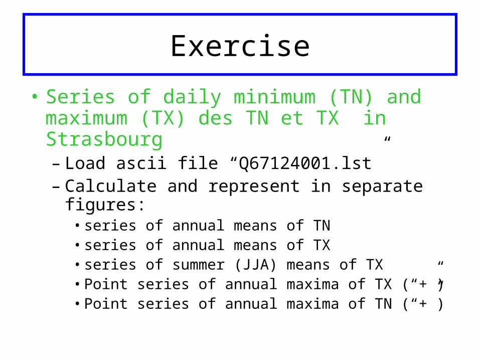
• Series of daily minimum (TN) and maximum (TX) des TN et TX in Strasbourg– Load ascii file “Q67124001.lst” – Calculate and represent in separate figures:

• series of annual means of TN• series of annual means of TX• series of summer (JJA) means of TX• Point series of annual maxima of TX (“+”)• Point series of annual maxima of TN (“+”)

Exercise

• Series of annual number of frost days– Calculate and plot this series

– command summary() : basic statistics on this series

– command hist() : histogrma of the annual number of frost days

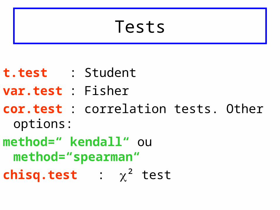
Tests

t.test : Student

var.test : Fisher

cor.test : correlation tests. Other options:

method=“ kendall“ ou method=“spearman“

chisq.test : ² test

Gaussian linear model

lm(y~x) : y explained by x

lm(y~x1+x2): y explained by x1, x2

f=as.factor(f) : transforms f into a factor

lm(y~f) : one factor ANOVA

lm(y~f1+f2) : two factors ANOVA

lm(y~x+f) : covariance analysis

Formula, interactions

~ : explained by

+ : additive effects

: : interaction

* : effects + interactions

a * b = a + b + a:b

-1 : removes intercept

Outputs

lm.out=lm(y~x) : results in lm.out object

summary(lm.out) : coefficients, tests, etc..

anova(lm.out) : regression sum of squares

plot(lm.out) : plot diagnosis

fitted(lm.out) : fitted values

residuals(lm.out) : residuals

predict(lm.out,newdata) : prediction for a new data frame

GLM

• Families : ?family

• Logistic regressionglm.out=glm(y~x, binomial)

• Poisson régressionglm.out=glm(y~x, poisson)

• Remark:lm(y~x) equivalent to glm(y~x, gaussian)

Outputs

summary(lm.out) : coefficients, tests, etc..

fitted(lm.out) : fitted values

residual(lm.out) : residuals

predict(lm.out,newdata) prediction for a new data frame