introduc)on to bayesian methods (connued) - lecture...
TRANSCRIPT
Introduc)ontoBayesianmethods(con)nued)-Lecture16
DavidSontagNewYorkUniversity
Slides adapted from Luke Zettlemoyer, Carlos Guestrin, Dan Klein, and Vibhav Gogate
Outlineoflectures
• Reviewofprobability
(A?ermidterm)
Maximumlikelihoodes)ma)on
2examplesofBayesianclassifiers:
• NaïveBayes• LogisIcregression
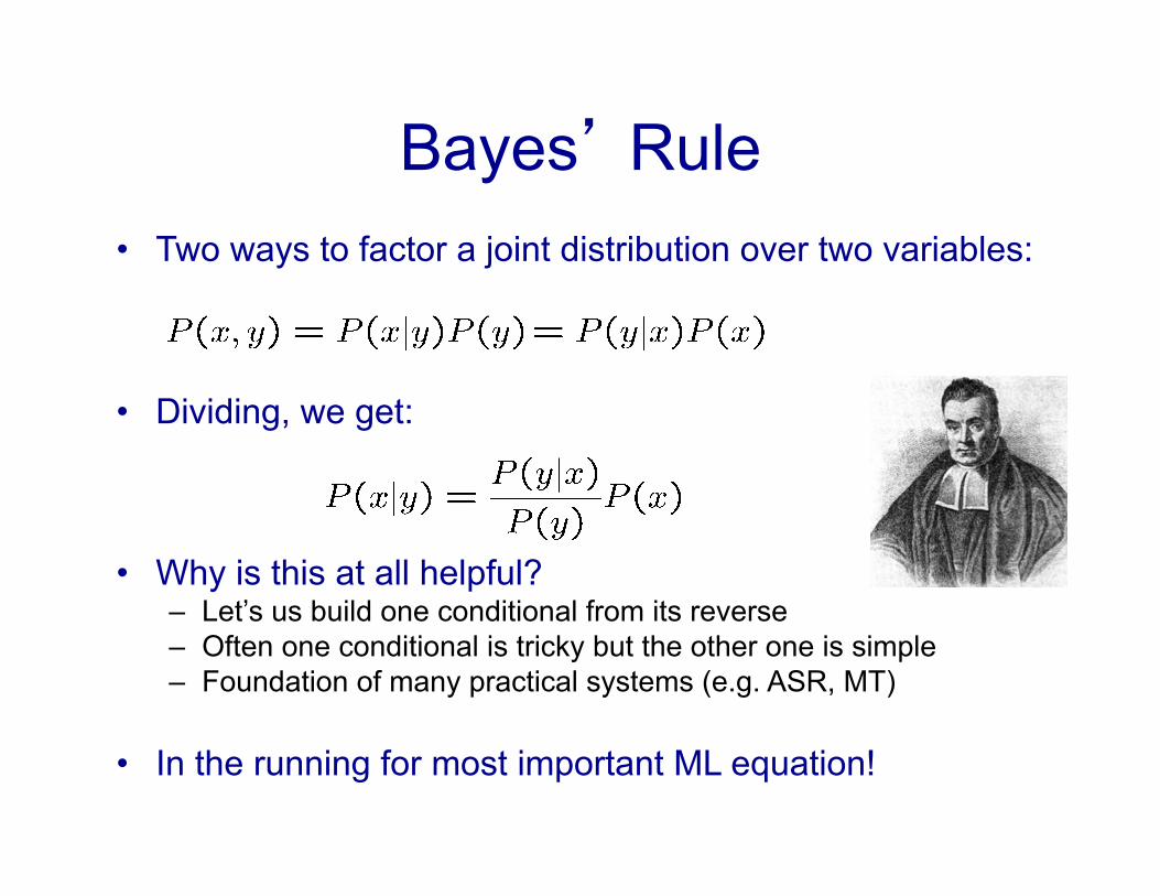
Bayes’ Rule • Two ways to factor a joint distribution over two variables:
• Dividing, we get:
• Why is this at all helpful? – Let’s us build one conditional from its reverse – Often one conditional is tricky but the other one is simple – Foundation of many practical systems (e.g. ASR, MT)
• In the running for most important ML equation!
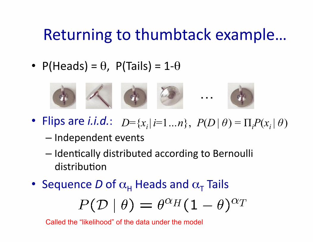
Returningtothumbtackexample…
• P(Heads)=θ,P(Tails)=1-θ
• Flipsarei.i.d.:– Independentevents– IdenIcallydistributedaccordingtoBernoullidistribuIon
• SequenceDofαHHeadsandαTTails
…
D={xi | i=1…n}, P(D | θ ) = ΠiP(xi | θ )
Called the “likelihood” of the data under the model
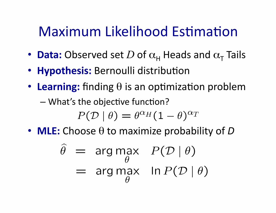
MaximumLikelihoodEsImaIon• Data:ObservedsetDofαHHeadsandαTTails• Hypothesis:BernoullidistribuIon• Learning:findingθ isanopImizaIonproblem
– What’stheobjecIvefuncIon?
• MLE:ChooseθtomaximizeprobabilityofD
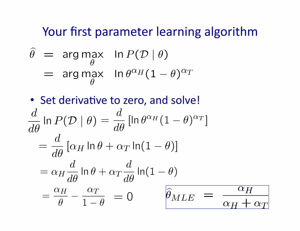
Yourfirstparameterlearningalgorithm
• SetderivaIvetozero,andsolve!
Brief Article
The Author
January 11, 2012
ˆ⇥ = argmax
⇥lnP (D | ⇥)
ln ⇥�H
d
d⇥lnP (D | ⇥) =
d
d⇥[
ln ⇥�H(1� ⇥)�T
]
=
d
d⇥[
�H ln ⇥ + �T ln(1� ⇥)]
1
Brief Article
The Author
January 11, 2012
ˆ⇥ = argmax
⇥lnP (D | ⇥)
ln ⇥�H
d
d⇥lnP (D | ⇥) =
d
d⇥[
ln ⇥�H(1� ⇥)�T
]
=
d
d⇥[
�H ln ⇥ + �T ln(1� ⇥)]
1
Brief Article
The Author
January 11, 2012
ˆ⇥ = argmax
⇥lnP (D | ⇥)
ln ⇥�H
d
d⇥lnP (D | ⇥) =
d
d⇥[
ln ⇥�H(1� ⇥)�T
]
=
d
d⇥[
�H ln ⇥ + �T ln(1� ⇥)]
= �Hd
d⇥ln ⇥ + �T
d
d⇥ln(1� ⇥) =
�H
⇥� �T
1� ⇥= 0
1
Brief Article
The Author
January 11, 2012
ˆ⇥ = argmax
⇥lnP (D | ⇥)
ln ⇥�H
d
d⇥lnP (D | ⇥) =
d
d⇥[
ln ⇥�H(1� ⇥)�T
]
=
d
d⇥[
�H ln ⇥ + �T ln(1� ⇥)]
= �Hd
d⇥ln ⇥ + �T
d
d⇥ln(1� ⇥) =
�H
⇥� �T
1� ⇥= 0
1
Brief Article
The Author
January 11, 2012
ˆ� = argmax
✓lnP (D | �)
ln �↵H
d
d�lnP (D | �) =
d
d�ln �↵H
(1� �)↵T
1
Brief Article
The Author
January 11, 2012
ˆ⇥ = argmax
⇥lnP (D | ⇥)
ln ⇥�H
d
d⇥lnP (D | ⇥) =
d
d⇥[
ln ⇥�H(1� ⇥)�T
]
=
d
d⇥[
�H ln ⇥ + �T ln(1� ⇥)]
= �Hd
d⇥ln ⇥ + �T
d
d⇥ln(1� ⇥) =
�H
⇥� �T
1� ⇥= 0
1
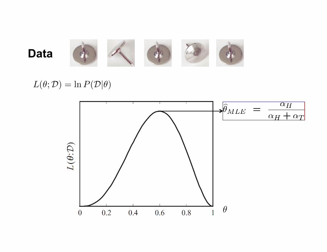
Data
✓
L(✓;D) = lnP (D|✓)
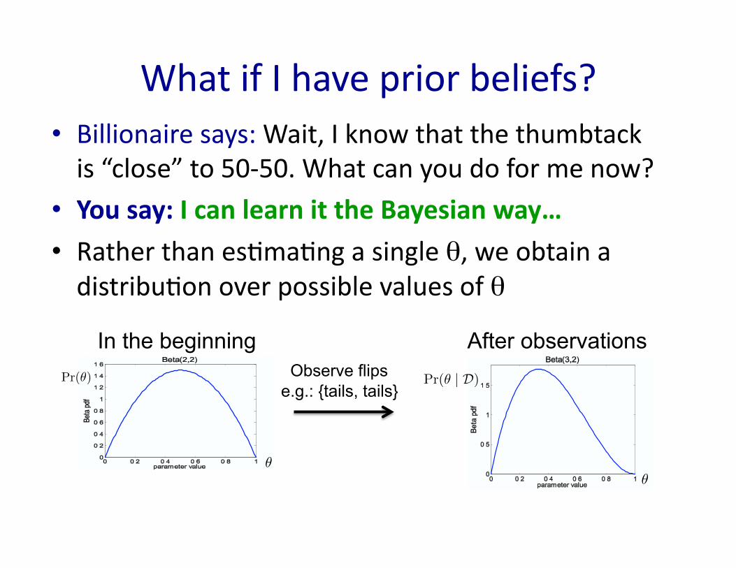
WhatifIhavepriorbeliefs?• Billionairesays:Wait,Iknowthatthethumbtackis“close”to50-50.Whatcanyoudoformenow?
• Yousay:IcanlearnittheBayesianway…• RatherthanesImaIngasingleθ,weobtainadistribuIonoverpossiblevaluesofθ
Observe flips e.g.: {tails, tails}
In the beginning
✓
Pr(✓)
After observations Pr(✓ | D)
✓
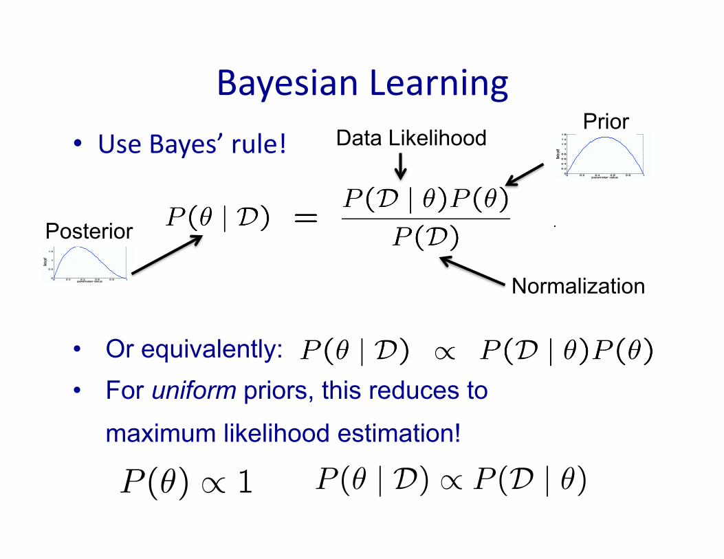
BayesianLearning
• UseBayes’rule!
• Or equivalently: • For uniform priors, this reduces to
maximum likelihood estimation!
Prior
Normalization
Data Likelihood
Posterior
Brief Article
The Author
January 11, 2012
ˆ⌅ = argmax
⇤lnP (D | ⌅)
ln ⌅�H
d
d⌅lnP (D | ⌅) =
d
d⌅[
ln ⌅�H(1� ⌅)�T
]
=
d
d⌅[
�H ln ⌅ + �T ln(1� ⌅)]
= �Hd
d⌅ln ⌅ + �T
d
d⌅ln(1� ⌅) =
�H
⌅� �T
1� ⌅= 0
⇥ ⇤ 2e�2N⇥2 ⇤ P (mistake)
ln ⇥ ⇤ ln 2� 2N⇤2
N ⇤ ln(2/⇥)
2⇤2
N ⇤ ln(2/0.05)2⇥ 0.12 ⌅ 3.8
0.02= 190
P (⌅) ⇧ 1
1
Brief Article
The Author
January 11, 2012
ˆ⌅ = argmax
⇤lnP (D | ⌅)
ln ⌅�H
d
d⌅lnP (D | ⌅) =
d
d⌅[
ln ⌅�H(1� ⌅)�T
]
=
d
d⌅[
�H ln ⌅ + �T ln(1� ⌅)]
= �Hd
d⌅ln ⌅ + �T
d
d⌅ln(1� ⌅) =
�H
⌅� �T
1� ⌅= 0
⇥ ⇤ 2e�2N⇥2 ⇤ P (mistake)
ln ⇥ ⇤ ln 2� 2N⇤2
N ⇤ ln(2/⇥)
2⇤2
N ⇤ ln(2/0.05)2⇥ 0.12 ⌅ 3.8
0.02= 190
P (⌅) ⇧ 1
P (⌅ | D) ⇧ P (D | ⌅)
1
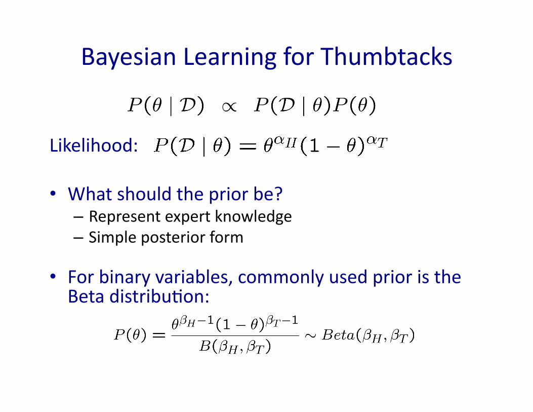
BayesianLearningforThumbtacks
Likelihood:
• Whatshouldthepriorbe?– Representexpertknowledge– Simpleposteriorform
• Forbinaryvariables,commonlyusedprioristheBetadistribuIon:

= ✓↵H+�H�1 (1� ✓)↵T+�T�1
BetapriordistribuIon–P(θ)
• SincetheBetadistribuIonisconjugatetotheBernoullidistribuIon,theposteriordistribuIonhasaparIcularlysimpleform:
Brief Article
The Author
January 11, 2012
ˆ⌅ = argmax
⌅lnP (D | ⌅)
ln ⌅�H
d
d⌅lnP (D | ⌅) =
d
d⌅[
ln ⌅�H(1� ⌅)�T
]
=
d
d⌅[
�H ln ⌅ + �T ln(1� ⌅)]
= �Hd
d⌅ln ⌅ + �T
d
d⌅ln(1� ⌅) =
�H
⌅� �T
1� ⌅= 0
⇥ ⇤ 2e�2N⇤2 ⇤ P (mistake)
ln ⇥ ⇤ ln 2� 2N⇤2
N ⇤ ln(2/⇥)
2⇤2
N ⇤ ln(2/0.05)2⇥ 0.12 ⌅ 3.8
0.02= 190
P (⌅) ⇧ 1
P (⌅ | D) ⇧ P (D | ⌅)
P (⌅ | D) ⇧ ⌅�H(1� ⌅)�T ⌅⇥H�1
(1� ⌅)⇥T�1
1
Brief Article
The Author
January 11, 2012
ˆ⇧ = argmax
⌅lnP (D | ⇧)
ln ⇧�H
d
d⇧lnP (D | ⇧) =
d
d⇧[
ln ⇧�H(1� ⇧)�T
]
=
d
d⇧[
�H ln ⇧ + �T ln(1� ⇧)]
= �Hd
d⇧ln ⇧ + �T
d
d⇧ln(1� ⇧) =
�H
⇧� �T
1� ⇧= 0
⇤ ⇤ 2e�2N⇤2 ⇤ P (mistake)
ln ⇤ ⇤ ln 2� 2N⌅2
N ⇤ ln(2/⇤)
2⌅2
N ⇤ ln(2/0.05)2⇥ 0.12 ⌅ 3.8
0.02= 190
P (⇧) ⇧ 1
P (⇧ | D) ⇧ P (D | ⇧)
P (⇧ | D) ⇧ ⇧�H(1�⇧)�T ⇧⇥H�1
(1�⇧)⇥T�1= ⇧�H+⇥H�1
(1�⇧)�T+⇥t+1= Beta(�H+⇥H , �T+⇥T )
1
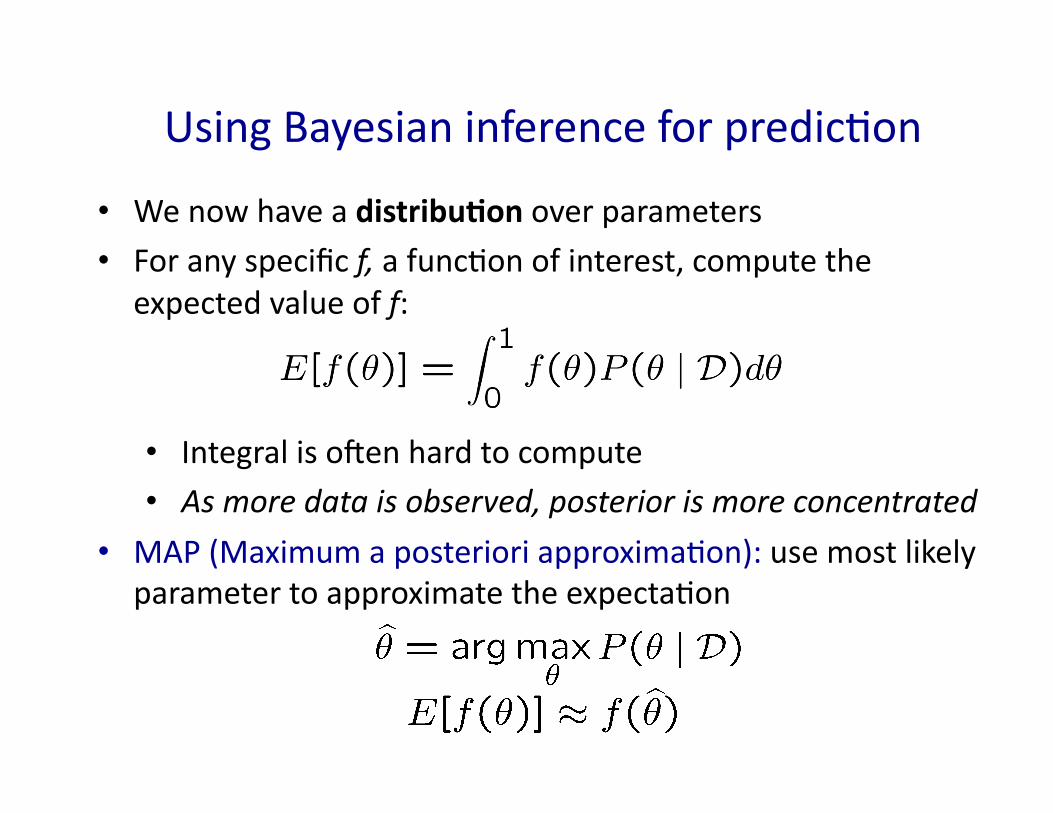
• Wenowhaveadistribu)onoverparameters• Foranyspecificf,afuncIonofinterest,computethe
expectedvalueoff:
• Integraliso?enhardtocompute• Asmoredataisobserved,posteriorismoreconcentrated
• MAP(MaximumaposterioriapproximaIon):usemostlikelyparametertoapproximatetheexpectaIon
UsingBayesianinferenceforpredicIon

Outlineoflectures
• Reviewofprobability• MaximumlikelihoodesImaIon
2examplesofBayesianclassifiers:
• NaïveBayes• LogisIcregression

BayesianClassificaIon
• Problemstatement:– GivenfeaturesX1,X2,…,Xn– PredictalabelY
[Next several slides adapted from: Vibhav Gogate, Jonathan Huang, Luke Zettlemoyer, Carlos
Guestrin, and Dan Weld]

ExampleApplicaIon
• DigitRecogni)on
• X1,…,Xn∈{0,1}(Blackvs.Whitepixels)
• Y∈{0,1,2,3,4,5,6,7,8,9}
Classifier 5
X Y
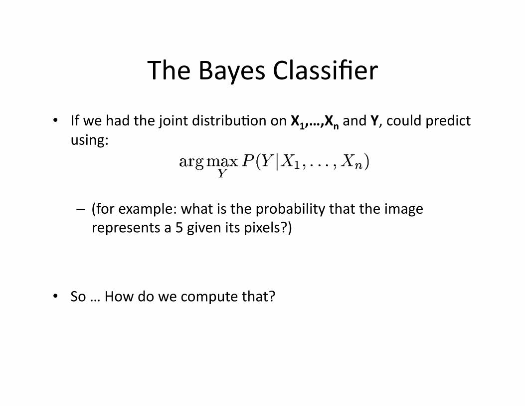
TheBayesClassifier
• IfwehadthejointdistribuIononX1,…,XnandY,couldpredictusing:
– (forexample:whatistheprobabilitythattheimagerepresentsa5givenitspixels?)
• So…Howdowecomputethat?
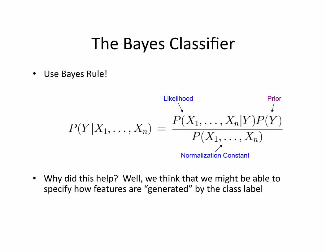
TheBayesClassifier
• UseBayesRule!
• Whydidthishelp?Well,wethinkthatwemightbeabletospecifyhowfeaturesare“generated”bytheclasslabel
Normalization Constant
Likelihood Prior
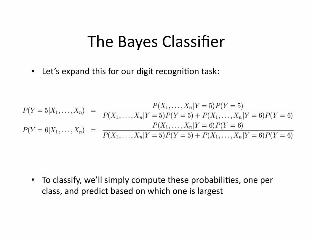
TheBayesClassifier
• Let’sexpandthisforourdigitrecogniIontask:
• Toclassify,we’llsimplycomputetheseprobabiliIes,oneperclass,andpredictbasedonwhichoneislargest
ModelParameters
• Howmanyparametersarerequiredtospecifythelikelihood,P(X1,…,Xn|Y)?
– (Supposingthateachimageis30x30pixels)
• TheproblemwithexplicitlymodelingP(X1,…,Xn|Y)isthatthereareusuallywaytoomanyparameters:
– We’llrunoutofspace
– We’llrunoutofIme– Andwe’llneedtonsoftrainingdata(whichisusuallynotavailable)
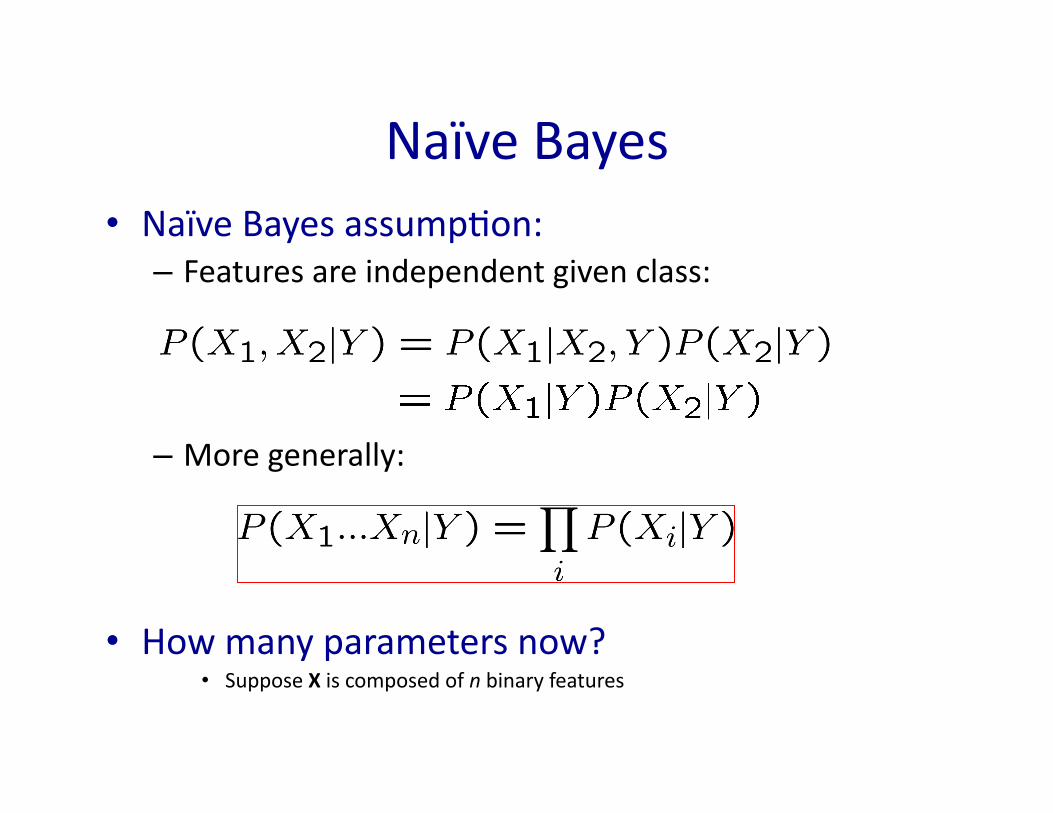
NaïveBayes• NaïveBayesassumpIon:
– Featuresareindependentgivenclass:
– Moregenerally:
• Howmanyparametersnow?• SupposeXiscomposedofnbinaryfeatures
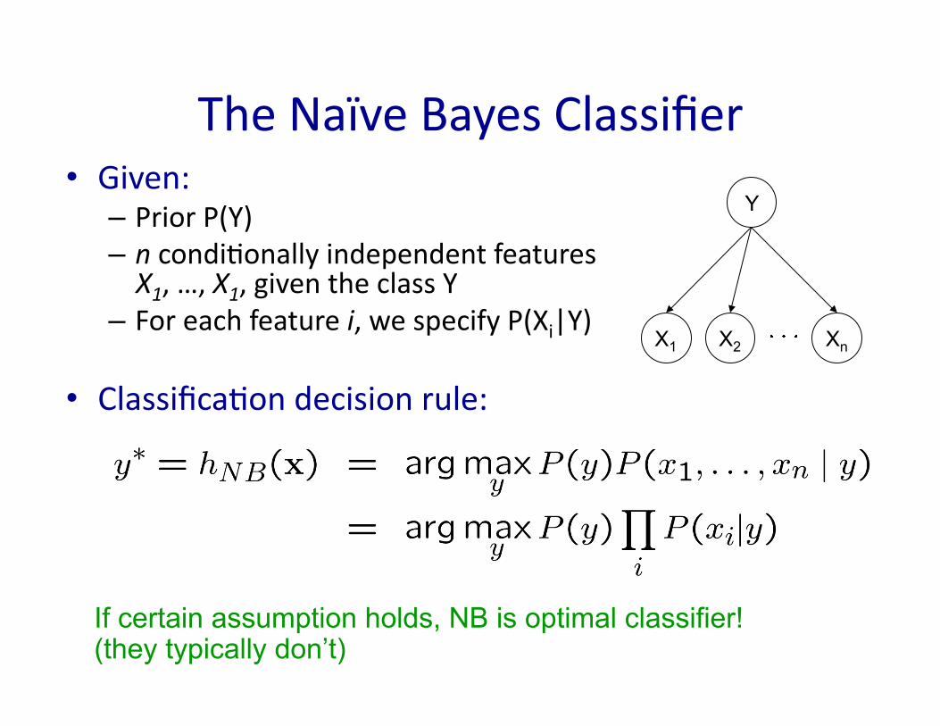
TheNaïveBayesClassifier• Given:
– PriorP(Y)– ncondiIonallyindependentfeaturesX1,…,X1,giventheclassY
– Foreachfeaturei,wespecifyP(Xi|Y)
• ClassificaIondecisionrule:
If certain assumption holds, NB is optimal classifier! (they typically don’t)
Y
X1 Xn X2
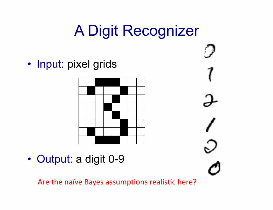
A Digit Recognizer
• Input: pixel grids
• Output: a digit 0-9
ArethenaïveBayesassumpIonsrealisIchere?
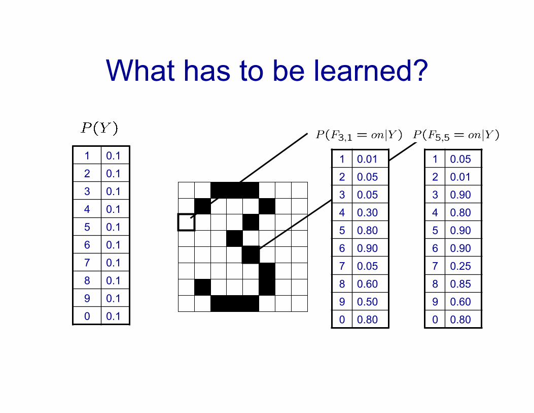
What has to be learned?
1 0.1 2 0.1 3 0.1 4 0.1 5 0.1 6 0.1 7 0.1 8 0.1 9 0.1 0 0.1
1 0.01 2 0.05 3 0.05 4 0.30 5 0.80 6 0.90 7 0.05 8 0.60 9 0.50 0 0.80
1 0.05 2 0.01 3 0.90 4 0.80 5 0.90 6 0.90 7 0.25 8 0.85 9 0.60 0 0.80
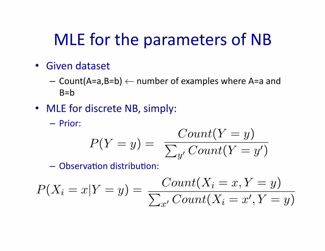
MLEfortheparametersofNB• Givendataset
– Count(A=a,B=b)ÃnumberofexampleswhereA=aandB=b
• MLEfordiscreteNB,simply:– Prior:
– ObservaIondistribuIon:
µMLE ,⇥MLE = argmaxµ,�
P (D | µ,⇥)
= �NX
i=1
(xi � µ)
⇥2= 0
= �NX
i=1
xi +Nµ = 0
= �N
⇥+
NX
i=1
(xi � µ)2
⇥3= 0
argmaxwln
✓1
⇥⇥2�
◆N
+NX
j=1
�[tj �P
iwihi(xj)]2
2⇥2
= argmaxw
NX
j=1
�[tj �P
iwihi(xj)]2
2⇥2
= argminw
NX
j=1
[tj �X
i
wihi(xj)]2
P (Y = y) =Count(Y = y)Py0 Count(Y = y�)
2
µMLE ,⇥MLE = argmaxµ,�
P (D | µ,⇥)
= �NX
i=1
(xi � µ)
⇥2= 0
= �NX
i=1
xi +Nµ = 0
= �N
⇥+
NX
i=1
(xi � µ)2
⇥3= 0
argmaxwln
✓1
⇥⇥2�
◆N
+NX
j=1
�[tj �P
iwihi(xj)]2
2⇥2
= argmaxw
NX
j=1
�[tj �P
iwihi(xj)]2
2⇥2
= argminw
NX
j=1
[tj �X
i
wihi(xj)]2
P (Y = y) =Count(Y = y)Py0 Count(Y = y�)
2
µMLE ,⇥MLE = argmaxµ,�
P (D | µ,⇥)
= �NX
i=1
(xi � µ)
⇥2= 0
= �NX
i=1
xi +Nµ = 0
= �N
⇥+
NX
i=1
(xi � µ)2
⇥3= 0
argmaxwln
✓1
⇥⇥2�
◆N
+NX
j=1
�[tj �P
iwihi(xj)]2
2⇥2
= argmaxw
NX
j=1
�[tj �P
iwihi(xj)]2
2⇥2
= argminw
NX
j=1
[tj �X
i
wihi(xj)]2
P (Y = y) =Count(Y = y)Py0 Count(Y = y�)
P (Xi = x|Y = y) =Count(Xi = x, Y = y)Px0 Count(Xi = x�, Y = y)
2
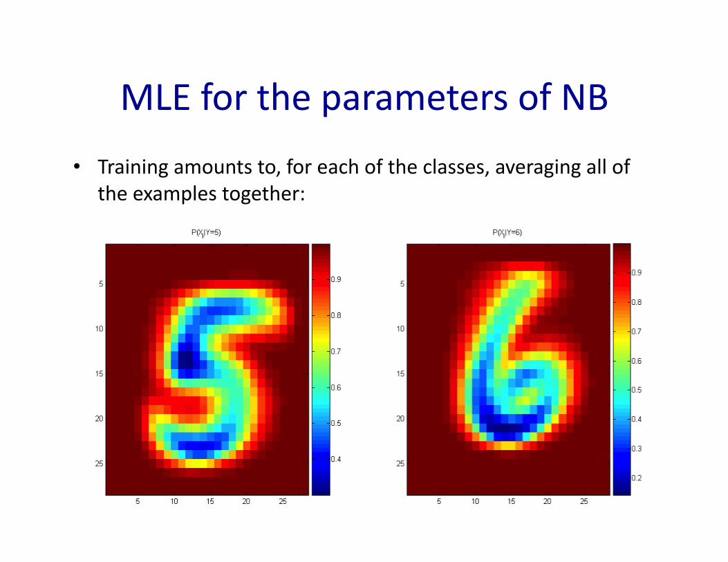
MLEfortheparametersofNB
• Trainingamountsto,foreachoftheclasses,averagingalloftheexamplestogether:
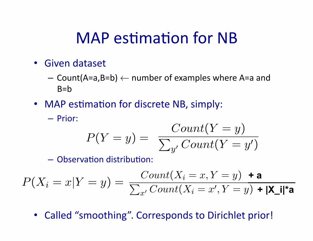
MAPesImaIonforNB• Givendataset
– Count(A=a,B=b)ÃnumberofexampleswhereA=aandB=b
• MAPesImaIonfordiscreteNB,simply:– Prior:
– ObservaIondistribuIon:
• Called“smoothing”.CorrespondstoDirichletprior!
µMLE ,⇥MLE = argmaxµ,�
P (D | µ,⇥)
= �NX
i=1
(xi � µ)
⇥2= 0
= �NX
i=1
xi +Nµ = 0
= �N
⇥+
NX
i=1
(xi � µ)2
⇥3= 0
argmaxwln
✓1
⇥⇥2�
◆N
+NX
j=1
�[tj �P
iwihi(xj)]2
2⇥2
= argmaxw
NX
j=1
�[tj �P
iwihi(xj)]2
2⇥2
= argminw
NX
j=1
[tj �X
i
wihi(xj)]2
P (Y = y) =Count(Y = y)Py0 Count(Y = y�)
2
µMLE ,⇥MLE = argmaxµ,�
P (D | µ,⇥)
= �NX
i=1
(xi � µ)
⇥2= 0
= �NX
i=1
xi +Nµ = 0
= �N
⇥+
NX
i=1
(xi � µ)2
⇥3= 0
argmaxwln
✓1
⇥⇥2�
◆N
+NX
j=1
�[tj �P
iwihi(xj)]2
2⇥2
= argmaxw
NX
j=1
�[tj �P
iwihi(xj)]2
2⇥2
= argminw
NX
j=1
[tj �X
i
wihi(xj)]2
P (Y = y) =Count(Y = y)Py0 Count(Y = y�)
2
µMLE ,⇥MLE = argmaxµ,�
P (D | µ,⇥)
= �NX
i=1
(xi � µ)
⇥2= 0
= �NX
i=1
xi +Nµ = 0
= �N
⇥+
NX
i=1
(xi � µ)2
⇥3= 0
argmaxwln
✓1
⇥⇥2�
◆N
+NX
j=1
�[tj �P
iwihi(xj)]2
2⇥2
= argmaxw
NX
j=1
�[tj �P
iwihi(xj)]2
2⇥2
= argminw
NX
j=1
[tj �X
i
wihi(xj)]2
P (Y = y) =Count(Y = y)Py0 Count(Y = y�)
P (Xi = x|Y = y) =Count(Xi = x, Y = y)Px0 Count(Xi = x�, Y = y)
2
+ a + |X_i|*a