Intra-Industry Trade, Imperfect Competition, Trade Integration and Invasive Species Risk

Anh T. Tu

John Beghin

Iowa State University

This draft May 1, 2004

Preliminary draft not for quotation

Abstract: We analyze the linkage between protectionism and invasive species hazard in the

context of imperfect competition, two-way trade, and multilateral trade liberalization, three

major actual features of agricultural trade and policies in the real world. We revisit the

reciprocal-dumping model with differentiated products, adding trade and agricultural policies

into the framework in the presence of invasive-species risk associated with agriculture. We look

at joint reduction of agricultural tariffs. This type of trade integration is much more likely to

increase the damage from invasive species than predicted by unilateral trade liberalization under

the classical HOS framework. We document the non-monotonic relationship between policy

(trade barriers and farm subsidies) and the expected damages from invasive species. We illustrate

our analytical results with a stylized model of the world wheat market.

0

Intra-Industry Trade, Imperfect Competition, Trade Integration and Invasive Species Risk

1. Introduction

The links between international trade and the environment, are multiple, complex and have been

a topic of continuing heated debate (Copeland and Taylor; Beghin, Roland-Holst, and van der

Mensbrugghe). International trade can be an important driver of environmental change. In the

1990s a related literature has emerged on the interface between trade and sanitary and phyto

sanitary (SPS) issues (see Beghin and Bureau for a review). A more recent literature is emerging

at the triple interface of trade, the environment and SPS issues, namely on trade and invasive

species (IS), with a focus on accidental introductions of exotic species like pests, weeds, and

viruses, by way of trade (Perrings, Williamson and Dalmazzone; Mumford). The trade-SPS-

environment interface is almost inherent to the economics of IS since trade is a major vector of

propagation of these species, although it is not the only one.1 Many papers in this new literature

are focused on the “right” criteria to use or the optimal environmental policy response to the

hazard of IS (Sumner; Binder) and around quarantine as a legitimate policy response to phyto-

sanitary risk (Cook and Frazer; Anderson et al.). Our paper contributes to this new literature on

trade and IS risk in the specific context of agricultural markets and trade.

Agricultural imports have always been an important conduit for biological invasions

(CABI). Despite of the Uruguay Round Agreement of the WTO, protection remains high in

agriculture and its reduction in future trade agreements will influence agricultural trade patterns

and associated IS damages. Elucidating the impact of the structure of agricultural protection on

IS hazards and damages is an important question. In a standard one-way trade Hechsher-Ohlin-

Samuelson (HOS) model, Costello and McAusland show that lowering agricultural tariffs could

lower the damage from exotic species, even though the volume of trade rises and the rate of IS 1 “Natural” invasions occur because of natural vectors (weather related ones, animal migration).

1

introduction rises, because an increase in imports results in a reduced domestic agricultural

output. Thus the crop volume susceptible and available for damage and the land area potentially

affected by the pest are reduced, hence damages can be reduced as well leading to an ambiguous

effect of trade on IS damages.

Our paper builds upon the enquiry of Costello and McAusland. We make major

departures by analyzing the linkage between protectionism and damages from IS in the context

of imperfect competition, two-way trade and multilateral trade liberalization. Intra-industry trade

and imperfect competition characterize agricultural trade patterns in the real world. For example,

wheat trade is oligopolistic and wheat is a differentiated commodity with most countries

importing and exporting wheat (See Table 1). Two-way trade patterns hold even more for more

broadly defined commodities such as coarse grains as shown in table 2. The HOS framework has

limited empirical relevance in this context.

We also depart with the previous analysis by considering multilateral trade liberalization.

Trade integration occurs mostly through multilateral or regional agreements (e.g., The Uruguay

Round of the WTO, NAFTA). Seldom do countries engage in unilateral trade liberalization but

rather commit to jointly reduce their protection through regional or multilateral agreements.2

Another argument to consider joint reforms is that transaction costs have been falling for both

exports and imports through cheaper transportation, cheaper refrigeration and insurance, etc.

Joint tariff reduction mimics the joint lowering of transaction costs on both sides of any border.

We revisit the reciprocal dumping model considering differentiated products and adding

trade into the framework. We consider joint tariff reductions and their effect on expected IS

damage. We find that this type of trade integration is much more likely to increase expected

2 There are exceptions such as New Zealand’s unilateral trade liberalization in the 1980s but by and large joint reforms are much more common (Bhagwati).

2

damage from exotic species in our two-way trade model, as compared to unilateral liberalization

and on-way trade. Hence the unexpected ambiguity of Costello and McAusland is much reduced

in with our more realistic setup.

Domestic farm subsidies are another consideration. Agriculture in OECD countries is

characterized by heavy subsidies which have to some extent, substituted for the lower border

protection (OECD). Since 1996 these subsidies have been slowly reduced as part of the Uruguay

Round Agreement on Agriculture (URAA). The current Doha round is also considering sharper

reductions in production subsidies in agriculture. We incorporate this second-best dimension of

domestic subsidies in our analysis of trade integration and their role on IS risk introduction and

damages. We document the non-monotonic relationship between protection structure (border and

domestic policies) and damages from exotic species introduction. We focus on the key role of

domestic subsidies and their reform to either increase or decrease IS introduction and damage.

The remainder of the paper is organized as follows. The trade model is presented next.

Section 3 models the IS introduction. Then the linkage between trade reform and IS introduction

is then established. We illustrate and examine the robustness of the results in section 5 by

calibrating the analytical model to recent data on wheat trade and the associated damages from

exotic species. Summary remarks then conclude the paper.

2. A segmented-market model with differentiated product

Assume that there are two countries, Home and Foreign, and that each country has one firm

producing commodity Z. Assume that each firm regards each country as a separate market and

therefore chooses the profit-maximizing quantity for each country separately by making price

discrimination of the third degree. The Home firm produces output x for domestic consumption

3

and output x* for Foreign consumption. Similarly, the Foreign firm produces output y for export

to Home, and output y* for its own market. The idea was first proposed by Brander (1981) and

elaborated by Brander and Krugman (1983).

Assume that Home good and Foreign good are imperfect substitutes in each market such

that the Home demands for domestic good and imports are

(1) ( , )x y x x x yx p p a b p kp= − + , and

(2) ( , )x y y y yy p p a b p kp= − + x

)

,

where are price of Home and Foreign goods in the Home market. All parameters are

assumed to be positive and so is expression

( ,X Yp p

xb b k− 2y by integrability of a demand system derived

by maximizing a quasi-linear utility under budget constraint (see appendix 1).

Similarly, Foreign demands for its own domestic good and the imports are

(3) * * * * ***( , )x y y y y xy p p a b p kp= − + , and

(4) * * * * ***( , )x y x x x yx p p a b p kp= − + .

Again, all parameters are assumed to be positive and so is expression . *xb b k− 2y*

Assume that Home and Foreign governments impose tariffs on imports ( , *)τ τ and

subsidize their production ( with subsidies being proportional to their unit cost, c. Tariffs

and subsidies are expressed in ad valorem rate. Home and Foreign firm’ problems are

), *s s

(5) [ ] ( ) ( )*

* * *

. . .{ , }( , , ) (1 ) , (1 ) (1 ) * (1 *),

x xx x y x x y

w r t p pMax p s p c s x p p p c s x p p FCπ τ τ τ⎡ ⎤= − − + + − − + −⎣ ⎦

rr , and

(6) ( ) ( )*

* * *

. . .{ , }*( , , *) (1 *) , (1 ) (1 *) * (1 *), *

y yy x y y x y

w r t p pMax p s p c s y p p p c s y p p FCπ τ τ τ⎡ ⎤⎡ ⎤= − − + + − − + −⎣ ⎦ ⎣ ⎦

rr ,

respectively, where * *( , , , )x x y yp p p p p=r , ( , *)τ τ τ=

r , and FC and FC* are fixed costs of the Home

and Foreign firm. This setting is similar to the “reciprocal dumping” model of Brander and

4

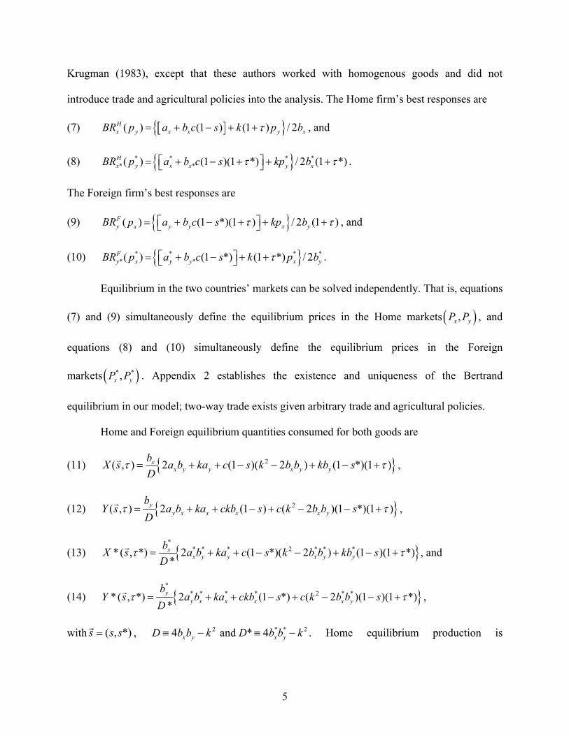
Krugman (1983), except that these authors worked with homogenous goods and did not

introduce trade and agricultural policies into the analysis. The Home firm’s best responses are

(7) [ ]{ }( ) (1 ) (1 ) / 2Hx y x x y xBR p a b c s k p bτ= + − + + , and

(8) { }* * * ** *( ) (1 )(1 *) / 2 (1 *H

x y x x y xBR p a b c s kp b )τ τ⎡ ⎤= + − + + +⎣ ⎦ .

The Foreign firm’s best responses are

(9) { }( ) (1 *)(1 ) / 2 (1 )Fy x y y x yBR p a b c s kp bτ τ⎡ ⎤= + − + + +⎣ ⎦ , and

(10) { }* * ** *( ) (1 *) (1 *) / 2F

y x y y x*yBR p a b c s k p bτ⎡ ⎤= + − + +⎣ ⎦ .

Equilibrium in the two countries’ markets can be solved independently. That is, equations

(7) and (9) simultaneously define the equilibrium prices in the Home markets ( , )x yP P , and

equations (8) and (10) simultaneously define the equilibrium prices in the Foreign

markets ( * *, )x yP P . Appendix 2 establishes the existence and uniqueness of the Bertrand

equilibrium in our model; two-way trade exists given arbitrary trade and agricultural policies.

Home and Foreign equilibrium quantities consumed for both goods are

(11) { }2( , ) 2 (1 )( 2 ) (1 *)(1 )xx y y x y y

bX s a b ka c s k b b kb sD

τ τ= + + − − + − +r ,

(12) { }2( , ) 2 (1 ) ( 2 )(1 *)(1 )yy x x x x y

bY s a b ka ckb s c k b b s

Dτ τ= + + − + − − +

r ,

(13) { }*

* * * 2 * * ** ( , *) 2 (1 *)( 2 ) (1 )(1 *)*

xx y y x y y

bX s a b ka c s k b b kb sD

τ τ= + + − − + − +r , and

(14) { }*

* * * * 2 * ** ( , *) 2 (1 *) ( 2 )(1 )(1 *)*

yy x x x x y

bY s a b ka ckb s c k b b s

Dτ τ= + + − + − − +

r ,

with , . Home equilibrium production is ( , *)s s s=r 2 *4 and * 4x y x yD b b k D b b k≡ − ≡ −* 2

5

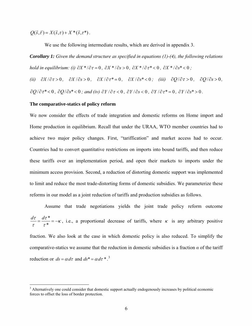
( , ) ( , ) *( , *)Q s X s X sτ τ τ= +rr r r .

We use the following intermediate results, which are derived in appendix 3.

Corollary 1: Given the demand structure as specified in equations (1)-(4), the following relations

hold in equilibrium: (i) * / 0X τ∂ ∂ = , * / 0X s∂ ∂ > , * / * 0X τ∂ ∂ < , * / * 0X s∂ ∂ < ;

(ii) / 0X τ∂ ∂ > , , / 0X s∂ ∂ > / * 0X τ∂ ∂ = , / * 0X s∂ ∂ < ; (iii) / 0Q τ∂ ∂ > , , / 0Q s∂ ∂ >

/ * 0Q τ∂ ∂ < , ; and (iv) / * 0Q s∂ ∂ < / 0Y τ∂ ∂ < , / 0Y s∂ ∂ < , / * 0Y τ∂ ∂ = , . / * 0Y s∂ ∂ >

The comparative-statics of policy reform

We now consider the effects of trade integration and domestic reforms on Home import and

Home production in equilibrium. Recall that under the URAA, WTO member countries had to

achieve two major policy changes. First, “tariffication” and market access had to occur.

Countries had to convert quantitative restrictions on imports into bound tariffs, and then reduce

these tariffs over an implementation period, and open their markets to imports under the

minimum access provision. Second, a reduction of distorting domestic support was implemented

to limit and reduce the most trade-distorting forms of domestic subsidies. We parameterize these

reforms in our model as a joint reduction of tariffs and production subsidies as follows.

Assume that trade negotiations yields the joint trade policy reform outcome

**

d dτ τ κτ τ

= = − , i.e., a proportional decrease of tariffs, where κ is any arbitrary positive

fraction. We also look at the case in which domestic policy is also reduced. To simplify the

comparative-statics we assume that the reduction in domestic subsidies is a fraction α of the tariff

reduction or and * *ds d ds dα τ α= = τ

.3

3 Alternatively one could consider that domestic support actually endogenously increases by political economic forces to offset the loss of border protection.

6

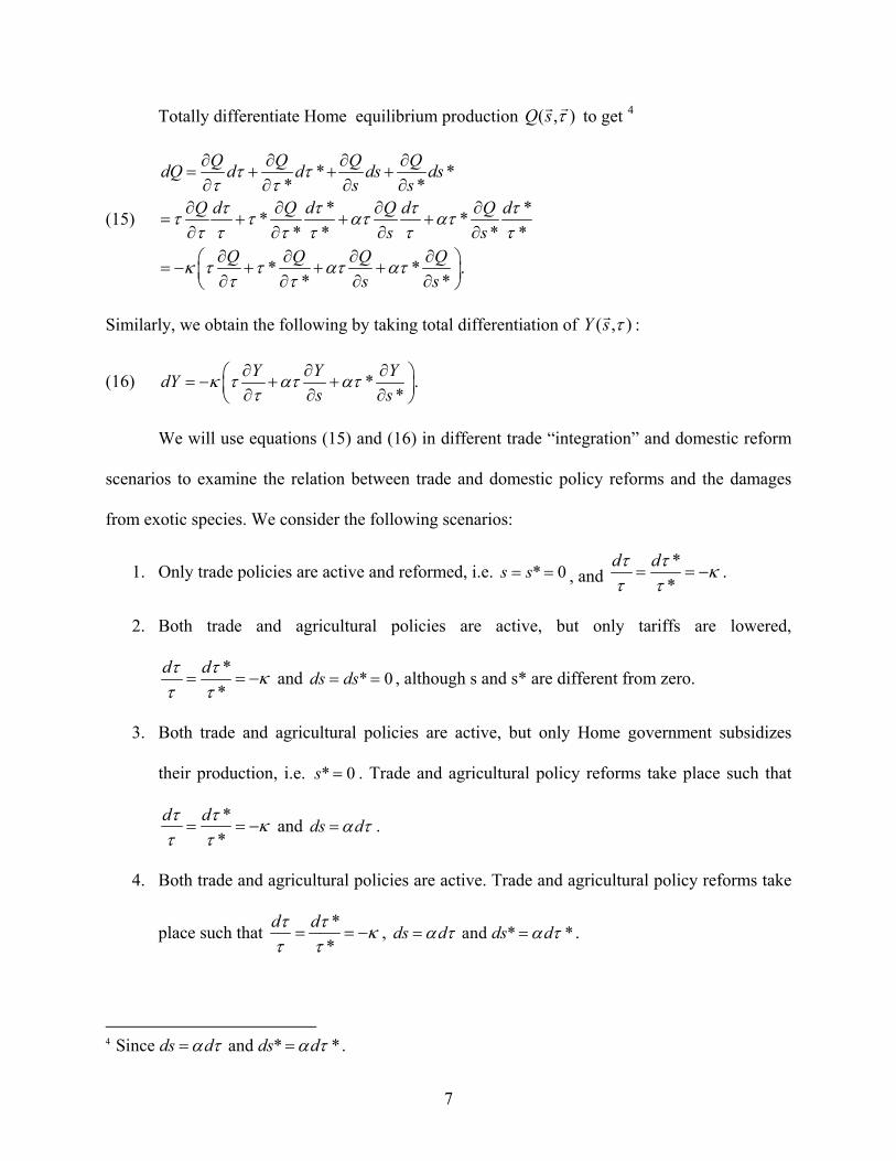
Totally differentiate Home equilibrium production ( , )Q s τrr to get 4

(15)

* ** *

* ** ** * * *

* * .* *

Q Q Q QdQ d d ds dss s

Q d Q d Q d Q ds s

Q Q Q Qs s

τ ττ ττ τ ττ τ ατ ατ τ

τ τ τ τ τ τ

κ τ τ ατ αττ τ

∂ ∂ ∂ ∂= + + +∂ ∂ ∂ ∂

∂ ∂ ∂ ∂= + + +

∂ ∂ ∂ ∂∂ ∂ ∂ ∂ ⎞⎛= − + + +⎜ ⎟∂ ∂ ∂ ∂⎝ ⎠

Similarly, we obtain the following by taking total differentiation of ( , )Y s τr :

(16) * .*

Y Y YdYs s

κ τ ατ αττ

∂ ∂ ∂ ⎞⎛= − + +⎜ ⎟∂ ∂ ∂⎝ ⎠

We will use equations (15) and (16) in different trade “integration” and domestic reform

scenarios to examine the relation between trade and domestic policy reforms and the damages

from exotic species. We consider the following scenarios:

1. Only trade policies are active and reformed, i.e. * 0s s= = , and *

*d dτ τ κτ τ

= = − .

2. Both trade and agricultural policies are active, but only tariffs are lowered,

**

d dτ τ κτ τ

= = − and , although s and s* are different from zero. * 0ds ds= =

3. Both trade and agricultural policies are active, but only Home government subsidizes

their production, i.e. . Trade and agricultural policy reforms take place such that * 0s =

**

d dτ τ κτ τ

= = − and ds dα τ= .

4. Both trade and agricultural policies are active. Trade and agricultural policy reforms take

place such that **

d dτ τ κτ τ

= = − , and * *ds d ds dα τ α τ= = .

4 Since and * *.ds d ds dα τ α= = τ

7

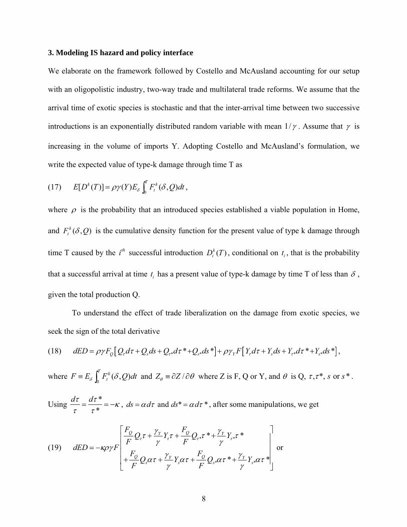
3. Modeling IS hazard and policy interface

We elaborate on the framework followed by Costello and McAusland accounting for our setup

with an oligopolistic industry, two-way trade and multilateral trade reforms. We assume that the

arrival time of exotic species is stochastic and that the inter-arrival time between two successive

introductions is an exponentially distributed random variable with mean 1/γ . Assume that γ is

increasing in the volume of imports Y. Adopting Costello and McAusland’s formulation, we

write the expected value of type-k damage through time T as

(17) , 0

[ ( )] ( ) ( , )Tk k

tE D T Y E F Q dtδργ δ= ∫

where ρ is the probability that an introduced species established a viable population in Home,

and ( , )ktF Qδ is the cumulative density function for the present value of type k damage through

time T caused by the successful introduction , conditional on , that is the probability

that a successful arrival at time has a present value of type-k damage by time T of less than

thi ( )kiD T it

it δ ,

given the total production Q.

To understand the effect of trade liberalization on the damage from exotic species, we

seek the sign of the total derivative

(18) [ ] [ ]* * * ** * *Q s s Y s sdED F Q d Q ds Q d Q ds F Y d Y ds Y d Y dsτ τ τ τργ τ τ ργ τ τ= + + + + + + + * ,

where and 0

( , )T k

tF E F Q dtδ δ≡ ∫ /Z Zθ θ≡ ∂ ∂ where Z is F, Q or Y, and θ is Q, , *, or *s sτ τ .

Using **

d dτ τ κτ τ

= = − , and * *ds d ds dα τ α= = τ , after some manipulations, we get

(19) * *

* *

* *

* *

Q QY Y

Q QY Ys s s s

F FQ Y Q Y

F FdED F

F FQ Y Q Y

F F

τ τ τ τγ γτ τ τ τγ γ

κργγ γατ ατ ατ ατγ γ

⎡ ⎤+ + +⎢ ⎥

⎢ ⎥= −⎢ ⎥+ + + +⎢ ⎥⎣ ⎦

or

8

, * *

* *( ) / ( )

Q QY Y

Q Qs s s sY Y

F FQ Y Q Y

F FQ Y Q YF

s s

τ τ τ τγ γ

γ γ

ε ε ε ε ε ε ε εκργ

ε ε ε ε ατ ε ε ε ε ατ

⎡ ⎤+ + += − ⎢ ⎥

+ + + +⎢ ⎥⎣ ⎦* / *

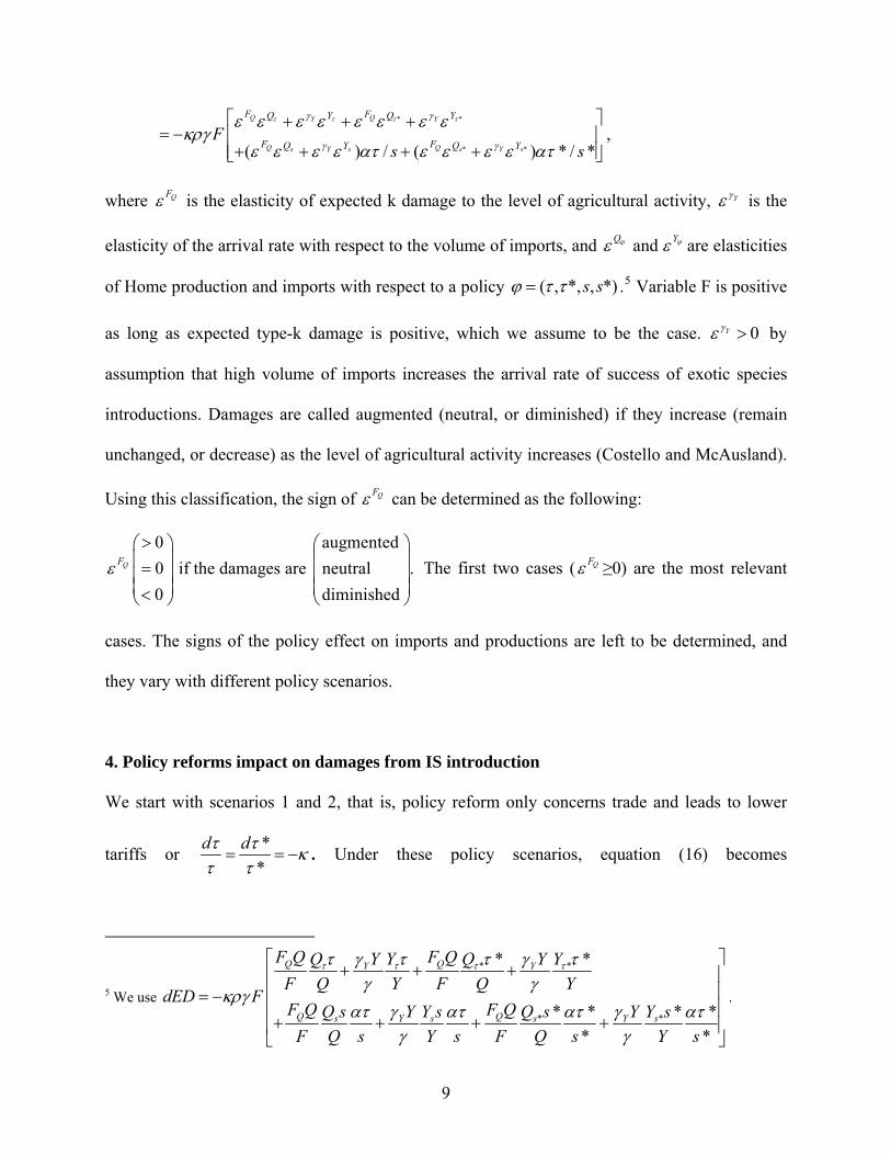
where QFε is the elasticity of expected k damage to the level of agricultural activity, Yγε is the

elasticity of the arrival rate with respect to the volume of imports, and and Q Yϕ ϕε ε are elasticities

of Home production and imports with respect to a policy ( , *, , *)s sϕ τ τ= .5 Variable F is positive

as long as expected type-k damage is positive, which we assume to be the case. by

assumption that high volume of imports increases the arrival rate of success of exotic species

introductions. Damages are called augmented (neutral, or diminished) if they increase (remain

unchanged, or decrease) as the level of agricultural activity increases (Costello and McAusland).

Using this classification, the sign of

0Yγε >

QFε can be determined as the following:

0 augmented0 if the damages are neutral .0 diminished

QFε> ⎞ ⎞⎛ ⎛

⎟⎜ ⎜= ⎟⎜ ⎜⎜ ⎟ ⎜ ⎟<⎝ ⎝

⎟⎟

⎠ ⎠

The first two cases ( QFε ≥0) are the most relevant

cases. The signs of the policy effect on imports and productions are left to be determined, and

they vary with different policy scenarios.

4. Policy reforms impact on damages from IS introduction

We start with scenarios 1 and 2, that is, policy reform only concerns trade and leads to lower

tariffs or **

d dτ τ κτ τ

= = − . Under these policy scenarios, equation (16) becomes

5 We use

* *

* *

* *

* * * ** *

Q QY Y

Q Qs Y s s Y s

F Q F QQ Y Y Q Y YF Q Y F Q Y

dED FF Q F QQ s Y Y s Q s Y Y s

F Q s Y s F Q s Y s

τ τ τ ττ γ τ τ γ τγ γ

κργατ γ ατ ατ γ ατ

γ γ

⎡ ⎤+ + +⎢ ⎥

⎢ ⎥= −⎢ ⎥+ + + +⎢ ⎥⎣ ⎦

.

9

**

Y YdY κ τ ττ τ∂ ∂⎛ ⎞= − +⎜ ⎟∂ ∂⎝ ⎠

.

Proposition 1: Given the demand structure (1)-(4), a joint tariff reduction without domestic

policy reform increases the rate of successful IS introduction to Home.

Proof: See Appendix 4.

The proposition points out the straightforward relation between trade integration and the rate of

successful introductions of IS. Trade integration via multilateral trade liberalization increases

imports, hence the platform for IS introduction. One should however, remember that not all

successful introductions cause damages, and that the extent of damages is endogenous. The

correlation between trade liberalization and damages caused by exotic species is represented by

equation (19) under scenario 1, or * *Q QY YF FQ Y Q YdED F τ τ τγ γκργ ε ε ε ε ε ε ε ε τ⎡ ⎤= − + + +⎣ ⎦ .

Hence, the expected change in damages has four components corresponding to the two policy

types (tariffs, production subsidies), and the two vectors (production, imports).

Proposition 2: Given the demand structure (1)-(4), a joint tariff reduction without domestic

policy reform increases

does not affectdecreases

⎞⎛⎟⎜⎟⎜

⎜ ⎟⎝ ⎠

the expected damages if and only if

(20) *( )Q

Y

FQ Qτ τ τγ

γ

ε ε ε εε

<+ −

>.

Proof: The proposition follows directly from applying elements of corollary 1 to equation (19).

QED.

To provide intuition, we compare the IS damages induced by the trade reform in our imperfect-

competition and two-way trade setup to the outcome in the one-way trade cum unilateral reform

case. The “one-way trade” context can be interpreted in our framework as when the Home firm’s

10

export X* does not exist.6 Therefore, the demand system is characterized only by equations (1),

(2) and (4). A Bertrand equilibrium exists and is unique in this “one-way trade” version of the

model (See appendix 5). As a result, the relation between trade reform and the damages from the

exotic species in the one-way trade model is characterized by equation (20) but with *Qτε =0.

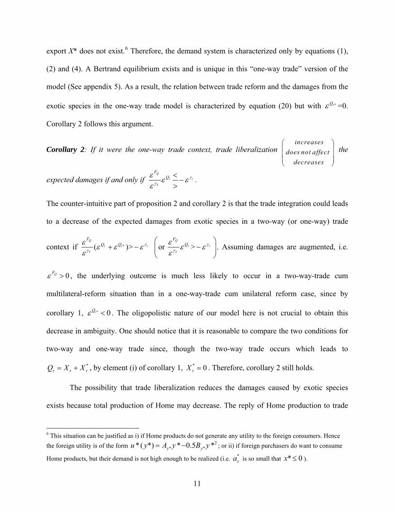
Corollary 2 follows this argument.

Corollary 2: If it were the one-way trade context, trade liberalization increases

does not affectdecreases

⎞⎛⎟⎜⎟⎜

⎜ ⎟⎝ ⎠

the

expected damages if and only if Q

Y

FQτ τγ

γ

ε ε εε

<−

>.

The counter-intuitive part of proposition 2 and corollary 2 is that the trade integration could leads

to a decrease of the expected damages from exotic species in a two-way (or one-way) trade

context if *( )>Q

Y

FQ Qτ τ τγ

γ

ε ε ε εε

+ − or >Q

Y

FQτ γ

γ

ετε ε

ε⎞⎛

− ⎟⎜⎝ ⎠

. Assuming damages are augmented, i.e.

, the underlying outcome is much less likely to occur in a two-way-trade cum

multilateral-reform situation than in a one-way-trade cum unilateral reform case, since by

corollary 1, . The oligopolistic nature of our model here is not crucial to obtain this

decrease in ambiguity. One should notice that it is reasonable to compare the two conditions for

two-way and one-way trade since, though the two-way trade occurs which leads to

0QFε >

* 0Qτε <

*Q X Xτ τ= + τ , by element (i) of corollary 1, * 0Xτ = . Therefore, corollary 2 still holds.

The possibility that trade liberalization reduces the damages caused by exotic species

exists because total production of Home may decrease. The reply of Home production to trade

6 This situation can be justified as i) if Home products do not generate any utility to the foreign consumers. Hence the foreign utility is of the form ; or ii) if foreign purchasers do want to consume

Home products, but their demand is not high enough to be realized (i.e.

2* ** ( *) * 0.5 *y yu y A y B y= −

*xa is so small that ). * 0x ≤

11

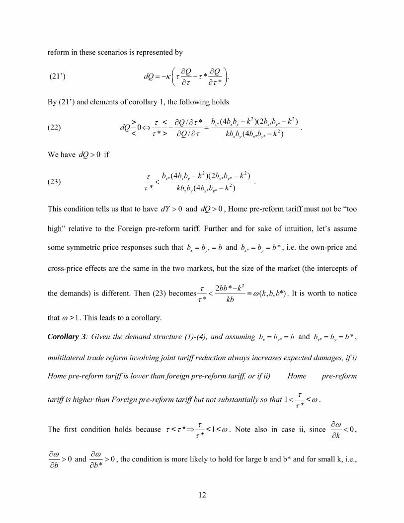
reform in these scenarios is represented by

(21’) **

Q QdQ κ τ ττ τ

∂ ∂⎛ ⎞= − +⎜ ⎟∂ ∂⎝ ⎠.

By (21’) and elements of corollary 1, the following holds

(22) 2 2

* *2

* *

(4 )(2 )/ *0* / (4 )

x x y x y

x y x y

b b b k b b kQdQQ kb b b b k

τ ττ τ

− −∂ ∂⇔ − =

∂ ∂ −> << >

* .

We have if 0dQ >

(23) 2 2

* *2

* *

(4 )(2 )* (4

x x y x y

x y x y

b b b k b b kkb b b b k

ττ

− −<

−*

)

b

.

This condition tells us that to have and , Home pre-reform tariff must not be “too

high” relative to the Foreign pre-reform tariff. Further and for sake of intuition, let’s assume

some symmetric price responses such that

0dY > 0dQ >

*x yb b= = and * *x yb b b= = , i.e. the own-price and

cross-price effects are the same in the two markets, but the size of the market (the intercepts of

the demands) is different. Then (23) becomes22 * ( , , *)

*bb k k b b

kbτ ωτ

−< ≡ . It is worth to notice

that 1ω > . This leads to a corollary.

Corollary 3: Given the demand structure (1)-(4), and assuming *x yb b b= = and ,

multilateral trade reform involving joint tariff reduction always increases expected damages, if i)

Home pre-reform tariff is lower than foreign pre-reform tariff, or if ii) Home pre-reform

tariff is higher than Foreign pre-reform tariff but not substantially so that

* *x yb b b= =

1 τ ωτ

< <*

.

The first condition holds because 1ττ ττ

⇒< * < <*

ω . Note also in case ii, since 0kω∂<

∂,

0bω∂>

∂ and 0

*bω∂

>∂

, the condition is more likely to hold for large b and b* and for small k, i.e.,

12

for large own-price effects and/or for small degree of substitution between foreign and home

goods. This corollary suggests that a relatively open country liberalizing its trade with a more

protectionist partner will face increase expected damages, other things being equal.

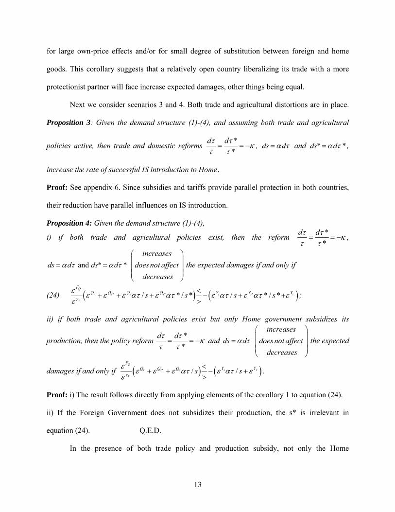
Next we consider scenarios 3 and 4. Both trade and agricultural distortions are in place.

Proposition 3: Given the demand structure (1)-(4), and assuming both trade and agricultural

policies active, then trade and domestic reforms **

d dτ τ κτ τ

= = − , ds dα τ= and * *ds dα τ= ,

increase the rate of successful IS introduction to Home.

Proof: See appendix 6. Since subsidies and tariffs provide parallel protection in both countries,

their reduction have parallel influences on IS introduction.

Proposition 4: Given the demand structure (1)-(4),

i) if both trade and agricultural policies exist, then the reform **

d dτ τ κτ τ

= = − ,

and * *ds d ds dα τ α τ= =increases

does not affectdecreases

⎞⎛⎟⎜⎟⎜

⎜ ⎟⎝ ⎠

the expected damages if and only if

(24) ( ) ( )* * */ * / * / * / *Q

s s s s

Y

FQ Q Q Q Y Y Ys s s sτ τ τ

γ

ε ε ε ε ατ ε ατ ε ατ ε ατ εε

<+ + + − + +

>;

ii) if both trade and agricultural policies exist but only Home government subsidizes its

production, then the policy reform **

d dτ τ κτ τ

= = − and ds dα τ= increases

does not affectdecreases

⎞⎛⎟⎜⎟⎜

⎜ ⎟⎝ ⎠

the expected

damages if and only if ( ) ( )* / /Q

s s

Y

FQ Q Q Y Ys sτ τ τ

γ

ε ε ε ε ατ ε ατ εε

<+ + − +

>.

Proof: i) The result follows directly from applying elements of the corollary 1 to equation (24).

ii) If the Foreign Government does not subsidizes their production, the s* is irrelevant in

equation (24). Q.E.D.

In the presence of both trade policy and production subsidy, not only the Home

13

production’s reply to trade reform is non-monotonic, but also is the Home’s imports. The non-

monotonicity of production in this case can be seen by expressing (15) in terms of elasticity,

which leads to

(25) * **0*

s sQ Q Q QdQs s

τ ττ τε ε α ε ε ⎞⎛⇔ + − +⎜ ⎟⎝ ⎠

> << >

.

There are large and increasing differences in the levels of support and market protection among

OECD countries, reflecting different historical uses of policy instruments, and the varying pace

and degree of progress in agricultural policy reform. For the 2000-02 period, the average PSE

was below 5% in Australia and New Zealand, below 25% for the United States, 35% in the

European Union and around 60% for Japan, Korea among others (figure 2). Support to

Australian agriculture, for example, is extremely low and domestic producer prices, which were

on average 5% higher than world price in the mid-1980s, have been broadly aligned with world

prices since 2001 (OECD, 2003, page 120). Proposition 4(i) can refer to the trade activities

between the US and EU or Japan, while US-Australia or US-New Zealand exchange could be the

case in proposition 4(ii).

5. Calibration of the wheat model in the presence of IS

Wheat provides an excellent opportunity to illustrate our analytical results. Wheat trade can be a

major vector of IS (CABI), and as mentioned before wheat is differentiated and its trade is

oligopolistic. Table 1 summarizes the bilateral trade on wheat between the US, the European

Union 15 (EU), Canada and the “rest of the world” in the marketing year of July 2001-June

2002. There is a large two-way trade between the US and Canada: 98% of US wheat imports

come from Canada, while 25% of Canada wheat imports are from the US. In total, EU’s total

wheat imports are almost as large as its total wheat exports. Therefore, to illustrate the theoretical

14

findings in the previous sections, we calibrate the model using data on wheat production and

trade and on invasive species associated with wheat for the four-country case (the US, the EU,

Canada, and the rest of the world (ROW)).

Table 3 indicates the summary policy distortions at the border and farm subsidies for

major players in the wheat market for 2001 using OECD and WITS data. As noted by Mitchell

and Mielke, despite these significant achievements in improved rules for trade with the URAA,

the amount of trade liberalization achieved in wheat was modest because of the way these

reforms were done. Many countries applied the Uruguay Round provisions so that they could

protect producers in key sectors from foreign competition. Applied tariffs were often set high

and bound tariffs were often set even higher which leaves open the possibility of future increases

in applied tariffs. Wheat export subsides have been largely eliminated, but the possibility they

could be resumed remains. Implementation of minimum access and tariff reduction has also met

with problems as countries have introduced new measures to offset agreed reforms.

While trade barrier has the tendency to reduce, the domestic policies still support and

protect the agriculture activities. In 2002, for the OECD countries, the level of support to

producers stabilized, but with a slight increase in protection and a slight reduction in market

orientation. Support to producers for the OECD as a whole, as measure by the %PSE, remained

unchanged at 31% in 2002 compared to 2001 (Figure 1, OECD 2003). For the three-year period

2000-2002, the %PSE averaged 31% compared with the 1986-88 average of 38%. In output-

linked support, the nominal rate of protection, as measure by the producer nominal assistance

coefficients increased slightly with average producer prices 31% above the world price in 2002

compared to 30% in 2001.

Output-linked support reduces the transmission of world price changes to producers and

15

thus dampens the influence of world market price changes on domestic production decisions.

Over the long-term market protection has decreased as prices in domestic markets were, on

average, 57% higher in 1986-88. The nominal assistance coefficient for the whole OECD, as

measured by the producer NAC, also slightly increased in 2002 compared to 2001 indicating a

slight reduction in market orientation. Total farm receipt in 2000-02 were on average 46% higher

than they would have be if entirely generated in markets without any support, while they were

61% higher in 1986-88. This is an indicator of an improvement in market orientation in terms of

greater share of farm receipts generated in markets than created by government intervention.

Structure of the wheat model:

Equations (1) to (4) specified in the previous section are calibrated to 2001/2 data. To account

for damages we decompose output into a land component and a yield component. Damages are

expressed as production losses via decreased yield. This is the way plant pathologists model the

impact of pest on crops (CABI). We calibrate the four-country model, which are the US, the EU,

Canada and the rest of the world (ROW), with a vector of exports and imports for each country

since there are several partners for each country. Wheat is assumed to be differentiated, hence we

have 4 kinds of wheat: US wheat, EU wheat, Canada wheat, and wheat produced by the rest of

the world.

The general framework for each country sub-model consists of the following:

Planted area: ( ,i i )iAH f WP AP= ,

Yield: , ( )* (1i iY g WP E YL⎡ ⎤= − ⎣ ⎦)i

iWheat production: , *i iPROD AH Y=

16

where { }, , ,i US EU CAN ROW= , AH is the acreage, WP denotes the real wheat price, AP

represents the real price of alternative crops (corn, barley, oats and rye, etc), Y stands for yield,

YL is the yield loss due to the non-indigenous species and PROD is the wheat production.

The inventory demands are assumed to be constant across the period.

Data for area, yield, production and consumption were gathered from the World Grain

Statistics of the International Grains Council. Price data were obtained from the USDA, Attaché

Reports, AgCanada and the International Grains Councils. The protection data were collected

from the OECD and WITS. Finally, CABI’s Crop Protection Compendium provides most of the

data for the underlying pests. Price responses come from the FAPRI elasticity database.

Damages D of the pest p are expressed in the value of crop losses: ( )i ipE D h E YL⎡ ⎤ ⎡= ⎤⎣ ⎦ ⎣ ⎦ .

Simulated results will be presented at the conference.

17

References

Anderson, K., C. McRae, and D. Wilson, Eds. The Economics of Quarantine and the SPS

Agreement, CIES and AFFA, 2001.

Beghin J., D. Roland-Holst, and D. van der Mensbrugghe, eds. Trade and the Environment in

General Equilibrium. Evidence from Developing Economies, Kluwer Academic

Publishers, Dordrecht, The Netherlands, 2002.

Beghin J., and J.C. Bureau. “Quantitative Policy Analysis of Sanitary, Phytosanitary and

Technical barriers to Trade,” Economie Internationale 87(2001): 107-130.

Copeland, B.R., and M.S. Taylor. Trade, Growth, and the Environment,” Journal of Economic

Literature XLII (2004): 7-71

Ben-Zvi, S. and Helpman, E. “Oligopoly in segmented markets.” In Imperfect Competition and

International Trade, G. M. Grossman Ed. The MIT Press. 31-54, 1992.

Bhagwati, J. ed. Going Alone. The Case for Relaxed Reciprocity in Freeing Trade. Cambridge,

MA: The MIT Press, 2002.

Binder, M. “The Role of Risk and Cost Benefit Analysis in Determining Quarantine measures,”

Australia Productivity Commission Staff Research Paper, Canberra, 2002.

Brander, J. “Intraindustry trade in identical commodities,” Journal of International Economics

11 (1981):1-14.

Brander, J. and Krugman, P. R. A “reciprocal dumping” model of international trade. Journal of

International Economics 15 (1983): 313-321.

CABI. 2003. CAB International Crop Protection Compendium. CDrom. CABI, Wallingford, UK.

Cook, D.C., and R.W. Fraser. “Exploring the regional Implications of interstate quarantine

policies in Western Australia,” Food Policy 27 (2002): 143-157.

18

Costello, C. and McAuland,C. Protectionism, Trade, and Measures of Damage from Exotic

Species Introductions. American Journal of Agricultural Economics 85(4) (2003): 964-

975.

Mitchell, D. and M. Mielke. “The Global Wheat Market: Policies and Priorities”. in D. Aksoy,

M. A. and J. Beghin, eds. Global Agricultural Trade and the Developing Countries.

Oxford University Press and The World Bank, forthcoming.

Mumford,J.D. (2002), Economic Issues Related to Quarantine in International Trade, European

Review of Agricultural Economics 29: 329-48.

OECD. Agricultural policies in OECD Countries. Monitoring and Evaluation 2003. OECD

publications, Paris, 2003.

Perrings, C., M.Williamson, and S. Dalmazzone (eds), 2000, The economics of biological

invasions. Edward Elgar Publishing, Cheltenham, UK.

Perrings, C., M.Williamson, E.B. Barbier, D. Delfino, S. Dalmazzone, J.F. Shogren, P.J.

Simmons, and A.R.Watkinson (2002). “ Biological Invasion Risks and the Public Good:

an Economic Perspective,” Conservation Ecology 6.

Sumner, D. ed. Exotic Pest and Diseases: Biology, Economics, and Public Policy for

Biosecurity, Iowa State press, 2004.

19

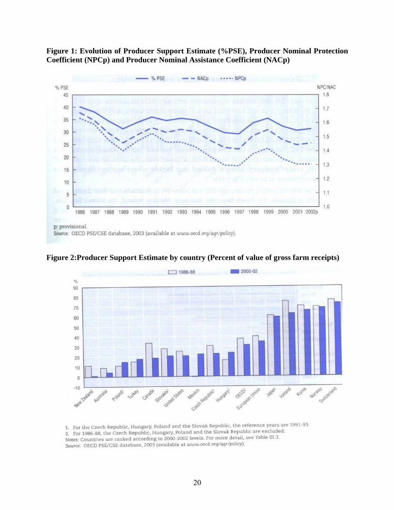
Figure 1: Evolution of Producer Support Estimate (%PSE), Producer Nominal Protection Coefficient (NPCp) and Producer Nominal Assistance Coefficient (NACp)

Figure 2:Producer Support Estimate by country (Percent of value of gross farm receipts)

20

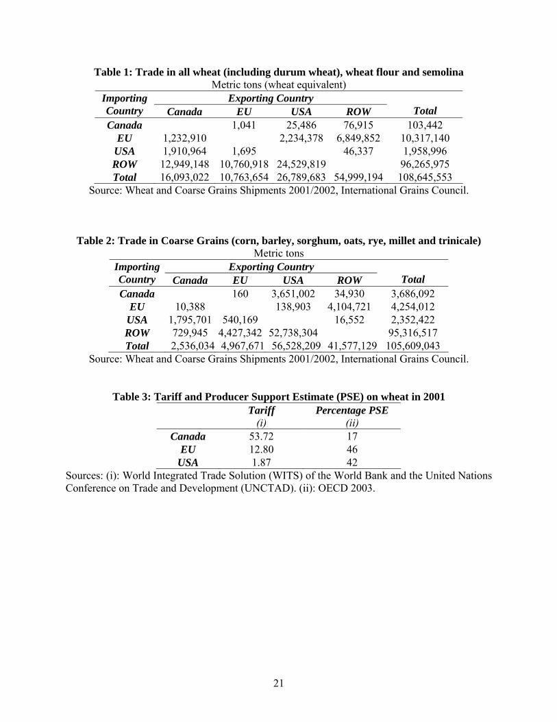
Table 1: Trade in all wheat (including durum wheat), wheat flour and semolina Metric tons (wheat equivalent)

Exporting Country Importing Country Canada EU USA ROW Total Canada 1,041 25,486 76,915 103,442

EU 1,232,910 2,234,378 6,849,852 10,317,140 USA 1,910,964 1,695 46,337 1,958,996 ROW 12,949,148 10,760,918 24,529,819 96,265,975 Total 16,093,022 10,763,654 26,789,683 54,999,194 108,645,553

Source: Wheat and Coarse Grains Shipments 2001/2002, International Grains Council.

Table 2: Trade in Coarse Grains (corn, barley, sorghum, oats, rye, millet and trinicale) Metric tons

Exporting Country Importing Country Canada EU USA ROW Total Canada 160 3,651,002 34,930 3,686,092

EU 10,388 138,903 4,104,721 4,254,012 USA 1,795,701 540,169 16,552 2,352,422 ROW 729,945 4,427,342 52,738,304 95,316,517 Total 2,536,034 4,967,671 56,528,209 41,577,129 105,609,043

Source: Wheat and Coarse Grains Shipments 2001/2002, International Grains Council.

Table 3: Tariff and Producer Support Estimate (PSE) on wheat in 2001

Tariff

(i) Percentage PSE

(ii) Canada 53.72 17

EU 12.80 46 USA 1.87 42

Sources: (i): World Integrated Trade Solution (WITS) of the World Bank and the United Nations Conference on Trade and Development (UNCTAD). (ii): OECD 2003.

21

Appendix Appendix 1: The inverse demands corresponding to equations (1)-(2) are ( , )x x xp x y A B x Ky= − − , and

( , )y y yp x y A B y Kx= − − . All parameters are positive and so is expression 2xB B K−y . This

demand system can be derived by maximizing quasi-linear utility, subject to the budget constraint X YI z p x p y= + + , where I is Home income. The aggregate utility function is of the form ,where z is the aggregate consumption of a competitive numeraire good and u is a quadratic function defined by .

( , )U z u x y= +2 2( , ) 0.5( 2 )x y x yu x y A x A y B x B y Kxy= + − + +

Appendix 2: Existence and uniqueness of a Bertrand Equilibrium in the model. Given the demand structure as specified in equations (1)-(4), we show that the Bertrand equilibrium of the game exists and is unique for any ad-valorem tariffs ( , *)τ τ and any production ad-valorem subsidies { } [ ), * 0,1s s ∈ proportioning on the production cost.

Proof: Rewrite the Foreign firm’s best response ( )Fy xBR p under the form ( )F

x yBR p , that is

(14’) { }( ) (1 *) 2 (1 ) /Fx y y y y yBR p a b c s b p kτ⎡ ⎤= − + − + +⎣ ⎦ .

The two best responses ( )Hx yBR p and ( )F

x yBR p are two linear functions of yp . One sees that

/ (1 ) / 2 2 (1 ) / /H Fx y x y x yBR p k b b k BR pτ τ∂ ∂ = + > + =∂ ∂ .

On the other hand, [ ]0 0(1 ) / 2 0 (1 *) (1 ) /

y y

H Fx p x x x y y x pBR a b c s b a b c s k BRτ= =⎡ ⎤≡ + − > >− + − + ≡⎣ ⎦ .

Hence, the Bertrand equilibrium in the Home market which is represented by the intersection point of these two linear correspondences always exists and is unique. Similar argument holds for the equilibrium in the Foreign market. Q.E.D. Appendix 3: Proof of corollary 1. By equations (16a)-(16d), we have: (i) * / 0X τ∂ ∂ = , ,

,

* * * 2* / (2 ) / * 0x x yX s b c b b k D∂ ∂ = − >* * * 2* / * (2 )(1 ) / * 0x x yX b c b b k s Dτ∂ ∂ = − − − < * ** / * / * 0x yX s b b ck D∂ ∂ = − < ;

(ii) / (1 *) / 0x yX cb b k s Dτ∂ ∂ = − > 2/ (2 ) /x x yX s cb b b k D= − > / * 0X, ∂ ∂ , 0 τ∂ = , ∂

/ * (1 ) / 0x yX s cb b k Dτ∂ ∂ = − + < ;

(iii) / (1 *) / 0x yQ cb b k s Dτ∂ ∂ , , = − > 2 * * * 2/ (2 ) / (2 )(1 *) / * 0x x y x x yQ s cb b b k D b b b k Dτ∂ ∂ = − + − + >* * 2/ * *(2 )(1 ) / * 0x yQ cb b b k s Dτ∂ ∂ = − − − < , * */ * / * (1 ) / 0x y x yQ s ck b b D b b Dτ⎡ ⎤∂ ∂ = − + + <⎣ ⎦ ; and

(iv) ∂ ∂ , 2/ (2 )(1 *) / 0y x yY cb b b k s Dτ = − − − < / /x yY s cb b k D 0∂ ∂ = − < / * 0Y, τ∂ ∂ = , 2/ * (2 )(1 ) / 0y x yY s cb b b k Dτ∂ ∂ = − + > . Q.E.D.

Appendix 4: Existence and uniqueness of a Bertrand Equilibrium in one-way trade model Home firm chooses the price level ( xp ), and foreign firm decides *( , )y yp p to maximize its profits. Given the demand structure as specified in equations (1), (2) and (8), the Bertrand

22

equilibrium of the game exists and is unique for any ad-valorem tariffs ( , *)τ τ and any production ad-valorem subsidies { } [ ), * 0,1s s ∈ proportioning on the production cost. Proof: Expressing the Home and the Foreign firm’s best response under the form ( )x yp p , we

have: [ ]{ }( ) (1 ) (1 ) / 2Hx y x x y xBR p a b c s k p bτ= + − + + , and

{ }( ) (1 *) 2 (1 ) /Fx y y y y yBR p a b c s b p kτ⎡ ⎤= − + − + +⎣ ⎦ . The same argument holds as in appendix 1.

Hence, the Bertrand equilibrium in the Home market which is represented by the intersection point of these two linear correspondences always exists and is unique. The equilibrium price in the Foreign market is determined solely by the Foreign firm. That is:

* * * (1 *) / 2y y yP a b c s b⎡= + −⎣*y⎤⎦

Y

, which obviously always exists and is unique. Q.E.D. Appendix 5 : Proof of proposition 1. The rate of successful exotic species introduction to Home is ( ) ( )Yμ ργ= . Totally differentiate

this to get **

Y Yd dYY Yγ γμ ρ κρ τ τ

τ τ∂ ∂ ∂⎛ ⎞= = − +⎜ ⎟∂ ∂ ∂⎝ ⎠

∂∂

Y

by (20’).

Since / 0 by construction, / 0 and / * 0Y Yγ τ∂ ∂ ∂ ∂ < ∂ ∂ => τ by elements (iv) of corollary 1, it must be true that 0dμ > . Q.E.D. Appendix 6: Proof of proposition 3. Totally differentiate the rate of successful introductions to get

* by (21).*

Y Y Yd dYY Y s sγ γμ ρ κρ τ ατ ατ

τ∂ ∂ ∂ ∂ ∂ ⎞⎛= = − + +⎜ ⎟∂ ∂ ∂ ∂ ∂⎝ ⎠

Substituting the expressions for *, , and s sY Y Yτ from the appendix 2 into equation (21) and

rearranging to get ( )( )22 1 * /y x y xdY b c b b k s kb Dκτ α⎡ ⎤= − − +⎣ ⎦ 0>

0

.

Since / Yγ∂ ∂ > , it must be true that 0dμ > for any . Q.E.D. * 0s ≥

23