Policy, Ro.arIih, and External Affairs

WORKING PAPERS

Trade Policy k J ( ' >- |

Country Economics DepartmentThe World Bank

July 1990WPS 451

Productivity,Imperfect Competition,

and Trade Liberalizationin Cote d'lvoire

Ann E. Harrison

If strUctLural changes affect the nature of competition in aneconomlV. both changes and levels of change in productivity maybe m1ismeasured. 16 I

lhctn< Keoau.c s~h. anil;t; Htomarr(\>n pcx n'te dR WrLctk. \ r.ug Ipcr; toa d: cmnate tFe fndtng* 0? s<rk In' trmsrss andto cnc- irage he' ces hangit ,t eas among 13ank 'taff and a i )her~ llcrc.stod n des x5ncn.t ssuer I"tcsc parcrns canr hfe names oif&hc autho-r,, rcF- i to tnc- sec., and shoild c uned and cited a .rdrgl Ihe elfnd:ngs. nierpretatiom, ani conclusiors are thea ..th n' Ir, *; l sh/s d ted: t * ( he Wsr' ! Bank. H 3ar S l)red t 'l s managoment, or a-s of iu mern'd.r countn.es

Pub

lic D

iscl

osur

e A

utho

rized

Pub

lic D

iscl

osur

e A

utho

rized

Pub

lic D

iscl

osur

e A

utho

rized

Pub

lic D

iscl

osur

e A

utho

rized

Pub

lic D

iscl

osur

e A

utho

rized

Pub

lic D

iscl

osur

e A

utho

rized

Pub

lic D

iscl

osur

e A

utho

rized

Pub

lic D

iscl

osur

e A

utho

rized

|Polky,Res.archt and Extemr Affairs

Trade Policy

WPS 451

This paper-a product of the Trade Policy Division, Country Economics Departmcnt- is part of a largereffort in PRE to analyze the relationship between trade policy and industrial efficiency. Copies areavailable free from the World Bank, 1818 H Street NW, Washington DC 20433. Please contact SheilaFallon, room NI10-025, extension 38009 (41 pages with tables).

Research on productivity often focuses on the market power, and trade reforns. Using a panelrelationship between productivity increases and of 2S7 firms in Cote d'lvoire, she analyzedsuch structural changes in an economy as trade changes in fi rm behavior and productivity,reform. measuring market power before and after the

1985 trade reform.If thosc structural changes affect thc nature

of competition or affect scale, howevcr, both the Harrison found evidence that market powerchangcs and ihc level of change in productivity fcll in sevcral sectors following the changes inmay he mismea;sured. trade policy. She also shows Lhat ignoring the

cffects of liberalization has led researchers totlarrison extendcd previous studies to mismeasure the eflcct ol'trade reform on produc-

measure the relationship between productivity. tivity.

lhe PRE Working Paper Serics dirseminates the findings of %ork undler \A.v in the BanEk's Polic\, Research. .tnd ExternalAffairsComplex. An ohecti cof the scries is to get thesc findingsoutquickh. even if presentations are less than fully polishedThe Findings. inierpretalions. and conclusions in these papers (lo not necessarily represent official Ban;k policy.

l'Polal hs I'RI: l Ut.ori:di Ser\ :<es

Productivity, Imperfect Competition, and Trade Liberalizationin the Cote d'Ivoire

byAnn E. Harrison*

Table of Contents

I. The Bias in Productivity Measurement 3

II. Trade Policy in the Cote a'Ivoire 8

Data 10

III. Estimatioin 14

IV. Alternative Specifications 18

Increasing or Decreasing Returns to Scale 18Varying Price-Cost Margins Across Firms and

Over Time 20Changes in Capacity Utilization 22

V. Modified TFP Estimates 23

Conclusion 25

Notes 27

Bibliography 28

Tables 30

* This paper is a revised version of an earlier draft prepared inJune 1989. I would like to thank David Card, Avinash )ixit, GeneGrossman, Zvi Griliches, Ramon Lopez, John Newman, Duncan Thomas, JimTybout, Jaime de Melo, and John Page for helpful comments andsuggestions. This paper was prepared under funding from the World Bankresearch project "Industrial Competition, Productive Efficiency, andTheir Relation to Trade Regimes (RPO 674-46).

Theoretical arguments for the gains from trade have traditionally rested

on the concept of allocative efficiency. In an open economy with unrestricted

trade, resources are more likely to be allocated in areas where a country has

a comparative advantage. The recent emphasis on imperfectly competitive markets

in international trade creates yet another argument for the welfare benefits of

free trade: in a protected market dominated by several firms, trade reform will

lead to increased competition. 1/

Despite the consensus on the theoretical benefits of free trade, the

empirical evidence is often inconclusive. The-e is little evidence linking trade

reform with increased competition, particularly for developing countries. Since

most studies on trade reform use aggregate data across sectors or countries,

these cannot capture changes in behavior at the individual firm level. 2/ Such

studies typically analyze the effects of trade reform on behavior indirectly by

addressing such issues as sectoral growth before and after the reforms.

Even more surprising is the lack of definitive evidence linking trade reform

and productivity growth. Several recent overviews of the links between trade

regimes and productivity growth (Bhagwati (1988), Havrylyshyn (1987), Nishimizu

and Page (1987)) suggest that the evidence is mixed. As an illustratior., we

contrast Nishimizu and Robinson (1984) with Nishimizu and Page (1987). The

earlier study finds a negative correlation between productivity growth and the

degree of import substitution in four developing economies. The later study,

which covers a different time period and a more extended set of countries,

reverses the earlier finding.

One possible explanation for the lack of conclusive results may depend on

how productivity is measured. The measurement of productivity pioneered by Solow

(1957) has been used extensively to analyze technological change in both

1

developing and developed countries. Solow derived a productivity measare,

refarred to as total or multi-factor productivity (TFP), which depends on the

assumption that product markets are perfectly competitive. Yet shifts in trade

policy are likely to alter the competitive environment, particularly in

developing countries where domestic markets are often small and dominated by

several firms.

Although the potential biases from assuming perfect competition have long

been recognized (see Nishimizu (1979)), this paper implements a simple approach

to correct TFP estimates for these biases. Recent papers by Robert Hall

(1986,1988) and Domowitz, Hubbard, and Petersen (1988) derive a methodology which

allows them to account for market power when estimating productivity. By relaxing

the assumption that firms set price equal to marginal cost, Hall shows that

previous estimates of productivity were spuriously procyclical. Domowitz, Hubbard

and Petersen (1988) extend Hall's analysis to allow for material inputs and

changing price-cost margins over time, then apply their methodology to aggregate

industry data.

In this paper, we extend these earlier approaches to analyze changes in firm

behavior and productivity during trade liberalization in the Cote d'Ivoire. For

a panel of 287 firms, we estimate market power before and after a trade reform

implemented in 1985. Our results suggest that price-cost margins fell in a number

of sectors following the reform. However, since the reform was accompanied by

a real appreciation in the exchange rate, part of the fall in margins was also

due to the conjunction of the trade reform with the adverse exchange rate

movement.

When productivity estimates are modified to account for changes in price-

cost margins over the period, the positive correlation between trade reform and

2

productivity is strengthened in some sectors and reversed in others. These

results suggest that conclusions based on traditional productivity estimates are

extremely sensitive to the assumptions about firm behavior. Section I outlines-

the theoretical approach and shows how ignoring the effects of l'beralization

on competition may lead researchers to mismeasure the effect of trade rgform on

productivity. Section II discusses trade policy changes in the Cote d'Ivoire

and briefly describes the data. We present estimation results in Section III.

Section IV explores the sensitivity of productivity measures to alternative

specifications, including the possibility that the technology is characterized

by increasing returns to scale. Final., in Section V we incorporate our findings

on market power to derive modified ?!P estimates.

I. The Bias in Productivity Measurement

Our framework extends Hall (1986,1988) and Domowitz, Hubbard and Petersen

(1988). We begin with a production function for firm i in

industry j at time t:

Yijt = Ajt efit G(Lijt 9 Kijt,Mijt) (1)

Output Yijt is produced by firm i with inputs labor L, capital K, and materials

M. Ajt is an industry-specific index of Hicks-neutral technical progress, while

fit is a firm-specific parameter which allows for differences in firm technology.

In our estimation, we will want to identify industry-wide productivity A.

Totally differentiating (1), and dividing through by Y, we have

dY 8Y dL 8Y dK 8Y dM dA- i, ' -- iit + - - ijt + - - ijt + - jt + fi (2)Y J 8L Y aK Y am Y A

3

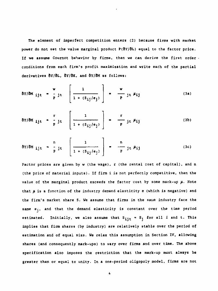
The element of imperfect competition enters (2) because firms with market

power do not set the value marginal product P(8Y/8L) equal to the factor price.

If we assume Cournot behavior by firms, then we can derive the first order

conditions from each firm's profit maximization and write each of the partial

derivatives 8Y18L, WYUK and 8Y/8M as follows:

8Yj8H ijt p jt [ ( e j t Sit (3a)8Y18M -p ;t 1 + (Sij/ej) J (a

r 1 1r8Y/8H4 ijt t [ . (Sij/e ) J] it P ij (3b)

n 1 n

ay/am ijt L I = _it Plj (3c)dy =p jt 1 + (Sij/ej) p

Factor prices are given by w (the wage), r (the rental cost of capital), and n

(the price of material inputs). If firm i is not perfectly competitive, then the

value of the marginal product exceeds the factor cost by some mark-up p. Note

that p is a function of the industry demand elasticity e (which is negative) and

the firm's market share S. We assume that firms in the same industry face the

same ej, and that the demand elasticity is constant over the time period

estimated. Initially, we also assume that Sijt = Sj for all i and t. This

implies that firm shares (by industry) are relatively stable over the period of

estimation and of equal sizs. We relax this assumption in Section IV, allowing

shares (and consequently mark-ups) to vary over firms and over time. The above

specification also imposes the restriction that the mark-up must always be

greater than or equal to unity. In a one-period oligopoly model, firms are not

4

allowed to make short-run losses because such behavior would not be rational.

This restriction is probably unnecessary but is not rejected by the data (see

Section III).

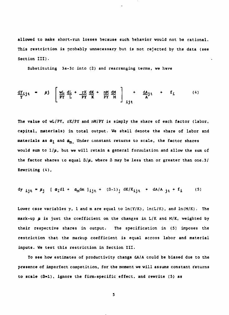
Substituting 3a-3c into (2) and rearranging terms, we have

dYijt #ji wL dL + rK dK + nM dM + dAjt + fi (4)Y PY L PY K PY M A~.Xijt ~ [wLd+ rKdK+ M~ ~ ~ ~i (4

The value of wL/PY, rK/PY and nM/PY is simply the share of each factor (labor,

capital, materials) in total output. We shall denote the share of labor and

materials as a, and am. Under constant returns to scale, the factor shares

would sum to 1/p, but we will retain a general formulation and allow the sum of

the factor shares to equal B/p, where B may be less than or greater than one.3/

Rewriting (4),

dy ijt - /j [ aldl + lmdm ]ijt + (3-l)j dK/Kijt + dA/A jt +fi (5)

Lower case variables y, 1 and m are equal to ln(Y/K), ln(L/K), and ln(M/K). The

mark-up i is just the coefficient on the changes in L/K and M/K, weighted by

their respective shares in output. The specification in (5) imposes the

restriction that the markup coefficient is equal across labor and material

inputs. We test this restriction in Section III.

To see how estimates of productivity change dA/A could be biased due to the

presence of imperfect competition, for the moment we will assume constant returns

to scale (B-1), ignore the firm-specific effect, and rewrite (5) as

5

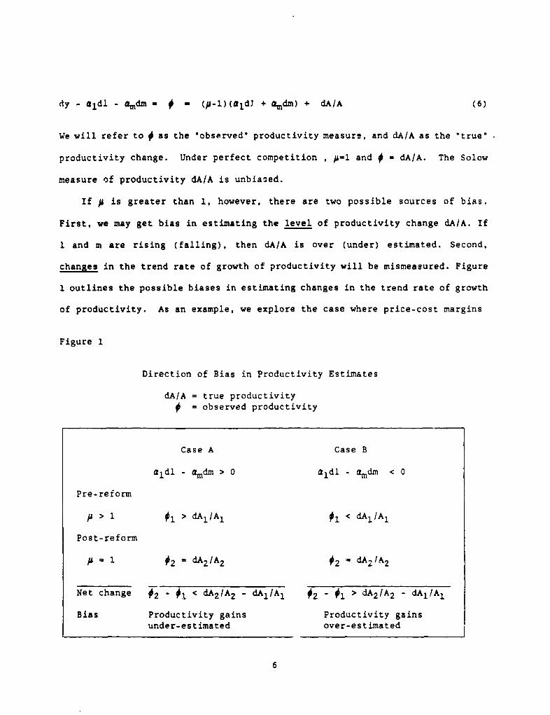
dy - ldl- - adm - (p-l)(a1d1 + lmdm) + dA/A (6)

We will refer to # as the "observed' productivity measure, and dA/A as the 'true"

productivity change. Under perfect competition , p=l and * - dA/A. The Solow

measure of productivity dA/A is unbiased.

If # is greater than 1, however, there are two possible sources of bias.

First, we may get bias in estimating the level of productivity change dA/A. If

1 and m are rising (falling), then dA/A is over (under) estimated. Second,

changes in the trend rate of growth of productivity will be mismeasured. Figure

1 outlines the possible biases in estimating changes in the trend rate of growth

of productivity. As an example, we explore the case where price-cost margins

Figure 1

Direction of Bias in Productivity Estimates

dA/A = true productivity= observed productivity

Case A Case B

aidl - amdm > O a1dl - amdm < 0

Pre-reform

# > 1 Oi > dAj/A 1 1 < dAj/Al

Post-reform

= 1 02 = dA2/A2 = dA,/A2

Net change 02 - 01 < dA2/A2 - dAl/Al 02 - 01 > dA2/A2 - dAl/A1

Bias Productivity gains Productivity gainsunder-estimated over-estimated

6

exceed one and firms have market power prior to a trade reform. In this case,

the level of observed productivity 0 will be greater (1gss) than the true measure

if 1 and m are rising (falling). If the trade reform is accompanied by a fall

in market power (possibly due to increases in the perceived elasticity of

demand), price-cost margins fall to unity and measured productivity will equal

the true productivity measure dA/A. However, if we are interested in comparing

productivity before and after the changes in trade policy, we are likely to

incorrectly assess the true change in dA/A. As illustrated in Figure 1, the

direction of the bias cannot be predicted on the basis of (6)t we ars equally

likely to overestimate or underestimate the increase in productivity following

the reform.

To see how estimates oi productivity dA/A could be biased due to increasing

or decreasing returns to scale, let us assume perfect competition (it - 1) and

rewrite (5) as (6)'

dy - aldl - amdm - 0 - (3-1)j dK/K + dA/A (6)'

If 3 exceeds 1, then the technology is characterized by increasing returns.

Observed productivity measure will exceed the true value dA/A as long as dK/K

is positive, so TFP is over-estimated. Under decreasing returns, TFP will be

under-estizrated. Since increasing returns are consistent with imperfect

competition, empirically we should observe b greater than 1 and market power

concurrently.

7

II. Trade Policy in the Cote d'Ivoire

The trade regime in the Cote d'Lvoire becamp increasingly restrictive in the

1970a. In 1973. a major restructuring of the tariff code increased nominp1 tariff

rates and raised levels of effective protection by implementing an escalated

tariff structure. In the second half of the 1970s and in the early 1.980s,

quantitative restrictions and arbitrary reference prices were introduced on a

wide range of imports competing with domestic manufactures. Table ; indicates

the extent of trade protection across industrial sectors before the reform, as

measured by effective protection coefficicnts and the number of import licences

(quotas) issued across sectors. Textiles and food-related manufacturing received

the highest effective protection, followed by chemicals. Quotas were also high

in food processing and beverages, followed by textiles and chemicals.

During the boom years in the second half of the 1970s, the Cote d'Ivoire

benefitted from the surge in world coffee and cocoa prices. The increases in

revenue, most of which were captured by the government, were used to promote

investment and expand public spending and infrastructure. The severe

macroecononic imbalances that followed the fall in coffee prices forced the

government to adopt an austerity program in 1982. The adjustment program was

followed by a major trade reform introduced in mid-1984.

The trade reform was implemented in 1985 ar 4xtended in 1986 and early 1987.

The reform removed quantitative restrictions and reference prices, rationalized

the tariff structure, and introduced temporary tariff surcharges. The goal of

the tariff reform was to equalize effective protection across different sectors

by lowering tariffs on final goods and raising tariffs on inputs and intermediate

goods. The surcharges declined over a five-year period to allow firms previously

protected by non-tariff measures to adjust. Tariff changes and the removal of

8

quotas was implemented in two phases. In the first phase (1985), reforms were

imposed on key sectors including textiles and food processing, In the second

phase (late 1986, early 1987), the reform was extended to the rest of the

manufacturing sector (fertilizers, machinery).

Cote d'Ivoire's nominal exchange rate is fixed in relation to the French

franc at a rate which ic the same for a number of franc zone African countries.

When the french franc appreciated against the US dollar between 1985 and 1988,

the Ivorian franc became considerably overvalued in real terms. Consequently,

the reform was conducted in conjut.ction with an envircnment which lowered the

competitiveness of exports on world markets. lthough the government simulated

a partial devaluation through an export subsidy scheme for manufactured exports,

the first subsidy payments were delayed until mid-1986 and payments were

concentrated in several large firms. The government's inability to compensate

exporting firms for the real appreciation meant th&t the export sector was

adversely affected. Consequently, we should see a fall in price-cost margins for

exporting sectors in the post trade reform period.

To account for changes in behavior and productivity during the trade

reforms in Cote d'Ivoire, we will want to modify (5) to allow for a change in

mark-ups by firms during the post-1985 period. Changes in behavior would be

captured by adding an interactive slope dummy to dx in (5). If trade reform

induced a shift in the overall level of productivity, then we should also include

an intercept dummy. We then have the estimating equation:

dy ijt = Bljdxijt + B2; (D dx ]ijt + B3j D + B4j dkijt + dA/A jt + fi (7)

where BljB4j w(-)dx * alldl + amdmdk - dK/K

9

D is 1 for 1985-87 and 0 otherwise. If trade policy changes did in fact lead to

more competitive firm Lehavior, the coefficient B2 on (D dx] should be negative,

reflecting the fall in mark-ups when firms are exposed to international

competition. The coefficient B4 is equal to the scale parameter 3 minus one. If

the coefficient is greater than zero, the technology is characterized by

increasing returns; if it is equal to zero, constant returns; if less than zero,

decreasing returns. The productivity term dA/A can be thought of as the sum

of a constant industry level rate Boj plus a residual uit. This yields our final

estimating equation:

dy ijt - Bljdxijt + B2j [D dx )ijt + B3j D + B4j dkijt + Boj + fi + uit (7)

If the individual effect fi is fixed, we can estimate (7) using a standard fixed

effect approach. Tf, however, fi is random, then estimating (7) as a fixed effect

model will yield consistent but inefficient estimates. Under a random effect

model, the most efficient estimate of (7) requires generalized least squares

(GLS). 4/ Since the individual effect in (1) is modelled as a difference in

production technology which is not likely to vary randomly across individuals,

the fixed effect model is probably the more appropriate specification.

Data

The firm data is taken from information sent to the Banque de Donnees

Financieres (BdDF), which is instructed to gather annual information on all

industrial firms. The number of firms in individual years ranges from around

250 in the mid-1970s to nearly 500 in the mid-1980s. Although the coverage of

10

the industrial sector is incomplete (informal enterprises are excluded and small

formal firms are under-represented), the BdDF covers almost all large and medium-

size formal manufacturing enterprises. We chose our sample of 287 firms by

selecting out those enterprises with a complete time series. Although we include

firms which were only present during part of the 1975-1987 period, we exclude

firms which had missing values between their entry and exit dates. Table 2 shows

that our sample includes the major firms in each of the manufacturing subsectors.

The sample firms accounted for over half of all sales in 1987 for all sectors

covered. For 10 of the 13 sectors, these firms accounted for over 70 percent of

all output in 1987.

We estimate (7) using our panel of 287 Ivorian firms during the period 1975

to 1987. Since firms in different sectors are likely to exhibit different

degrees of competition and face different sets of demand elasticities, we

estimate the equation separately across 9 sectors (see Table 2). The approach

requires data on real output, capital stock, labor and material inputs, and the

shares of labor and materials in total output. Total sales and material inputs

were deflated by 2 digit sectoral level price deflators to obtain a real output

and materials series. We also calculated a material input price deflator based

on input-output tables for each of the sectors, but the estimation results were

unaffected and are not reported here. Real capital stock was constructed in two

steps. First, for those firms that reported across the entire sample period, we

used the perpetual inventory method. Real capital stock in period t is defined

as:

Kit = (l-d)Ki,t_l + It (8)

11

As a benchmark, we used 1976 capital stock for each firm and then added real

investment while accounting for depreciation. Real investment was computed by

deflating nominal investment by sector-specific investment price deflators. To

construct a base year real capital stock for the remaining sample of firms which

entered after 1976, we first constructed a capital stock price deflator (KPD)

using data on firms that were present in all years:

n1 Kijt

KPDjt i-l (9)nv NKijti-i

KPDjt is the capital stock deflator for sector j in year t. It was constructed

using the ratio of the real capital stock computed in (8) to the nominal capital

stock (NK) reported firms that were present in all years. The real base year

capital stock for a firm entering in yeer t is then given by the product

Kijt - (KPDjt) (NKit) (10)

where t is the base year capital stock for firm i. For subsequent years, real

capital stock is then computed using equation (8).

The total number of employees for each firm was used as a measure of labor

input. The dataset does not include hours worked, which is the variable used by

Hall (1988) and Domowitz, Hubbard and Petersen (1988) to measure labor input.

However, using numbers of employees rather than hours should be accurate as long

as there has not been a trend in economy-wide hours per employee. The results

of household surveys for the Cote d'Ivoire (the LSMS World Bank project) for 1985

and 1986 indicate that average hours worked per employee did not change

12

significantly over this two year period. 5/ Since these two years include both

a year of unusual growth (1985) as well as a recession (1986), the fact that

hours worked per employee was relatively stable suggests that the biases in using

numbers of employees should not be too important. However, we cannot dismiss the

possibility that there may have been a trend-line change in hours over the longer

1976-87 period.

Since there are only several firms in some of the industries listed in

Table 2, we aggregated our firm sample into nine sectors: grain processing, food

processing, other food, textiles, chemicals, transport, machinery, wood, and

paper products. Sample means by sector for the pre- and post- trade reform

periods are given in Table 3. Growth rates dropped in 6 of the 9 sectors, but

the average annual growth rate stayed constant, averaging 4.8 percent. Over the

1976-1984 period, the average growth rate is high due to the boom in the economy

in the 1970s. When trade reforms were introduced in 1985, the economy experienced

a period of growth, but 1986 and particularly 1987 was a recessionary period.

The burden of the adjustment appears to have fallen disproportionately on the

labor force, with the annual average growth of employees falling from 2.0

percent to 1.4 percent. One shortcoming of the labor input variable is that it

measures the number of permanent employees hired by the firm, but does not

include information on temporary workers. One possibility, which we do not

investigate, is that the fall in number of permanent employees was accompanied

by an increase in the temporary labor force. However, the fall in employment by

the formal sector, documented in Table 2, has been confirmed by other

studies. 6/

In Table 3, we also report total factor productivity, unadjusted for market

power effects. The productivity measure was calculated using a Tornquist index

13

number formula (see definition in Table 3). Under trade reform, the unadjusted

measure shows productivity increases in most sectors (food processing, chemicals,

transport, machinery, and paper products) but declines in others (textiles and

wood products). On average productivity growth accelerated under the trade

reform, rising from 0.7 percent to 1.5 percent.

III. Estimation

We first estimate (7) using ordinary least squares (OLS) and adopting the

assumption of constant returns to scale. We also estimate (7) assuming

alternately a fixed effect and a random effect specification. Since inputs and

output are jointly determined, however, we then estimate (7) using an

instrumental variables technique. In Section IV we will explore the consequences

of relaxing the assumptions of constant returns and equal mark-ups across firms.

The OLS results, without accounting for fixed effects, are presented in Table

4. The coefficient B1 should measure the extent of market power across sectors,

while B2 indicates the change in price-cost margins under trade reform. The mark-

up of price over marginal cost is highest in the food and textiles sectors,

ranging from 28 percent for the "other food" category to 13 percent for textiles.

We note that these are the sectors with the highest levels of protection prior

to trade reform (refer to Table 1). At the same time, these are also the sectors

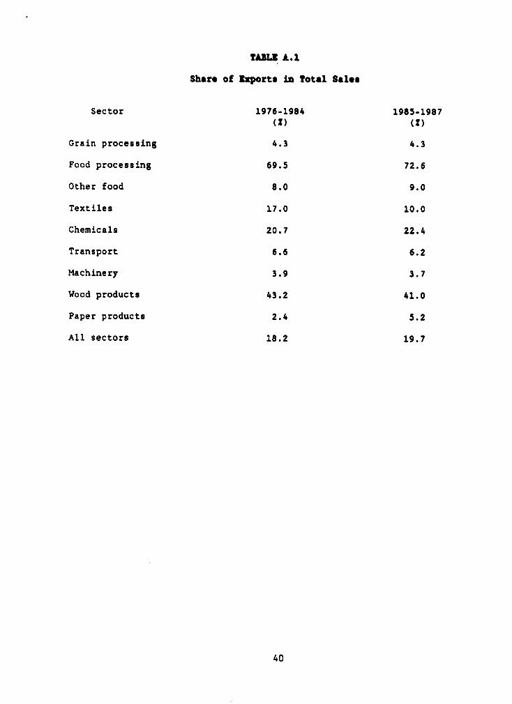
with the greatest degree of outward orientation (See Table A.1). Since we cannot

separate production for export and the domestic market due to the fact that

inputs are not recorded separately, it is impossible to test the hypothesis that

exporters charge high prices in the domestic market but price more competitively

abroad.

14

The coefficient on B2 is negative in six out of nine sectors, which would

support the hypothesis that price-cost margins fell during the trade reforms.

However, B2 is only statistically significant (and negative) for the textile

sector, which suggests that the changes in trade policy generally did not affect

price-cost margins except in the textile sector, where the coefficient has the

expected negative sign. Anecdotal evidence suggests that the conversion of quotas

to tariffs led to large scale underinvoicing, which was particularly severe in

the textile 3ector. For the other sectors, it is possible that changes made in

1987 in the structure of protection for chemicals and transport were too recent

to show up in our data. The coefficient on B3 indicates the change in

productivity growth during the trade policy reforms. The coefficient is positive

for 6 of the 9 sectors, but only statistically significant and positive for the

paper sector. Paper products experienced an unusual increase in growth during

the trade reform period (see Table 3). Since productivity is typically

procyclical, the statistically sig-Lificant increase in productivity growth during

the reform period may only partly be attributed to changes in the trade regime.

We noted earlier that our specification imposes the restriction that mark-

ups are equal across labor and material inputs. We test this restriction by

allowing separate coefficients on labor and material inputs in (5). The F-value

for the null hypothesis that the coefficients are equal is also included in Table

4. Equality of input coefficients is accepted for six out of nine sectors in our

sample. Abbott, Griliches, and Hausman (1989) estimated a similar equation using

US data for the cement industry and found that the restriction of equal

coefficients was not accepted. Rotemberg and Summers (1988) suggest that failure

of the model specification may reflect labor hoarding. We noted earlier that

movements in labor inputs may not be fully reflected due to the possibility of

15

hiring temporary workers. In our data, rejection of the specification test

occurred when the coefficient on the labor input was close to zero, indicating

no correlation between output and labo- inputs. However, the coefficient should

still capture price-cost margins because of movements in material inputs.

The specification above ignores any fixed effects which may be specific to

the individual firms. If fixed effects are present, then our estimating equation

is mis-specified and the coefficients may be biased. One way to test for this

possibility is to compare the OLS results with estimates which allow for a firm-

specific effect which is constant over time. We test for this alternative

specification using a standard fixed-effect, within-group estimator. The within

estimates are reported in Table 5. There is virtually no movement in the

parameters. An F-test of the restriction that the OLS and fixed effect

coefficients are equal is accepted for all sectors. Either a fixed effect is not

present, or is removed by estimating the equation in growth rates instead of in

levels. We also explore the possibility that the firm-specific effect fi is

random. If fi is random and not fixed, then estimating a fixed effect model using

OLS will be unbiased but not as efficient as generalized least squares estimation

(GLS). The GLS estimates are presented in Appendix Table A.2. The random effects

specification does not yield statistically differEnt estimates from OLS.

The OLS estimates are likely to be biased since inputs and output are

simultaneously determined by the firm. Table 6 presents instrumental variables

(IV) estimates under the maintained assumption of constant returns to scale. The

instruments should be correlated with the endogenous right-hand side variables

dX and D dX but independent of any demand or productivity shocks. As instruments

we use the second lag of the nominal exchange rate, a price index for energy,

the second lags of employment and materials, and the second lag of the firm's

16

debt to sales ratio. The price of energy should be correlated with input

decisions but independent of any demand shocks or productivity shocks affecting

the firm. We use the second lag (in levels) for inputs instead of the first lag

since the right-hand side variables already include current and lagged values.

We also include the second lag of the firm's debt to sales ratio, under the

assumption that the firm's borrowings should be correlated with ability to expand

inputs but are predetermined.

Following Bowden and Turkington (1984), we instrument the product D dX using

a nonlinear combination of the dummy D and dX. In our case, this is just the set

of variables D, instruments for dX, and the product of D and the instruments.7/

The instrumental variable estimates in Table 6 were tested for stability using

various alternative sets of instruments, including a composite wage index. Our

experience (which is confirmed by Abbot et al (1989)) suggests that the standard

instruments which are used in these types of regressions, such as GNP, are likely

to be correlated with the error term and may lead to biased estimates of price-

cost margins. Alternative specifications which employed GNP as an instrument

in the first stage of the regression led to rejection of the over-identification

tests for the exogeneity of our instruments. 8/

The estimated coefficients in Table 6 show a similar pattern to the OLS

estimates. Mark-ups are highest for food-related and textile firms. However,

due to the larger standard errors, we can only reject the null hypothesis of

perfect competition for one of the food sectors, machinery, and wood products.

Mark-ups generally fall during the trade reform period, ds indicated by the

negative coefficient on B2. The fall in mark-ups is statistically significant

(and negative) for three sectors: food processing, textiles, and wood products.

Since the level of protection in textiles was quite high before the trade reform,

i7

it is likely that the fall in quotas contributed to lower mark-ups. The fall in

margins for food processing and wood products, however, seems to be linked to

the adverse impact of the franc's appreciation. Table A.1 shows the share of

exports in total sales for the firms in our sample. The food processing (cocoa,

coffee) and wood sectors are the most export oriented of all nine sectors.

Despite the subsidies to offset the negative impact of appreciation on exporters,

it appears that the outward oriented sectors were most negatively affected during

the trade reform.

Table 6 reports the F-value when we test the restriction that the price-

cost margin cannot fall below one, which is an implication of our model. For all

sectors, margins were either positive or not statitistically different from

unity. We also test the validity of our instruments in Table 6. Newey (1985)

suggests a chi-square test which may be applied if the estimating equation is

overidentified and a subset of the instruments is assumed to be valid. A

regression of the residuals from the first stage regression on the instruments

yields a chi-square test of the validity of our instruments. The results of this

test, shown in Table 6. suggest that in all cases our instruments are valid.

IV. Alternative Specifications

Increasing or Decreasing Returns to Scale

One important source of mis-specification arises from assuming that the

technology is characterized by constant returns, which permits us to omit dk from

equation (7). Recall from (7) that the coefficient on dk is given by B-1, where

13 is the returns to scale parameter. Under constant returns, B equals 1 and the

18

coefficient on dk is zero. Under increasing returns, however, B exceeds one and

the coefficient on dk is positive. If the technology is not characterized by

constant returns, then omitting dk induces a classic omitted variable bias. The

extent of the bias is given by the product R (B-1), where 13-1 is the coefficient

on dk and R is the coefficient of dk regressed on dx (see Schmidt (1976)).

Assuming that R is negative, price-cost margins will be under-estimated with

increasing returns to scale. If, on the other hand, the technology exhibits

decreasing returns, the margins are over-estimated.

We investigate the possibility of bias due to the technology assumptions

in Table 7. Table 7 shows the same pattern of price-cost margins as earlier

estimates. Margins are highest in textiles, export-related products (wood, food

processing), and chemicals. The coefficient on dk is statistically significant

for one product group, "other food". For this product, the mark-up falls when

the capital stock is included in the regression equation. The negative

coefficient on the capital stock variable, whict' indicates decreasing returns,

means that price-cost margin are over-estimated for that sector. For all other

sectors, however, the coer.icient on the capital stock variable is not

significant. For most of our sample, specification of the technology as

characterized by constant returns is not inappropriate.

Another potential shortcoming of the original specification is the

assumption, implicit in the first order conditions 3a-3c, that the value of the

marginal prod_.ct of capital is set equal to a mark up # multiplied by the cost

of capital (r) in every period. A profit-maximizing firm might choose labor (L)

and materials (M) in the short run, and take capital (K) to be predetermined.

It can be shown that if we alter the original maximization problem of the firm

so that the production technology is given by

19

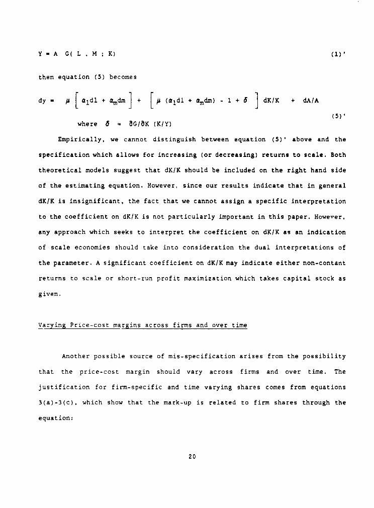
Y - A G( L , M ; K) (1)'

then equation (5) becomes

dy ' [aldl + amdm I + (aidl + amdm) - 1+5 ] dK/K + dA/A

(5)'where 6 = OG/8K (K/Y)

Empirically, we cannot distinguish between equation (5)' above and the

specification which allows for increasing (or decreasing) returns to scale. Both

theoretical models suggest that dK/K should be included on the right hand side

of the estimating equation. However, since our results indicate that in general

dK/K is insignificant, the fact that we cannot assign a specific interpretation

to the coefficient on dK/K is not particularly important in this paper. However,

any approach which seeks to interpret the coefficient on dK/K as an indication

of scale economies should take into consideration the dual interpretations of

the parameter. A significant coefficient on dK/K may indicate either non-contant

returns to scale or short-run profit maximization which takes capital stock as

given.

Varying Price-cost margins across firms and over time

Another possible source of mis-specification arises from the possibility

that the price-cost margin should vary across firms and over time. The

justification for firm-specific and time varying shares comes from equations

3(a)-3(c), which show that the mark-up is related to firm shares through the

equation:

20

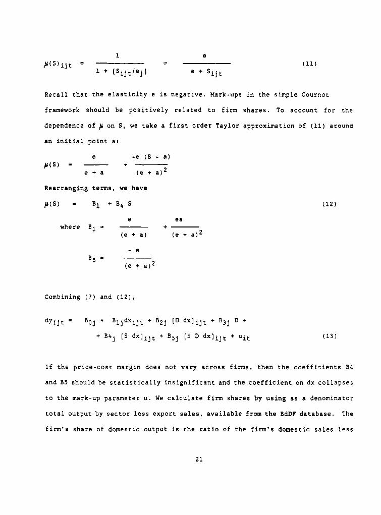
1 ep(S)ijt = (11)

1 + (Si jt/ej] e + Sijt

Recall that the elasticity e is negative. Mark-ups in the simple Cournot

framework should be positively related to firm shares. To account for the

dependence of p on S, we take a first order Taylor approximation of (11) around

an initial point a:

e -e (S - a)/A(S) - +

e + a (e + a)2

Rearranging terms, we have

/5(S) - B1 + B4 S (12)

e eawhere B1 = +2

(e + a) (e + a)2

- e

B5 = (e + a)2

Combining (7) and (12),

dyijt BOj + Blidxijt + B2j (D dx)ijt + B3j D +

+ B4; (S dx]ijt + B5j (S D dx]ijt + uit (13)

If the price-cost margin does not vary across firms, then the coefficients B4

and B5 should be statistically insignificant and the coefficient on dx collapses

to the mark-up parameter u. We calculate firm shares by using as a denominator

total output by sector less export sales, available from the BdDF database. The

firm's share of domestic output is the ratio of the firm's domestic sales less

21

export sales to total sector (domestic) output. One of the shortcomings of this

approach is the lack of import data. Consequently, the variable S does not

represent the firm's share of total domestic consumption, but it does indicate

the firm's share of domestically produced output.

In Table 8, our es imates for (13) show that the coefficient on S is

statistically insignificant across all sectors. The statistical insignificance

of S seems to indicate that differences in shares, either across firms and over

time, are not a source of varying mark-ups. The patterns observed earlier are

also exhibited in Table 8. Price-cost margins are highest for textiles and export

oriented sectors. Nevertheless, there are a number of problems with this

approach. The coefficient on S should be positive (see equation 12), yet for

half the sectors it is in fact negative. One possibility is that a simple Cournot

model may not be appropriate as an explanation for the observed mark-ups. Another

problem is that firm shares are calculated as a fraction of total domestic

output. Finally, the estimates may be highly imprecise since nearly all the

right-hand side variables are endogenous. Nevertheless, our instrumental

variables estimates in Table 8 do give statistically significant coefficients

for the price-cost mark-up, in contrast to the insignificant estimates on S. In

future work, it may be desirable to explore the dependence of the price-cost

margin on other (possibly firm-specific' factors.

Changes in Capacity Utilizaticn

Another possible source of misspecification arises from the fact that

observed price-cost margins may fluctuate as capacity utilization changes over

the business cycle. If, for example, trade reform was accompanied by contractions

22

in output of the tradeable sectors, then changes in mark-ups may reflect capacity

changes rather than shifts in competitive behavior. In this case, we only observe

measured capital stock K . The true K is equal to K E, where E reflects changes

in utilization of capacity.

If the production function is given by Y - A g(L,K*E,M) then the resulting

estimating equation becomes

dy - de - Bo + Bl { aldl + amdm - (a, + am) de}

+ B2 CD { aldl + amdm - (a, + am) de } ] + B3 D (14)

Since we do not have estimates of capacity utilization at the firm level, we

employ a measure of total energy use as a proxy. A plant's energy use is the

input component most likely to vary as capacity utilization fluctuates. The OLS

and instrumental variable estimates for equation (14) are shown on Table 9. The

general patterns observed earlier are reproduced again in Table 9. In addition,

the fall in margins becomes even more significant following the trade reform,

for both the OLS and the instrumental variable estimates.

V. Modified TFP Estimates

In Section I we showed that TFP can be mismeasured in the presence of either

imperfect competition or non-constant returns to scale. The results from Section

III indicate that market power cannot be rejected for a number of manufacturing

sectors in the Cote d'Ivoire. Here we incorporate those findings to analyze

productivity before and after the trade reforms.

Although productivity may be estimated in a number of different ways, one

23

standard approach is to use the Tornquist index number formula, which is a

discrete approximation to the formula derived in equation (6):

TFP - (In Yt - In Yt.1- Cal (ln Lt - ln Lt-i ) + am (ln Mt - ln Mt-,)

+ (1 - al - am )(In Kt - ln Kt-. )] (15)

where al 1/2 (alt + alt_l)

am 5 1/2 (amt + amt-l)

If we incorporate the mark-up factor p, equation (15) can be written as:

TFP - (in Yt ln Yt-_] - # (a, (ln Lt - ln Lt_1 ) + am (ln Mt - ln Mt_,)

+ (1/p - a, - am )(ln Kt - ln Kt_l )] (16)

Estimates of # were taken from Table 9 to calculate revised TFP estimates

before and under the trade reforms. Estimates of productivity using both the

original and revised definitions (equations (15) and (16) respectively) are

presented in Table 10. Since the model imposes the restriction that the price-

cost margin must be greater than or equal to unity, we impose the restriction

that margins cannot fall below unity. The original estimates are reproduced from

Table 3. Under the assumption of perfect competition, we find that productivity

increased under trade reform for six of the nine sectors. Over all sectors,

productivity rose from an average of .7 to 1.5 percent annually. If we relax

the assumption of perfect competition, the gain in productivity is much smaller.

Productivity only rises in 5 sectors, with smaller increases overall. Since

labor and material inputs per unit of capital experienced negative growth prior

to 1985, TFP is underestimated in equation (15), and the change in productivity

after 1985 is overstated. On average, the adjusted productivity measure only

rises slightly, from .7 to .9 percent growth annually. The results in Table 10

24

suggest that productivity estimates are highly sensitive to the assumption of

perfect competition. For example, in the food sector when we introduce imperfect

competition, the gain in productivity post-reform rises from .8 percent to 2-

percent annually. On average, our data suggests that when we incorporate

imperfect competition into the productivity estimates, there is no apparent

relationship between productivity and trade reform. However, two aspects of the

reform must be acknowledged. First, the estimated time period for the sample post

reform is only three years. If there are any productivity gains associated with

trade reform, such gains may only appear over a longer time period. Second, the

reform was accompanied by a real appreciation of the currency, which adversely

affected exporting sectors. Table 10 shows that productivity fell primarily in

exporting sectors, but generally increased in other sectors.

Conclusion

Research on pruductivity has often focused on the relationship between

productivity increases and structural changes in an economy, such as trade policy

reform. If, however, those structural changes affect the nature of competition

or have scale effects, then both the levels and the changes in productivity may

be mismeasured. In this paper, we extend previous studies to measure the

relationship between productivity, market power, and trade reform.

Using a panel of 287 firms in the Cote d'Ivoire, we test for imperfect

competition before and after the 1985 trade reform. We find that protected

sectors such as textiles have significant mark-ups of price over marginal cost.

We also find evidence that price-cost margins fell between 1985 and 1987.

However, the fall in mark-ups for exporting sectors is likely to be linked more

25

to the real appreciation of the currency than to increases in domestic

competition.

If we incorporate measures of price-cost margins into estimates of

productivity, we find that these estimates are extremely sensitive to the usual

assumptions made about competition. Whereas there seems to be a strong

relationship between trade reform and productivity when we assume perfect

competition in the product markets, this relationship almost disappears when we

allow for varying mark-ups. These results may be qualified, however, by noting

that when the exporting sectors are excluded from the analysis, there are

productivity gains associated with trade reform. The results support recent

arguments (see Rodrik (1988)) that the theoretical basis for a positive link

between trade reform and productivity growth should be explored in future

research. More analytical efforts are needed which explicitly model the possible

links between trade policy and productivity growth.

26

Notes

1/ For an overview of this literature, see Helpman and Krugman (1989).

2/ An exception is de Melo and Urata (1986), which compares reported price-costmargins for two census years before and after reforms in Chile. Research ondeveloped country data includes Domowitz, Hubbard, and Petersen (1986), who useaggregate data to find a negative relationship between import penetration andreported price-cost margins.

3/ To see why this holds, say we have a production function given byY = ALaMbKc, where a + b + c sum to 3, the scale parameter. If wetake logs and differentiate, we see that

dY L dY M dY K- = a + b + c - B

dL Y dM Y dK Y

dY LBut from our first order conditions, -- - = Y a1 , etc. so

dL Y

we have j al + p am + I ak = '-

4/ For a description of GLS for panel data, see Hsiao (1986).

5/ A regression of hours worked on several control variables (sex, age, location,education) and a year dummy yielded an insignificant coefficient on the yeardummy with a t-statistic of 1.54.

6/ See 'Cote d'Ivoire: Industrial Competitiveness During Economic Crisis ardAdjustment", Klaus Lorch, 1989.

7/ If instead we had regressed dx on a set of instruments to obtain a predictedvalue for dx, and then calculated the predicted dx multiplied by Dl, this wouldhave yielded a biased coefficient on the product dx Dl.

8/ Estimates of the alternative specifications available from the author onre.huest.

27

Bibliography

Abbott, T.A., Z. Griliches and J.A. Hausman, 'Short Run Movements inProductivity: Market Power versus Capacity Utilizatior., mimeo, 1989.

Bhagwati, Jagdish, 'Export-Promoting Trade Strategy: Issues and Evidence",The World Bank Research Observer, January 1988.

Bowden, Roger and Darrell Turkington, Instrumental Variables, CambridgeUniversity Press, 1984.

Domowitz. Ian, R. Glenn Hubbard, and Bruce C. Petersen, 'MarketStructure and Cyclical Fluctuations in U.S. Manufacturing", The Reviewof Economics and Statistics, 1988

------------, 'Business Cycles and the Relationship between concentration andprice-cost margins', Rand Journal of Econcmics, Spring 1986.

Hall, Robert E. 'The Relation between Price and Marginal Cost in U.S.Industry", Journal of Political Economy, October 1988.

Havrylyshyn, Oli, 'Trade Policies and Economic Efficiency in DevelopingCountries: A Literature Survey', 1987, World Bank.

Helpman, Elhanan and Paul Krugman, Trade Policy and Market Structure, MIT Press,1989.

Hsiao, Cheng, Analysis o: Fanel Data, Cambridge University Press, 1986.

Lorch., Klaus, 'Cote d''voire: Industrial Competitiveness During Economic Crisisand Adjustment', World Bank, 1989.

Newev, W,hitney, 'Generalized Methocl of Moments Specification Testing", Journalof Econometrics, vol 29, 185.

Nishimizu, Mieko, and John M. Page, Jr., 'Economic Policies and ProductivityChange in :ndustry: An :nterr.ational Comparison', World Bank, 1987.

Nishimizu, M`eko and Sherman Robinson, 'Trade Policies and Productivity Changein Semi-Industrialized Countries', Journal of Development Economics, vol. 16,September/October 1984.

Nishimizu, Mieko, 'Cn the Methodology and the Importance of the Measurement ofTotal Factor Productivity Change: the State of the Art', 1979.

Rodrick, Dani, 'Closing the Technology Gap: Does Trade LiberalizationReally Help?', mimeo, Harvard University, 1988.

Rotemberg, Julio, and Lawrence Surmers, 'Labor Hoarding. Inflexible Prices andProcyclical Productivity', NBER Working Paper 2591, May 1988.

28

Schmidt, Peter, Econometrics, Mark Dekker, Inc.; 1976.

Solow, Robert M., "Technical Change and the Aggregate Production Function",Review of Economics and Statistics, August 1957.

World Bank, "The Cote d'Ivoire in Transition: From Structural Adjustment toSelf-sustained Growth", 1987.

29

TABLE 1

Estimates of Protection Across Sectors,1980 and 1982

Nominal Tariff Effective Tariff Occurences ofProtection Protection Import Licenses

Sector Coefficient 1980 C fficient 1980 1982

I Food Processingand Beverages

Grain processing - - 6Food processing 1.359 3.340 34Beverages - - 17Oils 1.405 1.829 2Other 1.493 1.829 0

II Textiles

Clothing 1.422 2.455 182Leather, footwear 1.303 1.307 39

III Chemicals

Chemicals 1.309 1.337 52Rubber 1.387 1.489 10

IV Transport, Machinery

Transport 1.245 1.245 17Machinery 1.230 1.230 9

V Wood, paper products

Wood 1.258 1.276 4Paper

Source: 'The C6te d'Ivoire in Transition: From Structural Adjustment to Self-sustained Growth," World Bank, 1987

30

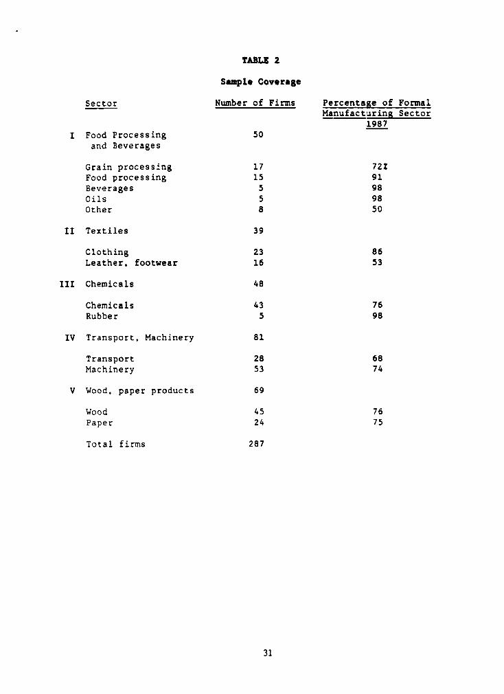
TABLE 2

Sample Coverage

Sector Number of Firms Percentage of FormalManufacturing Sector

1987

I Food Processing 50and Beverages

Grain processing 17 72ZFood processing 15 91Beverages 5 98Oils 5 98Other 8 50

II Textiles 39

Clothing 23 86Leather, footwear 16 53

III Chemicals 48

Chemicals 43 76Rubber 5 98

IV Transport, Machinery 81

Transport 28 68Machinery 53 74

V Wood, paper products 69

Wood 45 76Paper 24 75

Total firms 287

31

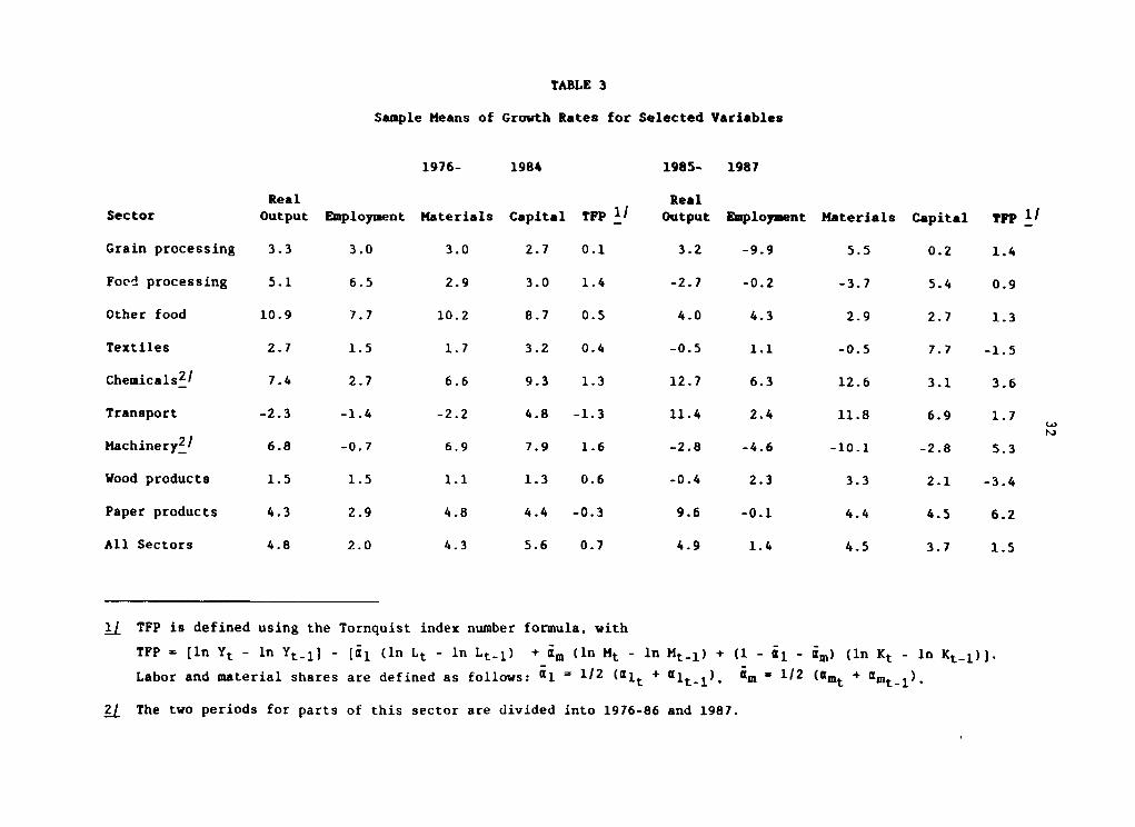
TABLE 3

Sample Heans of Growth Rates for Selected Variables

1976- 1984 1985- 1987

Real Real

Sector Output Employment Materials Capital TFP 1/ Output Employment Materials Capital tFP

Grain processing 3.3 3.0 3.0 2.7 0.1 3.2 -9.9 5.5 0.2 1.4

Foed processing 5.1 6.5 2.9 3.0 1.4 -2.7 -0.2 -3.7 5.4 0.9

Other food 10.9 7.7 10.2 8.7 0.5 4.0 4.3 2.9 2.7 1.3

Textiles 2.7 1.5 1.7 3.2 0.4 -0.5 1.1 -0.5 7.7 -1.5

Chemicals 2 ' 7.4 2.7 6.6 9.3 1.3 12.7 6.3 12.6 3.1 3.6

Transport -2.3 -1.4 -2.2 4.8 -1.3 11.4 2.4 11.8 6.9 1.7

Machinery 2 / 6.8 -0.7 6.9 7.9 1.6 -2.8 -4.6 -10.1 -2.8 5.3

Wood products 1.5 1.5 1.1 1.3 0.6 -0.4 2.3 3.3 2.1 -3.4

Paper products 4.3 2.9 4.8 4.4 -0.3 9.6 -0.1 4.4 4.5 6.2

All Sectors 4.8 2.0 4.3 5.6 0.7 4.9 1.4 4.5 3.7 1.5

I/ TFP is defined using the Tornquist index number formula, with

TFP = [ln Yt - ln Yt-1] [al (ln Lt - ln Lt-1) + im (ln Mt - ln Mt-1) + (1 - 1 - am) (ln Kt - ln Kt-l)J.

Labor and material shares are defined as follows: Ml = 1/2 (alt + CIt_I), am - 1/2 (amt + amt_l).

2/ The two periods for parts of this sector are divided into 1976-86 and 1987.

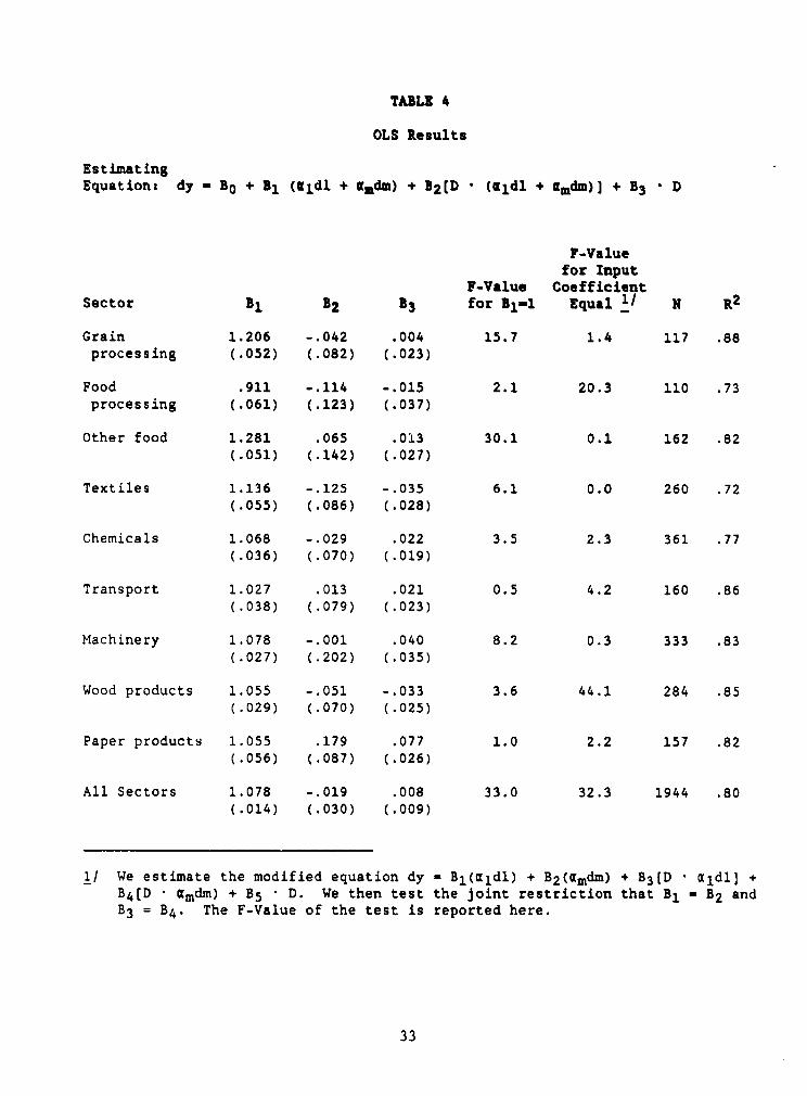
TABLE 4

OLS Results

EstimatingEquation: dy - Bo + Bl (1ldl + ffdm) + B2(D (ildl + amdm)J + B3 D

F-Valuefor Input

F-Value CoefficientSector Bl B2 B3 for Bl-1 Equal 1/ N R2

Grain 1.206 -.042 .004 15.7 1.4 117 .88processing (.052) (.082) (.023)

Food .911 -.114 -.015 2.1 20.3 110 .73processing (.061) (.123) (.037)

Other food 1.281 .065 .013 30.1 0.1 162 .82(.051) (.142) (.027)

Textiles 1.136 -.125 -.035 6.1 0.0 260 .72(.055) (.086) (.028)

Chemicals 1.068 -.029 .022 3.5 2.3 361 .77(.036) (.070) (.019)

Transport 1.027 .013 .021 0.5 4.2 160 .86(.038) (.079) (.023)

Machinery 1.078 -.001 .040 8.2 0.3 333 .83(.027) (.202) (.035)

Wood products 1.055 -.051 -.033 3.6 44.1 284 .85(.029) (.070) (.025)

Paper products 1.055 .179 .077 1.0 2.2 157 .82(.056) (.087) (.026)

All Sectors 1.078 -.019 .008 33.0 32.3 1944 .80(.014) (.030) (.009)

1/ We estimate the modified equation dy Bl(aldl) + B2(gmdm) + B3 [D * aldl] +B4[D * aMdm) + B5 * D. We then test the joint restriction that B1 = B2 andB3 = B4. The F-Value of the test is reported here.

33

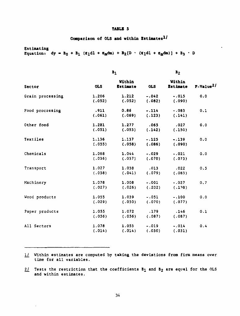
TABLE 5

Comparison of OLS and vithin Eutiuateal/

EstimatingEquation: dy - Bo + Bl (Eldl + £mdm) + B2 [D , (1ldl + amdm)J + B3 D

B1 B2

Vithin VithinSector OLS Estimate OLS Estimate F-Value2'

Grain processing 1.206 1.212 -.042 -.015 0.0(.052) (.052) (.082) (.090)

Food processing .911 0.86 -.114 -.083 0.1(.061) (.069) (.123) (.141)

Other food 1.281 1.277 .065 .027 0.0(.051) (.053) (.142) (.150)

Textiles 1.136 1.137 -.125 -.139 0.0(.055) (.058) (.086) (.090)

Chemicals 1.068 1.044 -.029 -.021 0.0(.036) (.037) (.070) (.073)

Transport 1.027 1.038 .013 .022 0.5(.038) (.041) (.079) (.083)

Machinery 1.078 1.008 -.001 -.027 0.7(.027) (.026) (.202) (.118)

Wood products 1.055 1.039 -.051 -.100 0.0(.029) (.030) (.070) (.077)

Paper produicts 1.055 1.072 .179 .146 0.1(.056) (.056) (.087) (.087)

All Sectors 1.078 1.053 -.019 -.014 0.4(.014) (.014) (.030) (.031)

1/ Within estimates are computed by taking the deviations from firm means overtime for all variables.

2/ Tests the restriction that the coefficients B1 and B2 are equal for the OLSand within estimates.

34

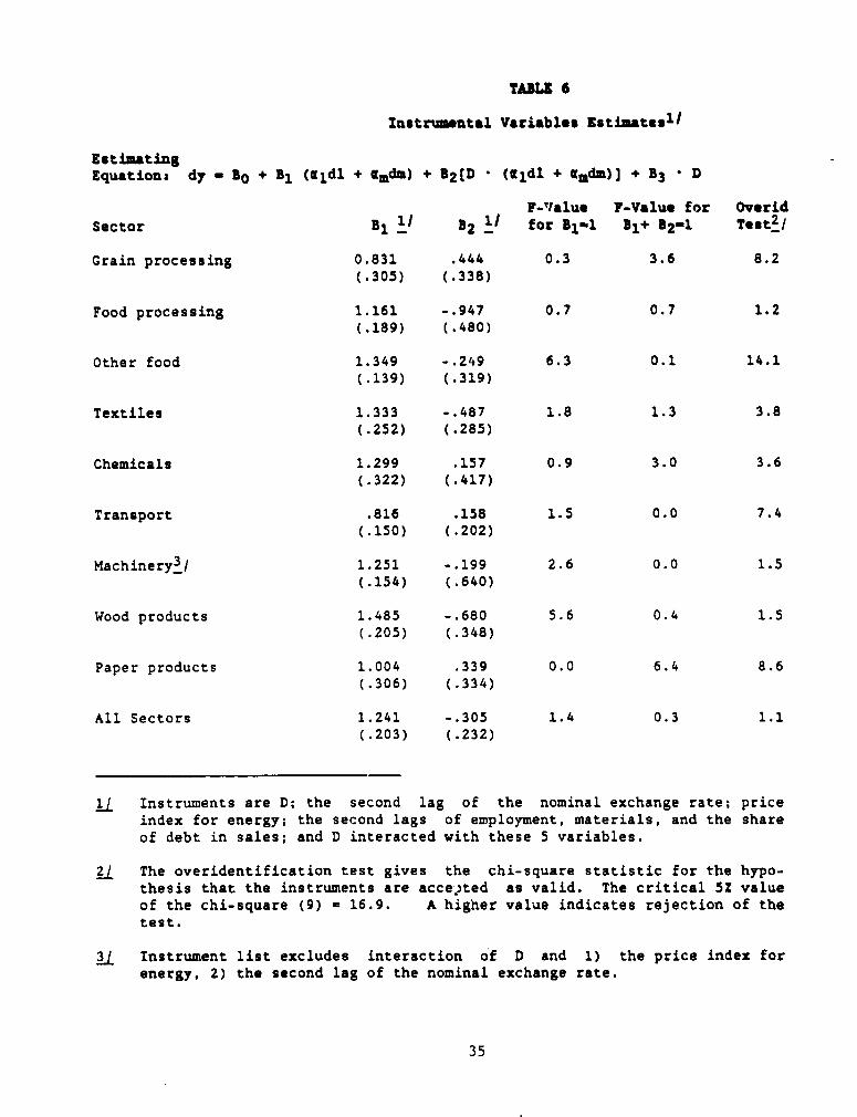
TABLE 6

Instrumntal Variables Estimatesll

Est matingEquation: dy - Bo + B1 (aldl + Lmd3) + B2(D (tldl + RMdm)) + B3 I D

F-'ralue F-Value for Overid

Sector Bi 'l B2 1/ for Bl-l Bi+ B2-1 Test2 I

Grain processing 0.831 .444 0.3 3.6 8.2(.305) (.338)

Food processing 1.161 -.947 0.7 0.7 1.2(.189) (.480)

Other food 1.349 -.249 6.3 0.1 14.1(.139) (.319)

Textiles 1.333 -.487 1.8 1.3 3.8(.252) (.285)

Chemicals 1.299 .157 0.9 3.0 3.6(.322) (.417)

Transport .816 .158 1.5 0.0 7.4(.150) (.202)

Machinery3/ 1.251 -.199 2.6 0.0 1.5(.154) (.640)

Wood products 1.485 -.680 5.6 0.4 1.5(.205) (.348)

Paper products 1.004 .339 0.0 6.4 8.6(.306) (.334)

All Sectors 1.241 -.305 1.4 0.3 1.1(.203) (.232)

1/ Instruments are D; the second lag of the nominal exchange rate; priceindex for energy; the second lags of employment, materials, and the shareof debt in sales; and D interacted with these 5 variables.

2/ The overidentification test gives the chi-square statistic for the hypo-thesis that the instruments are acce?ted as valid. The critical 5Z valueof the chi-square (9) - 16.9. A higher value indicates rejection of thetest.

3/ Instrument list excludes interaction of D and 1) the price index forenergy, 2) the second lag of the nominal exchange rate.

35

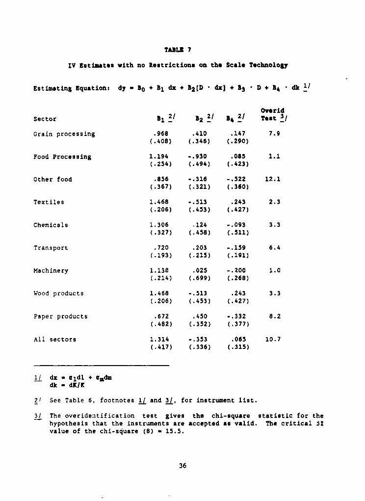
TABLE 7

IV Estimates with no Restrictions on the Scale Technology

Estimating Equations dy- Bo + B1 d + B2(D d xz] + 13 D + B d k.1d

OveridSector Bl 2/ B2 2/ B4 2/ Teat 3/

Grain processing .968 .410 .147 7.9(.408) (.346) (.290)

Food Processing 1.194 -.930 .085 1.1(.254) (.494) (.423)

Other food .856 -.316 -.522 12.1(.367) (.321) (.360)

Textiles 1.468 -.513 .243 2.3(.206) (.453) (.427)

Chemicals 1.306 .124 -.093 3.3(.327) (.458) (.511)

Transport .720 .203 -.159 6.4(.193) (.215) (.191)

Machinery 1.138 .025 -.200 1.0(.214) (.699) (.268)

Wood products 1.468 -.513 .243 3.3(.206) (.453) (.427)

Paper products .672 .450 -.332 8.2(.482) (.352) (.377)

All sectors 1.314 -.353 .065 10.7(.417) (.336) (.315)

1/ dx - ldl + £mdmdk - dK/K

21 See Table 6, footnotes 1/ and 3/, for instrument list.

3/ The overidentification test gives the chi-square statistic for thehypothesis that the instruments are accepted as valid. The critical 52value of the chi-square (8) a 15.5.

36

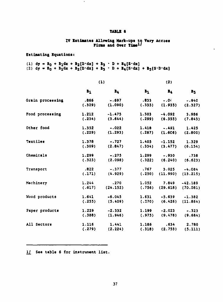
TABUE 6

IV Eatimtes Allowing Mark-ups to Vary AcrossFimrs and Over Timle1

Estimating Equations:

(1) dy - Bo + BldZ + B2(D-dz3 + 5 * D + 34 [Sdx](2) dy - Bo + Bld4 + B2[D-ds] + BS D + 34 [S-dzJ + 35[S-DdzJ

(1) (2)

|1 34 81 34 B5

Grain processing .866 -.697 .833 -.Oi -.940(.329) (1.090) (.335) (1.935) (2.327)

Food processing 1.212 -1.475 1.303 -4.092 3.986(.234) (3.644) (.299) (6.355) (7.843)

Other food 1.352 -.022 1.418 -.491 1.425(.229) (1.293) (.267) (1.6C6) (2.800)

Textiles 1.378 -.727 1.405 -1.152 1.329(.309) (2.847) (.334) (3.477) (6.154)

Chemicals 1.299 -.275 1.299 -.930 .738(.323) (2.098) (.322) (6.240) (6.623)

Transport .822 -.377 .767 3.025 -4.084(.171) (4.929) (.250) (11.990) (13.215)

Machinery 1.244 .270 1.052 7.849 -42.189(.617) (24.152) (.756) (29.618) (70.081)

Wood products 1.641 -6.045 1.631 -5.639 -1.382(.255) (5.409) (.270) (6.426) (11.864)

Paper products 1.229 -2.332 1.199 -2.023 -.323(.388) (1.946) (.975) (9.478) (9.684)

All Sectors 1.116 1.441 1.186 .634 2.780(.279) (2.224) (.318) (2.753) (5.111)

1/ See table 6 for instrument list.

37

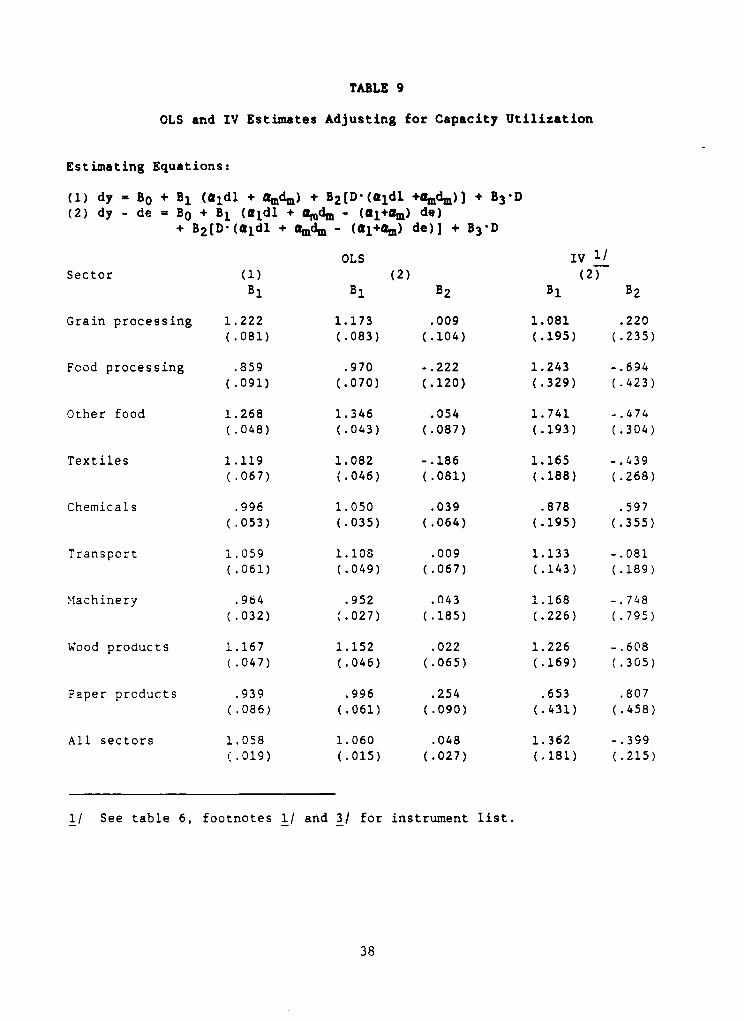
TABLE 9

OLS and IV Estimates Adjusting for Capacity Utilization

Estimating Equations:

(1) dy - Bo + B1 ( 1dl + amdM) + B2(D'(aldl +QmdM)] + B3'D(2) dy - de = Bo + B1 (Qldl + amdm (al+am) de)

+ B2 [Di(aldl + Qmdm (l+Qm) de)] + B3 'D

OLS IVSector (1) (2) (2)

B1 B1 B2 B1 B2

Grain processing 1.222 1.173 .009 1.081 .220(.081) (.083) (.104) (.195) (.235)

Fcod processing .859 .970 -.222 1.243 -.694(.091) (.070) (.120) (.329) (.423)

Other food 1.268 1.346 .054 1.741 -.474(.048) (.043) (.087) (.193) (.304)

Textiles 1.119 1.082 -.186 1.165 -.439(.067) (.046) (.081) (.188) (.268)

Chemicals .996 1.050 .039 .878 .597(.053) (.035) (.064) (.195) (.355)

Transport 1.059 1.108 .009 1.133 -.081(.061) (.049) (.067) (.143) (.189)

Machinery .964 .952 .043 1.168 -.748(.032) %.027) (.185) (.226) (.795)

Wood products 1.167 1.152 .022 1.226 -.608(.047) (.046) (.065) (.169) (.305)

Paper products .939 .996 .254 .653 .807(.086) (.061) (.090) (.431) (.458)

All sectors 1.058 1.060 .048 1.362 -.399(.019) (.015) (.027) (.181) (.215)

1/ See table 6, footnotes 1/ and 3/ for instrument list.

38

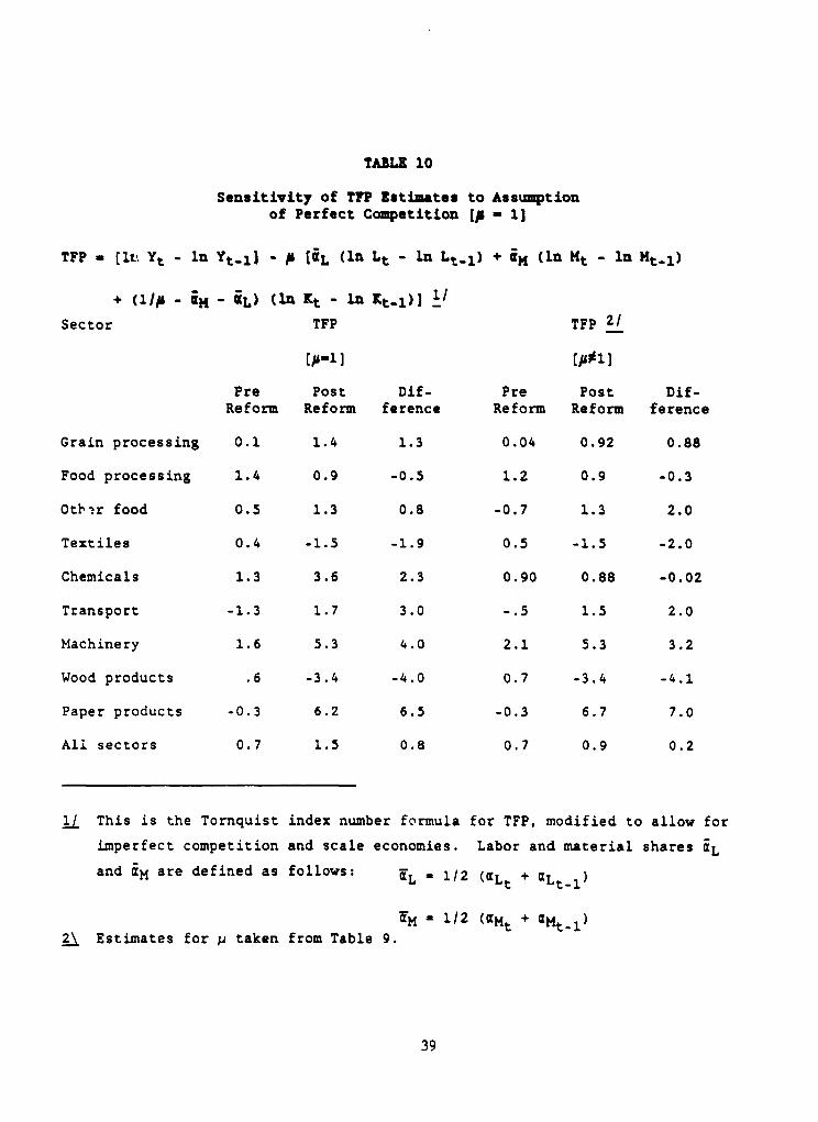
TABLE 10

Sensitivity of TIP Estimates to Assumptionof Perfect Competition lp - 1]

TFP - [112 Yt - ln Yt-1J - is AL (ln Lt - ln Lt-1) + 1M (ln Mt - ln Mt-1)

+ (110 - iM k Z) (la Kt - ln Kt_l)]

Sector TFP TFP 2/

(p-1] (Psi)

Pre Post Dif- Pre Post Dif-Reform Reform ference Reform Reform ference

Grain processing 0.1 1.4 1.3 0.04 0.92 0.88

Food processing 1.4 0.9 -0.5 1.2 0.9 -0.3

Otbir food 0.5 1.3 0.8 -0.7 1.3 2.0

Textiles 0.4 -1.5 -1.9 0.5 -1.5 -2.0

Chemicals 1.3 3.6 2.3 0.90 0.88 -0.02

Transport -1.3 1.7 3.0 -.5 1.5 2.0

Machinery 1.6 5.3 4.0 2.1 5.3 3.2

Wood products .6 -3.4 -4.0 0.7 -3.4 -4.1

Paper products -0.3 6.2 6.5 -0.3 6.7 7.0

All sectors 0.7 1.5 0.8 0.7 0.9 0.2

lj This is the Tornquist index number formula for TFP, modified to allow for

imperfect competition and scale economies. Labor and material shares aL

and aM are defined as follows: aL - 1/2 (MLt + aLt-1)

aM - 1/2 (aMt + aMt_,)

2\ Estimates for y taken from Table 9.

39

TABU A.lI

Share of Ezports in Total Sales

Sector 1976-1984 1985-1987(Z) (Z)

Grain processing 4.3 4.3

Food processing 69.5 72.6

Other food 8.0 9.0

Textiles 17.0 10.0

Chemicals 20.7 22.4

Transport 6.6 6.2

Machinery 3.9 3-7

Wood products 43.2 41.0

Paper products 2.4 5.2

All sectors 18.2 19.7

40

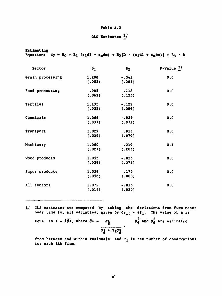
Table A.2

GLS Estimates /

EstimatingEquations dy - Bo + Bl (eldl + mdm) + B2[D (eldl + andm)] + 33 D

Sector Bl B2 F-Value 2/

Grain processing 1.208 -.041 0.0(.052) (.083)

Food processing .905 -.112 0.0(.062) (.125)

Textiles 1.135 -.122 0.0(.055) (.086)

Chemicals 1.066 -.029 0.0(.037) (.071)

Transport 1.029 .013 0.0(.039) (.079)

Machinery 1.060 -.019 0.1(.027) (.203)

Wood products 1.053 -.055 0.0(.029) (.071)

Paper products 1.059 .175 0.0(.056) (.088)

All sectors 1.072 -.016 0.0(.014) (.030)

1/ GLS estimates are computed by taking the deviations from firm meansover time for all variables, given by dyit - ayi. The value of a is

equal to 1 - )7i, where 02 - 2 an 2 or are estimatede n ~aaresitd

V + TiU&

from between and within residuals, and Ti is the number of observationsfor each ith firm.

41

PRE Workng Paper Series

ContactLIWl Author DAIR for paper

WPS429 Ghana's Cocoa Priciig Policy Merrill J. Bateman June 1990 C. SpoonerAlexander Meeraus 30464David M. NewberyWilliam Asenso OkyereGerald T. O'Mara

WPS430 Rural-Urban Growth Linkages in Peter B. Hazell May 1990 C. SpoonerIndia Steven Haggblade 30464

WPS431 Recent Developments in Marketing Panos Varangis May 1990 D. Gustafsonand Pricing Systems for Agricuitural TakamasaAkiyama 33714Export Commodities in Sub-Saharan Elton ThigpenAfrica

WPS432 Policy Choices in the Newly Bela Balassa May 1990 N. CampbellIndustrializing Countries 33769

WPS433 India: Protection Structure and Francois EttoriCompetitiveness of Industry

WPS434 Tax Sensitivity of Foreign Direct Anwar Shah June 1990 A. BhallaInvestment: An Empirical Joel Slemrod 37699Assessm ent

WPS435 Rational Expectations and Boum-Jong Choe June 1990 S. LipscombCommodity Price Forecasts 33718

WPS436 Commodity Price Forecasts and Boum-Jong Choe June 1990 S LipscombFutures Prices 33718

WPS437 Institutional Development Work in Cheryl W. Gray June 1990 L Lockyerthe Bank A Review of 84 Bank Lynn S. Khadiagala 36969Projects Rchard J. Moore

WPS438 How Redistribution Hurts Miian Vodopivec June 1990 J. LutzProductivity in a Socialist Economy 36970(Yugoslavia)

WPS439 Indicative Planning in Developing Bela Balassa May 1990 N. CampbellCountries 33769

WPS440 Financial Sector Policy in Thailand: William Easterly June 1990 R. LuzA Macroeconomic Perspective Patrick Honohan 34303

WPS441 Inefficient Private Renegotiation Kenneth Kletzerof Sovereign Debt

WPS442 Indian Women, Health, and Meera ChatterjeeProductivity

PRE Working Pager Series

Contact

Lil Author aa for paper

WPS443 The Inflation-Stabiliza!:on Cycles Miguel A. Kiguelin Argentina and Brazil Nissan Liviatan

WPS444 The Politicai Economy of Inflation Stephan Haggard June 1990 A. Oropesaard Stabilization in Mfddle-lncome Robert Kaufman 39176Courntries

WPS445 Pricing, Cost Recovery, arid Rachel E. Kranton June 1990 W. WrightProduction Efficiency in Transport 33744A Critique

WPS446 MEXAGMKTS: A Model of Crop Gerald T. O'Mara July 1990 C. Spooneranc Livestock Markets in Mexico Merlinda Ingco 30464

WPS447 Analyzing the Effects of U.S. Gerald T. O'Mara July 1990 C. SpoonerAgricultural Policy on Mexican 30464Agricultural Markets Using theMEXAGMKTS Model

WPS448 A Model of U.S. Corn, Sorghum, Richard E. Just July 1990 C. Spoonerand Soybean Markets and the 30464Role of Government Programs(USAGMKTSl

WPS449 Analysis of the Effects of U.S. Richard E. Just July 1990 C. SpoonerMacroeconomic Policy on U S. 30464Agriculture Us ng the USAGMKTSModel

WPS45C Por!fc! o Effects of Deb' Equ ty Da- el OKs June 1990 S. King-Watso'iswaps a 'd Dewt Exc-anges 31047wi: Some Apolica:.o-s toLat n An,rcrca

WPS451 Productivity. Imperfect Competition Ann E. Ha- son July 1993 S. Fa!ionand Trade Liberalization n 38009the C6te d'lvoire

WPS452 Modeling Investment Behavior in Nemat Shafik June 1990 J. IsraelDeveloping Countries: An 31285Application to Egypt

WPS453 Do Steel Prices Move Together? Ying Qian June 1990 S. LipscombA Cointegration Test 33718

WPS454 Asset and Liab lity Management Tosh ya Masuoka June 1990 S. Bertelsmeierin the Developing Countr:es. Modern 33767Financtal Techniques -- A Primer