International Specialization and

the Return to Capital�

Catia Batistayand Jacques Potinz

B.E. Journal of Macroeconomics (Advances) - Forthcoming

Abstract

How does factor accumulation a¤ect an open economy�s pattern of international special-

ization and returns to capital? We provide a new integrated treatment to this question

using a panel of 44 developing and developed countries over the period 1976-2000. The

data con�rm the Heckscher-Ohlin prediction that, with su¢ cient di¤erences in country

endowments, there is no factor price equalization and countries specialize in di¤erent sub-

sets of goods. Innovatively, we obtain the returns to capital implied by this model: these

are consistent with the Lucas paradox, which we explain after accounting for cross-country

di¤erences in the cost of capital goods. Our �ndings are also consistent with Ventura�s

hypothesis that the growth of small open economies can be promoted by �beating the

curse of diminishing returns�- indeed we �nd no decrease in the return to capital at any

given capital-labor ratio despite capital accumulation by most countries within a cone of

diversi�cation.

JEL Codes: F11; F21; O40Keywords: Economic Growth and International Trade; Heckscher-Ohlin; Multiple Cones;Development Paths; Marginal Product of Capital; Return to Capital; Lucas Paradox; Spe-

cialization.

�We would like to thank the editor, Tiago Cavalcanti, an anonymous referee, as well as Gino Cateau,

Marcos Chamon, Nicolas Coeurdacier, Julian Di Giovanni, Sebnem Kalemli-Ozcan, Laurence Lescourret, Beata

Javorcik, Patricia Langohr, Peter Neary, Radu Vranceanu, Adrian Wood and participants at a number of

seminars and conferences for their comments on this and earlier versions. Excellent research assistance was

provided by Christoph Lakner. The authors gratefully acknowledge �nancial support from the George Webb

Medley Fund at the University of Oxford, the Arts and Social Sciences Benefactions Fund at Trinity College

Dublin, and Nova Forum at Nova University of Lisbon.yNova School of Business and Economics, Universidade Nova de Lisboa. E-mail: catia.batista@novasbe.ptzESSEC Business School, Paris. E-mail: potin@essec.fr.

1 Introduction

The Heckscher-Ohlin (HO) model predicts that international specialization and trade are driven

by di¤erences in factor endowments. It is one of the most in�uential models in international

economics because it has far-reaching implications for the level and distribution of income. For

instance, the model predicts that, in rich countries, a growing trade with developing nations will

increase the total income, while redistributing income towards skilled workers and the owners

of capital.

Another prediction of the HO model is that, if country endowments in e¤ective factors are

very di¤erent, there will be no factor price equalization (FPE), with a higher rental cost of

capital in poor countries. This should lead to �ows of capital to the less developed countries

and to higher wages in these countries �a prediction that is at the origin of the Lucas (1990)

paradox.

This paper examines empirically some of the implications of the HO model for international

productive specialization, factor returns and economic growth - it does not however directly

investigate trade �ows and relative factor asymmetries across countries. To this end, we proceed

in two steps. We �rst show that the factor proportions model without FPE provides a good

description of what happened to 44 developing and developed countries in terms of productive

patterns of specialization over the period 1976-2000. In a second step, most innovatively relative

to the existing literature, we study the implications of the model we estimated for factor returns

and growth. For this purpose, we obtain direct estimates of workers�compensation and returns

to capital (or the value of the marginal product of capital, MPK) in each country.1 With these

estimates, we check the internal consistency of our approach and con�rm that there is indeed no

overall FPE, with higher implied wages in rich countries and higher implied returns to capital

in the less developed countries. We proceed in our analysis by examining how the returns to

1In this paper, we use interchangeably �return to capital" and �value of the MPK".

1

capital generated by our empirical model can be used to discuss the Lucas (1990) capital �ows

paradox and Ventura�s (1997) analysis of the East Asian growth miracles.

In this paper, the estimation of the HO model is based on the graphical approach by Dear-

dor¤ (1974), which is also adopted by Leamer (1984) and Schott (2003).2 This approach is

particularly convenient for our purpose. First, it allows countries to specialize in a subset of

goods. In the HO model, this is a necessary result when factor endowments are very di¤erent

across countries: with highly heterogeneous endowments, there is no FPE and countries must

specialize in the subset of goods most suited to their endowments. While most previous studies

in trade assumed that factor prices are equalized, more recent research provides evidence that

there is no overall FPE and that OECD and poorer countries belong to di¤erent cones of spe-

cialization (Debaere and Demiroglu 2003; Schott 2003).3 Accordingly, we choose cone frontiers

so that OECD countries and most developing countries belong to di¤erent cones in 1990 as in

these studies. Naturally, most countries move within their cone and some of them, like the East

Asian "tigers", join the capital-rich cone at some point in the period 1976-2000.

The second convenient property of Deardor¤�s (1974) approach is that, as we shall show,

it can be readily augmented with (Hicks-neutral) total factor productivity (TFP) di¤erences a

la Tre�er (1995). Accounting for these TFP di¤erences is important: TFP di¤erences do exist

and, as found by Fitzgerald and Hallak (2004), their omission could introduce important biases

in the empirical estimation of the HO model. For example, consider the realistic case in which

there is a positive correlation between a country�s TFP and its capital-labor ratio. In such a

case, if TFP di¤erences are not properly accounted for, the return to capital in poor countries

is overestimated. As our work focuses precisely on factor returns, it is all the more crucial to

2Kohli (1978) introduced an alternative methodology followed by Harrigan (1997) and Redding (2002). Givenour focus on factor returns, the approach à la Deardor¤ (1974) seems more appropriate.

3The well-known work by Tre�er (1993) is original in that it speci�cally confronts the fact that factor pricesare clearly not equalized and, as the present work, it provides estimates of factor returns. But Tre�er (1993) stillassumes that countries belong to the same cone: in his article, di¤erences are not driven by factor proportions,but only by productivity di¤erences. For instance, the cost of an �e¤ective" unit of labor is assumed to be thesame in the US and in Bangladesh.

2

estimate and correct for the TFP di¤erences.

Because the theoretical model de�nes goods or industries based on capital intensity in pro-

duction, whereas the usual ISIC classi�cation de�nes industries according to their end-use, we

recast industry data in two more theoretically-appropriate "Heckscher-Ohlin aggregates" (i.e.

sets of goods with similar factor intensities for each country-period), using the methodology

proposed by Schott (2003). To understand the adequacy of this adjustment consider, for in-

stance, the various national transport industries in 1990. Germany specializes in luxury cars

and aircraft produced with capital-intensive techniques. Hence, the German transport industry

in 1990 belongs to the capital-intensive HO aggregate. On the contrary, Malaysia is rather

specialized in the production of bicycles produced with more labor-intensive techniques, and

the Malaysian transport industry is classi�ed in the labor-intensive HO aggregate. We thus

explicitly recognize the important within-industry heterogeneity in terms of factor intensities.4

Finally, we also correct for factor quality in a simple way. To account for di¤erences in the

stock of human capital across countries and over time, we employ the Barro and Lee (2001)

data on educational attainment, a la Tre�er (1993). To get comparable quantities of capital

across countries, we estimate quality-equivalent stocks of capital using the results of Eaton and

Kortum (2001), who use data on the international trade of equipment goods to infer the price

of quality-equivalent capital in various countries.

As in the standard HO model with multiple cones, and despite TFP di¤erences across

countries, we �nd that the returns to capital tend to be higher in poor countries. So how can

we explain the Lucas (1990) paradox? In other words, why is it the case that we observe no

systematic �ow of capital from rich to poor countries in presence of this apparent arbitrage

opportunity? Our explanation is the following: once we take into account the fact that the cost

of capital adjusted for quality di¤erences is much higher in these countries, as found by Eaton

4With product-level U.S. import data, Schott (2004) �nds that factor heterogeneity also exists at the productlevel, with capital and skill abundant countries specializing in high value products.

3

and Kortum (2001), the rate-of-return di¤erential vanishes. Indeed, the �nancial rate of return

to capital investment is not higher in poor countries. For an investor, not much is to be gained

from a systematic reallocation of capital from rich to poor countries. We therefore con�rm the

empirical �nding of Caselli and Feyrer (2007) although we follow a totally di¤erent approach:

the value of the MPK is higher in poor countries, but the �nancial rates of return of investing

in manufacturing are much more similar across countries, and the reason for this is the higher

relative price of capital goods in poor countries.

The returns to capital implied by our analysis have remained stable over time at �xed

e¤ective capital-labor ratios, despite capital accumulation by most countries worldwide. This

should have acted as a growth enhancing factor: even though most countries accumulated

capital over the time period in our sample and increased the world supply of capital-intensive

goods (a predictable Rybczynski e¤ect), the return on capital has kept relatively stable at

�xed capital intensity thus sustaining incentives to keep investing in capital and producing

capital-intensive goods. This MPK stability can be understood in the context of the HO model

we estimated, where MPK is constant within the diversi�cation cone, to which East Asian

economies belong in their �rst stage of �miracle growth�. Since these economies were relatively

small, their capital deepening and increased specialization in capital-intensive goods did not

a¤ect the worldwide price of capital-intensive goods or the price of capital.5 This means that

the "miracle" economies in East Asia could enjoy economic growth without decreasing returns

while growing within the cone of diversi�cation as predicted by Ventura (1997). Further to

this result, our analysis points to increasing specialization of most countries in capital-intensive

industries to be facilitated by the stability of returns to capital at all capital-labor ratios as

obtained from our empirical analysis.

The most related papers to our work in the literature are probably Davis and Weinstein

5Debaere and Demiroglu (2006) also conduct an empirical work on the same topic, but they do not verifyone of the elements at the heart of the mechanism, namely the stability over time of the value of the MPK forthe �miracle" economies.

4

(2001), Debaere and Demiroglu (2003) and Schott (2003). Relative to Davis and Weinstein

(2001) and Debaere and Demiroglu (2003), we adopt a common approach towards modifying

the original HO model in terms of productivity adjustments, although we innovate by using

a panel dataset with a time dimension that allows us to explore the model�s implications for

factor returns and specialization patterns over time, while also examining both developed and

developing countries (and not only OECD countries as in their original contributions).

Schott (2003) presents evidence of multiple cones of diversi�cation for a cross-section of 45

developed and developing countries in 1990. Relative to Schott (2003), we follow his approach

to tackle intra-industry heterogeneity by constructing �HO aggregates�of industries that use

similar capital-intensities in production, and we estimate the HO model with multiple cones

based on Deardor¤�s (1974) graphical analysis. However, our work includes the treatment of

cross-country technological di¤erences and factor quality, in addition to our use of panel data

that enables us to use the time dimension to explore the model�s implications for factor returns

and specialization patterns over time.6

In a related work, Xu (2003) runs Rybczynski regressions at the industry level on a panel

of 14 developing countries during the period 1982-1992. As in our work, he also presents

evidence that these developing countries belonged to di¤erent cones during the period under

consideration. But he �nds that developing countries tend to specialize in labor-intensive

goods when they accumulate capital, a contradiction to the Rybczynski prediction and to our

results. The di¤erence in results may be due to the fact that Xu (2003) de�nes the capital-

intensity of an industry as the average industry capital-intensity during the whole period and

across all countries, while we de�ne HO aggregates that include industries with similar levels

of capital intensity by looking at each industry in each country in each year in our sample.

6Schott�s (2003) estimation procedure is more complete than ours in the sense that it includes the estimationof optimal HO aggregation and cones cuto¤s. Because of the added time dimension, we choose to use theempirical results of Debaere and Demiroglu (2003) and Schott (2003) to inform our choice of these parameters,thereby simplifying the estimation procedures.

5

This aggregation procedure explicitly takes into account the fact that there are substantial

di¤erences in capital intensity within industries and that countries alter their intra-industry

specialization as they accumulate capital. What we present in this paper is therefore a test of

the HO model that is both less restrictive and more in the spirit of the original model.

Finally, we share a common focus on FPE (or its breakdown) and specialization in produc-

tion with Hanson and Slaughter (2002), Bernard et al. (2005, 2009) and Chiquiar (2008), but

those papers focus on a single country (Mexico, US and UK), whereas we use panel data for 44

developed and developing countries.

The remainder of the paper is organized as follows. Section 2 estimates the production side

of the traditional Heckscher-Ohlin model. Section 3 focuses on the returns to capital implied

by our model and exposes discusses the implications of our results in terms of growth. The last

section concludes.

2 The production side of the Heckscher-Ohlin model

Our theoretical framework is the traditional 2� 2 Heckscher-Ohlin model. We shall explain in

this section how we make it empirically operational. We will also give arguments for selecting

this particular model.

2.1 Deardor¤�s (1974) graphical approach to specialization

Consider N countries, n = 1; : : : ; N . At date t, country n is endowed with a quantity Ktn of

capital and a quantity Ltn of labor. There are two goods that can be produced in each country:

good l is labor-intensive, and good k is capital-intensive. There is no factor intensity reversal.

Factors are mobile between sectors, but immobile internationally. Both goods are produced

with constant returns to scale (CRS) by competitive �rms, and the marginal product of each

6

factor is positive and decreasing at the �rm (and industry) level. For the moment, we assume

that all countries have access to the same technology. Each country is small and can freely

trade goods on the world market at date-t prices.

In a competitive equilibrium, when factor endowments are su¢ ciently di¤erent, countries

cannot lie in the FPE set. As factor prices are not equalized, countries have to specialize

according to their endowments: they are located in di¤erent cones of specialization. The

countries with a low capital-labor ratio (Ktn=L

tn 2 [� 0 = 0; � t1]) specialize in the production of the

labor-intensive good. The countries with an intermediate capital-labor ratio (Ktn=L

tn 2]� t1; � t2])

produce the two goods. The countries with a high capital-labor ratio (Ktn=L

tn 2]� t2; � 3 = +1))

specialize in the production of the capital-intensive good. In this setting, � t1 and �t2 are the two

possibly time-varying boundaries of the cone of diversi�cation.

More precisely, the countries with a low capital endowment produce only the labor-intensive

good with an output per worker given by:

QtlnLtn

= Fl(Ktn; L

tn)=L

tn = fl

�Ktn

Ltn

�; (1)

where n denotes a country (or "nation"), and t a date. Fl(:) denotes the production function

for the labor-intensive good, and fl(k) � Fl(k; 1) is the production function in intensive form

and is concave. Note that in the previous equation but also in the following ones, Ltn denotes

the total quantity of labor employed in the manufacturing sector of country n at date t.

For the countries in the cone of diversi�cation, the output per worker for good a is given

by:QtanLtn

= �ta + �ta

Ktn

Ltn; (2)

with �tl > 0, �tl < 0, �

tk = 0, �

tk > 0, and a = k; l. The countries with a high capital endowment

specialize in the production of the capital-intensive good:

QtknLtn

= Fk(Ktn; L

tn)=L

tn = fk

�Ktn

Ltn

�(3)

7

where Fk(:) denotes the production function for the capital-intensive good, and fk(:) is concave.

Following Deardor¤ (1974, 2000), Figure 1 represents the theoretically implied patterns of

specialization. The dashed line represents the value added of the labor-intensive good divided

by the total number of workers in manufacturing over a country�s "development path". Sim-

ilarly, the solid line represents value added per worker for the capital-intensive good. The

Rybczynski e¤ect says that, with �xed prices and technologies, capital accumulation in the

cone of diversi�cation leads to a reduced production of the labor-intensive good and to an

increased production of the capital-intensive good. That is exactly what can be observed in

Figure 1: initially only an increasing quantity of labor-intensive good is produced, but once

the economy reaches the capital-labor ratio necessary to enter the cone of diversi�cation, this

production starts falling until it reaches zero in the �nal cone of specialization in the production

of the capital-intensive good; the capital-intensive good displays the opposite behavior over this

economy�s development path as it keeps growing from zero as soon as the economy reached the

cone of diversi�cation. The thin straight line that is tangent to the two curves determines the

capital-labor ratios in the two industries (equal to � t1 and �t2, respectively).

<Figure 1 here.>

One can simply compute total value added per worker for the various levels of capital per

worker by adding up total value added per worker of the labor-intensive good and total value

added per worker of the capital-intensive good for each level of capital per worker. It can be

shown that the slope of this total value added per worker curve is equal to the rental cost

of capital, and that the intercept of the tangent to this curve with the vertical axis is the

compensation per worker. This graphical analysis will be of use to compute factor returns later

in this paper.

As is also well-known and can be thought of as a result of the Stolper-Samuelson and of the

Rybczynski Theorems, a change in the relative price of the two goods or biased technological

8

progress should modify the structure of industrial production. For instance, if the relative price

of the capital-intensive good goes up or if technological progress is biased in its direction, then

the two cone cuto¤s should move to the left, with more countries producing the capital-intensive

goods and each country in the cone of diversi�cation producing relatively more of the capital-

intensive goods. This is an important result that will be considered when we undertake the

model�s empirical estimation later in the paper.

A useful property of the model is that we can estimate it with no particular assumption

about demand. For instance, we do not have to make the "consumption similarity" assumption

that is used more or less explicitly in the works on the factor content of trade.7 Demand factors

are still important, but only through their e¤ects on prices.

Wemust however recognize that our choice to use the traditional Heckscher-Ohlin-Samuelson

(HOS) model is not exempt of disadvantages relative to other HO model versions, such as

the Heckscher-Ohlin-Vanek (HOV). Indeed, we are unable to examine actual richer patterns of

specialization than the implied by the simplifying assumption of only two goods in the economy

- and an analysis of the existing industry heterogeneity would be particularly interesting to

examine in a dynamic setting as allowed by our panel dataset.8

7See Tre�er and Zhu (2005) for a discussion of the �consumption similarity" condition.8This analysis is done to some extent by Romalis (2004) in the context of the HOV model. However, he

estimates his quasi- Rybczynski e¤ects indirectly using US bilateral trade export and import data in a model

where transportation costs are introduced into a monopolistic competition version of the Dornbusch et al. (QJE

1980) model. Di¤erently, we obtain our Rybczynski e¤ects from a version of the same model where discrepancies

in e¤ective factor endowments place countries in di¤erent cones of diversi�cation.

9

2.2 Empirical approach

We focus on the manufacturing sector as it should contain fewer non-tradables than other sec-

tors of the economy, such as the agricultural or the service sectors. This choice makes it more

reasonable the assumption that, whatever their location, all �rms producing similar goods can

sell these goods at the same price. Naturally, including the agricultural and service sectors

could provide a stricter test of the model at stake.

A continuum of goods We now give some empirical content to the HO model we want to

estimate. In reality, much more than two goods are produced. Suppose that there are actually

three cones (one of diversi�cation, two of specialization), with rental costs of capital varying

across cones but constant within the cone of diversi�cation.9

Theory implies that a country with a capital-labor ratio Kn=Ln just above � i will only

produce goods with a capital-labor ratio at K=L = � i or just above, a prediction rejected by

the data. We rather rely on a speci�cation that yields desirable theoretical properties and

seems empirically appropriate, as shown later. In the spirit of Dornbusch et al. (1980), we

assume that each country produces a continuum of goods with various capital-labor intensities.

Country n is populated by a continuum of workers with a total mass Ln. This country is also

endowed with Kn units of capital. Omitting the time superscript, let � 1 and � 2 be the two cone

cuto¤s. Each worker is indexed by i, with i uniformly distributed on the interval [0;1]. We

suppose that worker i works in a production facility with a capital-labor ratio

K

L(i) =

Kn

Ln

2 (� 1 + i (� 2 � � 1))� 1 + � 2

9In this section, to make the exposition simpler, we make the assumption that the return to capital isconstant within each cone. Later in the paper, we shall assume that the return to capital is decreasing withinthe capital-rich cone, just as in the standard 2� 2 model.

10

This implies that country n produces goods with

K

L(i) 2

�Kn

Ln

2� 1� 1 + � 2

;Kn

Ln

2� 2� 1 + � 2

�This also implies that country n�s capital-labor ratio is Kn=Ln as required.

With these assumptions, a country with a capital-labor ratio equal to � 1 produces goods

such that KL(i) 2

h2�21�1+�2

; 2�1�2�1+�2

i, while a country with a capital-labor ratio equal to � 2 produces

goods such that KL(i) 2

h2�1�2�1+�2

;2�22�1+�2

i. There is therefore a cuto¤ q(� 1; � 2) = 2�1�2

�1+�2such that

countries in the labor-rich cone produce only goods with a capital-labor ratio below q, and

countries in the capital-rich cone produce only goods with a capital-labor ratio above q.

The Heckscher-Ohlin aggregates Given the above speci�cation and the good cuto¤, we

can follow Schott (2003) and de�ne "Heckscher-Ohlin aggregates". The labor-intensive HO

aggregate is the set of goods such that KL(i) � q, while the capital-intensive aggregate is the set

of goods such that KL(i) > q. As we do not have data on speci�c goods but only on International

Standard Industrial Classi�cation (ISIC) industries, we shall measure the total value-added of

the labor-intensive aggregate produced by country n at time t as:

V Atln(� 1; � 2) =X

i:Ktin

Ltin�q(�1;�2)

V Atin;

while the total value-added of the capital-intensive for aggregate country n at time t is equal

to:

V Atkn(� 1; � 2) =X

i:Ktin

Ltin>q(�1;�2)

V Atin:

We thus aggregate industries according to their capital-intensity rather than according to their

end use (as most classi�cations such as the ISIC do), as in the HOmodel. A number of examples

may illustrate the importance of this method: for instance, in Schott�s (2003) preferred model,

the footwear industry in Panama is classi�ed as belonging to a labor-intensive aggregate, while

11

the Italian footwear industry belongs to an aggregate with a higher capital intensity. For

any ISIC industry, cross-country di¤erences in factor intensity might re�ect, beyond factor

substitution, the fact that countries specialize in goods that di¤er in quality. It might also

be the result of an international fragmentation of the production process, with the labor-rich

countries specializing in the production stages that are labor-demanding. The aggregation

has important consequences. Most importantly, goods are de�ned according to their capital

intensity as in the production side of the HO model. In addition, this strategy allows us to

reduce the number of "goods".

We take the results by Debaere and Demiroglu (2003) and Schott (2003) as evidence that

countries lie in di¤erent cones. Speci�cally, we assume that each country at a certain time

period belongs to one of three cones. Also by assumption, the marginal product of capital

is constant within each of the �rst two cones, but decreasing in the third one, just as in the

textbook 2 � 2 model.10 The presence of diminishing returns to capital accumulation in the

capital-rich cone may be interpreted as evidence that factors of production of an immaterial

nature (for example, organizational capital as described by Faria, 2008) are complementary to

capital and become particularly important for manufacturing production at the higher levels

of capital accumulation. This hypothesis is consistent with our empirical analysis, namely

with the behavior of East Asian �tigers�that beat diminishing returns in their initial stages of

capital accumulation (where arguably production of capital-intensive goods was less complex

from the point of view of �rm organization), but no longer in the most recent stages with these

10We have also estimated a model without decreasing marginal product of capital in the capital-rich cone.

Most of the results do not change signi�cantly. The major change occurs for the implied compensations. As

expected, we �nd lower implied compensations for the countries in the third cone, and the gap between the

implied compensations and the actual ones gets larger. The overall �t of the model (measured by the root MSE

for the two aggregates) also gets reduced. We take this as evidence in favor of a decreasing return to capital in

the third cone. An estimation of the model setting � = 0:6 indicates a slightly higher increase in the pro�tability

of producing the capital-intensive goods, but we still cannot reject that �tk = �tl over the whole period.

12

countries joining the capital-rich cone and high levels of capital being used in a production

process arguably organized in a more complex manner. Rigorous testing for this hypothesis is

an interesting task for future research, which requires both extending the empirical framework

we use and collecting data on organizational capital.

We denote by wc and rc the wage and the rental cost of capital in cone c = 1; 2. In the

third cone, both the wage and the rental cost of capital depend on Kn=Ln. They are denoted

w3(Kn=Ln) and r3(Kn=Ln). Our speci�cation also implies the sensible result that, when moving

from the second cone to the third one, there is no jump in the MPK.

In country n with a capital-labor ratio Kn=Ln, the total value added for the labor-intensive

aggregate divided by the total number of workers in manufacturing is given by:

V Aln(� 1; � 2)

Ln= w1 + r1

Kn

Lnif Kn

Ln� � 1; (4)

= w2

�1�2Kn=Ln

� � 1� 2 � � 1

+ r2

�21�22

Kn=Ln� � 21Kn=Ln

� 22 � � 21if Kn

Ln2]� 1; � 2]; (5)

= 0 if Kn

Ln> � 2, (6)

Note that expression (4) is a direct result of our assumption of constant returns to scale in

production together with the fact that there is only production of the labor-intensive aggregate

in the labor-rich cone, whereas expression (5) also results from the CRS assumption, but divides

total manufacturing production between the two aggregates, taking into account the linearity

of the production functions for both the labor and the capital-intensive aggregates. Expression

(6) simply re�ects the fact that there is no production of the labor-intensive aggregate in the

third capital-rich cone.

13

In the same way, for the capital-intensive aggregate, the corresponding expression is:

V Akn(� 1; � 2)

Ln= 0 if Kn

Ln� � 1; (7)

= w2� 2 � �1�2

Kn=Ln

� 2 � � 1+ r2

� 22Kn=Ln � �21�22

Kn=Ln

� 22 � � 21if Kn

Ln2]� 1; � 2]; (8)

= w3(Kn=Ln) + r3(Kn=Ln)Kn

Lnif Kn

Ln> � 2. (9)

To ensure the continuity of the value-added functions at � 1, we impose w1+r1� 1 = w2+r2� 1.

For simplicity, we assume w1 = 0. If production in the third cone production is given by

Fn(Kn; Ln) = AK1��n L�n, i.e. a simple Cobb-Douglas production function augmented by a

TFP factor, A, the marginal product of labor in country n is �A(Kn=Ln)1�� and the marginal

product of capital is (1 � �)A(Kn=Ln)��. Using the fact that a country with Kn=Ln = � 2 is

both in the second cone and in the third cone, we can rewrite the marginal product of labor

for a country with Kn=Ln > � 2 as w3(Kn=Ln) = w2

�Kn=Ln�2

�(1��)and the marginal product of

capital in the same country as r3(Kn=Ln) = r2

�Kn=Ln�2

���.

By considering the possibility that countries lie in di¤erent cones, Schott (2003) introduced

non-linearities in the value added per worker, with the non-linearities occurring at the cone

frontiers. Here we even have non-linearities within each cone. This does not contradict theory.

While simpler, the linear form might be considered, as Fitzgerald and Hallak (2004) put it,

a "knife-edge" result derived under very strong assumptions. But once we depart from the

textbook case with a number of produced goods equal to the number of factors, there is no

reason for linearity to hold at the good or HO-aggregate level.

Notice that this speci�cation introduces restrictions across HO aggregates. Thus, on the

one hand, our speci�cation is less restrictive than Schott�s (2003) as we allow for TFP and

factor quality di¤erences across countries, but, on the other hand, we impose restrictions across

aggregates that do not appear in his paper.11

11Such restrictions do exist in the model with two factors of production, but they are not necessarily valid

14

International di¤erences in Total Factor Productivity With Hicks-neutral total factor

productivity di¤erences across countries, wages and rental rates of capital di¤er across countries.

Figure 2 shows the e¤ect of such productivity di¤erences: for a relatively productive country

n, the production levels of the two aggregates are multiplied by the same factor. This is a pure

scale e¤ect as can be clearly seen.

<Figure 2 here.>

We denote the wage and rental cost of capital in country n when it is located in cone c by,

respectively, wcn and rcn;, where cone c = 1; 2. We make the assumption that we also have

r2n = �r1n, with � < 1, for all n: moving from the �rst cone to the second one leads to the

same (proportional) reduction in the marginal product of capital for all countries. Using the

above continuity constraints, we get w2n = (1� �)� 1r1n.

In this setting, the system of equations (4)-(9) can be rewritten to obtain:

V Aln(� 1; � 2)

Ln= r1nfl (Kn=Ln; �; � 1; � 2) ; (10)

V Akn(� 1; � 2)

Ln= r1nfk (Kn=Ln; � 1; � 2; �; �) ; (11)

with

fl (Kn=Ln; � 1; � 2; �) =Kn

Lnif Kn

Ln� � 1; (12)

= � 1(1� �)�1�2Kn=Ln

� � 1� 2 � � 1

+ �

�21�22

Kn=Ln� � 21Kn=Ln

� 22 � � 21if Kn

Ln2]� 1; � 2]; (13)

= 0 if Kn

Ln> � 2; (14)

in more general models. For instance, this will be the case if endowments in natural resources and land favorspecialization in one of the HO aggregates. See Leamer (1987) and Schott (2003). For simplicity, we abstractfrom these e¤ects.

15

and

fk (Kn=Ln; � 1; � 2; �; �) = 0 if Kn

Ln� � 1; (15)

= � 1(1� �)� 2 � �1�2

Kn=Ln

� 2 � � 1+ �

� 22Kn=Ln � �21�22

Kn=Ln

� 22 � � 21if Kn

Ln2]� 1; � 2];(16)

=h(1� �)� 1� (��1)2 + ���2

i(Kn=Ln)

(1��) if Kn

Ln> � 2; (17)

which must hold for each n.

Equations (12)-(14) are obtained from (4)-(6), given our normalization of w1 = 0 and the

assumptions that w2n = (1��)� 1r1n and r2n = �r1n. Equations (15)-(17) are similarly obtained

from (7)-(9) under the same assumptions and using the fact that w3(Kn=Ln) = w2

�Kn=Ln�2

�(1��)and r3(Kn=Ln) = r2

�Kn=Ln�2

���.

International di¤erences in factor quality We take into account factor quality di¤erences

across countries. Let ztfn be the quality of factor f = K;L; in country n at date t. If Ktn is the

measured quantity of capital and Ltn is the measured quantity of labor, then the quantities of

capital and labor adjusted for quality are K�tn = z

tknK

tn, and L

�tn = z

tlnL

tn. The way we obtain

estimates of these quality factors is detailed in the data section that follows. As we try to be

as close as possible to the traditional 2� 2 model, the relevant quantities of labor and capital

are the ones used in the manufacturing sector: in the cone of diversi�cation, the production of

each aggregate is dictated by the factor proportion in each sector and the quantity of factors

employed in manufacturing.12

Changes in technologies or relative prices As we do not focus on a cross section but

instead consider panel data, we must consider the impact of technological progress and of

price changes over time. In order to measure these changes, we introduce multiplicative time

dummies, denoted �tk and �tl , speci�c to each aggregate but common to all countries. This

12This is also the approach followed by Schott (2001).

16

modelling assumption is simple and in the spirit of the HO model. It is correct if the law of

one price holds at the producer level for manufacturing goods produced with similar factor

intensities, and if, for each HO aggregate, all countries face the same rate of technological

progress. Changes over time of �ta lead to a scale e¤ect that shifts in the same proportion all

the production levels of the a aggregate in any cross section of countries.13 The other scale

e¤ect is due to the TFP di¤erences (that appear here through the r1n�s): it is country-speci�c

and shifts all production levels in the country time series. Taking all of these potential e¤ects

into consideration, we �nally obtain the empirical model to be estimated:

V Atln(� 1; � 2)

L�tn= (1 + �tl)r1nfl

�K�tn =L

�tn ; � 1; � 2; �

�+ �tln; (18)

V Atkn(� 1; � 2)

L�tn= (1 + �tk)r1nfk

�K�tn =L

�tn ; � 1; � 2; �; �

�+ �tkn; (19)

with �tk = 0 for the �rst period in the panel and the fa(:) functions given in Equations (12)-

(17).14 Here, r1n is the rental cost of capital of country n in the �rst, labor-rich cone during the

�rst period. But, if country n is in fact in the cone of diversi�cation during the �rst period, r1n

is the hypothetical rental cost of capital country n would have in the �rst cone, and r2n = �r1n

is its actual rental rate.

If our restrictions across aggregates are correct and if technological progress and value

13This means that all countries specialized in the production of a given aggregate should face similar rates oftechnological progress. On the other hand, countries with di¤erent specializations might have measured TFPgrowth rates that di¤er.14The dummies �tl and �

tk indeed measure both technological changes and relative price changes. As explained

in section 2.3, we employ data on value added in current national currency. Denoting Fan(�) the productionfunction for aggregate a in country n in 1996, ta the rate of Hicks-neutral technological progress for aggregatea between 1996 and date t (assumed to be the same for all countries), D1996;t

an the price de�ator for aggregatea in country n, and e1996n;$ the 1996 exchange rate, the observed value added in current national currency isD1996;tan (1 + ta)Fan(�)e1996n;$ . We de�ate value added data by the national consumption de�ator D

1996;tnc and

convert it into 1996 U.S. dollars using the 1996 exchange rate. We thus obtain for aggregate a in country nat date t a value added given by D1996;t

an (1+ ta)

D1996;tcn

Fan(�). Here we denote r1nfa(�) the 1996 production function in

intensive form for country n. In Equations 10-11, (1+�ta) is thus a weighted average of the variousD1996;tan (1+ ta)

D1996;tcn

:it measures 1) the technological change for the HO aggregate a and 2) the change in the relative price of thegoods in the a aggregate (relatively to the consumption goods).

17

changes are the same for the two aggregates, we have:

�tl = �tk;8t:

If we can con�rm this result empirically, it would validate our null hypothesis that the cone

cuto¤s have been stable over time. Without technological progress or value changes for the two

aggregates, we have:

�ta = �t0

a = 0;8t 6= t0; a = k; l:

This result would indicate that the combined e¤ect of price and technology changes have been

negligible.

To estimate the system (18)-(19), we denote by X the matrix of explanatory variables, and

assume E[�tnajX] = 0, E[�tna�tnajX] = �2a, as well as E[�

tna�

t0n0a0jX] = 0; if n 6= n0 and/or t 6=

t0 and/or a 6= a0: We run Non Linear Least Squares on pooled data with observations for all

countries at all time periods, in order to estimate the coe¢ cients �tk; �tl ; �; �, and r1n.

15

Regarding the cone cuto¤s � 1 and � 2, as well as the implied aggregation cuto¤, q(� 1; � 2),

they are chosen relying on previous works by Debaere and Demiroglu (2003), Schott (2003)

and Xu (2003). Schott (2003) presents evidence that countries in 1990 were lying in two cones

of diversi�cation. He estimates a cone cuto¤ such that all of the OECD countries lie in the

capital-rich cone and most of the less developed countries lie in a labor-rich cone. Debaere and

Demiroglu (2003) show that, also in 1990, the OECD countries with endowments su¢ ciently

similar lied in the same cone, but the poorer countries were too labor abundant to be in this cone.

Building on these works, we choose two cuto¤s (� 1 = 1; 500 and � 2 = 15; 000) such that the

OECD countries were all located in the same cone around 1990 (K�n=L

�n 2]� 2;+1[), and most

developing countries lie in another cone (with K�n=L

�n 2]� 1; � 2]). Consistent with Xu (2003), the

poorest countries (Bangladesh and Sri Lanka in this paper) are located in a third cone (with

K�n=L

�n 2 [0; � 1]).16 The implied aggregation cuto¤ is computed to be q(� 1; � 2) = 2�1�2

�1+�2= 3000:

15The Non Linear Least Squares estimation was implemented using the nl command in Stata.16Our model is close to the one selected by Schott (2003) for the cross section he studies (year 1990). He

18

2.3 Data and construction of the main variables

We use data from the United Nations Industrial Development Organization (UNIDO, 2005a,b)

and the Penn World Table version 6.1 (PWT) (Heston et al., 2002). The UNIDO data set

is admittedly not exhaustive in terms of country coverage, but provides the widest time span

available for industry-level data, and we �nd it a useful data source to construct a large panel

of 44 developed and developing countries over the 1976-2000 period.

The UNIDO data set at the 3-digit level presents data for 28 sectors, but several countries

aggregate data for two or more sectors (like "food products" and "beverages") into a larger one.

To appropriately recognize missing data, we follow Koren and Tenreyro (2007) and aggregate

sectors so as to obtain a consistent classi�cation across countries. This leaves us with the 19

sectors or industries listed in Table 1.

<Table 1 here.>

To estimate the model, we use 5-year averages for the periods 1976-1980, 1981-1985, 1986-

1990, 1991-1995, and 1996-2000. We use the data for a country in a given period when they

are available and when the country is reasonably open to international trade (as documented

in Sachs and Warner, 1995). The time period is su¢ ciently long to make reasonable the as-

sumption of capital mobility within and across sectors at the national level.

Labor To measure the quantity of labor in a given industry and at the manufacturing level, we

use data from the UNIDO database. These data are corrected for the heterogeneity of human

capital with the method proposed by Hall and Jones (1999) and used, for instance, by Debaere

and Demiroglu (2003, 2006). Data on educational achievement are from Barro and Lee (2000).

ignores the �rst cone, the one specialized in the labor-intensive aggregate, but we �nd that there are only twocountries in that cone anyway. He assumes that the OECD cone is a cone of diversi�cation, where countriesproduce both capital-intensive goods and goods with an average capital intensity. We instead group all thesegoods in a single aggregate of capital-intensive goods.

19

Table 2 contains the relevant data.

Capital To compute the stocks of capital at the industry level, we use investment data from the

UNIDO at the 3-digit (UNIDO, 2005a) and 4-digit (UNIDO, 2005b) levels.17 We take invest-

ment in current U.S. dollars, and use exchange rates from the PWT to convert these numbers

in the current national currency. We compute the implicit national investment de�ators as the

ratio value of national investment in current national currency units (ICUR) / value of national

investment in 1996 national constant prices (IKON). With the de�ated investments, we then

use the perpetual inventory method to compute stocks of capital at the sectorial level. We

choose a depreciation rate of 6%.18 The exact formula is the one employed by Leamer (1984, p.

233, third proposed method). We compute initial capital stocks assuming a constant geometric

growth rate for investment. This way we obtain national stocks of capital in the 1996 national

currency units.

We rely on Eaton and Kortum (2001) to derive estimates of the relative prices of quality-

equivalent capital in the various countries. They use 1985 data on the international trade

of equipment goods19 to infer their real prices in many developed and developing countries.

The ability to extract information on relative prices from trade data is based on the following

17Investment corresponds to the purchases and own-account construction of �xed assets, including land,buildings, other construction and land improvements, transport equipment, a well as machinery and otherequipment. The stocks of capital we measure therefore include part (land) of what Caselli and Feyrer (2007)call the non-reproducible capital. Other natural resources are omitted, but the impact of this omission ismitigated by the fact that we focus on the manufacturing sector. The �rst database provides data for theperiod 1963-2001, and the second database covers the period 1985-2001. The second database contains datamissing in the �rst one. We merge the two matrices. Even after merger, the database contains many holes.In order to compute stocks of capital, we had to make assumptions about these missing values. When thereare holes within a sequence and when there are less than 6 consecutive years of missing data, we complete thesequence using a linear interpolation. When the beginning (end) of a sequence is missing, we replace the last(�rst) three missing values with an average of the �rst (last) three available values. Finally, we keep capitalstock estimates only when we have at least 8 consecutive years of investment data (once holes are �lled).18This is the discount rate chosen by Caselli (2004). When we choose higher depreciation rates (like 10 %),

the results remain qualitatively una¤ected, but the �nancial rates of return to capital estimated later seemunreasonably high.19Electrical machinery, nonelectrical machinery, and instruments.

20

reasoning: 1) observing country n with big market shares around the world indicates that n is a

competitive supplier of capital goods, and 2) observing that country n0 imports a lot relative to

home purchases indicates that n0 does not face costly trade barriers to imported capital goods.

Eaton and Kortum (2001) �nd that trade barriers are high for the less developed countries: given

the fact that they do not export equipment goods, imports of capital goods should represent a

higher fraction of their investment. Among these barriers to trade (also including geographical

distance from the major exporters of equipment goods), a low level of skills in poor countries

appears to be especially important. This can be interpreted as follows: in relatively backward

economies, �rms with a low-skilled labor force cannot use the high quality equipment goods

produced in the most advanced economies (these goods are not "appropriate"), and, as a result,

these goods are not imported; international di¤erences in educational levels therefore result in

international quality di¤erences for capital goods. The Eaton-Kortum (2001) estimates for the

price of equipment goods for a given country can be understood as the real price of a quality-

equivalent unit of equipment good. As prices are normalized so that the U.S. price is equal

to one, we �nd for each country a proxy for the quality-equivalent investment in capital goods

(relative to the USA) by adjusting investment by the reported prices for equipment goods.20 We

therefore use the measured price of equipment capital to adjust reported investment downward

when investment is costly.21 To obtain a quality-equivalent stock of capital, we simply divide

investment by the price of quality-equivalent capital as estimated by Eaton and Kortum (2001).

20More precisely, Eaton and Kortum (2001) conduct a structural estimation of the national prices of (quality-equivalent units of) equipment goods. Their empirical model is a Ricardian model with barriers to trade anda continuum of heterogeneous goods. They estimate the costs parameters that are consistent with their modeland with observed bilateral trade data. Their theoretical approach and ours are notably di¤erent. But we canstill have a situation in which 1) the producer (selling) prices of similar capital goods are almost the same inall countries (as assumed here), and, 2) due to barriers to trade (transportation costs and di¤erences in skills),the e¤ective prices of quality-equivalent units of capital goods do di¤er across countries.21Eaton-Kortum (2001) document that there is a strong negative relationship between the price of equip-

ment goods and the real GDP per capita. When estimating the relationship, we �nd Pkn = 4:53(0:41) �0:70(0:12) ln(y

1985n ), where y1985n is country n�s real GDP per capita relative to the US in 1985 (100 for the USA).

Standard errors are reported in parentheses. The R2 is equal to 0.54. When a price estimate is missing in Eaton-Kortum (2001), we get an estimate of the missing price by using this relationship. We then use zKn = 1=Pknfor all countries.

21

Ideally, we should use price estimates for each year, rather than the Eaton-Kortum�s (2001)

estimates for 1985. Nevertheless we think that this measure is appropriate for a vast majority

of countries as international di¤erences in the real cost of capital should be persistent over time.

If international di¤erences in the price of quality-equivalent capital are due to trade barriers

like physical distance and the lack of education, these di¤erences should remain pretty stable

over time. Indeed, even though the geographical distribution of equipment goods production

has slightly changed over time, most countries far away from the main producers of equipment

goods have not seen this distance going down over time. And, similarly, the educational gap

between the USA and the other countries has not changed much since the beginning of the

period we study.22

With these data, we can check that labor in each country n is approximately distributed uni-

formly in industries with capital-labor ratios in an interval of the formhK�tn

L�tn

2�1�1+�2

; K�tn

L�tn

2�2�1+�2

i. As

we have chosen � 1 = 1; 500 and � 2 = 15; 000, labor in country n should be distributed uniformly

in industries with capital-labor ratios inhK�tn

L�tn

2�1;5001;500+15;000

; K�tn

L�tn

2�15;0001;500+15;000

i=h0:18K

�tn

L�tn; 1:82K

�tn

L�tn

i.

<Figure 3 here.>

Figure 3 plots the empirical cumulative distribution function (cdf) of labor across industries.

We have normalized the industry capital-labor ratios by the same ratio at the country level

(in the manufacturing sector), K�tn

L�tn. If our assumption is right, each cdf should be on the

thick line. Figure 3 indicates that our assumption comes close to what happens in reality.23

We do �nd that more than 90% of labor is employed in industries within the required range.

There are also some signi�cant industries with capital-labor ratios clearly higher than K�tn

L�tn

2�2�1+�2

.

Unsurprisingly, these are the steel and chemicals industries.

22Countries like Korea and Norway are exceptions. For these countries we tend to underestimate real invest-ment for the years after 1985. This is in part compensated by an overestimation for years before 1985.23The shape of the cdf might indicate that capital intensities actually follow a gamma distribution. In this

paper, we keep the uniform distribution for its simplicity.

22

Correcting for the quality di¤erences for the two factors has a signi�cant impact on the

relative capital-labor ratios: Table 2 reveals that the correction factor for capital is the most

important. As a result, the relative capital-labor ratio for the typical less developed country

shrinks.

Table 2 also displays the capital/labor ratios (expressed in quality units) for all countries

and time periods that are included in our empirical analysis.

<Table 2 here.>

For the various periods we study, Table 3 presents the average capital-labor ratios at the

industry level in a rich country (the USA) and in a developing one (Malaysia). It appears that

the industries which are the most labor-intensive in the USA are also the most labor-intensive

in Malaysia (like Footwear or Furniture). But, with our classi�cation in two HO aggregates

and an industry cuto¤ at q = 3; 000, we �nd that, for the USA, just the wearing apparel

industry in 1976-1980, is considered to be labor-intensive. On the contrary, for Malaysia in the

period 1976-1980, 8 industries (out of 19) belong to the labor-intensive HO aggregate. We also

obtain the possibly counterintuitive result that the U.S. textile industry was capital-intensive

in 1976-1980, while, during the same period, the transport equipment industry in Malaysia

was labor-intensive. This result is counterintuitive because, in OECD countries, the transport

equipment industry is more capital-intensive than the textile industry. Table 3 just indicates

that the transport equipment industry in Malaysia is more labor-intensive than the textile

industry in the USA.

<Table 3 here.>

Value-addedWe compute value-added in 1996 U.S. dollars using the 1996 exchange rates and

national consumption de�ators implicitly given by the PWT.We prefer not to use PPP-adjusted

values: as in the HOmodel, we assume that all goods produced with the same capital-labor ratio

23

can be sold at the same price on international markets. We conjecture that, for tradables, the

observed deviations from absolute PPP at the retail level can be well explained by di¤erences

in distribution costs across countries.24 Thus, we do not assume that the law of one price holds

at the retail level, but we assume that it holds at the producer level.

2.4 Estimation of the model: results

Table 4 presents the results of our Non Linear Least Squares estimation using the cuto¤s

� 1 = 1; 500, � 2 = 15; 000, and q = 3; 000 (all numbers in 1996 U.S. dollars of quality-equivalent

capital per e¤ective worker).

The estimated period dummies �tl and �tk;8t;appear to be small (especially for the capital-

intensive aggregate) or not statistically signi�cant (especially for the labor-intensive aggregate).

This indicates that, over the 1976-2000 period, production patterns across countries are con-

sistent with a model with �xed (relative) prices and technologies. We interpret these �ndings

as a validation of our hypothesis that the cone cuto¤s have not moved much between 1976 and

2000.

Our estimates of the rate of return to capital in the labor-rich cone for all countries (r1n;8n)

are large and statistically signi�cant. In interpreting these results, one should bear in mind the

fact that this rate of return is a counterfactual for most countries in our sample, which are not

a part of this cone of diversi�cation even in the earlier periods of our sample.

The results we obtain indicate a large and statistically signi�cant drop in the value of

the return to capital when moving from the labor-rich cone to the intermediate cone (with

�̂ = 0:14). This jump is implied by our simplifying linearity assumption for the �rst cone: the

decrease of the return to capital would be smoother with a Cobb-Douglas speci�cation in the

�rst cone, but even with this alternative speci�cation, we would measure a rapid decrease of24Distribution services (local land and labor) are mostly nontradable, and can therefore di¤er importantly

across countries. As these distribution costs account for 50% of the retail prices (Burstein et al., 2003), di¤erencesin distribution prices can generate huge di¤erences in retail prices.

24

the return to capital when countries start accumulating capital.

The labor elasticity of output is found to be of the right order of magnitude (�̂ = 0:46).

It may look small, but one should not forget that this elasticity is by assumption common

to all countries, including the low- or mid-income ones where the labor share of income in

manufacturing is lower than in rich countries.

<Table 4 here.>

For the 44 countries included in the regression, Figures 4-9 present the actual development

paths (with �lled squares and circles) and the predicted development paths (with solid and

dashed curves), setting the time dummies at 0, i.e. we report,

V At;predkn =L�tn = r̂1nfk

�K�tn =L

�tn ; � 1; � 2; �̂; �̂

�(20)

and

V At;predln =L�tn = r̂1nfl�K�tn =L

�tn ; � 1; � 2; �̂

�: (21)

Figures 4-9 therefore allow following the movements across cones of diversi�cation of all

countries in our sample. These �gures also show the changes in specialization due to the

Rybczynski e¤ect. They also display the predicted changes in specialization if countries were

to accumulate even more capital, assuming a strong persistence in price and TFP levels.

The �gures indicate that, over the whole period, the share of the labor-intensive aggregate in

global production has been small. Many countries are specialized in the production of capital-

intensive goods. But countries like Bulgaria, Egypt, Indonesia, Malaysia and Sri Lanka produce

signi�cant quantities of the labor-intensive aggregate and exhibit specialization patterns that

are consistent with our empirical model.

<Figure 4 here.>

<Figure 5 here.>

25

<Figure 6 here.>

<Figure 7 here.>

<Figure 8 here.>

<Figure 9 here.>

We have presented results with speci�c cone cuto¤s, � 1 = 1; 500 and � 2 = 15; 000, and a

corresponding HO aggregate cuto¤, q = 3; 000 (all numbers in 1996 U.S. dollars of quality-

equivalent capital per e¤ective worker). With lower � c�s and adjusting accordingly the HO

aggregate cuto¤, q, the results are not much a¤ected. For instance, we cannot reject that

�tk = �tl over the whole period, 1976-2000. With � 1 = 2; 000, � 2 = 15; 000 and q = 4; 000, we

cannot reject this hypothesis over the whole period (except for the period 1993-1997). With the

latter cuto¤s, we still �nd very small positive change in the absolute pro�tability of producing

the capital-intensive goods (little changes in �tk), while the results might indicate a decrease in

the relative price of labor-intensive goods.

One way to check whether our results make sense or not is to compute the annual compen-

sations implied by our estimates: for each country and at any point in time, the implied annual

compensation for an e¤ective unit of labor is given by the intercept of the vertical axis and the

tangent to the total value-added curve. Data on compensation in the manufacturing sector are

collected by the International Labor Organization.25 Figure 10 presents these actual compensa-

tions in 1996 and the compensations implied by our model. The implied compensations appear

to be of the right order of magnitude. For the United States and Japan, we have an almost per-

fect prediction. But for other countries, the implied compensation is signi�cantly di¤erent from

the actual one: for many South or Central American countries, we overestimate compensation,25See the International Labor Organization website, http://laborsta.ilo.org. Annual compensation data are

not always available for 1996. When this is not the case, we use other compensation data (monthly, weekly,daily, hourly) or wage data. When used, wage data are multiplied by 1.5. The U.S. compensation data havebeen multiplied by 1.2 as the available data are for production workers only. For Denmark, we used 1993compensation data. When the 1996-2000 capital-labor ratio is not available for a country, we use the mostrecent available number.

26

while for the European countries, compensation is underestimated. We nevertheless �nd that

the overall results strengthen the case for the "HO aggregates" approach.

<Figure 10 here.>

3 The return to capital

3.1 The �nancial rate of return to capital

The HO model with more than one cone predicts that the return to capital is constant in the

diversi�cation cone(s), decreasing with the capital-labor ratio in the specialization cones, and

decreasing from one cone to the next. In the present work, because the return to capital (or the

value of the MPK) is the slope of the total value-added per worker curve and because prices

are expressed in 1996 U.S. dollars, we can �nd an estimate of the return to capital in country

n in 1996-2000 implied by our model. It is given by:

brn = r̂1n ifK�n

L�n� � 1 (22)

= �̂r̂1n ifK�n

L�n2]� 1; � 2] (23)

= �̂r̂1n��̂2

�K�n

L�n

���̂if K

�n

L�n> � 2; (24)

where K�n

L�nis the average capital-labor ratio in country n during the period 1996-2000. Note

that these are the returns to a unit of quality-equivalent capital in the various countries.

The �rst column in Table 5 shows the resulting estimates for the return to capital in the

various countries.

<Table 5 here.>

27

The correlation between brn and the average capital-labor ratio for each country n, �K�

L�

�n,

takes a value of -0.25.26 This clearly negative value indicates that higher returns to capital are

found in countries with lower capital ratios. Figure 11 makes this relationship visually clear:

as predicted by the HO model with multiple cones, the value of br is decreasing with K�

L� .

As discussed by Caselli and Feyrer (2007), in a world of capital mobility in which �rms and

households have access to investment opportunities that yield a common world interest rate

R�, what should be equalized across countries is not the MPK (r), but the �nancial return of

investing in the manufacturing sector in the various countries (which we denote by FRRK).

So, for each country n, we should have an equality between the gross rate of return (of investing

in the country�s manufacturing sector) and a common gross rate of return R�:

rn(t) + Pkn(t+ 1)(1� d)Pkn(t)

= R�;8n;

where Pkn(t) denotes the price of capital in country n at time t, and d is the depreciation rate.

Assuming that the price of capital goods remains constant over time in each country, we would

expect the �nancial rates of return to capital to be equalized in the following way:

FRRKn =rnPkn

� d = R� � 1;8n:

This relationship expresses the fact that in the real world, one should expect that the return

to capital (or the value of the MPK) corrected by the real price of capital goods is similar across

countries.

The second column in Table 6 reports our estimates of the �nancial rates of return to capital

for the year 1996. These are generally much lower and less disperse than the original brn�s.Figure 11 plots \FRRKn =

brnPkn�d as a function of K�

n=L�n. It clearly shows that the returns

to capital are indeed made much more equal after this real price adjustment. On average, a

26In a linear regression of br on K�=L�, the coe¢ cient on K�=L� is negative, but only statistically signi�cantat a 10% con�dence level, perhaps due to our small sample size.

28

higher K�n=L

�n does not imply a lower �nancial rate of return to capital. The 0.01 estimated

correlation between the capital-labor ratio and \FRRK is not statistically signi�cantly di¤erent

from 0, and a test of equality of the coe¢ cients of regressions of brn and of \FRRKn on K�n=L

�n

rejects the hypothesis of equality of coe¢ cients with a p-value of 0.03.27

<Figure 11 here.>

This evidence can be taken as part of an explanation for the Lucas (1990) paradox. Indeed,

there does not seem much to be gained from a systematic reallocation of capital from rich to

poor countries.

These �ndings bear some similarity with those of Caselli and Feyrer (2007). With a di¤erent

estimation method, they also �nd that the physical MPK is much higher on average in poor

countries. Relying on data from the PWT, they argue that this is compensated by a relatively

high cost of investment goods in these countries. Contrary to our reasoning, they argue that

this high relative cost of capital goods in poor countries is due to a low price of consumption

goods in those countries, while capital goods sell at roughly the same price in all countries. As

noticed by Caselli and Feyrer, this may be a consequence of the Balassa-Samuelson hypothesis:

the productivity gap between poor and rich countries is larger for tradables (including capital

goods) than for non-tradables (including consumption goods).28

In this paper, we also �nd that the returns to capital tend to be higher in poor countries and

that these di¤erences are compensated by a high relative cost of capital goods in poor countries.

But, on the last point, our reasoning is the opposite of the one by Caselli and Feyrer (2007). As

we focus on the manufacturing sector, the produced goods are generally tradable and therefore

the law of one price should be approximately valid for these goods. On the contrary, we use

the results in Eaton-Kortum (2001) who �nd that a unit of quality-equivalent capital is more

27Note that, although Bangladesh appears to be a country with a very high return to capital, our resultsdo not change much in magnitude or statistical signi�cance of the estimated coe¢ cients when excluding thiscountry from our sample.28Hsieh and Klenow (2007) provide empirical evidence for this hypothesis.

29

expensive in poor countries. We thus �nd in poor countries a high relative price of capital

goods, but this is due to their high absolute prices.

3.2 Beating the curse of diminishing returns

Neoclassical growth theory does not predict that, in autarky, capital accumulation should fun-

damentally alter the structure of the economy. In that setting, an increase in the capital-labor

ratio leads to a reduction in the relative cost of capital and industries substitute capital for

labor accordingly. With more capital-intensive techniques, the marginal product of capital goes

down and growth rates of autarky economies are bound to converge.

Ventura (1997) proposes a mechanism through which international trade favors capital ac-

cumulation, structural change and growth. A small open economy that accumulates capital

moves its resources away from the labor-intensive industries to the capital-intensive industries.

This is the Rybczynski e¤ect. Note that this is only possible as long as the country is not

fully specialized in the capital-intensive goods. As long as the world capital-labor ratio does

not change, which is likely the e¤ect of a small open economy increasing its capital-intensive

production, the relative price of the capital-intensive goods and the value of the marginal prod-

uct of capital remain stable sustaining the incentives to produce capital-intensive goods. By

trading with the rest of the world, the small growing economy "beats the curse of diminishing

returns".29

Ventura (1997) argues that this phenomenon is part of the explanation for the economic

"miracle" in East Asia. Our results support this analysis, but they allow us to be broaden

it somewhat. In his model, Ventura (1997) assumes that all countries are in the same cone,

necessarily a cone of diversi�cation. Partly contradicting this hypothesis, we have found that

29Note that this does not mean that it is international trade that promotes capital accumulation per se: it

is just that international trade allows factor price stability for the small open economy, which has an indirect

e¤ect on incentives to sustain capital accumulation processes.

30

most countries instead move not only within a cone, but also across cones - the East Asian

countries, in particular, remained in the cone of diversi�cation only during the �rst phase of

their miracle. Transposing Ventura�s (1997) reasoning to our model where two HO aggregates

are in place of the two goods, this would be the reason why the MPK was constant over time

for the East Asian countries in the �rst phase of their miracle.

Nevertheless, and perhaps most signi�cantly and complementing Ventura�s (1997) explana-

tion especially for countries (including the East Asian miracles in the last phase of their growth

miracle) who move to more capital-intensive cones, our results also indicate that the return to

capital has not decreased over time for most countries at any given capital-labor ratio. This

stability of MPK happened even though most countries accumulated capital, and intensi�ed

their use of capital in production. Hsieh (1999) reports data on the rate of return to capital in

Korea and Singapore that lend support to our argument. For Korea, while the rate of return to

capital dropped from 1966 to 1975, the rate of return has been rather constant since 1976. In

Singapore, the rate of return to capital has been relatively constant since 1962. These pieces of

evidence are together consistent with Young�s (1995) view that factor accumulation was the key

engine in the East Asian miracles - arguably, we now add, because they were able to somehow

beat the curse of diminishing returns.

To explain our MPK stability result, we hypothesize, but leave the microeconomic testing

for further research, that returns to capital may have been sustained by technological progress

in the capital-intensive industries, which complemented an initial positive e¤ect of trade on

growth. Regardless of the economic mechanisms underlying this result, our work puts forward

the empirical observation that the value of the MPK has been sustained over time for most

countries, which is not only in agreement with Ventura (1997)�s explanation for the East Asian

miracles, but could also help explaining other recent experiences with strong e¤ective capital

deepening, such as those of Japan or the United Kingdom.

31

4 Conclusion

Using panel data, we estimate a simple Heckscher-Ohlin (HO) model with multiple cones,

intra-industry specialization, and TFP di¤erences across countries. In addition, to make factor

quantities comparable across countries, we measure factors in e¤ective quality-equivalent units.

With the time dimension, we can improve on Schott (2003) who focused on a single cross

section: the country time series allow us to estimate TFP di¤erences and to compare the actual

development paths to the ones predicted by theory.

More fundamentally, with our integrated approach, we emphasize not only the relationship

between factor endowments and specialization, but also the role played by factor returns. In-

deed, with the estimated parameters, we can obtain both the compensations for e¤ective units

of labor and the rental rates for e¤ective units of capital implied by the model. We then use

these estimates to test for the internal consistency of the approach (there is no FPE) and to

study the incentives to re-allocate or accumulate capital.

We con�rm the traditional Heckscher-Ohlin prediction that if factor endowments are su¢ -

ciently far away, regions may produce su¢ ciently di¤erent goods so that they are not directly

competing. One should, however, consider the recent contributions of Schott (2008) and Hallak

and Schott (2009), who emphasize the importance of di¤erences in the quality of goods, as

important quali�ers to any policy implications that one could wish to draw from our results.

In the various cross sections, we �nd that poor countries have higher rental rates of capital

and, accordingly, specialize in the production of labor-intensive goods. Although one could

expect these higher returns to attract investment from rich countries, we show that the �nancial

rates of return to capital investment are generally not higher in the less developed countries.

The reason for this is that, as shown by Eaton and Kortum (2001), the price of e¤ective capital

is higher in poor countries. This could explain why we do not observe larger investments from

rich into poor countries.

32

Analyzing the development paths, we �nd that countries experience the structural change

predicted by theory. Moreover, decomposing the changes over time in the countries�capital-

labor ratios in within-industry changes and between-industry changes, we show that, for most

countries (including the East Asian growth miracles), this process of structural change is mainly

a change of specialization within industries. Therefore, structural transformation has been

less disruptive than it would have been with the more radical changes of specialization across

industries. In addition, despite capital accumulation by most countries, we �nd no decrease in

the return to capital (or in the value of the MPK) at any given capital-labor ratio. This must

have stimulated growth through capital accumulation.

33

5 References

Bernard, Andrew B., J. Bradford Jensen, and Peter K. Schott, 2006, "Survival of the best �t:exposure to low-wage countries and the (uneven) growth of US manufacturing plants," Journalof International Economics, 68(1), pp. 219-237.

Bernard, Andrew B., Stephen J. Redding, and Peter K. Schott, 2009, "Testing for Factor PriceEquality in the Presence of Unobserved Factor Quality Di¤erences,"Working Paper, Yale Uni-versity.

Bernstein, Je¤rey R., and David E. Weinstein, 2002, "Do endowments predict the location ofproduction? Evidence from national and international data," Journal of International Eco-nomics, 56(1), pp. 55-76.

Barro, Robert J., and Jong-Wha Lee, 2001, "International Data on Educational Attainment:Updates and Implications�, Oxford Economic Papers, 53(3), pp. 541-563.

Burstein, Ariel, Joao Neves, and Sergio Rebelo, 2003, "Distribution costs and real exchange ratedynamics during exchange-rate-based stabilizations," Journal of Monetary Economics, 50(6),pp. 1189-1214.

Caselli, Francesco, and James Feyrer, 2007, "The marginal product of capital," Quarterly Jour-nal of Economics, 122(2), pp. 535-568.

Davis, Donald R., and David E. Weinstein, 2001, "An account of global factor trade," AmericanEconomic Review, 91(5), pp. 1426-1454.

Deardor¤, Alan V., 1974, "A geometry of growth and trade," Canadian Journal of Economics,7(2), pp. 295-306.

Deardor¤, Alan V., 1994, "The possibility of factor price equalization, revisited," Journal ofInternational Economics, 36(1-2), pp. 167-175.

Deardor¤, Alan V., 2000, "Patterns of trade and growth across cones," De Economist, 148, pp.141-166.

Debaere, Peter, and Ufuk Demiroglu, 2003, "On the similarity of country endowments," Jour-nal of International Economics, 59(1), pp.101-136.

Debaere, Peter, and Ufuk Demiroglu, 2006, "Factor accumulation without diminishing returns,"Review of International Economics, 14(1), pp. 16-29.

Dornbusch, Rudiger, Stanley Fischer, and Paul A. Samuelson, 1980, "Heckscher-Ohlin trade

34

theory with a continuum of goods," Quarterly Journal of Economics, 95(2), pp. 203-224.

Eaton, Jonathan, and Samuel Kortum, 2001, "Trade in capital goods," European EconomicReview, 45(7), pp. 1195-1235.Faria, Andre L., 2008, "Mergers and the market for organization capital," Journal of EconomicTheory, 138(1), pp 71-100.

Fitzgerald, Doireann, and Juan Carlos Hallak, 2004, "Specialization, factor accumulation anddevelopment," Journal of International Economics, 64(2), pp. 277-302.

Hallak, Juan Carlos, and Peter K. Schott, 2009, "Estimating Cross-Country Di¤erences inProduct Quality," Working Paper, Yale University.

Harrigan, James, 1995, "Factor endowments and the international location of production:econometric evidence from the OECD, 1970-1985," Journal of International Economics, 39(1-2), pp. 123-141.

Harrigan, James, 1997, "Technology, factor supplies, and international specialization: estimat-ing the neoclassical model," American Economic Review, 87(4), pp. 475-494.

Heston, Alan, Robert Summers, and Bettina Aten, 2002, Penn World Table Version 6.1, Centerfor International Comparisons at the University of Pennsylvania (CICUP), October.

Hsieh, Chang-Tai, and Peter J. Klenow, 2007, "Relative prices and relative prosperity," Amer-ican Economic Review, 97(3), pp. 562-585.

Kohli, Ulrich R., 1978, "A gross national product function and the derived demand for importsand supply of exports," Canadian Journal of Economics, 11(2), pp. 167-182.

Koren, Miklós, and Silvana Tenreyro, 2007, "Volatility and development," Quarterly Journalof Economics, 122(1), pp. 243-287.

Leamer, Edward E., 1984, Sources of International Comparative Advantage, Cambridge, MA:MIT Press.

Leamer, Edward E., 1987, "Paths of development in the three-factor, n-good general equilib-rium model," Journal of Political Economy, 95(5), pp. 961-999.

Lucas, Robert E., 1990, "Why doesn�t capital �ow from rich to poor countries?," AmericanEconomic Review, 80(2), pp. 92-96.

Melvin, James R., 1968, "Production and trade with two factors and three goods," AmericanEconomic Review, 58(5), pp. 1249-1268.

35

Redding, Stephen, 2002, "Specialization dynamics," Journal of International Economics, 58(2),pp. 299-334.

Romalis, John, 2004, "Factor proportions and the structure of commodity trade," AmericanEconomic Review, 94(1), pp. 67-97.

Sachs, Je¤rey D., and Andrew Warner, 1995, "Economic reform and the process of global inte-gration," Brookings Papers on Economic Activity, 1, pp. 1-118.

Schott, Peter K., 2001, "One size �ts all? Heckscher-Ohlin specialization in global production,"working paper 8244, NBER.

Schott, Peter K., 2003, "One size �ts all? Heckscher-Ohlin specialization in global production,"American Economic Review, 93(2), pp. 686-708.

Schott, Peter K., 2004, "Across-product versus within-product specialization in internationaltrade," Quarterly Journal of Economics, 119(2), pp. 647-678.

Schott, Peter K., 2008, "The relative sophistication of Chinese exports," Economic Policy, 53(January), pp. 5-49.

Tre�er, Daniel, 1993, "International factor prices: Leontief was right!" Journal of PoliticalEconomy, 101(6), pp. 961-987.

Tre�er, Daniel, 1995, "The case of the missing trade and other mysteries," American EconomicReview, 85(5), pp. 1029-1046.

Tre�er, Daniel, and Susan Chun Zhu, 2005, "The structure of factor content predictions," work-ing paper 11221, NBER.

United Nations Industrial Development Organization, 2005a, Industrial statistics database, 3-digit ISIC, Revision 2, Vienna.

United Nations Industrial Development Organization, 2005b, Industrial statistics database, 3and 4-digit ISIC, revision 3, Vienna.

Ventura, Jaume, 1997, "Growth and interdependence,"Quarterly Journal of Economics, 112(1),pp. 57-84.

Xu, Bin, 2003, "Capital abundance and developing country production patterns," working pa-per, University of Florida.

36

Young, Alwyn, 1995, "The tyranny of numbers: confronting the statistical realities of the EastAsian growth experiences", Quarterly Journal of Economics, 110, pp. 641-680.

37

1 Food products; beverages; tobacco2 Textiles3 Wearing apparel, except footwear4 Leather products5 Footwear, except rubber and plastic6 Wood products, except furniture7 Furniture, except metal8 Paper and paper products9 Printing and publishing10 Industrial chemicals; petroleum re�neries; petroleum and coal products11 Rubber products12 Plastic products13 Pottery, china, earthenware; glass; other non-metallic mineral products14 Iron and steel; non-ferrous metals15 Fabricated metal products; machinery, except electrical16 Machinery, electric17 Transport equipment18 Professional and scienti�c equipment19 Other manufactured products

Table 1: List of sectors.

2

1976- 1980 1981- 1985 1986- 1990 1991- 1995 1996- 2000

Country Abbr. \zK;USAzKn

bzLn K�n=L

�n bzLn K�

n=L�n bzLn K�

n=L�n bzLn K�

n=L�n bzLn K�

n=L�n

Australia AUS 1.63 2.23 14,273 2.24 15,553 2.25 16,543 2.28 19,369 na naAustria AUT 1.36 2.08 36,396 2.15 38,781 2.14 43,242 2.16 50,471 2.20 51,296Bangladesh BGD 3.32 na na na na na na na na 1.35 398Bolivia BOL 2.88 1.48 6,522 na na 1.56 10,111 1.62 7,577 1.66 7,041Bulgaria BGR 2.18 na na na na na na na na 2.14 2,771Canada CAN 1.24 2.31 14,443 2.35 18,029 2.34 20,779 2.44 26,851 na naChile CHL 2.42 1.71 8,555 1.75 10,188 1.84 6,834 1.93 7,705 1.97 11,799Colombia COL 2.51 na na na na 1.58 5,870 1.62 5,517 na naCyprus CYP 1.96 1.81 25,902 1.94 22,545 2.06 17,648 2.10 16,471 2.13 15,083Denmark DNK 1.15 2.17 42,815 2.21 40,197 2.29 35,523 2.30 30,953 na naEcuador ECU 2.52 1.60 8,831 na na na na 1.79 13,905 1.83 16,030Egypt EGY 4.46 na na na na na na na na 1.62 4,698El Salvador SLV 2.68 na na na na na na 1.47 7,752 1.52 3,821Finland FIN 1.61 2.00 23,442 2.03 24,760 2.14 29,572 2.26 37,314 2.31 35,758France FRA 1.13 na na na na na na na na 2.10 86,083Greece GRC 2.55 1.77 18,206 1.86 20,182 1.94 19,703 2.01 21,059 2.08 22,460Guatemala GTM 2.65 na na na na na na 1.34 6,511 na naHong-Kong HKG 1.60 1.73 10,837 1.83 9,939 1.93 11,362 2.05 19,140 2.12 33,734Hungary HUN 2.03 na na na na na na 1.93 12,391 1.95 12,467Indonesia IDN 2.91 1.33 1,811 1.4 1,865 1.41 1,822 1.46 2,290 1.55 5,834Ireland IRL 1.84 1.90 13,856 1.97 17,971 2.04 20,757 2.11 22,265 2.15 23,878Israel ISR 1.82 na na na na 2.11 17,674 2.12 18,575 2.15 23,311Italy ITA 1.11 1.70 50,636 1.73 54,745 1.79 58,393 1.85 56,404 1.90 53,015Japan JPN 0.99 1.99 46,072 2.07 47,305 2.15 51,086 2.22 59,982 2.25 72,247Korea, Rep KOR 1.47 1.81 10,860 1.97 14,486 2.14 16,789 2.28 30,764 2.37 51,167Malaysia MYS 2.33 1.49 3,126 1.55 4,006 1.62 5,341 1.81 6,657 1.94 11,205Mexico MEX 2.08 na na na na 1.66 7,225 1.77 9,206 1.83 11,203Netherlands NLD 1.54 1.99 41,752 2.04 46,835 2.08 52,319 2.13 58,426 2.18 59,792New Zealand NZL 2.14 na na na na 2.32 19,428 na na na naNorway NOR 1.78 2.02 24,651 2.07 28,669 2.28 30,692 2.43 32,757 2.45 29,726Panama PAN 2.33 na na na na na na na na 2.02 8,297Peru PER 2.46 na na na na na na 1.88 4,566 1.98 5,686Philippines PHL 2.45 na na na na na na 2.05 3,947 2.1 4,451Poland POL 2.22 na na na na na na 2.09 5,620 2.12 4,986Portugal PRT 1.95 1.48 17,132 1.53 17,302 1.61 15,059 1.68 12,355 1.73 13,610Singapore SGP 1.73 1.46 13,372 1.49 19,381 1.61 22,670 1.82 24,583 1.96 35,708Spain ESP 1.55 na na 1.72 27,543 1.80 28,232 1.88 26,695 1.96 26,036Sri Lanka LKA 2.29 na na na na na na 1.71 1,357 1.75 1,466Sweden SWE 1.09 2.10 38,229 2.15 42,543 2.16 46,070 na na na naTrinidad and Tobago TTO 1.83 na na na na na na na na 1.82 28,500Turkey TUR 2.78 na na na na na na 1.62 8,764 1.67 10,394United Kingdom GBR 0.99 1.91 22,629 1.94 29,579 1.98 32,458 2.03 37,764 2.07 43,391USA USA 1.00 2.48 16,509 2.58 20,809 2.61 23,782 2.65 27,769 2.67 31,986Uruguay URY 2.26 na na na na na na 1.81 7,894 1.85 13,004Venezuela VEN 2.15 1.55 23,269 1.67 22,461 na na na na 1.73 29,121

Notes: Capital and labor are measured in quality-equivalent units. Capital is in 1996 U.S. dollars.

na = not available.

Table 2: Geographic coverage and some key variables.

3

Sector 1976-1980 1981-1985 1986-1990 1991-1995 1996-2000USAWearing apparel 2,486 3,074 3,732 4,212 6,077Furniture 5,556 6,610 7,142 7,968 7,859Footwear 3,387 4,501 6,569 8,184 10,198Leather products 4,505 6,663 8,762 10,319 11,384Other manufactured products 7,739 10,172 10,685 11,527 13,356Metal products 9,064 10,820 12,318 13,374 15,772Printing and publishing 10,131 11,715 13,617 16,033 17,283Wood products 15,083 18,901 17,273 17,569 20,188Textiles 11,677 14,140 15,936 17,755 23,125Professional and scienti�c equipment 10,816 14,111 14,008 19,684 23,935Plastic products 13,699 16,252 17,021 19,768 23,348Rubber products 20,177 24,953 25,778 26,889 29,581Machinery 11,438 15,367 23,715 29,989 40,030Food products 19,536 24,444 28,095 30,694 33,888Transport equipment 14,864 22,078 25,464 32,455 38,785Pottery and glass 24,084 30,521 30,931 32,878 35,971Iron and steel 34,727 48,129 54,576 57,392 59,187Paper products 33,066 42,994 53,878 64,536 72,448Chemicals and petroleum 58,629 71,918 80,348 94,804 108,280MalaysiaWearing apparel 825 750 882 1,145 2,042Footwear 2,925 3,653 2,918 1,558 3,404Leather products 4,282 2,687 1,746 2,005 4,228Other manufactured products 1,032 1,113 1,533 2,046 3,762Furniture 1,347 1,551 2,772 2,109 2,901Machinery 2,628 2,805 3,264 4,008 6,885Rubber products 3,103 3,180 3,459 4,405 6,979Professional and scienti�c equipment 2,570 3,790 4,285 4,919 7,416Plastic products 2,637 2,656 3,853 5,265 9,102Wood products 3,290 3,666 5,184 5,359 7,489Printing and publishing 10,754 6,126 5,369 5,454 6,544Transport equipment 2,056 3,243 4,683 5,916 10,716Food products 3,997 5,422 6,687 7,055 9,726Metal products 3,072 3,300 5,116 7,482 12,714Textiles 3,013 3,470 4,166 7,847 15,825Pottery and glass 4,613 5,629 8,757 10,709 19,515Iron and steel 3,192 5,518 17,446 13,340 16,603Paper products 3,992 7,857 11,792 21,449 27,455Chemicals and petroleum 7,046 12,384 19,507 34,281 55,319

Notes: Capital and labor are measured in e¤ective units. Capital is in 1996 U.S. dollars.

Sectors in increasing order of capital-intensity for the period 1991-1995.

Table 3: Industry capital-labor ratios in the United States and Malaysia.

4

Variable Estimate s.e. Variable Estimate s.e.�1976�1980k 0 - �1976�1980l -0.01 (0.33)�1981�1985k 0.01 (0.02) �1981�1985l -0.04 (0.40)�1986�1990k 0.09 (0.02) �1986�1990l -0.16 (0.31)�1991�1995k 0.05 (0.02) �1991�1995l -0.28 (0.23)�1996�2000k 0.05 (0.02) �1996�2000l -0.21 (0.31)� 0.14 (0.04)� 0.46 (0.04)r1nCountry Estimate s.e. Country Estimate s.e.Australia 6.11 (1.06) Japan 6.61 (1.17)Austria 4.35 (0.77) Korea, Rep. 5.01 (0.86)Bangladesh 4.89 (4.66) Malaysia 4.19 (0.57)Bolivia 5.19 (0.70) Mexico 6.03 (0.86)Bulgaria 0.87 (1.17) Netherlands 4.91 (0.87)Canada 5.91 (1.03) New Zealand 3.95 (0.75)Chile 8.98 (1.22) Norway 4.92 (0.86)Colombia 8.06 (0.93) Panama 2.70 (0.65)Cyprus 2.52 (0.46) Peru 8.14 (0.92)Denmark 4.83 (0.85) Philippines 4.69 (0.72)Ecuador 3.72 (0.65) Poland 2.50 (0.57)Egypt 1.78 (0.81) Portugal 3.42 (0.60)El Salvador 3.97 (0.65) Singapore 6.92 (1.19)Finland 5.45 (0.95) Spain 6.11 (1.06)France 3.66 (0.67) Sri Lanka 1.97 (1.04)Greece 4.58 (0.80) Sweden 5.50 (0.98)Guatemala 5.05 (0.85) Trinid. and Tob. 2.50 (0.50)Hong-Kong 3.61 (0.61) Turkey 8.01 (1.15)Hungary 1.66 (0.40) United Kingdom 4.69 (0.82)Indonesia 2.53 (0.57) United States 7.58 (1.31)Israel 4.79 (0.84) Uruguay 6.01 (0.94)Italy 4.45 (0.79) Venezuela 3.91 (0.69)Root MSECapital-intensive aggr. 402 Labor-intensive aggr. 1,648

Notes: The Table reports the estimates of the system of equations (18)-(19) with Non Linear

Least Squares. These estimates take the HO aggregate cuto¤ q = 3; 000 to de�ne the two HO

aggregates, and the cone cuto¤s �1 = 1; 500 and �2 = 15; 000 to de�ne the cones.

Table 4: Coe¢ cient estimates for the 2� 2 model.

5

Country brn \FRRKn

Australia 0.73 0.39Austria 0.33 0.18Bangladesh 4.89 1.41Bolivia 0.70 0.18Bulgaria 0.12 -0.01Canada 0.61 0.43Chile 1.21 0.44Colombia 1.09 0.37Cyprus 0.34 0.11Denmark 0.47 0.35Ecuador 0.49 0.13Egypt 0.24 -0.01El Salvador 0.54 0.14Finland 0.49 0.25France 0.22 0.14Greece 0.51 0.14Guatemala 0.68 0.21Hong-Kong 0.34 0.15Hungary 0.22 0.05Indonesia 0.34 0.06Israel 0.53 0.23Italy 0.34 0.24Japan 0.43 0.38Korea, Rep. 0.68 0.40Malaysia 0.57 0.19Mexico 0.82 0.34Netherlands 0.67 0.38New Zealand 0.54 0.19Norway 0.67 0.32Panama 0.37 0.10Peru 1.11 0.39Philippines 0.64 0.20Poland 0.34 0.09Portugal 0.47 0.18Singapore 0.94 0.49Spain 0.64 0.35Sri Lanka 0.27 0.06Sweden 0.44 0.35Trinidad Tobago 0.25 0.08Turkey 1.08 0.33United Kingdom 0.39 0.33United States 0.72 0.66Uruguay 0.81 0.30Venezuela 0.39 0.12Average 0.65 0.27Std. Dev. 0.70 0.23

Table 5: Estimated returns to capital (r̂n) and �nancial rates of return to capital( \FRRKn) for the period 1996-2000.

6

Figure 1: Production Patterns in the 2x2 HO Model

Figure 2: Production Patterns in the 2x2 HO Model – Scale Effect

Figure 3: Distribution of Labor Across Industries

Figure 4: Development paths for the two HO aggregates, actual and estimated(aggregate-time dummies omitted).

Notes: Squares indicate actual / ∗ against ∗ / ∗ for the different dates. Filledcircles indicate actual / ∗ against ∗ / ∗ for the different dates. Curves show theestimated development paths for the aggregates using Table 4 and Equations 12-13. Allnumbers in thousands of 1996 U.S. dollars.

Figure 5: Development paths for the two HO aggregates, actual and estimated(aggregate-time dummies omitted).

Notes: Squares indicate actual / ∗ against ∗ / ∗ for the different dates. Filledcircles indicate actual / ∗ against ∗ / ∗ for the different dates. Curves show theestimated development paths for the aggregates using Table 4 and Equations 12-13. Allnumbers in thousands of 1996 U.S. dollars.

Figure 6: Development paths for the two HO aggregates, actual and estimated(aggregate-time dummies omitted).

Notes: Squares indicate actual / ∗ against ∗ / ∗ for the different dates. Filledcircles indicate actual / ∗ against ∗ / ∗ for the different dates. Curves show theestimated development paths for the aggregates using Table 4 and Equations 12-13. Allnumbers in thousands of 1996 U.S. dollars.

Figure 7: Development paths for the two HO aggregates, actual and estimated(aggregate-time dummies omitted).

Notes: Squares indicate actual / ∗ against ∗ / ∗ for the different dates. Filledcircles indicate actual / ∗ against ∗ / ∗ for the different dates. Curves show theestimated development paths for the aggregates using Table 4 and Equations 12-13. Allnumbers in thousands of 1996 U.S. dollars.

Figure 8: Development paths for the two HO aggregates, actual and estimated(aggregate-time dummies omitted).

Notes: Squares indicate actual / ∗ against ∗ / ∗ for the different dates. Filledcircles indicate actual / ∗ against ∗ / ∗ for the different dates. Curves show theestimated development paths for the aggregates using Table 4 and Equations 12-13. Allnumbers in thousands of 1996 U.S. dollars.

Figure 9: Development paths for the two HO aggregates, actual and estimated(aggregate-time dummies omitted).

Notes: Squares indicate actual / ∗ against ∗ / ∗ for the different dates. Filledcircles indicate actual / ∗ against ∗ / ∗ for the different dates. Curves show theestimated development paths for the aggregates using Table 4 and Equations 12-13. Allnumbers in thousands of 1996 U.S. dollars.

Figure 10: Annual compensation per employee in 1996, actual and implied by the model(in thousands of 1996 U.S. dollars).

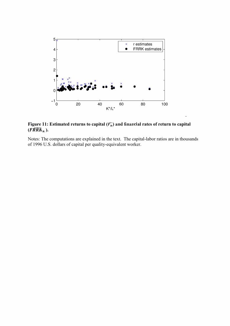
Figure 11: Estimated returns to capital ( ) and financial rates of return to capital( ).

Notes: The computations are explained in the text. The capital-labor ratios are in thousandsof 1996 U.S. dollars of capital per quality-equivalent worker.