capital structure and fair return on equity c2 tab 01... · principles of analysis for capital...
TRANSCRIPT
Filed: 2007-11-30 EB-2007-0905
Exhibit C2 Tab 1
Schedule 1 Page 1 of 261
Opinion
on
Capital Structure and Fair Return on Equity
Prepared for
ONTARIO POWER GENERATION
Prepared by
KATHLEEN C. McSHANE
FOSTER ASSOCIATES, INC.
November 2007
Filed: 2007-11-30 EB-2007-0905 Exhibit C2 Tab 1 Schedule 1 Page 2 of 261
TABLE OF CONTENTS
Page I. INTRODUCTION AND CONCLUSIONS 4
II. PRINCIPLES OF ANALYSIS FOR CAPITAL STRUCTURE AND RETURN ON EQUITY 10 A. THE FAIR RETURN STANDARD 10 B. THE STAND-ALONE PRINCIPLE 11 C. RELATIONSHIP BETWEEN CAPITAL STRUCTURE AND COST
OF CAPITAL 12 D. RATE BASE AND CAPITALIZATION 14
E. CAPITAL STRUCTURE: DEEMED VERSUS ACTUAL 15
III. BENCHMARK RETURN ON EQUITY 18 A. CONCEPT OF BENCHMARK RETURN 18 B. APPROACH TO ESTIMATION OF BENCHMARK RETURN
ON EQUITY 22 C. EQUITY RISK PREMIUM TESTS 23 D. DISCOUNTED CASH FLOW TEST 42 E. ALLOWANCE FOR FINANCING FLEXIBILITY 44 F. COMPARABLE EARNINGS TEST 46 G. FAIR RETURN ON EQUITY FOR A BENCHMARK
CANADIAN UTILITY 50
IV. DEEMED CAPITAL STRUCTURE FOR OPG REGULATED 52 A. PRINCIPLES 52 B. BUSINESS RISKS 55 C. IMPORTANCE OF INVESTMENT GRADE DEBT RATINGS 78 D. DEBT RATINGS OF OPG 81 E. FINANCIAL METRIC GUIDELINES 85 F. CAPITAL STRUCTURES OF PEERS 88 G. CAPITAL STRUCTURE FOR OPG AT BENCHMARK RETURN 91 H. RECOMMENDED CAPITAL STRUCTURE AND FAIR RETURN 96 I. IMPLIED CAPITAL STRUCTURE OF OPG’S UNREGULATED
OPERATIONS 97
Filed: 2007-11-30 EB-2007-0905
Exhibit C2 Tab 1
Schedule 1 Page 3 of 261
Page V. CAPITAL MARKET VIEWS ON FAIR RETURN/CAPITAL
STRUCTURE 99 A. IMPLICATIONS OF GLOBALIZATION OF CAPITAL MARKETS 99 B. VIEWS OF CANADIAN DEBT RATING AGENCIES 101 C. VIEWS OF EQUITY ANALYSTS 103 VI. AUTOMATIC ADJUSTMENT MECHANISM 107 APPENDICES: 111
A. DEEMED VERSUS ACTUAL CAPITAL STRUCTURE 113 B. THE CAPITAL ATTRACTION AND COMPARABLE
EARNINGS STANDARDS 124
C. RISK-ADJUSTED EQUITY MARKET RISK PREMIUM TEST 129
D. DCF-BASED RISK PREMIUM TEST 159 E. DISCOUNTED CASH FLOW TEST 161 F. COMPARABLE EARNINGS TEST 168 G. FINANCING FLEXIBILITY ADJUSTMENT 181 H. DEBT RATING AGENCY FINANCIAL METRIC
GUIDELINES 187
I. TRANSLATION OF RETURN REQUIREMENT TO COMMON EQUITY RATIO 189
J. QUALIFICATIONS OF KATHLEEN C. McSHANE 202 STATISTICAL EXHIBIT 209
Filed: 2007-11-30 EB-2007-0905 Exhibit C2 Tab 1 Schedule 1 Page 4 of 261
I. INTRODUCTION AND EXECUTIVE SUMMARY
A. INTRODUCTION
My name is Kathleen C. McShane and my business address is 4550 Montgomery Avenue, Suite
350N, Bethesda, Maryland 20814. I am President of Foster Associates, Inc., an economic
consulting firm. I hold a Masters in Business Administration with a concentration in Finance
from the University of Florida (1980) and the Chartered Financial Analyst designation (1989).
I have testified on issues related to cost of capital and various ratemaking issues on behalf of
local gas distribution utilities, pipelines, electric utilities and telephone companies, in more than
150 proceedings in Canada and the U.S. My professional experience is provided in Appendix J.
I have been requested by Ontario Power Generation Inc. (“OPG”) to recommend a capital
structure and fair return on equity for the Company’s prescribed assets. OPG’s prescribed assets
include six hydroelectric generating stations comprising 3332 MW of capacity and three nuclear
generation stations comprising 6606 MW of capacity.1
1 Regulated operations also include the costs and revenues from the lease arrangements between OPG and Bruce Power for the Bruce Nuclear Generating Stations.
Filed: 2007-11-30 EB-2007-0905
Exhibit C2 Tab 1
Schedule 1 Page 5 of 261
B. CONCLUSIONS
1. The return and capital structure for OPG’s regulated operations are governed by the fair
return standard.
2. A fair return for OPG’s regulated operations, which encompasses both capital structure
and return on equity, should respect the stand-alone principle.
3. OPG is entitled to the opportunity to earn a fair return on the assets that are devoted to,
and are used and useful in, the provision of regulated service, i.e., its rate base. An
original cost rate base should be used for purposes of determining the capital structure
and the application of the return on equity.
4. A deemed capital structure should be adopted for OPG because:
a. It is compatible with the premise that the allowed return should be based on the
stand-alone risk of the regulated operations,
b. It provides a means to implement the basic principle of finance that the higher the
business risk, the lower should be the debt ratio, and
c. OPG has significant non-regulated operations whose business risks and cost of
capital may be different from the risks and cost of capital of its regulated
business.
5. To estimate a reasonable return on equity and capital structure for OPG, I estimated the
return on equity that would be applicable to a benchmark (average risk) Canadian utility.
I subsequently estimated the deemed capital structure for OPG that:
a. Is compatible with its business risks;
b. Would permit it to achieve a stand-alone debt rating similar to that of the proxy
utilities used to establish the benchmark return; and,
Filed: 2007-11-30 EB-2007-0905 Exhibit C2 Tab 1 Schedule 1 Page 6 of 261
c. Would equate the level of total (business and financial) risk faced by OPG to that
of a benchmark (average risk) Canadian utility.
6. The benchmark return on equity was estimated at 10.25-10.75%. The fair return for a
benchmark utility reflects the following:
a. The return on equity is based on the results of three tests, equity risk premium,
discounted cash flow and comparable earnings.
b. The equity risk premium test results are based on three separate approaches. The
equity risk premium test supports the following return:
Risk-Free Rate 5.0%
Equity Risk Premium 4.25-5.25%
Financing Flexibility Adjustment 0.5%
Return on Equity 9.75-10.75%
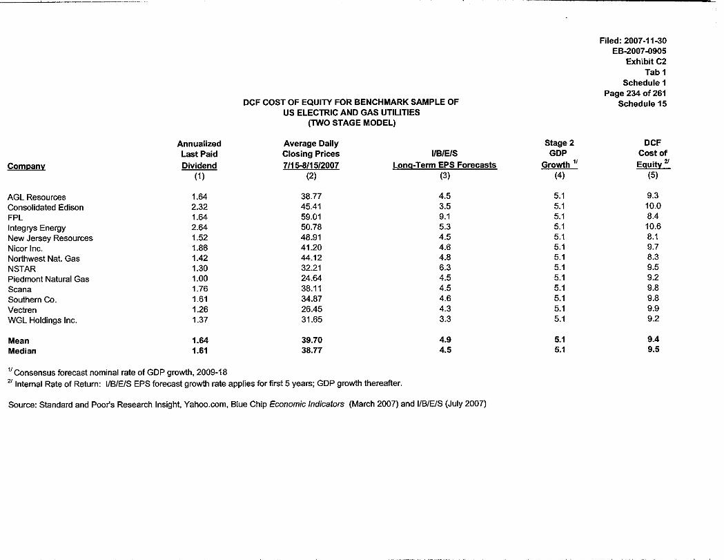
c. The discounted cash flow test, applied to a sample of benchmark low risk U.S.
utilities supports a cost of equity of 9.25-9.5%. With a 0.50% adjustment to the
“bare-bones” market cost of equity for financing flexibility, a fair return based on
the DCF test is 9.75-10.0%.
d. The comparable earnings test shows that, based on the achievable earnings returns
of low risk competitive non-regulated Canadian firms, a fair return applicable to a
benchmark utility would be approximately 12.5%.
e. With primary weight given to the two capital market tests, equity risk premium
and discounted cash flow, the fair return for a benchmark Canadian utility is
10.25-10.75% (mid-point of 10.5%).
7. A return of 10.5% is applicable to OPG’s regulated operations at a deemed common
equity ratio sufficient to equate their total risk (business and financial) to that of the
proxies used to estimate the benchmark return.
Filed: 2007-11-30 EB-2007-0905
Exhibit C2 Tab 1
Schedule 1 Page 7 of 261
8. The deemed capital structure for OPG should respect the following principles:
a. The stand-alone principle.
b. Compatibility of the capital structure with OPG’s business risks.
c. Maintenance of creditworthiness/financial integrity.
d. Compatibility with the benchmark return on equity.
9. With respect to relative business risk, OPG’s regulated operations face significantly
higher business risks than a benchmark average risk Canadian utility, or a low risk U.S.
utility.
10. To ensure access to the public debt markets, the capital structure for OPG’s regulated
operations should be sufficient to achieve debt ratings on a stand-alone basis in the A
category. The reasons for targeting an A rating include:
a. OPG is facing the potential of significant capital expenditures, for which it may
require public debt market access on reasonable terms and conditions. An A
rating will help ensure access on reasonable terms and conditions when the debt
capital is required.
b. The market for BBB rated debt in Canada remains relatively small, and is
particularly limited for long-term (i.e., 30 year) issues. OPG should have the
ability to access the long-term debt market to finance long-term assets.
c. The benchmark equity return recommended for OPG is intended to represent the
return applicable to an average risk, A rated, Canadian utility. Targeting an A
rating through the deemed capital structure ensures compatibility of the ROE and
capital structure.
11. The current DBRS and S&P debt ratings for OPG’s consolidated operations are based on
equity ratios in the range of 55-60%. Based on an analysis of the debt rating reports,
including the rating agencies’ assessment of the business risks of the regulated

Filed: 2007-11-30 EB-2007-0905 Exhibit C2 Tab 1 Schedule 1 Page 8 of 261
operations, the deemed common equity ratio for OPG’s regulated operations would need
to be in a similar range to maintain similar stand-alone debt ratings.
12. The quantitative guidelines of the debt rating agencies for a utility facing a similar
business risk profile to OPG’s regulated operations and an A debt rating support a
deemed common equity ratio in the range of 55-60%.
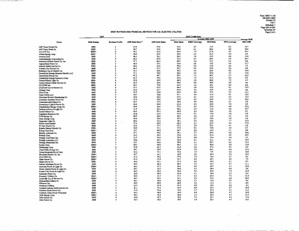
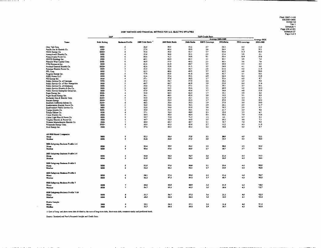
13. The average common equity ratio for the electric utility industry in North America is
approximately 45%, which, in conjunction with returns on equity in the 11-12% range, is
associated with a debt rating of BBB. The deemed common equity ratio for OPG at the
benchmark return on equity of 10.5% is premised on achieving an A rating. The deemed
equity ratio will need to be materially higher than the industry average of 45% to
notionally achieve an A debt rating.
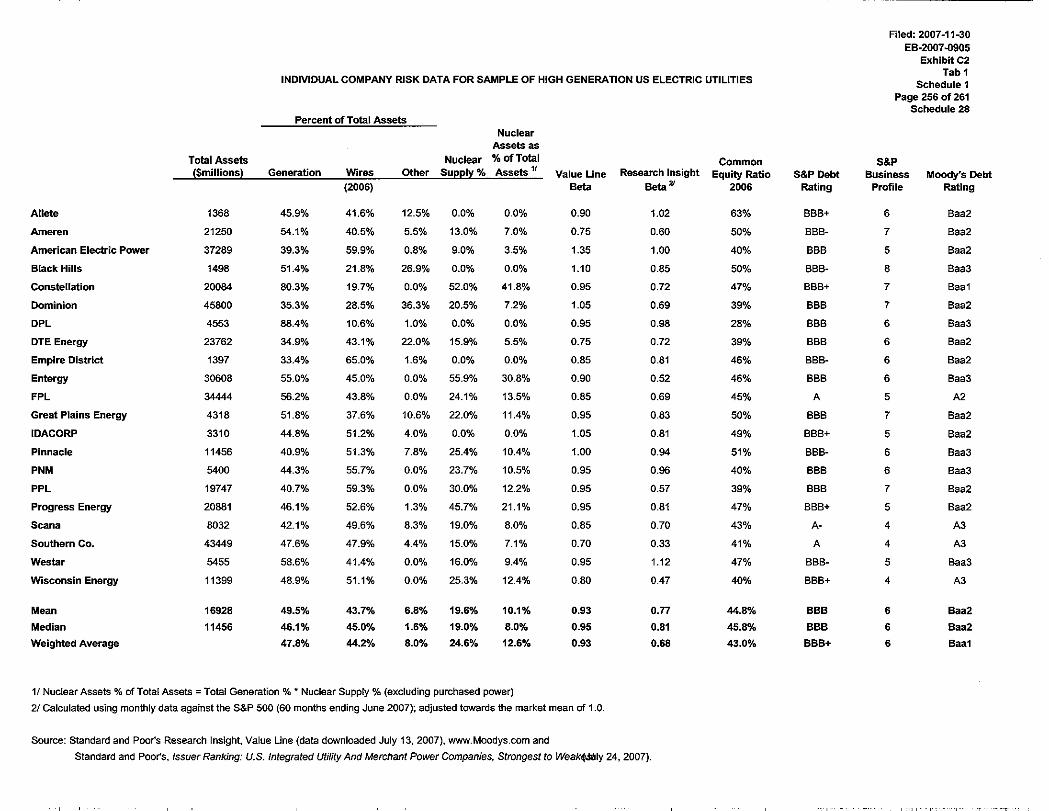
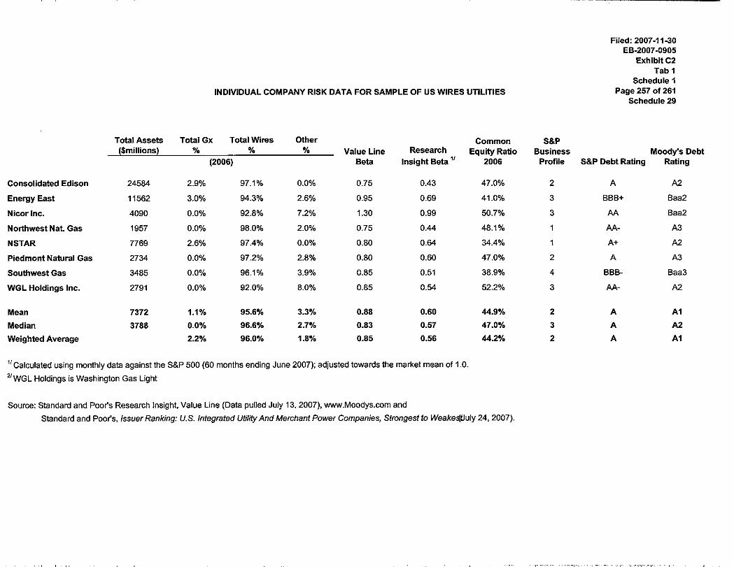
14. OPG’s regulated generation operations face higher business risk than the benchmark
utilities, which are largely “wires” or “pipes” companies. To estimate the common
equity ratio for OPG’s regulated operations that would permit the application of the
benchmark return of 10.5%, I estimated the incremental cost of equity for OPG from the
cost of equity for utilities with a high proportion of generation assets. From their cost of
equity, I also derived a generation-only cost of equity. The incremental costs of equity
for the “high generation” utilities and for generation-only were then translated into the
common equity ratio required to equate OPG’s total risk to that of a low risk benchmark
utility based on capital structure theory. The analysis, which takes account of the
application of two capital structure theories, indicates that the range of the required
common equity ratio for OPG’s regulated operations consistent with the benchmark
return is 55-60%.
Filed: 2007-11-30 EB-2007-0905
Exhibit C2 Tab 1
Schedule 1 Page 9 of 261
15. A review of capital market participants’ views indicates that the returns available to
comparable U.S. utilities are materially higher than the returns that are allowed to
Canadian utilities, the returns allowed for Canadian utilities are generally regarded as too
low, and the returns that investors expect and are achieving from the traded utility entities
in Canada are considerably higher than the returns that have been allowed by regulators.
These factors are legitimate considerations to be taken into account in setting a fair and
reasonable return for OPG’s regulated operations, and are supportive of the
recommended capital structure and return on equity.
16. I recommend the adoption of an automatic adjustment formula for return on equity for
OPG. Since OPG is facing multiple limited issue proceedings, with ROE assigned to the
first, the implementation of an automatic adjustment mechanism to operate until full
rebasing of regulated payments is complete is particularly warranted.
The Board’s existing formula, that is, a 75 basis point change in ROE for every one
percentage point change in forecast 30-year Canada bond yields is a reasonable reflection
of the relationship between the cost of equity and interest rates. However, the key to the
success of the formula is the initial adoption of a reasonable return on equity.
The automatic adjustment mechanism needs to preserve OPG’s right to seek a review of
the formula if OPG’s ability to attract capital on reasonable terms is at risk. In the
alternative, OPG should be able to seek a review of its deemed capital structure, should
its business risks change materially or its access to capital is threatened.
The formula should also be reviewed if forecast long Canada bond yields fall below 3.0%
or exceed 8.0%, as those extremes could signal a material change in the capital market
environment.
Filed: 2007-11-30 EB-2007-0905 Exhibit C2 Tab 1 Schedule 1 Page 10 of 261 II. PRINCIPLES OF ANALYSIS FOR CAPITAL STRUCTURE
AND RETURN ON EQUITY
A. THE FAIR RETURN STANDARD
The standards for a fair return arise from legal precedents2 which are echoed in numerous
regulatory decisions across North America.3 A fair return gives a regulated utility the
opportunity to:
1. earn a return on investment commensurate with that of comparable risk enterprises;
2. maintain its financial integrity; and,
3. attract capital on reasonable terms.
A fair return on the capital provided by investors not only compensates the investors who have
put up, and continue to commit, the funds necessary to deliver service, but benefits all
stakeholders, including ratepayers. A fair and reasonable return on the capital invested provides
the basis for attraction of capital for which investors have alternative investment opportunities.
Fair compensation on the capital committed to the utility provides the financial means to pursue
technological innovations and build the infrastructure required to support long-term growth in
the underlying economy.
2 The principal court cases in Canada and the U.S. establishing the standards include Northwestern Utilities Ltd. v. Edmonton (City), [1929] S.C.R. 186; Bluefield Water Works & Improvement Co. v. Public Service Commission of West Virginia,(262 U.S. 679, 692 (1923)); and, Federal Power Commission v. Hope Natural Gas Company (320 U.S. 591 (1944)). 3 In EB-2005-0421(Toronto Hydro), dated April 12, 2006, the OEB stated, “And, as a matter of law, utilities are entitled to earn a rate of return that not only enables them to attract capital on reasonable terms but is comparable to the return granted other utilities with a similar risk profile.” (pages 32-33)

Filed: 2007-11-30 EB-2007-0905
Exhibit C2 Tab 1
Schedule 1 Page 11 of 261
An inadequate return, on the other hand, undermines the ability of a utility to compete for
investment capital. Moreover, inadequate returns act as a disincentive to expansion, may
potentially degrade the quality of service or deprive existing customers from the benefit of lower
unit costs that might be achieved from growth. In short, if the utility is not provided the
opportunity to earn a fair and reasonable return, it may be prevented from making the requisite
level of investments in the existing infrastructure in order to reliably provide utility services for
its customers. The OEB has recognized the importance of a financially viable energy sector and
the need for additional energy infrastructure, particularly generation and transmission, in its
Strategic Business Objectives set out in its 2006-2009 Business Plan (December 2005). Fair and
reasonable returns are central to the achievement of those objectives.
B. THE STAND-ALONE PRINCIPLE
A fair return for OPG's regulated operations, which encompasses both capital structure and
return on equity, should respect the stand-alone principle. The stand-alone principle has been
respected by virtually every Canadian regulator, including the OEB, in setting both regulated
capital structures and allowed returns on equity.
The stand-alone principle is the notion that the cost of capital incurred by ratepayers should be
equivalent to that which would be faced by the regulated operations if they were raising capital
in the public markets on the strength of their own business and financial parameters. In other
words, application of the stand-alone principle to OPG’s regulated operations means they should
be treated for regulatory purposes as if they were operating separately from the other activities of
the firm. The cost of capital borne by ratepayers should reflect neither subsidies given to, nor
taken from, other activities of the firm.
The evaluation of the appropriate capital structure and common equity return on a “stand-alone”
basis avoids: (1) the misconception that the cost of raising capital to invest in a project (the
financing decision) is the same as the cost of capital (required return) of the project (the

Filed: 2007-11-30 EB-2007-0905 Exhibit C2 Tab 1 Schedule 1 Page 12 of 261 investment decision); and (2) the potential that hidden subsidies created by using an
inappropriate cost of capital can distort the economics of the project itself. To illustrate, the
Federal Government can raise long-term debt at relatively low interest rates because its taxing
power assures the cash flows needed to reimburse investors. If the Federal Government were to
consider investing either in natural gas exploration and development or a water utility, its
evaluation of the two potential investments should be based on required returns that reflect the
different business risks of the two projects, not the cost to the Federal Government of raising
debt to finance its investment. A failure to do so, that is a failure to respect the “stand-alone”
principle, could lead to the erroneous conclusion that the oil and gas development project was the
superior project and thus to an uneconomic allocation of capital resources. Effectively, the
Federal Government would be subsidizing natural gas exploration and development, while
potentially allowing a superior project to fail to attract investment funds. Respect for the stand-
alone principle ensures that scarce capital resources are efficiently allocated to their best use.
The allowed return should thus represent the stand-alone risk and associated cost of capital of the
operations, not the happenstance of ownership.
C. RELATIONSHIP BETWEEN CAPITAL STRUCTURE AND COST OF CAPITAL
The stand-alone principle is grounded in the basic tenet of financial theory that the opportunity
cost of capital to a firm, or division of a firm, is a function of its business risk. Business risk
comprises the operating elements of the business that together determine the probability that
future returns to investors will fall short of their expected and required returns. Business risk is a
function of the fundamental characteristics of the operations, i.e., of the firm’s assets. In the
absence of income taxes and the added costs related to the loss of financial flexibility and
financial distress or ultimately bankruptcy, the overall cost of capital would not change as the
manner in which it was financed changed. The cost of capital would be the same if a firm were
financed with 100% equity or 100% debt. In the absence of income taxes, the sum of the cash
flows, available to both the debt holders and equity holders does not change as the capital

Filed: 2007-11-30 EB-2007-0905
Exhibit C2 Tab 1
Schedule 1 Page 13 of 261
structure changes. However, the use of debt creates a class of investors whose claims on the
cash flows of the firm take precedence over those of the equity holder. Since the issuance of
debt carries unavoidable servicing costs which must be paid before the equity shareholder
receives any return, the potential variability of the equity shareholder’s return rises as more debt
is added to the capital structure. Thus, as the debt ratio rises, the cost of equity rises, but the
overall cost of capital is constant.
However, two factors alter the conclusion that the cost of capital stays constant as the capital
structure changes. First, the facts that (1) debt is less expensive than equity because debt
investors take precedence over equity investors, and (2) interest expense on debt is deductible for
corporate income tax purposes means that there is a cost advantage to using debt. Thus,
financing with a combination of debt and equity can lower the overall (weighted average) cost of
capital. Second, and partly offsetting the cost advantage of adding debt, are the additional costs
that are incurred as more debt is added to the capital structure. As the debt in the capital
structure increases, additional costs are incurred in the form of loss of financial flexibility and
financial distress, e.g., more stringent debt covenants, restrictions on the amount and term of debt
the market is willing to accept, and a decreased ability to access the market at the time funds are
required. These additional costs negatively impact not only explicit costs of debt and equity
financing, but can ultimately impact the ability to operate the business efficiently. As a result,
too much debt will increase the weighted average cost of capital, as the costs of financial distress
will outweigh the benefits of additional debt.
Two other factors can offset some of the advantage of using debt in the capital structure. The
first factor is the impact of personal income taxes on interest income. While interest expense is
deductible at the corporate level, the corresponding interest income is taxable to individual
investors at higher rates than equity income. Second, in the case of utilities, the benefits of the
tax deductibility of interest expense flow to ratepayers, not shareholders, as the utility revenue
requirement is reduced to reflect the lower income tax expense. (In contrast, for unregulated
Filed: 2007-11-30 EB-2007-0905 Exhibit C2 Tab 1 Schedule 1 Page 14 of 261 companies, the benefits of interest expense deductibility will flow to equity shareholders in the
form of a higher return.)
In theory, when all these factors are taken into account, there should be an optimal capital
structure, i.e., one that minimizes the overall cost of capital. In practice, the interactions of the
various factors make the optimal capital structure impossible to pin-point, and there exists a
range of capital structures over which the average cost of capital does not change materially.
Within this range, an increase in the debt ratio will result in an increase in both the cost of debt
and the cost of equity, but the overall cost of capital will not change measurably. A key message
is that the capital structure and the required return on equity are inter-dependent: As the debt
ratio of the regulated operations rises, the cost of equity also rises. That relationship needs to be
reflected in OPG’s capital structure and allowed return on equity.
D. RATE BASE AND CAPITALIZATION
Under the fair return standard, a utility is entitled to the opportunity to earn a fair return on the
investor-supplied capital that finances the assets that are devoted to, and are used and useful in,
the provision of regulated service. The rate base represents the measurement of the assets that
are used and useful in the delivery of public utility service; it corresponds to the amount of
capital that has been provided by investors and upon which investors are allowed the opportunity
to earn a fair return.
The most prevalent construct for measuring rate base in North America is a historic cost model,
often referred to as “original cost rate base.” Under the original cost methodology, the rate base
is measured using the cost of the assets at the time they are first devoted to public service. When
an original cost rate base is used, the return on rate base reflects the embedded cost of debt and a
nominal (inclusive of inflation) return on equity. The domination of original cost ratemaking
Filed: 2007-11-30 EB-2007-0905
Exhibit C2 Tab 1
Schedule 1 Page 15 of 261
reflects the results of more than half a century of regulatory and court decisions.4 Virtually every
regulated utility in Canada relies on an original cost rate base for purposes of determining the
allowed return on capital.
While the benefits of alternative models for rate base determination continue to be debated in
North America from time to time, there is no evidence that the original cost methodology for rate
base valuation would preclude utilities from attracting capital on reasonable terms and conditions
or from earning a return that is comparable to that of similar risk enterprises as long as the level
of the return itself recognizes the manner in which the rate base is measured. Moreover, the
requirement that the OEB accept the financial statement asset and liability values of OPG as per
Regulation 53/05 effectively eliminates from consideration any of the methodologies that are not
derived from original cost (e.g., reproduction or replacement cost).
E. CAPITAL STRUCTURE: DEEMED VERSUS ACTUAL5
As indicated in Chapter II.C, the cost of capital to the utility is a function of business risk. It is
also a function of financial risk. Financial risk refers to the additional risk that is borne by the
equity shareholder because the firm is using fixed income securities – debt and preferred shares
to finance a portion of its assets. The capital structure, comprised of debt, preferred share and
common equity, can be viewed as a summary measure of the financial risk of the firm. While
there is no universal agreement whether a single optimal capital structure for a firm exists, there
is agreement that, as a general proposition, companies with less business risk can safely assume
more debt than those with higher business risk without impairing their ability to access the
capital markets on reasonable terms and conditions. In principle, higher business risk can be
“offset” by assuming less financial risk. Thus, two utilities with different levels of business risk 4 Original cost rate base became the standard after the watershed U.S. Supreme Court decision, Federal Power Commission v. Hope Natural Gas (320 U.S. 391 (1944)), which addressed the controversy between original cost and fair value. In its decision, the Court held that it is the end result, not the method employed to value the rate base that is important. As a result of the Court’s findings in Hope, the original cost rate base became the standard, and the focus of regulation shifted from the valuation of the rate base to the fairness of the rate of return and the end result. 5 Appendix A contains more detail on the history of, and issues related to, deemed capital structures.
Filed: 2007-11-30 EB-2007-0905 Exhibit C2 Tab 1 Schedule 1 Page 16 of 261 can face similar costs of debt and equity if the utility facing higher business risk maintains a
lower debt ratio than the utility facing lower business risk.
The concept of a deemed, or hypothetical, capital structure can be viewed as a means of imputing
for regulatory purposes a level of financial risk that is “consistent” or “compatible” with the level
of business risk that a utility faces. The term “deemed capital structure” simply refers to the
imputation, for ratemaking purposes, of a capital structure that is different from the actual or
reported capital structure as derived from the utility’s financial statements. A deemed capital
structure is typically applied by estimating the rate base, applying a specified percentage of
common equity to the rate base, assigning to the rate base actual outstanding and forecast issues
of long-term debt and preferred shares, and then, to the extent that the capital structure does not
equal the rate base, “deem” the gap to be debt.
I recommend the adoption of a deemed capital structure for OPG’s regulated operations.6 The
principal reasons for this recommendation are as follows:
1. Using a deemed capital structure is consistent with basing the allowed return on an
opportunity cost of capital that reflects the use of funds (the risks of the operations to
which the funds are committed), rather than the source of those funds.
2. Using a deemed capital structure is consistent with regulatory practice (consistent with
financial theory) of adherence to the stand-alone principle as followed by Canadian
regulators, including the OEB, in setting the allowed return on rate base.
3. Using a deemed capital structure allows the general principle to be applied that the higher
is the regulated operations’ business risk, the lower the debt ratio should be. Recognizing 6 Issues relating to the specification of the appropriate deemed capital structure for OPG’s regulated operations are addressed in Chapter IV.
Filed: 2007-11-30 EB-2007-0905
Exhibit C2 Tab 1
Schedule 1 Page 17 of 261
the level of the regulated operations’ business risks primarily through the allowed capital
structure is a reasonable and accepted regulatory approach for differentiating among
utilities and compensating them for differences in business risk.
4. OPG has significant non-regulated operations whose business risks and cost of capital
may be different from the risks and cost of capital of its regulated business.
5. The use of a deemed capital structure provides assurance that ratepayers are protected
from any negative impacts on the consolidated firm’s cost of capital of unregulated
operations.
Filed: 2007-11-30 EB-2007-0905 Exhibit C2 Tab 1 Schedule 1 Page 18 of 261
III. BENCHMARK RETURN ON EQUITY A. CONCEPT OF BENCHMARK RETURN ON EQUITY
As indicated in Chapter II, the cost of equity is a function of both business and financial risk.
Financial risk, in turn, is a function of capital structure; the lower the common equity ratio, the
higher is the financial risk and the higher is the cost of equity. When a utility is regulated on the
basis of its actual capital structure or a previously approved deemed capital structure, its
financial risk must be addressed through the return on equity. The fair return for a utility with a
“fixed” capital structure would then be determined by (1) selecting a sample or samples of proxy
companies of relatively similar business risk to the utility; (2) estimating the samples’ cost of
equity; (3) quantifying any difference in equity return requirement between the utility and the
proxies due to differences in their capital structure; and (4) applying the financial-risk adjusted
return on equity to the utility. However, for OPG both an appropriate deemed capital structure
and fair return need to be determined. In setting the two values simultaneously, two basic
principles need to be recognized. First, the higher the business risk that a utility faces, the lower
would be an appropriate debt component, that is, one that would ensure the utility’s ability to
attract capital on reasonable terms and conditions. Second, the higher the debt component that is
chosen for a regulated firm facing a given level of business risk, the higher would be the cost of
equity and the reasonable allowed return on equity.
It is not possible to identify close proxies with equity market data, particularly within the
Canadian capital market context, that can be used to directly estimate either a reasonable capital
structure or the cost of equity for OPG’s regulated operations, for two reasons. First, OPG’s
regulated operations are unique. Second, there are a very limited number of publicly-traded
regulated companies in Canada. In the absence of Canadian proxies of similar risk to OPG, there
Filed: 2007-11-30 EB-2007-0905
Exhibit C2 Tab 1
Schedule 1 Page 19 of 261
are essentially two approaches that can be used. The first approach entails estimating and
applying to OPG the equity return that would be applicable to a “benchmark” or average risk
Canadian utility. That return will be referred to as a “benchmark return”. A deemed capital
structure for OPG would then be determined that (a) is compatible with its business risks; (b)
would permit it to achieve a stand-alone debt rating similar to that of proxy companies used to
establish the benchmark return; and (c) would equate the level of total (business and financial)
risk faced by OPG to that of the proxies used to estimate the benchmark cost of equity. Under
this approach, the benchmark return on equity is “fixed” and the deemed common equity ratio
for OPG’s regulated operations established so that no adjustment to the benchmark return on
equity is required.7
The second approach sets the deemed capital structure first, relying on factors such as debt rating
agency guidelines for an investment grade debt rating and capital structure ratios maintained by
peers in the industry. This approach entails establishing a deemed common equity ratio that is
reasonable, but would not necessarily equate OPG’s total (business plus financial) risk to that of
a benchmark utility. In the implementation of this approach, OPG’s total risks would be
compared to those of the proxy firms used to establish the benchmark. If OPG’s total risk, at the
specified deemed common equity ratio is higher than that of the benchmark utility, the
incremental equity return requirement needs to be estimated and added to the return on equity
applicable to a benchmark utility. The key difference between the first and second approaches is
that in the second, both capital structure and return on equity are essentially “moving parts.”
Because there are so few publicly-traded utilities in Canada, both approaches rely on the
measurement of a benchmark return on equity as a point of departure for estimating the return on
equity applicable to a particular utility.
7 In this regard, Standard & Poor’s notes that the business and financial risk components are inextricable. “For example, a utility with a strong business profile could have less financial protection than one with a weaker business profile, yet they could still achieve the same rating. Conversely, a utility with a weak business profile could require a more robust financial profile than one with a stronger business profile in order to get the same rating.” Standard & Poor’s, Research: Rating Methodology for Global Power Utilities, August 30, 1999.
Filed: 2007-11-30 EB-2007-0905 Exhibit C2 Tab 1 Schedule 1 Page 20 of 261 The term “benchmark utility” is a hypothetical construct, because it does not refer to a specific
utility and hence reflects no specific business or financial risks. Since the estimate of the cost of
equity is derived from market data for utilities across industries (electric, gas distribution and gas
pipeline), the “benchmark utility” reflects, in effect, the composite of the business and financial
risks faced by the utilities used to establish the benchmark return. However, one objective
measure of what constitutes a benchmark utility would be its ability, on a stand-alone basis, to
achieve debt ratings in the A category. The typical, average risk, Canadian utility is rated in the
A category by both of the major debt rating agencies, DBRS and Standard & Poor’s.
Designation of the debt rating as an indicator of relative risk recognizes that (1) debt ratings
reflect both business and financial risk, and (2) the equity return requirement is a function of
both business and financial risk. Thus, the benchmark return on equity would be one that is
applicable to a specific utility whose capital structure is adequate to achieve, on a stand-alone
basis, debt ratings in the A category (See Chapter IV.C for reasons). The estimation of the
benchmark return on equity must then be derived from proxy groups whose total risk permits
them to achieve debt ratings in the A category.
Both of the approaches described above have been taken by regulators in Canada. The first
approach was employed by the National Energy Board (NEB) when it established its automatic
adjustment mechanism for a number of oil and gas pipelines in 1995. The individual pipelines
were deemed capital structure ratios that were intended to compensate for their different levels of
business risks, so that a single “benchmark” return on equity could be applied across all of the
pipelines. In the years since the multi-pipeline return on equity was adopted, the NEB has
changed the allowed capital structure, rather than the allowed return, to recognize changes in
business risk.
It is also the approach that was adopted by the Alberta Energy and Utilities Board (AEUB) in
Decision 2004-052 (July 2, 2004). In that decision, the AEUB set different capital structures for
eleven electric and gas distribution and transmission entities, based on their different business
Filed: 2007-11-30 EB-2007-0905
Exhibit C2 Tab 1
Schedule 1 Page 21 of 261
risk profiles, and then established a common return on equity to be applied to each of the utilities
under its jurisdiction.
In contrast to the NEB and AEUB approach, the British Columbia Utilities Commission has
allowed for both different capital structures and different equity risk premiums among the
various utilities it regulates. The Commission explicitly specifies the low risk benchmark return
on equity; each utility’s risk premium is expressed in relationship to the low risk benchmark risk
premium. It also has designated one utility (Terasen Gas) as the low risk benchmark utility.
In Ontario, the OEB has used both approaches. For the two large gas distribution utilities, the
Board historically had approved the same deemed common equity ratios for Enbridge Gas
Distribution and Union Gas and allowed a somewhat higher equity risk premium for Union Gas.
As a result of its recent settlement (RP-2005-0520, June 29, 2006), Union Gas currently has a
somewhat higher equity risk premium and a one percentage point higher deemed common equity
ratio. As a result of the Board’s Reasons for Decision in EB-2005-0544 (September 20, 2006),
Natural Resource Gas is allowed a higher common equity ratio and a higher equity risk premium
than either Enbridge or Union. For the electricity distribution utilities, from 2000-2006 the
Board allowed a range of deemed common equity ratios using size of rate base as the
distinguishing risk factor and applied the same return on equity to each of the utilities.
In my opinion, both approaches are valid as long as the combination of capital structure and
return on equity for a particular utility reasonably compensates for the shareholders for the
utility’s combined business risk and financial risks relative to that of its peers.
For OPG, I have relied on the approach that was adopted by the OEB for electricity distributors
in 2000, and by the NEB (1995) and AEUB (2004). Specifically, I estimated a benchmark return
on equity and then determined the deemed capital structure for OPG’s regulated operations that
is compatible with its business risks, would permit it to achieve the same debt rating on a stand-

Filed: 2007-11-30 EB-2007-0905 Exhibit C2 Tab 1 Schedule 1 Page 22 of 261 alone basis as the utilities used to estimate the benchmark return, and would equate its level of
total business and financial risks to those of the proxy samples.
B. APPROACH TO ESTIMATION OF BENCHMARK RETURN ON
EQUITY
To ensure that the allowed return considers all of the relevant factors that bear on a fair return, I
recommend application of the three tests that have traditionally been used to set a fair return for
regulated companies: the equity risk premium test, the discounted cash flow test and the
comparable earnings test. Reliance on multiple tests recognizes that no one test produces a
definitive estimate of the fair return.8 Each test is a forward-looking estimate of investors’ equity
return requirements. However, the premises of each of the three tests differ; each test has its
own strengths and weaknesses. In principle, the concept of a fair and reasonable return does not
reduce to a simple mathematical construct. It would be unreasonable to view it as such.
Moreover, the three criteria that define a fair return, set forth in Chapter II.A, give rise to two
separate standards, the capital attraction standard and the comparable returns, or comparable
earnings, standard. A fair and reasonable return gives weight to both the cost of attracting capital
Standard and comparable earnings standard.9 The two standards are applied using different tests.
The equity risk premium and discounted cash flow tests establish the cost of attracting capital.
The comparable earnings test is a measure of the comparable return, or comparable earnings,
standard. To establish the benchmark return on equity, I have applied all three. The application
of each of the tests is discussed in the sections below.
8 As stated in Bonbright, “No single or group test or technique is conclusive.” (James C. Bonbright, Albert L. Danielsen, David R. Kamerschen, Principles of Public Utility Rates, 2nd Ed., Arlington, Va.: Public Utilities Reports, Inc., March 1988). 9 Appendix B discusses the distinctions between the two standards.
Filed: 2007-11-30 EB-2007-0905
Exhibit C2 Tab 1
Schedule 1 Page 23 of 261
C. EQUITY RISK PREMIUM TESTS
C.1. Conceptual Underpinnings
The equity risk premium test is derived from the basic concept of finance that there is a direct
relationship between the level of risk assumed and the return required. Since an investor in
common equity takes greater risk than an investor in bonds, the former requires a premium above
bond yields in compensation for the greater risk. The equity risk premium test is a measure of
the market-related cost of attracting capital, i.e., a return on the market value of the common
stock, not the book value.
The equity risk premium test, similar to the other tests used to arrive at a fair return, is forward-
looking, that is, it is intended to estimate investors’ future equity return requirements. The
magnitude of the differential between the required/expected return on equities and the risk-free
rate is a function of investors’ willingness to take risks10 and their views of such key factors as
inflation, productivity and profitability. Because the risk premium test is forward-looking,
historic risk premium data need to be evaluated in light of prevailing economic/capital market
conditions. If available, direct estimates of the forward-looking risk premium should supplement
estimates of the risk premium made using historic data as the point of departure.
10 To illustrate, equity market volatility has picked up significantly in 2007, as investors have become less sanguine about the future of the equity market, in light of the recent housing market and sub-prime mortgage market crises. The VIX index, an equity volatility index calculated by the Chicago Board Option Exchange (often referred to as the “Fear Gauge”), indicates that, during much of 2004-2006, the equity market was perceived as unusually stable; that is no longer the case. The VIX index has been rising throughout 2007, increasing by approximately 150% from the beginning of the 2007 to the middle of the 4th Quarter, with much of the increase in the latter half of the year. During November of 2007, the VIX index reached its highest levels since 2003. An increase in the VIX index signals rising risk aversion and an increase in the required equity risk premium.
Filed: 2007-11-30 EB-2007-0905 Exhibit C2 Tab 1 Schedule 1 Page 24 of 261 C.2. Risk-Free Rate
The application of the equity risk premium tests requires a forecast of the risk-free rate to which
the equity risk premium is applied. Reliance on a long-term government bond yield as the risk-
free rate recognizes (1) the administered nature of short-term rates; and (2) the long-term nature
of the assets to which the equity return is applicable. The risk-free rate, for purposes of this
analysis, is the forecast 30-year Canada yield which is based on the consensus forecast for 10-
year Canada bonds plus the spread between 10- and 30-year Canada bond yields.11 Consensus
Forecasts, Consensus Economics (August 13, 2007) anticipates that the 10-year yield will be
approximately 4.7% by November 2007 and 5.0% by August 2008 (average of 4.85).
At the end of August 2007, the yield curve was relatively flat; the yields on 10- and 30-year
bonds were only approximately 10 basis points apart. On average, historically, the spread has
been a positive 30 basis points, reflecting a normal upward sloping yield curve. For purposes of
applying the equity risk premium test for the test period, I have estimated the 30-year Canada
bond yield at approximately 5.0%, reflecting a continuation of a relatively flat yield curve.12
C.3. Risk-Adjusted Equity Market Risk Premium Test
C.3.a. Conceptual and Empirical Considerations
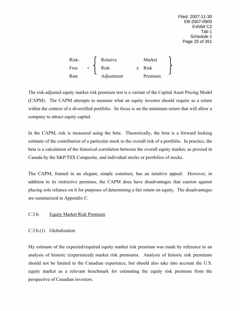
The risk-adjusted equity market risk premium approach to estimating the required utility equity
risk premium entails (1) estimating the equity risk premium for the equity market as a whole; (2)
estimating the relative risk adjustment required for a benchmark Canadian utility; and (3)
applying the relative risk adjustment to the equity market risk premium, to arrive at the equity
risk premium required for a benchmark Canadian utility. The cost of equity is thus estimated as:
11 There is no consensus forecast of 30-year Canadian bond yields. 12 The long-term Canada bond yield (and resulting ROE) will be updated for the most recent available forecast prior to the hearing.
Filed: 2007-11-30 EB-2007-0905
Exhibit C2 Tab 1
Schedule 1 Page 25 of 261
Risk-
Free
Rate
+
Relative
Risk
Adjustment
x
Market
Risk
Premium
The risk-adjusted equity market risk premium test is a variant of the Capital Asset Pricing Model
(CAPM). The CAPM attempts to measure what an equity investor should require as a return
within the context of a diversified portfolio. Its focus is on the minimum return that will allow a
company to attract equity capital.
In the CAPM, risk is measured using the beta. Theoretically, the beta is a forward looking
estimate of the contribution of a particular stock to the overall risk of a portfolio. In practice, the
beta is a calculation of the historical correlation between the overall equity market, as proxied in
Canada by the S&P/TSX Composite, and individual stocks or portfolios of stocks.
The CAPM, framed in an elegant, simple construct, has an intuitive appeal. However, in
addition to its restrictive premises, the CAPM does have disadvantages that caution against
placing sole reliance on it for purposes of determining a fair return on equity. The disadvantages
are summarized in Appendix C.
C.3.b. Equity Market Risk Premium
C.3.b.(1) Globalization
My estimate of the expected/required equity market risk premium was made by reference to an
analysis of historic (experienced) market risk premiums. Analysis of historic risk premiums
should not be limited to the Canadian experience, but should also take into account the U.S.
equity market as a relevant benchmark for estimating the equity risk premium from the
perspective of Canadian investors.

Filed: 2007-11-30 EB-2007-0905 Exhibit C2 Tab 1 Schedule 1 Page 26 of 261
The historic Canadian equity and government bond returns incorporate various factors that make
them questionable as a realistic representation of future risk premiums (e.g., capital held captive
in Canada as a matter of policy, lack of equity market liquidity and diversity, and the higher risk
of the Government of Canada bond market historically, which has since dissipated).
Of particular importance has been the historic impact of the Foreign Property Rule (FPR), which
capped the proportion of foreign investment that could be held by individuals (in RRSPs) and by
pension funds. The combination of mediocre returns and small size of the Canadian market
relative to the total global market (approximately 2%) put pressure on the government to increase
and finally eliminate the cap on foreign investment that could be held in RRSPs and pension
funds. This cap has been as low as 10% of the book value of assets (from 1971 to 1990) and was
at 30% when it was removed entirely in August 2005 effective January 1, 2005.13 Historic
Canadian equity returns therefore are likely to understate investor return requirements.
The investor reaction to the increasingly less restrictive FPR supports that conclusion. Equity
investment outside of Canada has grown rapidly as the barriers to foreign investment (in terms of
both transactions and information costs as well as the foreign investment cap) have declined.
Foreign stock purchases by Canadians have increased over seven-fold over the past decade.
Purchases in 1995 were $83 billion; in 2006, they were $570 billion.14 In 2006, although the
total percentage of foreign assets in the top 100 Canadian pension funds was only 33%, the
percentage of foreign equity to total equity was close to 56%.15 While the FPR was in effect,
pension funds concentrated their foreign investment allocations to the equity markets, with the
preponderance of their fixed income allocations to domestic bonds. 13 From 1957 to 1971 no more than 10% of income could come from foreign sources. 14 The IFIC’s report “Year 2002 in Review” stated,
During the period of 1991-1998, the percentage of sales in equity mutual funds that were comprised of non-domestic equities has hovered around the 41-58% range. This has significantly increased in 1999 and onwards. While performance in the markets is the major factor affecting such an increase, these figures can also be attributed to increases in foreign content limits in registered retirement savings plans as well as increased interest and availability of foreign clone funds.
15 Benefits Canada, “2007 Top 100 Pension Funds”, May 2007.
Filed: 2007-11-30 EB-2007-0905
Exhibit C2 Tab 1
Schedule 1 Page 27 of 261
The relevance of the U.S. experience to the estimation of the risk premium from a Canadian
perspective has increased as the relationship between Canadian and U.S. interest rates has
changed. From 1947-2006, the achieved risk premiums in Canada were 140 basis points lower
than in the U.S. Of that amount, approximately 80 basis points are accounted for by historically
higher bond yields in Canada. With the vastly improved economic fundamentals in Canada (e.g.,
lower inflation, balanced budgets), the risk of investing in Canadian government bonds has
declined. Consequently, the differential between Canadian and U.S. government bonds that
existed historically, on average, is not expected to persist in the future.
The most recent consensus of long-term forecasts of government bond yields anticipates that
yields will be slightly lower in Canada than in the U.S. in the future. Consensus Economics,
Consensus Forecasts, April 2007 anticipates an average 10-year government bond yield over the
period 2009-2017 of 5.1% for Canada and 5.25% for the U.S.16 With lower interest rates in
Canada, the differential between equity and bond returns in the two countries should, ceteris
paribus, be closer in the future than it was historically. Consequently, the U.S. historic equity
market risk premium is a relevant benchmark in the estimation of the forward-looking equity
market risk premium for Canadian investors.
On the equity side of the equation, the Canadian equity market composite is dominated by two
sectors, financial services and energy. These two sectors alone accounted for approximately
58% of the total market capitalization of the S&P/TSX Composite at the end of August 2007. In
contrast to the S&P/TSX Composite, the historic U.S. equity returns have been generated by a
more diversified and liquid market. In addition, the U.S. equity market has historically been the
principal alternative for Canadian investors to domestic equity investments. Approximately 50%
of Canadian portfolio investment in foreign equities at the end of 2006 was in the U.S.17 The
16 Blue Chip Financial Forecasts (June 2007), which canvasses economic forecasters at over 50 North American financial institutions, anticipates a 10-year U.S. Treasury yield of 5.15% from 2008-2017. 17 Source: Statistics Canada, Canada’s International Investment Position – First Quarter 2007. Of the remaining 51%, the next largest allocation of foreign portfolio equity investment is the U.K., which accounted for 13%.

Filed: 2007-11-30 EB-2007-0905 Exhibit C2 Tab 1 Schedule 1 Page 28 of 261 diversified nature of the U.S. equity market and the close relationship between the Canadian and
U.S. capital markets and economies warrant giving significant weight to U.S. historical equity
risk premiums in the estimation of the required equity risk premium for a benchmark Canadian
utility.
C.3.b.(2) The Post-World War II Period
The estimation of the expected/required market risk premium from achieved market risk
premiums is premised on the notion that investors’ return expectations and requirements are
linked to their past experience. Basing calculations of achieved risk premiums on the longest
periods available reflects the notion that it is necessary to reflect as broad a range of event types
as possible to avoid overweighting periods that represent “unusual” circumstances. On the other
hand, the objective of the analysis is to assess investor expectations in the current economic and
capital market environment. Consequently, I focused on post-World War II returns, that is,
1947-2006, a period more closely aligned with what today’s investors are likely to anticipate
over the longer-term.18
C.3.b.(3) Historic Risk Premiums
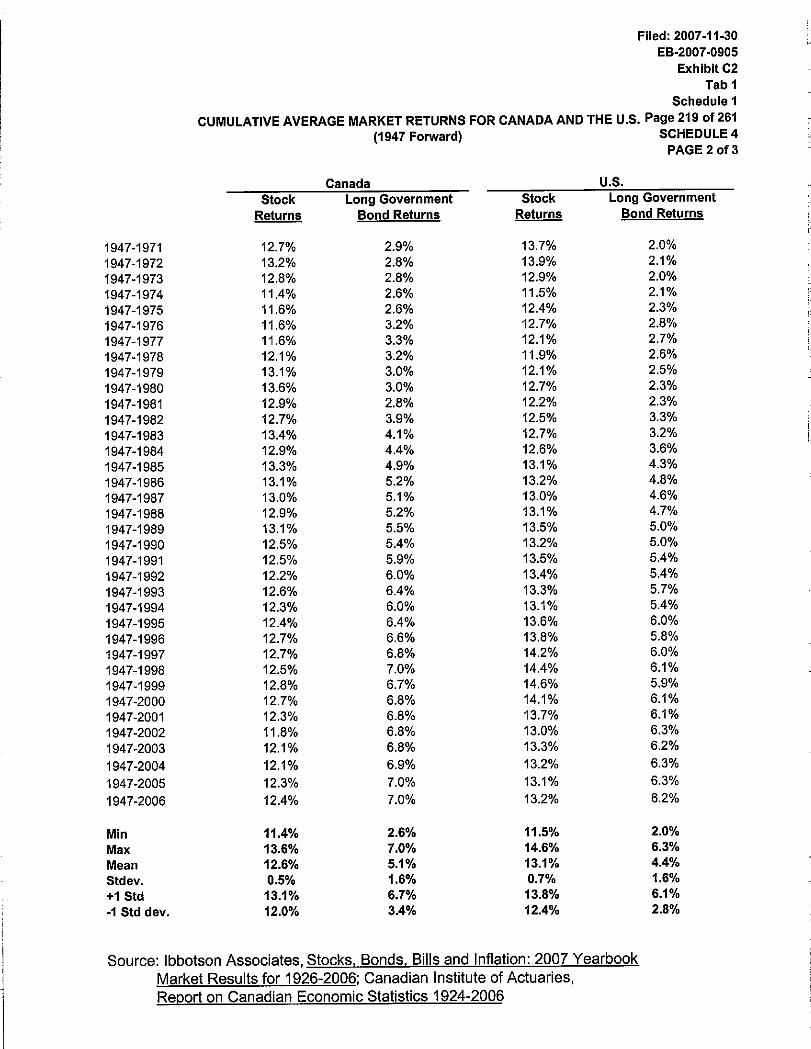
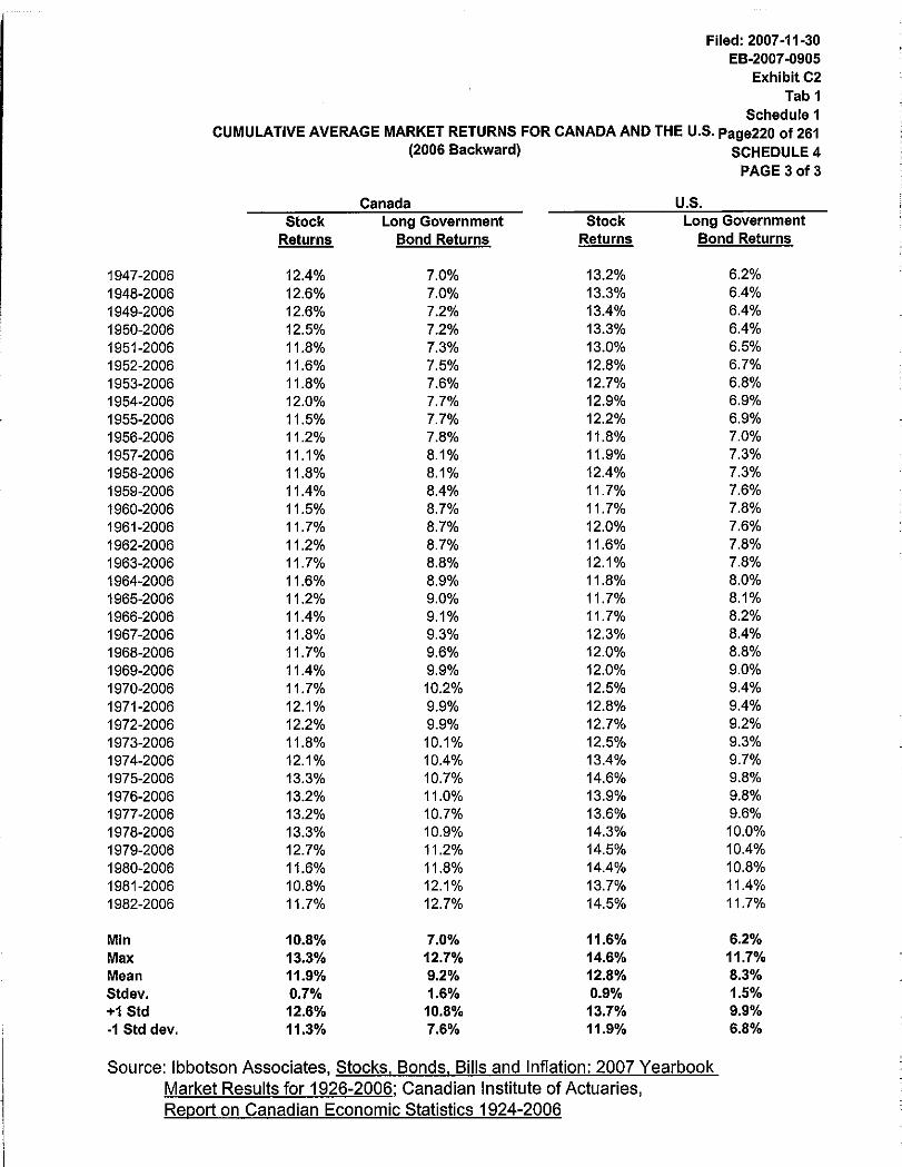
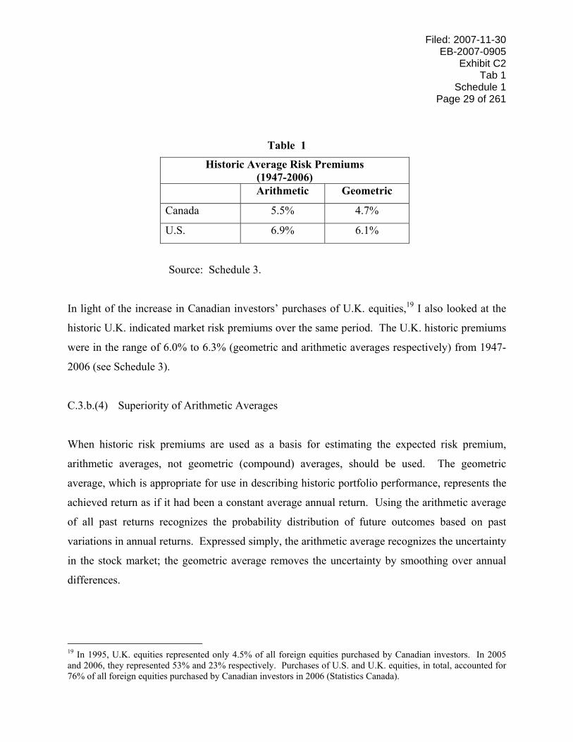
As previously indicated, in arriving at an estimation of the market risk premium, my point of
departure was both Canadian and U.S. historic returns and risk premiums during the post-World
War II period. The average U.S. and Canadian historic risk premiums during that period were as
follows:
18 Key structural economic changes have occurred since the end of World War II, including:
1. The globalization of the North American economies, which has been facilitated by the reduction in trade barriers of which GATT (1947) was a key driver;
2. Demographic changes, specifically suburbanization and the rise of the middle class, which have impacted on the patterns of consumption;
3. Transition from a resource-oriented/manufacturing economy to a service-oriented economy; 4. Technological change, particularly in the areas of telecommunications and computerization, which have
facilitated both market globalization and rising productivity.
Filed: 2007-11-30 EB-2007-0905
Exhibit C2 Tab 1
Schedule 1 Page 29 of 261
Table 1
Historic Average Risk Premiums (1947-2006)
Arithmetic Geometric
Canada 5.5% 4.7%
U.S. 6.9% 6.1%
Source: Schedule 3.
In light of the increase in Canadian investors’ purchases of U.K. equities,19 I also looked at the
historic U.K. indicated market risk premiums over the same period. The U.K. historic premiums
were in the range of 6.0% to 6.3% (geometric and arithmetic averages respectively) from 1947-
2006 (see Schedule 3).
C.3.b.(4) Superiority of Arithmetic Averages
When historic risk premiums are used as a basis for estimating the expected risk premium,
arithmetic averages, not geometric (compound) averages, should be used. The geometric
average, which is appropriate for use in describing historic portfolio performance, represents the
achieved return as if it had been a constant average annual return. Using the arithmetic average
of all past returns recognizes the probability distribution of future outcomes based on past
variations in annual returns. Expressed simply, the arithmetic average recognizes the uncertainty
in the stock market; the geometric average removes the uncertainty by smoothing over annual
differences.
19 In 1995, U.K. equities represented only 4.5% of all foreign equities purchased by Canadian investors. In 2005 and 2006, they represented 53% and 23% respectively. Purchases of U.S. and U.K. equities, in total, accounted for 76% of all foreign equities purchased by Canadian investors in 2006 (Statistics Canada).
Filed: 2007-11-30 EB-2007-0905 Exhibit C2 Tab 1 Schedule 1 Page 30 of 261 C.3.b.(5) Future vs. Historic Risk Premiums
The 1998-2002 equity market “bubble and bust” spawned a number of studies of the equity
market risk premium that have speculated that the U.S. market risk premium will be lower in the
future than in the past. The speculation stems in part from the hypothesis that the magnitude of
the achieved risk premiums is due to an increase in price/earnings (P/E) ratios. That is, the
historic U.S. equity market returns reflect appreciation in the value of stocks in excess of that
supported by the underlying growth in earnings or dividends. The increase in P/E ratios, it has
been argued, reflects a decline in the rate at which investors are discounting future earnings, i.e.,
a lower cost of capital.
I have analyzed the trends in P/E ratios, equity market returns, and bond returns.20 Briefly, that
analysis demonstrates:
♦ The increase in price/earnings ratios experienced during the market bubble of the 1990s
has not resulted in a higher and unsustainable level of equity market returns. The
arithmetic average equity returns in both Canada and the U.S. from 1947-1989 (prior to
the “bubble”) are actually higher than the average returns for the full 1947-2006 period.
♦ An analysis of non-overlapping 10-year average equity returns reveals no upward or
downward trend in equity market returns in Canada or the U.S. over the post World War
II period.
♦ The observed decline in the experienced risk premium is due to the unsustainable
increase in bond returns, not a decline in equity returns. The observed historic bond
returns are significantly higher than a reasonable estimate of future bond returns (that is,
forecast yields of long Canada bond yields).
Given the absence of any upward or downward trend in the historic equity market returns, a
reasonable expected value of the future equity market return is a range of 11.5-12.25%, based on 20 See Appendix C for further discussion.
Filed: 2007-11-30 EB-2007-0905
Exhibit C2 Tab 1
Schedule 1 Page 31 of 261
both the Canadian and U.S. equity market returns (see Appendix C). Based on both the near-
term and the longer-term forecasts for long Canada bond yields of 5.0% (2008) and 5.25%
(average of 2009-2017),21 and an expected equity market return of 11.5-12.5%, the indicated
Canadian equity market risk premium would be in the range of 6.5-7.25%.22
C.3.b.(6) Estimate of Equity Market Risk Premium
Based on the analysis of the historic risk premiums, primarily in Canada and the U.S., with focus
on the arithmetic averages, and with consideration given to trends in the equity and government
bond markets in both countries, a reasonable estimate of the expected value of the equity market
risk premium at the forecast levels of long-term government bond yields is approximately 6.5%.
This estimate explicitly recognizes the expected value of the equity market return developed
from historic values in conjunction with the current and forecast low levels of interest rates.
C.3.c. Relative Risk Adjustment
C.3.c.(1) Total Market Risk
The market risk premium result needs to be adjusted to recognize the relatively lower risk of
utilities. The relative risk adjustment that is applicable to a benchmark Canadian utility is
approximately 0.65-0.70, based on total risk as measured by standard deviations of market
returns and adjusted betas.
My analysis of the relative risk adjustment starts with a recognition that investors are not
perfectly diversified, do look at the risks of individual investments, and require compensation for
assuming company-specific or investment-specific risk. It also recognizes that, while investors
21 Consensus Economics, Consensus Forecasts, April 2007 anticipates the 10-year Canada bond yield to average approximately 5.1% from 2009 to 2017. Adding a spread of approximately 10 (as of August 2007) to 30 (historic average) basis points to the 5.1% forecast results in a 30-year Canada bond yield forecast of close to 5.25%. 22 11.5% - 5.0% = 6.5% 12.5% - 5.25% = 7.25%
Filed: 2007-11-30 EB-2007-0905 Exhibit C2 Tab 1 Schedule 1 Page 32 of 261 can diversify their portfolios, the stand-alone utility to which the allowed return is applied
cannot. Thus, a risk measurement that reflects those considerations is relevant for estimating the
utility equity risk premium. These considerations support focusing on total market risk, as well
as on beta, which is intended to measure solely non-diversifiable risk. The drawbacks of beta as
the sole measure of risk, as well as the absence of an observable relationship between “raw”
betas23 and the achieved market returns on equity in the Canadian market, provide further
support for reliance on other measures of risk to estimate the required equity return (see
Appendix C).
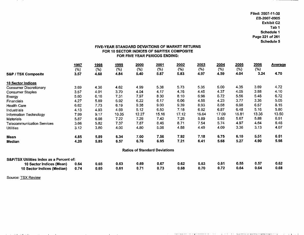
The standard deviation of market returns is the principal measurement of total market risk. To
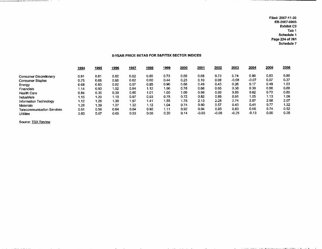
compare the relative total risk of Canadian utilities, I calculated the monthly standard deviations
of total market returns for each of the 10 major Sectors of the S&P/TSX Index, over recent five-
year periods ending 1997 through 2006 (Schedule 5).
To translate the standard deviation of market returns into a relative risk adjustment, utility
standard deviations must be related to those of the overall market. The relative market volatility
of Canadian utility stocks was measured by comparing the standard deviations of the Utilities
Index to the simple mean and median of the standard deviations of the 10 Sectors. Schedule 5
shows the ratios of the standard deviations of the Utilities Index to those of the 10 S&P/TSX
Sectors. The ratio of the standard deviation of the Utilities Index to the mean and median
standard deviations of the 10 major Sector Indices suggests a relative risk adjustment for a
benchmark Canadian utility in the range of 0.55-0.74, with a central tendency of approximately
0.65-0.70.
23 The “raw” beta refers to the simple regression between the monthly percentage changes in the price of a utility or utility index and the corresponding percentage change in the price of the equity market index (the S&P/TSX Composite).
Filed: 2007-11-30 EB-2007-0905
Exhibit C2 Tab 1
Schedule 1 Page 33 of 261
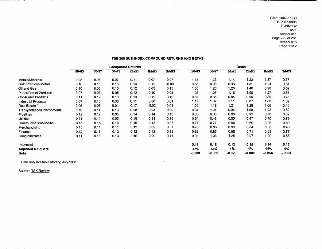
C.3.c.(2) Historic Raw Betas
Since beta remains the risk measure that underpins the application of the Capital Asset Pricing
Model (CAPM) (of which the risk-adjusted equity market risk premium test is a variant), I also
considered betas in arriving at the estimated relative risk adjustment for a benchmark utility.
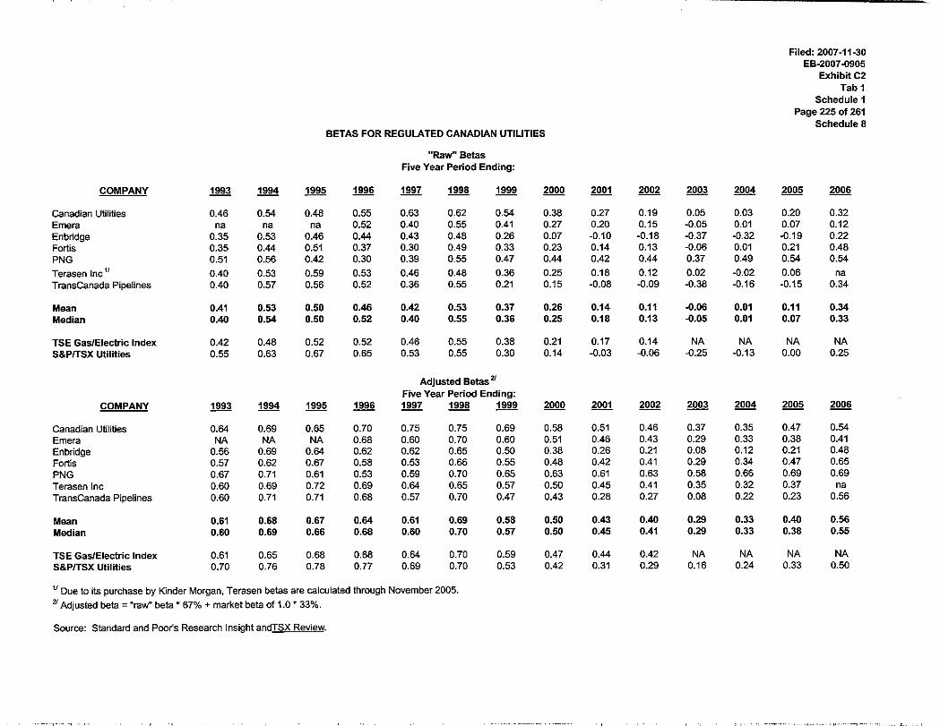
Schedule 8 summarizes “raw” betas for individual publicly-traded Canadian regulated electric
and gas companies, the TSE Gas/Electric Index, and the S&P/TSX Utilities Sector over five-year
periods ending 1993 through 2006.24
As Schedule 8 indicates, there was a significant decline in calculated “raw” betas between 1993-
1998 and 1999-2005 (from approximately 0.50-0.60 to 0.0 and slightly negative) followed by an
increase in 2006 to the 0.25 to 0.35 range. The observed levels of “raw” utility betas in 1999-
2006 can be traced to three factors: (1) the technology sector bubble and subsequent bust; (2) the
dominance in the TSE 300 of two firms during the early part of the “bubble and bust” period,
Nortel Networks and BCE; (3) the negative impact of rising interest rates on utility stock prices
while the equity market composite is otherwise increasing (e.g., during the “bubble” of 1999 and
early 2000 and during the first half of 2006).
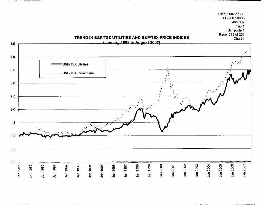
Chart 1 in the Statistical Exhibit graphically demonstrates the “decoupling” between utility
stocks and the S&P/TSX Composite between 1999 and mid-2002 period, when the equity market
“bubble and bust” was most prevalent. As a result, the disparate movements in utility equities
relative to the S&P/TSX Composite during this period produced lower measured utility betas.
Chart 1 also shows that, beginning in mid-2002, the equity market composite and the utility
equities began to once again exhibit a correlation that, graphically, resembled more closely the 24 The S&P/TSX Utilities Sector was created in 2002 (with historic data calculated from year-end 1987), when the TSE 300 was revamped to create the S&P/TSX Composite. The Utilities Sector was essentially an amalgamation of the former TSE 300 Gas/Electric and Pipeline sub-indices. In May 2004, the pipelines were moved to the Energy Sector, and no longer comprise a separate sub-index.

Filed: 2007-11-30 EB-2007-0905 Exhibit C2 Tab 1 Schedule 1 Page 34 of 261 typical relationship observed prior to the market “bubble and bust”. Utility betas calculated over
recent periods that largely eliminate the “bubble and bust” period are higher than those that
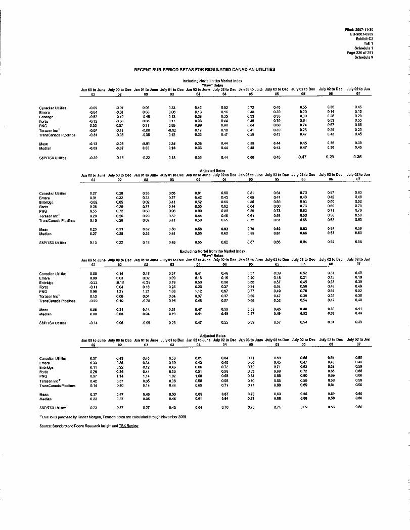
include data from this period. However, rising interest rates in early 2006 and the resulting
negative impact on utility stock prices has again reduced the calculated “raw” utility betas
(Schedule 9).25
The decoupling between utility shares and the rest of the market during both the technology
“bubble and bust” and the first half of 2006 should not be interpreted as a change in the relative
riskiness of utility shares,26 but rather as an indication of the weakness of beta as the sole
measure of the relative equity return requirement, particularly within the Canadian equity market
context.27
25 Calculated with Nortel excluded from the Composite to remove any lingering effects on the behaviour of the Composite. 26 Schedule 7 shows that utilities were not the only companies whose betas were negatively impacted by the speculative bubble and subsequent market decline. To illustrate, the 60-month beta ending 1997 of the Consumer Staples Sector was 0.62; the corresponding betas ending 2003 and 2004 were -0.08 and -0.07 respectively. In contrast, over the same periods, the beta of the Information Technology Sector rose from 1.57 to 2.87. 27 For example, with the rise in energy stock prices the 60-month betas for the S&P/TSX Energy Sector rose from 0.17 in 2004, to 0.48 in 2005 to over 1.0 in 2006 suggesting a five-fold increase in risk for these companies. (Schedule 7)
Filed: 2007-11-30 EB-2007-0905
Exhibit C2 Tab 1
Schedule 1 Page 35 of 261
C.3.c.(3) Impact of Interest Sensitivity on Relative Risk
Utilities are interest-sensitive stocks and thus tend to move with interest rates, which frequently
move counter to the equity market. Consequently, utility equity price movements are correlated
not only with the stock market, but also with movements in the bond market. Thus, the interest-
sensitivity of utility shares is not fully captured in the calculated “raw” betas, which simply
measure the covariability between a stock and the equity market composite.28 An analysis of the
relative historic sensitivity of utility shares to both interest rates and the equity market indicates a
relative risk adjustment of close to 80% (see Appendix C).
C.3.c.(4) Use of Adjusted Beta
The deficiencies in “raw” beta can be mitigated by using adjusted betas. Adjusting betas entails
moving betas above and below the market mean of 1.0 toward the market mean. The adjustment
that is used by the major commercial suppliers of betas uses a formula that gives approximately
two-thirds weight to the stock’s own beta and one-third weight to the market mean beta of 1.0.29
Use of adjusted betas implicitly recognizes that “raw” utility betas do not adequately explain
utility returns. For example, as illustrated above, “raw” betas do not capture utilities’ interest
rate sensitivity. Further, the objective of the relative risk adjustment is to predict the investors’
required return. Since utility returns have consistently been higher than what raw betas would
indicate, adjusted betas are better predictors of utility returns than “raw” betas.30
28 In theory, the beta should be measured against the entire “capital market” including short-term debt securities, bonds, real estate, etc. In practice, it is measured using the equity market only. 29 Value Line, Bloomberg and Merrill Lynch, major sources of financial information for investors, all publish adjusted betas. Their formulas for adjusting the calculated raw betas are slightly different, but all give approximately two-thirds weight to the “raw” beta of the specific stock and one-third weight to the market beta of 1.0. 30 More generally, a number of empirical studies on CAPM have shown that the return requirement is higher (lower) for a low (high) beta stock than the CAPM would predict.
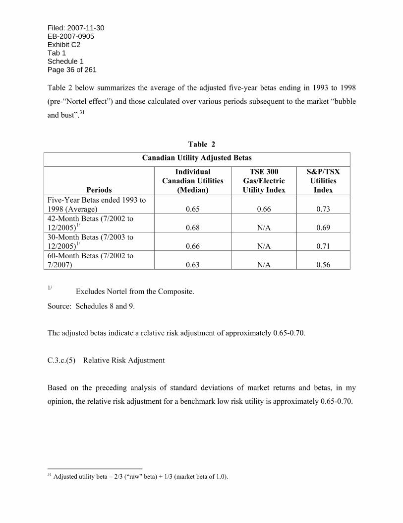
Filed: 2007-11-30 EB-2007-0905 Exhibit C2 Tab 1 Schedule 1 Page 36 of 261 Table 2 below summarizes the average of the adjusted five-year betas ending in 1993 to 1998
(pre-“Nortel effect”) and those calculated over various periods subsequent to the market “bubble
and bust”.31
Table 2
Canadian Utility Adjusted Betas
Periods
Individual Canadian Utilities
(Median)
TSE 300 Gas/Electric Utility Index
S&P/TSX Utilities Index
Five-Year Betas ended 1993 to 1998 (Average)
0.65
0.66
0.73
42-Month Betas (7/2002 to 12/2005)1/
0.68
N/A
0.69
30-Month Betas (7/2003 to 12/2005)1/
0.66
N/A
0.71
60-Month Betas (7/2002 to 7/2007)
0.63
N/A
0.56
1/ Excludes Nortel from the Composite.
Source: Schedules 8 and 9.
The adjusted betas indicate a relative risk adjustment of approximately 0.65-0.70.
C.3.c.(5) Relative Risk Adjustment
Based on the preceding analysis of standard deviations of market returns and betas, in my
opinion, the relative risk adjustment for a benchmark low risk utility is approximately 0.65-0.70.
31 Adjusted utility beta = 2/3 (“raw” beta) + 1/3 (market beta of 1.0).
Filed: 2007-11-30 EB-2007-0905
Exhibit C2 Tab 1
Schedule 1 Page 37 of 261
C.3.d. Benchmark Utility Equity Risk Premium
I previously estimated the equity market risk premium at the long Canada yield of 5.0%, at
approximately 6.5%. At an equity market risk premium of 6.5% and a relative risk adjustment of
0.65-0.70, the indicated benchmark utility equity risk premium is approximately 4.25-4.50%.32
C.4. Utility-Specific Equity Risk Premium Analysis
The risk-adjusted equity market risk premium test (discussed above) estimates the required
utility equity risk premium indirectly. That is, it estimates an equity risk premium for the equity
market as a whole, and then adjusts it for the relative risk of a benchmark utility. The following
analyses estimate the equity risk premium for a benchmark utility directly, by analyzing utility
equity return data. The analyses below focus on both long-term historic utility equity risk
premiums and an equity risk-premium test derived from forward-looking monthly estimates of
the required utility equity return.
The following two sections provide the results of that analysis.
C.4.a. Historic Utility Equity Risk Premiums
The historic experienced returns for utilities provide an additional perspective on a reasonable
expectation for the forward-looking utility equity risk premium. Reliance on achieved equity
risk premiums for utilities as an indicator of what investors expect for the future is based on the
proposition that over the longer term, investors’ expectations and experience converge. The
more stable an industry, the more likely it is that this convergence will occur.
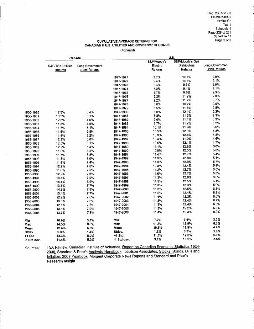
Over the longer-term (1956-2006),33 achieved utility equity risk premiums were 4.1-4.8% for
Canadian electric and gas utilities, based on geometric and arithmetic average returns 32 (0.65-0.70) x 6.5% = 4.25-4.50%

Filed: 2007-11-30 EB-2007-0905 Exhibit C2 Tab 1 Schedule 1 Page 38 of 261 respectively.34 For U.S. electric utilities, the corresponding geometric and arithmetic average
historic equity risk premiums were approximately 4.5-5.2% over the entire post-World War II
period (1947-2006). The corresponding risk premiums for U.S. gas utilities were 5.5-6.2%
(Schedule 10).
Similar to the risk premiums for the market composite, the magnitude of achieved utility risk
premiums is a function of both the equity returns and the bond returns, as summarized for
Canadian utilities in the table below.
Table 3
Canadian Utility Risk Premiums 1956-2006 Average Utility Equity
Returns Bond Returns Achieved Risk
Premiums Arithmetic 12.6% 7.8% 4.8%
Geometric 11.5% 7.4% 4.1%
Source: Schedule 10.
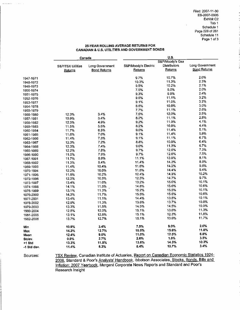
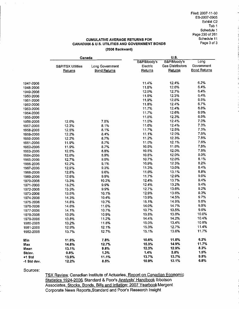
An analysis of the underlying data indicates there has been no upward or downward trend in the
utility equity returns (Schedule 11); the utility returns in both the U.S. and Canada have clustered
in the approximate range of 11.0-12.0%. However, as noted in Appendix C, the bond returns
have risen over the fifty-year period to a level that cannot persist, given the low level of interest
rates. The low level of interest rates limits further capital gains on bonds (which have given rise
to the high observed bond returns in recent years). The best estimate of the expected bond return
is the forecast yields on long Canada bond yields, which are in the range of 5.0-5.25%, based on
33 The longest period for which Canadian utility data are available from the TSE. 34 Based on the Gas/Electric Index of the TSE 300 (from 1956 to 1987) and on the S&P/TSX Utilities Index from 1988-2006.

Filed: 2007-11-30 EB-2007-0905
Exhibit C2 Tab 1
Schedule 1 Page 39 of 261
both near-term and long-term forecasts. When that yield is compared to a utility equity return of
11.0-12.0%, the indicated equity risk premium is approximately 6.0-6.75%.35
Focusing on the arithmetic average risk premiums, and recognizing that historic bond returns
overstate the expected bond return, the experience of Canadian and U.S. utilities supports an
expected equity risk premium estimate for a benchmark Canadian utility in the approximate
range of 5.0-5.5%.
C.4.b. DCF-Based Equity Risk Premium Test
A forward-looking equity risk premium test was also performed, using the discounted cash flow
model (DCF) to estimate expected utility returns over time. Monthly cost of equity estimates
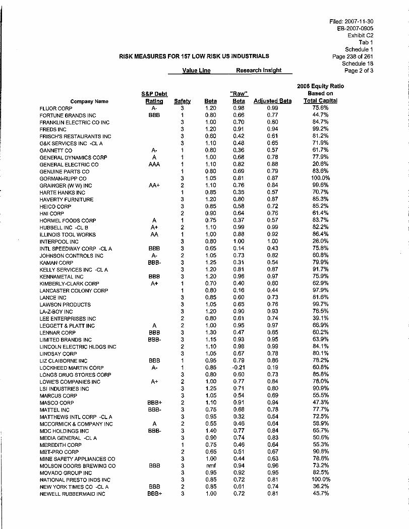
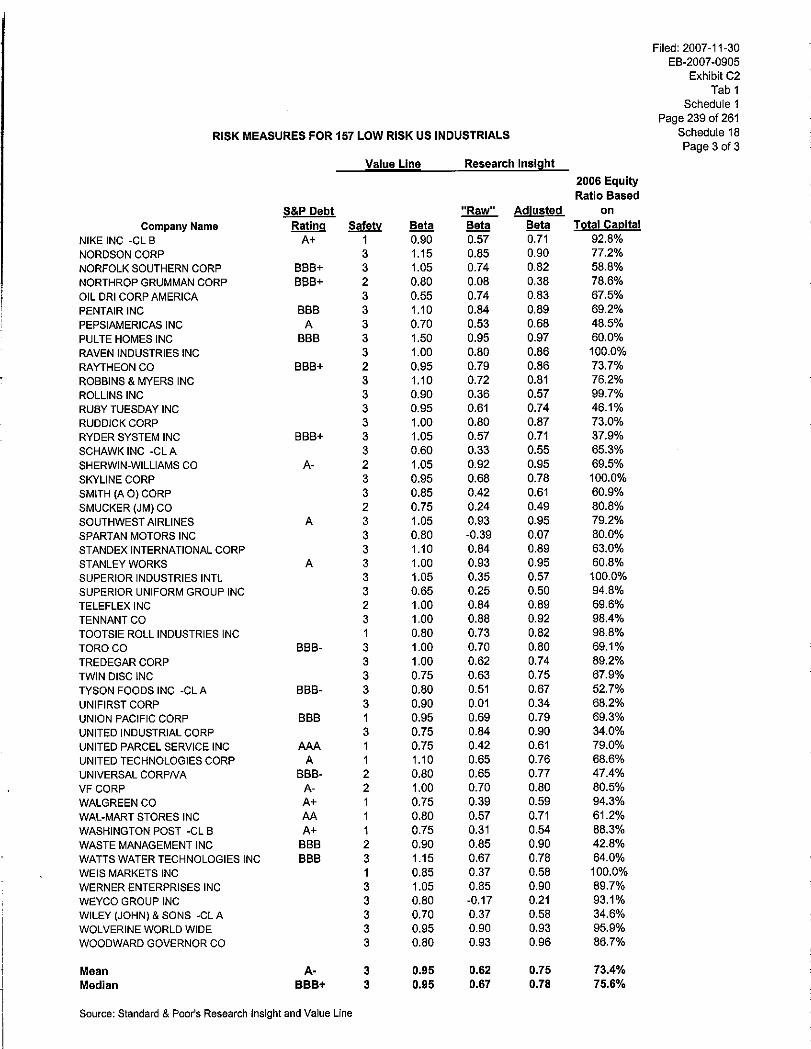
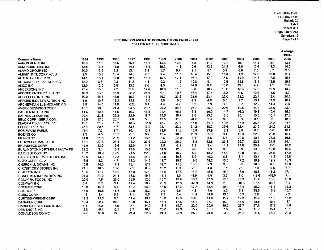
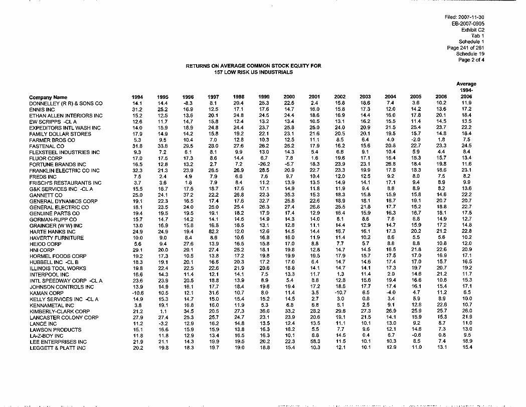
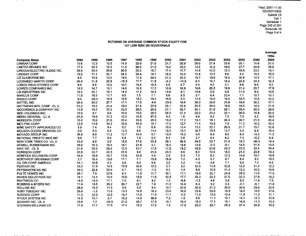
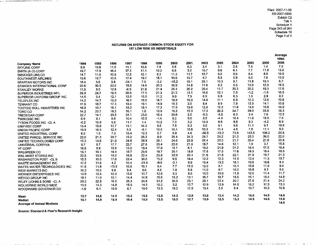
were constructed for the period 1993-2007 (2nd Qtr)36 using the DCF model and a sample of low
risk U.S. electric and gas utilities as a proxy for a benchmark Canadian utility.37 The reasons for
choosing U.S. utilities are as follows:
First, there are an insufficient number of forward-looking estimates of long-term growth rates for
Canadian utilities that would permit the creation of a consistent series of DCF costs of equity and
corresponding risk premiums from Canadian data. A consensus estimate of investors’ growth
expectations is key to the application of the discounted cash flow model. The availability of a
consensus of analysts’ forecasts means that the resulting growth estimate reflects the market
view.
35 11.0% - 5.0% = 6.0% 12.0% - 5.25% = 6.75% 36 The period 1993-2007 (2nd Qtr) encompasses a full business cycle. It also represents the period of Open Access (implemented via FERC Order 636) for gas distributors which make up close to 50% of the benchmark low risk utility sample. 37 The selection criteria for the proxy utilities and the construction of the DCF estimates are described in Appendix D.
Filed: 2007-11-30 EB-2007-0905 Exhibit C2 Tab 1 Schedule 1 Page 40 of 261 Second, U.S. and Canadian utilities are reasonable proxies for one another, particularly in
today’s global capital market. Although there may be company-specific differences in business
and financial risk, the impact of those differences is minimized by selecting only relatively pure-
play U.S. utilities with similar debt ratings to the typical Canadian utility. The selected U.S.
utilities are of relatively low business risk; the sample, which is limited to utilities with debt
ratings in the A category, is of similar total risk to a benchmark Canadian utility.
The DCF costs of equity were estimated as the sum of the consensus of analysts’ forecasts of
long-term normalized earnings growth,38 plus the expected dividend yield. The equity risk
premium is equal to the difference between the average DCF cost of equity for the sample and
the corresponding 30-year Treasury yield for the period.
For the sample of U.S. utilities, the DCF-based risk premium test indicates an average risk
premium over the 1993-2007 (2nd Qtr) period of 4.0% (Schedule 12); the corresponding average
long-term government bond yield was 5.8%, approximately 75 basis points higher than the test
period forecast yield on long Canada bond yields of 5.0%. I also looked at the average risk
premium over the period 1998-2007 (2nd Qtr), representing the period subsequent to open access
for electric utilities in the U.S.39 The average risk premium over that period was 4.5%, with a
corresponding government bond yield of 5.3%.
The data suggest that there has been an inverse relationship between the risk-free rate (as proxied
by the long-term government bond yield) and utility equity risk premiums. To test the
relationship between interest rates and risk premiums, a simple regression analysis between the
monthly 30-year Treasury yields and the corresponding equity risk premiums over the entire
38 The consensus forecasts are obtained from I/B/E/S, a leading provider of earnings expectations data. The data are collected from over 7,000 analysts at over 1,000 institutions worldwide, and cover companies in more than 60 countries. 39 Open access for electric utilities was implemented via FERC Order 888 in 1997.
Filed: 2007-11-30 EB-2007-0905
Exhibit C2 Tab 1
Schedule 1 Page 41 of 261
1993-2007 (2nd Qtr) period was conducted.40 At the test year forecast 30-year government bond
yield of 5.0%, the indicated utility equity risk premium is approximately 4.5%.
The magnitude of the spread between corporate bond yields and government bond yields is
frequently used as a proxy for changes in investors’ perception of risk.41 Thus, I also tested the
relationship between the spreads between long-term utility and government bond yields in
conjunction with the change in the yield on long-term government bond yields.
To estimate this relationship, I performed a regression analysis over the 1993-2007 (2nd Qtr)
period using the utility risk premium42 as the dependent variable, with the corresponding long-
term government bond yield and spread between long-term A-rated utility43 and government
bond yields as the two independent variables.44 The analysis indicated that, while the utility risk
premium has been negatively related to the level of government bond yields, it has been
positively related to the spread between utility bond yields and government bond yields. The
spread between long-term Canadian A-rated utility bonds and 30-year Canada bond yields was
approximately 130 basis points at the end of August 2007, compared to the average Moody’s A-
rated utility/30-year Treasury spread of 139 basis points over the entire 1993-2007 (2rd Qtr)
period. Using a forecast long Canada yield of 5.0% and an A-rated utility bond/long Canada
spread of 130 basis points, the indicated utility risk premium is 4.3%.
40 Equity Risk premium = 7.56 – 0.606 (30-Year Treasury yield) t-statistic = -11.0 R2 = 41% 41 Or, alternatively, willingness to take risks. 42 Measured, as in the prior analysis, as the DCF cost of equity minus the long-term government bond yield. 43 Based on Moody’s long-term A- rated utility bond index. 44 Utility Risk Premium = 4.9 - 0.41 TY + 1.12 Spread Where, TY = 30-year Treasury Yield Spread = Spread between A-rated Utility Bond Yields and 30-year Treasury Yields R2 = 80% t-statistics: Long term bond yield = -12.2 Utility/government bond yield spread = 18.2
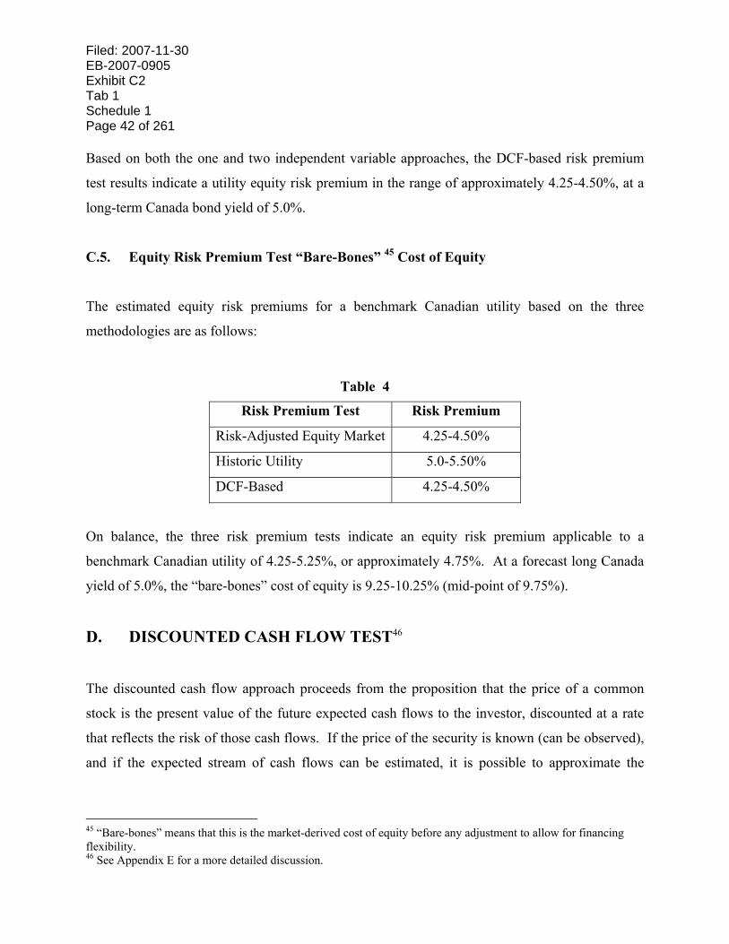
Filed: 2007-11-30 EB-2007-0905 Exhibit C2 Tab 1 Schedule 1 Page 42 of 261 Based on both the one and two independent variable approaches, the DCF-based risk premium
test results indicate a utility equity risk premium in the range of approximately 4.25-4.50%, at a
long-term Canada bond yield of 5.0%.
C.5. Equity Risk Premium Test “Bare-Bones” 45 Cost of Equity
The estimated equity risk premiums for a benchmark Canadian utility based on the three
methodologies are as follows:
Table 4
Risk Premium Test Risk Premium
Risk-Adjusted Equity Market 4.25-4.50%
Historic Utility 5.0-5.50%
DCF-Based 4.25-4.50%
On balance, the three risk premium tests indicate an equity risk premium applicable to a
benchmark Canadian utility of 4.25-5.25%, or approximately 4.75%. At a forecast long Canada
yield of 5.0%, the “bare-bones” cost of equity is 9.25-10.25% (mid-point of 9.75%).
D. DISCOUNTED CASH FLOW TEST46
The discounted cash flow approach proceeds from the proposition that the price of a common
stock is the present value of the future expected cash flows to the investor, discounted at a rate
that reflects the risk of those cash flows. If the price of the security is known (can be observed),
and if the expected stream of cash flows can be estimated, it is possible to approximate the
45 “Bare-bones” means that this is the market-derived cost of equity before any adjustment to allow for financing flexibility. 46 See Appendix E for a more detailed discussion.
Filed: 2007-11-30 EB-2007-0905
Exhibit C2 Tab 1
Schedule 1 Page 43 of 261
investor’s required return (or capitalization rate) as the rate that equates the price of the stock to
the discounted value of future cash flows.
Although the DCF test, like the equity risk premium test, has flaws, it has one distinct advantage
over risk premium estimates, particularly those made using the CAPM. It allows the analyst to
directly estimate the utility cost of equity. In contrast, the CAPM indirectly estimates the cost of
equity. The DCF model provides a widely used alternative to the CAPM; it is the principal
model utilized by U.S. regulators.
There are multiple versions of the discounted cash flow model available to estimate the
investor’s required return. An analyst can employ a constant growth model or a multiple period
model to estimate the cost of equity. The constant growth model rests on the assumption that
investors expect cash flows to grow at a constant rate throughout the life of the stock. Similarly,
a multiple period model rests on the assumption that growth rates will change over the life of the
stock. In determining the DCF cost of equity for a benchmark utility, I utilized both a constant
growth and a two-stage model.47 In both cases, the discounted cash flow test was applied to a
sample of low risk U.S. “pure-play” electric and gas distributors that are intended to serve as a
proxy for a benchmark Canadian utility.48
The growth component of the DCF model is an estimate of what investors expect over the
longer-term. For a regulated utility, whose growth prospects are tied to allowed returns, the
estimate of growth expectations is subject to circularity because the analyst is, in some measure,
attempting to project what returns the regulator will allow, and the extent to which the utilities
will exceed or fall short of those returns. To mitigate that circularity, it is important to rely on a
sample of proxies, rather than the subject company. (When the subject company does not have
traded shares, a sample of proxies is required.)
47 The two-stage model is a form of multiple period model; please see Appendix E for discussion of the DCF models used; the criteria for the low risk U.S. utility sample selection are described in Appendix D. 48 Reliance on U.S. utilities was explained in the discussion of the DCF-based equity risk premium test in Chapter III.C.4.b.
Filed: 2007-11-30 EB-2007-0905 Exhibit C2 Tab 1 Schedule 1 Page 44 of 261
Further, to the extent feasible, one should rely on estimates of longer-term growth readily
available to investors, rather than superimpose on the analysis one’s own view of what growth
should be. Thus, in applying the DCF test, I relied solely on published forecast growth rates that
are readily available to investors. The constant growth model uses the consensus of analysts’
earnings growth rate forecasts as the proxy for investors’ long-term growth expectations. The
two-stage model is based on the premise that investors expect the growth rate for the utilities to
be equal to the analysts’ forecasts (which are five year projections) for the first five years, but, in
the longer-term (from year 6 onward) to migrate to the expected long-run rate of nominal growth
in the economy.
The results of the constant growth and two-stage DCF models indicate a required “bare-bones”
return on equity of approximately 9.25-9.5% (Appendix E and Schedules 14 and 15). It is
important to recognize that the 9.25-9.5% DCF cost represents the return investors expect to earn
on the current market value of their utility common equity investments. It is not, however, the
return that investors expect the utilities to earn on the book value of their common equity. Value
Line, which publishes its projections of utility ROEs quarterly, anticipates that the return on
average common equity for the sample of low risk U.S. utilities over the period 2010-2012 will
be approximately 11.2-12.0% (Schedule 13).
E. ALLOWANCE FOR FINANCING FLEXIBILITY49
The financing flexibility allowance is an integral part of the cost of capital as well as a required
element of the concept of a fair return. The allowance is intended to cover three distinct aspects:
(1) flotation costs, comprising financing and market pressure costs arising at the time of the sale
of new equity; (2) a margin, or cushion, for unanticipated capital market conditions; and (3) a
recognition of the "fairness" principle.
49 See Appendix G for a more complete discussion.
Filed: 2007-11-30 EB-2007-0905
Exhibit C2 Tab 1
Schedule 1 Page 45 of 261
In the absence of an adjustment for financial flexibility, the application of a “bare-bones” cost of
equity to the book value of equity, if earned, in theory, limits the market value of equity to its
book value. The fairness principle recognizes the ability of competitive firms to maintain the
real value of their assets in excess of book value and thus would not preclude utilities from
achieving a degree of financial integrity that would be anticipated under competition. The
market/book ratio of the S&P/TSX Composite has averaged 2.1 times over the past business
cycle (1994-2006); the corresponding average market/book ratio of the S&P 500 has been 3.4
times.
At a minimum, the financing flexibility allowance should be adequate to allow a utility to
maintain its market value, notionally, at a slight premium to book value, i.e., in the range of 1.05-
1.10. At this level, a utility would be able to recover actual financing costs, as well as be in a
position to raise new equity (under most market conditions) without impairing its financial
integrity. A financing flexibility allowance adequate to maintain a market/book in the range of
1.05-1.10 is approximately 50 basis points.50 As this financing flexibility adjustment is minimal,
it does not fully address the comparable return standard.
The concept of a financing flexibility or flotation cost allowance has been accepted by most
Canadian regulators. As a government-owned utility, OPG has not raised equity capital in the
public equity markets; therefore it does not incur out-of-pocket equity financing and market
pressure costs. However, both the cushion, or safety margin, for unanticipated capital market
conditions and the fairness element are integral components of the cost of equity and a fair return
on the book value of equity. Both should be recognized in the allowed return on equity for a
regulated utility, irrespective of ownership. The Board has implicitly recognized this principle in
the past (e.g., in its Transitional Rate Order (Distribution) for Hydro One, RP-1998-0001), by
setting returns for the government-owned utilities that are comparable to those allowed for
investor-owned utilities.
50 Based on the DCF model; see Appendix G for calculation.
Filed: 2007-11-30 EB-2007-0905 Exhibit C2 Tab 1 Schedule 1 Page 46 of 261 The addition of an allowance for financing flexibility of 50 basis points to the “bare-bones”
return on equity estimate of 9.25-10.25% derived from both the DCF and equity risk premium
tests respectively, results in an estimate of the fair return on equity of 9.75%-10.75%.
F. COMPARABLE EARNINGS TEST
The comparable earnings test provides a measure of the fair return based on the concept of
opportunity cost. Specifically, the test arises from the notion that capital should not be
committed to a venture unless it can earn a return commensurate with that available
prospectively in alternative ventures of comparable risk. Since regulation is a surrogate for
competition, the opportunity cost principle entails permitting utilities the opportunity to earn a
return commensurate with the levels achievable by competitive firms facing similar risk. The
comparable earnings test, which measures returns in relation to book value, is the only test that
can be directly applied to the equity component of an original cost rate base without an
adjustment to correct for the discrepancy between book values and current market values.
Neither the equity risk premium results nor the DCF results, if left without adjustment,
recognizes the discrepancy. The 50 basis point financing flexibility adjustment only minimally
addresses the discrepancy.
The comparable earnings test is an implementation of the comparable earnings standard, as
distinguished from the cost of attracting capital standard. The comparable earnings standard
recognizes that utility costs are measured in vintaged dollars and that rates are based on
accounting costs, not economic costs. In contrast, the cost of attracting capital standard relies on
costs expressed in dollars of current purchasing power, i.e., a market-related cost of capital. In
the absence of experienced inflation, the two concepts would be quite similar, but the impact of
inflation has rendered them dissimilar and distinct.
The concept that regulation is a surrogate for competition may be interpreted to mean that the
combination of an original cost rate base and a fair return should result in a value to investors
Filed: 2007-11-30 EB-2007-0905
Exhibit C2 Tab 1
Schedule 1 Page 47 of 261
commensurate with that of competitive ventures of similar risk. The fact that an original cost
rate base provides a starting point for the application of a fair return does not mean that the
original cost of the assets is a measure of their fair value. The concept that regulation is a
surrogate for competition implies that the regulatory application of a fair return to an original
cost rate base should result in a value to investors commensurate with that of similar risk
competitive ventures. The comparable earnings standard, as well as the principle of fairness,
suggests that, if competitive industrial firms facing a level of total risk similar to utilities are able
to maintain the value of their assets considerably above book value, the return allowed to utilities
should not seek to maintain the value of utility assets at book value. It is critical that the
regulator recognize the comparable earnings standard when setting a just and reasonable return.
The comparable earnings test remains the only test that explicitly recognizes that, in the North
American regulatory framework, the return is applied to an original cost (book value) rate base.
The persistence of moderate inflation continues to create systematic deviations between book
and market values. Application of a market-derived cost of capital to book value ignores that
distinction. To illustrate, if the market value of an investment is $15 and the required return is
10%, the return, in dollars, expected by investors is $1.50. However, regulatory convention
applies the market-derived return to the book value of the investment. If the book value of the
investment is $10.00, application of a 10% return to the book value will result in a return, in
dollars, of only $1.00. The application of the results of the cost of attracting capital tests, i.e.,
equity risk premium and discounted cash flow to the book value of equity, unless adjusted, do
not make any allowance for the discrepancy between the return on market value and the
corresponding fair return on book value.51 The comparable earnings test, however, does. It
applies “apples to apples”, i.e., a book value-measured return is applied to a book value-
measured equity investment.
51 As previously noted, the 50 basis point financing flexibility adjustment is only a minimal recognition of the discrepancy.
Filed: 2007-11-30 EB-2007-0905 Exhibit C2 Tab 1 Schedule 1 Page 48 of 261 The principal issues in the application of the comparable earnings test are:52
♦ The selection of a sample of industrials of reasonably comparable risk to a benchmark
Canadian utility.
♦ The selection of an appropriate time period over which returns are to be measured in
order to estimate prospective returns.
♦ The need for any adjustment to the "raw" comparable earnings results if the selected
industrials are not of precisely equivalent risk to the benchmark utility.
♦ The need for a downward adjustment for the industrials’ market/book ratios.
The application of the comparable earnings test first requires the selection of one or more
samples of industrials of reasonably comparable risk to a benchmark Canadian utility. The
selection should conform to investor perceptions of the risk characteristics of utilities, which are
generally characterized by relative stability of earnings, dividends and market prices. These
were the principal criteria for the selection of samples of industrial companies (from consumer-
oriented industries). The criteria for selecting comparable unregulated low risk companies
include industry, size, dividend history, stock and bond ratings and betas (See Appendix F).
Since the universe of Canadian industrial companies is sufficiently large to produce a
representative sample of sufficient size, the focus of the comparable earnings analysis was on
Canadian firms. However, a sample of U.S. companies was also used as a check on the
reasonableness of the Canadian sample results. The application of the selection criteria to the
Canadian universe produced a sample of 20 companies.
Next, since industrials’ returns on equity tend to be cyclical, the selection of an appropriate
period for measuring industrial returns must be determined. The period selected should
encompass an entire business cycle, covering years of both expansion and decline. That cycle
should be representative of a future normal cycle, e.g., the historic and forecast cycles should be 52 Full discussion in Appendix F.
Filed: 2007-11-30 EB-2007-0905
Exhibit C2 Tab 1
Schedule 1 Page 49 of 261
similar in terms of inflation and real economic growth.53 The period 1994-2006 provides a
reasonable proxy for a future business cycle, as the experienced rates of inflation and economic
growth are reasonably similar to the rates projected by economists over the next business cycle.
The experienced returns on equity of the sample of 20 Canadian low risk industrial companies
over this period were in the approximate range of 12.75-13.25% (see Appendix F and Schedule
17).
The next step is to assess whether or not there is a need to adjust the “raw” comparable earnings
results to reflect the differential risk of a benchmark Canadian utility relative to the selected
industrials. The comparative risk data (including betas and stock and bond ratings) indicate, on
balance, the Canadian industrials are of modestly higher risk than a benchmark utility. To
recognize the industrials’ higher risk, the comparable earnings test results require a downward
adjustment to a range of 12.25-12.75% (mid-point of 12.50%).
Since the Canadian sample is relatively small, in large part a function of the size and make-up of
the Canadian equity market, as noted above, I also selected a sample of low risk U.S. industrials
to serve as a check on the reasonableness of the Canadian results. The selection criteria were
virtually identical to those used for the Canadian industrial sample. The greater breadth of the
U.S. market allowed the selection of a sample of 157 companies in the same stable industries
used to select the Canadian industrials. The experienced returns of the U.S. industrials were in
the range of 13.5-14.5% (see Schedule 19). The comparative risk data indicate that the U.S.
industrials are of relatively similar risk to the Canadian industrials (see Schedule 18), and thus of
slightly higher risk than a benchmark Canadian utility. When used as a check against the
Canadian firms, the returns of the significantly larger U.S. sample of industrials underscore the
reasonableness of the comparable earnings results for the sample of Canadian industrials.
53 Returns on equity during earlier periods may not be comparable as the economic fundamentals that impact achievable returns (e.g., inflation) were not comparable.
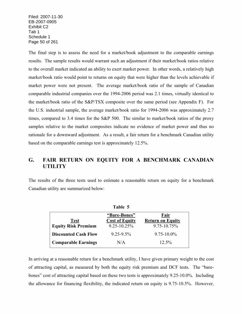
Filed: 2007-11-30 EB-2007-0905 Exhibit C2 Tab 1 Schedule 1 Page 50 of 261 The final step is to assess the need for a market/book adjustment to the comparable earnings
results. The sample results would warrant such an adjustment if their market/book ratios relative
to the overall market indicated an ability to exert market power. In other words, a relatively high
market/book ratio would point to returns on equity that were higher than the levels achievable if
market power were not present. The average market/book ratio of the sample of Canadian
comparable industrial companies over the 1994-2006 period was 2.1 times, virtually identical to
the market/book ratio of the S&P/TSX composite over the same period (see Appendix F). For
the U.S. industrial sample, the average market/book ratio for 1994-2006 was approximately 2.7
times, compared to 3.4 times for the S&P 500. The similar to market/book ratios of the proxy
samples relative to the market composites indicate no evidence of market power and thus no
rationale for a downward adjustment. As a result, a fair return for a benchmark Canadian utility
based on the comparable earnings test is approximately 12.5%.
G. FAIR RETURN ON EQUITY FOR A BENCHMARK CANADIAN UTILITY
The results of the three tests used to estimate a reasonable return on equity for a benchmark
Canadian utility are summarized below:
Table 5
Test
“Bare-Bones” Cost of Equity
Fair Return on Equity
Equity Risk Premium 9.25-10.25% 9.75-10.75%
Discounted Cash Flow 9.25-9.5% 9.75-10.0%
Comparable Earnings N/A 12.5%
In arriving at a reasonable return for a benchmark utility, I have given primary weight to the cost
of attracting capital, as measured by both the equity risk premium and DCF tests. The “bare-
bones” cost of attracting capital based on these two tests is approximately 9.25-10.0%. Including
the allowance for financing flexibility, the indicated return on equity is 9.75-10.5%. However,
Filed: 2007-11-30 EB-2007-0905
Exhibit C2 Tab 1
Schedule 1 Page 51 of 261
the results of the comparable earnings test are also entitled to significant weight when setting a
fair return that balances both ratepayer and shareholder interests. Based on all three test results,
a fair return for a benchmark Canadian utility is approximately 10.25-10.75% (mid-point of
10.5%). A return on equity of 10.5% is applicable to OPG’s regulated operations at a deemed
common equity ratio sufficient to equate their total risk (business and financial) to that of the
proxies used to estimate the benchmark return.

Filed: 2007-11-30 EB-2007-0905 Exhibit C2 Tab 1 Schedule 1 Page 52 of 261 IV. DEEMED CAPITAL STRUCTURE FOR OPG REGULATED
A. PRINCIPLES
The following principles should be respected when establishing the appropriate capital structure
for OPG’s regulated operations:
1. The stand-alone principle.
2. Compatibility of capital structure with business risks.
3. Maintenance of creditworthiness/financial integrity.
4. Compatibility with the benchmark return on equity.
Each of these principles is defined below.
A.1. The Stand-Alone Principle
As discussed in Chapter II.B, the stand-alone principle encompasses the notion that the cost of
capital incurred by the ratepayers should be equivalent to that which would be faced by each
division raising capital in the public markets on the strength of its own business and financial
parameters. The cost of capital should reflect neither subsidies given to, nor taken from, other
activities of the firm. Application of the stand-alone principle to OPG’s regulated operations
means that they should be treated as if they were operating separately from the other operations
of the firm.
Filed: 2007-11-30 EB-2007-0905
Exhibit C2 Tab 1
Schedule 1 Page 53 of 261
The consolidated operations of OPG are rated by both DBRS and Standard & Poor’s. DBRS
rates OPG A(low) with a Stable trend and S&P rates OPG BBB+ with a Positive trend. The
ratings of OPG on a purely stand-alone basis would be lower if it were not for the perceived
support of the Province as shareholder. S&P, for example, has stated that OPG’s rating benefits
from two notches of government support.54 In other words, in the absence of the perceived level
of government support, OPG’s S&P debt rating would be BBB-. Nevertheless, S&P has also
stated that
(I)t is with the potential for changing circumstances in mind that the ratings on Hydro One and OPG are more closely aligned to the underlying creditworthiness of the individual companies than their owner. Governments change, government policies change, views on ownership change, economic circumstances change, and the financial ability and willingness of the province to support its enterprises can change also.
Fundamentally, it is not possible to predict the future political willingness to support a separately incorporated entity. Politics by definition is populist, expedient, and capricious, and creditors should not dismiss the likelihood of change. 55
While DBRS concludes that the current rating is more “reflective of OPG’s improved financial
profile on a stand-alone basis, which has been driven by a more favourable regulatory
environment,” they note “that the rating on OPG over the past several years has been supported
by the Province of Ontario (the Province, rated AA), OPG’s sole shareholder and provider of
financial support. The provincial ownership and financial support limited downward movement
in OPG’s rating to below the A (low) level during prior periods of weak financial performance
by the Company....”56 Although OPG does not currently borrow long-term debt in the public
markets, but rather from the Ontario Electricity Financial Corporation (OEFC), the credit spreads
for its funding are based on the market debt costs of regulated firms in Canada with similar or
better investment grade debt ratings. As a result, ratepayers receive the benefit of a lower cost of
debt than would be achievable by OPG in the absence of the perceived government support. 54 Standard & Poor’s, Summary: Ontario Power Generation, April 24, 2007. 55 Standard & Poor’s, Credit FAQ: Implied Government Support as a Rating Factor for Hydro One Inc. and Ontario Power Generation Inc., October 20, 2005. 56 DBRS, Rating Report: Ontario Power Generation Inc., August 3, 2006.

Filed: 2007-11-30 EB-2007-0905 Exhibit C2 Tab 1 Schedule 1 Page 54 of 261 This benefit is provided at no cost (i.e., there is no debt fee paid to the Province for the potential
financial support). The proper application of the stand-alone principle to the determination of
the deemed capital structure (and return on equity) for OPG’s regulated operations ignores the
happenstance of ownership; the capital structure should reflect the business risks of OPG’s
regulated operations irrespective of the identity of the shareholder. This approach ensures that
the shareholder is properly compensated for the total risk borne.
A.2. Business Risks
The capital structure should be consistent with the business risks of the specific entity for which
the capital structure is being set. The business risks to which investors in a utility are exposed
are those that reflect the basic characteristics of the operating environment and regulatory
framework of the utility that can lead to the failure to recover a compensatory return on, and/or
the return of the capital investment itself.
A.3. Maintenance of Creditworthiness and Financial Integrity
The capital structure, in conjunction with the returns allowed on the various sources of capital,
should provide the basis for stand-alone investment grade debt ratings for the regulated
operations. An investment grade debt rating provides the basis for access to the capital markets
on reasonable terms and conditions. As a corporate entity operating with a commercial mandate
to operate on a financially sustainable basis, OPG should be positioned to access the public debt
markets. The regulated operations of OPG should contribute their fair share to the
creditworthiness and financial integrity of Ontario Power Generation Inc., the corporate entity
responsible for raising debt capital on behalf of the entire organization. The importance of
investment grade debt ratings is discussed in detail in Chapter IV.C.
Filed: 2007-11-30 EB-2007-0905
Exhibit C2 Tab 1
Schedule 1 Page 55 of 261
A.4. Compatibility with Benchmark Return
The approach I have taken applies a benchmark return on equity to a deemed equity ratio. Thus,
the deemed equity ratio needs to be set at a level that, given OPG’s business risks, equates the
level of OPG’s total risks to that of the proxy utilities used to estimate the benchmark return.
B. BUSINESS RISKS
B.1. Conceptual Considerations
Business risks have both short-term and longer-term aspects. The capital structure and fair
return on equity should reflect both short- and long-term risks. Long-term risks are important
because utility assets are long-lived. Because utilities are generally regulated on the basis of
annual revenue requirements, there has been a tendency to downplay longer-term risks,
essentially on the grounds that the regulatory framework provides the regulator an opportunity to
compensate the shareholder for the longer-term risks when they are experienced. This premise
may not hold. First, customer resistance may forestall the approval of higher returns when the
risk materializes. Second, no regulator can bind his successors and thus guarantee that investors
will be compensated for longer-term risks in the event they are incurred in the future. Third, if a
risk is experienced, the incurrence of costs to address it may create cash flow constraints before
appropriate rate relief can be secured.
Business risk, as defined in Chapter II.C, comprises the composite of the operating elements of
the business that together determine the probability that future returns to investors will fall short
of their expected and required returns. It includes the factors that expose the equity shareholders
to the risk of under-recovery of the required return on, and the return of, their capital investment.
Business risks include market demand, supply, physical/operating and regulatory/political risks.
While different business risk categories can be identified, they are inter-related. The regulatory
Filed: 2007-11-30 EB-2007-0905 Exhibit C2 Tab 1 Schedule 1 Page 56 of 261 framework, for example, is generally designed to take account of the specific fundamental
market and operating risks faced by the regulated entity.
The following sections discuss the business risks of OPG’s regulated operations (or,
alternatively, the prescribed assets) in the composite and the hydroelectric and nuclear operations
individually.
B.2. Business Risks of the Composite Regulated Operations
B.2.a. Revenue and Market-Related Risks
Market risks for OPG are partly defined by the economy in which it operates. The Ontario
economy is the largest in the country, accounting for approximately 40% of population and
GDP.57 Growth in Ontario is expected to exceed that of the country as a whole over the longer-
term. The Ontario Ministry of Finance expects real GDP growth in Ontario to average
approximately 2.8% from 2010 to 2019, compared to the consensus forecast for Canada as a
whole of 2.6% from 2009 to 2017.58 Strength in the economy over the longer-term is in part
expected to arise as a result of a favourable demographic outlook due to sturdy international
migration.59 Challenges to the Ontario economy over the longer-term – and thus to energy
demand – include the impact of the high Canadian dollar and high energy prices on global
competitiveness of the export-intensive manufacturing sector, which may result in plant closures
or retrenchment in key industries. Thus, while the diversity and strength of the economy are
positive for the overall business risk assessment of OPG, the challenges to the manufacturing
sector expose the regulated operations to some risk of lower revenues due to decreased demand,
both from cyclical declines and long-term demand destruction.
57 Ontario Financing Authority (www.ofina.on.ca) 58 Ontario Ministry of Finance, Toward 2025: Assessing Ontario’s Long-Term Outlook, January 2006. 59 Consensus Economics, Consensus Forecasts, April, 2007.

Filed: 2007-11-30 EB-2007-0905
Exhibit C2 Tab 1
Schedule 1 Page 57 of 261
Revenue risks for OPG’s regulated operations also include the impact of weather as well as the
potential impact of a provincial energy policy that actively promotes conservation and demand
side management. The Ontario government has set targets for energy conservation to produce
6300 MWs of peak electricity savings by 2025 (peak demand in 2006 was 27000 MWs).
Reduction in demand driven by conservation exposes the regulated assets to the risk of lower
revenues.
Because the prescribed assets are primarily baseload facilities, the revenue risks associated with
economic cycles, potential demand destruction and conservation are lower for OPG’s regulated
operations than those of a typical generator with a portfolio of baseload, mid-merit and peaking
facilities.
Competitive risks with other energy sources are not significant, since electricity does not
compete to any material extent with alternative energy sources, such as natural gas, due largely
to the relative price of electricity. There is some competition for certain electricity uses (e.g.,
commercial air conditioning, water heating), but it is not considered to be a significant risk.
Counter-party risk is considered to be minor, since OPG’s regulated revenue comes from the
Ontario Independent Electricity System Operator (IESO), and payment defaults by market
participants are first met by drawing upon prudential requirements and then through a default
levy on all non-defaulting market participants.
Revenue risks are also a function of the high degree of operating leverage which is characteristic
of asset intensive businesses like electricity generation. A high degree of operating leverage
means that OPG’s costs are largely fixed. All other things held constant, the higher the operating
leverage, the higher is the business risk. When costs are largely fixed, but prices are largely
consumption or energy-based, a small decline in sales can have a material impact on the firm’s
operating income and return on equity. OPG’s payments are currently 100% energy-based,
which means it must recover all of its fixed costs in a variable payment. Most utilities recover a
Filed: 2007-11-30 EB-2007-0905 Exhibit C2 Tab 1 Schedule 1 Page 58 of 261 significant proportion of their total fixed costs in a fixed customer charge, demand charge, or
capacity payment. For example, the transmission utilities in Alberta collect 100% of their
forecast revenue requirement in fixed monthly payments from the Alberta Electric System
Operator. Gas pipelines regulated by the National Energy Board collect virtually all of their
fixed costs in demand charges from shippers; electricity and gas distributors may collect up to
85% of their fixed costs in customer/capacity charges.60 Based on the proposed payment
structures for the prescribed assets (100% energy-based for hydroelectric assets and a fixed
charge for nuclear assets covering 25% of forecast nuclear revenue requirement), OPG would
recover approximately 20% of its total regulated costs in a fixed charge. Under this structure, the
assurance of recovery of the regulated operations’ fixed costs through fixed charges will be less,
and the revenue risk higher, than for the typical Canadian utility.
Based on the OPG’s rate application, the forecast 2009 information indicates that approximately
85% of OPG’s revenue requirement other than return on equity and income taxes is comprised of
expenses that are largely fixed (i.e., they do not vary directly with production). As the rate base
declines over time, the dollars of return on rate base decline in absolute terms and in proportion
to OPG’s total fixed costs. In the absence of rate base growth (i.e., based on the existing
prescribed assets, absent refurbishment), OPG’s high fixed cost structure will continue to
increase the sensitivity of the ROE to changes in revenues and expenses.
In contrast to electric and gas distribution utilities and vertically integrated (non-restructured)
utilities, OPG does not have a defined franchise area, nor does it have an obligation to serve.
The regulated generation competes in the Ontario market with OPG’s unregulated generation and
the generation owned by or leased by others (e.g. Bruce Power). At present, the
competitive/market risks faced by OPG’s regulated operations are relatively low, as the
prescribed assets are primarily baseload facilities61, with relatively low variable (marginal) costs
60 For example, FortisAlberta collects approximately 85% of its fixed distribution costs in customer/demand charges; ATCO Electric Distribution collects approximately 65% of its fixed distribution costs in customer/demand charges. 61 The Beck complex has some peaking capability.
Filed: 2007-11-30 EB-2007-0905
Exhibit C2 Tab 1
Schedule 1 Page 59 of 261
of production. There are, however, other generators whose marginal costs are similarly low
(e.g., Bruce Power, wind generators, Brookfield Power), which can result in OPG’s regulated
facilities not being dispatched for short periods in which demand is relatively low. Nevertheless,
dispatch risk for the regulated assets is currently relatively low. That risk will rise as additional
low marginal cost generation (which can bid below cost but receive a price specified in its PPA
with the OPA) becomes available or demand drops.
With respect to the impact of market prices on revenue risk, the market wholesale price of
electricity in Ontario is set on the basis of supply of and demand for electricity, with the major
driving factors being load, generator availability and fuel (e.g., natural gas) prices. OPG’s
regulated assets do not typically set the market-clearing price, except in cases of unutilized
baseload capacity.62 Since the payments for OPG’s regulated generation are expected to reflect
the total costs of production, including a reasonable return on invested capital, the revenue
requirement is not based on market price factors.
B.2.b. Production, Operating and Cost Recovery Risks
Production, operating and cost recovery risks include all factors that may result in OPG under-
recovering a reasonable return on investment and/or a part of the investment itself due to higher
than anticipated costs of production, lower than anticipated production or loss of production.
These factors are largely specific to the generation technology and are discussed in the individual
hydroelectric and nuclear operations sections that follow.
B.2.c. Regulatory Risks
With respect to economic regulation, regulation has the power to expose utilities to enormous
risks, by disallowing costs, approving rate structures that are incompatible with the cost
62 As additional low marginal cost generation becomes available, and the potential for unutilized baseload capacity correspondingly rises, OPG’s prescribed assets will increasingly determine the market-clearing price.

Filed: 2007-11-30 EB-2007-0905 Exhibit C2 Tab 1 Schedule 1 Page 60 of 261 structure, or allowing returns that do not conform to informed investors’ perception of risk.
Alternatively, regulation can provide an environment characterized by even-handedness,
conducive to continued growth consistent with economic allocation of resources, and affording
the utility a reasonable opportunity to achieve a fair return. Enlightened regulation will mitigate
risks that are not susceptible to managerial control, and award a return that provides both (1) fair
compensation for the risks that are left with management and (2) incentives to achieve (and
exceed) the allowed return through continued improvement in productivity. The regulatory
framework in which a utility operates is frequently viewed as the most significant aspect of risk
to which investors in a utility are exposed. The financial community is very conscious of the
regulatory environment, as highlighted in reports of both bond rating agencies and investment
analysts.
While OPG has been subject to the provisions of Regulation 53/05 since April 2005, the
introduction of active regulation by the OEB as of April 1, 2008 creates a number of
uncertainties, as the “end state” of regulation is unknown. The November 30, 2006 “Board
Report: A Regulatory Methodology for Setting Payment Amounts for the Prescribed Generation
Assets of Ontario Power Generation Inc.” ultimately envisions an incentive regulation
framework, but the parameters of that framework have yet to be developed, and the information
necessary to create that framework can be expected to take a number of years to develop. In the
interim, OPG’s regulated operations will be subject to cost of service regulation. For purposes of
the business risk assessment, I proceed on the assumption that OPG will be treated no differently
from any other utility subject to the Board’s jurisdiction: OPG will be provided a reasonable
opportunity to recover its prudently incurred costs and earn a return that reasonably reflects the
risks to which it is exposed.
In that context, certain requirements set out in Regulation 53/05 should be viewed as an
implementation of the traditional regulatory prohibition against retroactive ratemaking. Those
requirements include that:

Filed: 2007-11-30 EB-2007-0905
Exhibit C2 Tab 1
Schedule 1 Page 61 of 261
1) OPG be allowed to recover the costs incurred with respect to the Bruce Nuclear
Generating Station;
2) OPG be allowed to recover the costs and firm financial commitments incurred prior to the
issuance of the Board’s first rate order for the purpose of increasing the output of,
refurbishing or adding operating capacity to a prescribed generation facility, if the costs
and financial commitments were within the project budgets approved for that purpose by
OPG’s Board of Directors, and the OEB is satisfied that the costs and financial
commitments were prudently incurred;
3) the Board must accept, for purposes of its first order, the values in OPG’s most recently
audited financial statements with respect to certain matters;
4) OPG be allowed to recover amounts recorded in the Pickering A return to service deferral
account;
5) OPG be allowed to recover amounts in the variance accounts established by the
regulation, subject to a determination by the OEB that the amounts were prudently
incurred and accurately recorded; and,
6) OPG be allowed to recover its ONFA related costs, and to establish a deferral account for
that purpose.
Going forward, OPG will be subject to the same standards of oversight with regard to recovery
of costs incurred as other utilities regulated by the OEB.
As part of its payment application, OPG is applying to retain several of the deferral and variance
accounts established under Regulation 53/05 that relate to future cost incurrence, but to
discontinue several of the others. Specifically, OPG is proposing to retain deferral accounts for

Filed: 2007-11-30 EB-2007-0905 Exhibit C2 Tab 1 Schedule 1 Page 62 of 261 ONFA related costs (Nuclear Liabilities Deferral Account) and costs to increase/add or refurbish
its generation capacity (Capacity Increases/Additions and Refurbishments Deferral Account).
OPG is also proposing to continue the variance accounts for the net revenue impact for
variability in hydroelectricity production due to changes in water conditions (Water Conditions
Deferral Account) and forecast ancillary service revenues (Ancillary Services Revenue Variance
Accounts) . The variance account for transmission outages and restrictions will be eliminated, as
will the variance accounts associated with Acts of God and unforeseen changes in nuclear
technology or regulatory requirements63, but OPG has reserved the right to do so in the future
should there be material financial consequences arising from these factors. OPG is also
proposing several new variance accounts, the most important of which will record the difference
between actual and forecast pension/OPEB expense.64
The use of deferral and variance accounts can mitigate forecasting risks related to costs over
which the utility has no control, but does not change the utility’s fundamental risks. Moreover,
the ability to create a variance or deferral account and accrue differences between forecast and
actual costs does not guarantee recovery of those costs. The extent to which deferral accounts
lower the forecasting risk faced by a utility and thus cost of capital is a function of the scope of
the accounts and the materiality of the costs that are covered by those accounts.
All utilities have the ability to apply to the regulator for deferral accounts. The OEB has
demonstrated an inclination to establish deferral accounts and recover costs accrued therein,
subject to criteria of prudence, materiality, causation and uncontrollability. Therefore, OPG’s
63 The variance accounts established for ancillary services (to be continued) and transmission outages and restrictions (to be eliminated), while they relate to revenues and costs beyond the control of management, the amounts are minor relative to the total revenue requirement and thus have little or no impact on the level of business risk. 64 The potential variance between actual and forecast pension/OPEB expense is significant, primarily due to changes in the discount rate. A 25 basis point change in the discount rate used to establish the expense can alter expense by $50 million. OPG proposes to accumulate differences between actual and forecast expense in a variance account, but the amounts in the account would not be cleared until the cumulative balance (positive or negative) in the account reaches $100 million.

Filed: 2007-11-30 EB-2007-0905
Exhibit C2 Tab 1
Schedule 1 Page 63 of 261
ability to recover its actual costs as a result of access to the existing deferral accounts does not
result in a reduction in its risk relative to that of other utilities.
On balance, I view the regulatory risk for OPG as higher than that of the typical regulated utility
in Canada and in Ontario. As the Board suggested in its November 20, 2006 report, the
application of cost of service regulation to generation is a relatively unique phenomenon, with no
track record upon which to gauge the outcome. The uncertainty of the “end state” is amplified
by the fact that OPG will be regulated in a market environment which is a hybrid of regulation
and competition, which creates additional pressure on regulated rates in a period of potentially
significant cost increases (e.g., decommissioning costs, other post-retirement benefit expenses).
Further, OPG potentially faces significant capital expenditures for regulated facilities for which
it may require regular access to debt markets. The requirement to refurbish existing nuclear
plants, or build new nuclear or large scale hydroelectric generation facilities would entail an
extended period between development, construction and putting those assets into service.
In this regard, traditional utility practice has been to exclude assets from rate base until they are
used and useful and to accrue an Allowance for Funds Used During Construction (AFUDC) to
recognize the financing costs incurred while the assets are being constructed. The AFUDC is
capitalized and added to the cost of the assets and recovered after the assets are placed into
service.65 The exclusion of Construction Work in Progress (CWIP) from rate base is potentially
a major disincentive to utilities to undertake the construction of major projects.66 Allowing
65 Depending on the jurisdiction, the AFUDC rate may be an interest rate or the weighted average cost of capital. In Ontario, while the OEB has previously recognized that it is appropriate to use a weighted average cost of capital (WACC) for purposes of calculating AFUDC, it has recently approved the use of a medium term interest rate to be applied to Construction Work in Progress for distribution utilities. The implication of this decision is that CWIP is 100% debt financed, a conclusion that should be taken into account in determining the allowed capital structure for rate base to ensure that the capital structure underpinning the totality of regulated assets, inclusive of CWIP, contains a reasonable balance of debt and equity. 66 Recognition of the need to provide incentives to utilities to build needed infrastructure has led the Federal Energy Regulatory Commission to adopt a slate of incentives for transmission utilities that includes allowing CWIP in rate base.
Filed: 2007-11-30 EB-2007-0905 Exhibit C2 Tab 1 Schedule 1 Page 64 of 261 CWIP in rate base in a period of high capital expenditures related to a fundamentally risky
generation plant would help mitigate the increase in risks. The inclusion of CWIP in rate base
would be viewed as mitigating risk by both debt and equity investors. My recommendation is
premised on OPG being allowed to include in rate base CWIP related to specific projects where
the costs are relatively large and the planning and construction period are extended, such as the
Niagara Tunnel. Since OPG is not applying to include CWIP in rate base at this time, the size
and duration of generation-related capital projects expose it to higher forecasting and regulatory
risks than other OEB regulated utilities.
With the electricity market environment still in flux, the regulated operations of OPG remain
subject to political risk. Since the initial restructuring that began in 1998 with the Energy
Competition Act, there have been several interventions by the government into the operation of
the electricity market. Ontario is one of the two provinces in Canada in which political
intervention in the regulatory process has been a factor in the business risk assessment of utilities
by the debt rating agencies (Alberta is the other). Political intervention in the industry
restructuring process to shield customers from the impact of rising market prices for power was
the principal reason given by the debt rating agencies for their downgrades to the debt ratings in
2003 of Ontario electric utilities. The debt rating agencies view the risk of further political
intervention in the Ontario market as having declined since those debt rating reductions occurred
in 2003. Nevertheless, the risk of future political intervention in the market is higher than in
other Canadian jurisdictions, as there continue to be unresolved issues in an evolving Ontario
electricity marketplace. With rising energy prices, the potential for future political intervention
cannot be disregarded, as recent experience in the U.S. (e.g., Maryland, Illinois) demonstrates.
Filed: 2007-11-30 EB-2007-0905
Exhibit C2 Tab 1
Schedule 1 Page 65 of 261
B.3. Business Risks of the Hydroelectric Operations
B.3.a. Revenue and Market-Related Risks
Revenue risks are partially a function of the payment structure, that is, the extent to which fixed
costs are recovered in a rate that mirrors the manner in which costs are incurred. While the costs
of the hydroelectric operations are largely fixed, OPG’s proposed payment structure for
production from its prescribed hydroelectric assets reflects a rate that is 100% energy-based. In
isolation, the payment structure exposes OPG to higher revenue risks than the typical regulated
company, which recovers a portion of its fixed costs in demand or customer charges.
Revenue risks also include the risk that the hydroelectric assets will not be dispatched. Dispatch
risk remains low at present for the hydroelectric assets, as they are largely baseload facilities,67
with low marginal costs. However, this risk will rise as additional low marginal cost generation
becomes available. The emerging risk that OPG’s prescribed assets are not dispatched and there
will be unutilized baseload capacity will impact the hydroelectric facilities first.
Market prices are expected to directly impact regulated operations only through the operation of
proposed hydroelectric incentive mechanism. Under the proposed Hydro Incentive Mechanism,
OPG will be financially obligated to supply a given amount of energy each hour (Hourly
Volume). It would receive the regulated payment for each MWh up to the Hourly Volume and
the market clearing price for each MWh of energy in excess of the Hourly Volume. If OPG fails
to supply the Hourly Volume for which it is financially obligated, its payments will be reduced
by the difference between the amount supplied and the market price. Although the incentive
mechanism and its reliance on market prices do not impact the determination of the revenue
requirement (i.e., the revenue requirement is based on the total costs of providing service, not
market prices), its operation can impact the recovery of the revenue requirement. While OPG’s
67 As indicated earlier, the Beck complex has some peaking capability.
Filed: 2007-11-30 EB-2007-0905 Exhibit C2 Tab 1 Schedule 1 Page 66 of 261 proposed regulated payments and the incentive mechanism are based on the same underlying
forecast revenue requirement, the incentive mechanism has been constructed to operate on a
stand-alone basis; that is, the risks/rewards of the mechanism were designed to be self-contained
and as such are not incorporated into the business risk assessment of the prescribed hydroelectric
assets.68 Nevertheless, the form of the proposed incentive mechanism exposes the regulated
operations to a risk that they will under-recover their revenue requirement.
B.3.b. Production, Operating and Cost Recovery Risks
The principal production risk facing the hydroelectric operations is related to the availability of
water. Actual hydroelectric production can differ from long-term averages by close to 10% due
to more or less than average water availability. Regulation 53/05 established a variance account
to capture differences in hydroelectricity production due to differences between forecast and
actual water conditions. Specifically, if the amount of available water is lower than forecast, the
variance account is debited for an amount necessary to raise the total costs recovered to the level
that would have been recovered had actual water levels been known; similarly the variance
account is credited when actual water levels are higher than forecast. This variance account
protects OPG’s regulated revenues from a factor beyond management control. OPG is still at
risk for differences between actual and forecast costs (e.g., shortfalls from targeted cost
efficiencies) and differences between actual and forecast production for reasons other than water
levels, the latter primarily arising from longer than anticipated outages and to a lesser extent
from lower than expected demand (decreased demand would cause hydroelectricity production
to be reduced in advance of nuclear production).
68 The “Board Report: A Regulatory Methodology for Setting Payment Amounts for the Prescribed Generation Assets of Ontario Power Generation Inc.” (EB-2006-0064, November 30, 2006) (“Board Report”) has indicated that the form of an incentive mechanism may be an issue. For example, the OEB will examine the current incentive mechanism including the existing threshold of 1900 MWh and the possibility of a separate price mechanism for the Beck pump generation facility. The adoption by the Board of an incentive mechanism that differs materially from that proposed by OPG could change the business risk profile of the regulated hydroelectric operations.

Filed: 2007-11-30 EB-2007-0905
Exhibit C2 Tab 1
Schedule 1 Page 67 of 261
Given the potential differences between forecast and actual water and the resulting impacts on
hydroelectric production and cost recovery, the operation of the variance account is a key risk
mitigator for OPG. I have assumed the continuation of this mechanism (Water Conditions
Deferral Account) as proposed by OPG for purposes of establishing an appropriate capital
structure and return on equity.69 From a relative risk perspective, the hydroelectricity variance
account puts OPG on a similar footing to other utilities with significant hydroelectricity
generation whose production is subject to water availability.70
Other forecasting risks specifically related to hydroelectricity facilities include an emerging risk
related to requirements for water taking permits,71 issues related to land claims or grievances
which could result in higher than anticipated costs or interruption in production, and increased
costs related to environmental issues (e.g., threatened species or fisheries authorizations).
B.3.c. Regulatory Risks
Chapter IV.B.2.c of this evidence discusses the regulatory environment as it impacts the
composite regulated operations of OPG, including the hydroelectric operations. The key element
of the regulatory framework that is unique to the hydroelectric operations is the variance account
for differences between actual and forecast production due to differences between forecast and
actual water conditions. As noted above, I view this variance account as a key risk mitigator,
given the potential differences between forecast and actual water and the resulting impacts on
hydroelectricity production and cost recovery. I have assumed the continuation of this account
69 Going forward, this variance account may have increasing value, as water availability may become more uncertain if weather patterns become more volatile or more extreme with global climate change. 70 In Canada, for example, Northwest Territories Power has a rate stabilization mechanism that protects against deviations between actual and normal water levels. In the U.S., Idaho Power, whose generating capacity is approximately 44% hydroelectricity-based, is allowed to recover 90% of the difference between forecast and actual purchased power and fuel costs. Puget Energy, whose generating capacity is approximately 11% hydroelectricity-based, has a power cost adjustment mechanism that provides earnings protection outside of a dead-band against various factors that can increase power costs, including water availability. 71 Legislative changes could require permits to take water for non-consumption purposes, which could require payments for generation-related water flows and which could put limits on source water for hydroelectricity production.

Filed: 2007-11-30 EB-2007-0905 Exhibit C2 Tab 1 Schedule 1 Page 68 of 261 for purposes of establishing an appropriate capital structure and return on equity for OPG’s
regulated operations.
OPG potentially faces significant capital expenditures to build new large scale hydroelectricity
facilities. The requirement to build a new large scale hydroelectric generation facility would
entail an extended period between development, construction and putting those assets into
service. Allowing CWIP in rate base in a period of high capital expenditures would help
mitigate the corresponding increase in risk. As discussed above, my recommendations are
premised on the inclusion in rate base of CWIP related to specific projects where the costs are
relatively large and the planning and construction period are extended, including the
refurbishment of a nuclear facility or a new build. Since OPG is not applying to include CWIP in
rate base at this time, the size and duration of generation-related capital projects expose it to
higher forecasting and regulatory risks than other OEB regulated utilities.
B.4. Business Risks of the Nuclear Operations
B.4.a. Revenue and Market-Related Risks
As discussed earlier, revenue risks are partially a function of the payment structure, that is, the
extent to which fixed costs are recovered in a rate that mirrors the manner in which costs are
incurred. Except for the fuel costs, which make up a relatively small proportion of the total
nuclear operations’ cost structure, the costs of nuclear production are largely (over 90%) fixed.
The proposed nuclear payment structure will collect 25% of OPG’s forecast revenue requirement
in a fixed charge. Under this structure, the assurance of recovery of the nuclear operations’ fixed
costs through fixed charges will still be less, and the revenue risk higher, than for the typical
Canadian utility.
Revenue risks for nuclear operations include the risk that the generating plants will not be
dispatched. Dispatch risk is low at present for the nuclear assets, as they are baseload facilities
Filed: 2007-11-30 EB-2007-0905
Exhibit C2 Tab 1
Schedule 1 Page 69 of 261
with low marginal costs. The risk to the nuclear operations that there will be unutilized baseload
capacity will rise as additional low marginal cost generation becomes available. This is
particularly problematic for nuclear generation, given the time required for the plants to ramp
production up and down. No allowance for this emerging risk has been included in the forecast
production.
The Board Report raises a risk that regulated revenues will be indirectly impacted by the market
price, as it raises the spectre of caps on regulated payments if they exceed the market price for an
extended period of time. This risk would principally impact nuclear production. Application of
a cap based on market prices in the context of cost of service regulation would be an anomalous
practice. Given that (1) the interim price for nuclear generation of $49.50 per MWh only
included a 5% return on equity, and (2) OPG is facing potentially significant future cost
increases (e.g., decommissioning costs), a cap on regulated payments tied to market prices could
impair OPG’s ability to earn a compensatory return.72 The risk assessment proceeds on the
assumption that the Board will not impose a cap on regulated payments tied to market prices.
B.4.b. Production, Operating and Cost Recovery Risks
The production/operating risks related to the nuclear assets are significantly higher than those of
the hydroelectric generation facilities (and are higher than those of any other types of
generation).73 Nuclear technology is more complex than other types of generation and is subject
to higher risks of unanticipated costs of repair and loss of production.
72 For some perspective, the weighted average Hourly Ontario Electricity Price was approximately $48.50/MWh during 2006, compared to the price of $53.38 that had been forecast for 2006 in March 2005 by Navigant Consulting in Ontario Wholesale Electricity Market Price Forecast for the Period January 1, 2006 through December 31, 2006, largely due to lower than anticipated load and lower than anticipated natural gas prices. 73 According to Standard & Poor’s,
Nuclear generating assets have significant operational and technology risks. OPG operates 10 of its 12 CANDU nuclear units at its three stations. Technical challenges associated with key components of the facilities have the potential to expose the nuclear units to lengthy outages and have negatively affected operational and cash flow performance in the past. (Standard & Poor’s, Summary: Ontario Power Generation, Inc., April 24, 2007.)
Filed: 2007-11-30 EB-2007-0905 Exhibit C2 Tab 1 Schedule 1 Page 70 of 261 Forecasts of nuclear facility production include both planned and unplanned outages, and are
based on past experience, benchmark data, levels of past and ongoing maintenance, unit
reliability factors and the age and condition of individual units and thus reflect the level of
production that OPG can reasonably expect to generate. The nuclear operating environment is
much harsher than for fossil generation or for hydroelectric generation. As a result, the
complexity and length of time for repair of nuclear plants often exceed those of hydroelectric or
fossil generation. The nuclear plants may also experience deterioration or shift in physical
properties that go beyond what was expected or assumed in the design of the plant. The specific
circumstances of OPG entail additional risk, as the reactors reflect different stages of the
CANDU design. Ongoing updates to nuclear operating standards and regulations may require
modifications to the plants, particularly those with older design reactors, to ensure compliance.
While the forecast costs and production from the nuclear facilities include a provision for both
planned and unplanned outages, the operating environment and the technological characteristics
of OPG’s nuclear generation fleet are such that the extent of required maintenance, repair or
refurbishment is 1) forecast with a higher degree of uncertainty than for other types of
generation, 2) can result in materially longer than anticipated outages and more frequent and
longer than could be expected forced outages, 3) can result in higher than anticipated costs of
repair or remediation, and 4) potentially lead to permanent loss of production either as a result of
derating or a premature end of the economic life of the plant.74
Other production-related risks to nuclear production include weather damage and the threat of
increased algae runs (which restrict cooling water intake flows). With respect to the latter, algae
runs become more problematic as average temperatures rise over time. Further, as average
temperatures rise, it becomes more difficult to cool the reactors. Thus, nuclear stations are more
significantly affected by external conditions (e.g., cooling water availability) than fossil plants.
74 S&P finds that “Exposure to outages and their attendant costs is often exacerbated because nuclear outages tend to be lengthy relative to outages at other types of generation units given the complexity of nuclear reactors and the safety and regulatory issues that must be addressed before a nuclear unit is returned to service.” S&P, S&P Seeks Improved Risk - Assessment Metrics for U.S. Nuclear Power, December 20, 2005.

Filed: 2007-11-30 EB-2007-0905
Exhibit C2 Tab 1
Schedule 1 Page 71 of 261
While estimated unit availability and production are based on estimates that include past unit
history and an understanding of the condition of the assets, the higher the capacity factor that is
built into the forecasts, and the payments, the more asymmetry there is in the risk of exceeding
versus falling short of forecast availability.
OPG faces significant risk of lost revenues due to longer and more frequent than anticipated
outages and higher than expected costs to maintain and repair existing nuclear facilities. Every
one TWh shortfall in production at a variable payment of $40 per MWh, which approximates the
average variable portion of OPG’s proposed nuclear payment amounts in Exhibit K1, Tab 3,
Schedule 1, is equal to an approximately $40 million reduction in revenues. Since approximately
5.0% of the costs of nuclear production are variable, i.e., fuel costs (as per OPG’s Exhibit I1-2-
1), a $40 million reduction in revenues would reduce earnings from nuclear generation by
approximately $25 million,75 equivalent to a reduction in return on equity of approximately 0.6
percentage points relative to the total deemed equity ($4200 million) for the prescribed assets for
2008. To put this in perspective, in 2006, actual nuclear production fell 2.5 TWh below forecast.
A 2.5 TWh production shortfall translates into a reduction in ROE of approximately 1.5
percentage points. It is important to note that the reduction in ROE would be higher if the
proposed change in payment structure is not approved.
OPG’s nuclear facilities are subject to the oversight of the Canadian Nuclear Safety Commission
(CNSC), whose mandate is to protect the health and safety of persons and the environment, and
to ensure national security from risks associated with the use of nuclear energy and nuclear
material. The CNSC is responsible for licensing nuclear facilities during each of five phases in a
nuclear plant’s life cycle, site preparation, construction, operation, decommissioning and
abandonment. In fulfilling its mandate, the CNSC has the ability to impose conditions of
licenses, including, among other things, increased security requirements – which have become
75 Equal to a reduction in revenue of $40 million less $2.0 million in variable costs, equivalent to $25 million in after-tax earnings at a 34% tax rate.
Filed: 2007-11-30 EB-2007-0905 Exhibit C2 Tab 1 Schedule 1 Page 72 of 261 significantly more stringent since 9/11 – as well as increased safety and health standards.76
Compliance with all security and health and safety regulations as well as license conditions is
required in order for the nuclear facilities to continue to operate. OPG may incur significant
operating and capital costs (as well as face curtailment of production and potentially permanent
shutdown) to comply with such CNSC regulations and license conditions. Regarding
environmental requirements, particularly with respect to discharges to the environment, and
handling, use, storage, disposal and clean-up of hazardous substances, as well as the
decommissioning of nuclear stations at the end of their useful lives, OPG also faces significant
operating and capital costs. To the extent that nuclear production is adversely impacted by
changes in legislation or regulations related to CNSC compliance or compliance with any other
applicable laws, OPG is at risk, with the proviso that it retains the right to request a deferral
account to recover related costs if they result in a material financial impact.77
Changing demographics, specifically an aging workforce, also create cost and production risks
for all the regulated operations, but this issue is particularly pronounced for nuclear operations.
Both availability and cost of nuclear-skilled employees are a concern, as the retirement of a large
percentage of the skilled workforce becomes increasingly imminent. Bruce Power competes for
available skilled personnel; training cycles are lengthy and costly. Similar to other employers,
over 25% of OPG’s workforce is eligible for retirement within the next 10 years.78
While the variable costs of nuclear production are not as significant as those of fossil generation,
they are not immaterial. Market prices for uranium increased almost 200% over the period 2004-
2006 due to a shortage in worldwide mine production and a drawdown of inventory. Speculation
in uranium markets that as many as 168 nuclear plants could be built globally by 202079 drove
the price from under $20 per pound in 2004 to over $70 per pound at the end of 2006. Since the 76 Since 9/11, the threat of terrorism has emerged as an important risk factor for nuclear generation facilities. 77 The proposal to seek a deferral account if related costs result in a material financial impact takes the place of the deferral account for unforeseen changes in technology or regulatory requirements established by Regulation 53/05. 78 Statistics indicate that less than 45% of all nuclear engineers in the U.S. employed in 2004 would still be working in 2008. 79 Melbye, Scott (Cameco), Presentation to the World Nuclear Association Annual Symposium, 2006.
Filed: 2007-11-30 EB-2007-0905
Exhibit C2 Tab 1
Schedule 1 Page 73 of 261
beginning of 2007, market prices have continued to show high volatility with world prices
reaching as high as $136 per pound (U.S.) from a low of $75 per pound (U.S.). Delays in
bringing on new production could lead to even higher market prices. In addition, OPG's
exposure to market prices for future years has increased due to a larger proportion of supply
contracts that contain pricing indexed to market indicators at the time of delivery, a growing
trend in the industry and a function of a strong sellers’ market. For example, over 50% of the
deliveries in 2009 are priced based on world prices at the time of delivery. Historically, a
significant proportion of supply contracts were base price contracts with CPI or similar forms of
escalation. This had resulted in considerably lower uncertainty in forecasting fuel expense than
will be the case for the next several years. Higher uranium prices have already increased OPG
forecast fuel expense in 2009 by almost 140% relative to 2004; continued increases in uranium
prices could push the fuel expense even higher. As a result, regulated payments may not cover
unanticipated uranium price increases. Given the significant volatility in uranium prices, which
is not predictable and beyond management control, OPG is requesting a variance account to
record variances between forecast and actual uranium costs. The proposed variance account
would cover the preponderance of OPG’s fuel price risk.
With respect to decommissioning and used fuel risks, OPG is responsible for the
decommissioning of its nuclear stations, including the leased Bruce facilities80, and for the
management and disposal of used fuel from those plants. The Ontario Nuclear Funds Agreement
(ONFA) between the Government of Ontario and OPG provides for segregated
Decommissioning and Used Fuel Funds, and requires contributions to those funds, limits OPG’s
risk with respect to long-term used fuel management, and requires the Province to provide
financial guarantees to CNSC that there will be funds available to discharge the used fuel and
decommissioning liabilities.81 Pursuant to ONFA, OPG’s liability with respect to the
management and disposal of used fuel is limited to approximately $6 billion based on the present
value of the obligation in 1999 (approximately $9.1 billion in 2007 dollars). The Province and
80 Bruce Power makes payments to OPG that cover decommissioning and waste management funding. 81 The Provincial guarantee on unfunded liabilities was required by the CNSC to satisfy licensing requirements.

Filed: 2007-11-30 EB-2007-0905 Exhibit C2 Tab 1 Schedule 1 Page 74 of 261 OPG have agreed to share cost increases associated with high level nuclear waste disposal up to
a maximum of 2.23 million fuel bundles. In light of plans to refurbish and extend the lives of
existing nuclear plants (including the refurbishment of Bruce A), current projections of high
level nuclear waste now exceed 2.23 million fuel bundles. OPG assumes the liability for the
additional waste and the related cost recovery risk. In contrast, the liability for used fuel in the
U.S. is the responsibility of the Department of Energy; utilities with nuclear facilities pay a per
kWh charge based on production to the government for assuming the disposal obligation. OPG
bears the risk and liability for decommissioning cost estimate increases and fund earnings. At
the end of 2006, based on the 2006 Reference Plan82 for decommissioning, the Decommissioning
Fund was fully funded. The rate of return on the Used Fuel Fund is guaranteed by the provincial
government. At the end of 2006, the unfunded liability related to used fuel was approximately
$2.4 billion.
While the decommissioning and used fuel liabilities are mitigated by funding them over time, the
estimates are subject to change (e.g., changes in life cycle costs) each time the Reference Plan is
revised (as required by legislation or every five years, whichever is earlier, or when there is a
material change). A significant increase in the estimate of the liability could have a significant
negative impact on OPG’s financial condition. With respect to waste storage, although an
options study for the disposal of high level waste has been submitted to the federal government,
the choice of alternative could have a significant impact on the estimated liability. Risks
associated with nuclear waste storage include financial impacts of sitting the geological
repository and concerns in communities of interest. Licensing of the repository requires
community support, which could deteriorate and result in protracted and costly processes.
Similar issues exist with respect to the storage of low and intermediate level waste. The
government has recently elevated the environmental assessment of OPG’s proposed deep
geological depository within the Bruce Nuclear site to a panel, which could result in material
schedule delays and costs. 82 The Reference Plan details the estimated costs of, and manner in which, the liabilities are to be discharged. ONFA requires periodic re-estimation of the decommissioning and used fuel obligations. The 2006 Reference plan raised OPG’s liability by approximately $1.4 billion.
Filed: 2007-11-30 EB-2007-0905
Exhibit C2 Tab 1
Schedule 1 Page 75 of 261
While Regulation 53/05 mitigates the risks to OPG as it requires that the OEB ensure that OPG
recovers its costs related to ONFA, increased cash requirements for funding or a reduction in the
time period over which those costs must be recovered could result in material pressures on the
regulated payments.
Further, as time passes, the obligations to discharge the liabilities increase as the period over
which the liability has been discounted to present value grows shorter. The potential ultimate
result is that the size of the liability will eventually surpass the liabilities/net worth associated
with OPG’s actual operations. As regulated facilities are decommissioned, there is increasingly
less production over which to recover future changes in the liabilities. The larger the liability
relative to the actual operations of OPG, the greater is the impact of the volatility in the returns
of the decommissioning fund on the overall volatility of OPG’s earnings. Extension of the life of
the nuclear facilities through refurbishment shifts the liability to a later time period, reducing the
present value of the decommissioning liability. However, life extension also increases liabilities
related to used fuel and waste management costs. In addition, since the assumption underlying
decommissioning is that the reactors will be in safe storage for 30 years after the end of their
useful life, and that dismantlement will take a further 10 years, there is a significant risk that the
costs to service the liability will have changed, the decommissioning funds will not perform as
was expected, and if they do not, that there will be no viable means to recover the deficit through
regulated operations.
OPG is proposing to discontinue the variance account established under Regulation 53/05 for
changes in nuclear electricity production due to unforeseen changes to the law or to unforeseen
technological changes. As of the end of December 2006, OPG had recorded no costs in this
variance account. However, the relevant costs – which I interpret as exceptional events or
discoveries that are outside of past experience – could be significant. To the extent that
unanticipated costs are incurred due to unforeseen technological changes, OPG retains the ability
to seek deferral of those costs for future recovery. Nevertheless, even if OPG seeks a deferral
Filed: 2007-11-30 EB-2007-0905 Exhibit C2 Tab 1 Schedule 1 Page 76 of 261 account in future, there is no guarantee that OPG will be allowed to recover 100% of the incurred
costs.
B.4.c. Regulatory Risks
Chapter IV.B.2.c. discusses the regulatory environment as it impacts the composite regulated
operations of OPG, including the nuclear operations. The key elements of the regulatory
framework as they relate specifically to nuclear operations are discussed below.
Regulation 53/05 established several deferral and variance accounts for the nuclear operations.
These included deferral and variance accounts for:
(1) non-capital costs associated with the return to service of Pickering A nuclear
generating station units (PARTS Deferral Account);
(2) costs incurred prior to the Board’s first rate order to refurbish, increase or add
generation capacity or to develop new nuclear capacity (Increased
Capacity/Output and Refurbishment Deferral Account);
(3) transmission outages and restrictions; and
(4) ONFA related costs (Nuclear Liabilities Deferral Account); and
(5) unforeseen changes in nuclear technology or regulatory requirements.
OPG is proposing to recover amounts accumulated in the PARTS deferral account over a period
of 15 years; the only additional costs that will be added to this account are carrying costs. The
costs accumulated in the Increased Capacity/Output and Refurbishment Deferral and the Nuclear
Liabilites Deferral Accounts as of December 31, 2007 are forecast to be recovered in regulated
payments by the end of 2010. As indicated above, OPG is proposing to eliminate the variance
accounts for transmission outages and restrictions, Acts of God and unforeseen changes in
nuclear technology or regulatory requirements (with the proviso that OPG may apply for
accounts in the future should the related costs result in a material financial impact).

Filed: 2007-11-30 EB-2007-0905
Exhibit C2 Tab 1
Schedule 1 Page 77 of 261
OPG faces significant capital expenditures for refurbishment of existing or to build new
regulated nuclear facilities.83 The undertaking of the refurbishment of existing nuclear unit or
construction of a new nuclear plant would raise the risks to which the utility is exposed. With
respect to new nuclear plant construction, S&P is of the view that, despite the recent excellent
performance of nuclear plants, historic risks will persist throughout a new plant’s life cycle.
These risks include cost growth, design and scope changes, permitting delays, public opposition,
regulatory changes, latent technical defects, and uncertain decommissioning costs. All else
being equal, S&P has concluded, an electric utility with nuclear exposure has weaker credit than
one without.84
The requirement to refurbish existing nuclear plants, or build new nuclear generation facilities
would entail an extended period between development, construction and putting those assets into
service. Allowing CWIP in rate base in a period of high capital expenditures related to a
fundamentally risky nuclear generation plant would help mitigate the increase in risks. As
discussed above, my recommendations are premised on the inclusion in rate base of CWIP
related to specific projects where the costs are relatively large and the planning and construction
period are extended, including the refurbishment of a nuclear facility or a new build.
B.5. Relative Business Risks of OPG’s Regulated Operations
With respect to relative business risk, OPG’s regulated operations face significantly higher
business risks than the typical Canadian utility and the typical vertically integrated electric utility
in Canada or the U.S., for the following reasons:
a. As a generation-only business, OPG’s regulated operations have no low risk monopoly
“wires” or distribution “pipes” operations. Generation is inherently subject to higher 83 S&P has indicated that the “sheer amount of capital necessary to bring a new [nuclear] plant on line is daunting.” S&P, U.S. Is Looking at a Paced Reemergence of the Nuclear Power Option, June 26, 2006. 84 S&P, Time for a New Start for U.S. Nuclear Energy?, June 4, 2003.
Filed: 2007-11-30 EB-2007-0905 Exhibit C2 Tab 1 Schedule 1 Page 78 of 261
market/competitive risks than “wires” or distribution “pipes”, for which the probability of
duplication of facilities is virtually nil. Generation is also subject to higher operating and
production risks than “wires” or “pipes” operations.
b. The existing nuclear plants are subject to significantly higher production/operating risks
than other types of generation.
c. While the risk-sharing of used fuel obligations with the government caps OPG’s nuclear
liability and the Nuclear Liabilites Deferral Account for ONFA costs mitigates the risks
related to the nuclear liabilities, the long-run risks remain higher for OPG than for
utilities with either no nuclear exposure, exposure tempered by the smaller size of nuclear
operations relative to total operations, or where the government assumes the risk for a fee
(as is the case in the U.S. for used fuel).
d. Regulatory risks are relatively high; there remains a risk of further political intervention
that could alter OPG’s ability to recover a reasonable return on (or return of) the invested
capital; and
e. Potentially high levels of capital expenditures for refurbishment and new plant
construction expose OPG to significant cost recovery risks.
C. IMPORTANCE OF INVESTMENT GRADE DEBT RATINGS
In contrast to unregulated companies, public utilities have obligations that require them to raise
capital “on demand”. Although OPG’s regulated operations are not governed by the traditional
obligation to serve, its mandate includes continuous improvement of its nuclear generation fleet,
including refurbishment of older units, and expansion, development and improvement of its
hydroelectric generating capacity. In August 2007, the Ontario Power Authority (OPA)
delivered to the Ontario Ministry of Energy its proposed 20-year plan for the Province’s
Filed: 2007-11-30 EB-2007-0905
Exhibit C2 Tab 1
Schedule 1 Page 79 of 261
electricity system. The plan outlined by OPA (subject to government approval) has been
estimated to cost approximately $60 billion. In response to the OPA’s initial recommendations
(December 2005’s Supply Mix Advice and Recommendation Report), OPG was directed by the
government to begin an assessment of the refurbishment of existing nuclear units and the
construction of new units. The success and cost of implementing the plan will depend in part on
the ability of OPG and other generators to raise funds when required and on reasonable terms
and conditions. If OPG is to be able to achieve a sustainable financial model as envisioned under
the Memorandum of Agreement between OPG and the Province of Ontario, it needs to be able to
access funds from the public markets for refurbishment and expansion.
In my opinion, to ensure access to the public markets, the capital structure for OPG’s regulated
operations should be sufficient to achieve debt ratings on a stand-alone basis in the A category.
While debt ratings of BBB- or better are considered investment grade, debt ratings in the A
category provide assurance that a utility will be able to access the debt markets as required on
reasonable terms and conditions over the full interest rate or business cycle. If OPG is directed
to refurbish or build new generating facilities, it will not have the flexibility to defer financing
that an unregulated firm has.
Generation assets are long-lived. The life span of a nuclear generation facility is expected to be
approximately 40 years; hydroelectric generation facilities can operate for periods in excess of
100 years. With long-lived assets, OPG needs to be able to access the long-term debt markets
consistently. Financing long-term assets with short-term debt creates a mismatch between
recovery of the investment in regulated payments and the return to investors of the capital
committed, and exposes the utility to higher refinancing risk. Debt ratings in the A category will
provide better assurance of predictable access to the long-term debt markets on reasonable terms
and conditions than would BBB ratings.
Utilities with ratings in the BBB category not only will have to pay more for debt than A rated
utilities, but they may have more onerous conditions attached to debt issues. In recent years, the
Filed: 2007-11-30 EB-2007-0905 Exhibit C2 Tab 1 Schedule 1 Page 80 of 261 spread between long-term BBB rated utility debt and A rated utility debt in Canada has been as
high as 175 basis points.85 In the U.S. over the past five years, the spread between A and Baa
long-term utility bonds has been as high as 85 basis points. Of particular concern would be that
a BBB rated utility would, at times, be completely shut out of the long-term (30-year) debt
market.86
A utility with split ratings (that is, one debt rating agency rates the company’s debt in the A
category and another debt rating agency rates it in the BBB category) could face a materially
higher cost of debt than a utility with both ratings in the A category. Debt investors are likely to
take the lowest rating into account when pricing an issue. To illustrate, the credit spreads for
new 30-year bond issues for Canadian utilities with split ratings have been approximately 35
basis points higher than for Canadian utilities for which all debt ratings are in the A category.
Within the past five years, the spread differentials have been as high as approximately 65 basis
points.
The public market for BBB rated debt remains more limited in Canada than in the U.S. Many
institutions, who are major purchasers of corporate debt issues, either may not purchase BBB
rated debt or have limitations on the proportion of BBB rated debt that they can hold in their
portfolio. If an issuer’s debt is downgraded further, into a non-investment grade category, the
institution may have to dispose of its holdings in those securities. To illustrate, the NEB reported
in its August 2005 Canadian Hydrocarbon Transportation System Report that Canadian bonds
are an important revenue source to pension funds and other institutional investors, and a
downgrade could require institutional holders to sell a large percentage of their bonds at
discounted prices.87
85 Based on a comparison between the indicated spreads for TransAlta Corporation and Canadian utilities whose debt ratings are all in the A category. 86 FortisBC, for example, rated at the time Baa3 by Moody’s and BBB(high) by DBRS, had a difficult time during late 2004 and early 2005 accessing the 30-year debt market, despite the fact that the debt markets at the time were some of the most robust that had been experienced in Canada for years. 87 More generally, the pension funds had indicated to the NEB that the basic financial parameters (allowed return on equity and deemed capital structure) in the Board’s regulatory scheme should be improved.
Filed: 2007-11-30 EB-2007-0905
Exhibit C2 Tab 1
Schedule 1 Page 81 of 261
D. DEBT RATINGS OF OPG
Ontario Power Generation Inc. is the entity that raises debt on behalf of the regulated operations
and whose debt is rated. In 2006, the regulated operations of OPG accounted for approximately
60% of the company’s total revenues and total generation. Thus, the views of the debt rating
agencies with respect to OPG may provide some useful information regarding an appropriate
stand-alone capital structure for the regulated operations.
D.1. DBRS
DBRS, which rates OPG’s unsecured debt as A(low)88, considers the key strengths of OPG as
they relate to regulated operations to be:
a) Shareholder support;
b) Dominant market position;
c) More favourable interim regulatory framework relative to previous framework;
d) Nuclear waste management liabilities limited due to agreement with the Province.
The challenges related to regulated operations, in DBRS’ view include:
a) Interim regulatory framework less favourable than in other North American jurisdictions;
b) Higher operating and financial risks associated with nuclear generation equipment;
c) Political intervention;
d) Significant capital program anticipated.
The sole challenge listed by DBRS that is unique to the unregulated operations is fuel cost risk
associated with coal generation. Thus, it would be reasonable to conclude that DBRS views the 88 DBRS, Rating Report Ontario Power Generation Inc., August 3, 2006.
Filed: 2007-11-30 EB-2007-0905 Exhibit C2 Tab 1 Schedule 1 Page 82 of 261 regulated operations as facing no less business risk than the unregulated operations. As such,
DBRS’ evaluation of the consolidated financial metrics and its resulting debt rating decision can
be viewed as applicable to the regulated operations on a stand-alone basis.
DBRS notes that while OPG’s cash flow-to-debt and interest coverage ratios have improved
significantly and are strong relative to peers’ (cash flow-to-debt ratio of 21.1% and fixed charge
coverage of 4.55X in 2005, compared to 7.7% and 0.7X in 2004), the debt rating is limited by
uncertainties with respect to closure of coal generation facilities, nuclear refurbishment, new
nuclear build and the direction of regulation beyond 2008. The rating agency also referred to the
fact that “OPG’s regulated rates are based on an ROE of 5%, which is low in comparison to what
the majority of other regulated generation companies receive in other jurisdictions in North
America”, and is lower than the ROEs of regulated transmission and distribution in Ontario, both
of which have a lower business risk profile than generation. DBRS commented that regulated
vertically integrated utilities in the U.S. have deemed capital structures ranging from 35%
common equity to 55% common equity and have an approved ROE ranging from 9.75% to
13.5%. According to DBRS, a comparable entity to OPG (that is, one without stable
transmission and distribution operations), according to DBRS, would be near the top of both
ranges. DBRS concluded that if long-term certainty develops with respect to uncertainties
related to local plant closures, nuclear refurbishment and new build, regulation beyond 2008, the
level of allowed returns, and if financial ratios remain strong, it may consider a positive rating
action.
The A(low) rating currently accorded OPG’s consolidated operations, and which, as noted in
IV.A.1, as of August 2006, was more “reflective of OPG’s improved financial profile on a stand-
alone basis” reflects a 2005 common equity ratio of close to 60%, a return on equity of 11.7%
and the coverage ratios cited above.
Filed: 2007-11-30 EB-2007-0905
Exhibit C2 Tab 1
Schedule 1 Page 83 of 261
D.2. Standard & Poor’s
As noted above, Standard & Poor’s rating for OPG of BBB+ reflects a two notch enhancement
due to its relationship with its shareholder, the Province of Ontario. S&P views OPG’s principal
credit strengths as: 89
a. Government ownership and implied financial support;
b. Fixed price for output from baseload nuclear and hydroelectric assets;
c. Diversified portfolio of generating assets; and
d. Strong cost-competitive position in its primary market.
Partially offsetting the credit strengths are:
a. Operational and technology risk associated with nuclear assets;
b. Non-regulated cash flow constraints related to unregulated operations due to a
government-imposed revenue cap;
c. Volume risks on unregulated assets; and
d. An intermediate financial profile.
S&P’s assessment of OPG’s credit strengths and weaknesses suggests that it views the regulated
operations as facing no less business risk than the unregulated operations, given its focus on the
operational and technology risk of the nuclear facilities. Consequently, the recent consolidated
financial parameters should be viewed as reflective of the level consistent with a stand-alone
rating for the regulated operations in the BBB category.
89 Standard & Poor’s, Summary: Ontario Power Generation, April 24, 2007.

Filed: 2007-11-30 EB-2007-0905 Exhibit C2 Tab 1 Schedule 1 Page 84 of 261 S&P reported a 2006 debt/capital ratio of 55.6% versus 63.9% in 200590, reflecting its 2006
adoption in Canada of a measurement methodology that makes analytical adjustments to
amounts reported in companies’ financial statements and treats items such as unfunded OPEBs,
pension fund deficits and operating leases as debt for purposes of calculating capital structure
ratios.91 The 2006 and 2005 Adjusted Funds from Operations Interest Coverage ratios were 3.7X
and 4.9X respectively; the corresponding Adjusted Funds from Operations to Total Debt ratios
were 10.6% and 14%.92 S&P’s expectation is that the financial profile will remain relatively
stable in 2007 absent any material changes to financial policies or capital structure. S&P
maintains a positive outlook on the rating, indicating that it:
reflects an improved pricing framework and regulatory environment. The rating will likely move a notch higher if OPG can manage its expenses and operational performance within the bounds of its current license agreement and maintain its satisfactory financial profile in 2007 with a similar outlook for 2008 and beyond. For the rating to move a notch higher, there will also have to be an expectation of continued relative stability in both Ontario's electricity policy and regulatory framework and a clear financial policy for the company. The outlook could be revised to stable or negative as a result of a sustained period of significantly lower-than-expected electricity production due to operational or technological challenges at the company's nuclear facilities, or higher operating expense due to poor hydrology and higher prices for coal, with no related increase to the revenue cap. As the shareholder relationship evolves in the long term, there could be a change to the degree of support factored into the rating.
Based on both debt rating agency reports, the current debt ratings for the consolidated operations
of OPG are based on common equity ratios, as measured by external debt and equity, in the
range of 55-60%. To achieve and maintain similar stand-alone investment grade debt ratings, the
deemed common equity ratio for the regulated operations would need to be in a similar range.
90 Standard & Poor’s, CreditStats: Electric Utilities – Canada, September 10, 2007. Based on the methodology used by S&P prior to adopting analytic adjustments for these items, the 2005 debt ratio, based solely on debt and equity, would have been reported by S&P as 44%. 91 In its December 2005 report for OPG, S&P reported the 2004 debt/capital ratio at 42.7% based on reported amounts of debt and equity; in the September 2006 and 2007 CreditStats, with S&P’s analytic adjustments, it was reported to be 56.5%. 92 Standard & Poor’s, Summary: Ontario Power Generation, April 24, 2007.
Filed: 2007-11-30 EB-2007-0905
Exhibit C2 Tab 1
Schedule 1 Page 85 of 261
E. FINANCIAL METRIC GUIDELINES93
Of the three bond rating agencies that rate Canadian utility bonds (as well as the debt of utilities
globally), Standard & Poor’s has published the most detailed matrix of quantitative guidelines
for different debt ratings.94 S&P assigns to utilities a business risk score in a range of “1” to
“10”, where “1” indicates the lowest level of business risk, and “10” the highest. For a given
business risk score and a particular debt rating, S&P provides a guideline range for debt ratios,
Funds from Operations Interest Coverage, and Funds from Operations To Total Debt. While the
guidelines are not applied mechanically, they do represent one objective basis for evaluating an
appropriate stand-alone capital structure for OPG’s regulated operations.
The key qualitative factors that S&P evaluates in arriving at a business risk score for regulated
companies, including generation, distribution, transmission and vertically integrated companies,
include regulation, markets, operations, competitiveness and management. S&P considers
regulation to be a critical aspect of utilities’ creditworthiness. Vertically integrated utilities
generally have business profile scores of “5”-“6”95; generating companies have scores in the “7”-
“10” range, with the level dependent upon the extent of the regulatory umbrella.96 The analysis
of the vertically integrated utilities as it regards operations is focused on the generation facilities.
Specifically,
[t]he status of utility plant investment is reviewed with regard to generating station availability, efficiency, and utilization, as well as for compliance with existing and potential environmental and other regulatory standards. The record of plant outages, system losses, equivalent availability, load factors, heat rates, and capacity factors are examined. Important considerations include the projected capital improvements and plant
93 See Appendix H for complete quantitative guidelines. 94 DBRS has published guidelines that do not distinguish by either business risk or investment-grade rating category. 95 Standard & Poor’s, Key Credit Factors: Assessing U.S. Vertically Integrated Utilities’ Business Risk Drivers, September 14, 2006. 96 Standard & Poor’s, Rating Methodology for Global Power Utilities, August 30, 1999
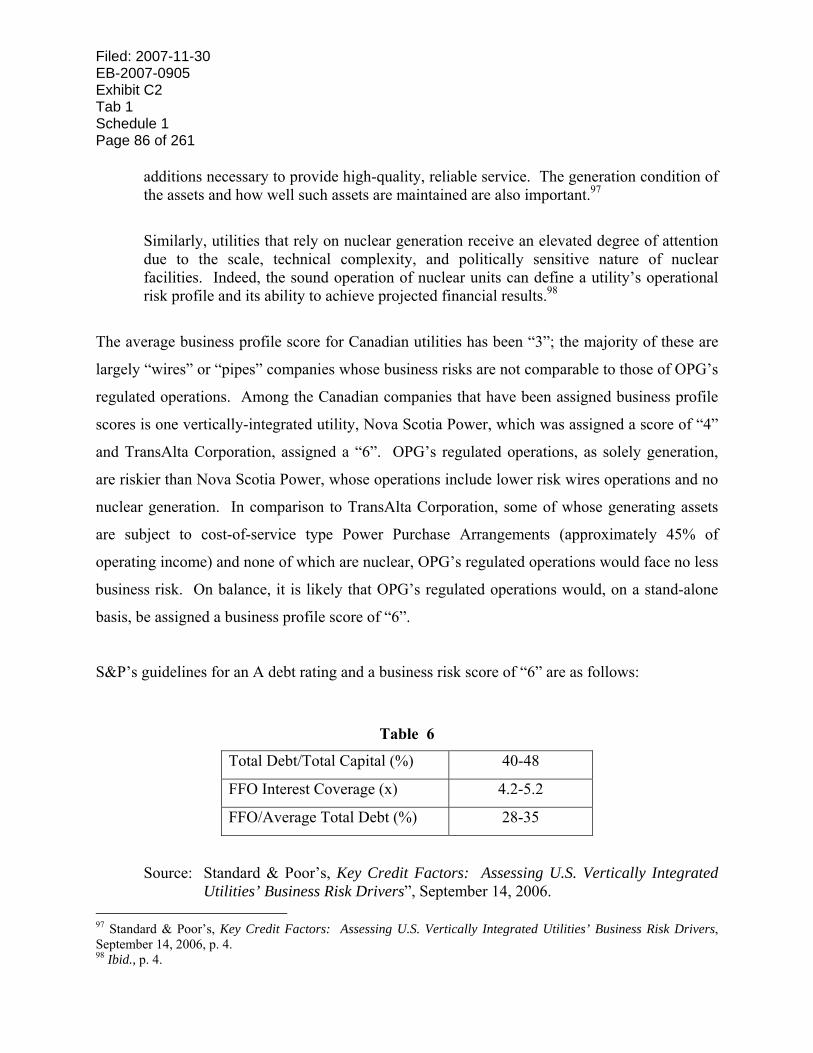
Filed: 2007-11-30 EB-2007-0905 Exhibit C2 Tab 1 Schedule 1 Page 86 of 261
additions necessary to provide high-quality, reliable service. The generation condition of the assets and how well such assets are maintained are also important.97
Similarly, utilities that rely on nuclear generation receive an elevated degree of attention due to the scale, technical complexity, and politically sensitive nature of nuclear facilities. Indeed, the sound operation of nuclear units can define a utility’s operational risk profile and its ability to achieve projected financial results.98
The average business profile score for Canadian utilities has been “3”; the majority of these are
largely “wires” or “pipes” companies whose business risks are not comparable to those of OPG’s
regulated operations. Among the Canadian companies that have been assigned business profile
scores is one vertically-integrated utility, Nova Scotia Power, which was assigned a score of “4”
and TransAlta Corporation, assigned a “6”. OPG’s regulated operations, as solely generation,
are riskier than Nova Scotia Power, whose operations include lower risk wires operations and no
nuclear generation. In comparison to TransAlta Corporation, some of whose generating assets
are subject to cost-of-service type Power Purchase Arrangements (approximately 45% of
operating income) and none of which are nuclear, OPG’s regulated operations would face no less
business risk. On balance, it is likely that OPG’s regulated operations would, on a stand-alone
basis, be assigned a business profile score of “6”.
S&P’s guidelines for an A debt rating and a business risk score of “6” are as follows:
Table 6
Total Debt/Total Capital (%) 40-48
FFO Interest Coverage (x) 4.2-5.2
FFO/Average Total Debt (%) 28-35
Source: Standard & Poor’s, Key Credit Factors: Assessing U.S. Vertically Integrated Utilities’ Business Risk Drivers”, September 14, 2006.
97 Standard & Poor’s, Key Credit Factors: Assessing U.S. Vertically Integrated Utilities’ Business Risk Drivers, September 14, 2006, p. 4. 98 Ibid., p. 4.
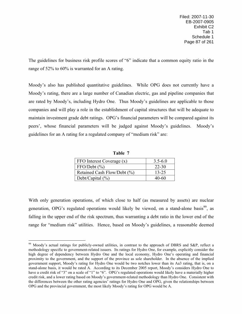
Filed: 2007-11-30 EB-2007-0905
Exhibit C2 Tab 1
Schedule 1 Page 87 of 261
The guidelines for business risk profile scores of “6” indicate that a common equity ratio in the
range of 52% to 60% is warranted for an A rating.
Moody’s also has published quantitative guidelines. While OPG does not currently have a
Moody’s rating, there are a large number of Canadian electric, gas and pipeline companies that
are rated by Moody’s, including Hydro One. Thus Moody’s guidelines are applicable to those
companies and will play a role in the establishment of capital structures that will be adequate to
maintain investment grade debt ratings. OPG’s financial parameters will be compared against its
peers’, whose financial parameters will be judged against Moody’s guidelines. Moody’s
guidelines for an A rating for a regulated company of “medium risk” are:
Table 7
FFO Interest Coverage (x) 3.5-6.0 FFO/Debt (%) 22-30 Retained Cash Flow/Debt (%) 13-25 Debt/Capital (%) 40-60
With only generation operations, of which close to half (as measured by assets) are nuclear
generation, OPG’s regulated operations would likely be viewed, on a stand-alone basis99, as
falling in the upper end of the risk spectrum, thus warranting a debt ratio in the lower end of the
range for “medium risk” utilities. Hence, based on Moody’s guidelines, a reasonable deemed
99 Moody’s actual ratings for publicly-owned utilities, in contrast to the approach of DBRS and S&P, reflect a methodology specific to government-related issuers. Its ratings for Hydro One, for example, explicitly consider the high degree of dependency between Hydro One and the local economy, Hydro One’s operating and financial proximity to the government, and the support of the province as sole shareholder. In the absence of the implied government support, Moody’s rating for Hydro One would be two notches lower than its Aa3 rating, that is, on a stand-alone basis, it would be rated A. According to its December 2005 report, Moody’s considers Hydro One to have a credit risk of “3” on a scale of “1” to “6”. OPG’s regulated operations would likely have a materially higher credit risk, and a lower rating based on Moody’s government-related methodology than Hydro One. Consistent with the differences between the other rating agencies’ ratings for Hydro One and OPG, given the relationships between OPG and the provincial government, the most likely Moody’s rating for OPG would be A.
Filed: 2007-11-30 EB-2007-0905 Exhibit C2 Tab 1 Schedule 1 Page 88 of 261 common equity ratio for OPG’s regulated operations compatible with a stand-alone A rating
would be in the range of 50-60%.
The common equity component alone does not determine the debt rating. Other financial
metrics, along with qualitative factors, are also taken into account by debt rating agencies. Thus,
for example, if a utility is able to achieve adequate ratios such as FFO Interest Coverage and
FFO/Debt ratios despite a debt ratio that is higher than indicated by guidelines (as a result of the
combination of ROE, cost of debt and cash flows from depreciation), it still may be able to
achieve an A rating. Consequently, S&P’s guideline range for the debt ratio is an important
indicator of an appropriate capital structure for OPG’s regulated operations, but other financial
metrics need to be taken into account. An analysis of stand-alone “notional”100 coverage ratios at
the benchmark return on equity of 10.5% and a common equity ratio of 57.5%, in the absence of
experiencing risks that cause the actual performance of the regulated operations to fall short of
expected levels, the principal cash flow metrics (FFO interest coverage and FFO to total debt) for
the regulated operations would be expected to be sufficient to achieve and maintain stand-alone
debt ratings in the A category.
F. CAPITAL STRUCTURES OF PEERS
The actual capital structures of OPG’s peers, which underpin those utilities’ debt ratings, may
also provide some insight into an appropriate stand-alone capital structure for an A rating. Since
there are no other regulated generation companies in North America, the closest peers for OPG’s
regulated operations would be, in Canada, TransAlta Utilities and TransAlta Corporation, and in
the U.S., electric utilities with S&P business profile scores of “6”.
100 The debt rating agencies do not calculate ratios for individual divisions of a company; they look at the ratios of the entity that raises capital. The notional ratios were estimated solely to test the impact of the combination of hypothetical capital structure and return on equity on the ability of the regulated operations to attract capital and maintain their creditworthiness on a stand-alone basis.
Filed: 2007-11-30 EB-2007-0905
Exhibit C2 Tab 1
Schedule 1 Page 89 of 261
TransAlta Corporation is rated BBB by both DBRS and S&P. TransAlta Utilities, the subsidiary
of TransAlta Corporation that holds the PPAs for the “heritage” Alberta generation, is rated
A(low) by DBRS and BBB+ by S&P. The debt ratio for TransAlta Corporation, as measured by
DBRS, has averaged 47.9% from 2003-2005; the corresponding debt ratio for TransAlta Utilities
has averaged 52.3%. The average ratios as measured by S&P for 2004-2006 were 53.2% for
TransAlta Corporation and 21.1% for TransAlta Utilities. The differences in the measurement of
the debt ratios for TransAlta Utilities by the two debt rating agencies relates primarily to the
treatment of preferred securities and preferred shares; DBRS treats TransAlta Utilities’ inter-
company preferred securities as 50% debt and the perpetual preferred shares as 30% debt, while
S&P treats both the preferred securities and shares as equity.101 The large proportion of
TransAlta Utilities’ capital structure that is made up of “hybrid” preferred securities makes it
difficult to draw definitive conclusions regarding a reasonable deemed debt/common equity
capital structure for OPG. Moreover, since the ratings of TransAlta Utilities are split (A(low) by
DBRS and BBB+ by S&P) and the ratings of TransAlta Corporation are both in the BBB
category, they provide some insight into what would be warranted for a BBB rating, but not for
an A rating. For a BBB rating, the TransAlta capital structures are indicative of a common
equity ratio (based solely on a debt/equity split) of approximately 50% for a generating
company.
With respect to U.S. companies, there are no A rated electric utilities with business profile scores
of “6”. The following table summarizes the debt ratios and other corresponding financial metrics
for the universe of electric utilities with rated debt.
101 Over 50% of TransAlta Utilities’ 2005 total capital, when defined as debt, preferred securities and common equity, was preferred securities.
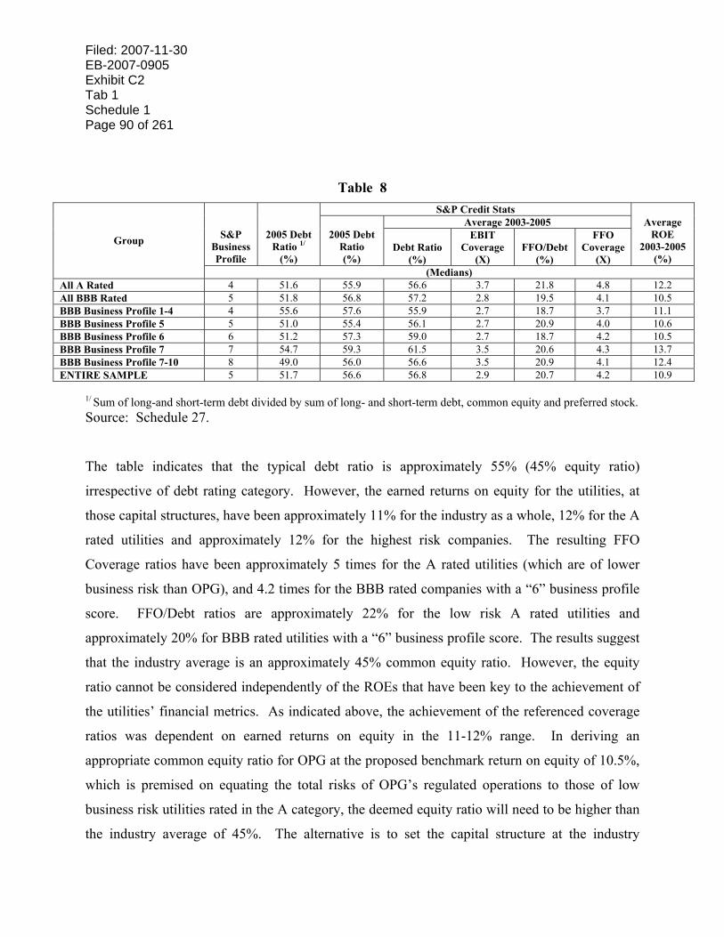
Filed: 2007-11-30 EB-2007-0905 Exhibit C2 Tab 1 Schedule 1 Page 90 of 261
Table 8 S&P Credit Stats
Average 2003-2005 S&P
Business Profile
2005 Debt Ratio 1/
(%)
2005 Debt Ratio (%)
Debt Ratio (%)
EBIT Coverage
(X) FFO/Debt
(%)
FFO Coverage
(X)
Average ROE
2003-2005 (%)
Group
(Medians) All A Rated 4 51.6 55.9 56.6 3.7 21.8 4.8 12.2 All BBB Rated 5 51.8 56.8 57.2 2.8 19.5 4.1 10.5 BBB Business Profile 1-4 4 55.6 57.6 55.9 2.7 18.7 3.7 11.1 BBB Business Profile 5 5 51.0 55.4 56.1 2.7 20.9 4.0 10.6 BBB Business Profile 6 6 51.2 57.3 59.0 2.7 18.7 4.2 10.5 BBB Business Profile 7 7 54.7 59.3 61.5 3.5 20.6 4.3 13.7 BBB Business Profile 7-10 8 49.0 56.0 56.6 3.5 20.9 4.1 12.4 ENTIRE SAMPLE 5 51.7 56.6 56.8 2.9 20.7 4.2 10.9
1/ Sum of long-and short-term debt divided by sum of long- and short-term debt, common equity and preferred stock. Source: Schedule 27.
The table indicates that the typical debt ratio is approximately 55% (45% equity ratio)
irrespective of debt rating category. However, the earned returns on equity for the utilities, at
those capital structures, have been approximately 11% for the industry as a whole, 12% for the A
rated utilities and approximately 12% for the highest risk companies. The resulting FFO
Coverage ratios have been approximately 5 times for the A rated utilities (which are of lower
business risk than OPG), and 4.2 times for the BBB rated companies with a “6” business profile
score. FFO/Debt ratios are approximately 22% for the low risk A rated utilities and
approximately 20% for BBB rated utilities with a “6” business profile score. The results suggest
that the industry average is an approximately 45% common equity ratio. However, the equity
ratio cannot be considered independently of the ROEs that have been key to the achievement of
the utilities’ financial metrics. As indicated above, the achievement of the referenced coverage
ratios was dependent on earned returns on equity in the 11-12% range. In deriving an
appropriate common equity ratio for OPG at the proposed benchmark return on equity of 10.5%,
which is premised on equating the total risks of OPG’s regulated operations to those of low
business risk utilities rated in the A category, the deemed equity ratio will need to be higher than
the industry average of 45%. The alternative is to set the capital structure at the industry

Filed: 2007-11-30 EB-2007-0905
Exhibit C2 Tab 1
Schedule 1 Page 91 of 261
standard, and to recognize OPG’s higher business risks relative to the benchmark in the common
equity return. Chapter IV.G following analyzes the trade-off between the equity ratio and the
return on equity.
G. CAPITAL STRUCTURE FOR OPG AT BENCHMARK RETURN102
In contrast to OPG’s regulated operations, which are 100% generation, the individual utilities
used to derive the benchmark return on equity are largely “wires” or “pipes” companies. Of the
seven individual Canadian utilities with publicly-traded stock103, and for which betas were
calculated, only three (Canadian Utilities, Emera and TransCanada) have any material generation
activities. Of these three, only one has any nuclear generation; TransCanada has a 47.9%
ownership stake in Bruce Power. The U.S. companies used to derive the benchmark return are
also largely low risk wires and pipes utilities. Of the 13 utilities in the benchmark U.S. utility
sample, only 5 are integrated electric utilities. The sample’s asset mix includes approximately
2.5% generation based on the median and 15.0% generation based on the average. The average
business profile score of the U.S. benchmark sample is “3”, compared to the typical generation
business profile score of “7” to “10”. The business profile scores that have been assigned to
Canadian utilities by S&P have averaged “3”; only two electricity firms, Emera/NSPI (“4”) and
TransAlta Corporation (“6”) have been assigned scores higher than “3”.
OPG’s regulated operations, 100% of which are generation, and approximately 45% of whose
regulated assets (65% of regulated generation capacity) are nuclear generation, are of
significantly higher risk than the utilities used to establish the benchmark return. As discussed in
Chapter III.A, the benchmark return is applicable to a typical, or average risk, Canadian utility.
For the benchmark return to be applicable to OPG’s regulated operations, the deemed capital
structure must be estimated that would equate OPG’s total (business plus financial) risks to those
102 A complete discussion of the methodology applied in this section is provided in Appendix I. 103 The seven utilities referenced are: Canadian Utilities, Emera, Enbridge, Fortis, Pacific Northern Gas, Terasen Inc. (stock has not been publicly-traded since its purchase by Kinder Morgan in November 2005), and TransCanada PipeLines.
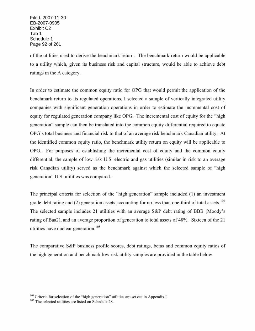
Filed: 2007-11-30 EB-2007-0905 Exhibit C2 Tab 1 Schedule 1 Page 92 of 261 of the utilities used to derive the benchmark return. The benchmark return would be applicable
to a utility which, given its business risk and capital structure, would be able to achieve debt
ratings in the A category.
In order to estimate the common equity ratio for OPG that would permit the application of the
benchmark return to its regulated operations, I selected a sample of vertically integrated utility
companies with significant generation operations in order to estimate the incremental cost of
equity for regulated generation company like OPG. The incremental cost of equity for the “high
generation” sample can then be translated into the common equity differential required to equate
OPG’s total business and financial risk to that of an average risk benchmark Canadian utility. At
the identified common equity ratio, the benchmark utility return on equity will be applicable to
OPG. For purposes of establishing the incremental cost of equity and the common equity
differential, the sample of low risk U.S. electric and gas utilities (similar in risk to an average
risk Canadian utility) served as the benchmark against which the selected sample of “high
generation” U.S. utilities was compared.
The principal criteria for selection of the “high generation” sample included (1) an investment
grade debt rating and (2) generation assets accounting for no less than one-third of total assets.104
The selected sample includes 21 utilities with an average S&P debt rating of BBB (Moody’s
rating of Baa2), and an average proportion of generation to total assets of 48%. Sixteen of the 21
utilities have nuclear generation.105
The comparative S&P business profile scores, debt ratings, betas and common equity ratios of
the high generation and benchmark low risk utility samples are provided in the table below.
104 Criteria for selection of the “high generation” utilities are set out in Appendix I. 105 The selected utilities are listed on Schedule 28.
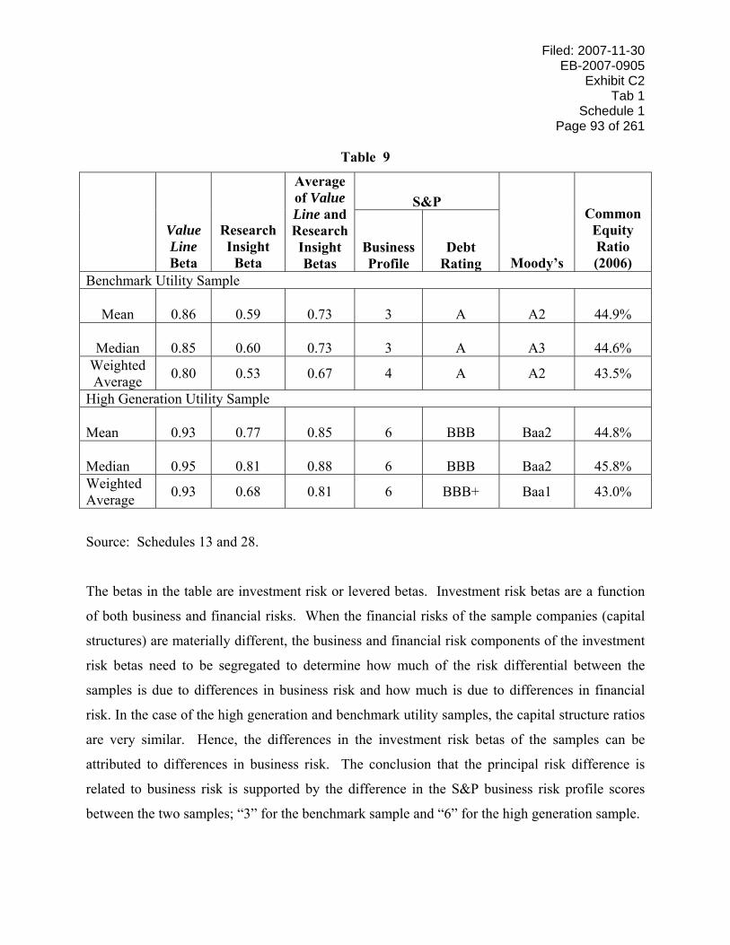
Filed: 2007-11-30 EB-2007-0905
Exhibit C2 Tab 1
Schedule 1 Page 93 of 261
Table 9
S&P
Value Line Beta
Research Insight
Beta
Average of Value Line and Research Insight Betas
Business Profile
Debt Rating Moody’s
Common Equity Ratio (2006)
Benchmark Utility Sample
Mean 0.86 0.59 0.73 3 A A2 44.9%
Median 0.85 0.60 0.73 3 A A3 44.6% Weighted Average 0.80 0.53 0.67 4 A A2 43.5%
High Generation Utility Sample
Mean 0.93 0.77 0.85 6 BBB Baa2 44.8%
Median 0.95 0.81 0.88 6 BBB Baa2 45.8% Weighted Average 0.93 0.68 0.81 6 BBB+ Baa1 43.0%
Source: Schedules 13 and 28.
The betas in the table are investment risk or levered betas. Investment risk betas are a function
of both business and financial risks. When the financial risks of the sample companies (capital
structures) are materially different, the business and financial risk components of the investment
risk betas need to be segregated to determine how much of the risk differential between the
samples is due to differences in business risk and how much is due to differences in financial
risk. In the case of the high generation and benchmark utility samples, the capital structure ratios
are very similar. Hence, the differences in the investment risk betas of the samples can be
attributed to differences in business risk. The conclusion that the principal risk difference is
related to business risk is supported by the difference in the S&P business risk profile scores
between the two samples; “3” for the benchmark sample and “6” for the high generation sample.
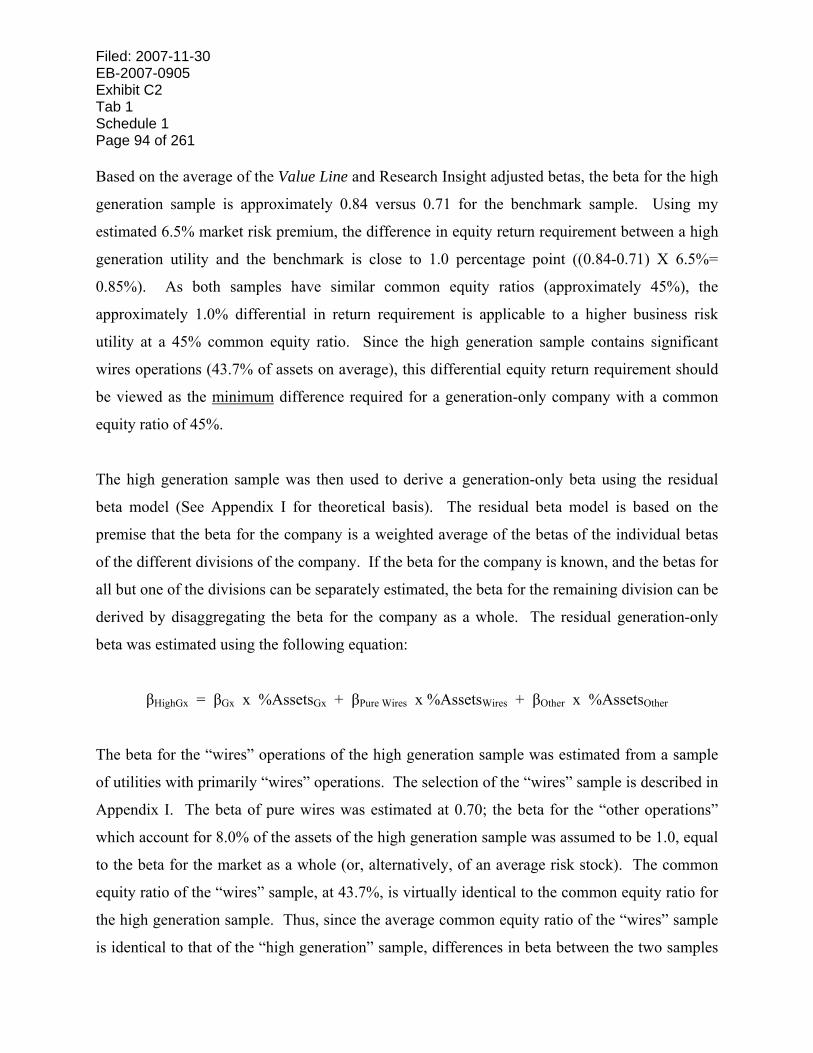
Filed: 2007-11-30 EB-2007-0905 Exhibit C2 Tab 1 Schedule 1 Page 94 of 261 Based on the average of the Value Line and Research Insight adjusted betas, the beta for the high
generation sample is approximately 0.84 versus 0.71 for the benchmark sample. Using my
estimated 6.5% market risk premium, the difference in equity return requirement between a high
generation utility and the benchmark is close to 1.0 percentage point ((0.84-0.71) X 6.5%=
0.85%). As both samples have similar common equity ratios (approximately 45%), the
approximately 1.0% differential in return requirement is applicable to a higher business risk
utility at a 45% common equity ratio. Since the high generation sample contains significant
wires operations (43.7% of assets on average), this differential equity return requirement should
be viewed as the minimum difference required for a generation-only company with a common
equity ratio of 45%.
The high generation sample was then used to derive a generation-only beta using the residual
beta model (See Appendix I for theoretical basis). The residual beta model is based on the
premise that the beta for the company is a weighted average of the betas of the individual betas
of the different divisions of the company. If the beta for the company is known, and the betas for
all but one of the divisions can be separately estimated, the beta for the remaining division can be
derived by disaggregating the beta for the company as a whole. The residual generation-only
beta was estimated using the following equation:
βHighGx = βGx x %AssetsGx + βPure Wires x %AssetsWires + βOther x %AssetsOther
The beta for the “wires” operations of the high generation sample was estimated from a sample
of utilities with primarily “wires” operations. The selection of the “wires” sample is described in
Appendix I. The beta of pure wires was estimated at 0.70; the beta for the “other operations”
which account for 8.0% of the assets of the high generation sample was assumed to be 1.0, equal
to the beta for the market as a whole (or, alternatively, of an average risk stock). The common
equity ratio of the “wires” sample, at 43.7%, is virtually identical to the common equity ratio for
the high generation sample. Thus, since the average common equity ratio of the “wires” sample
is identical to that of the “high generation” sample, differences in beta between the two samples
Filed: 2007-11-30 EB-2007-0905
Exhibit C2 Tab 1
Schedule 1 Page 95 of 261
can be attributed to differences in business risk (i.e., there is no need to segregate the investment
risk betas of the “wires” sample into business and financial risks components). Using the
formula and betas above, the derived beta for generation-only was estimated at 0.94. The
difference in the equity return requirement between generation and a benchmark utility can then
be estimated as approximately 1.5%, calculated as the difference in betas multiplied times the
market risk premium ((0.94-0.71) X 6.5% = 1.5%). As with the estimation of the return
requirement differential based on the high generation sample compared to the benchmark
sample, the 1.5% applies to a generation-only company with a similar common equity ratio, that
is, 45%.
Because OPG’s regulated operations are 100% generation, the incremental equity returns at a
45% equity ratio are at the upper end of the range, i.e. in the range of approximately 1.25% to
1.50%. This incremental equity return was then used to develop the range of equity ratios for
OPG’s regulated operations that would be required to equate the fair return for OPG’s regulated
operations to the benchmark return of 10.5%. The quantification of the common equity ratio
range was based on the application of two capital structure theories.
Theory 1 posits that income taxes and the deductibility of interest for corporate income tax
purposes have no impact on the cost of capital. Under this theory, the overall cost of capital
stays constant when the capital structure changes, although the costs of the debt and equity
components change (i.e., the cost of equity rises when the equity ratio declines). Theory 2 posits
that income taxes and the corporate deductibility of interest expense cause the overall cost of
capital to continually decline as the equity ratio declines and the debt ratio increases. The actual
impact on the cost of capital most likely lies in between the results of the two theories; income
taxes and the deductibility of interest do tend to decrease the cost of capital (as the income trust
market has demonstrated), but as the debt ratio rises, there are increasing costs in terms of loss of
financing flexibility and potential bankruptcy. Moreover, in the case of regulated companies, the
benefit of the tax deductibility of interest is to the benefit of ratepayers, while in the unregulated
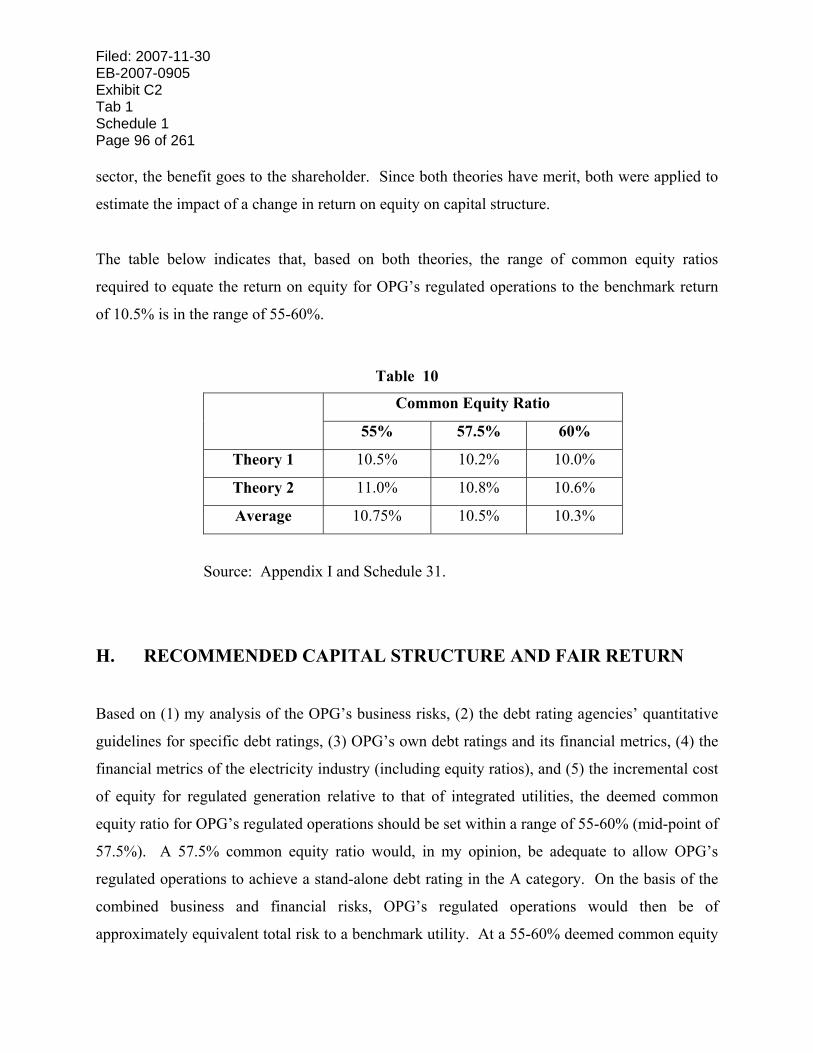
Filed: 2007-11-30 EB-2007-0905 Exhibit C2 Tab 1 Schedule 1 Page 96 of 261 sector, the benefit goes to the shareholder. Since both theories have merit, both were applied to
estimate the impact of a change in return on equity on capital structure.
The table below indicates that, based on both theories, the range of common equity ratios
required to equate the return on equity for OPG’s regulated operations to the benchmark return
of 10.5% is in the range of 55-60%.
Table 10
Common Equity Ratio
55% 57.5% 60%
Theory 1 10.5% 10.2% 10.0%
Theory 2 11.0% 10.8% 10.6%
Average 10.75% 10.5% 10.3%
Source: Appendix I and Schedule 31.
H. RECOMMENDED CAPITAL STRUCTURE AND FAIR RETURN
Based on (1) my analysis of the OPG’s business risks, (2) the debt rating agencies’ quantitative
guidelines for specific debt ratings, (3) OPG’s own debt ratings and its financial metrics, (4) the
financial metrics of the electricity industry (including equity ratios), and (5) the incremental cost
of equity for regulated generation relative to that of integrated utilities, the deemed common
equity ratio for OPG’s regulated operations should be set within a range of 55-60% (mid-point of
57.5%). A 57.5% common equity ratio would, in my opinion, be adequate to allow OPG’s
regulated operations to achieve a stand-alone debt rating in the A category. On the basis of the
combined business and financial risks, OPG’s regulated operations would then be of
approximately equivalent total risk to a benchmark utility. At a 55-60% deemed common equity
Filed: 2007-11-30 EB-2007-0905
Exhibit C2 Tab 1
Schedule 1 Page 97 of 261
ratio, the fair return for OPG’s regulated operations is equal to the benchmark return on equity of
10.5%.
I. IMPLIED CAPITAL STRUCTURE OF OPG’S UNREGULATED OPERATIONS
The objective of adherence to the stand-alone principle for purposes of determining the deemed
capital structure and return on equity is to ensure that ratepayers are bearing a cost of capital that
represents the risks of the regulated activities of the firm, not the risks of the consolidated
operations. An element of the application of the stand-alone principle is ensuring that the
regulated operations are not subsidizing unregulated operations. A cross-subsidy can be said to
exist if the regulated operations are bearing costs that are the responsibility of the unregulated
operations.
Since the proposed deemed common equity ratio for the regulated operations of 57.5% is lower
than OPG’s 2006 consolidated equity ratio as reflected in OPG’s audited financial statements,
assuming the consolidated equity ratios were maintained, the implied unregulated operations’
common equity ratio is higher than the proposed deemed ratio for regulated operations. Further,
the profitability of the consolidated operations and the individual business segments since the
implementation of the Electric Restructuring Act 2004 indicate that the unregulated segment has
been largely responsible for the improved financial position of OPG. As reported by DBRS, the
return on equity for the consolidated operations was 11.7% in 2005 compared to the ROE of
5.0% on the prescribed assets. The unregulated operations, which account for approximately
one-third of the assets, contributed over 50% of the operating income in both 2005 and 2006 as
per OPG’s audited financial statements.

Filed: 2007-11-30 EB-2007-0905 Exhibit C2 Tab 1 Schedule 1 Page 98 of 261
Given that the unregulated operations – which are comprised largely of coal, oil/gas, hydro and
wind generation – add to the diversification of OPG’s overall portfolio of generation, contribute
more than 50% of the operating income of the operations (even with a revenue cap in place), and
have an implied common equity ratio slightly higher than that proposed for the regulated
operations, there is no basis for any concern that, with a deemed common equity ratio of 57.5%,
the regulated operations would be subsidizing the unregulated operations.
Filed: 2007-11-30 EB-2007-0905
Exhibit C2 Tab 1
Schedule 1 Page 99 of 261
V. CAPITAL MARKET VIEWS ON FAIR RETURN/CAPITAL
STRUCTURE
A. IMPLICATIONS OF GLOBALIZATION OF CAPITAL MARKETS
With the potential for refurbishment of existing nuclear units and construction of new nuclear
units, OPG could be facing unprecedented capital expenditures for regulated generation over the
next 20 years. As noted earlier, OPA has estimated that the plan to ensure the reliability of the
Ontario’s electricity supply could cost approximately $60 billion, of which approximately $26
billion could be for refurbishment of existing nuclear units and construction of new units.106
OPG would not be alone in facing large capital expenditures. In its 2003 World Energy
Investment Outlook, the International Energy Agency estimated that over $1.5 trillion in
investment would be required by the electricity industry in North America. OPG will thus be
competing for capital in a market that may be characterized by an unprecedented requirement for
debt capital by a single industry. To compete successfully in the public debt markets, that is, to
be able to attract capital on flexible terms and conditions, OPG will require financial metrics that
are compatible with its peers on a risk-adjusted basis. Its peers are increasingly global, not solely
Canadian.
Globalization of the capital markets has been a gradual phenomenon, as information barriers and
transactions costs have declined, and financial reporting has become more standardized. The
repeal of the Foreign Property Rule (FPR) in Canada in August 2005 has eliminated a further
barrier, effectively releasing investment that was previously captive. Comparisons among
companies across boundaries have become increasingly common. For example, S&P’s peer
106 The forecast costs for nuclear refurbishment and new build are not specific to OPG.
Filed: 2007-11-30 EB-2007-0905 Exhibit C2 Tab 1 Schedule 1 Page 100 of 261 comparison for OPG includes two Canadian companies (TransAlta and Emera) and a U.S.
company, Exelon.107 With investors more willing to invest capital across international
boundaries, a regulated company’s ability to offer a return that is compensatory with its risk and
comparable to its peers’ becomes an increasingly imperative objective.
In the U.S., the average return on equity allowed for electric utilities by state regulators from the
beginning of 2003 to the end of the second quarter of 2007, during which the long-term U.S.
Treasury bond yield averaged 4.9% – virtually identical to the forecast 2008 5.0% long Canada
yield – was 10.6% on a common equity ratio of 47.7%. The approved returns and capital
structures are for both “wires” only (transmission/distribution companies) and vertically
integrated companies, both of which would be less risky than OPG, whose regulated operations
are generation-only. At the U.S. federal level, the Federal Energy Regulatory Commission
(FERC) sets returns and capital structures for electricity transmission, for which the recent
allowed “baseline” returns on equity have been in the range of 10.8%-12.4% on equity ratios in
the 50-60% range. Baseline returns are exclusive of incentives. Since generation is riskier than
transmission, the FERC returns would be supportive of returns in excess of 11-12%.108
107 TransAlta’s peers are PPL Corp and Constellation Energy, both U.S. companies. 108 The Conference Board of Canada has pointed out the importance of competitive returns for transmission in Canada. In its May 2004 Briefing entitled, “Electricity Restructuring: Opening Power Markets”, the Conference Board stated,
Investors are discouraged by limitations on the regulated cost recovery for transmission upgrading. Transmission companies are simply not seeing favourable risk/return ratios on their investments, and know that they can realize better returns in the United States, where regulated rates of return are much higher. Rates of return to Canadian firms for transmission projects are around 9 to 10 per cent, well below the 13 to 14 per cent available to U.S. companies. These lower rates discourage investment in Canadian utilities. Moreover, investors are additionally deterred by the fact that existing cost-of-service rates do not reflect the economic value of the transmission grid.
That conclusion would be no less true for regulated generation.
Filed: 2007-11-30 EB-2007-0905
Exhibit C2 Tab 1
Schedule 1 Page 101 of 261
B. VIEWS OF CANADIAN DEBT RATING AGENCIES
As indicated in Chapter III.D, debt rating agencies and debt investors look at a variety of
quantitative financial measures in assessing the financial strength of a regulated company. For a
regulated utility, the ability to achieve strong financial metrics arises not only from the equity
component, but also the return allowed on that equity component and the rate of depreciation.
Both DBRS and S&P have consistently commented on the highly levered nature of Canadian
utilities and the low allowed common equity returns relative to their global peers, particularly
those in the U.S.
DBRS has noted that it would like to see both the deemed common equity ratios and allowed
returns increased to levels more consistent with U.S. returns. 109
In December 2004, subsequent to the AEUB’s Generic Cost of Capital Decision (2004-052,
dated July 2004), DBRS referred to the low deemed equity and returns as a “challenge” for the
ATCO Utilities. The DBRS report for ATCO Ltd. stated,
While ATCO’s diversified operations, coupled with the Company’s prudent management approach, provide a level of earnings stability, additional challenges over the medium term include the relatively low approved returns on equity (ROE) and deemed equity for the regulated businesses, continuing regulatory risk and lag and ATCO’s merchant power exposure in Alberta.
Additional recent DBRS reports citing the challenge of low approved returns on equity have
been published for other Alberta utilities, i.e., AltaLink (November 2004), and FortisAlberta
(September 2004).
As previously noted, IV.D.1, DBRS has commented with specific reference to OPG, that
regulated vertically integrated utilities in the U.S. have deemed capital structures ranging from 109 DBRS, The Rating Process and the Cost of Capital for Utilities: Five Reasons Why Canadian Utilities have Lower Ratios and Five Changes to Regulation Which Should be Introduced in Canada, May 2003.
Filed: 2007-11-30 EB-2007-0905 Exhibit C2 Tab 1 Schedule 1 Page 102 of 261 35% common equity to 55% common equity and have an approved ROE ranging from 9.75% to
13.5%. A comparable entity to OPG (that is, one without stable transmission and distribution
operations), according to DBRS, would be near the top of both ranges.
With respect to Standard & Poor’s, in early March 2003, the debt rating agency announced that it
was re-evaluating its prior justification of the strong investment grade ratings of Canadian
utilities (i.e., the nature of Canadian regulation).
S&P noted that Canadian utilities are among the most highly levered utilities in their global
ratings universe, and that the highly leveraged financial profiles generally stem from regulatory
directives. Subsequent to that announcement, S&P has commented on the low equity ratios and
allowed returns of specific Canadian utilities.
For example, like DBRS, S&P has made references to the low level of equity ratios allowed in
the EUB’s Generic Cost of Capital decision for other Alberta utilities. Subsequent to the EUB
decision, S&P commented on the thin equity layers allowed the ATCO group of utilities, stating,
The regulatory regime, although comparable with other provinces in Canada, typically approves less generous returns on thinner equity layers than those approved for ATCO’s global peers. Approved returns for ATCO’s regulated businesses are 9.6% on equity layers varying from 33%-43% of total capital. (S&P, Research Update: ATCO Group of Companies ‘A’ Ratings Affirmed; Outlook Stable, November 9, 2004.)
In a relatively recent report for AltaLink (rated A-), S&P stated,
Like many regulated utilities in Canada, AltaLink's average financial profile is constrained by a comparatively low approved ROE (8.93% in 2006) on a thin deemed equity base of 35%. (S&P, Research Summary: AltaLink, June 5, 2006)
Filed: 2007-11-30 EB-2007-0905
Exhibit C2 Tab 1
Schedule 1 Page 103 of 261
In its report for Union Gas issued subsequent to the utility’s 2006 settlement in which the
allowed common equity ratio was raised to 36%, the two weaknesses referred to by S&P were
the high leverage associated with company's regulated capital structure and the relatively low
allowed ROE compared with global peers (S&P, Research: Union Gas, August 24, 2006).
In general, S&P considers that Canadian utility financial polices tend to be aggressive with
leverage, and regulators parsimonious with returns.110 As noted above, the “aggressive leverage”
is largely a result of regulatory directives.
C. VIEWS OF EQUITY ANALYSTS
Canadian equity analysts rarely comment on the level of allowed returns and capital structures of
regulated companies. However, there have been some notable exceptions. As long ago as
December 2001, CIBC World Markets Report entitled “Pipelines and Utilities: Time to Lighten
Up”, stated, in reference to the then recent formulaic reduction in Newfoundland Power’s
allowed return (from 9.59% to 9.05% year over year):
The magnitude of the reduction in the case of Newfoundland Power illustrates the flaw in using a brief snapshot of existing rates rather than a forecast of rates that are expected to persist during the upcoming year. More importantly, however, it shows the shortcoming of the formula approach itself. Mechanically tying allowed returns on equity to long bond yields is an approach that is simple for regulators to apply; however, in recent years, with a steady decline in bond yields, it has produced-allowed returns that are out of sync with the cost of capital, and returns that are being achieved with comparable nonregulated companies or regulated returns that are achievable in the U.S.
At the time of the report, the allowed returns for Canadian utilities were approximately 9.6%,
compared to just over 11% for U.S. utilities.
110 Standard & Poor’s, Industry Report Card: Regulatory Rulings, M&A, and Fuel Cost Recovery Dominate Global Utilities Credit Environment, November 21, 2006.

Filed: 2007-11-30 EB-2007-0905 Exhibit C2 Tab 1 Schedule 1 Page 104 of 261 In the NEB’s August 2005 Canadian Hydrocarbon Transportation System report, as noted
above, pension funds had indicated to the Board that the basic financial parameters (allowed
return on equity and deemed capital structure) in its regulatory scheme should be improved. In
its 2006 report of the same name, the NEB reported that a number of analysts felt that the ROE
generated by the NEB formula and by other Canadian regulators’ formulas “were a little too
low” and not supportive of dividend growth or credit metrics. A number of analysts commented
that where they have “Buy” recommendations on utility stocks, the recommendations tend to
reflect the prospects of the unregulated operations.111 Analysts also commented that companies
have reduced costs and taken other steps to improve profitability and dividend growth for several
years, and wondered how long that could continue. The 2007 Report expressed similar views.
Some parties expressed concern that the stand-alone pipelines might have difficulty attracting
capital given low ROEs. Others felt the regulated entities would be able to attract capital, but
that the terms under which they did so would be more costly than for the consolidated entity. In
addition, the report stated that,
Many analysts expressed support for a formulaic approach to determining ROEs because of the transparency, stability and predictability that this method provides. However, a number expressed the view that the ROE resulting from the formula was too low, and contend that they are much lower than regulated ROEs in the U.S. and U.K. While views ranged widely on this issue, some felt that the typically lower ROEs in Canada were not justified by the differences in risk for Canadian companies compared to FERC-regulated pipelines. Some parties suggested it was time for the Board to revisit the ROE Formula.
The most recent analyst commentary on the level of allowed ROEs in Canada expresses the view
that the current level of allowed ROEs, expected to be approximately 8.6% in 2007, is now
confiscatory. Specifically, in Pipelines/Gas & Electric Utilities, dated December 7, 2006, Karen
Taylor, equity analyst for BMO Capital Markets, concluded:
111 In many cases, the ROEs achieved by the entity whose shares are traded have been materially higher than the ROEs allowed under the formulas. The allowed ROE generated by the NEB formula averaged 9.6% over the period 2002 to 2005; the ROE reported for TransCanada Pipelines Ltd by DBRS over that same period was 12.7%. For Terasen Gas, its allowed ROE averaged 9.2%; Terasen Inc.’s ROE (as reported by DBRS) averaged 11.1%. DBRS reported an average ROE of 13.0% for Canadian Utilities Ltd., compared to its regulated subsidiaries’ allowed ROEs of approximately 9.6%.
Filed: 2007-11-30 EB-2007-0905
Exhibit C2 Tab 1
Schedule 1 Page 105 of 261
We believe that regulators have consistently refused to give weight to a number of arguments that would result in higher allowed returns, solely on the basis that to do so would result in higher customer rates.
● The North American capital markets are increasingly integrated and investors have the ability to invest in utility assets north and south of the border.
● There is merit incorporating U.S. market metrics into the analysis and that the Canadian benchmark equity portfolio (the S&P/TSX) may not meet the theoretical requirement for a diversified market portfolio.
● The returns on comparable investments with similar risk, whether they be Canadian or U.S. examples, should be considered.
● The allowed return on equity and deemed equity must satisfy all aspects of the Fair Return Standard and that no part of the Standard has priority. ….
● No pipeline or energy utility in our regulated coverage universe has issued equity in the last five years to fund, on an unlevered basis, a dollar-for-dollar equity investment in utility rate base. Continued assertions by regulators that utilities have adequate access to capital are not credible with respect to the equity component, as access to equity has not been tested over the ensuing period. ….
● Continued investment in utility rate base by the owners of utilities is not an acquiescence that the allowed return on equity is appropriate and that investment may relate to other obligations including the utility’s obligation to be the supplier or supply of last resort and fulfill the obligation to serve, maintain the safe and reliable operation of the utility, and may be fulfilling specific conditions of its operating licence. ….
● A failure by utility companies to annually litigate the allowed return on equity “formula” does not constitute acceptance of the adequacy of the allowed return. Rather, we believe that the lack of annual litigation reflects the cost of the process, the time required to pursue litigation that detracts from management’s ability to focus on the efficient operation of the business and the potential damage to important utility regulatory and customer relationships. ….
● The evidenciary standard is too high and almost impossible to meet. Moreover, we believe that notwithstanding decisions from the Supreme Court that stipulate otherwise, utility regulators continue to rely heavily on their quasi-judicial and expert status to impose a bare-bones return on equity and drive down the deemed capital structure of the utility in order to protect customers from prices, without the fear of reconsideration upon appeal. Regulators must establish the cost of equity and deemed equity not because they are experts in this regard, but in order to establish just and reasonable rates. The regulator is not permitted to consider the effects
Filed: 2007-11-30 EB-2007-0905 Exhibit C2 Tab 1 Schedule 1 Page 106 of 261
on customers in the determination of the allowed ROE and capital structure, and we do not believe that the regulator is permitted to factor in other policy objectives into its determination of the allowed return on equity; i.e., we do not believe that the regulator is permitted to reduce the allowed return on equity and/or deemed equity for small utility companies in other to encourage consolidation or any other specific policy objective. We believe in these situations, that the inclusion of these other factors in the assessment of cost of equity and designation of deemed equity, unlawfully transfers value to utility ratepayers from its legitimate owner, the utility shareholders.
In sum, the returns available to comparable U.S. utilities are materially higher than the returns
that are allowed to Canadian utilities, the returns allowed for Canadian utilities are generally
regarded as too low, and the returns that investors expect and are achieving from the traded
entities in Canada are considerably higher than the returns that have been allowed by regulators.
These factors are legitimate considerations to be taken into account in setting a fair and
reasonable return for OPG’s regulated operations.
Filed: 2007-11-30 EB-2007-0905
Exhibit C2 Tab 1
Schedule 1 Page 107 of 261
VI. AUTOMATIC ADJUSTMENT MECHANISM
The key purpose of automatic adjustment mechanisms for return on equity (ROE) is to avoid
annual reviews of the allowed return on equity. The appropriate return on equity is unobservable
(in contrast to the cost of debt) and is subject to a wide difference of opinion. Testimony on the
fair return is typically technical and lengthy, and often quite similar from year to year.
Considerable time, effort and money are spent on testimony preparation, information requests,
and cross-examination. An automatic adjustment mechanism is a means of avoiding annual
ROE reviews, while providing timely changes in the allowed return on equity. Since OPG is
likely to face a number of limited issue hearings over the next several years, with ROE assigned
to the first, the consideration of an automatic adjustment mechanism is particularly germane.
The ROE can be set in the first proceeding, with no further need to address the issue throughout
the remaining limited issues proceeding.
An automatic adjustment mechanism for ROE is relied upon in six different regulatory
jurisdictions in Canada. The OEB first introduced an automatic adjustment mechanism in 1997
for the natural gas utilities; it approved automatic adjustment mechanisms for Hydro One and the
electricity distributors in 1998 and 1999 respectively. The Board’s automatic adjustment
mechanism for the gas distributors was reviewed in detail in 2003 and reconfirmed in early 2004.
In its Report to the Board on Cost of Capital and 2nd Generation Incentive Regulation for
Ontario’s Electricity Distributors, issued December 20, 2006, the Board has retained the existing
automatic adjustment mechanism for the electricity distributors as part of its guidelines for
setting rates for 2007-2009.
The automatic adjustment mechanisms currently operating in Canada are all quite similar. The
point of departure for the implementation of each of the automatic adjustment mechanisms was

Filed: 2007-11-30 EB-2007-0905 Exhibit C2 Tab 1 Schedule 1 Page 108 of 261 the determination of a “base” or initial ROE and its two component parts, the risk-free rate and
the equity risk premium. The adjustment mechanism itself specifies how changes from the base
ROE are to be calculated for subsequent years. The two major components of the adjustment
mechanism are the measurement of the risk-free rate and the formula to be used to adjust the
ROE from one year to the next. The yield on the benchmark long-term (30-year) Government of
Canada bond is used as the proxy for the risk-free rate.
The methodology used by the OEB has two components, the “initial setup” and the “adjustment
mechanism”. The “initial setup” has two steps: (1) establish the forecast of the long-term
Canada yield for the test year and (2) establish the implied risk premium. The “adjustment
mechanism” also has two steps: (1) establish the forecast long Canada rate and (2) apply the
adjustment factor. The adjustment factor was specified in the Guidelines at 0.75. The
adjustment factor of 0.75 means that the allowed ROE changes by 75% of the change in the
forecast long-term Government of Canada bond yield. The same 75% adjustment mechanism is
used by four of the other five regulators that rely on automatic adjustment mechanisms.
The key advantages of an automatic adjustment mechanism are as follows:
1. It reduces the regulatory burden imposed by the annual determination of ROEs.
2. It results in increased predictability of the allowed returns;
3. It avoids any potential arbitrariness of the outcome.
The principal disadvantages include:
1. There are constraints placed on the regulator’s flexibility in setting the allowed return to
address issues such as financing flexibility requirements;
Filed: 2007-11-30 EB-2007-0905
Exhibit C2 Tab 1
Schedule 1 Page 109 of 261
2. If the base return is inadequate or excessive, the operation of the formula could
potentially compound problems with the initial ROE;
3. If the formula adopted does not appropriately track changes in the cost of equity,
subsequent allowed ROEs may not be representative of a fair return, and potentially, an
impairment of financing flexibility.
4. There is a potential for more volatility in the regulated payments if the ROE changes
materially from year-to-year than if the ROE remains unchanged for an extended period.
5. Some parties believe that the use of an automatic adjustment formula based on changes in
the risk-free rate requires that the base ROE be determined solely on the basis of the
equity risk premium test.
If there are sufficient safeguards in place that permit the formula to be revisited or that permit the
utility to seek relief in circumstances of financial distress, the principal disadvantages of an
automatic adjustment formula can be overcome. Moreover, financial flexibility concerns can be
addressed through a change in the deemed capital structure. While DBRS has called the
sensitivity of Canadian utilities’ earnings to interest rates a “Challenge”, the experienced year-to-
year changes in formula-driven ROEs do not individually have a major negative impact on
interest coverage. However, a steady decline in ROEs over a number of years will have (and has
had) a cumulative impact, largely because the embedded cost of debt declines more slowly than
allowed ROEs.
With respect to any concerns that the automatic adjustment mechanism sacrifices the
contribution of tests other than the equity risk premium test, that concern is misplaced. The
reliance on an interest rate to adjust the ROE from year to year, does not exclude, for purposes of
setting the initial return, reliance on tests whose formulation does not include an interest rate. In
this regard, I note that the BCUC and the AEUB, when setting the base return in their recent
Filed: 2007-11-30 EB-2007-0905 Exhibit C2 Tab 1 Schedule 1 Page 110 of 261 “generic” cost of capital decisions (2006 and 2004 respectively), looked at all of the tests and
market information on their own merits, not whether they were based on the same parameters as
the proposed automatic adjustment formula.
I recommend the adoption of an automatic adjustment formula for OPG, recognizing that a key
to its success is the Board’s adoption of a reasonable initial return.112 With respect to the
specifics of the adjustment mechanism, the Board’s existing formula for subsequent changes in
ROE, that is, a 75 basis point change in ROE for every one percentage point change in the
forecast 30-year Canada bond yields, remains a reasonable approximation of the relationship
between cost of equity and interest rates. However, OPG should retain the right to seek a review
of the formula if there is evidence that the formula itself is not producing returns that will allow
OPG to attract capital on reasonable terms (e.g., a threat of a downgrade to non-investment
grade, assuming that threat can be tied, at least in part, to regulated operations).
As a further protection, I recommend that the formula should be reviewed if forecast long
Canada bond yields fall below 3.0% or exceed 8.0%. Long Canada yields outside of the range of
3.0%-8.0% may indicate a materially altered relationship between long Canada bond yields and
the utility cost of equity. The specification of 3.0% as the bottom end of the range recognizes
there has been no experience with long-term Canada yields near this level since the early 1950s.
With respect to the upper end of the range, if long Canada bond yields were to reach 8.0%, the
real cost of capital or inflation would be materially higher than that which is currently
anticipated. Both circumstances would warrant a review of the validity of the formula.
112 The importance of the internal consistency between the initial return and the automatic adjustment formula must be underscored. It would be unreasonable for the Board to allow a return on equity that implicitly assumes that the cost of equity has declined by 100% of the decline in interest rates since the persistent downward trend began in 1995, but then impose a formula that only increases the allowed return by 75% of future increases in interest rates.
Filed: 2007-11-30 EB-2007-0905
Exhibit C2 Tab 1
Schedule 1 Page 111 of 261
APPENDICES TO
Capital Structure and Fair Return on Equity
Prepared for
ONTARIO POWER GENERATION
Prepared by
KATHLEEN C. McSHANE
FOSTER ASSOCIATES, INC.
November 2007
Filed: 2007-11-30 EB-2007-0905 Exhibit C2 Tab 1 Schedule 1 Page 112 of 261
APPENDICES
Page A. DEEMED VERSUS ACTUAL CAPITAL STRUCTURE 113 B. THE CAPITAL ATTRACTION AND COMPARABLE EARNINGS
STANDARDS 124 C. RISK-ADJUSTED EQUITY MARKET RISK PREMIUM TEST 129 D. DCF-BASED RISK PREMIUM TEST 159 E. DISCOUNTED CASH FLOW TEST 161 F. COMPARABLE EARNINGS TEST 168 G. FINANCING FLEXIBILITY ADJUSTMENT 181 H. DEBT RATING AGENCY FINANCIAL METRIC GUIDELINES 187 I. TRANSLATION OF RETURN REQUIREMENT TO COMMON
EQUITY RATIO 189 J. QUALIFICATIONS OF KATHLEEN C. McSHANE 202
Filed: 2007-11-30 EB-2007-0905
Exhibit C2 Tab 1
Schedule 1 Page 113 of 261
______________________________________________________________________________ Appendix A
APPENDIX A
DEEMED VERSUS ACTUAL CAPITAL STRUCTURE
DEFINITION OF DEEMED CAPITAL STRUCTURE
The term deemed, or hypothetical, capital structure, simply refers to imputing, for ratemaking
purposes, a capital structure that is different from the capital structure that is reported on the
utility’s financial statements or forecast to be reported on the financial statements during the test
period. The most common method of applying the deemed capital structure construct is to:
1. estimate the rate base;
2. apply to the rate base a pre-determined percentage of common equity;
3. attribute to the regulated operations actual outstanding and forecast issues of long-term
debt and preferred shares; and
4. to the extent that the rate base and the sum of the deemed common equity and the
available actual long-term debt and equity do not match, balance the rate base and capital
structure with a “plug”, either debt (if rate base is greater than capitalization) or notional
investments (if capitalization is greater than rate base).

Filed: 2007-11-30 EB-2007-0905 Exhibit C2 Tab 1 Schedule 1 Page 114 of 261
______________________________________________________________________________ Appendix A
HISTORY OF DEEMED CAPITAL STRUCTURE IN CANADA
Deemed capital structures have been used in Canada since at least 1978. The Ontario Energy
Board has relied on deemed capital structures for the local gas distribution utilities it regulates
since at least 1981.113 The use of deemed capital structures arose in the context of applying what
has been referred to as the stand-alone principle. Adherence to the stand-alone principle requires
setting a capital structure and cost of capital that reflect the risks of the regulated utility as a
stand-alone entity, not those of the legal entity within which the regulated utility resides.114 The
perceived need for reliance on deemed capital structures was primarily the result of the extent to
which regulated companies were diversified into operations whose risks were significantly
different from those of their regulated operations. The consolidated capital structure and cost of
capital were thus viewed as not representative of the capital structures the regulated entity would
maintain on a stand-alone basis or of the cost of capital the regulated entity would face on a
stand-alone basis. The stand-alone capital structure and return on rate base were intended to
113 In EBRO 376-I & II (January 30, 1981), the OEB approved a stand-alone capital structure for Consumers Gas (now Enbridge Gas Distribution). 114 The Alberta Energy and Utilities Board (EUB) described the stand-alone principle as follows:
This first application of the stand-alone principle is designed to remove the effects of diversification by utilities into non-regulated activities. Using the stand-alone principle in this case, a utility is regulated as if the provision of the regulated service were the only activity in which the company is engaged. This application of the principle ensures that the revenue requirement of regulated utility operations is not influenced up or down by the operations of a parent or ‘sister’ company. Thus the cost (or revenue requirement) of providing utility service reflects only the expenses, capital costs, risks and required returns associated with the provision of the regulated service. (emphasis added) (Decision 2001-92, December 12, 2001, pp. 24-25).

Filed: 2007-11-30 EB-2007-0905
Exhibit C2 Tab 1
Schedule 1 Page 115 of 261
______________________________________________________________________________ Appendix A
protect the ratepayers from the impacts of the consolidated companies’ non-regulated
operations.115
While the deemed capital structure construct was initially applied in situations where there were
significant non-regulated operations co-mingled with the regulated operations (in the same
corporate entity), it has become the standard Canadian approach, even in situations where the
regulated entity is for all intents and purposes a “pure play” utility. This is the case for natural
gas and electricity distribution utilities in Ontario. I am aware of no utility in Canada with
significant non-regulated operations whose ratemaking capital structure is based on its actual
capital structure.
In the North American context, the wide-spread use of a deemed capital structure is primarily a
Canadian phenomenon.116 Its use in the United States has generally been limited to
circumstances in which the utility’s actual common equity ratio is determined to be well above
the level maintained by its peers.
RELATIONSHIP BETWEEN CAPITAL STRUCTURE AND RETURN ON EQUITY
The basic principle that underpins the determination of the stand-alone cost of capital is that the
opportunity cost of capital to a firm, or division of a firm, is a function of its business risks. The
financing of the assets with a combination of debt and equity can lower the overall (weighted
average) cost of capital, since debt is less expensive than equity, and interest expense is
deductible for corporate income tax purposes. However, too much debt will increase the
115 The stand-alone principle has also been applied to other types of costs, including income taxes and OM&A. 116 The approach used to set the cost of capital for utilities in the UK is also based on a deemed capital structure.
Filed: 2007-11-30 EB-2007-0905 Exhibit C2 Tab 1 Schedule 1 Page 116 of 261
______________________________________________________________________________ Appendix A
weighted average cost of capital, as the costs of financial distress will outweigh the benefits of
additional debt. Two other factors offset some of the advantage of using debt in the capital
structure. The first factor is the impact of personal income taxes on interest income. While
interest expense is deductible at the corporate level, the corresponding interest income is taxable
to individual investors at higher rates than on equity income (dividends and capital gains).
Second, in the case of regulated utilities, the benefits of the tax deductibility of interest expense
flow to ratepayers, not shareholders, as the revenue requirement is reduced to reflect the lower
corporate income tax expense.
In theory, there exists an optimal capital structure, i.e., one that minimizes the overall cost of
capital. For tax-paying utilities, the ability to deduct interest expense for tax purposes creates a
compelling incentive to pinpoint an optimal capital structure. However, it is not possible to pin-
point the optimal capital structure. In practice, there exists a range of capital structures over
which the average cost of capital does not change materially. Within this range, an increase in
the debt ratio will result in an increase in both the cost of debt and the cost of equity, but the
overall cost of capital will not change measurably. Despite wide-spread agreement in the
academic community (as well as among practitioners) that the optimal capital structure can not
be precisely identified, the use of a deemed capital structure for ratemaking purpose is
effectively based on the premise that it can be estimated within a relatively narrow range.
There is agreement, however, that as a general proposition, companies with less business risk can
safely assume more debt than those with higher business risk without impairing their ability to
access the capital markets on reasonable terms and conditions. In principle, higher business risk
can be “offset” by maintaining or imputing a higher common equity ratio, so that two utilities
Filed: 2007-11-30 EB-2007-0905
Exhibit C2 Tab 1
Schedule 1 Page 117 of 261
______________________________________________________________________________ Appendix A
with different levels of business risk and different capital structures would face similar costs of
debt and equity.
ESTIMATING CAPITAL STRUCTURES AND RETURNS ON EQUITY: REGULATORY APPROACHES
There are effectively two approaches that have been used by Canadian regulators to determine
the deemed capital structure and corresponding return on equity. The first has been to assess the
“subject” utility’s business risks, then establish a capital structure that (a) is compatible with its
business risks; (b) would permit it to achieve a stand-alone investment grade debt rating; and (c)
would approximately equate the level of the specific utility’s total (business and financial) risk to
that of the proxies (or benchmarks) used to estimate the cost of equity. This approach permits
the application of the proxy firms’ cost of equity to the subject utility without any adjustment to
the “benchmark” return on equity.
The second approach entails establishing a deemed capital structure that is reasonable, but does
not necessarily equate its total risks to those of a “benchmark.” Using the adopted equity ratio,
the utility’s level of total risk (business plus financial) is then compared against that faced by the
proxy firms that were used to estimate the equity return requirement. If the total risk of the
proxies is higher or lower than that of the subject utility, an adjustment (typically a premium) to
their cost of equity is made when setting the subject utility’s allowed return on equity.
This second approach, that is varying both capital structures and risk premiums, is equally as
valid as the first approach as long as the combination of allowed capital structure and equity risk
premium for a particular utility reasonably compensates for its business risk relative to that of its
peers. Both of these approaches have been adopted by Canadian regulators.
Filed: 2007-11-30 EB-2007-0905 Exhibit C2 Tab 1 Schedule 1 Page 118 of 261
______________________________________________________________________________ Appendix A
The National Energy Board adopted the first approach when it established its automatic
adjustment mechanism for a number of oil and gas pipelines in its 1995 Multi-Pipeline Cost of
Capital Decision. Each individual pipeline was deemed a common equity ratio that was intended
to compensate for its business risk relative to the other pipelines, so that a single “benchmark”
return on equity could be applied across all of the pipelines. In the years since the multi-pipeline
return on equity was adopted, the NEB has changed the allowed capital structure, rather than the
allowed return, to recognize changes in business risk. Thus, TransCanada PipeLine’s allowed
common equity ratio has risen from 30% in 1995 to 33% in 2002 and 36% in 2005,117 but the
ROE has continued to be determined annually using the automatic adjustment mechanism
adopted in 1995.
The same approach was adopted by the EUB in Decision 2004-052 (July 2, 2004). In that
decision, the EUB set different capital structures for eleven electric and gas distribution and
transmission entities, based on their different business risk profiles, and then established a
common “benchmark” return on equity to be applied to each of the utilities under its jurisdiction.
The EUB’s decision established allowed common equity ratios ranging from 33% for electric
transmission to 43% for a relatively risky gas pipeline. In the middle of the business risk range
were the major electricity and gas distributors with allowed common equity ratios of 37% and
38%, respectively.
In contrast to the NEB and EUB approach, the British Columbia Utilities Commission (BCUC)
has allowed for both different capital structures and different equity risk premiums among the
various utilities it regulates. In every year since 1994, the BCUC has determined a benchmark
117 Deemed at 40% by Negotiated Settlement for 2007-2011, approved by the NEB in May 2007.

Filed: 2007-11-30 EB-2007-0905
Exhibit C2 Tab 1
Schedule 1 Page 119 of 261
______________________________________________________________________________ Appendix A
low risk utility return on equity using an automatic adjustment formula (which has been amended
several times) and has designated Terasen Gas as the benchmark low risk utility. Each of the
utilities regulated by the BCUC has its own unique deemed capital structure and allowed equity
risk premium (expressed as a premium to the low risk benchmark utility equity risk premium).
The company-specific capital structures and equity risk premiums (relative to the benchmark)
can be reviewed during the individual utility’s company-specific revenue requirement
proceedings. Theoretically, the combination of capital structure and return on equity for each
utility should reasonably compensate it for its business risk relative to that of its peers.
The Régie de l'Energie de Québec has also used a combination of deemed capital structures and
returns on equity. The two gas utilities and the transmission and distribution operations of Hydro
Québec all were allowed different capital structures and equity risk premiums.
In Ontario, both approaches have been used. The two large gas distributors (Enbridge Gas and
Union Gas) historically have been allowed the same deemed common equity ratio, but Union is
allowed a somewhat higher risk premium. Natural Resource Gas (NRG), a very small gas utility,
had, between 1997 and 2006, been allowed a higher common equity ratio than Enbridge and
Union, with a common equity return equal to that of Enbridge. When NRG refinanced its capital
structure in 2006, the OEB reduced NRG’s deemed equity ratio to a level close to the actual
level, and increased its equity risk premium (above that of Enbridge Gas).
For the electricity distributors, in 2000, the OEB established different deemed capital structures
for different tiers of utilities, based on size, where size was used as a proxy for differences in
business risk. The same equity return was then applied to all the individual utilities. In the
Report of the Board on Cost of Capital and 2nd Generation Incentive Regulation for Ontario’s
Electricity Distributors (Report), issued December 20, 2006, the Board has issued new
Filed: 2007-11-30 EB-2007-0905 Exhibit C2 Tab 1 Schedule 1 Page 120 of 261
______________________________________________________________________________ Appendix A
guidelines which use the same deemed capital structure for all the electricity LDCs (60%
debt/40% equity as well as the same ROE). The Report does not reflect any change in the
principle that the capital structure (or return on equity) should reflect the utilities’ relative risk.
Rather, the Report reflects the conclusion that size no longer represents an accurate proxy for
risk. The 40% equity ratio adopted in the Report represents Board Staff’s proposal, which took
into account the allowed common equity ratios for the gas utilities and the conclusion that a
thicker common equity ratio is warranted for the electricity distributors. The rationale for this
conclusion was that the risks of the gas utility business have been examined thoroughly through
the regulatory process, unlike the electricity distribution industry, and that the electricity
distribution industry requires significant investment in infrastructure, which imposes additional
risks on the electricity distributors relative to the gas utilities.
ACTUAL vs. DEEMED CAPITAL STRUCTURE: PROS AND CONS
The advantages of using an actual capital structure are that:
1. it leaves the choice of capital structure to management, whose expertise in financial
matters is superior to that of the regulator;
2. it allows, in principle, the actual capital costs of the utility to be recovered;
3. it recognizes that there is no widely agreed-upon measurement of the optimal capital
structure; and
Filed: 2007-11-30 EB-2007-0905
Exhibit C2 Tab 1
Schedule 1 Page 121 of 261
______________________________________________________________________________ Appendix A
4. it recognizes that the factors such as the lumpiness of capital expenditures may not permit
the utility to manage its actual capital structure to the ratios that would otherwise be
deemed.
The principal advantages of a deemed capital structure are:
1. its use is compatible with basic finance theory that the opportunity cost of capital reflects
the use of funds, that is the risk of the enterprise in which funds are invested, not the
overall cost of funds to the entity that raises the capital;
2. it ensures that the ratepayer is protected from the riskier operations of a parent company;
and,
3. it will result in more stable rates than using an actual capital structure that might change
materially from year to year.
ISSUES IN SELECTING THE DEEMED CAPITAL STRUCTURE FOR REGULATED OPERATIONS
The selection of the appropriate deemed capital structure for regulated operations is based in
large part on an assessment of the stand-alone business risks of those operations and on the
resulting stand-alone financial metrics for those operations. The latter is to ensure that the
regulated operations could, on a stand-alone basis, access the capital markets on reasonable
terms and conditions without being subsidized by the unregulated operations.
Filed: 2007-11-30 EB-2007-0905 Exhibit C2 Tab 1 Schedule 1 Page 122 of 261
______________________________________________________________________________ Appendix A
If the deemed capital structure is to be in place for multiple years without review, e.g., during a
PBR term, the proposed deemed ratio should be sustainable over that period. This is not usually
an issue for an investor-owned utility that can seek equity infusions from its parent during that
period to maintain the actual equity ratio close to the deemed level, but may be an issue for a
publicly-owned utility facing material capital expenditures but access to equity only through
management of dividend payments.
For an enterprise with both utility and non-utility operations, the utility may be required to
demonstrate that the deemed equity ratio for the utility operations is not subsidizing the non-
utility operations. To illustrate, assume a company which has 50% of its assets in utility and
non-utility operations respectively. The consolidated common equity ratio of the company is
45%. A reasonable deemed common equity ratio for the utility operations is determined to be
50%. If the deemed equity ratio for the utility operations were indeed set at 50%, the implied
common equity ratio of the non-utility operations would be only 40%.118 Thus, unless there
were evidence that the returns being earned by the non-utility operations were at a level that was
compatible with the 40% implied equity ratio, an inference might be drawn that, at a 50%
deemed equity ratio, the regulated operations (and ratepayers) are subsidizing the unregulated
operations. It is important to ensure that the proposed deemed capital structure avoids potential
cross-subsidization.
118The calculation is as follows:
40% non-utility equity ratio = 45% corporate equity ratio – (50% utility assets x 50% utility equity ratio) 50% non-utility assets
Filed: 2007-11-30 EB-2007-0905
Exhibit C2 Tab 1
Schedule 1 Page 123 of 261
______________________________________________________________________________ Appendix A
IMPLEMENTATION OF A DEEMED CAPITAL STRUCTURE
The use of a deemed capital structure requires matching the capital structure to the rate base.
The rate base, in principle, in its entirety is intended to be a representation of the amount of
investor-supplied capital required to provide utility service. Ratepayer provided funds that are
used to finance utility assets represent no cost capital. No cost capital (e.g., deferred taxes)
should be deducted from rate base (or included in capital structure at a 0% cost rate).
To the extent that there are no specific debt issues that can be separately identified with the
unregulated operations, actual long-term debt can be attributed to the deemed capital structure to
the extent required to bring the rate base and deemed capital structure into balance. If the
deemed equity and allocation to the utility capital structure of 100% of the actual long-term debt
available does not equate rate base and capital structure, i.e., capital structure remains lower than
rate base, the remaining gap is “plugged” by deeming sufficient debt to create a balance between
the two.119 The choice of short-term or long-term debt as the “plug” should be based on the
nature of the shortfall between the two.120 If, for example, the difference is primarily attributable
to differences in the way working capital is estimated for regulatory purposes (lead/lag study)
versus financial statement purposes, reflecting seasonal usage of short-term debt, the plug should
attract a short-term debt cost. If, however, the difference were attributable to deeming a lower
common equity ratio than the actual equity available, the “plug” should reflect the long-term
nature of the assets and thus be deemed as, and costed at, a long-term debt rate.
119 In its Report for the electricity distributors, the Board has fixed the short-term debt proportion at 4% of rate base. A cap on the short-term debt would require any additional “plug” that is required to equate rate base and capital structure to be deemed as long-term debt. 120 In certain cases, where actual equity exceeds the deemed level, the “plug” is a reduction to capitalization. The cost rate on the “plug” has typically been deemed at a cost that reflects the rate achievable if the excess capitalization had been invested.
Filed: 2007-11-30 EB-2007-0905 Exhibit C2 Tab 1 Schedule 1 Page 124 of 261
______________________________________________________________________________ Appendix B
APPENDIX B
THE CAPITAL ATTRACTION AND COMPARABLE EARNINGS STANDARDS
Two standards for a fair return have arisen from the legal precedents for establishing a fair
return, the capital attraction and comparable earnings standard. The principal Court cases in
Canada and the U.S. establishing the standards include Northwestern Utilities Ltd. v. Edmonton
(City), [1929] S.C.R. 186; Bluefield Water Works & Improvement Co. v. Public Service
Commission of West Virginia, 262 U.S. 679, 692 (1923); and, Federal Power Commission v.
Hope Natural Gas Company (320 U.S. 591 (1944)).
In Northwestern, Mr. Justice Lamont stated
The duty of the Board was to fix fair and reasonable rates; rates which, under the circumstances, would be fair to the consumer on the one hand, and which, on the other hand, would secure to the company a fair return for the capital invested. By a fair return is meant that the company will be allowed as large a return on the capital invested in its enterprise (which will be net to the company) as it would receive if it were investing the same amount in other securities possessing an attractiveness, stability and certainty equal to that of the company's enterprise.
In Bluefield, the criteria for a fair return were described as follows:
A public utility is entitled to such rates as will permit it to earn a return on the value of the property which it employs for the convenience of the public equal to that generally being made at the same time and in the same general part of the country on investments in other business undertakings which are attended by corresponding risks and uncertainties; but it has no constitutional right to profits such as are realized or anticipated in highly profitable enterprises or speculative ventures. The return should be
Filed: 2007-11-30 EB-2007-0905
Exhibit C2 Tab 1
Schedule 1 Page 125 of 261
______________________________________________________________________________ Appendix B
reasonably sufficient to assure confidence in the financial soundness of the utility and should be adequate, under efficient and economical management, to maintain and support its credit and enable it to raise the money necessary for the proper discharge of its public duties.
In Hope, Justice Douglas stated,
By that standard the return on equity owner should be commensurate with returns on investments in other enterprises having corresponding risks. That return, moreover, should be sufficient to assure confidence in the financial integrity of the enterprise, so as to maintain its credit and to attract capital.
The fact that the allowed return is applied to an original cost rate base is key to distinguishing
between the capital attraction and comparable earnings standards. The base to which the return
is applied determines the dollar earnings stream to the utility, which, in turn, generates the return
to the shareholder (dividends plus capital appreciation). In the early years of rate of return
regulation in North America, there was considerable debate over how to measure the investment
base. The controversy arose from the objective that the price for a public utility service should
allow a fair return on the fair value of the capital invested in the business. The debate focused on
what constituted fair value: Was it historic cost, reproduction cost, or market value? Ultimately,
Hope opted for the “reasonableness of the end result” rather than the specification of a particular
method of rate base determination. The use of a historic cost rate base became the norm because
it provided an objective, measurable point of departure to which the return would be applied.
There is no prescription, however, that the historic cost rate base itself constitutes the “fair
value” of the investment.
Nevertheless, regulators’ application of a capital market-derived “cost of attracting capital” to a
historic rate base in principle will result in the market value of the investment trending toward
Filed: 2007-11-30 EB-2007-0905 Exhibit C2 Tab 1 Schedule 1 Page 126 of 261
______________________________________________________________________________ Appendix B
the historic cost based on the erroneous assumption that this equates to “fair value”. The “fair
value equals original cost” result arises from the way “cost” has typically been interpreted and
applied in determining other cost elements in the regulation of North American utilities. For
most utilities, rates are set on the basis of book costs; that concept has been applied to the cost of
debt and depreciation expense, as well as to all operating and maintenance expenses.
For economists, the theoretically appropriate definition of cost is marginal or incremental cost.
For regulated utilities historic costs have been substituted for marginal or incremental costs for
two reasons: first, as a practical matter, long-run incremental costs are difficult to measure;
second, for the capital intensive utility industries, pricing on the basis of short-run marginal costs
would not cover total costs incurred.
The determination of the return on common equity for regulated companies has traditionally
been a “hybrid” concept. The cost of equity is a forward-looking measure of the equity
investors’ required return. It is, therefore, an incremental cost concept. The required equity
return is not, however, applied to a similarly determined rate base (that is, current cost). It is
applied to an original cost rate base. When there is a significant difference between the historic
original cost rate base and the corresponding current cost of the investment, application of a
current cost of attracting capital to an original cost rate base produces an earnings stream that is
significantly lower than that which is implied by the application of that same cost rate to market
value. The divergence between the earnings stream implied by the application of the return to
book value rather than market value is magnified as a result of the long lives of utility assets.
The current cost of attracting capital is measured by reference to market values. The discounted
cash flow test, for example, measures the return that investors require on the market value of the

Filed: 2007-11-30 EB-2007-0905
Exhibit C2 Tab 1
Schedule 1 Page 127 of 261
______________________________________________________________________________ Appendix B
equity. For a utility regulated on the basis of original cost book value, the current cost of
attracting equity capital is only equivalent to the return investors require on book value when the
market value of the common stock is equal to its book value. As the market value of the equity
of regulated utilities increases above its book value, the application of a market-value derived
cost of equity to the book value of that equity increasingly understates investors’ return
requirements (in dollar terms).
Some would argue that the market value of utility shares should be equal to book value.
However, economic principles do not support that conclusion. A basic economic principle
establishes the expected relationship between market value and replacement cost which provides
support for market prices in excess of original cost book value. That economic principle holds
that, in the longer-run, in the aggregate for an industry, market value should equal replacement
cost of the assets. The principle is based on the notion that, if the market value of firms exceeds
the replacement cost of the productive capacity, there is an incentive to establish new firms. The
existence of additional firms would lower prices of goods and services, lower profits and thus
reduce market values of all the firms in the industry. In the opposite circumstance, there is an
incentive to disinvest, i.e., to not replace depreciated assets. The disappearance of firms would
push up prices of goods and services; raise the profits of the remaining firms, thereby raising the
market values of the remaining firms. In equilibrium, market value should equal replacement
cost. In the presence of inflation, even at moderate levels, absent significant technological
advances, replacement cost should exceed the original cost book value of assets. Consequently,
the market value of utility shares should be expected to exceed their book value.
Therefore, when the allowed return on original cost book value is set, a market-derived cost of
attracting capital must be converted to a fair and reasonable return on book equity. The
conversion of a market-derived cost of capital to a fair return on book value ensures that the

Filed: 2007-11-30 EB-2007-0905 Exhibit C2 Tab 1 Schedule 1 Page 128 of 261
______________________________________________________________________________ Appendix B
stream of dollar earnings on book value equates to the investors’ dollar return requirements on
market value.
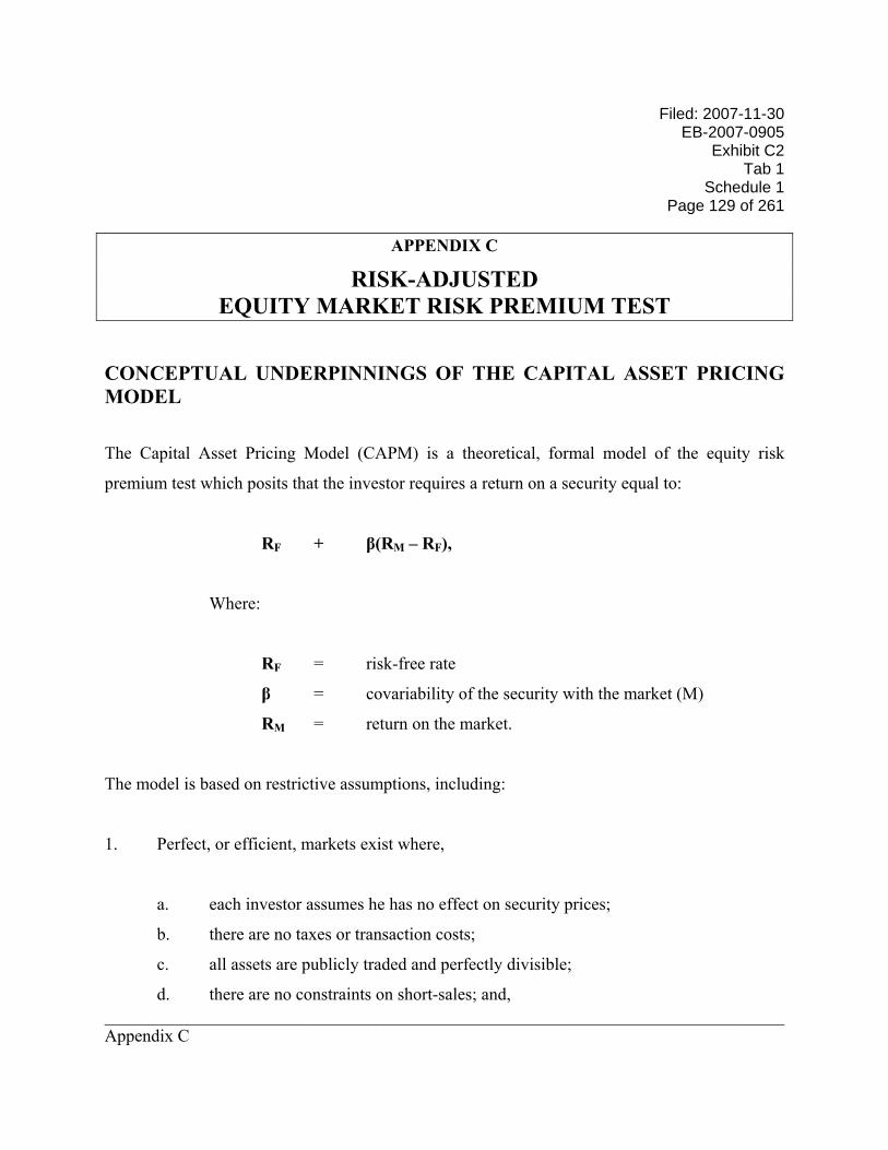
Filed: 2007-11-30 EB-2007-0905
Exhibit C2 Tab 1
Schedule 1 Page 129 of 261
______________________________________________________________________________ Appendix C
APPENDIX C RISK-ADJUSTED
EQUITY MARKET RISK PREMIUM TEST
CONCEPTUAL UNDERPINNINGS OF THE CAPITAL ASSET PRICING MODEL The Capital Asset Pricing Model (CAPM) is a theoretical, formal model of the equity risk
premium test which posits that the investor requires a return on a security equal to:
RF + β(RM – RF),
Where:
RF = risk-free rate
β = covariability of the security with the market (M)
RM = return on the market.
The model is based on restrictive assumptions, including:
1. Perfect, or efficient, markets exist where,
a. each investor assumes he has no effect on security prices;
b. there are no taxes or transaction costs;
c. all assets are publicly traded and perfectly divisible;
d. there are no constraints on short-sales; and,

Filed: 2007-11-30 EB-2007-0905 Exhibit C2 Tab 1 Schedule 1 Page 130 of 261
______________________________________________________________________________ Appendix C
e. the same risk-free rate applies to both borrowing and lending.
2. Investors are identical with respect to their holding period, their expectations and the fact
that all choices are made on the basis of risk and return.
The CAPM relies on the premise that an investor requires compensation for non-diversifiable
risks only. Non-diversifiable risks are those risks that are related to overall market factors (e.g.,
interest rate changes, economic growth). Company-specific risks, according to the CAPM, can
be diversified away by investing in a portfolio of securities whose expected returns are not
perfectly correlated. Therefore, a shareholder requires no compensation to bear company-
specific risks.
In the CAPM, non-diversifiable risk is captured in the beta, which, in principle, is a forward-
looking (expectational) measure of the volatility of a particular stock or portfolio of stocks,
relative to the market. Specifically, the beta is equal to:
Covariance (RE,RM) Variance (RM)
The variance of the market return is intended to capture the uncertainty related to economic
events as they impact the market as a whole. The covariance between the return on a particular
stock and that of the market reflects how responsive the required return on an individual security
is to changes in events that also change the required return on the market.

Filed: 2007-11-30 EB-2007-0905
Exhibit C2 Tab 1
Schedule 1 Page 131 of 261
______________________________________________________________________________ Appendix C
RISK-FREE RATE
1. The theoretical CAPM assumes that the risk-free rate is uncorrelated with the return on
the market. In other words, the assumption is that there is no relationship between the
risk-free rate and the equity market return (i.e., the risk-free rate has a zero beta).
However, the application of the model typically assumes that the return on the market is
highly correlated with the risk-free rate, that is, that the equity market return and the risk-
free rate move in tandem.
2. The theoretical CAPM calls for using a risk-free rate, whereas the typical application of
the model in the regulatory context employs a long-term government bond yield as a
proxy for the risk-free rate. Long-term government bond yields may reflect various
factors that render them problematic as an estimate of the “true” risk-free rate, including:
a. The yield on long-term government bonds reflects the impact of monetary and
fiscal policy; e.g., the potential existence of a scarcity premium. The Canadian
federal government has been in a surplus position for nine years, which has
reduced its financing requirements. However, the demand for long-term
government securities by institutions (e.g., pension funds) that match assets and
liabilities has not declined. The pension funds, which are key purchasers of long-
term government bonds, are typically buy and hold investors, which means that
the government bonds in their portfolios do not trade. Thus, there is the potential
not only for a scarcity premium in prices due to the demand for long-term
government bonds, but also potential illiquidity in the market.
Filed: 2007-11-30 EB-2007-0905 Exhibit C2 Tab 1 Schedule 1 Page 132 of 261
______________________________________________________________________________ Appendix C
b. Yields on long-term government bonds may reflect shifting degrees of investors’
risk aversion; e.g., “flight to quality”. An increase in the equity risk premium
arising from a reduction in bond yields due to a “flight to quality” is not likely to
be captured in the typical application of the CAPM which focuses on a long-term
average market risk premium.
c. Long-term government bond yields are not risk-free; they are subject to interest
rate risk. The size of the equity market risk premium at a given point in time
depends in part on how risky long-term government bond yields are relative to the
overall equity market. The need to capture and measure changes in the risk of the
so-called risk-free security introduces a further complication in the application of
the CAPM.
EQUITY MARKET RISK PREMIUM
1. Equity Risk Premium and Historic Data
The equity market risk premium is typically measured largely by reference to historic
data. Adjustments are then made to capture (a) changes that have occurred in the
underlying markets over time, or (b) perceived differences between what investors
actually achieved and what they may have expected on an ex ante basis. There are a wide
range of views on what constitutes an appropriate period for estimating the historic risk
premium, on what constitutes the appropriate averaging technique, and on whether
various time-specific or country-specific outcomes diminish the reliability of history as a
Filed: 2007-11-30 EB-2007-0905
Exhibit C2 Tab 1
Schedule 1 Page 133 of 261
______________________________________________________________________________ Appendix C
predictor of the future (expected) risk premium. In summary, the link between the
historic and the expected risk premium is subject to considerable judgment.
2. Factors specific to the Canadian historic risk premium data are problematic.
a. The Canadian equity market has undergone significant structural changes over the
periods typically used to measure historic risk premiums. The historic market
returns reflect in considerable measure a resource-based economy. At the end of
1980, no less than 46% of the market value of the TSE 300 was resource-based
stocks.121 By comparison, at the end of 2000, the resource-based percentage of
the S&P/TSX Composite had declined to 18.4%. The influence of technology-
intensive and service-related sectors on the index, in comparison had risen
markedly. In particular, financial services had become a key sector of the equity
composite. Table C-1, which compares the year-end 1980 and 2000 market
weightings of the financial services and technology sectors, highlights the
changes that occurred between 1980 and 2000.
121 As measured by the oil and gas, gold and precious minerals, metals/minerals, and pulp and paper products sectors. Excludes “the conglomerates sector”, which also contained stocks with significant commodity exposure.

Filed: 2007-11-30 EB-2007-0905 Exhibit C2 Tab 1 Schedule 1 Page 134 of 261
______________________________________________________________________________ Appendix C
Table C-1
1980 2000
Biotechnology/ Health Care/ Pharmaceuticals
0.0% 2.8
Information Technology 0.9% 24.1 Telecommunication Services 4.8% 6.5 Media & Entertainment 0.6% 4.1 Financial Services 13.5% 24.1
19.8% 61.1
Source: TSE Review, December 1980 and December 2000.
By the end of August 2007, with the run-up in commodity prices since mid-2004,
(and, to a lesser extent, with the implosion of the information technology sector in
2001), the resource-based sectors (comprised of the Energy sector and the largely
mining-based Materials sector) once again have become a dominant component of
the equity market, accounting for 43.5% of the total market value of the
S&P/TSX Composite, with financial services second. With almost 75% of the
S&P/TSX Composite’s market value in three sectors, the Energy sector at 27% of
the total market value of the Composite, the Financial sector at 31% and Materials
at 17%, the Canadian market has, to some extent, had characteristics of market
sectors, rather than of a diversified portfolio.
By comparison, the U.S. market is significantly more balanced among industry
sectors. A comparison of market weights in Canada and the U.S. of the major
sectors at August 31, 2007 demonstrates the difference.
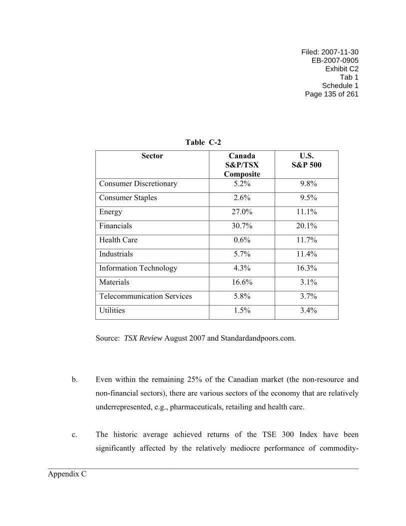
Filed: 2007-11-30 EB-2007-0905
Exhibit C2 Tab 1
Schedule 1 Page 135 of 261
______________________________________________________________________________ Appendix C
Table C-2
Sector Canada S&P/TSX Composite
U.S. S&P 500
Consumer Discretionary 5.2% 9.8%
Consumer Staples 2.6% 9.5%
Energy 27.0% 11.1%
Financials 30.7% 20.1%
Health Care 0.6% 11.7%
Industrials 5.7% 11.4%
Information Technology 4.3% 16.3%
Materials 16.6% 3.1%
Telecommunication Services 5.8% 3.7%
Utilities 1.5% 3.4%
Source: TSX Review August 2007 and Standardandpoors.com.
b. Even within the remaining 25% of the Canadian market (the non-resource and
non-financial sectors), there are various sectors of the economy that are relatively
underrepresented, e.g., pharmaceuticals, retailing and health care.
c. The historic average achieved returns of the TSE 300 Index have been
significantly affected by the relatively mediocre performance of commodity-
Filed: 2007-11-30 EB-2007-0905 Exhibit C2 Tab 1 Schedule 1 Page 136 of 261
______________________________________________________________________________ Appendix C
linked securities over the long-term. From 1956-2003 (the longest period for
which consistent data exist for the individual TSE 300 sub-indices), the average
returns of the commodity-based sectors were exceeded by the returns of virtually
every other sector of the TSE 300.122 Because the long-term returns of the
various sectors are inconsistent with their relative risk, the achieved returns for
the market composite may not accurately reflect what investors had expected.
d. In 2005, the S&P/TSX Composite underwent a significant change with the
inclusion of income trusts. Income trusts, which just five years ago, had a market
capitalization of approximately $20 billion, had a market capitalization of
approximately $189 billion at the end of 2006, accounting for approximately 9%
of the total market value of the TSX. Despite the change to the income tax
treatment of income trusts announced in October 2006, income trusts significantly
outperformed the “conventional” equity markets during the period for which
income trust market data are readily available. The annual total return for the
S&P/TSX Capped Income Trust Index over the 1998-2006 period averaged
16.4%, compared to 9.4% for the S&P/TSX Composite Index. The exclusion of
income trust returns from the S&P/TSX Composite Index prior to 2005 means
that the measured equity returns using the Composite Index understate the actual
equity market returns achieved by Canadian investors.
122 The average (compound, or geometric) returns of the commodity-based sectors were as follows:
Metals/Minerals 7.8% Gold 9.5% Oil and Gas 9.5% Paper/Forest 7.1%
By comparison, the corresponding simple average of the remaining sectors’ returns over the same period was 10.3%.
Filed: 2007-11-30 EB-2007-0905
Exhibit C2 Tab 1
Schedule 1 Page 137 of 261
______________________________________________________________________________ Appendix C
e. The TSE 300 Index has been criticized for its lack of liquidity and for the quality
and size of the stocks it has contained. In a speech in early 2002, Joseph Oliver,
President and CEO of the Investment Dealers Association of Canada stated,
Over the last 25 years, the TSE 300 has steadily declined as a relevant benchmark index. Part of the problem relates to the illiquidity of the smaller component companies and part to the departure of larger companies that were merged or acquired. Over the last two years, 120 Canadian companies have been deleted from the TSE 300.
When a company disappears from a US index due to a merger or acquisition, that doesn’t affect the U.S. market’s liquidity. An ample supply of large cap, liquid U.S. companies can take its place. In Canada, when a company merges or is acquired by another company, it leaves the index and is replaced by a smaller, less liquid Canadian company. We have seen this over the last two years, -- notably in the energy sector. Over the next few years, we are likely to see it in financial services, where further consolidation is inevitable. Over time, Canada’s senior index has become less diversified, with more smaller component companies. As a result, as many as 75 of the TSE 300 will not qualify for inclusion in the new S&P/TSE Composite Index.
When the TSE 300 was overhauled (becoming the S&P/TSX Composite in May
2002), 275 companies were initially included, instead of the previous 300.123 At
December 31, 2005 there were 278 companies in the Composite, including the
recently added income trusts.
f. The performance of the Canadian equity market as the “market portfolio” has
been unduly influenced by a small number of companies. In mid-2000, before the
123 The overhaul of the composite index, which included more stringent criteria for inclusion, did not require that a specific number of companies be included in the index.
Filed: 2007-11-30 EB-2007-0905 Exhibit C2 Tab 1 Schedule 1 Page 138 of 261
______________________________________________________________________________ Appendix C
debacle in Nortel Networks’ stock value, Nortel shares alone accounted for 34.6%
of the total market value of the TSE 300. To put this in perspective, the largest
stock in the S&P 500 at that time (General Electric) accounted for only 4% of the
S&P 500’s total market value. The undue influence of a small number of stocks
requires caution in drawing conclusions from the history of the TSE 300
regarding the forward-looking market risk premium.
g. The returns in the Canadian market have historically been negatively impacted by
the existence of restrictions on the foreign content of assets held in pension plans
and tax deferred savings plans such as Registered Retirement Savings Plans
(RRSPs). In 1957, when tax deferred savings plans were first established, no
more than 10% of the income in pension plans or RRSPs could come from foreign
sources. The Foreign Property Rule was instated in 1971 and limited foreign
content to 10% of the book value of assets in the funds. The limit was raised to
20% in 2% increments between 1990 and 1994.
In 1999, the Investment Funds Institute of Canada (IFIC) estimated that raising
the cap to 20% had increased returns by 1% and that a 30% limit would increase
returns a further 0.5%.124 The limit was raised to 30% in 5% increments between
2000 and 2001. In 2002, the Pension Investment Association of Canada (PIAC)
and the Association of Canadian Pension Management (ACPM) published a
report entitled The Foreign Property Rule: A Cost-Benefit Analysis,125 which
124 Paving the Way for Change to RRSP Foreign Content Rules, Tom Hockin, President and CEO IFIC, January 31, 2000. 125 David Burgess and Joel Fried, The Foreign Property Rule: A Cost-Benefit Analysis, The University of Western Ontario, November 2002.

Filed: 2007-11-30 EB-2007-0905
Exhibit C2 Tab 1
Schedule 1 Page 139 of 261
______________________________________________________________________________ Appendix C
supported the removal of the cap.126 The Globe and Mail reported that the
removal of the foreign content cap is expected to “have the broadest long-term
impact of any personal finance measure in the budget. Global stock markets,
accessible to any investor through global equity mutual funds, have historically
made higher returns than the Canadian market, which only accounts for just over
2 per cent of the world’s stock market value.”127 The Foreign Property Rule was
finally eliminated in August 2005 effective January 1, 2005.
h. The achieved equity market risk premiums in Canada have been squeezed by the
performance of the government bond market. The radical change in Canada’s
fiscal performance over the past decade has contributed to a steady decline in
interest rates and concomitant increases in total bond returns. The prevailing low
level of interest rates relative to the historic total returns on bonds indicates that
the historic returns on long-term Government of Canada bonds overstate likely
future bond returns. Consequently the historic equity risk premium understates
the future risk premium.
126 The IFIC’s report Year 2002 in Review stated,
During the period of 1991-1998, the percentage of sales in equity mutual funds that were comprised of non-domestic equities has hovered around the 41-58% range. This has significantly increased in 1999 and onwards. While performance in the markets is the major factor affecting such an increase, these figures can also be attributed to increases in foreign content limits in registered retirement savings plans as well as increased interest and availability of foreign clone funds.
127 Rob Carrick, Finance: Your Bottom Line, Globeandmail.com, February 23, 2005.
Filed: 2007-11-30 EB-2007-0905 Exhibit C2 Tab 1 Schedule 1 Page 140 of 261
______________________________________________________________________________ Appendix C
3. Use of Arithmetic Averages to Estimate the Equity Market Risk Premium
a. Rationale for the Use of Arithmetic Averages
In Robert F. Bruner, Kenneth M. Eades, Robert S. Harris, and Robert C. Higgins,
“Best Practices in Estimating the Cost of Capital: Survey and Synthesis”,
Financial Practice and Education, Spring/Summer 1998, pp. 13-28, the authors
found that 71% of the texts and tradebooks in their survey supported use of an
arithmetic mean for estimation of the cost of equity. One such textbook, Richard
A. Brealey and Stewart C. Myers, Principles of Corporate Finance, Boston: Irwin
McGraw Hill, 2000 (p. 157), states, “Moral: If the cost of capital is estimated
from historical returns or risk premiums, use arithmetic averages, not compound
annual rates of return.”
The appropriateness of using arithmetic averages, as opposed to geometric
averages, for this purpose is succinctly explained in Ibbotson Associates; Stocks,
Bonds, Bills and Inflation, 1998 Yearbook, pp. 157-159:
The expected equity risk premium should always be calculated using the arithmetic mean. The arithmetic mean is the rate of return which when compounded over multiple periods, gives the mean of the probability distribution of ending wealth values . . . in the investment markets, where returns are described by a probability distribution, the arithmetic mean is the measure that accounts for uncertainty, and is the appropriate one for estimating discount rates and the cost of capital.128
128 An illustration from Ibbotson Associates demonstrating why the arithmetic average is more appropriate than the geometric average for estimating the expected risk premium is presented in Figure C-1.
Filed: 2007-11-30 EB-2007-0905
Exhibit C2 Tab 1
Schedule 1 Page 141 of 261
______________________________________________________________________________ Appendix C
Triumph of the Optimists: 101 Years of Global Investment Returns by Elroy Dimson, Paul Marsh and Mike Staunton, Princeton: Princeton University Press, 2002 (p. 182), stated,
The arithmetic mean of a sequence of different returns is always larger than the geometric mean. To see this, consider equally likely returns of +25 and –20 percent. Their arithmetic mean is 2½ percent, since (25 – 20)/2 = 2½. Their geometric mean is zero, since (1 + 25/100) x (1 – 20/100) – 1 = 0. But which mean is the right one for discounting risky expected future cash flows? For forward-looking decisions, the arithmetic mean is the appropriate measure.
To verify that the arithmetic mean is the correct choice, we can use the 2½ percent required return to value the investment we just described. A $1 stake would offer equal probabilities of receiving back $1.25 or $0.80. To value this, we discount the cash flows at the arithmetic mean rate of 2½ percent. The present values are respectively $1.25/1.025 = $1.22 and $0.80/1.025 = $0.78, each with equal probability, so the value is $1.22 x ½ + $0.80 x ½ = $1.00. If there were a sequence of equally likely returns of +25 and –20 percent, the geometric mean return will eventually converge on zero. The 2½ percent forward-looking arithmetic mean is required to compensate for the year-to-year volatility of returns.
b. Illustration of Why Arithmetic Average Should be Used
In Ibbotson Associates, Stocks, Bonds, Bills and Inflation: Valuation Edition,
2005, the following discussion was included:
To illustrate how the arithmetic mean is more appropriate than the geometric mean in discounting cash flows, suppose the expected return on a stock is 10 percent per year with a standard deviation of 20 percent. Also assume that only two outcomes are possible each year +30 percent and -10 percent (i.e., the mean plus or minus one standard deviation). The probability of occurrence for each outcome is equal. The growth of wealth over a two-year period is illustrated in Graph 5-4.
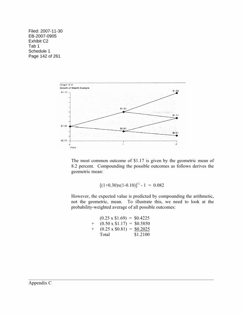
Filed: 2007-11-30 EB-2007-0905 Exhibit C2 Tab 1 Schedule 1 Page 142 of 261
______________________________________________________________________________ Appendix C
The most common outcome of $1.17 is given by the geometric mean of 8.2 percent. Compounding the possible outcomes as follows derives the geometric mean:
[(1+0.30)x(1-0.10)]½ - 1 = 0.082
However, the expected value is predicted by compounding the arithmetic, not the geometric, mean. To illustrate this, we need to look at the probability-weighted average of all possible outcomes:
(0.25 x $1.69) = $0.4225
+ (0.50 x $1.17) = $0.5850 + (0.25 x $0.81) = $0.2025 Total $1.2100
Filed: 2007-11-30 EB-2007-0905
Exhibit C2 Tab 1
Schedule 1 Page 143 of 261
______________________________________________________________________________ Appendix C
Therefore, $1.21 is the probability-weighted expected value. The rate that must be compounded to achieve the terminal value of $1.21 after 2 years is 10 percent, the arithmetic mean.
$1 x (1+0.10)2 = $1.21
The geometric mean, when compounded, results in the median of the distribution:
$1 x (1+0.0.082)2 = $1.17
The arithmetic mean equates the expected future value with the present value; it is therefore the appropriate discount rate.
c. Randomness of Annual Equity Market Risk Premiums
The use of arithmetic averages is premised on the unpredictability of future risk
premiums. The following figures illustrate the uncertainty in the future risk
premiums by reference to the historic annual risk premiums. The figures for both
Canada and the U.S. suggest that each year’s actual risk premium has been
random, that is, not serially correlated with the preceding year’s risk premium.129
129 A test for serial correlation between the year-to-year equity risk premiums shows that the serial correlation between the current year’s risk premium and that of the prior year for the period 1947-2006 is 0.06 for Canada and −0.05 for the U.S. If the current year’s risk premium were predictable based on the prior year’s risk premium, the serial correlation would be close to positive or negative 1.0.
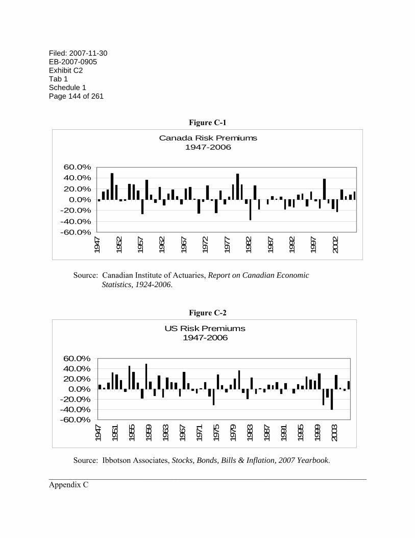
Filed: 2007-11-30 EB-2007-0905 Exhibit C2 Tab 1 Schedule 1 Page 144 of 261
______________________________________________________________________________ Appendix C
Figure C-1
Canada Risk Premiums1947-2006
-60.0%-40.0%-20.0%
0.0%20.0%40.0%60.0%
1947
1952
1957
1962
1967
1972
1977
1982
1987
1992
1997
2002
Source: Canadian Institute of Actuaries, Report on Canadian Economic Statistics, 1924-2006.
Figure C-2
US Risk Premiums1947-2006
-60.0%-40.0%-20.0%
0.0%20.0%40.0%60.0%
1947
1951
1955
1959
1963
1967
1971
1975
1979
1983
1987
1991
1995
1999
2003
Source: Ibbotson Associates, Stocks, Bonds, Bills & Inflation, 2007 Yearbook.
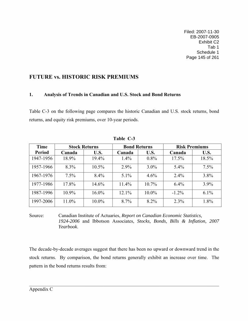
Filed: 2007-11-30 EB-2007-0905
Exhibit C2 Tab 1
Schedule 1 Page 145 of 261
______________________________________________________________________________ Appendix C
FUTURE vs. HISTORIC RISK PREMIUMS
1. Analysis of Trends in Canadian and U.S. Stock and Bond Returns
Table C-3 on the following page compares the historic Canadian and U.S. stock returns, bond
returns, and equity risk premiums, over 10-year periods.
Table C-3
Stock Returns Bond Returns Risk Premiums Time Period Canada U.S. Canada U.S. Canada U.S.
1947-1956 18.9% 19.4% 1.4% 0.8% 17.5% 18.5%
1957-1966 8.3% 10.5% 2.9% 3.0% 5.4% 7.5%
1967-1976 7.5% 8.4% 5.1% 4.6% 2.4% 3.8%
1977-1986 17.8% 14.6% 11.4% 10.7% 6.4% 3.9%
1987-1996 10.9% 16.0% 12.1% 10.0% -1.2% 6.1%
1997-2006 11.0% 10.0% 8.7% 8.2% 2.3% 1.8%
Source: Canadian Institute of Actuaries, Report on Canadian Economic Statistics,
1924-2006 and Ibbotson Associates, Stocks, Bonds, Bills & Inflation, 2007 Yearbook.
The decade-by-decade averages suggest that there has been no upward or downward trend in the
stock returns. By comparison, the bond returns generally exhibit an increase over time. The
pattern in the bond returns results from:
Filed: 2007-11-30 EB-2007-0905 Exhibit C2 Tab 1 Schedule 1 Page 146 of 261
______________________________________________________________________________ Appendix C
♦ low bond returns in the 1950s-1970s, as rising interest rates produced capital losses on
bonds;
♦ high bond returns in the 1980s, corresponding to the high rates of inflation, which pushed
up bond yields; and,
♦ high bond returns in the 1990s and first half of the 2000s, reflecting the decline in interest
rates and resulting capital appreciation of bonds, leading to total returns well in excess of
the yields.130
A similar conclusion regarding trends in the risk premium can be drawn from an analysis of
rolling and cumulative averages of Canadian and U.S. stock and bond returns. The following
averages were calculated for this analysis:
♦ Twenty-five year rolling arithmetic averages of Canadian and U.S. equity and long-term
government bond returns (1947-2006).
♦ A series of cumulative average equity and bond returns for Canada and the U.S. The first
average starts in 1947, covering 25 years (1947-1971). The second average incorporates
26 years, etc. The final average encompasses the full 1947-2006 period.
♦ A second series of cumulative average returns, where the first average includes the most
recent 25 year period (1982-2006); each subsequent average includes an additional prior
year.
130 The bond yield is, in fact, an estimate of the expected return.
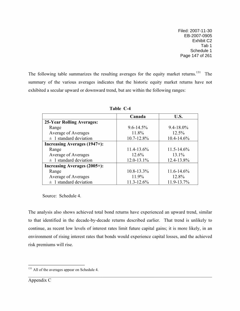
Filed: 2007-11-30 EB-2007-0905
Exhibit C2 Tab 1
Schedule 1 Page 147 of 261
______________________________________________________________________________ Appendix C
The following table summarizes the resulting averages for the equity market returns.131 The
summary of the various averages indicates that the historic equity market returns have not
exhibited a secular upward or downward trend, but are within the following ranges:
Table C-4
Canada U.S. 25-Year Rolling Averages: Range Average of Averages ± 1 standard deviation
9.6-14.5%
11.8% 10.7-12.8%
9.4-18.0%
12.5% 10.4-14.6%
Increasing Averages (1947+): Range Average of Averages ± 1 standard deviation
11.4-13.6%
12.6% 12.0-13.1%
11.5-14.6%
13.1% 12.4-13.8%
Increasing Averages (2005+): Range Average of Averages ± 1 standard deviation
10.8-13.3%
11.9% 11.3-12.6%
11.6-14.6%
12.8% 11.9-13.7%
Source: Schedule 4.
The analysis also shows achieved total bond returns have experienced an upward trend, similar
to that identified in the decade-by-decade returns described earlier. That trend is unlikely to
continue, as recent low levels of interest rates limit future capital gains; it is more likely, in an
environment of rising interest rates that bonds would experience capital losses, and the achieved
risk premiums will rise.
131 All of the averages appear on Schedule 4.
Filed: 2007-11-30 EB-2007-0905 Exhibit C2 Tab 1 Schedule 1 Page 148 of 261
______________________________________________________________________________ Appendix C
Given the absence of any upward or downward trend in the historic equity market returns, a
reasonable expected value of the future equity market return is a range of 11.5-12.5%, based on
both the Canadian and U.S. equity market returns. Based on the 2008 forecast for long Canada
bond yields of 5.0%132, and an expected equity market return of 11.5-12.5%, the indicated
market risk premium would be in the range of 6.5-7.5%, or approximately 7.0%. Based on the
longer-term forecast for long Canada bond yields of approximately 5.25%,133 the indicated
market risk premium is 6.25-7.25%.
2. Trends in Price/Earnings Ratios
Several studies of historic and equity risk premiums conclude that past equity markets are
unsustainable, since they were achieved through an increase in price/earnings ratios that cannot
be perpetuated.
With respect to the U.S. equity market, the preponderance of the increase in price/earnings ratios
occurred during the 1990s. The P/E ratio134 of the S&P 500 averaged 14 times from 1926-1989,
with no discernible upward trend.135 From 14.7 in 1989, the P/E ratio rose to a high of 32.3 in
1998, and averaged 23 from 1990-2000. At the height of the equity market (1998 to mid-2000),
frequently described as a “speculative bubble”, investors believed the only risk they faced was
not being in the equity market. In mid-2000, the bubble burst, as the U.S. economy began to lose
steam. The events of September 11, 2001, the threat of war, the loss of credibility on Wall
132 Based on the August 2007 Consensus Forecast. 133 The 2008 forecast is, as previously noted, 5.0%. Consensus Economics, Consensus Forecasts, April 2007 anticipates the 10-year Canada bond yield to average approximately 5.0% from 2009 to 2017. Adding a spread of approximately 10 (as of August 2007) to 30 (historic average) basis points to the 5.0% forecast results in a 30-year Canada bond yield forecast of close to 5.25%. 134 Coincident price and earnings. 135 The average from 1947-1989 was 13.3 times.
Filed: 2007-11-30 EB-2007-0905
Exhibit C2 Tab 1
Schedule 1 Page 149 of 261
______________________________________________________________________________ Appendix C
Street, accounting misrepresentations and outright fraud, led to a loss of confidence in the market
and a sense of pessimism about the equity market. These events led to a heightened appreciation
of the inherent risk of investing in the equity market, all of which translated into a “bearish”
outlook for the U.S. equity market and sent retail investors to the sidelines.136 Nevertheless, the
P/E ratio for the S&P 500 remains above the average for 1947-1989, but within the historic
range.137
To assess the impact of rising P/E ratios on achieved returns, I analyzed the equity returns of the
S&P 500 achieved between 1947 and 1990, that is, prior to the observed upward trend in P/E
ratios. The analysis indicates that the achieved equity returns for the S&P 500 averaged 12.3%
(geometric average) to 13.5% (arithmetic average) from 1947-1989. The corresponding returns
from 1947-2006 were 11.9% (geometric average) to 13.2% (arithmetic average). Hence, despite
the increase in P/E ratios experienced during the 1990s, the average equity market returns were
actually lower over the entire 1947-2006 period than over the 1947-1989 period. Stated
differently, the increase in P/E ratios during the 1990s has not resulted in a higher and
unsustainable level of equity market returns. Consequently, based on history, an expected value
for the U.S. equity market return equal to the historic levels of 12.0-13.0% is not unreasonable.
Relative to the consensus forecast yield for 30-year Treasury bonds for 2007 and for the longer
term of approximately 5.3%,138 the risk premium would be approximately 6.75-7.75%.
My review of Canadian equity returns over the same period indicates similar results. The 1947-
1989 returns for the Canadian equity market were 11.9% (geometric average) to 13.1% 136 Lowered expectations for the equity market have led investors to focus elsewhere for superior risk/reward opportunities, e.g., real estate, and private equity, suggesting the possibility that recent expectations for the public equity market may be out-of-line with return requirements. Investors’ experiences during the equity market “bust” have been a key factor in explaining the recent burgeoning of the income trust market in Canada. 137 At the end of August 2007, the S&P 500 P/E ratio was 17.3. 138 For 2008-2017; Blue Chip Financial Forecasts, August 1, 2007 and June 1, 2007.
Filed: 2007-11-30 EB-2007-0905 Exhibit C2 Tab 1 Schedule 1 Page 150 of 261
______________________________________________________________________________ Appendix C
(arithmetic average), very similar to the U.S. returns, and higher than the average of the 1947-
2006 returns. In relation to the 2008 and long-term forecasts of the 30-year Canada bond yield,
5.0% and 5.25% respectively, and an expected value of the Canadian equity market returns in the
range of 12.0-13.0%, the expected value for the equity risk premium would be in the range of
approximately 7.0-7.75%.
The analysis of stock and bond returns in Canada and the U.S. over the 1947-2006 period reveals
no upward or downward trend in market equity returns. Nevertheless, the achieved risk
premiums have declined. The arithmetic average achieved risk premium in Canada from 1947-
1989 was 7.6%; in the U.S., it was 8.5%. By comparison, the corresponding 1947-2006 risk
premiums were 5.5% and 6.9% respectively. An analysis of the data shows that high bond
returns over the period 1990-2006 are the principal reason for the decline in experienced risk
premiums, not a downward trend in stock returns. The average bond return from 1990-2006 was
10.6%, compared to the corresponding average yield on long-term Canada bonds of 6.8%.
Over the entire 1947-2006 period, the average return (income plus capital appreciation) on long
Canada bonds was approximately 7.0%. With interest rates currently at historically low levels
(approximately 4.5% at the end of August 2007), and more likely to increase rather than decrease
further, the 1947-2006 average bond return of approximately 7.0% overstates the forward-
looking expectation of bond returns, as embedded in both current yields and long-term forecasts.
The current low level of long-Canada yields limits the possibility of future capital gains, which
arise from a decline in interest rates. Thus, a reasonable expected value of the long Canada bond
return is the forecast long Canada yield, rather than the historic average.
Filed: 2007-11-30 EB-2007-0905
Exhibit C2 Tab 1
Schedule 1 Page 151 of 261
______________________________________________________________________________ Appendix C
RELATIVE RISK ADJUSTMENT
1. Beta
Impediments to reliance on beta as the sole relative risk measure, as the CAPM indicates,
include:
a. The assumption that all risk for which investors require compensation can be
captured and expressed in a single risk variable;
b. The only risk for which investors expect compensation is non-diversifiable equity
market risk; no other risk is considered (and priced) by investors; and,
c. The assumption that the observed calculated betas (which are simply a calculation
of how closely a stock’s or portfolio’s price changes have mirrored those of the
overall equity market)139 are a good measure of the relative return requirement.
d. Use of beta as the relative risk adjustment allows for the conclusion that the cost
of equity capital for a firm can be lower than the risk-free rate, since stocks that
have moved counter to the rest of the equity market could be expected to have
139 The beta is equal to: Covariance (RE,RM) Variance (RM) Betas are typically calculated by reference to historical relative volatility using simple regression analysis of the change in the market portfolio return and the corresponding change in an individual stock or portfolio of stock returns.
Filed: 2007-11-30 EB-2007-0905 Exhibit C2 Tab 1 Schedule 1 Page 152 of 261
______________________________________________________________________________ Appendix C
betas that are negative. Gold stocks, for example, which are regarded as a
quintessential counter-cyclical investment, could reasonably be expected to
exhibit negative betas. In that case, the CAPM would posit that the cost of equity
capital for a gold mining firm would be less than the risk-free rate, despite the fact
that, on a total risk basis, the company’s stock could be very volatile.
The body of evidence on CAPM leads to the conclusion that, while betas do
measure relative volatility, the proportionate relationship between beta and return
posited by the CAPM has not been established. A summary of various studies,
published in a guide for practitioners, concluded,
Empirical tests of the CAPM have, in retrospect, produced results that are often at odds with the theory itself. Much of the failure to find empirical support for the CAPM is due to our lack of ex ante, expectational data. This, combined with our inability to observe or properly measure the return on the true, complete, market portfolio, has contributed to the body of conflicting evidence about the validity of the CAPM. It is also possible that the CAPM does not describe investors’ behavior in the marketplace.
Theoretically and empirically, one of the most troubling problems for academics and money managers has been that the CAPM’s single source of risk is the market. They believe that the market is not the only factor that is important in determining the return an asset is expected to earn. (Diana R. Harrington, Modern Portfolio Theory, The Capital Asset Pricing Model & Arbitrage Pricing Theory: A User’s Guide, Second Edition, Prentice-Hall, Inc., 1987, page 188.)
Fama and French in “The CAPM: Theory and Evidence”, Journal of Economic
Perspectives, Volume 18, Number 3 (Summer 2004), pp. 25-26:
Filed: 2007-11-30 EB-2007-0905
Exhibit C2 Tab 1
Schedule 1 Page 153 of 261
______________________________________________________________________________ Appendix C
The attraction of the CAPM is that it offers powerful and intuitively pleasing predictions about how to measure risk and the relation between expected return and risk. Unfortunately, the empirical record of the model is poor – poor enough to invalidate the way it is used in applications. The CAPM’s empirical problems may reflect theoretical failings, the result of many simplifying assumptions. But they may also be caused by difficulties in implementing valid tests of the model. For example, the CAPM says that the risk of a stock should be measured relative to a comprehensive ‘market portfolio’ that in principle can include not just traded financial assets, but also consumer durables, real estate and human capital. Even if we take a narrow view of the model and limit its purview to traded financial assets, is it legitimate to limit further the market portfolio to U.S. common stocks (a typical choice), or should the market be expanded to include bonds, and other financial assets, perhaps around the world? In the end, we argue that whether the model’s problems reflect weaknesses in the theory or in its empirical implementation, the failure of the CAPM in empirical tests implies that most applications of the model are invalid.
Fama and French have developed an alternative model which incorporates two
additional explanatory factors in an attempt to overcome the problems inherent in
the single variable CAPM.140
To quote Burton Malkiel in A Random Walk Down Wall Street, New York: W. W.
Norton & Co., 2003:
Beta, the risk measure from the capital-asset pricing model, looks nice on the surface. It is a simple, easy-to-understand measure of market sensitivity. Alas, beta also has its warts. The actual relationship between beta and rate of return has not corresponded to the relationship predicted in theory during long periods of the twentieth century. Moreover, betas for individual stocks are not stable from period to period, and they are
140 The additional factors are size and book to market.

Filed: 2007-11-30 EB-2007-0905 Exhibit C2 Tab 1 Schedule 1 Page 154 of 261
______________________________________________________________________________ Appendix C
very sensitive to the particular market proxy against which they are measured.
I have argued here that no single measure is likely to capture adequately the variety of systematic risk influences on individual stocks and portfolios. Returns are probably sensitive to general market swings, to changes in interest and inflation rates, to changes in national income, and, undoubtedly, to other economic factors such as exchange rates. And if the best single risk estimate were to be chosen, the traditional beta measure is unlikely to be everyone’s first choice. The mystical perfect risk measure is still beyond our grasp. (page 240)
One of the key developers of the Arbitrage Pricing Model, Dr. Stephen Ross, has
stated,
Beta is not very useful for determining the expected return on a stock, and it actually has nothing to say about the CAPM. For many years, we have been under the illusion that the CAPM is the same as finding that beta and expected returns are related to each other. That is true as a theoretical and philosophical tautology, but pragmatically, they are miles apart.141
2. Relationship between Beta and Return in the Canadian Equity Market
To test the actual relationship between beta and return in a Canadian context, the betas (using
monthly total return data) were calculated for various periods for each of the 15 major sub-
indices of the “old” TSE 300 as were the corresponding actual geometric average total returns.
Simple regressions of the betas on the achieved market returns were then conducted to determine
if there was indeed the expected positive relationship. The regressions covered (a) 1956-2003,
the longest period for which data for the TSE 300 and its sub-index components are available; 141 Dr. Stephen A. Ross, “Is Beta Useful?” The CAPM Controversy: Policy and Strategy Implications for Investment Management, AIMR, 1993.
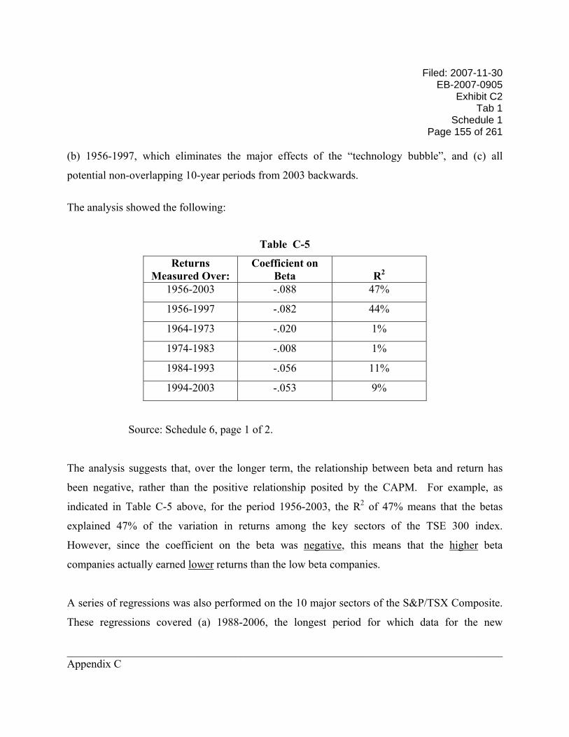
Filed: 2007-11-30 EB-2007-0905
Exhibit C2 Tab 1
Schedule 1 Page 155 of 261
______________________________________________________________________________ Appendix C
(b) 1956-1997, which eliminates the major effects of the “technology bubble”, and (c) all
potential non-overlapping 10-year periods from 2003 backwards.
The analysis showed the following:
Table C-5
Returns Measured Over:
Coefficient on Beta
R2
1956-2003 -.088 47%
1956-1997 -.082 44%
1964-1973 -.020 1%
1974-1983 -.008 1%
1984-1993 -.056 11%
1994-2003 -.053 9%
Source: Schedule 6, page 1 of 2.
The analysis suggests that, over the longer term, the relationship between beta and return has
been negative, rather than the positive relationship posited by the CAPM. For example, as
indicated in Table C-5 above, for the period 1956-2003, the R2 of 47% means that the betas
explained 47% of the variation in returns among the key sectors of the TSE 300 index.
However, since the coefficient on the beta was negative, this means that the higher beta
companies actually earned lower returns than the low beta companies.
A series of regressions was also performed on the 10 major sectors of the S&P/TSX Composite.
These regressions covered (a) 1988-2006, the longest period for which data for the new
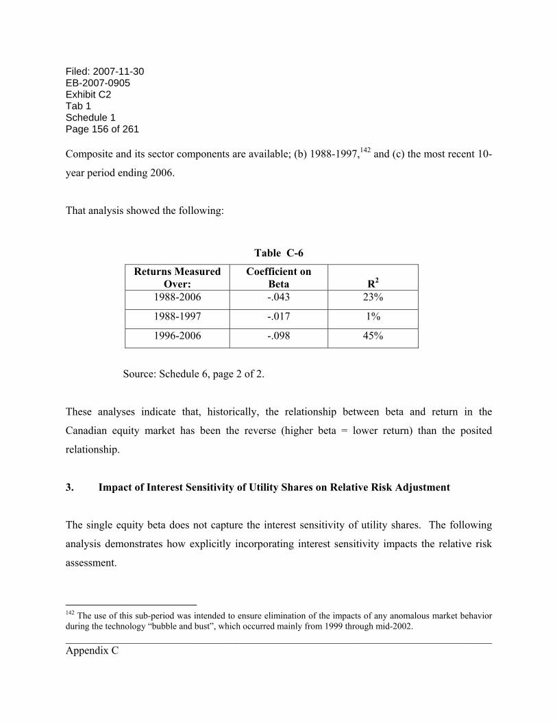
Filed: 2007-11-30 EB-2007-0905 Exhibit C2 Tab 1 Schedule 1 Page 156 of 261
______________________________________________________________________________ Appendix C
Composite and its sector components are available; (b) 1988-1997,142 and (c) the most recent 10-
year period ending 2006.
That analysis showed the following:
Table C-6
Returns Measured Over:
Coefficient on Beta
R2
1988-2006 -.043 23%
1988-1997 -.017 1%
1996-2006 -.098 45%
Source: Schedule 6, page 2 of 2.
These analyses indicate that, historically, the relationship between beta and return in the
Canadian equity market has been the reverse (higher beta = lower return) than the posited
relationship.
3. Impact of Interest Sensitivity of Utility Shares on Relative Risk Adjustment
The single equity beta does not capture the interest sensitivity of utility shares. The following
analysis demonstrates how explicitly incorporating interest sensitivity impacts the relative risk
assessment.
142 The use of this sub-period was intended to ensure elimination of the impacts of any anomalous market behavior during the technology “bubble and bust”, which occurred mainly from 1999 through mid-2002.
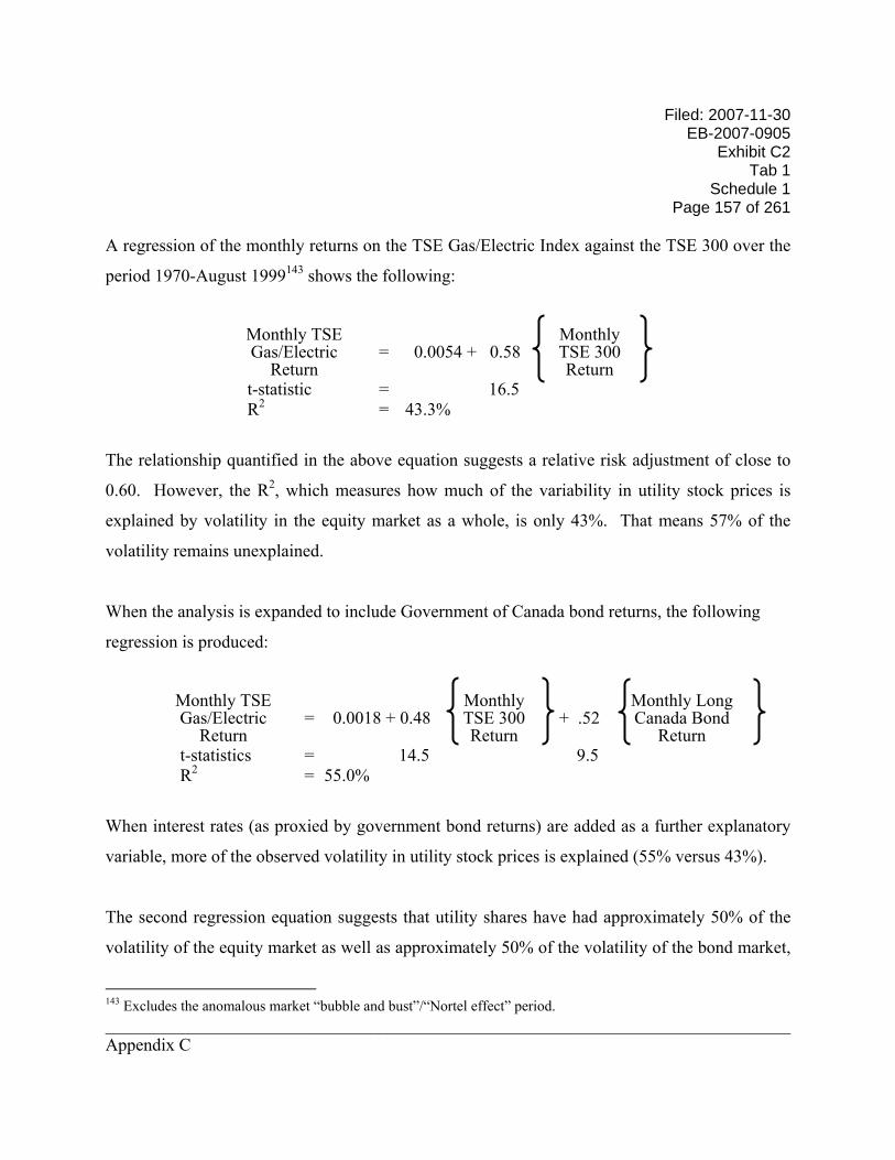
Filed: 2007-11-30 EB-2007-0905
Exhibit C2 Tab 1
Schedule 1 Page 157 of 261
______________________________________________________________________________ Appendix C
A regression of the monthly returns on the TSE Gas/Electric Index against the TSE 300 over the
period 1970-August 1999143 shows the following:
Monthly TSE Gas/Electric
Return
=
0.0054 + 0.58
Monthly TSE 300 Return
t-statistic = 16.5 R2 = 43.3%
The relationship quantified in the above equation suggests a relative risk adjustment of close to
0.60. However, the R2, which measures how much of the variability in utility stock prices is
explained by volatility in the equity market as a whole, is only 43%. That means 57% of the
volatility remains unexplained.
When the analysis is expanded to include Government of Canada bond returns, the following
regression is produced:
Monthly TSE Gas/Electric
Return
=
0.0018 + 0.48
Monthly TSE 300 Return
+ .52
Monthly Long Canada Bond
Return t-statistics = 14.5 9.5 R2 = 55.0%
When interest rates (as proxied by government bond returns) are added as a further explanatory
variable, more of the observed volatility in utility stock prices is explained (55% versus 43%).
The second regression equation suggests that utility shares have had approximately 50% of the
volatility of the equity market as well as approximately 50% of the volatility of the bond market,
143 Excludes the anomalous market “bubble and bust”/“Nortel effect” period.
Filed: 2007-11-30 EB-2007-0905 Exhibit C2 Tab 1 Schedule 1 Page 158 of 261
______________________________________________________________________________ Appendix C
consistent with utility common stocks’ interest sensitivity. Using an expected equity market
return of 11.5%, and a long Canada bond return equal to the 2008 forecast 30-year Canada yield
of 5.0%, the equation indicates an expected utility return of 10.4%. When the 10.4% utility
return is expressed as an equity risk premium relative to the 5.0% long Canada yield, the
indicated relative risk adjustment is close to 83%.144
144
%0.5%5.11%0.5%4.10
−− = .83
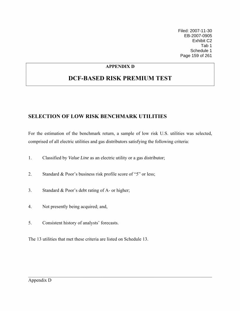
Filed: 2007-11-30 EB-2007-0905
Exhibit C2 Tab 1
Schedule 1 Page 159 of 261
______________________________________________________________________________ Appendix D
APPENDIX D
DCF-BASED RISK PREMIUM TEST
SELECTION OF LOW RISK BENCHMARK UTILITIES
For the estimation of the benchmark return, a sample of low risk U.S. utilities was selected,
comprised of all electric utilities and gas distributors satisfying the following criteria:
1. Classified by Value Line as an electric utility or a gas distributor;
2. Standard & Poor’s business risk profile score of “5” or less;
3. Standard & Poor’s debt rating of A- or higher;
4. Not presently being acquired; and,
5. Consistent history of analysts’ forecasts.
The 13 utilities that met these criteria are listed on Schedule 13.
Filed: 2007-11-30 EB-2007-0905 Exhibit C2 Tab 1 Schedule 1 Page 160 of 261
______________________________________________________________________________ Appendix D
CONSTRUCTION OF THE DCF-BASED EQUITY RISK PREMIUM TEST
The constant growth DCF model was used to construct a monthly series of expected utility
returns for each of the 13 utilities in the sample over the period 1993-2007 (2nd Qtr).145 The
monthly DCF cost for each utility was estimated as the sum of the utilities’ I/B/E/S mean
earnings growth forecast (published monthly) (g) and the corresponding expected monthly
dividend yield (DYe). The dividend yield (DY) was calculated as the most recent quarterly
dividend paid, annualized, divided by the monthly closing price. The expected dividend yield
was then calculated by adjusting the monthly dividend yield for the I/B/E/S median earnings
growth forecast (DYe=DY*(1+g)). The individual utilities’ monthly DCF estimates (DYe + g)
were then averaged to produce a time series of monthly DCF estimates (DCFs) for the sample.
The monthly equity risk premium (ERP) for the sample was calculated by subtracting the
corresponding 30-year Treasury yield (TY) from the average DCF cost of equity (ERPs=DCFs–
TY) (Schedule 12). The monthly sample average ERPs were used to estimate the regression
equations found in Chapter III.C.b.4 of the testimony.
145 Subsequent to Open Access for natural gas transmission implemented via FERC Order 636.
Filed: 2007-11-30 EB-2007-0905
Exhibit C2 Tab 1
Schedule 1 Page 161 of 261
______________________________________________________________________________ Appendix E
APPENDIX E
DISCOUNTED CASH FLOW TEST
DCF MODELS
Constant Growth Model
The constant growth model rests on the assumption that investors expect cash flows to grow at a
constant rate throughout the life of the stock. The assumption that investors expect a stock to
grow at a constant rate over the long-term is most applicable to stocks in mature industries.
Growth rates in these industries will vary from year to year and over the business cycle, but will
tend to deviate around a long-term expected value. As a pragmatic matter, the application of a
constant growth model is compatible with the likelihood that investors do not forecast beyond
five years. Hence, in that context the current market price and dividend yield would not
explicitly anticipate any changes in the outlook for growth.
The constant growth model is expressed as follows:
Cost of Equity (k) = D1 + g,
Po
where, D1 = next expected dividend146 Po = current price g = constant growth rate
146Alternatively expressed as Do (1 + g), where Do is the most recently paid dividend.
Filed: 2007-11-30 EB-2007-0905 Exhibit C2 Tab 1 Schedule 1 Page 162 of 261
______________________________________________________________________________ Appendix E
This model, as set forth above, reflects a simplification of reality. First, it is based on the notion
that investors expect all cash flows to be derived through dividends. Second, the underlying
premise is that dividends, earnings, and price all grow at the same rate. However, it is likely
that, in the near-term, investors expect growth in dividends to be lower than growth in earnings.
The model can be adapted to account for the potential disparity between earnings and dividend
growth by recognizing that all investor returns must ultimately come from earnings. Hence,
focusing on investor expectations of earnings growth will encompass all of the sources of
investor returns (e.g., dividends and retained earnings).
Two-Stage Model
The two-stage model is based on the premise that investors expect the growth rate for the utilities
to be equal to the company-specific growth rates for the near-term (Stage 1 Growth), but, in the
longer-term (from Year 6 onward) to migrate to the expected long-run rate of growth in the
economy (GDP Growth). All industries go through various stages in their life cycle. Utilities
are considered to be the quintessential mature industry. Mature industries are those whose
growth parallels that of the overall economy.
The use of forecast GDP growth as the long-term growth component is a widely utilized
approach. For example, the Merrill Lynch discounted cash flow model for valuation utilizes
nominal GDP growth as a proxy for long-term growth expectations. The Federal Energy
Regulatory Commission relies on GDP growth to estimate expected long-term nominal GDP
growth in its standard DCF models for gas and oil pipelines.
Filed: 2007-11-30 EB-2007-0905
Exhibit C2 Tab 1
Schedule 1 Page 163 of 261
______________________________________________________________________________ Appendix E
Using the two-stage DCF model, the DCF cost of equity is estimated as the internal rate of return
that causes the price of the stock to equal the present value of all future cash flows to the
investor.
The cash flow per share in Year 1 is equal to:
Last Paid Annualized Dividend x (1 + Stage 1 Growth)
For Years 2 through 5, cash flow is defined as:
Cash Flow t-1 x (1 + Stage 1 Growth)
Cash flows from Year 6 onward are estimated as:
Cash Flow t-1 x (1 + GDP Growth)
SELECTION OF PROXY BENCHMARK UTILITIES
The same sample of benchmark utilities was used as for the DCF-based risk premium test. The
selection criteria for these low risk utilities are described in Appendix D.
INVESTOR GROWTH EXPECTATIONS
The application of the constant growth model relies principally on the consensus of investment
analysts’ forecasts of long-term earnings growth compiled by I/B/E/S. The application of the
two-stage model relies upon the I/B/E/S consensus earnings forecasts as the estimate of investor
Filed: 2007-11-30 EB-2007-0905 Exhibit C2 Tab 1 Schedule 1 Page 164 of 261
______________________________________________________________________________ Appendix E
growth expectations during Stage 1. The expected nominal long-run rate of growth in the
economy (GDP) is based on the consensus of economists’ long-term forecasts (published twice
annually) found in Blue Chip Economic Indicators (March 10, 2007). The consensus forecast
rate of growth in the long-term (2009-2018) is 5.1%.
Empirical studies that conclude that investment analysts’ growth forecasts serve as a better
surrogate for investors expectations than historic growth rates include: Lawrence D. Brown and
Michael S. Rozeff, “The Superiority of Analyst Forecasts as Measures of Expectations: Evidence
from Earnings”, The Journal of Finance, Vol. XXXIII, No. 1, March 1978; Dov Fried and Dan
Givoly, “Financial Analysts Forecasts of Earnings, A Better Surrogate for Market Expectations”,
Journal of Accounting and Economics, Vol. 4 (1982); R. Charles Moyer, Robert E. Chatfield,
Gary D. Kelley, “The Accuracy of Long-Term Earnings Forecasts in the Electric Utility
Industry”, International Journal of Forecasting Vol. I (1985); Robert S. Harris, “Using Analysts’
Growth Forecasts to Estimate Shareholder Required Rates of Return”, Financial Management,
Spring 1986, and, James H. Vander Weide and William T. Carleton, “Investor Growth
Expectations: Analysts vs. History”, The Journal of Portfolio Management, Spring 1988; David
Gordon, Myron Gordon and Lawrence Gould, “Choice Among Methods of Estimating Share
Yield,” The Journal of Portfolio Management, Spring 1989.
The Vander Weide and Carleton study cited
found overwhelming evidence that the consensus analysts’ forecast of future growth is superior to historically oriented growth measures in predicting the firm’s stock price [and that these results] also are consistent with the hypothesis that investors use analysts’ forecasts, rather than historically oriented growth calculations, in making stock buy-and-sell decisions.
Filed: 2007-11-30 EB-2007-0905
Exhibit C2 Tab 1
Schedule 1 Page 165 of 261
______________________________________________________________________________ Appendix E
The Gordon, Gordon and Gould study concluded, …the superior performance by KFRG [forecasts of [earnings] growth by securities
analysts] should come as no surprise. All four estimates [securities analysts’ forecasts plus past growth in earnings and dividends and historic retention growth rates] rely upon past data, but in the case of KFRG a larger body of past data is used, filtered through a group of security analysts who adjust for abnormalities that are not considered relevant for future growth.
In the application of the DCF test, the reliability of the earnings growth forecasts as a measure of
investor expectations has been questioned by some Canadian regulators. The issue of reliability
arises because of the documented optimism of analysts’ forecasts historically. However, as long
as investors have believed the forecasts, and have priced the securities accordingly, the resulting
DCF costs of equity are an unbiased estimate of investors’ expected returns. That proposition
can be tested indirectly. For the sample of low risk utilities used in the DCF test (as well as the
DCF-based equity risk premium test to estimate the benchmark return on equity), the average
expected long-term growth rate, as estimated using analysts’ forecasts, for the entire 1993-2007
(2nd Qtr) period of analysis was 4.7%. That growth rate is lower than the expected long-term
nominal growth in the economy as a whole over the same period.147 An expected growth rate
that is close to that of the economy as a whole would not be out-of-line with the level of growth
investors could reasonably expect in the relatively mature utility industries over the longer-term.
147 The average expected long-term nominal rate of growth in the U.S. economy, based on consensus forecasts (Blue Chip Economic Indicators, March editions, 1993-2007), has been 5.3% over the same period covered by the DCF-based equity risk premium test.
Filed: 2007-11-30 EB-2007-0905 Exhibit C2 Tab 1 Schedule 1 Page 166 of 261
______________________________________________________________________________ Appendix E
APPLICATION OF THE DCF MODELS
Constant Growth Model
The constant growth DCF model was applied to the sample of U.S. low risk gas and electric
utilities using the following inputs to calculate the dividend yield:
1. the most recent annualized dividend paid as of July 31, 2007 as Do; and,
2. the average of the daily close prices for the period July 16 to August 15, 2007 as Po.
For the expected growth rates, the July 2007 I/B/E/S consensus (mean) earnings growth forecasts
were used to estimate “g” in the growth component for each utility and to adjust the current
dividend yield to the expected dividend yield. The DCF estimates of the cost of equity for the
benchmark sample based on the constant growth model were approximately 9.3% (See Schedule
14).
Two-Stage Model
The two-stage model relies on the I/B/E/S consensus of analysts’ earnings forecasts for the first
five years (Stage 1), and forecast growth in the economy thereafter (Stage 2). The consensus
long-run (2009-2018) expected nominal rate of growth in GDP, as noted above, is 5.1%.
Filed: 2007-11-30 EB-2007-0905
Exhibit C2 Tab 1
Schedule 1 Page 167 of 261
______________________________________________________________________________ Appendix E
The two-stage DCF model estimates of the cost of equity for the benchmark low risk U.S. utility
sample (Schedule 15) are as follows:
Mean 9.4%
Median 9.5%
Results of the Constant Growth and Two-Stage Models
The results of the two models indicate a required “bare-bones” return on equity of approximately
9.25% (constant growth model) to 9.5% (two-stage model).
Filed: 2007-11-30 EB-2007-0905 Exhibit C2 Tab 1 Schedule 1 Page 168 of 261
______________________________________________________________________________ Appendix F
APPENDIX F COMPARABLE EARNINGS TEST
SELECTION OF CANADIAN INDUSTRIALS
The selection process starts with the recognition that industrials generally are exposed to higher
business risk, but lower financial risk, than a benchmark Canadian utility. The selection of
industrials focuses on total investment risk, i.e., the combined business and financial risks. The
comparable earnings test is based on the premise that industrials' higher business risks are offset
by a more conservative capital structure, i.e., higher equity ratios, thus permitting selection of
industrial samples of reasonably comparable investment risk to a benchmark Canadian utility.
As a point of departure, the selection was limited to industries that are characterized by relatively
stable demand characteristics, as well as consistent dividend payments and relatively low
earnings and share price volatility. The initial universe consisted of all firms on the TSX in
Global Industry Classification Standard (GICS) sectors 20-30. The sectors represented by the
GICS codes in this range are: Industrials, Consumer Discretionary and Consumer Staples.148
The resulting universe contained 479 firms. From this group of 479 companies, all firms with
missing book equity or negative common equity during the period 1994-2006 as well as 2006
equity below $50 million were removed (76 companies remaining). Next, all companies that
paid no dividends in any year 2001-2006 were removed (46 companies remaining). To remove
small and/or thinly traded companies, all companies that traded fewer than 125,000 shares in
148 Included in these sectors are major industries such as: Food Retail, Food Distributors, Tobacco, Packaged Foods, Soft Drinks, Distillers, Household Appliances, Aerospace and Defense, Electrical Components & Equipment, Industrial Machinery, Publishing & Printing, Department Stores, and General Merchandise.
Filed: 2007-11-30 EB-2007-0905
Exhibit C2 Tab 1
Schedule 1 Page 169 of 261
______________________________________________________________________________ Appendix F
2006 were eliminated, as were those companies with fewer than five years of market data
available (leaving 43 companies). To ensure that relatively low risk unregulated companies were
selected, all companies with five-year “raw” betas ending December 2006 over 1.0 were
removed. The resulting group contained 40 companies.149 Next, those companies whose 1994-
2006 returns fall outside ± 1 standard deviation from the average were removed to eliminate
companies whose earnings have been chronically depressed or which have been extraordinarily
profitable (30 companies remaining). Finally, those companies whose stock was ranked “Higher
Risk” or “Speculative” by the Canadian Business Service (CBS),150 whose debt is rated non-
investment grade i.e., BB+ or below by either DBRS or Standard & Poor’s, or for which none of
the agencies report a rating, were eliminated. The final sample of low risk Canadian industrials
is comprised of 20 companies (Schedule 16).
TIME PERIOD FOR MEASURING RETURNS
Since industrials’ returns on equity tend to be cyclical, the appropriate period for measuring
industrial returns should encompass an entire business cycle, covering years of both expansion
and decline. The cycle should be representative of a future normal cycle, e.g., relatively similar
in terms of inflation and real economic growth. The period 1994-2006 encompasses both years
of economic expansion and contraction. Over the period 1994-2006, the experienced returns on
equity of the sample of 20 industrials were as follows.
149 SNC-Lavalin was removed due to its purchase of regulated electric transmission assets in Alberta; Canadian Pacific Railway was also eliminated due to its reorganization in 2000, which rendered its historic data series inconsistent; Canadian National Railway was removed as it was controlled by the Federal Government through November 1995; Foremost Income Fund and North West Co. Fund, were removed because they are income trusts. 150 Canadian Business Service (CBS) ranks stocks “Very Conservative”, “Conservative”, “Average”, “Higher Risk”, or “Speculative”.

Filed: 2007-11-30 EB-2007-0905 Exhibit C2 Tab 1 Schedule 1 Page 170 of 261
______________________________________________________________________________ Appendix F
Table F-1
Returns on Average Common Equity
for Low Risk Canadian Industrials
(1994-2006)
Average 13.3%
Median 12.8%
Average of annual medians 13.3%
Source: Schedule 17.
Based on these data, the returns are in the approximate range of 12.75-13.25%.
The average nominal economic growth for Canada during the 1994-2006 business cycle was
5.4%, compared to the consensus forecast for real growth of 2.7%, and for inflation (CPI) of
2.0% for the period (2008-2017)151, which suggests nominal long-term GDP growth of
approximately 4.75%. While nominal growth is expected to be moderately lower relative to the
past business cycle, the experienced returns on book equity, absent extraordinary events, provide
a reasonable proxy for the future.
151 Consensus Economics, Consensus Forecasts, April 2007.

Filed: 2007-11-30 EB-2007-0905
Exhibit C2 Tab 1
Schedule 1 Page 171 of 261
______________________________________________________________________________ Appendix F
RELATIVE RISK COMPARISON
With respect to the investment risk of the Canadian industrials relative to a benchmark Canadian
utility, comparisons of the various risk measures indicate that they are in a similar risk class.
The median CBS stock rating for the industrials is “Conservative”, compared to the median of
“Very Conservative” for the investor-owned Canadian utilities with publicly-traded stock. The
median S&P and DBRS debt ratings for the industrials are BBB+ and BBB(high) respectively,
compared to Canadian utilities’ median ratings of A- and A (See Schedules 16 and 26). The
median adjusted beta for the industrials was 0.62 for the five year period ending December 2006
(see Schedule 16), compared to the adjusted betas for Canadian utilities over the same time
period of approximately 0.50-0.55. (Schedule 8)
The estimate of a normal cycle average level of returns for low risk Canadian industrials is in the
approximate range of 12.75-13.5%. The comparative risk data indicate, on balance, the
Canadian industrials are somewhat riskier than a benchmark utility. The somewhat higher risk
of the industrials relative to a benchmark utility requires a modest downward adjustment to the
industrials’ 12.75-13.25% average ROE to a range of 12.25-12.75% (mid-point of 12.5%).
Filed: 2007-11-30 EB-2007-0905 Exhibit C2 Tab 1 Schedule 1 Page 172 of 261
______________________________________________________________________________ Appendix F
SELECTION OF U.S. INDUSTRIALS
The U.S. industrials were selected using similar criteria to the selection of Canadian industrials.
The initial universe consisted of all firms actively traded in the U.S. from S&P’s Compustat
database in Global Industry Classification Standard (GICS) sectors 20-30. The sectors
represented by the GICS codes in this range are: Industrials, Consumer Discretionary and
Consumer Staples.152 The resulting universe contained 2,643 firms. All non-U.S. companies
were then removed, leaving 2,353. From this group of 2,353 companies, all firms with missing
or negative common equity during the period 1994-2006 or with 2006 common equity less than
$50 million were removed (681 companies remaining). To remove thinly traded companies, all
companies that traded fewer than 125,000 shares in 2006 were eliminated (leaving 658
companies). Next, all companies that paid no dividends in any year 2001-2006 were removed
(310 companies remaining). To ensure that low risk companies were selected, all companies
with five year “raw” betas ending December 2006 over 1.0 were removed (leaving 221
companies). Next, those companies whose 1994-2006 returns were greater than ± 1 standard
deviation from the average were removed to eliminate companies whose earnings have been
chronically depressed or which have been extraordinarily profitable (leaving 182 companies).
Finally, those companies whose debt is rated non-investment grade i.e., BB+ or below by
Standard & Poor’s, or for which the Value Line Safety Rank was equal to “4” or “5”,153 were
eliminated. The final sample of low risk U.S. industrials is comprised of 157 companies
152 Included in these sectors are major industries such as: Food Retail, Food Distributors, Tobacco, Packaged Foods, Soft Drinks, Distillers, Household Appliances, Aerospace and Defense, Electrical Components & Equipment, Industrial Machinery, Publishing & Printing, Department Stores, and General Merchandise. 153 Value Line’s Safety Rank is a measurement of potential risk associated with individual common stocks. The Safety Rank is computed by averaging two other Value Line indexes – the Price Stability Index and the Financial Strength Rank. Safety Ranks range from “1” (highest) to “5” (lowest).

Filed: 2007-11-30 EB-2007-0905
Exhibit C2 Tab 1
Schedule 1 Page 173 of 261
______________________________________________________________________________ Appendix F
(Schedule 18). The returns for the sample of U.S. industrials are summarized in Table F-2
following.
Table F-2
Returns on Average Common Equity
for Low Risk U.S. Industrials
(1994-2006)
Average 14.6%
Median 13.6%
Average of annual medians 14.5%
Source: Schedule 19.
Based on these data, the returns are in the approximate range of 13.5-14.5%.
Comparisons of the U.S. industrials’ and utilities’ risk measures indicate that the U.S industrials
are of somewhat higher risk than the utilities. The median and mean Value Line Safety Ranks
for the U.S. industrials are both “3”, compared to the Safety Rank of “2” for TransCanada
Corporation, the one regulated Canadian company with Value Line rankings.154 The industrials’
median and mean S&P debt ratings are BBB+ and A-, respectively, compared to the major
Canadian utilities’ S&P median and mean ratings of A- and to the benchmark low risk U.S.
utilities’ median and mean S&P debt ratings of A (see Schedules 13, 18 and 26). The most
154 The mean and median Safety Ranks for the proxy sample of U.S. electric and gas utilities used to perform the DCF-based equity risk premium and discounted cash flow tests are “2” and “1” respectively; See Schedule 13.

Filed: 2007-11-30 EB-2007-0905 Exhibit C2 Tab 1 Schedule 1 Page 174 of 261
______________________________________________________________________________ Appendix F
recent median Value Line beta for the U.S. industrials was 0.95 (see Schedule 18), compared to
the similarly calculated beta of 0.85 of the benchmark low risk U.S. utilities. A downward
adjustment to the U.S industrial returns for the difference in betas indicates a risk-adjusted return
of approximately 13.0%. The returns for the U.S. industrials as adjusted for relative risk then
supports the reasonableness of the comparable earnings results as applied to the Canadian
industrials.
The returns for the relatively low risk competitive U.S. firms confirm that the results of the
comparable earnings test applied to unregulated Canadian firms are reasonable.
MARKET/BOOK RATIOS
Prior to its adoption of an automatic adjustment mechanism for ROE,155 the OEB gave weight to
the comparable earnings test “incorporating a market/book ratio adjustment”.156 In arriving at its
recent decision for Terasen Gas (March 2006), the British Columbia Utilities Commission stated
that it did not believe comparable earnings had outlived its usefulness, and that it may yet play a
role in future ROE hearings. Nevertheless, the BCUC concluded that there was insufficient
evidence before it regarding whether or not a market/book ratio adjustment was merited and, if
so, how it might be accomplished.
155 The OEB initially adopted an automatic adjustment mechanism for the natural gas distributors in March 1997. 156 For example, in EBRO 470 (April 1991) for Union Gas.
Filed: 2007-11-30 EB-2007-0905
Exhibit C2 Tab 1
Schedule 1 Page 175 of 261
______________________________________________________________________________ Appendix F
The rationale for a market/book ratio adjustment to the comparable earnings test results has
arisen on two grounds:
1. The market/book ratio of utility common shares should be approximately 1.0 times, i.e.,
that the fair market value of utility shares is equal to their book value.
2. Market/book ratios of unregulated firms well in excess of 1.0 times is evidence that the
companies are earning returns in excess of their cost of capital, and thus are exerting
market power.
With respect to the notion that the market/book ratio of utility shares should be approximately
1.0 times, that conclusion is incompatible with the standard of comparable returns. The
comparable returns standard requires that a utility have the opportunity to earn a return
commensurate with returns on investments in other enterprises having corresponding risks.
Regulation is intended to be a surrogate for competition. If unregulated competitive enterprises
of corresponding risks to utilities are able to maintain market/book ratios in excess of 1.0, it
would be patently contrary to the to the objective of regulation and to the comparable earnings
standard to reduce the returns of unregulated comparable firms in order to target a particular
market/book ratio for a utility.
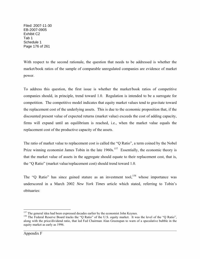
Filed: 2007-11-30 EB-2007-0905 Exhibit C2 Tab 1 Schedule 1 Page 176 of 261
______________________________________________________________________________ Appendix F
With respect to the second rationale, the question that needs to be addressed is whether the
market/book ratios of the sample of comparable unregulated companies are evidence of market
power.
To address this question, the first issue is whether the market/book ratios of competitive
companies should, in principle, trend toward 1.0. Regulation is intended to be a surrogate for
competition. The competitive model indicates that equity market values tend to gravitate toward
the replacement cost of the underlying assets. This is due to the economic proposition that, if the
discounted present value of expected returns (market value) exceeds the cost of adding capacity,
firms will expand until an equilibrium is reached, i.e., when the market value equals the
replacement cost of the productive capacity of the assets.
The ratio of market value to replacement cost is called the “Q Ratio”, a term coined by the Nobel
Prize winning economist James Tobin in the late 1960s.157 Essentially, the economic theory is
that the market value of assets in the aggregate should equate to their replacement cost, that is,
the “Q Ratio” (market value/replacement cost) should trend toward 1.0.
The “Q Ratio” has since gained stature as an investment tool,158 whose importance was
underscored in a March 2002 New York Times article which stated, referring to Tobin’s
obituaries:
157 The general idea had been expressed decades earlier by the economist John Keynes. 158 The Federal Reserve Board tracks the “Q Ratio” of the U.S. equity market. It was the level of the “Q Ratio”, along with the price/dividend ratio, that led Fed Chairman Alan Greenspan to warn of a speculative bubble in the equity market as early as 1996.
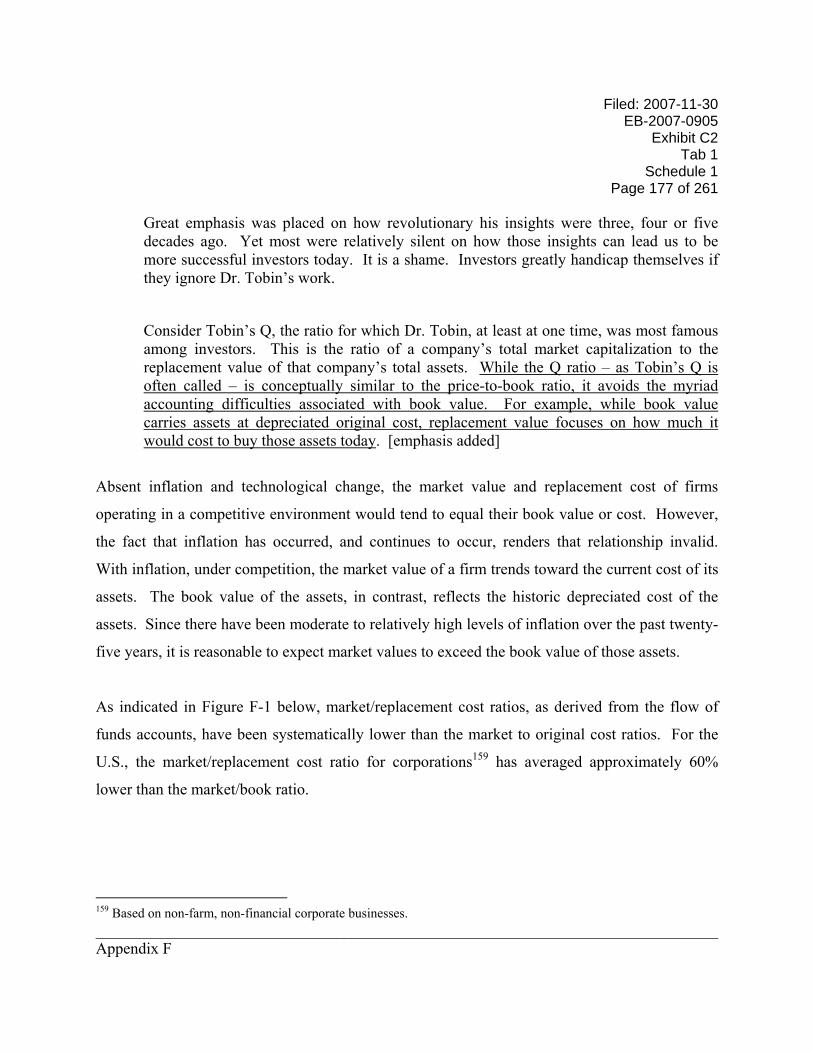
Filed: 2007-11-30 EB-2007-0905
Exhibit C2 Tab 1
Schedule 1 Page 177 of 261
______________________________________________________________________________ Appendix F
Great emphasis was placed on how revolutionary his insights were three, four or five decades ago. Yet most were relatively silent on how those insights can lead us to be more successful investors today. It is a shame. Investors greatly handicap themselves if they ignore Dr. Tobin’s work.
Consider Tobin’s Q, the ratio for which Dr. Tobin, at least at one time, was most famous among investors. This is the ratio of a company’s total market capitalization to the replacement value of that company’s total assets. While the Q ratio – as Tobin’s Q is often called – is conceptually similar to the price-to-book ratio, it avoids the myriad accounting difficulties associated with book value. For example, while book value carries assets at depreciated original cost, replacement value focuses on how much it would cost to buy those assets today. [emphasis added]
Absent inflation and technological change, the market value and replacement cost of firms
operating in a competitive environment would tend to equal their book value or cost. However,
the fact that inflation has occurred, and continues to occur, renders that relationship invalid.
With inflation, under competition, the market value of a firm trends toward the current cost of its
assets. The book value of the assets, in contrast, reflects the historic depreciated cost of the
assets. Since there have been moderate to relatively high levels of inflation over the past twenty-
five years, it is reasonable to expect market values to exceed the book value of those assets.
As indicated in Figure F-1 below, market/replacement cost ratios, as derived from the flow of
funds accounts, have been systematically lower than the market to original cost ratios. For the
U.S., the market/replacement cost ratio for corporations159 has averaged approximately 60%
lower than the market/book ratio.
159 Based on non-farm, non-financial corporate businesses.
Filed: 2007-11-30 EB-2007-0905 Exhibit C2 Tab 1 Schedule 1 Page 178 of 261
______________________________________________________________________________ Appendix F
Figure F-1
Q Ratio1952(Q1) to 2007(Q1)
0.00
0.50
1.00
1.50
2.00
2.50
3.00
1954
1956
1959
1962
1965
1967
1970
1973
1976
1978
1981
1984
1987
1989
1992
1995
1998
2000
2003
2006
Market/Replacement Market/Book
Source: US Federal Reserve Flow of Funds (B102).
To test the potential for market power in the achieved returns of the two samples of low risk
unregulated firms used in the comparable earnings test, their market/book ratios were compared
to those of the respective Canadian and U.S. market composites. The figure below tracks the
market/book values for the S&P/TSX Composite and the S&P 500 from 1980-2006.
Filed: 2007-11-30 EB-2007-0905
Exhibit C2 Tab 1
Schedule 1 Page 179 of 261
______________________________________________________________________________ Appendix F
Figure F-2
Market/Book Ratios
0.001.002.003.004.005.006.00
Dec
-79
Dec
-81
Dec
-83
Dec
-85
Dec
-87
Dec
-89
Dec
-91
Dec
-93
Dec
-95
Dec
-97
Dec
-99
Dec
-01
Dec
-03
Dec
-05
S&P 500 S&P/TSX
Source: RBC Capital Markets Quantitative Research
The data from which the table was created indicate that the market/book ratio for the overall
Canadian equity market has averaged approximately 1.7 times from 1980-2006, and
approximately 2.1 times from 1994-2006, the period over which the comparable earnings test
was conducted. Based on twenty-five years of data, the market/book ratio for the Canadian
equity market has varied around an average of close to 1.7 times, not 1.0 times. Over the period
1994-2006 the market/book ratio for the sample of comparable Canadian unregulated companies
averaged 2.1 times, equal to the average for the S&P/TSX Composite. For the S&P 500, the
market/book ratios were approximately 2.5 and 3.4 times, respectively, over the same two
periods. For the sample of low risk U.S. unregulated firms, the average market/book ratio was
2.7 times from 1994-2006. The similar to lower average market/book ratios of the low risk

Filed: 2007-11-30 EB-2007-0905 Exhibit C2 Tab 1 Schedule 1 Page 180 of 261
______________________________________________________________________________ Appendix F
samples relative to the overall equity market composites permit the inference that the sample
average returns are not characterized by market power.
In summary, the comparable earnings results do not warrant an adjustment for market/book
ratios.

Filed: 2007-11-30 EB-2007-0905
Exhibit C2 Tab 1
Schedule 1 Page 181 of 261
______________________________________________________________________________ Appendix G
APPENDIX G
FINANCING FLEXIBILITY ADJUSTMENT
An adjustment to the equity risk premium and discounted cash flow test results for financing
flexibility is required because the measurement of the return requirement based on market data
results in a "bare-bones" cost. It is “bare-bones” in the sense that, theoretically, if this return is
applied to (and earned on) the book equity of the rate base (assuming the expected return
corresponds to the approved return), the market value of the utility would be kept close to book
value.
The financing flexibility allowance is an integral part of the cost of capital as well as a required
element of the concept of a fair return. The allowance is intended to cover three distinct aspects:
(1) flotation costs, comprising financing and market pressure costs arising at the time of the sale
of new equity; (2) a margin, or cushion, for unanticipated capital market conditions; and (3) a
recognition of the "fairness" principle. Fairness dictates that regulation should not seek to keep
the market value of a utility stock close to book value when industrials of comparable investment
risk have been able to consistently maintain the real value of their assets considerably above
book value.
The financing flexibility allowance recognizes that return regulation remains, fundamentally, a
surrogate for competition. Competitive industrials of reasonably similar risk to utilities have
consistently been able to maintain the real value of their assets significantly in excess of book
value, consistent with the proposition that, under competition, market value will tend to equal the
replacement cost, not the book value, of assets.

Filed: 2007-11-30 EB-2007-0905 Exhibit C2 Tab 1 Schedule 1 Page 182 of 261
______________________________________________________________________________ Appendix G
Utility return regulation should not seek to target the market/book ratios achieved by such
industrials, but, at the same time, it should not preclude utilities from achieving a level of
financial integrity that gives some recognition to the longer run tendency for the market value of
industrials to equate to the replacement cost of their productive capacity. This is warranted not
only on grounds of fairness, but also on economic grounds, to avoid misallocation of capital
resources. To ignore these principles in determining an appropriate financing flexibility
allowance is to ignore the basic premise of regulation. The adjustment for financing flexibility
recognizes that the market return derived from the equity risk premium test needs to be translated
into a return that is fair and reasonable when applied to book value.
This premise was recognized by the Independent Assessment Team (IAT), retained by the
Alberta Department of Resource Development to determine the cost parameters for the Power
Purchase Arrangement (PPAs) for existing regulated generating plants, concluded in its 1999
report, regarding flotation costs,
This is sometimes associated with flotation costs but is more properly regarded as providing a financial cushion which is particularly applicable given the use of historic cost book values in traditional rate of return regulation in Canada. No such adjustment has ever been made in UK utility regulation cases which tend to use market values or current cost values.160
The Report of the IAT was accepted by the Alberta Energy and Utilities Board in Decision
U99113 (December 1999).
Further, the financing flexibility allowance should also recognize that both the equity risk
premium and DCF cost of equity estimates are derived from market values of equity capital. The
160Independent Assessment Team Power Purchase Arrangement Report, July 1999, page XLV, footnote 99.
Filed: 2007-11-30 EB-2007-0905
Exhibit C2 Tab 1
Schedule 1 Page 183 of 261
______________________________________________________________________________ Appendix G
cost of capital reflects the market value of the firms’ capital, both debt and equity. The market
value capital structures may be quite different from the book value capital structures. When the
market value common equity ratio is higher (lower) than the book value common equity ratio,
the market is attributing less (more) financial risk to the firm than is “on the books” as measured
by the book value capital structure. Higher financial risk leads to a higher cost of common
equity, all other things equal.
To put this concept in common sense terms, assume that I purchased my home 10 years ago for
$100,000. My home is currently worth $250,000. If I were applying for a loan, the bank would
consider my net worth (equity) to be $150,000, not the “book value” of my home, which reflects
the original purchase price less the mortgage loan amount. It is the market value of my home
that determines my financial risk to the bank, not the original purchase price. The same principle
applies when the cost of common equity is estimated. The book value of the common equity
shares is not the relevant measure of financial risk to equity investors; it is their market value,
that is, the value at which the shares could be sold.
Regulatory convention applies the allowed equity return to a book value capital structure. When
the market value equity ratios of the proxy utilities are well in excess of their book value
common equity ratios, application of an unadjusted market-derived cost of equity to the book
value capital structure fails to recognize the higher financial risk and the higher cost of equity
implied by the book value capital structures.
Two approaches can be used to quantify the range of the impact of a change in financial risk on
the cost of equity. The first approach is based on the theory that the overall cost of capital does
not change materially over a relatively broad range of capital structures. The second approach is

Filed: 2007-11-30 EB-2007-0905 Exhibit C2 Tab 1 Schedule 1 Page 184 of 261
______________________________________________________________________________ Appendix G
based on the theoretical model which assumes that the overall cost of capital declines as the debt
ratio rises due to the income tax shield on interest expense.161
Schedules 20 and 22 provide the formulas and inputs for estimating the change in the cost of
equity under each of the two approaches. The schedules show that a recognition of the
difference in financial risk between the market value and book value capital structures of the
publicly-traded Canadian utilities and the low risk U.S. utilities results in an increase in the cost
of equity in the range of 0.85 to 2.05 percentage points. A minimal recognition of the higher
financial risk in the book value capital structures supports a financing flexibility adjustment of no
less than 50 basis points.
At a minimum, the financing flexibility allowance should be adequate to allow a utility to
maintain its market value, notionally, at a slight premium to book value, i.e., in the range of 1.05-
1.10. At this level, a utility will be able to recover actual financing costs, as well as be in a
position to raise new equity (under most market conditions) without impairing its financial
integrity. A financing flexibility allowance adequate to maintain a market/book in the range of
1.05-1.10 is approximately 50 basis points.162
161 The second approach does not account for any of the factors that offset the corporate income tax advantage of debt, including the costs of bankruptcy/loss of financing flexibility, the impact of personal income taxes on the attractiveness of issuing debt, or the flow-through of the benefits of interest expense deductibility to ratepayers. Thus, the results of applying the second approach will over-estimate the impact of leverage on the overall cost of capital and understate the impact of increasing financial leverage on the cost of equity. 162 The financing flexibility allowance is estimated using the following formula developed from the discounted cash flow formula: Return on Book Equity = Market/Book Ratio x “bare-bones” Cost of Equity 1 + [retention rate (M/B – 1.0)] For a market/book ratio of 1.075 (mid-point of 1.05 and 1.10), assuming a dividend payout ratio of 65% and a cost of equity of 10.0%, the indicated ROE is:

Filed: 2007-11-30 EB-2007-0905
Exhibit C2 Tab 1
Schedule 1 Page 185 of 261
______________________________________________________________________________ Appendix G
The concept of a financing flexibility or flotation cost allowance has been accepted by most
Canadian regulators. As a government-owned utility, OPG does not raise capital in the public
equity markets; therefore it would not incur out-of-pocket equity financing and market pressure
costs. However, both the cushion, or safety margin, for unanticipated capital market conditions
and the fairness element are integral components of the cost of equity and a fair return on the
book value of equity. Both should be recognized in the allowed return on equity for a regulated
utility, irrespective of ownership.
OPG operates as a commercial entity. As such, the utility should be financed with a capital
structure that, similar to investor-owned utilities, reflects its business risks and, in principle,
would allow it to access the capital markets on reasonable terms and conditions on a stand-alone
basis. An investor-owned utility can access the public equity markets to finance its “normal”
capital program, as well as any extraordinary needs, and to maintain a balanced capital structure.
OPG’s access to equity is largely through retained earnings.
Consequently, OPG’s need for financing flexibility is no less than that of an investor-owned
utility. Thus, the financing allowance component of the fair return should be the same as for an
investor-owned utility. Explicit inclusion of a financing flexibility allowance in the ROE for a
government-owned utility has regulatory precedents. The government-owned utilities in both
British Columbia and Alberta have been allowed returns that are equivalent to those of the
ROE = 1.0)] - (1.075 [.35 1
10% x 1.075+
ROE = 10.5% The difference between the ROE and the “bare-bones” cost of equity of 50 basis points is the financing flexibility allowance.

Filed: 2007-11-30 EB-2007-0905 Exhibit C2 Tab 1 Schedule 1 Page 186 of 261
______________________________________________________________________________ Appendix G
investor-owned utilities, which, in turn, include an allowance for financing flexibility. In
Alberta, for example, in the recent Generic Cost of Capital decision (Decision 2004-052, July 2,
2004), the EUB allowed an adjustment of 50 basis points for flotation costs and financing
flexibility to all of the utilities to which the decision applied, both investor- and government-
owned.
The financing flexibility allowance for OPG should be, at a minimum, 50 basis points. As this
financing flexibility adjustment is minimal, it does not fully address the comparable earnings
standard.
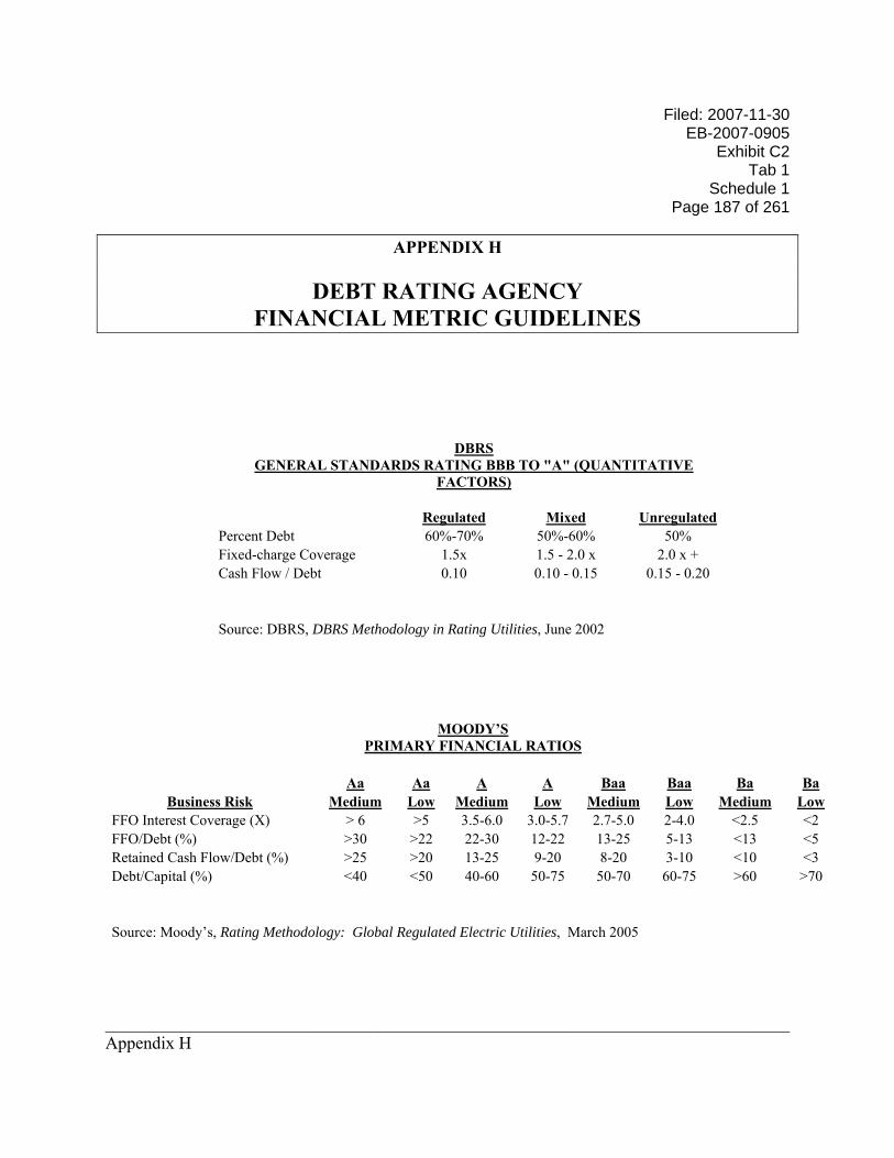
Filed: 2007-11-30 EB-2007-0905
Exhibit C2 Tab 1
Schedule 1 Page 187 of 261
______________________________________________________________________________ Appendix H
APPENDIX H
DEBT RATING AGENCY FINANCIAL METRIC GUIDELINES
DBRS GENERAL STANDARDS RATING BBB TO "A" (QUANTITATIVE
FACTORS)
Regulated Mixed Unregulated Percent Debt 60%-70% 50%-60% 50% Fixed-charge Coverage 1.5x 1.5 - 2.0 x 2.0 x + Cash Flow / Debt 0.10 0.10 - 0.15 0.15 - 0.20 Source: DBRS, DBRS Methodology in Rating Utilities, June 2002
MOODY’S PRIMARY FINANCIAL RATIOS
Aa Aa A A Baa Baa Ba Ba
Business Risk Medium Low Medium Low Medium Low Medium Low FFO Interest Coverage (X) > 6 >5 3.5-6.0 3.0-5.7 2.7-5.0 2-4.0 <2.5 <2 FFO/Debt (%) >30 >22 22-30 12-22 13-25 5-13 <13 <5 Retained Cash Flow/Debt (%) >25 >20 13-25 9-20 8-20 3-10 <10 <3 Debt/Capital (%) <40 <50 40-60 50-75 50-70 60-75 >60 >70 Source: Moody’s, Rating Methodology: Global Regulated Electric Utilities, March 2005
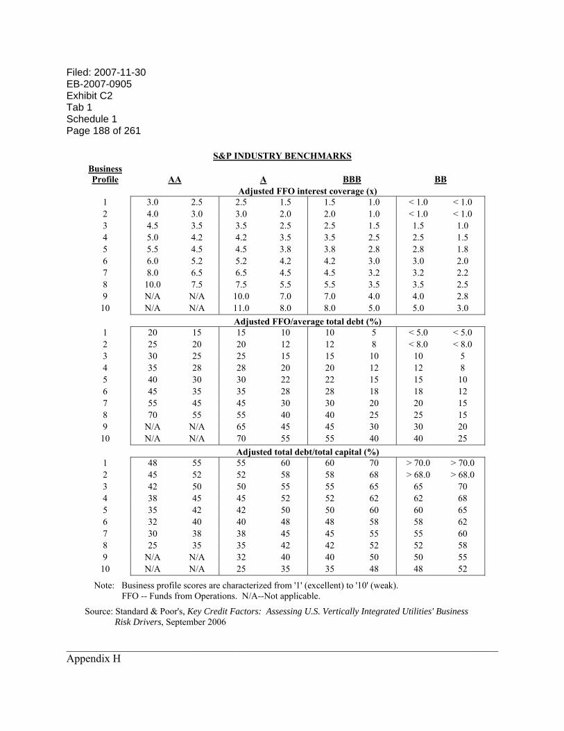
Filed: 2007-11-30 EB-2007-0905 Exhibit C2 Tab 1 Schedule 1 Page 188 of 261
______________________________________________________________________________ Appendix H
S&P INDUSTRY BENCHMARKS Business Profile AA A BBB BB
Adjusted FFO interest coverage (x) 1 3.0 2.5 2.5 1.5 1.5 1.0 < 1.0 < 1.0 2 4.0 3.0 3.0 2.0 2.0 1.0 < 1.0 < 1.0 3 4.5 3.5 3.5 2.5 2.5 1.5 1.5 1.0 4 5.0 4.2 4.2 3.5 3.5 2.5 2.5 1.5 5 5.5 4.5 4.5 3.8 3.8 2.8 2.8 1.8 6 6.0 5.2 5.2 4.2 4.2 3.0 3.0 2.0 7 8.0 6.5 6.5 4.5 4.5 3.2 3.2 2.2 8 10.0 7.5 7.5 5.5 5.5 3.5 3.5 2.5 9 N/A N/A 10.0 7.0 7.0 4.0 4.0 2.8
10 N/A N/A 11.0 8.0 8.0 5.0 5.0 3.0 Adjusted FFO/average total debt (%) 1 20 15 15 10 10 5 < 5.0 < 5.0 2 25 20 20 12 12 8 < 8.0 < 8.0 3 30 25 25 15 15 10 10 5 4 35 28 28 20 20 12 12 8 5 40 30 30 22 22 15 15 10 6 45 35 35 28 28 18 18 12 7 55 45 45 30 30 20 20 15 8 70 55 55 40 40 25 25 15 9 N/A N/A 65 45 45 30 30 20
10 N/A N/A 70 55 55 40 40 25 Adjusted total debt/total capital (%) 1 48 55 55 60 60 70 > 70.0 > 70.0 2 45 52 52 58 58 68 > 68.0 > 68.0 3 42 50 50 55 55 65 65 70 4 38 45 45 52 52 62 62 68 5 35 42 42 50 50 60 60 65 6 32 40 40 48 48 58 58 62 7 30 38 38 45 45 55 55 60 8 25 35 35 42 42 52 52 58 9 N/A N/A 32 40 40 50 50 55
10 N/A N/A 25 35 35 48 48 52
Note: Business profile scores are characterized from '1' (excellent) to '10' (weak). FFO -- Funds from Operations. N/A--Not applicable. Source: Standard & Poor's, Key Credit Factors: Assessing U.S. Vertically Integrated Utilities' Business Risk Drivers, September 2006
Filed: 2007-11-30 EB-2007-0905
Exhibit C2 Tab 1
Schedule 1 Page 189 of 261
______________________________________________________________________________ Appendix I
APPENDIX I
TRANSLATION OF RETURN REQUIREMENT TO COMMON EQUITY RATIO
BACKGROUND
The benchmark utility return was developed from market data for all publicly traded Canadian
utilities and a sample of low risk U.S. utilities determined to be of equivalent risk to a benchmark
Canadian utility. OPG faces higher business risk than the typical Canadian utility and the sample
of low risk U.S. utilities used in the estimation of the benchmark return on equity. The objective
of this appendix is to quantify the deemed common equity ratio for OPG’s regulated operations
that is required to equate OPG’s total business and financial risk to that of a benchmark utility.
At the identified common equity ratio, the benchmark utility return on equity will be applicable
to OPG.
METHODOLOGY
To quantify the equity ratio required for the benchmark utility return on equity to be applicable
to OPG, the following steps were taken:
Filed: 2007-11-30 EB-2007-0905 Exhibit C2 Tab 1 Schedule 1 Page 190 of 261
______________________________________________________________________________ Appendix I
Select a sample of vertically integrated U.S. utilities that have a significant proportion of their
assets devoted to generation (“high Gx”), i.e., that are closer in business risk to OPG’s regulated
operations than the low risk U.S. utility sample. 163
1. Estimate the betas and CAPM costs of equity for the “high Gx” utility sample.
2. Disaggregate the betas for the “high Gx” sample companies to derive an estimate of the
betas for the generation-only portion of their businesses.
a. Select a sample of “wires-only” utilities and use to estimate the “wires-only” beta.
b. Determine the proportion of assets for each company in the “high Gx” sample
devoted to generation, wires and “other operations”.
c. Using the estimated beta for wires and assuming a market average beta of 1.0 for
“other operations”, derive the generation-only betas.
3. Combine the generation-only betas with my estimates of the market risk premium and
risk-free rate to arrive at an estimate of the generation-only CAPM cost of equity. Since
the capital structures of both samples (wires, and high Gx) used to derive the generation-
only betas each contain close to 45% equity, the generation-only return requirement
would apply to OPG’s regulated operations as estimated if OPG’s deemed common
equity ratio were set at 45%.
163 The capital markets in the U.S. and Canada are significantly integrated; there are no publicly traded companies in Canada with nuclear assets. Based on Standard & Poor’s comments that due to deregulation in European power markets (S&P, “Credit Aspects of North American and European Nuclear Power”, January 2006), nuclear operators were offered no regulatory protection, we concluded that any investor-owned companies with nuclear facilities were not directly comparable to OPG.
Filed: 2007-11-30 EB-2007-0905
Exhibit C2 Tab 1
Schedule 1 Page 191 of 261
______________________________________________________________________________ Appendix I
4. Compare the capital structures for the benchmark low risk U.S. utility sample to the
capital structures for the “wires” and “high Gx” samples to determine the extent to which
differences in betas among samples are due to differences in financial risk versus
business risk.164
5. Compare the betas for the benchmark low risk U.S. utility sample to those of the “high
Gx” sample as well as to the generation-only betas and DCF costs derived from the “high
Gx sample.
6. Use the difference between the benchmark low risk U.S. sample beta and the “high Gx”
and generation-only betas in conjunction with the market risk premium to estimate the
incremental (to the benchmark return) equity return requirement for a utility of similar
business risk to OPG at a 45% common equity ratio.
7. Based on capital structure theory (discussed at page I-8 and I-9), translate the incremental
required return at a 45% common equity ratio into the common equity ratio which would
eliminate the need for an incremental return, i.e., would equate the equity return
requirement of OPG’s regulated operations to the benchmark return.
164 The betas used to estimate the generation-only beta were investment risk betas, that is, they comprise both business and financial risk. To the extent that the samples have different capital structures (and thus different levels of financial risk), business risk betas rather than the traditional investment risk betas would need to be calculated and used. By isolating the financial risk from the business risk, the incremental cost of capital arising from exposure to the business risks of generation can then be estimated.
Filed: 2007-11-30 EB-2007-0905 Exhibit C2 Tab 1 Schedule 1 Page 192 of 261
______________________________________________________________________________ Appendix I
1. Selection of Vertically Integrated Utility Sample
A sample of U.S. vertically integrated utilities with a high proportion of their assets
devoted to generation was selected, comprised of all utilities satisfying the following
criteria:
a. Classified by Value Line as an electric utility; b. Standard & Poor’s debt rating of BBB- or higher; c. I/B/E/S long-term earnings growth forecasts available; d. Paid a dividend in 2006; and, e. Generation assets comprising one-third or more of total assets.
The 21 utilities that met these criteria are listed on Schedule 28. The sample has a median S&P
debt rating of BBB. The average proportion of generation assets to total assets for the sample is
approximately 49%, with 16 of the sample companies having nuclear generation assets. Based
on 2006 production in MWs, nuclear generation accounted for approximately 10%. The “wires”
operations of the high generation sample comprised approximately 44% of total assets; “other
operations” accounted for approximately 7% of the total assets.
Filed: 2007-11-30 EB-2007-0905
Exhibit C2 Tab 1
Schedule 1 Page 193 of 261
______________________________________________________________________________ Appendix I
2. Betas and CAPM Cost of Equity for the High Generation Sample
The beta for the “High Gx” utility sample was estimated to be approximately 0.84 based on both
the Value Line and Standard & Poor’s adjusted betas165 for the firms in the sample.166
The Value Line and S&P betas are as follows:
Table I-1
Value Line S&P Adjusted
Mean 0.93 0.77
Median 0.95 0.81
Asset-Weighted Average 0.93 0.68
Source: Schedule 28.
The market risk premium and risk free rate used to deriving the CAPM costs of equity were the
same 6.50% and 5.0% used in the development of the benchmark return on equity. At a 0.84
beta, the CAPM cost of equity for the high generation utility sample is approximately 10.5%,
compared to approximately 9.5% for the low risk utility U.S. sample used to establish the
benchmark return on equity (beta of 0.71). 165 “Raw” betas were calculated using 60 monthly observations using the S&P 500 as the market index. The betas were adjusted using the following formula: ⅔ (“raw” beta) + ⅓ (market beta of 1.0). Value Line, Bloomberg and Merrill Lynch, major sources of financial information for investors, all publish adjusted betas. Their formulas for adjusting the calculated raw betas are slightly different, but all give approximately two-thirds weight to the “raw” beta of the specific stock and one-third weight to the market beta of 1.0. 166 The 0.84 beta represents the average of the simple mean, median, and asset-weighted average betas of the sample.

Filed: 2007-11-30 EB-2007-0905 Exhibit C2 Tab 1 Schedule 1 Page 194 of 261
______________________________________________________________________________ Appendix I
3. Estimation of a Generation-Only Beta
Using the residual beta methodology, the generation-only beta was estimated from the beta of the
high generation sample. The “residual beta” methodology is described in Roger Morin, New
Regulatory Finance, Vienna, VA: Public Utilities Reports, Inc., 2006. It is based on the Capital
Asset Pricing Model, which holds that the beta of a portfolio is the market value weighted
average of the betas of the investments that make up the portfolio. The notion that the beta of a
firm is equal to the weighted average of its divisional betas is a foundation for the “pure play”
technique of estimating the betas for individual divisions of a multi-division firm. As stated in
Russell J. Fuller and Halbert S. Kerr, “Estimating the Divisional Cost of Capital: An Analysis of
the Pure-Play Technique,” Journal of Finance, December 1981, “it can be shown that the beta
for a multidivisional firm approximates the weighted average of its divisional betas”. The pure
play technique estimates the divisional betas using the betas of proxy firms. The proxy firms for
each division operate in a single line of business (pure play), the same line of business as the
individual divisions of the multi-division company.
The residual beta methodology is used to estimate the beta of a division for which there are no
pure play proxies. The methodology entails disaggregating the beta of a multi-divisional firm
into the betas of its divisions. Its application requires the beta of the firm as a whole and a “pure
play” beta for each of the divisions other than the one for which there are no pure play proxies.
In the disaggregation of the company beta into the divisional betas, the weights to be given to
each division should be equal to their relative contribution to the operating income of the
consolidated entity. For the purpose of this analysis, I have used assets as a proxy for the relative
Filed: 2007-11-30 EB-2007-0905
Exhibit C2 Tab 1
Schedule 1 Page 195 of 261
______________________________________________________________________________ Appendix I
contribution of each division (or business segment) to the company as a whole. The
disaggregation formula for estimating the generation-only beta is:
βHighGx = βGx x %AssetsGx + βPure Wires x %AssetsWires + βOther x %AssetsOther
The Wires beta was developed from a sample of Wires utilities. A Wires sample was selected,
comprised of all U.S. utilities satisfying the following criteria:
a. classified by Value Line as an electric or gas distribution utility;
b. with at least 80% of total assets devoted to electricity and gas distribution
operations;
c. has no more than 5% of its assets in generation;
d. whose Standard & Poor’s debt rating is BBB- or higher; and,
e. has I/B/E/S forecasts.167
The 8 firms in the sample are found in Schedule 29. Wires assets account for 96% (average) of
the total assets of the sample companies. The sample has a median S&P debt rating of A.
The beta for the “Wires” sample was estimated to be 0.72 based on both the Value Line and
Standard & Poor’s adjusted betas the firms in the sample.
167 The existence of I/B/E/S forecasts ensures that the utilities have an analyst following, which in turn, ensures that the companies shares are traded frequently enough so that the betas are meaningful.
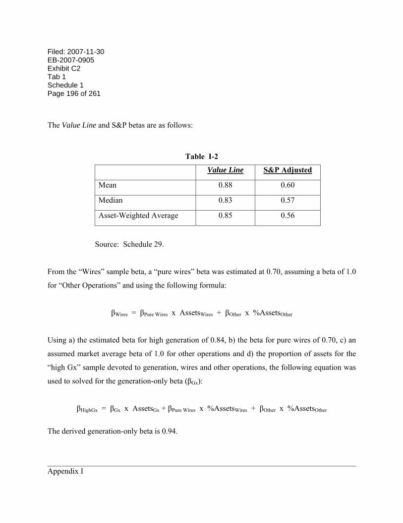
Filed: 2007-11-30 EB-2007-0905 Exhibit C2 Tab 1 Schedule 1 Page 196 of 261
______________________________________________________________________________ Appendix I
The Value Line and S&P betas are as follows:
Table I-2
Value Line S&P Adjusted
Mean 0.88 0.60
Median 0.83 0.57
Asset-Weighted Average 0.85 0.56
Source: Schedule 29.
From the “Wires” sample beta, a “pure wires” beta was estimated at 0.70, assuming a beta of 1.0
for “Other Operations” and using the following formula:
βWires = βPure Wires x AssetsWires + βOther x %AssetsOther
Using a) the estimated beta for high generation of 0.84, b) the beta for pure wires of 0.70, c) an
assumed market average beta of 1.0 for other operations and d) the proportion of assets for the
“high Gx” sample devoted to generation, wires and other operations, the following equation was
used to solved for the generation-only beta (βGx):
βHighGx = βGx x AssetsGx + βPure Wires x %AssetsWires + βOther x %AssetsOther
The derived generation-only beta is 0.94.

Filed: 2007-11-30 EB-2007-0905
Exhibit C2 Tab 1
Schedule 1 Page 197 of 261
______________________________________________________________________________ Appendix I
4. Derivation of Generation-Only CAPM Cost of Equity
The generation-only beta of 0.94 was combined with the estimates of the market risk premium
and risk-free rate to arrive at an estimate of the generation-only CAPM cost of equity of
approximately 11.1%.
5. Comparison of Sample Capital Structures
The capital structures for the benchmark low risk U.S. utility sample, the “wires”, and the “high
Gx” samples were compared to determine the extent to which differences in betas among
samples are due to differences in financial risk versus business risk. Since the common equity
ratio of each of the three samples was approximately 45%, any difference in betas among the
samples could be attributed to business risk. The table below compares the 2006 equity ratios of
the benchmark low risk utility sample, the “wires” sample and the “high Gx” sample.
Table I-3
Benchmark Wires High Gx
Mean 44.9% 44.9% 44.8%
Median 44.6% 47.0% 45.8%
Weighted Average 43.5% 44.2% 43.0%
Source: Schedules 13, 28 and 29
Filed: 2007-11-30 EB-2007-0905 Exhibit C2 Tab 1 Schedule 1 Page 198 of 261
______________________________________________________________________________ Appendix I
6. Comparison of Betas
The betas of the benchmark low risk utility U.S. utility sample, the “high Gx” sample and the
derived generation-only beta are respectively 0.71, 0.84 and 0.94.
7. Calculation of the Incremental Cost of Equity at a 45% Common Equity Ratio
The differences between the beta for the benchmark low risk U.S. utility sample (0.71) and those
of the “high Gx” sample (0.84) and the derived generation-only beta (0.94) were determined.
These differences, in conjunction with estimated market risk premium, were used to estimate the
incremental cost of equity for a utility of similar risk to OPG at a 45% common equity ratio. The
incremental return requirement was calculated as follows:
Incremental Return Requirement at 45% Equity = Difference in Beta x Market Risk Premium
Based on the high generation sample, the incremental equity return requirement is equal to
approximately 85 basis points; based on the derived generation-only betas, the incremental
equity return requirement is approximately 150 basis points, estimated as follows:
Filed: 2007-11-30 EB-2007-0905
Exhibit C2 Tab 1
Schedule 1 Page 199 of 261
______________________________________________________________________________ Appendix I
Incremental Equity Return = (βHighGx - βBenchmark Sample) x MRP
= (0.84-0.71) X 6.5%
= 0.85%
Incremental Equity Return = (βGx - βBenchmark Sample) x MRP
= (0.94-0.71) X 6.5%
= 1.50%
8. Application of Capital Structure Theory
Based on both the high generation sample beta and the derived generation-only betas compared
to the benchmark low risk utility sample beta, the incremental required equity return for OPG’s
regulated operations at a 45% common equity ratio – equal to the common equity ratios of the
samples – is in the range of 0.85% to 1.50%. Since OPG’s regulated operations are 100%
generation, the focus should be on the upper end of the range, i.e. in the range of approximately
1.25% to 1.50%. Thus, compared to the benchmark return on equity of 10.5%, which is based
on the application of multiple tests, the return on equity for OPG at a 45% common equity ratio
would be approximately 11.75% to 12.0%.
Using capital structure theory, the incremental required return at a 45% common equity ratio can
be translated into the common equity ratio which would eliminate the need for an incremental
return, i.e., would equate the return requirement of OPG’s regulated operations to the benchmark
return.

Filed: 2007-11-30 EB-2007-0905 Exhibit C2 Tab 1 Schedule 1 Page 200 of 261
______________________________________________________________________________ Appendix I
The estimation of the change in equity ratio for a given change in equity return is based on two
different theories of the relationship between capital structure and return on equity. Theory 1
posits that income taxes and the deductibility of interest for corporate income tax purposes have
no impact on the cost of capital. Under this theory, the overall cost of capital stays constant
when the capital structure changes, although the costs of the debt and equity components change
(i.e., the cost of equity rises when the equity ratio declines). Theory 2 posits that income taxes
and the corporate deductibility of interest expense cause the overall cost of capital to continually
decline as the equity ratio declines and the debt ratio increases. The underlying formulas for the
two theories are contained in Schedule 31.168
The actual impact on the cost of capital most likely lies in between the results of the two
theories; income taxes and the deductibility of interest do tend to decrease the cost of capital (as
the income trust market has demonstrated), but as the debt ratio rises, there are increasing costs
in terms of loss of financing flexibility and potential bankruptcy. Moreover, in the case of
regulated companies, the benefit of the tax deductibility of interest is to the benefit of ratepayers,
while in the unregulated sector, the benefit goes to the shareholder. Since both theories have
merit, both were applied to estimate the impact of a change in return on equity on capital
structure.
The table below indicates that, based on both theories, the range of common equity ratios
required to equate an 11.75-12.0% return on equity for OPG’s regulated operations at a 45%
168 The inputs for the derivation of the common equity ratio required to equate the return requirement of OPG’s regulated operations to the benchmark return include a cost of new long-term debt of 6.0% and a corporate income tax rate of 34%.
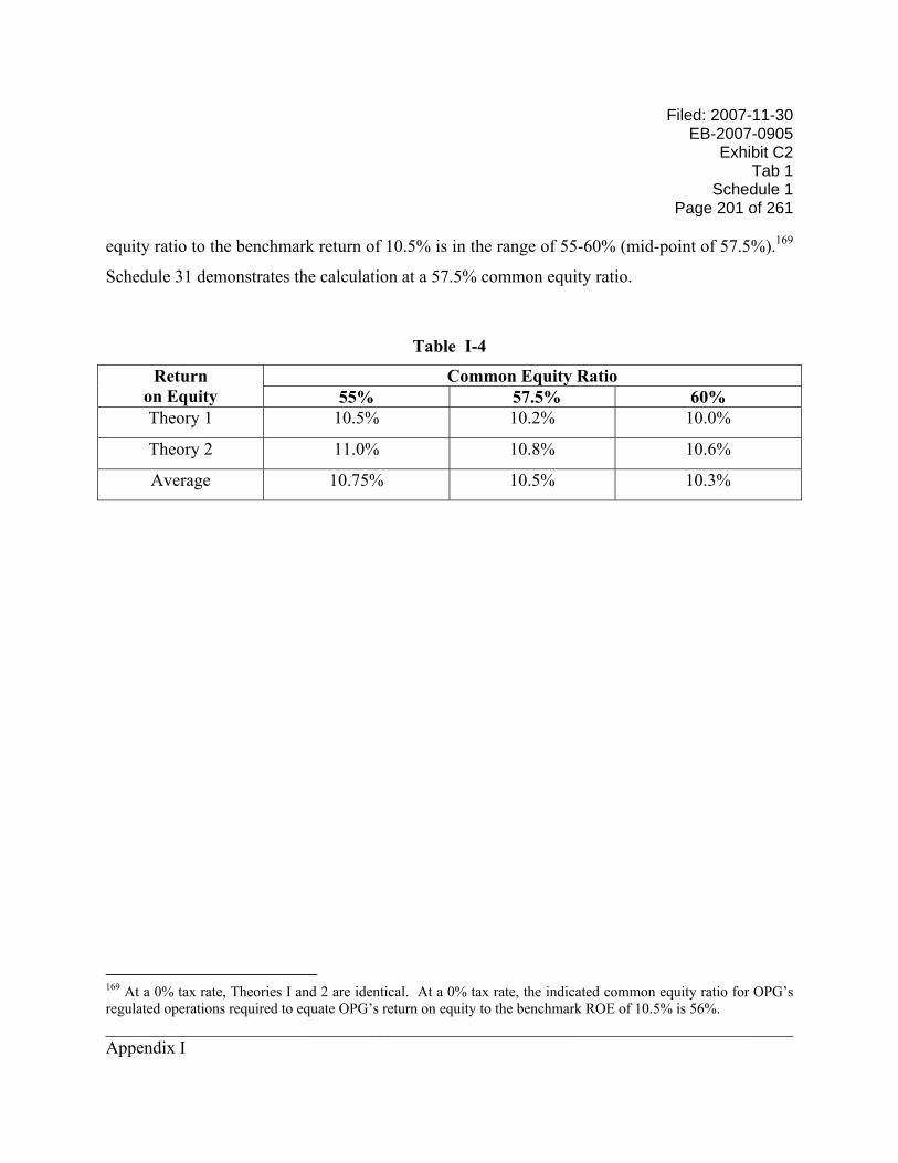
Filed: 2007-11-30 EB-2007-0905
Exhibit C2 Tab 1
Schedule 1 Page 201 of 261
______________________________________________________________________________ Appendix I
equity ratio to the benchmark return of 10.5% is in the range of 55-60% (mid-point of 57.5%).169
Schedule 31 demonstrates the calculation at a 57.5% common equity ratio.
Table I-4
Common Equity Ratio Return on Equity 55% 57.5% 60% Theory 1 10.5% 10.2% 10.0%
Theory 2 11.0% 10.8% 10.6%
Average 10.75% 10.5% 10.3%
169 At a 0% tax rate, Theories I and 2 are identical. At a 0% tax rate, the indicated common equity ratio for OPG’s regulated operations required to equate OPG’s return on equity to the benchmark ROE of 10.5% is 56%.

Filed: 2007-11-30 EB-2007-0905 Exhibit C2 Tab 1 Schedule 1 Page 202 of 261
______________________________________________________________________________ Appendix J
APPENDIX J
QUALIFICATIONS OF KATHLEEN C. McSHANE
Kathleen McShane is President and senior consultant with Foster Associates, Inc., where she has
been employed since 1981. She holds an M.B.A. degree in Finance from the University of
Florida, and M.A. and B.A. degrees from the University of Rhode Island. She has been a CFA
charterholder since 1989.
Ms. McShane worked for the University of Florida and its Public Utility Research Center,
functioning as a research and teaching assistant, before joining Foster Associates. She taught
both undergraduate and graduate classes in financial management and assisted in the preparation
of a financial management textbook.
At Foster Associates, Ms. McShane has worked in the areas of financial analysis, energy
economics and cost allocation. Ms. McShane has presented testimony in more than 150
proceedings on rate of return and capital structure before federal, state, provincial and territorial
regulatory boards, on behalf of U.S. and Canadian telephone companies, gas pipelines and
distributors, and electric utilities. These testimonies include the assessment of the impact of
business risk factors (e.g., competition, rate design, contractual arrangements) on capital
structure and equity return requirements. She has also testified on various ratemaking issues,
including deferral accounts, rate stabilization mechanisms, excess earnings accounts, cash
working capital, and rate base issues. Ms. McShane has provided consulting services for
numerous U.S. and Canadian companies on financial and regulatory issues, including financing,
dividend policy, corporate structure, cost of capital, automatic adjustments for return on equity,

Filed: 2007-11-30 EB-2007-0905
Exhibit C2 Tab 1
Schedule 1 Page 203 of 261
______________________________________________________________________________ Appendix J
form of regulation (including performance-based regulation), unbundling, corporate separations,
stand-alone cost of debt, regulatory climate, income tax allowance for partnerships, change in
fiscal year end, treatment of inter-corporate financial transactions, and the impact of weather
normalization on risk.
Ms. McShane was principal author of a study on the applicability of alternative incentive
regulation proposals to Canadian gas pipelines. She was instrumental in the design and
preparation of a study of the profitability of 25 major U.S. gas pipelines, in which she developed
estimates of rate base, capital structure, profit margins, unit costs of providing services, and
various measures of return on investment. Other studies performed by Ms. McShane include a
comparison of municipal and privately owned gas utilities, an analysis of the appropriate
capitalization and financing for a new gas pipeline, risk/return analyses of proposed water and
gas distribution companies and an independent power project, pros and cons of performance-
based regulation, and a study on pricing of a competitive product for the U.S. Postal Service.
She has also conducted seminars on cost of capital for regulated utilities, with focus on the
Canadian regulatory arena.
Filed: 2007-11-30 EB-2007-0905 Exhibit C2 Tab 1 Schedule 1 Page 204 of 261
______________________________________________________________________________ Appendix J
Publications, Papers and Presentations ■ “Utility Cost of Capital Canada vs. U.S.”, presented at the CAMPUT Conference, May
2003. ■ “The Effects of Unbundling on a Utility’s Risk Profile and Rate of Return”, (co-authored
with Owen Edmondson, Vice President of ATCO Electric), presented at the Unbundling Rates Conference, New Orleans, Louisiana sponsored by Infocast, January 2000.
■ Atlanta Gas Light’s Unbundling Proposal: More Unbundling Required?” presented at the
24th Annual Rate Symposium, Kansas City, Missouri, sponsored by several commissions and universities, April 1998.
■ “Incentive Regulation: An Alternative to Assessing LDC Performance”, (co-authored
with Dr. William G. Foster), presented at the Natural Gas Conference, Chicago, Illinois sponsored by the Center for Regulatory Studies, May 1993.
■ “Alternative Regulatory Incentive Mechanisms”, (co-authored with Stephen F. Sherwin),
prepared for the National Energy Board, Incentive Regulation Workshop, October 1992.
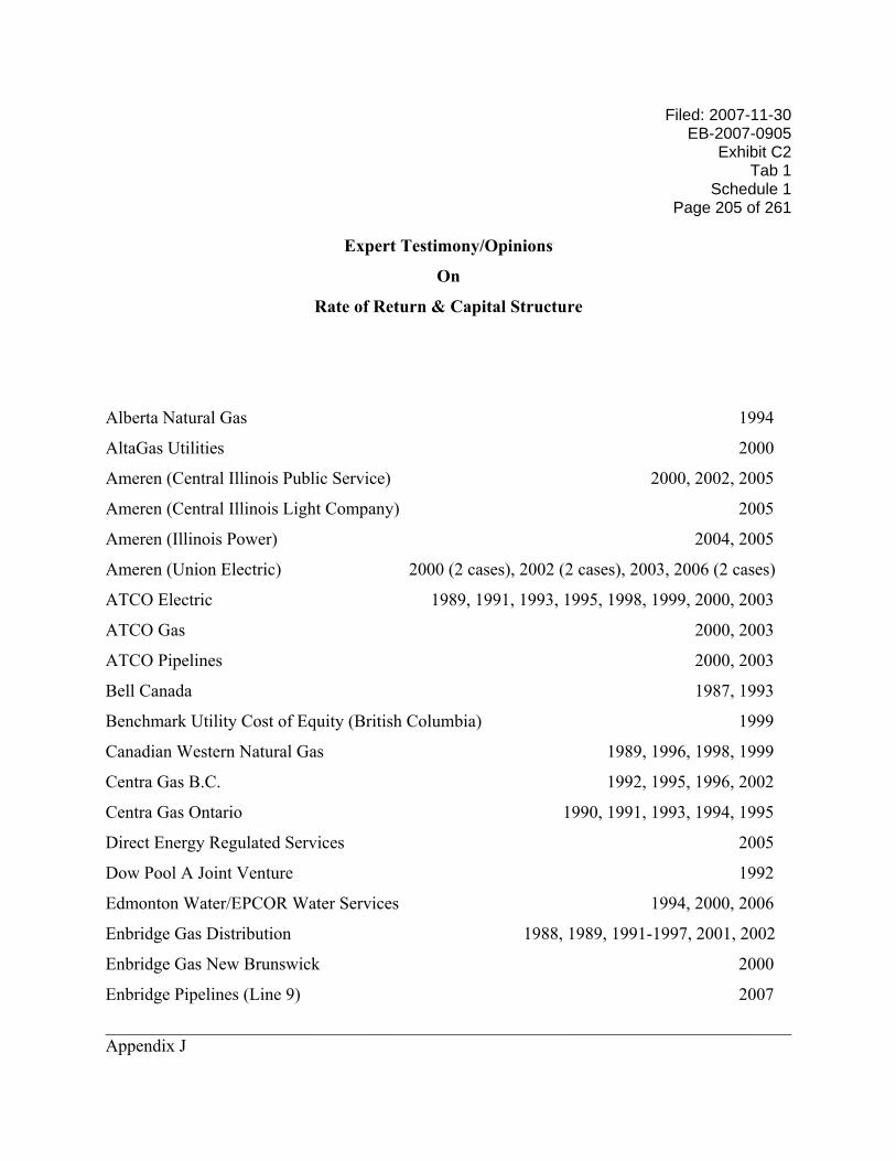
Filed: 2007-11-30 EB-2007-0905
Exhibit C2 Tab 1
Schedule 1 Page 205 of 261
______________________________________________________________________________ Appendix J
Expert Testimony/Opinions
On
Rate of Return & Capital Structure
Alberta Natural Gas 1994
AltaGas Utilities 2000
Ameren (Central Illinois Public Service) 2000, 2002, 2005
Ameren (Central Illinois Light Company) 2005
Ameren (Illinois Power) 2004, 2005
Ameren (Union Electric) 2000 (2 cases), 2002 (2 cases), 2003, 2006 (2 cases)
ATCO Electric 1989, 1991, 1993, 1995, 1998, 1999, 2000, 2003
ATCO Gas 2000, 2003
ATCO Pipelines 2000, 2003
Bell Canada 1987, 1993
Benchmark Utility Cost of Equity (British Columbia) 1999
Canadian Western Natural Gas 1989, 1996, 1998, 1999
Centra Gas B.C. 1992, 1995, 1996, 2002
Centra Gas Ontario 1990, 1991, 1993, 1994, 1995
Direct Energy Regulated Services 2005
Dow Pool A Joint Venture 1992
Edmonton Water/EPCOR Water Services 1994, 2000, 2006
Enbridge Gas Distribution 1988, 1989, 1991-1997, 2001, 2002
Enbridge Gas New Brunswick 2000
Enbridge Pipelines (Line 9) 2007
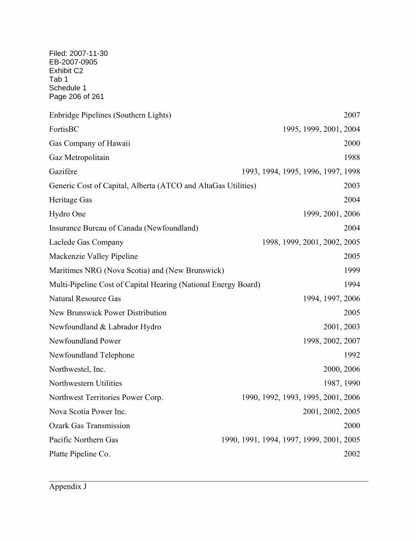
Filed: 2007-11-30 EB-2007-0905 Exhibit C2 Tab 1 Schedule 1 Page 206 of 261
______________________________________________________________________________ Appendix J
Enbridge Pipelines (Southern Lights) 2007
FortisBC 1995, 1999, 2001, 2004
Gas Company of Hawaii 2000
Gaz Metropolitain 1988
Gazifère 1993, 1994, 1995, 1996, 1997, 1998
Generic Cost of Capital, Alberta (ATCO and AltaGas Utilities) 2003
Heritage Gas 2004
Hydro One 1999, 2001, 2006
Insurance Bureau of Canada (Newfoundland) 2004
Laclede Gas Company 1998, 1999, 2001, 2002, 2005
Mackenzie Valley Pipeline 2005
Maritimes NRG (Nova Scotia) and (New Brunswick) 1999
Multi-Pipeline Cost of Capital Hearing (National Energy Board) 1994
Natural Resource Gas 1994, 1997, 2006
New Brunswick Power Distribution 2005
Newfoundland & Labrador Hydro 2001, 2003
Newfoundland Power 1998, 2002, 2007
Newfoundland Telephone 1992
Northwestel, Inc. 2000, 2006
Northwestern Utilities 1987, 1990
Northwest Territories Power Corp. 1990, 1992, 1993, 1995, 2001, 2006
Nova Scotia Power Inc. 2001, 2002, 2005
Ozark Gas Transmission 2000
Pacific Northern Gas 1990, 1991, 1994, 1997, 1999, 2001, 2005
Platte Pipeline Co. 2002
Filed: 2007-11-30 EB-2007-0905
Exhibit C2 Tab 1
Schedule 1 Page 207 of 261
______________________________________________________________________________ Appendix J
St. Lawrence Gas 1997, 2002
Southern Union Gas 1990, 1991, 1993
Stentor 1997
Tecumseh Gas Storage 1989, 1990
Telus Québec 2001
Terasen Gas 1992, 1994, 2005
TransCanada PipeLines 1988, 1989, 1991 (2 cases), 1992, 1993
TransGas and SaskEnergy LDC 1995
Trans Québec & Maritimes Pipeline 1987
Union Gas 1988, 1989, 1990, 1992, 1994, 1996, 1998, 2001
Westcoast Energy 1989, 1990, 1992 (2 cases), 1993, 2005
Yukon Electric Co. Ltd./Yukon Energy 1991, 1993
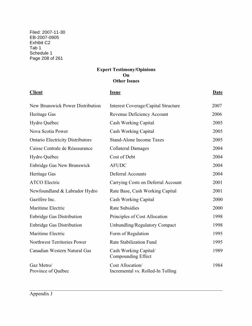
Filed: 2007-11-30 EB-2007-0905 Exhibit C2 Tab 1 Schedule 1 Page 208 of 261
______________________________________________________________________________ Appendix J
Expert Testimony/Opinions On
Other Issues
Client Issue Date
New Brunswick Power Distribution Interest Coverage/Capital Structure 2007
Heritage Gas Revenue Deficiency Account 2006
Hydro Québec Cash Working Capital 2005
Nova Scotia Power Cash Working Capital 2005
Ontario Electricity Distributors Stand-Alone Income Taxes 2005
Caisse Centrale de Réassurance Collateral Damages 2004
Hydro Québec Cost of Debt 2004
Enbridge Gas New Brunswick AFUDC 2004
Heritage Gas Deferral Accounts 2004
ATCO Electric Carrying Costs on Deferral Account 2001
Newfoundland & Labrador Hydro Rate Base, Cash Working Capital 2001
Gazifère Inc. Cash Working Capital 2000
Maritime Electric Rate Subsidies 2000
Enbridge Gas Distribution Principles of Cost Allocation 1998
Enbridge Gas Distribution Unbundling/Regulatory Compact 1998
Maritime Electric Form of Regulation 1995
Northwest Territories Power Rate Stabilization Fund 1995
Canadian Western Natural Gas Cash Working Capital/ Compounding Effect
1989
Gaz Metro/ Province of Québec
Cost Allocation/ Incremental vs. Rolled-In Tolling
1984
Filed: 2007-11-30 EB-2007-0905
Exhibit C2 Tab 1
Schedule 1 Page 209 of 261
STATISTICAL EXHIBIT TO
Capital Structure and Fair Return on Equity
Prepared for
ONTARIO POWER GENERATION
Prepared by
KATHLEEN C. McSHANE
FOSTER ASSOCIATES, INC.
November 2007
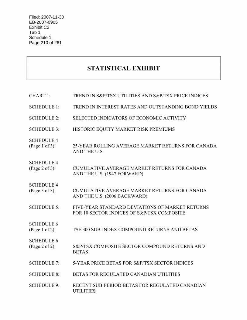
Filed: 2007-11-30 EB-2007-0905 Exhibit C2 Tab 1 Schedule 1 Page 210 of 261
STATISTICAL EXHIBIT
CHART 1: TREND IN S&P/TSX UTILITIES AND S&P/TSX PRICE INDICES SCHEDULE 1: TREND IN INTEREST RATES AND OUTSTANDING BOND YIELDS SCHEDULE 2: SELECTED INDICATORS OF ECONOMIC ACTIVITY SCHEDULE 3: HISTORIC EQUITY MARKET RISK PREMIUMS SCHEDULE 4 (Page 1 of 3): 25-YEAR ROLLING AVERAGE MARKET RETURNS FOR CANADA
AND THE U.S. SCHEDULE 4 (Page 2 of 3): CUMULATIVE AVERAGE MARKET RETURNS FOR CANADA
AND THE U.S. (1947 FORWARD) SCHEDULE 4 (Page 3 of 3): CUMULATIVE AVERAGE MARKET RETURNS FOR CANADA
AND THE U.S. (2006 BACKWARD) SCHEDULE 5: FIVE-YEAR STANDARD DEVIATIONS OF MARKET RETURNS
FOR 10 SECTOR INDICES OF S&P/TSX COMPOSITE SCHEDULE 6 (Page 1 of 2): TSE 300 SUB-INDEX COMPOUND RETURNS AND BETAS SCHEDULE 6 (Page 2 of 2): S&P/TSX COMPOSITE SECTOR COMPOUND RETURNS AND
BETAS SCHEDULE 7: 5-YEAR PRICE BETAS FOR S&P/TSX SECTOR INDICES SCHEDULE 8: BETAS FOR REGULATED CANADIAN UTILITIES SCHEDULE 9: RECENT SUB-PERIOD BETAS FOR REGULATED CANADIAN
UTILITIES
Filed: 2007-11-30 EB-2007-0905
Exhibit C2 Tab 1
Schedule 1 Page 211 of 261
SCHEDULE 10: HISTORIC UTILITY EQUITY RISK PREMIUMS SCHEDULE 11 (Page 1 of 3): 25-YEAR ROLLING AVERAGE RETURNS FOR CANADIAN & U.S.
UTILITIES AND GOVERNMENT BONDS SCHEDULE 11 (Page 2 of 3): CUMULATIVE AVERAGE RETURNS FOR CANADIAN & U.S.
UTILITIES AND GOVERNMENT BONDS (FORWARD) SCHEDULE 11 (Page 3 of 3): CUMULATIVE AVERAGE RETURNS FOR CANADIAN & U.S.
UTILITIES AND GOVERNMENT BONDS (BACKWARD) SCHEDULE 12: DCF-BASED EQUITY RISK PREMIUM STUDY FOR BENCHMARK
U.S. ELECTRIC AND GAS UTILITIES SCHEDULE 13: INDIVIDUAL COMPANY RISK DATA FOR BENCHMARK SAMPLE
OF U.S. ELECTRIC AND GAS UTILITIES SCHEDULE 14: DCF COST OF EQUITY FOR BENCHMARK SAMPLE OF U.S.
ELECTRIC AND GAS UTILITIES (BASED ON ANALYSTS’ EARNINGS GROWTH FORECASTS)
SCHEDULE 15: DCF COST OF EQUITY FOR BENCHMARK SAMPLE OF U.S.
ELECTRIC AND GAS UTILITIES (TWO STAGE MODEL) SCHEDULE 16: RISK MEASURES FOR 20 LOW RISK CANADIAN INDUSTRIALS SCHEDULE 17: RETURNS ON AVERAGE COMMON STOCK EQUITY FOR 20 LOW
RISK CANADIAN INDUSTRIALS SCHEDULE 18: RISK MEASURES FOR 157 LOW RISK U.S. INDUSTRIALS SCHEDULE 19: RETURNS ON AVERAGE COMMON STOCK EQUITY FOR 157
LOW RISK U.S. INDUSTRIALS SCHEDULE 20: ESTIMATE OF MARKET VALUE CAPITAL STRUCTURES FOR
CANADIAN UTILITIES SCHEDULE 21: ESTIMATE OF MARKET VALUE CAPITAL STRUCTURES FOR
BENCHMARK SAMPLE OF U.S. ELECTRIC AND GAS UTILITIES

Filed: 2007-11-30 EB-2007-0905 Exhibit C2 Tab 1 Schedule 1 Page 212 of 261
SCHEDULE 22: QUANTIFICATION OF IMPACT ON EQUITY RETURN REQUIREMENT FOR DIFFERENCE BETWEEN MARKET VALUE AND BOOK VALUE CAPITAL STRUCTURES: CANADIAN UTILITIES
SCHEDULE 23: QUANTIFICATION OF IMPACT ON EQUITY RETURN
REQUIREMENT FOR DIFFERENCE BETWEEN MARKET VALUE AND BOOK VALUE CAPITAL STRUCTURES: BENCHMARK LOW RISK U.S. GAS & ELECTRIC UTILITIES
SCHEDULE 24: CAPITAL STRUCTURE RATIOS OF CANADIAN UTILITIES SCHEDULE 25: FINANCIAL METRICS FOR CANADIAN UTILITIES SCHEDULE 26: DEBT AND COMMON STOCK QUALITY RATINGS OF CANADIAN
UTILITIES SCHEDULE 27: DEBT RATINGS AND FINANCIAL METRICS FOR U.S. ELECTRIC
UTILITIES SCHEDULE 28: INDIVIDUAL COMPANY RISK DATA FOR SAMPLE OF HIGH
GENERATION U.S. ELECTRIC UTILITIES SCHEDULE 29: INDIVIDUAL COMPANY RISK DATA FOR SAMPLE OF U.S.
WIRES UTILITIES SCHEDULE 30 (Page 1 of 3): EQUITY RETURN AWARDS AND CAPITAL STRUCTURES
ADOPTED BY REGULATORY BOARDS FOR CANADIAN UTILITIES
SCHEDULE 30 (Page 2 of 3): RATES OF RETURN ON COMMON EQUITY ADOPTED BY
REGULATORY BOARDS FOR INVESTOR-OWNED CANADIAN UTILITIES
SCHEDULE 30 (Page 2 of 3): COMPARISON BETWEEN ALLOWED EQUITY RISK PREMIUMS
FOR CANADIAN AND U.S. UTILITIES SCHEDULE 31: QUANTIFICATION OF IMPACT ON EQUITY RATIO
REQUIREMENT TO EQUATE EQUITY RETURN FOR OPG’S REGULATED OPERATIONS TO THE ROE REQUIRED FOR BENCHMARK LOW RISK U.S. GAS & ELECTRIC UTILITIES