international association of geodesy...

International Association of Geodesy Symposia

M ich ael G . Sideris, Series Editor

International Association of Geodesy Symposia

Symposium 101: Global and Regional Geodynamics Symposium 102: Global Positioning System: An Overview Symposium 103: Gravity, Gradiometry, and Gravimetry Symposium 104: Sea SurfaceTopography and the Geoid

Symposium 105: Earth Rotation and Coordinate Reference Frames Symposium 106: Determination of the Geoid: Present and Future

Symposium 107: Kinematic Systems in Geodesy, Surveying, and Remote Sensing Symposium 108: Application of Geodesy to Engineering

Symposium 109: Permanent Satellite Tracking Networks for Geodesy and Geodynamics Symposium 110: From Mars to Greenland: Charting Gravity with Space and Airborne Instruments

Symposium 111: Recent Geodetic and Gravimetric Research in Latin America Symposium 112: Geodesy and Physics of the Earth: Geodetic Contributions to Geodynamics

Symposium 113: Gravity and Geoid Symposium 114: Geodetic Theory Today

Symposium 115: GPS Trends in Precise Terrestrial, Airborne, and Spaceborne Applications Symposium 116: Global Gravity Field and Its Temporal Variations

Symposium 117: Gravity, Geoid and Marine Geodesy Symposium 118: Advances in Positioning and Reference Frames

Symposium 119: Geodesy on the Move Symposium 120: Towards an Integrated Global Geodetic Observation System (IGGOS)

Symposium 121: Geodesy Beyond 2000: The Challenges of the First Decade Symposium 122: IV Hotine-Marussi Symposium on Mathematical Geodesy

Symposium 123: Gravity, Geoid and Geodynamics 2000 Symposium 124: Vertical Reference Systems

Symposium 125: Vistas for Geodesy in the New Millennium Symposium 126: Satellite Altimetry for Geodesy, Geophysics and Oceanography

Symposium 127: V Hotine Marussi Symposium on Mathematical Geodesy Symposium 128: A Window on the Future of Geodesy Symposium 129: Gravity, Geoid and Space Missions

Symposium 130: Dynamic Planet - Monitoring and Understanding … Symposium 131: Geodetic Deformation Monitoring: From Geophysical to Engineering Roles Symposium 132: VI Hotine-Marussi Symposium on Theoretical and Computational Geodesy

M ich ael G . Sideris, Series Editor

Symposium 133: Observing our Changing EarthSymposium 134: Geodetic Reference Frames

Edited by

123

Geodetic Reference Frames

IAG SymposiumMunich, Germany9-14 October 2006

Hermann DrewesPresident IAG Commission 1 “ Reference Frames”

ISBN 978-3-642-00859-7 e-ISBN 978-3-642-00860-3DOI 10.1007/978-3-642-00860-3Springer Dordrecht Heidelberg London New York

c© Springer-Verlag Berlin Heidelberg 2009This work is subject to copyright. All rights are reserved, whether the whole or part of the material is concerned, specifically the rightsof translation, reprinting, reuse of illustrations, recitation, broadcasting, reproduction on microfilm or in any other way, and storagein data banks. Duplication of this publication or parts thereof is permitted only under the provisions of the German Copyright Lawof September 9, 1965, in its current version, and permission for use must always be obtained from Springer. Violations are liable toprosecution under the German Copyright Law.The use of general descriptive names, registered names, trademarks, etc. in this publication does not imply, even in the absence of aspecific statement, that such names are exempt from the relevant protective laws and regulations and therefore free for general use.

Printed on acid-free paper

Springer is part of Springer Science+Business Media (www.springer.com)

Series EditorProf. Michael G. SiderisDepartmemt of Geomatics EngineeringUniversity of Calgary2500 University Drive NWCalgary, AlbertaCanada T2N 1N4

Library of Congress Control Number: 2009926964

Volume EditorProf. Dr. Hermann DrewesDt. Geodat. Forschungsinstitut

80539 [email protected]

Alfons-Goppel-Str. 11

Preface Geodetic reference frames are the basis for three-dimensional, time dependent positioning in all global, regional and national networks, in cadastre, engineering, precise navigation, geo-information systems, geodynamics, sea level studies, and other geosciences. They are necessary to consistently estimate unknown parameters using geodetic observations, e.g., station coordinates, Earth orientation and rotation parameters. Commission 1 “Reference Frames” of the International Association of Geodesy (IAG) was established within the new structure of IAG in 2003 with the mission to study the fundamental scientific problems for the establishment of reference frames. The principal objective of the scientific work of the Commission is basic research on: - Definition, establishment, maintenance, and

improvement of geodetic reference frames. - Advanced development of terrestrial and

space observation techniques for this purpose.

- Analysis and processing methods for parameter estimation related to reference frames.

- Theory and coordination of astrometric observations for reference frame purposes.

Additional objectives of the Commission are the international collaboration:

- For the definition and deployment of networks of observatories.

- With related scientific organizations, institutions, agencies, and IAG Services.

In order to review the status of the scientific work and to discuss the plans for future investigations, the Commission organized the IAG Symposium “Geodetic Reference Frames” (GRF2006). It was held in Munich, Germany, from October 9-14, 2006.

The programme of the Symposium was divided according to the Sub-commissions, Projects and Study Groups of Commission 1 into eight general themes: 1. Combination of space techniques 2. Global reference frames and Earth rotation 3. Regional reference frames 4. Interaction of terrestrial and celestial frames 5. Vertical reference frames 6. Ionosphere modelling and analysis 7. Satellite altimetry 8. Use of GNSS for reference frames One day of the Symposium was dedicated to a joint meeting with the International Congress of Federación Internationale des Géomètres (FIG) and the INTERGEO congress of the German Association of Surveying, Geo-information and Land Management. The contributions presented at this meeting are integrated into these proceedings. More than 160 scientists from 31 countries assisted the sessions. There were 74 oral presentations given and 40 posters shown during the five days of the Symposium. 49 of these papers were accepted for the proceedings. They shall resume the principal scientific outcome of the Symposium and give guidelines for the future.

Hermann Drewes

Contents 1. Combination of Space Techniques (Convenor: M. Rothacher) Combination of Earth Orientation Parameters and Terrestrial Frame at the Observation Level ..... 3

D. Gambis, R. Biancale, T. Carlucci, J.M. Lemoine, J.C. Marty, G. Bourda, P. Charlot, S. Loyer, T. Lalanne, L. Soudarin, F. Deleflie

DGFI Combination Methodology for ITRF2005 Computation ..................................................... 11 D. Angermann, H. Drewes, M. Gerstl, M. Krügel, B. Meisel Combining One Year of Homogeneously Processed GPS, VLBI and SLR Data .......................... 17 D. Thaller, M. Rothacher, M. Krügel Inverse Model Approach for Vertical Load Deformations in Consideration of Crustal

Inhomogeneities....................................................................................................................... 23 F. Seitz, M. Krügel

Station Coordinates and Low Degree Harmonics with Daily Resolution from

a GPS/CHAMP Integrated Solution and with Weekly Resolution from a LAGEOS-only Solution.................................................................................................................................... 31

R. König, D. König, K.H. Neumayer

R. Kelm Assessment of the Results of VLBI Intra-Technique Combination Using Regularization

Methods ................................................................................................................................... 45 E. Tanir, R. Heinkelmann, H. Schuh

2. Global Reference Frames (Convenor: C. Boucher) Contribution of Lunar Laser Ranging to Realise Geodetic Reference Systems............................. 55

J. Müller, L. Biskupek, J. Oberst, U. Schreiber Vienna VLBI Simulations .............................................................................................................. 61 J. Wresnik, J. Böhm, H. Schuh

Rigorous Variance Component Estimation in Weekly Intra-Technique and Inter- Technique Combination for Global Terrestrial Reference Frames.......................................... 39

Towards an Improved Assessment of the Quality of Terrestrial Reference Frames...................... 67 H. Kutterer, M. Krügel, V. Tesmer

Strengthes and Limitations of the ITRF: ITRF2005 and Beyond .................................................. 73

Z. Altamimi, X. Collilieux, C. Boucher The International Terrestrial Reference Frame (ITRF2005) .......................................................... 81

Z. Altamimi Effects of Different Antenna Phase Center Models on GPS-Derived Reference Frames.............. 83

P. Steigenberger, M. Rothacher, R. Schmid, P. Steigenberger, A. Rülke, M. Fritsche, R. Dietrich, V. Tesmer

Influence of Time Variable Effects in Station Positions on the Terrestrial Reference Frame ....... 89

B. Meisel, D. Angermann, M. Krügel The Actual Plate Kinematic and Crustal Deformation Model (APKIM2005) as Basis for a

Non-Rotating ITRF.................................................................................................................. 95 H. Drewes

Control Measurements Between the Geodetic Observation Sites at Metsähovi .......................... 101

J. Jokela, P. Häkli, J. Uusitalo, J. Piironen, M. Poutanen VLBI-GPS Eccentricity Vectors at Medicina’s Observatory via GPS Surveys:

Reproducibility, Reliability and Quality Assessment of the Results ..................................... 107 C. Abbondanza, L. Vittuari, M. Negusini, P. Sarti

3. Regional Reference Frames (Convenor: Z. Altamimi) The Practical Implications and Limitations of the Introduction of a Semi-Dynamic

Datum – A New Zealand Case Study .................................................................................... 115 G. Blick, N. Donnelly, A. Jordan

Evaluation of Analysis Options for GLONASS Observations in Regional GNSS

Networks................................................................................................................................ 121 H. Habrich

The European Reference Frame: Maintenance and Products....................................................... 131

C. Bruyninx, Z. Altamimi , C. Boucher, E. Brockmann, A. Caporali, W. Gurtner, H. Habrich, H. Hornik, J. Ihde, A. Kenyeres, J. Mäkinen, G. Stangl, H. van der Marel, J. Simek, W. Söhne, J.A. Torres, G. Weber

The EUREF Permanent Network: Monitoring and On-line Resources ....................................... 137 C. Bruyninx, G. Carpentier, F. Roosbeek Noise and Periodic Terms in the EPN Time Series...................................................................... 143

A. Kenyeres, C. Bruyninx

viii Contents

Long-Term Densification of Terrestrial Reference Frame in Central Europe as the Result of Central Europe Regional Geodynamic Project 1994-2006 ............................................... 149 J. Hefty, L. Gerhatova, M. Becker, R. Drescher, G. Stangl, S. Krauss, A. Caporali, T. Liwosz, R. Kratochvil

A First Estimate of the Transformation Between the Global IGS and the Italian

ETRF89-IGM95 Reference Frames for the Italian Peninsula ............................................... 155 L. Biagi, S. Caldera, M. G. Visconti

Achievements and Challenges of SIRGAS .................................................................................. 161

L. Sánchez, C. Brunini The Position and Velocity Solution DGF06P01 for SIRGAS...................................................... 167

W. Seemüller Using an Artificial Neural Network to Transformation of Coordinates from PSAD56

to SIRGAS95 ......................................................................................................................... 173 A.R. Tierra, S.R.C. De Freitas, P. M. Guevara

CPLat: the Pilot Processing Center for SIRGAS in Argentine .................................................... 179

M.P. Natali, M. Müller, L. Fernández, C. Brunini Realization of the SIRGAS Reference Frame in Colombia ......................................................... 185

W. A. Martínez, L. Sánchez Seasonal Position Variations and Regional Reference Frame Realization................................... 191

J. T. Freymueller IGS/EPN Reference Frame Realization in Local GPS Networks ................................................ 197

J. Bosy, B. Kontny, A. Borkowski Systematical Analysis of the Transformation Between Gauss-Krueger-Coordinate/

DHDN and UTM-Coordinate/ETRS89 in Baden-Württemberg with Different Estimation Methods ............................................................................................................... 205 J. Cai, E.W. Grafarend

Empirical Affine Reference Frame Transformations by Weighted Multivariate TLS

Adjustment....................................................................................................................................213 B. Schaffrin, A. Wieser

Modified Sidereal Filtering – Tool for the Analysis of High-Rate GPS Coordinate

Time Series ............................................................................................................................ 219 W. Schwahn, W. Söhne

Questioning the Need of Regional Reference Frames ................................................................. 225

J. T. Pinto

Contents ix

4. Interaction of Terrestrial and Celestial Frames (Convenor: H. Schuh) Empirical Earth Rotation Model: a Consistent Way to Evaluate Earth Orientation

Parameters.............................................................................................................................. 233 L. Petrov

A Quasi-Optimal, Consistent Approach for Combination of UT1 and LOD............................... 239

J.R. Ray The Effect of Meteorological Input Data on the VLBI Reference Frames .................................. 245

R. Heinkelmann, J. Boehm, H. Schuh, V. Tesmer Estimation of UT1 Variations from Atmospheric Pressure Data ................................................. 253 Y. Masaki Various Definitions of the Ecliptic............................................................................................... 259

B. Richter The Combined Solution C04 for Earth Orientation Parameters Consistent with

International Terrestrial Reference Frame 2005 .................................................................... 265 C. Bizouard, D. Gambis

5. Vertical Reference Frames (Convenor: J. Ihde) Strategy to Establish a Global Vertical Reference System .......................................................... 273

L. Sánchez GPS Gravity-Potential Leveling................................................................................................... 279

Ziqing Wei The Role of the TIGA Project in the Unification of Classical Height Systems ........................... 285

L. Sánchez, W. Bosch Challenges and First Results Towards the Realization of a Consistent Height System

in Brazil ................................................................................................................................. 291 R. Teixeira Luz, S.R.C. de Freitas, B. Heck, W. Bosch The New Finnish Height Reference N2000 ................................................................................. 297

V. Saaranen, P. Lehmuskoski, P. Rouhiainen, M. Takalo, J. Mäkinen, M. Poutanen Heights in the Bavarian Alps: Mutual Validation of GPS, Levelling, Gravimetric and

Astrogeodetic Quasigeoids .................................................................................................... 303 J. Flury, C. Gerlach, C. Hirt, U. Schirmer

Contentsx

6. Atmosphere Modelling and Analysis (Convenor: M. Schmidt) Residual Analysis of Global Ionospheric Maps Using Modip Latitude....................................... 311

F. Azpilicueta, C. Brunini Neutral Atmosphere Delays: Empirical Models Versus Discrete Time Series From

Numerical Weather Models ................................................................................................... 317 J. Boehm, R. Heinkelmann, H. Schuh

Author Index ................................................................................................................................ 323

Contents xi

Session 1 Combination of Space Techniques

Convenor: M. Rothacher

D. Gambis (1), R. Biancale (2), T. Carlucci (1), J.M. Lemoine (2), J.C. Marty (2), G. Bourda (3), P. Charlot (3), S. Loyer (4), T. Lalanne (4), L. Soudarin (4), F. Deleflie (5) (1) Observatoire de Paris/SYRTE/UMR 8630-CNRS, Paris, France (2) CNES/OMP/DTP/UMR 5562-CNRS, Toulouse, France (3) Observatoire de Bordeaux/UMR 5804-CNRS, Bordeaux, France (4) CLS, Ramonville-St-Agne, France (5) OCA/GEMINI/UMR 6203-CNRS, Grasse, France Abstract. A rigorous approach to simultaneously determine both a terrestrial reference frame (TRF) materialized by station coordinates and Earth Orientation Parameters (EOP) is now currently applied on a routine basis in a coordinated project of the Groupe de Recherches de Géodésie Spatiale (GRGS). To date, various techniques allow the determination of all or a part of the Earth Orientation Parameters: Laser Ranging to the Moon (LLR) and to dedicated artificial satellites (SLR), Very Large Baseline Interferometry on extra-galactic sources (VLBI), Global Positioning System (GPS) and more recently DORIS introduced in the IERS activities in 1995. Observations of the different astro-geodetic techniques are separately processed at different analysis centres using unique software package GINS DYNAMO, developed and maintained at GRGS. The datum-free normal equation matrices weekly derived from the analyses of the different techniques are then stacked to derive solutions of station coordinates and Earth Orientation Parameters (EOP). Two approaches are made: the first one consists to accumulate normal equations (NEQs) derived from intra-technique single run solution in a single run combined solution; the second one leads to weekly combinations of NEQs. Results are made available at the IERS site (ftp iers1.bkg.bund.de) in the form of SINEX files. The strength of the method is the use of a set of identical up-to-date models and standards in unique software for all techniques. In addition the solution benefits from mutual constraints brought by the various techniques; in particular UT1 and nutation offsets series derived from VLBI are densified and complemented by respectively LOD and nutation rates estimated by GPS. The analyses we have performed over the first four months of the year 2006 are still preliminary; they show that the accuracy and stability of the EOP solution are very sensitive to a number of critical parameters mostly linked to the terrestrial reference

frame realization, the way that minimum constraints are applied and the quality of local ties. We present thereafter the procedures which were applied, recent analyses and the latest results obtained. Keywords. Earth rotation, terrestrial reference frames, robust combination

1 Introduction

The reference EOP series computed at the Earth Orientation Centre at Paris Observatory provide the transformation between the International Terrestrial Reference Frame (ITRF) and the International Celestial Reference Frame (ICRF). They are obtained from the combination of individual EOP time series derived from the various astro-geodetic techniques. Although the current determination of reference frames and EOP temporal series are both derived from the same observation processing, products are separately computed. The main consequence is that inconsistencies arise and increase with time. Since a few years, researches have been carried out to develop a more satisfying approach allowing a simultaneous determination of both station coordinates and EOP in order to ensure a global consistency between the EOP and both reference frames. Different approaches are now applied within the IERS. The first one is based on the combination of SINEX matrices derived from the intra-technique combinations provided by the international services, IGS, IVS, ILRS (Altamimi et al, 2002; Altamimi et al., 2005). An alternative approach is the combination at the observation equation level. Various investigations have been carried out (Andersen, 2000, Thaller et al., 2006). Our project is in the continuity of previous studies within the GRGS (Yaya, 2002; Gambis et al., 2006; Gambis et al., 2007, Coulot et al., 2007).

Combination of Earth Orientation Parameters and Terrestrial Frame at the Observation Level

H. Drewes (ed.), Geodetic Reference Frames, International Association of Geodesy Symposia 134, DOI 10.1007/978-3-642-00860-3_1, © Springer-Verlag Berlin Heidelberg 2009

Observations of the different techniques are processed separately by the unique software package GINS/DYNAMO. The normal matrices derived from the analyses of individual techniques are stacked to give both the terrestrial frame materialized by station positions and Earth Orientation Parameters (EOP). In order to ensure both matrices invertibility and stability of solutions different types of constraints have to be taken into account.

2 Constraints

When solving for parameters, i.e. EOP and station coordinates, the normal equation matrices might not be invertible; it is then necessary to apply constraints. Two kinds of constraints can be applied in the procedure:

2.1 Minimum constraints

Minimum constraints concern transformation parameters: translation, rotation parameters and a scale factor. Their application allows to inverse normal equations matrices suffering from rank deficiencies and therefore is initially not invertible. The minimum constraints applied in the present analyses are translations and rotations in X, Y, Z for the VLBI, translation in Z and rotation in X, Y, Z for GPS and DORIS and three rotations for SLR. For more details about minimum constraints, see Sillard and Boucher (2001).

2.2 Local ties constraints

The combination of EOP and station coordinates derived from the various techniques requires a link between the terrestrial reference frames. This link is brought by local surveys at co- location sites where two or more techniques are simultaneously observing. Classical surveys are usually direction angles, distances, and levelling measurements between reference points of the instruments or geodetic markers. This is commonly referred to as local ties (3D coordinate differences between the reference points). Local surveys between the collocated instruments are performed by national geodetic agencies operating space geodesy instruments to provide local ties. An accuracy level of 1-2 mm is required for reference frames combination; however in reality estimates can reach several centimetres (Ray and Altamimi, 2005). A local tie file thus is derived from the computation of the ITRF (Altamimi et al, 2002). DYNAMO allows

generating a normal equation matrix from such a local ties file. 23 selected “good” local ties constraints (associated to ITRF2000) were used in the present analyses. The co-location ties play an essential role within the inter-technique combination.. Several studies emphasized the significant discrepancies between terrestrial geodetic surveys and those derived from space technique observations (Angermann et al. 2004, Ray and Altamimi 2005). The errors brought by the inaccuracy of ties propagate into the reference system and EOPs affecting their stability. In addition, errors are largely unpredictable since different subsets of ties are involved in the successive weekly solutions. In the present analyses, the limited number of local ties might not be helpful.

2.3 EOP continuity constraints

In addition, in order to stabilize the EOP time series and remove the short-term noise, continuity constraints on EOP have to be applied between successive weekly solutions. This leads to smooth the corresponding time series. EOP constraints values have been fixed to 1mm for all parameters according to different tests performed.

3 Data processing of the various techniques

We present thereafter the main characteristics and recent improvements of the processing concerning the different techniques involved in the combinations. The data processing is performed using the GINS DYNAMO package. The a priori dynamical and geometrical models used in the GINS DYNAMO include GRIM5-C1 gravity field model and the three body point mass attraction from the Sun, the Moon (in addition J2 Earth’s indirect effect) and planets. A priori models include: Earth tides, FES-2004 ocean tide, 6h-ECMWF atmospheric pressure fields. DTM94bis thermosphere model, albedo and infra-red grids from ECMWF, station coordinates derived from ITRF 2000, EOP from IERS C04 series.

In a first step GINS computes the residuals between the model and the measurements. An elimination procedure is firstly applied on outliers and then the partial derivatives of the estimated parameters are computed for the remaining measurements. Individual normal equations are then handled by the DYNAMO package allowing permutation, reduction, stacking, solving with

D. Gambis et al. 4

additional constraints on the chosen parameters. We give thereafter the basic characteristics of the study: the time span extends over the fist four months of the year 2006. The parameters estimated are station coordinates and all EOP, i.e. polar motion, UT1 and nutation offsets. Polar motion is common to all techniques, UT1 and pole offsets are mainly determined by VLBI, whereas GPS contributes in the rates of these quantities. The estimation of tropospheric parameters is being gradually implemented in the processing of the various techniques.

3.1 Satellite Laser Ranging (SLR)

Observations of LAGEOS 1 and 2 satellites have been processed over 9-day arcs with 2-day overlaps. The network comprises about 30 observing stations. The final RMS values are in the range of 1cm for both satellites. Weekly normal equations are derived relative to a range bias per week, per station and per satellite, station coordinates and EOP at 6-hour intervals. Final results are obtained with a two week delay. Two modifications were recently implemented: the use of the difference between the centre of reflection and the centre of mass as dependant of the type and power of the laser and the use of the tropospheric correction derived from ECMWF meteorological models. SLR observations are currently processed at GEMINI/ CERGA in Grasse, France.

3.2 DOPPLER Orbit determination (DORIS)

Satellites processed are SPOT2, SPOT4 and SPOT5. Recently the upgrade of the GINS software has permitted processing of ENVISAT and Jason observations with the right centre of phase correction. The effect of the South-Atlantic Anomaly was introduced as a model. Residuals are in the range of 0.4 mm/s. Fitted parameters include orbital elements, drag and solar pressure coefficients, tropospheric zenithal bias, frequency bias and Hill parameters. The application of the tropospheric correction derived from ECMWF meteorological models has lead recently to the suppression of the abnormal scaling factor in the network. DORIS observations are currently processed at CLS in Toulouse.

3.3 Global Positioning System (GPS)

Non differenced iono-free GPS data are processed over 2-day arcs with one day overlaps using

elevation and azimuth depending on antenna patterns. Convergence residuals are about 5 mm for phase and 40 cm for range measurements. Orbits comparison with IGS gives a mean difference of 11cm 3D-RMS; Note that the best IGS centers give an estimate smaller than 3 cm. The satellites or stations that exhibits large residuals are removed (main problems occurs during eclipsing satellites). GPS parameters, i.e. receiver and satellites clocks biases, real-valued ambiguities or satellite dynamical parameters such as initial state vector, solar drag scale factor Y-bias are reduced from datum-free normal equations before delivering. Future improvements (not in the present study) are to be implemented in the processing such as dynamical modelling of the solar radiation pressure force and double differences mode taking into account integer ambiguities (recent orbits comparisons indicate 6-7 cm 3D-RMS differences with IGS orbits). The GPS normal equations are today obtained with a delay between 3 and 9 weeks after the measurements. GPS data are currently processed at CLS in Toulouse.

3.4 Very Long Baseline Interferometry (VLBI)

VLBI data acquired on a regular basis by the International VLBI Service for Geodesy and Astrometry (IVS) are processed using the GINS software in order to estimate the Earth orientation Parameters (EOP) and station positions. These include both IVS intensive sessions (i.e. daily one-hour long experiments) and the so-called IVS-R1 and IVS-R4 sessions (i.e. two 24-hour experiments per week). The fact that intensive sessions are included in the data processing is for the sake of improving the global combination of all techniques and not in particular results concerning the VLBI technique. The free parameters include station positions and the five EOP along with clock and troposphere parameters. The clocks are modelled using piecewise continuous linear functions with breaks every two hours. The tropospheric zenith delays are modelled in a similar way except that breaks are applied every hour. The a priori terrestrial reference frame used is VTRF2005 (Nothnagel 2005) while the celestial frame is fixed to the ICRF (Ma et al. 1998, Fey et al. 2004). Overall, a total of 20 stations have been used in such sessions. The final post-fit weighted RMS residuals for the VLBI time delay is of the order of 30 picoseconds for the R1 and R4 sessions, and less for the intensive ones.

Combination of Earth Orientation Parameters and Terrestrial Frame at the Observation Level 5

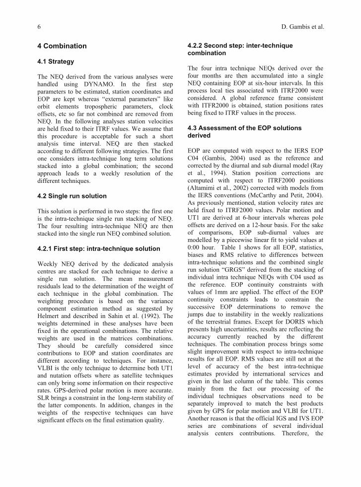
4 Combination

4.1 Strategy

The NEQ derived from the various analyses were handled using DYNAMO. In the first step parameters to be estimated, station coordinates and EOP are kept whereas “external parameters” like orbit elements tropospheric parameters, clock offsets, etc so far not combined are removed from NEQ. In the following analyses station velocities are held fixed to their ITRF values. We assume that this procedure is acceptable for such a short analysis time interval. NEQ are then stacked according to different following strategies. The first one considers intra-technique long term solutions stacked into a global combination; the second approach leads to a weekly resolution of the different techniques.

4.2 Single run solution

This solution is performed in two steps: the first one is the intra-technique single run stacking of NEQ. The four resulting intra-technique NEQ are then stacked into the single run NEQ combined solution.

4.2.1 First step: intra-technique solution

Weekly NEQ derived by the dedicated analysis centres are stacked for each technique to derive a single run solution. The mean measurement residuals lead to the determination of the weight of each technique in the global combination. The weighting procedure is based on the variance component estimation method as suggested by Helmert and described in Sahin et al. (1992). The weights determined in these analyses have been fixed in the operational combinations. The relative weights are used in the matrices combinations. They should be carefully considered since contributions to EOP and station coordinates are different according to techniques. For instance, VLBI is the only technique to determine both UT1 and nutation offsets where as satellite techniques can only bring some information on their respective rates. GPS-derived polar motion is more accurate. SLR brings a constraint in the long-term stability of the latter components. In addition, changes in the weights of the respective techniques can have significant effects on the final estimation quality.

4.2.2 Second step: inter-technique combination

The four intra technique NEQs derived over the four months are then accumulated into a single NEQ containing EOP at six-hour intervals. In this process local ties associated with ITRF2000 were considered. A global reference frame consistent with ITFR2000 is obtained, station positions rates being fixed to ITRF values in the process.

4.3 Assessment of the EOP solutions derived

EOP are computed with respect to the IERS EOP C04 (Gambis, 2004) used as the reference and corrected by the diurnal and sub diurnal model (Ray et al., 1994). Station position corrections are computed with respect to ITRF2000 positions (Altamimi et al., 2002) corrected with models from the IERS conventions (McCarthy and Petit, 2004). As previously mentioned, station velocity rates are held fixed to ITRF2000 values. Polar motion and UT1 are derived at 6-hour intervals whereas pole offsets are derived on a 12-hour basis. For the sake of comparisons, EOP sub-diurnal values are modelled by a piecewise linear fit to yield values at 0:00 hour. Table 1 shows for all EOP, statistics, biases and RMS relative to differences between intra-technique solutions and the combined single run solution “GRGS” derived from the stacking of individual intra technique NEQs with C04 used as the reference. EOP continuity constraints with values of 1mm are applied. The effect of the EOP continuity constraints leads to constrain the successive EOP determinations to remove the jumps due to instability in the weekly realizations of the terrestrial frames. Except for DORIS which presents high uncertainties, results are reflecting the accuracy currently reached by the different techniques. The combination process brings some slight improvement with respect to intra-technique results for all EOP. RMS values are still not at the level of accuracy of the best intra-technique estimates provided by international services and given in the last column of the table. This comes mainly from the fact our processing of the individual techniques observations need to be separately improved to match the best products given by GPS for polar motion and VLBI for UT1. Another reason is that the official IGS and IVS EOP series are combinations of several individual analysis centers contributions. Therefore, the

D. Gambis et al. 6

“analysis noise” is reduced and consequently the time-series becomes smoother. Table 1. Bias (first line) and RMS (second line) of the differences between single run of individual techniques solutions on one hand and long term combined inter-technique solution on the second hand with IERS C04 over the four first months of 2006. Pole components are expressed in μas, UT1 in μs.

DORIS VLBI SLR GPS COMB GRGS

Best solution

X-Pole -22 1000

-63 291

-114 193

-26 57

-17 73

(IGS) 34

Y-Pole 2000 4000

114 251

117 201

189 81

80 71

(IGS) 30

UT1 4 23 0

12 (IVS)

5

Deps -69 86 -5

62 (IVS)

55

Dψ*sinε 15 40 8

40 (IVS)

35

4.4 Inter-technique weekly solution

Another strategy is to stack the NEQ derived per technique into a global multi-technique solution. In the process local ties are applied. This is assumed to ensure the continuity between the successive weeks. In order to inverse and solve the system, constraints on EOP continuity and minimum constraints on station positions have also to be applied. Daily EOPs at 0:00 h and weekly station positions are obtained using a linear piecewise fit.

Table 2 gives the statistics concerning the two approaches, single run and weekly solutions for polar motion and UT1 differenced with C04 used as the reference. Analyses were performed applying or not EOP continuity constraints. We can note the progressive improvement of the different solutions. The weekly solution with no constraints presents significant weekly jumps which are reduced when EOP constraints are applied. The significant bias in y-pole of about 200 μas proves that the solution is expressed in a system close to ITRF, this value being the present discrepancy between ITRF and the current C04 (Gambis, 2004). The alternative procedure based on single run intra-technique combination followed by the stacking of the different NEQ is performed as well with and without applying EOP constraints. The improvement is significant. Results obtained when EOP constraints are applied are comparable to the best solutions available. It appears that local ties always applied play a different role in the two

procedures since in the case of weekly solutions, only a variable sub-set of ties is applied whose inaccuracies leads to propagate instabilities. Due to mis-modelling in the longitude of node or satellites orbits, it is well known that LOD values estimated from space satellite techniques are biased; this leads to single run errors in the integrated Universal Time UT1. The situation is similar for nutation. When calibrated by VLBI, LOD and nutation rates derived by GPS can be valuable in the combination (Gambis et al., 1993; Rothacher et al., 1999). This is apparently a difficulty in the UT1 and nutation combination as it was recently discussed by Ray et al. (2005). Still, the results we obtained show than the potential of VLBI is not degraded by the single run errors brought by GPS but it benefits from the stability of UT rates. Let us recall that VLBI intensive sessions are involved in the processing. Situation is similar for nutation. The same conclusion was given by Thaller et al. (2006). Table 2. Statistics, bias (first line) and RMS (second line) of the differences of combined weekly and long term combined inter-technique solution with and without EOP continuity constraints with IERS C04 over January-April 2006. Pole components are expressed in μas, UT1 in μs. Weekly Weekly

EOP cont Single run

Single run EOP cont

Best solution

X-Pole 1 118

-6 87

-23 114

-23 55

(IGS) 40

Y-Pole 214 123

209 99

213 119

203 74

(IGS) 40

UT1 0 10

0 10

3 10

3 10

(IVS) 5

4.5 Assessment of the quality of the global reference frame derived

Weekly sets of station coordinates are expressed in a frame consistent with the ITRF2000 used as the reference. The quality of the multi-technique combined terrestrial reference frame (GRGS) depends on the relative qualities of the contributing solutions per technique as well as on the combination strategy which is applied. The overall quality indexes of the individual solutions included in the GRGS combination is given via the transformation components. Table 3 represents the transformation between these reference frames expressed in the form of mean translation, rotation and scale factor parameters of the single run solution. It gives the accuracy of the origin and scale. We can note the significant Tx value of about 2 cm with respect to ITRF2000 which is present in


all solutions. Large translations found in the results of VLBI may result from the fact that the a-priori TRF is VTRF2005 and not ITRF2000 on contrary to other techniques. Rotation angles are negligible

as it could be expected. It appears that results concerning SLR and VLBI for the scale are significantly different from the other techniques.

Table 3. Reference frame. Mean values of the 7-parameter transformation with respect to ITRF2000 over the first four months of 2006. UNIT is cm. Standard deviations are given on second line.

Tx std

Ty std

Tz std

Scale std

Rx std

Ry std

Rz std

DORIS 2.3 0.3

0.4 0.5

-3.6 2.1

-1.9 .17

0.0 0.0

0.0 0.0

0.0 0.0

GPS 2.6 0.2

-1.3 0.4

-1.1 2.0

-1.5 0.1

1.2 0.0

-0.4 0.0

1.0 0.0

SLR 2.6 0.8

-1.8 0.7

-3.6 2.0

0.9 0.7

0.9 0.0

0.4 0.0

0.3 0.0

VLBI 1.5 0.5

-2.6 0.7

-1.2 0.6

1.1 0.5

0.0 0.0

0.3 0.0

1.0 0.0

COMBINED 2.6 0.2

-1.2 0.4

-1.1 1.2

-0.9 0.1

0.0 0.0

0.0 0.0

0.0 0.0

5 Conclusions

The combination process based on datum-free NEQ is now done on a routine basis since the beginning of 2005 in a coordinated project within the frame of GRGS. The project is still in a research phase for the processing of individual techniques as well as for the final combination. We already demonstrated the good quality of the results for EOP as well as for station coordinates. The global combined solution benefits from the mutual constraints brought by the different techniques. Better results are expected after the improvement in the processing of the individual techniques. The strength of the method is the use of a set of identical up-to-date models and standards in unique software. In addition the solution benefits from mutual constraints brought by the various techniques; UT1 and nutation offsets derived from VLBI are constrained and complemented by respectively LOD and nutation rates estimated by GPS. Before EOP and station coordinates be derived on an operational basis with an optimal accuracy different problems have to be studied and solved. EOP and station coordinate solutions are sensitive to a number of critical parameters linked to the terrestrial reference frame realization mostly local ties whose errors propagate in an unpredictable way in the station coordinates and EOP series. We are here in a context of service oriented researches. This implies that we have to find and apply the

optimal values for the critical parameters involved, minimum constraints for stations, EOP continuity constraints and techniques weights. This “tuning” is essential to provide consistent, accurate and stable products.

References

Altamimi, Z., P. Sillard, C. Boucher (2002). ITRF2000: A new Release of the International Terrestrial Reference Frame for Earth Science Applications. J. Geophys. Res. 107(B10), 2214, doi: 10.1029/2001JB000561.

Altamimi, Z., C. Boucher and D. Gambis (2005). Single run Stability of the Terrestrial Reference Frame, Adv. Space Res. 33(6): 342-349.

Andersen, PH. (2000). Multi-level arc combination with stochastic parameters. J. of Geod. 74(7-8): 531-551.

Angermann, D., H. Drewes, M. Krügel, B. Meisel, M. Gerstl, R. Kelm, H. Müller, W. Seemüller and V. Tesmer (2004). ITRS Combination Center at DGFI: A terrestrial reference frame realization 2003. Deutsche Geodätische Kommission, Reihe B, Heft Nr. 313, Munich.

D. Gambis et al. 8

Altamimi, Z., X. Collilieux, J. Legrand, B. Garayt and C. Boucher (2007). ITRF2005: A new release of the International Terrestrial Reference Frame based on time series of station positions and Earth Orientation Parameters, J. Geophys. Res., 112, B09401, doi: 10.1029/2007JB004949.

Coulot, D., P. Berio, R. Biancale, S. Loyer, L. Soudarin, A.-M. Gontier (2007). Toward a direct combination of space-geodetic techniques at the measurement level: Methodology and main issues, Journal of Geophysical Research, Vol. 112, B05410, doi:10.1029/2006JB004336.

Fey, A.L., C. Ma, E.F. Arias, P. Charlot, M. Feissel-Vernier, A.-M. Gontier, C.S. Jacobs, J. Li, D.S. MacMillan (2004). The Second Extension of the International Celestial Reference Frame: ICRF-EXT.2, Astron. J. 127, 3587-3608.

Gambis, D., N. Essaifi, E. Eisop, and M. Feissel (1993). Universal time derived from VLBI, SLR and GPS. IERS technical note 16, Dickey and Feissel (eds), ppIV15-20.

Gambis, D. (2004). Monitoring Earth Orientation at the IERS using space-geodetic observations. J. of Geodesy, 78, pp 295-303, state-of-the-art and prospective, J. of Geodesy. 78 (4-5):295-303, doi: 10.1007/s00190-004-0394-1.

Gambis, D., R. Biancale, J.-M. Lemoine, J.-C. Marty, S. Loyer, L. Soudarin, T. Carlucci, N. Capitaine, Ph. Bério, D. Coulot, P. Exertier, P. Charlot and Z. Altamimi (2006). Global combination from space geodetic techniques, Proc. Journées Systèmes de Référence 2005, Verlag des Bundesamts für Kartographie und Geodäsie, Frankfurt am Main.

Gambis, D., R. Biancale, J.-M. Lemoine, J.-C. Marty, S. Loyer, L. Soudarin, T. Carlucci, N. Capitaine, Ph. Bério, D. Coulot, P. Exertier, P. Charlot and Z. Altamimi (2007). Global combination from space geodetic techniques, in IERS Annual report for 2005, pp. 127-137 W. Dick and B. Richter (eds), BKG, 175p.

Ma, C., E.F. Arias, T.M. Eubanks, A.L. Fey, A.-M. Gontier, C.S. Jacobs, O.J. Sovers, B.A. Archinal and P. Charlot (1998). The International Celestial Reference Frame as realized by Very Long Baseline Interferometry. Astron. J. 116, 516-546.

McCarthy, D.D, G. Petit (2004). IERS Conventions 2003, IERS Technical Note No. 32.

Nothnagel, A. (2005). VTRF2005 - A combined VLBI Terrestrial Reference Frame. In: Proceedings of the 17th Working Meeting on European VLBI for Geodesy and Astrometry, pp 118-124.

Ray, R.D., D.J. Steinberg, B.F. Chao (1994). Science, 264, 830.

Ray, J., Z. Altamimi (2005). Evaluation of co-location ties relating the VLBI and GPS reference frames. J. of Geodesy 79(4-5):189-195, doi:10.1007/s00190-005-0456-z.

Ray, J., J. Kouba, Z. Altamimi (2005). Is there utility in rigorous combinations of VLBI and GPS Earth orientation parameters? J. of Geodesy 79(9):505-511, doi: 10.1007/s00190-005-0007-7.

Rothacher, M, G. Beutler, T.A. Herring, R. Weber (1999). Estimation of nutation using the Global Positioning System. J. of Geophys. Res. 104(B3):4835-4859, doi: 10.1029/1998JB900078.

Sahin, M., P.A. Cross and P.C. Sellers (1992). Bull. Géod. 66, 284.

Sillard, P. and C. Boucher (2001). Review of algebraic constraints in terrestrial reference frame datum definition. J. of Geodesy 75, 63-73.

Thaller, D., M. Krügel, M. Rothacher, V. Tesmer, R. Schmid and D. Angermann (2007). Combined Earth Orientation Parameters based on Homogeneous and Continuous VLBI and GPS data, J. of Geodesy, Volume 81, Issue 6-8, pp.529-541.

Yaya, Ph. (2002). Apport des combinaisons de techniques astrométriques et géodésiques à l’estimation des paramètres d’orientation de la terre. PhD thesis, Observatoire de Paris


DGFI Combination Methodology for ITRF2005 Computation


D. Angermann et al. 12

Accumulation of time series normal equations

Localties Inter - technique combination

ITRF 2005 solutionTRF (x, v) + EOP

VLBIMulti-year NEQTRF(x, v) + EOP

SLRMulti-year NEQTRF(x, v) + EOP

GPSMulti-year NEQTRF(x, v) + EOP

DORISMulti-year NEQTRF(x, v) + EOP

VLBI SLR GPS DORIS

NEQ sess. 1

NEQ sess. 2

NEQ sess. nPositions + EOP

NEQ week 1

NEQ week 2

NEQ week nPositions + EOP



NEQ week 1

NEQ week 2

NEQ week 1

NEQ week 2

82.58

82.6

82.62

82.64

82.66

82.68

82.7

82.72

−1000 −500 0 500 1000 1500 2000

Hei

ght [

m]

Time [jd2000]

82.58

82.6

82.62

82.64

82.66

82.68

82.7

82.72

−1000 −500 0 500 1000 1500 2000

Hei

ght [

m]

Time [jd2000]

82.58

82.6

82.62

82.64

82.66

82.68

82.7

82.72

−1000 −500 0 500 1000 1500 2000

Hei

ght [

m]

Time [jd2000]

DGFI Combination Methodology for ITRF2005 Computation 13

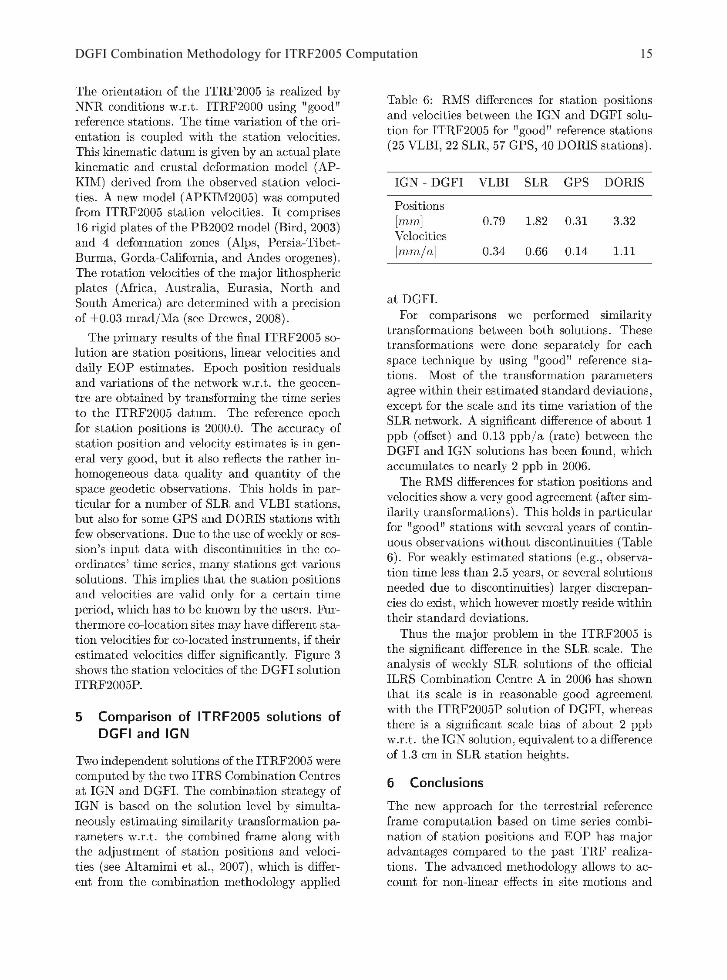
DGFI Combination Methodology for ITRF2005 Computation 15

180˚ -120˚ -60˚ 0˚ 60˚ 120˚ 180˚

-60˚-60˚

0˚0˚

60˚60˚

4 cm/a ITRF2005P (DGFI)


D. THALLER, M. ROTHACHER GeoForschungsZentrum Potsdam (GFZ), Telegrafenberg, 14473 Potsdam, Germany

M. KRÜGEL Deutsches Geodätisches Forschungsinstitut (DGFI), Alfons-Goppel-Straße 11, 80539 München, Germany

Email: [email protected] Phone: ++49-331-288-1880 Fax: ++49-331-288-1759

Abstract. The parameter space that can be covered by GPS, VLBI and SLR is very broad, and many overlaps exist between the techniques. Up to now, this is not yet fully exploited in inter-technique com-parisons and combinations as in most cases only station positions and Earth orientation parameters (EOP) are considered. In this contribution we include the troposphere parameters additionally, and it is demonstrated that a combined terrestrial reference frame (TRF) improves the agreement of the GPS- and VLBI-derived troposphere zenith delays (ZD). The benefit of a combination is shown for the EOP as well, although non-continuous VLBI observations complicate the situation for Universal Time (UT). Finally, the potential of connecting GPS and SLR by estimating degree one spherical harmonic coeffi-cients of the Earth’s gravity field is analyzed.

Keywords: EOP, troposphere parameters, low-degree spherical harmonics, rigorous combination ___________________________________

1 Introduction

Many solutions from the space-geodetic techniques are available through the International Earth Rotation and Reference Systems Service (IERS) and its tech-nique-specific services. However, in most cases the provided time series show systematic biases and reveal differences that result from the application of different models during the analyses of the observa-tions. In order to give one example, Schmid et al. (2005) demonstrated that the usage of phase centre models for GPS antennas that were calibrated rela-tively to one reference antenna instead of absolutely calibrated models causes significant biases in the ZD of several millimetres. All differences in the a priori models that were used to generate solutions show up as discrepancies in the estimated parameters. In order to overcome this problem, GeoForschungsZentrum Potsdam, Deutsches Geodätisches Forschungsinstitut,

Institute for Geodesy and Geoinformation of the University of Bonn and Bundesamt für Kartographie und Geodäsie joined forces. Within this group, a broad variety of expertise concerning the analysis of GPS, VLBI and SLR is available so that high-quality solutions for all of these techniques could be gener-ated. The alignment of the analysis standards within the group goes considerably beyond the IERS Con-ventions 2003 (McCarthy and Petit 2004) and their updates, as detailed agreements were made concern-ing the models used for, e.g., pole tide, ocean load-ing, a priori ZD delay, mapping function for the tro-posphere delay, a priori nutation, or the method of interpolating the a priori EOP to the epochs of obser-vation.

2 Analysis strategy

2.1 Processing procedure

The analysis can be divided into four major steps:

- analysis of the observations for the year 2004 using the pre-defined common standards to get single-technique normal equations (NEQs),

- generation of yearly single-technique solutions,

- generation of weekly combined NEQs,

- generation of a yearly solution based on the weekly combined NEQs of the preceding step.

The full reprocessing of all observations (step 1) delivers homogeneous time series for each technique. The GPS analysis was done with the Bernese GPS Software 5.0 (Dach et al. 2007), EPOS at GFZ was used for the SLR analysis, and two VLBI solutions computed with CalcSolve (Petrov 2002) and Occam (Titov et al. 2004) have been combined to an intra-technique VLBI solution according to Vennebusch et al. (2007). It must be emphasized that the application of common analysis standards in all these software packages guarantees a high level of homogeneity

Combining One Year of Homogeneously Processed GPS, VLBI and SLR Data


between the techniques, although the homogenization can still be improved. Another important advantage of our studies is the extended parameter space. Nor-mally, just station coordinates and EOP are provided in the solutions available via the IERS. We included additionally station-specific troposphere parameters (ZD and horizontal gradients) for GPS and VLBI, geocentre coordinates for GPS, and spherical har-monic coefficients (SH) of the Earth’s gravity field for SLR (degree 1-2). Amongst others, Pavlis (2004) showed that the estimation of low-degree SH from SLR observations is reasonable. The datum-free NEQs resulting from step 1 cover one week in the case of GPS and SLR, and 24 hours in the case of VLBI, where 129 global and eight regional sessions were selected. The regional sessions do not allow a reasonable estimation of EOP, but they deliver a valuable densification for the TRF.

Yearly single-technique solutions were generated in the second step. This step is necessary to get an idea about the potential of each technique and, thus, to realistically assess the quality that can be expected for the combined solution. An internal measure for the quality of the solutions is the repeatability of station coordinates (Table 1). The quite dense net-work of almost 200 GPS sites reveals the best stabil-ity with a weekly repeatability of about 2 mm for the horizontal components and a factor three worse for the height. Correlations of the height with the tropo-sphere delay and the clocks are responsible for the worse stability compared to the horizontal compo-nents. This behaviour is visible for the VLBI solution as well, but its repeatability is worse by a factor of about two compared to GPS. However, it must be kept in mind that the VLBI network is less dense and determined with 24-hour sessions. SLR, with the same amount of stations but weekly solutions, is less precise than VLBI. Considering that we have a single SLR solution and that all sites contribute to the re-peatabilities, the order of magnitude agrees well within that shown by Bianco et al. (2006). Compar-ing with other analysis (e.g. Altamimi et al. 2007), it must be emphasized that we use an RMS instead of WRMS, and internal comparisons showed that this difference is especially important for VLBI and SLR where the formal errors are strongly varying. The 3D repeatabilities were used for a relative weighting of the technique-specific NEQs in the combination.

Finally, a yearly solution based on the previously generated weekly combined NEQ was computed in order to have a homogeneous TRF as basis for the time series of EOP and troposphere parameters. The TRF datum has been defined by a sub-set of good GPS sites using a no-net-rotation and no-net-translation condition w.r.t. ITRF2000 (Altamimi

e SH of degree one from SLR data, SLR itself cannot contribute to the transla-tional datum. The SH of degree one and the geocen-ter coordinates from SLR and GPS, respectively, are not combined as we first want to analyze the esti-mates regarding any systematic differences.

The connection between the three techniques’ networks was realized by the application of local ties (LT) at co-located sites. An overview of the co-locations available for our analysis is given in Fig. 1 (at the end). Altogether there are 30 VLBI-GPS co-locations, 23 SLR-GPS co-locations and therein six stations where all three techniques are assembled. Unfortunately, no further VLBI-SLR co-locations are available so that these networks are connected mainly indirectly via GPS. After a careful selection, we applied LT for 23 VLBI-GPS and 21 SLR-GPS co-locations.

Table 1: Repeatability of station coordinates for the single-technique solutions in [mm]. Solution #Stations North East Up 3D GPS (week) 185 1.91 1.80 5.66 3.60 VLBI (day) 33 4.65 4.00 11.09 7.32

SLR (week) 32 15.61 17.16 17.13 16.65

2.2 Combination strategy for EOP

It is essential to say some words about the parame-terization and the combination strategy for EOP to understand and interpret the results. Figure 2 visual-izes the basic principle. The difficulty in combining daily EOP from satellite techniques and VLBI is due to the data coverage: GPS and SLR observe continu-ously whereas gaps occur between two consecutive 24 h VLBI sessions so that a continuous time series at daily intervals cannot be derived. An additional problem arises because VLBI sessions typically start at 17 or 18 UTC. Thus, the balance point of all ob-servations, where offset and drift parameters are estimated best, differs from 12 UTC. We deal with this situation in such a way that we change the parameterization in the NEQs from offset/drift per session into a linear function with two values at 0 and 24 UTC (“polygon 0h-0h”) which can then be stacked with the appropriate midnight epochs of the piece-wise linear parameterization used for the con-tinuous time series (“continuous polygon”) derived from GPS and SLR. It is clear that a VLBI-only time series consisting of offsets given at the mid-epochs of the sessions is more stable than a time series of esti-mates at 0 h. Thus, if the best VLBI-only estimates are of interest, the EOP offsets at the mid-epochs of the sessions should be considered. However, if we

D. Thaller et al. 18

et al. 2002). As we estimate th

want to realistically assess the contribution of each technique to the combined time series, we must look at the parameterization as a polygon, especially in cases where the contribution of VLBI is essential, i.e., UT1-UTC and the nutation angles.

Fig. 2: Combination strategy for time series of daily parame-ters derived from continuous and session-wise data.

3 Analyses results

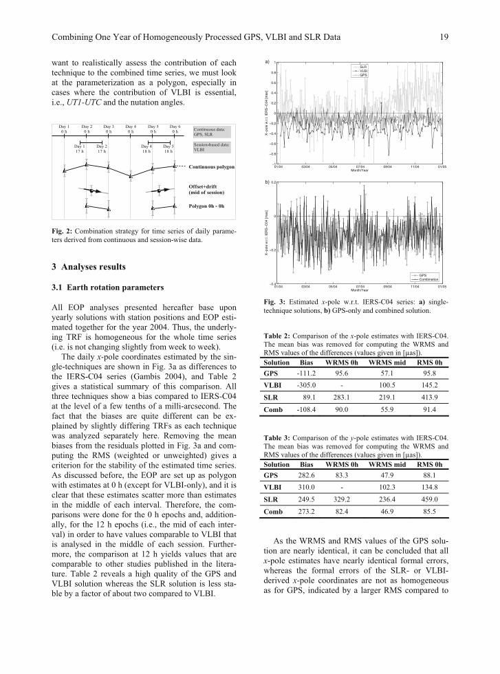
3.1 Earth rotation parameters

All EOP analyses presented hereafter base upon yearly solutions with station positions and EOP esti-mated together for the year 2004. Thus, the underly-ing TRF is homogeneous for the whole time series (i.e. is not changing slightly from week to week).

The daily x-pole coordinates estimated by the sin-gle-techniques are shown in Fig. 3a as differences to the IERS-C04 series (Gambis 2004), and Table 2 gives a statistical summary of this comparison. All three techniques show a bias compared to IERS-C04 at the level of a few tenths of a milli-arcsecond. The fact that the biases are quite different can be ex-plained by slightly differing TRFs as each technique was analyzed separately here. Removing the mean biases from the residuals plotted in Fig. 3a and com-puting the RMS (weighted or unweighted) gives a criterion for the stability of the estimated time series. As discussed before, the EOP are set up as polygon with estimates at 0 h (except for VLBI-only), and it is clear that these estimates scatter more than estimates in the middle of each interval. Therefore, the com-parisons were done for the 0 h epochs and, addition-ally, for the 12 h epochs (i.e., the mid of each inter-val) in order to have values comparable to VLBI that is analysed in the middle of each session. Further-more, the comparison at 12 h yields values that are comparable to other studies published in the litera-ture. Table 2 reveals a high quality of the GPS and VLBI solution whereas the SLR solution is less sta-ble by a factor of about two compared to VLBI.

01/04 03/04 05/04 07/04 09/04 11/04 01/05−1

−0.8

−0.6

−0.4

−0.2

0

0.2

0.4

0.6

0.8

1

Month/Year

X−

pole

w.r

.t. IE

RS

−C

04 [m

as]

SLRVLBIGPS

a)

01/04 03/04 05/04 07/04 09/04 11/04 01/05−0.4

−0.2

0

0.2

Month/Year

X−

pole

w.r

.t. IE

RS

−C

04 [m

as]

GPSCombination

b)

Fig. 3: Estimated x-pole w.r.t. IERS-C04 series: a) single-technique solutions, b) GPS-only and combined solution.

Table 2: Comparison of the x-pole estimates with IERS-C04. The mean bias was removed for computing the WRMS and RMS values of the differences (values given in [μas]). Solution Bias WRMS 0h WRMS mid RMS 0h GPS -111.2 95.6 57.1 95.8 VLBI -305.0 - 100.5 145.2

SLR 89.1 283.1 219.1 413.9

Comb -108.4 90.0 55.9 91.4

Table 3: Comparison of the y-pole estimates with IERS-C04. The mean bias was removed for computing the WRMS and RMS values of the differences (values given in [μas]). Solution Bias WRMS 0h WRMS mid RMS 0h GPS 282.6 83.3 47.9 88.1

VLBI 310.0 - 102.3 134.8

SLR 249.5 329.2 236.4 459.0

Comb 273.2 82.4 46.9 85.5

As the WRMS and RMS values of the GPS solu-tion are nearly identical, it can be concluded that all x-pole estimates have nearly identical formal errors, whereas the formal errors of the SLR- or VLBI-derived x-pole coordinates are not as homogeneous as for GPS, indicated by a larger RMS compared to

Combining One Year of Homogeneously Processed GPS, VLBI and SLR Data 19

the WRMS. The scatter in the x-pole is slightly im-proved in the combined solution (Table 2, Fig. 3b).

The analysis of the y-pole shows similar results concerning the WRMS (Table 3). Contrary to the x-pole, the y-pole estimates of all solutions are biased similarly compared to IERS-C04 by about 0.25 to 0.3 mas. This large bias is caused by inconsistencies between ITRF2000 and the IERS-C04 series, and it clearly points out that IERS-C04 cannot be consid-ered to be the truth.

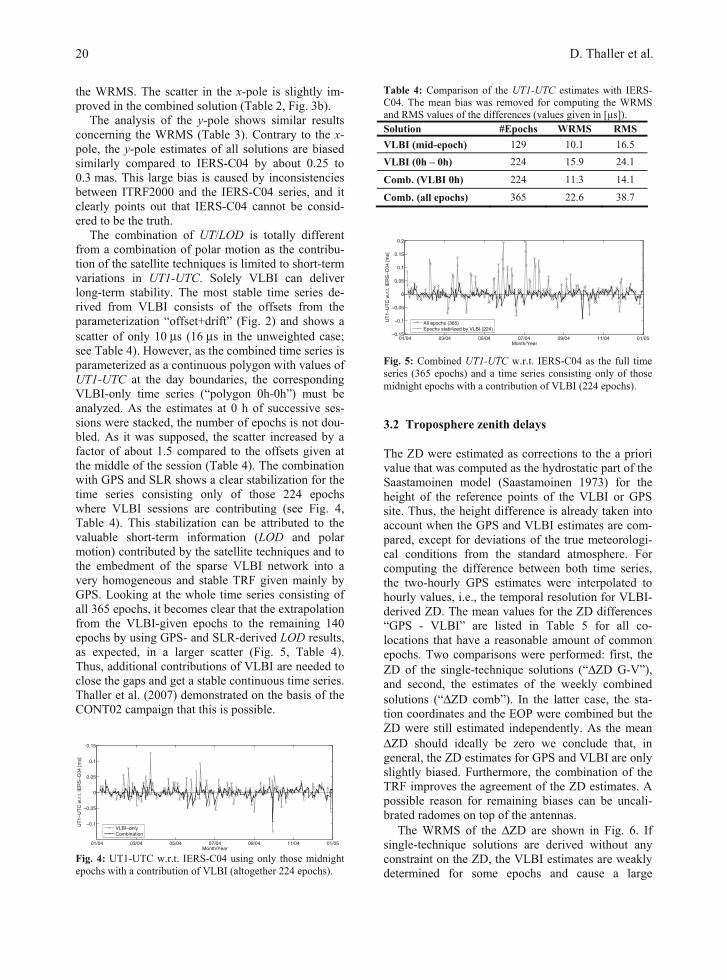
The combination of UT/LOD is totally different from a combination of polar motion as the contribu-tion of the satellite techniques is limited to short-term variations in UT1-UTC. Solely VLBI can deliver long-term stability. The most stable time series de-rived from VLBI consists of the offsets from the parameterization “offset+drift” (Fig. 2) and shows a scatter of only 10 μs (16 μs in the unweighted case; see Table 4). However, as the combined time series is parameterized as a continuous polygon with values of UT1-UTC at the day boundaries, the corresponding VLBI-only time series (“polygon 0h-0h”) must be analyzed. As the estimates at 0 h of successive ses-sions were stacked, the number of epochs is not dou-bled. As it was supposed, the scatter increased by a factor of about 1.5 compared to the offsets given at the middle of the session (Table 4). The combination with GPS and SLR shows a clear stabilization for the time series consisting only of those 224 epochs where VLBI sessions are contributing (see Fig. 4, Table 4). This stabilization can be attributed to the valuable short-term information (LOD and polar motion) contributed by the satellite techniques and to the embedment of the sparse VLBI network into a very homogeneous and stable TRF given mainly by GPS. Looking at the whole time series consisting of all 365 epochs, it becomes clear that the extrapolation from the VLBI-given epochs to the remaining 140 epochs by using GPS- and SLR-derived LOD results, as expected, in a larger scatter (Fig. 5, Table 4). Thus, additional contributions of VLBI are needed to close the gaps and get a stable continuous time series. Thaller et al. (2007) demonstrated on the basis of the CONT02 campaign that this is possible.

01/04 03/04 05/04 07/04 09/04 11/04 01/05

−0.1

−0.05

0

0.05

0.1

0.15

Month/Year

UT

1−U

TC

w.r

.t. IE

RS

−C

04 [m

s]

VLBI−onlyCombination

Fig. 4: UT1-UTC w.r.t. IERS-C04 using only those midnight epochs with a contribution of VLBI (altogether 224 epochs).

Table 4: Comparison of the UT1-UTC estimates with IERS-C04. The mean bias was removed for computing the WRMS and RMS values of the differences (values given in [μs]). Solution #Epochs WRMS RMS VLBI (mid-epoch) 129 10.1 16.5 VLBI (0h – 0h) 224 15.9 24.1

Comb. (VLBI 0h) 224 11.3 14.1

Comb. (all epochs) 365 22.6 38.7

01/04 03/04 05/04 07/04 09/04 11/04 01/05−0.15

−0.1

−0.05

0

0.05

0.1

0.15

0.2

Month/Year

UT

1−U

TC

w.r

.t. IE

RS

−C

04 [m

s]

All epochs (365)Epochs stabilized by VLBI (224)

Fig. 5: Combined UT1-UTC w.r.t. IERS-C04 as the full time series (365 epochs) and a time series consisting only of those midnight epochs with a contribution of VLBI (224 epochs).

3.2 Troposphere zenith delays

The ZD were estimated as corrections to the a priori value that was computed as the hydrostatic part of the Saastamoinen model (Saastamoinen 1973) for the height of the reference points of the VLBI or GPS site. Thus, the height difference is already taken into account when the GPS and VLBI estimates are com-pared, except for deviations of the true meteorologi-cal conditions from the standard atmosphere. For computing the difference between both time series, the two-hourly GPS estimates were interpolated to hourly values, i.e., the temporal resolution for VLBI-derived ZD. The mean values for the ZD differences “GPS - VLBI” are listed in Table 5 for all co-locations that have a reasonable amount of common epochs. Two comparisons were performed: first, the ZD of the single-technique solutions (“ΔZD G-V”), and second, the estimates of the weekly combined solutions (“ΔZD comb”). In the latter case, the sta-tion coordinates and the EOP were combined but the ZD were still estimated independently. As the mean ΔZD should ideally be zero we conclude that, in general, the ZD estimates for GPS and VLBI are only slightly biased. Furthermore, the combination of the TRF improves the agreement of the ZD estimates. A possible reason for remaining biases can be uncali-brated radomes on top of the antennas.

The WRMS of the ΔZD are shown in Fig. 6. If single-technique solutions are derived without any constraint on the ZD, the VLBI estimates are weakly determined for some epochs and cause a large


WRMS. This problem can be remedied if the ZD of successive epochs are slightly constrained (1 m in our case), although the constraint is not necessary for most of the stations, thus, it does not influence their ZD estimates. The positive effect of the combination can be seen in significantly reduced WRMS for those stations where the VLBI time series needs some stabilization. Thus, the stable TRF of GPS can help to stabilize the ZD for the VLBI site, although this effect is not as large as a constraint directly on the ZD, of course. However, the WRMS slightly in-creases in the combination compared to the single-techniques if additional constraints are applied. But in general, the scatter of the ZD biases is only a few millimetres indicating an overall good agreement. The results agree well with the comparisons done by Steigenberger et al. (2007), although their analysis covers a much longer time span.

0

5

10

15

20

25

30

HOB2

MEDI

ONSA

TSK2

TSKB

HRAO

FORT

ALGO

CONZ

WES2

NYA1

KOKB

NYAL

FAIR

WTZR

WR

MS

of Δ

ZD

[mm

]

Single−techn. w/o constraintsSingle−techn. + rel. constraintsCombination w/o constraintsCombination + rel. constraints

Fig. 6: WRMS of the differences between the ZD estimates for GPS and VLBI sites. The biases (Table 5) were removed.

3.3 Geocentre coordinates

Concerning the spherical harmonic coefficients SHnm of degree n and order m, the paper concentrates on the coefficients of degree 1 as they are related to the geocentre coordinates Xgcc:

nmnmgcc RH SHX ⋅⋅= (1)

with the normalization factor Hnm, which is 3 in the case of n=1, and the radius of the Earth R. The SH estimated by SLR were converted into coordi-nates of the geocentre according to Eq. 1 and then compared to the GPS estimates (see Fig. 7). At a first glance, there are only a few similarities in the tempo-ral behaviour of both time series and in y-direction there is even a bias of about 1 cm which is assumed to be caused by orbit modelling deficiencies in the GPS solution. As expected, the z-component is de-termined more stably by SLR than by GPS, so that the solution benefits from a combination. For the other components the scatter is nearly identical for both techniques, i.e., about 4 mm.

01/04 03/04 05/04 07/04 09/04 11/04 01/05−0.025

−0.02

−0.015

−0.01

−0.005

0

0.005

0.01

Month/Year

X−G

CC

[m]

SLR: C11GPS: X−GCC

01/04 03/04 05/04 07/04 09/04 11/04 01/05−0.01

−0.005

0

0.005

0.01

0.015

0.02

0.025

Month/Year

Y−G

CC

[m]

SLR: S11GPS: Y−GCC

01/04 03/04 05/04 07/04 09/04 11/04 01/05−0.06

−0.04

−0.02

0

0.02

0.04

Month/Year

Z−G

CC

[m]

SLR: C10GPS: Z−GCC

Fig. 7: Geocentre coordinates from GPS and corresponding SH of degree 1 from SLR converted to geocentre coordinates.

4 Conclusions and outlook

For the first time, homogeneous contributions of GPS, VLBI and SLR were combined for one year including station positions, EOP, troposphere pa-rameters and low-degree SH of the geopotential.

The benefit of a combination was shown for the ZD, as a homogeneous TRF (from GPS) increases the agreement between GPS and VLBI estimates and gives stabilization for weakly determined epochs. The next step will be the combination of the tropo-sphere parameters which was already proven to be successful by Krügel et al. (2007) for the CONT02 campaign.

It was shown that not only the pole coordinates benefit from a combination, but the time series of UT1-UTC as well. However, the problem with gaps between the 24 h sessions of VLBI remains, and it has to be investigated whether the “Intensive” VLBI sessions can help as they deliver UT almost daily.

The inclusion of SH of the geopotential gives an additional link between the techniques, although the potential of a combination still has to be ascertained.

Moreover, in the future, the correlations between the various parameter types will be studied in detail.

Acknowledgements. The funding for most of this work is granted by the German Bundesministerium für Bildung und Forschung (BMBF) within the

Combining One Year of Homogeneously Processed GPS, VLBI and SLR Data 21

Geotechnologien project 03F0425A and we like to thank all colleagues contributing to this project.

References

Altamimi Z, Sillard P, Boucher C (2002) ITRF2000: A new Release of the International Terrestrial Reference Frame for Earth Science Applications. J Geophys Res 107(B19)

Altamimi Z, Collilieux X, Legrand J, Garayt B, Boucher C (2007) ITRF2005 : A new release of the International Ter-restrial Reference Frame based on time series of station po-sitions and Earth Orientation Parameters. J Geophys Res 112, B09401

Bianco G, Luceri V, Sciaretta C (2006) The ILRS Standard Products : a quality assessment. 15th International Work-shop on Laser Ranging, Canberra, October 15-20, 2006

Gambis D (2004) Monitoring Earth orientation using space-geodetic techniques : state-of-the-art and perspective. J Geod 78(4-5):295-303.

Dach R, Hugentobler U, Fridez P, Meindl M (eds.) (2007) Bernese GPS Software Version 5.0, Astronomical Institute, University of Berne, Switzerland.

Krügel M, Thaller D, Tesmer V, Rothacher M, Angermann D, Schmid R (2007) Tropospheric parameters: Combination studies based on homogeneous VLBI and GPS data. J Geod 81(6-8):515-527

McCarthy DD, Petit G (2004) IERS Conventions 2003. IERS Technical Note No. 32, Verlag des Bundesamts für Karto-graphie und Geodäsie, Frankfurt am Main, Germany.

Pavlis EC (2004) SLR contributions in the establishment of the terrestrial reference frame. Proceedings of the 14th Interna-tional Workshop on Laser Ranging, San Fernando, June 7-11, 2004

Petrov L (2002) Mark IV VLBI analysis software Calc/Solve. Web document : http://gemini.gsfc.nasa.gov/solve

Saastamoinen J (1973) Contributions to the theory of atmos-pheric refraction. Bull Géod, 107: 13-34.

Schmid R, Rothacher M, Thaller D, Steigenberger P (2005) Absolute phase center corrections of satellite and receiver antennas: Impact on global GPS solutions and estimation of azimuthal phase center variations of the satellite antenna. GPS Solutions 9(4):283-293.

Steigenberger P, Tesmer V, Krügel M, Thaller D, Schmid R, Vey S, Rothacher M (2007) Comparisons of homogeneou-sly reprocessed GPS and VLBI long time-series of tropos-phere zenith delays and gradients. J Geod 81(6-8):503-514

Titov O, Tesmer V, Böhm J (2004) OCCAM V6.0 software for VLBI data analysis. In: Vandenberg N, Baver K (eds) IVS 2004 General Meeting Proceedings. NASA/CP-2004-212255

Thaller D, Krügel M, Rothacher M, Tesmer V, Schmid R, Angermann D (2007) Combined Earth Orientation Parame-ters based on Homogeneous and Continuous VLBI and GPS data. J Geod 81(6-8):529-541

Vennebusch M, Böckmann S, Nothnagel A (2007) The contri-bution of Very Long Baseline Interferometry to ITRF2005. J Geod 81(6-8):553-564

Fig. 1: Network of co-located sites for the year 2004.

Table 5: Mean difference of the ZD estimates derived from single-technique solutions (“G-V”) and the combined solution (“comb”), given as GPS – VLBI in mm. The height difference between the reference points has been taken into account. Station hob2 medi onsa tsk2 tskb hrao fort algo conz wes2 nya1 kokb nyal fair wtzr #Epochs 594 658 683 818 818 1029 1260 1366 1376 1552 1589 1652 1677 2228 2784

ΔZD G-V -0.9 -1.5 -1.3 -0.3 -1.2 -3.1 13.4 1.6 -1.6 4.2 -0.9 -1.1 -2.2 -3.5 -0.6

ΔZD comb 1.4 -3.3 -2.3 0.1 -0.3 0.9 4.9 0.7 -1.2 4.6 -0.1 -1.0 0.6 -3.2 -0.1


international association of geodesy...

Documents