interference coordination for femtocell networks -...
TRANSCRIPT
Interference Coordination forFemtocell Networks
Vom Promotionsausschuss derTechnischen Universitat Hamburg-Harburgzur Erlangung des akademischen Grades
Doktor-Ingenieur (Dr.-Ing.)genehmigte Dissertation
vonSerkan Uygungelen
ausAdana, Turkei
2015
1. Gutachter: Prof. Dr.-Ing. Gerhard Bauch
2. Gutachter: Prof. Dr. Harald Haas
Tag der mundlichen Prufung: 25. August 2015
ii
Abstract
Data traffic has dramatically increased in wireless cellular networks in recent times, thanks to
various video services and high-speed mobile access of smart phones. Countering such a dra-
matic traffic increase has become one of the major issues for network operators. In order to
meet the boosted data demand, novel techniques such as orthogonal frequency division multi-
ple access (OFDMA) and multiple-input and multiple-output (MIMO) are developed for next
generation mobile networks. Nevertheless, by just improving the transmission techniques and
developing advanced receivers and transmitters, the desired system requirements cannot be sat-
isfied. It is also essential to increase the radio resources used for transmission. This can simply
be done by using a wider spectrum; however, the spectrum itself is a rare and expensive re-
source. An alternative way is to increase the spatial reuse of resources through decreasing cell
sizes, which is applied by operators for a long time. On the other hand, due to the high opera-
tion and infrastructure costs of base stations (BSs), operators are reluctant to dense deployment
of BSs. One solution to this problem is the introduction of femto-BSs, also known as home
evolved NodeB (HeNB). These are low-power and small scale BSs that are deployed within
traditional macro-cellular networks. With these so-called small cells, the spatial reuse of radio
resources is tremendously boosted. Additionally, femto-BSs can be deployed by end users in
their own premises. By deploying such small cells indoors, wall penetration losses are largely
mitigated, and users can enjoy high data rates.
In addition to its various advantages, the deployment of femtocells also comes with some prob-
lems. One of the main issues is the increase in interference. Unlike macrocell networks, fem-
tocell networks are typically randomly deployed without sophisticated planning of the network
topology. This causes high co-channel interference between cells, especially in networks where
iii
Abstract
the BSs are densely deployed, such as within public buildings or residential apartment com-
plexes.
The interference mitigation in femtocell networks is the main aim of this thesis. In order to
achieve this goal, the characteristics and interference environment of femtocell deployments
have been investigated, and the properties of interference mitigation techniques applicable to
such networks are studied. It has been shown that conventional techniques used for macro-
cell networks are not applicable for such uncoordinated networks. To this end, dynamic re-
source partitioning methods have been developed where network can update itself depending
on the changes in the interference environment. Central and distributed resource assignment
approaches have been investigated and compared. For this purpose, extensive simulations with
different scenarios have been carried out to see the overall picture clearly. Furthermore, the
application of the developed techniques in real network deployments such as Long-Term Evo-
lution (LTE) and Long-Term Evolution-Advanced (LTE-A) have been studied. Although the
focus is on femtocell networks, the developed methods in this thesis can be applied to any
wireless networks with minor changes.
As a final remark, some parts of this thesis are already published in the Institute of Electrical
and Electronics Engineers (IEEE) conferences that can be found in the Publications Section of
the thesis.
iv
Zusammenfassung
Durch die erhohte Nutzung von Videodiensten und datenintensiven Zugriffen durch Smart-
phones ist das Datenaufkommen in Drahtlosnetzwerken in den letzten Jahren drastisch gestiegen.
Diesem Anstieg zu begegnen ist eine der Hauptaufgaben fur Netzwerkbetreiber geworden. Um
die erhohte Nachfrage zu bedienen, werden neue Techniken wie OFDMA und MIMO fur die
nachste Generation von Mobilfunknetzen entwickelt. Jedoch konnen trotz der Verbesserung
von Ubertragungstechniken und der Entwicklung neuer Sender und Empfanger die gewunschten
Anforderungen nicht erfullt werden. Es ist zusatzlich wesentlich, die Ubertragungsressourcen
zu vermehren. Dies kann durch eine Verbreiterung des Spektrums erreicht werden. Jedoch ist
das Spektrum rar und teuer. Eine Alternative dazu ist die Erhohung der raumlichen Wiederver-
wendung durch kleinere Zellengroßen, welche von Netzbetreibern schon lange durchgefuhrt
wird. Allerdings zogern Betreiber vor dieser Methode, da die Kosten fur Betrieb und Infras-
truktur fur Basisstationen sehr hoch sind. Eine Losung zu diesem Problem ist die Einfuhrung
von Femtobasisstationen, die auch als Home Evolved NodeB bekannt sind. Dies sind kleine
Basisstationen mit niedriger Sendeleistung, welche innerhalb des traditionellen Makronetzw-
erkes eingesetzt werden. Mit diesen Kleinzellen wird die raumliche Wiederverwendung der
Ubertragungsressourcen enorm gesteigert. Femtobasisstationen konnen von Endnutzern in
ihren eigenen Raumlichkeiten installiert werden. Durch diesen Einsatz konnen Wanddurch-
dringungsverluste stark abgeschwacht und hohere Datenraten erreicht werden.
Allerdings erzeugen Femtobasisstationen auch Herausforderungen. Die großte Herausforderung
ist dabei die gesteigerte Interferenz. Anders als bei Makrozellen sind Femtobasisstationen
typischerweise zufallig verteilt, ohne anspruchsvolle Planung der Netzwerktopologie. Dies
fuhrt zu hoher Gleichkanalinterferenz zwischen den Zellen, besonders in Netzwerken mit hoher
v
Zusammenfassung
Dichte von Basisstationen, wie zum Beispiel in offentlichen Gebauden oder Wohnkomplexen.
Die Abschwachung von Interferenz in Femtobasisstationsnetzwerken ist das Ziel dieser Ar-
beit. Um dieses Ziel zu erreichen, wurden die Charakteristiken und die Interferenzumge-
bung von Femtozellen erforscht und die Eigenschaften von fur solche Netze geeigneten In-
terferenzschwachungstechniken studiert. Es wurde gezeigt, dass konventionelle Techniken fur
Makrozellen in unkoordinierten Netzen nicht geeignet sind. Daher wurden Methoden zur dy-
namischen Ressourcenverteilung entwickelt, durch welche sich das Netzwerk selbststandig ak-
tualisieren kann, abhangig von der Interferenzsituation. Ansatze zur zentralen und zur verteilten
Ressourcenverteilung wurden erforscht und verglichen. Zu diesem Zweck wurden umfassende
Simulationen in verschiedenen Szenarien durchgefuhrt, die einen Uberblick ermoglichen. Zusatz-
lich wurden die vorgeschlagenen Techniken in aktuellen Standards wie LTE und LTE-A getestet.
Obwohl der Fokus hier auf Femtonetzwerken liegt, konnen die entwickelten Methoden mit
kleinen Anpassungen auch in anderen Drahtlosnetzwerken eingesetzt werden.
Anmerkung: Teile dieser Arbeit wurden auf IEEE-Konferenzen veroffentlicht. Details konnen
in dem Kapitel Veroffentlichungen (Publications Section) entnommen werden.
vi
Acknowledgments
First and foremost, I would like to thank Prof. Gerhard Bauch for his supervision throughout
my work. I appreciate all his time, aspiring guidance and invaluably constructive criticism. I
am also grateful to my manager Gunther Auer in DOCOMO Euro-Labs for guiding me with
his deep experience and knowledge to build the thesis from the beginning. Furthermore, I am
thankful to Prof. Harald Haas for being my thesis examiner.
It was my privilege to have worked closely with my colleagues at DOCOMO Euro-Labs.
Firstly, I thank to Zubin Bharucha for his great and invaluable support during my thesis. I am
also grateful to Hauke Holtkamp for his help, especially with the German language. I had many
useful discussions and entertaining moments with my office-mates Samer Bazzi and Thorsten
Biermann, I thank both of them. Also, I would like to thank Hidekazu Taoka, Guido Dietl,
Emmanuel Ternon, Katsutoshi Kusume, Petra Weitkemper, Marwa El Hefnawy and all other
colleagues and friends from DOCOMO Euro-Labs. They made my time at DOCOMO Euro-
Labs a valuable and unforgettable experience. I express my warm thanks to BeFemto project
team members for their contribution to my work. Furthermore, I am indebted to my sister-in-
law Ayse Cochet and her husband Sebastien Cochet for their great support and encouragement
especially for helping me with language issues and sharing their experiences.
Special thanks to my family. Despite the distance between us, I knew that they were always
there for me and they always supported me in every decision I took. Last but obviously not
least, I want to thank deeply to my lovely wife Dilek. She is the one who encouraged me from
the very beginning to the end of my PhD work. She was always with me and gave her support
in all aspects whenever I need any help.
vii

Acknowledgments
viii
Contents
Abstract . . . . . . . . . . . . . . . . . . . . . . . . . . . . . . . . . . . . . . iiiZusammenfassung . . . . . . . . . . . . . . . . . . . . . . . . . . . . . . . . vAcknowledgments . . . . . . . . . . . . . . . . . . . . . . . . . . . . . . . . viiContents . . . . . . . . . . . . . . . . . . . . . . . . . . . . . . . . . . . . . . viiiList of Figures . . . . . . . . . . . . . . . . . . . . . . . . . . . . . . . . . . . xiiiList of Tables . . . . . . . . . . . . . . . . . . . . . . . . . . . . . . . . . . . xixAcronyms and Abbreviations . . . . . . . . . . . . . . . . . . . . . . . . . . . xxiNomenclature . . . . . . . . . . . . . . . . . . . . . . . . . . . . . . . . . . . xxvii
1 Introduction 1
2 Background and Motivation 52.1 Achieving High Data Rates in Wireless Networks . . . . . . . . . . . . . . . . 52.2 Basic Concepts of Cellular Networks . . . . . . . . . . . . . . . . . . . . . . . 9
2.2.1 Overview . . . . . . . . . . . . . . . . . . . . . . . . . . . . . . . . . 92.2.2 Duplexing Techniques . . . . . . . . . . . . . . . . . . . . . . . . . . 102.2.3 Multiple Access Methods . . . . . . . . . . . . . . . . . . . . . . . . 112.2.4 Multi-User Scheduling . . . . . . . . . . . . . . . . . . . . . . . . . . 15
2.3 Transition to LTE and LTE-A . . . . . . . . . . . . . . . . . . . . . . . . . . . 172.4 Need for Small Cells . . . . . . . . . . . . . . . . . . . . . . . . . . . . . . . 212.5 Interference Mitigation at Small Cell Networks . . . . . . . . . . . . . . . . . 23
3 Femtocell Networks: An Overview 273.1 Introduction . . . . . . . . . . . . . . . . . . . . . . . . . . . . . . . . . . . . 273.2 Architecture . . . . . . . . . . . . . . . . . . . . . . . . . . . . . . . . . . . . 283.3 Application Areas . . . . . . . . . . . . . . . . . . . . . . . . . . . . . . . . . 293.4 Access Policies . . . . . . . . . . . . . . . . . . . . . . . . . . . . . . . . . . 303.5 Advantages and Challenges . . . . . . . . . . . . . . . . . . . . . . . . . . . . 313.6 System Model and Simulation Setup . . . . . . . . . . . . . . . . . . . . . . . 34
3.6.1 Air Interface - LTE Downlink Physical Layer . . . . . . . . . . . . . . 343.6.2 Macrocell Deployment . . . . . . . . . . . . . . . . . . . . . . . . . . 413.6.3 Femtocell Deployment . . . . . . . . . . . . . . . . . . . . . . . . . . 423.6.4 Received Signal Power Calculation . . . . . . . . . . . . . . . . . . . 443.6.5 SINR and Capacity Calculation . . . . . . . . . . . . . . . . . . . . . 47
ix
Contents
3.6.6 Scheduling of Resource Blocks . . . . . . . . . . . . . . . . . . . . . 493.7 Results . . . . . . . . . . . . . . . . . . . . . . . . . . . . . . . . . . . . . . . 51
3.7.1 Effect of Femtocell Networks . . . . . . . . . . . . . . . . . . . . . . 533.7.2 Effect of Access Policies on Macro and Femto-Users . . . . . . . . . . 543.7.3 Effect of Femtocell Deployment Density . . . . . . . . . . . . . . . . 56
3.8 Conclusion . . . . . . . . . . . . . . . . . . . . . . . . . . . . . . . . . . . . 57
4 Interference in Femtocell Networks 594.1 Introduction . . . . . . . . . . . . . . . . . . . . . . . . . . . . . . . . . . . . 594.2 Challenges with Reuse-1 Deployments . . . . . . . . . . . . . . . . . . . . . . 604.3 Downlink Interference Caused by Femtocells . . . . . . . . . . . . . . . . . . 624.4 Interference Management Techniques in Femtocell Networks . . . . . . . . . . 66
4.4.1 Inter-cell Interference Coordination . . . . . . . . . . . . . . . . . . . 684.4.2 Enhanced Inter-cell Interference Coordination . . . . . . . . . . . . . . 764.4.3 User and BS Measurements . . . . . . . . . . . . . . . . . . . . . . . 844.4.4 MIMO and CoMP Techniques . . . . . . . . . . . . . . . . . . . . . . 87
4.5 The Way Forward . . . . . . . . . . . . . . . . . . . . . . . . . . . . . . . . . 894.6 Conclusion . . . . . . . . . . . . . . . . . . . . . . . . . . . . . . . . . . . . 90
5 Control Channel Protection in LTE and LTE-A Networks 935.1 Introduction . . . . . . . . . . . . . . . . . . . . . . . . . . . . . . . . . . . . 935.2 System Model . . . . . . . . . . . . . . . . . . . . . . . . . . . . . . . . . . . 955.3 Protection of Cell-Edge Users via Almost Blank Subframes . . . . . . . . . . . 97
5.3.1 Required Measurement and Signaling . . . . . . . . . . . . . . . . . . 1015.3.2 Assignment of Subframes . . . . . . . . . . . . . . . . . . . . . . . . 1065.3.3 Simulation Results . . . . . . . . . . . . . . . . . . . . . . . . . . . . 110
5.4 Protection of Cell-Edge Users via Cross-Carrier Scheduling . . . . . . . . . . . 1165.4.1 Required Measurement and Signaling . . . . . . . . . . . . . . . . . . 1195.4.2 Assignment of Component Carriers . . . . . . . . . . . . . . . . . . . 1205.4.3 Simulation Results . . . . . . . . . . . . . . . . . . . . . . . . . . . . 121
5.5 Conclusion . . . . . . . . . . . . . . . . . . . . . . . . . . . . . . . . . . . . 124
6 Distributed Interference Coordination 1276.1 Introduction . . . . . . . . . . . . . . . . . . . . . . . . . . . . . . . . . . . . 1276.2 System Model . . . . . . . . . . . . . . . . . . . . . . . . . . . . . . . . . . . 1296.3 Related Works and Contribution . . . . . . . . . . . . . . . . . . . . . . . . . 1326.4 Dynamic and Autonomous Subband Assignment . . . . . . . . . . . . . . . . 136
6.4.1 Calculation of Spectral Efficiency Increase . . . . . . . . . . . . . . . 1376.4.2 Calculation of Spectral Efficiency Decrease . . . . . . . . . . . . . . . 1396.4.3 Application of DASA . . . . . . . . . . . . . . . . . . . . . . . . . . . 1416.4.4 Signaling Overhead Analysis . . . . . . . . . . . . . . . . . . . . . . . 144
6.5 Results . . . . . . . . . . . . . . . . . . . . . . . . . . . . . . . . . . . . . . . 1476.6 Conclusion . . . . . . . . . . . . . . . . . . . . . . . . . . . . . . . . . . . . 152
7 Centralized Interference Coordination 1537.1 Introduction . . . . . . . . . . . . . . . . . . . . . . . . . . . . . . . . . . . . 1537.2 Graph Coloring as an Interference Mitigation Technique . . . . . . . . . . . . 154
x
Contents
7.2.1 Graph Coloring . . . . . . . . . . . . . . . . . . . . . . . . . . . . . . 1547.2.2 Resource Assignment by Using the Graph Coloring . . . . . . . . . . . 1567.2.3 Related Graph Coloring Works . . . . . . . . . . . . . . . . . . . . . . 160
7.3 GB-DFR with the BS-Based Interference Graph . . . . . . . . . . . . . . . . . 1627.3.1 System Model . . . . . . . . . . . . . . . . . . . . . . . . . . . . . . 1627.3.2 Definition of Edges . . . . . . . . . . . . . . . . . . . . . . . . . . . . 1637.3.3 Calculation of Interfering Neighbors . . . . . . . . . . . . . . . . . . . 1647.3.4 Construction of Interference Graphs . . . . . . . . . . . . . . . . . . . 1657.3.5 Modified Graph Coloring Algorithm . . . . . . . . . . . . . . . . . . . 1677.3.6 Simulation Setup and Results . . . . . . . . . . . . . . . . . . . . . . 171
7.4 GB-DFR with the User-Based Interference Graph . . . . . . . . . . . . . . . . 1867.4.1 Simulation Results . . . . . . . . . . . . . . . . . . . . . . . . . . . . 188
7.5 Extended Graph-Based Dynamic Frequency Reuse . . . . . . . . . . . . . . . 1947.5.1 Assignment of Primary-Subbands . . . . . . . . . . . . . . . . . . . . 1967.5.2 Assignment of Secondary-Subbands . . . . . . . . . . . . . . . . . . . 1977.5.3 Simulation Results . . . . . . . . . . . . . . . . . . . . . . . . . . . . 199
7.6 Conclusion . . . . . . . . . . . . . . . . . . . . . . . . . . . . . . . . . . . . 202
8 Conclusion 205
A List of Publications 209A.1 Papers . . . . . . . . . . . . . . . . . . . . . . . . . . . . . . . . . . . . . . . 209A.2 Applied Patents . . . . . . . . . . . . . . . . . . . . . . . . . . . . . . . . . . 210
References 211
xi

Contents
xii
List of Figures
2.1 Minimum required Eb/N0 at the receiver as a function of the bandwidth utilization. 62.2 Signal constellations for QPSK, 16QAM and 64QAM. . . . . . . . . . . . . . 82.3 Effect of multi-path transmission. . . . . . . . . . . . . . . . . . . . . . . . . 92.4 Usage of the resources for TDD and FDD. . . . . . . . . . . . . . . . . . . . . 102.5 Overview of TDMA and FDMA. . . . . . . . . . . . . . . . . . . . . . . . . . 112.6 Overview of CDMA. . . . . . . . . . . . . . . . . . . . . . . . . . . . . . . . 122.7 Time and frequency domain representations of the OFDM subcarrier. . . . . . . 132.8 Overview of an OFDM transmission in the time and frequency domains. . . . . 142.9 Multiple-access scheme with OFDM. . . . . . . . . . . . . . . . . . . . . . . 152.10 Channel variations of users seen by the serving BS with respect to time. . . . . 162.11 Illustration of max-C/I and round-robin scheduling strategies [1]. The bold line
indicates which user is selected for transmission. . . . . . . . . . . . . . . . . 172.12 Reducing the cell sizes by increasing the number of BSs. . . . . . . . . . . . . 212.13 A multi-layer network deployment with macro and pico-BSs. . . . . . . . . . . 23
3.1 Overview of a femtocell deployment. . . . . . . . . . . . . . . . . . . . . . . . 293.2 Illustration of four use cases of femtocells. . . . . . . . . . . . . . . . . . . . . 303.3 Illustration of the access policies. F and M indicate the femto and macro-users,
respectively. . . . . . . . . . . . . . . . . . . . . . . . . . . . . . . . . . . . . 313.4 An example handover process applied by a user. Arrows indicate the transmis-
sion from a serving BS. . . . . . . . . . . . . . . . . . . . . . . . . . . . . . . 333.5 LTE downlink architecture. . . . . . . . . . . . . . . . . . . . . . . . . . . . . 353.6 Time domain structure of LTE transmission. . . . . . . . . . . . . . . . . . . . 363.7 Overview of a subframe structure used in LTE and LTE-A. . . . . . . . . . . . 373.8 Illustration of the control and data regions during one subframe. . . . . . . . . 383.9 Overview of the basic scheduling unit in LTE. Note that depending on the BS
identity, reference-signals are shifted in the frequency domain. . . . . . . . . . 403.10 An example of three cells per evolved NodeB (eNB) deployment where hexagons
represent a cell. Here, each macro-BS belonging to the eNB serves one cell,and three cells correspond a site. . . . . . . . . . . . . . . . . . . . . . . . . . 41
3.11 2-tier macrocell deployment where each tier is indicated by a different color. . . 423.12 Clustered femtocell deployment on top of a macrocell layer. The circles around
the BSs indicate the forbidden drop area. . . . . . . . . . . . . . . . . . . . . . 42
xiii
List of Figures
3.13 An example of femto-users deployment in a cluster where closed access femto-BSs are used. Note that macro-users dropped nearby a femto-BS cannot beserved by the femto-BS and face high interference. . . . . . . . . . . . . . . . 43
3.14 An example of femto-users deployment in a cluster where open access femto-BSs are used. As users can be served by any BS depending on the receivedsignal power, users initially dropped as a macro-user can become a femto-user. 44
3.15 SINR and capacity performance of all users. . . . . . . . . . . . . . . . . . . . 533.16 SINR and capacity performance of femto-users. . . . . . . . . . . . . . . . . . 553.17 SINR and capacity performance of macro-users. . . . . . . . . . . . . . . . . . 553.18 SINR and capacity performance of users in closed access deployments with
varying activation probability. . . . . . . . . . . . . . . . . . . . . . . . . . . 56
4.1 Cell-edge and cell-center users in a cell. . . . . . . . . . . . . . . . . . . . . . 604.2 Frequency reuse-1 and reuse-1/3. . . . . . . . . . . . . . . . . . . . . . . . . . 624.3 Illustration of femtocell-related interference. . . . . . . . . . . . . . . . . . . . 634.4 Bandwidth assignments of macrocells and femtocells for three different scenarios. 644.5 SINR performance of femto and macro-users with and without cross-layer in-
terference. . . . . . . . . . . . . . . . . . . . . . . . . . . . . . . . . . . . . . 654.6 The use of the RNTP for interference coordination between BSs. . . . . . . . . 694.7 The use of the OI for interference coordination between BSs. . . . . . . . . . . 714.8 The use of the HII for interference coordination between BSs. . . . . . . . . . 724.9 Soft and partial frequency reuse schemes . . . . . . . . . . . . . . . . . . . . . 734.10 SINR and capacity performance of the frequency reuse techniques in a dynamic
femtocell network. . . . . . . . . . . . . . . . . . . . . . . . . . . . . . . . . 754.11 Illustration of resource partitioning during one subframe by considering the
control regions. Note that the control region is used by all BSs in a network,whereas the use of subbands in the data region can be coordinated among BSswith the use of the ICIC messages. . . . . . . . . . . . . . . . . . . . . . . . . 76
4.12 Co-channel macrocell-picocell deployment with and without the cell range ex-pansion. . . . . . . . . . . . . . . . . . . . . . . . . . . . . . . . . . . . . . . 78
4.13 Three approaches used for the carrier aggregation. . . . . . . . . . . . . . . . . 794.14 Same-carrier and cross-carrier scheduling in LTE-A. In cross-carrier schedul-
ing, PDCCH on component carrier 1 schedules data transmission on componentcarrier 2. The origin of the scheduling information is indicated via curved arrows. 79
4.15 Frequency based eICIC at macrocell-femtocell deployment. . . . . . . . . . . . 804.16 Frequency based eICIC at macrocell-picocell deployment. . . . . . . . . . . . 804.17 Protection of the data and control channels at macrocell-femtocell deployments
by applying the ABS approach. . . . . . . . . . . . . . . . . . . . . . . . . . . 814.18 Protection of the data and control channels at macrocell-picocell deployments
by applying the ABS approach. . . . . . . . . . . . . . . . . . . . . . . . . . . 824.19 ABS patterns having a periodicity of 40 ms. Uncolored subframes indicate the
ABSs. . . . . . . . . . . . . . . . . . . . . . . . . . . . . . . . . . . . . . . . 824.20 SINR and capacity performance of indoor macro-users with reuse-1, resource
partitioning and ABS. . . . . . . . . . . . . . . . . . . . . . . . . . . . . . . . 834.21 Different application areas of CoMP. . . . . . . . . . . . . . . . . . . . . . . . 88
xiv
List of Figures
5.1 Clustered femtocell deployment on top of a macrocell layer. The circles aroundthe BSs indicate the forbidden drop area. . . . . . . . . . . . . . . . . . . . . . 95
5.2 An overview of data and control channels and CRSs transmitted during non-al-most blank subframe (ABS) and ABS by assuming three orthogonal frequencydivision multiplexing (OFDM) symbols are used for the control region. . . . . 99
5.3 Overview of an example DSA-pattern assignment. The arrows indicate theintolerable interference. . . . . . . . . . . . . . . . . . . . . . . . . . . . . . . 99
5.4 Illustration of signaling between BSs where a BS informs its choice of protectedsubframe (gray-filled subframes) via a protected subframe indicator. . . . . . . 106
5.5 Alignment of the ABS assignment at BSs. . . . . . . . . . . . . . . . . . . . . 1075.6 Protected-subframe indicators received by BS b from its neighbors. . . . . . . . 1085.7 Overview of the proposed dynamic subframe assignment method where PS
stands for the protected subframe. . . . . . . . . . . . . . . . . . . . . . . . . 1095.8 Subframe patterns used by macro-BSs and femto-BSs over consecutive four
subframes for the benchmark and ABS-1/2. Colorless subframes represent theABSs. . . . . . . . . . . . . . . . . . . . . . . . . . . . . . . . . . . . . . . . 111
5.9 SINR and capacity performance of femto-users. . . . . . . . . . . . . . . . . . 1115.10 SINR and capacity performance of macro-users. . . . . . . . . . . . . . . . . . 1135.11 Stability of DSA. . . . . . . . . . . . . . . . . . . . . . . . . . . . . . . . . . 1155.12 Same-carrier and cross-carrier scheduling in LTE-A. In cross-carrier schedul-
ing, the PDCCH on component carrier 1 schedules data transmission on compo-nent carrier 2. The origin of the scheduling information is indicated via curvedarrows. . . . . . . . . . . . . . . . . . . . . . . . . . . . . . . . . . . . . . . . 117
5.13 Overview of an example control region assignment. . . . . . . . . . . . . . . . 1185.14 Overview of DCRA applied by a femto-BS between transmission periods t and
t+ 1. . . . . . . . . . . . . . . . . . . . . . . . . . . . . . . . . . . . . . . . 1205.15 Component carrier usages by macro and femto-BSs for the benchmark ap-
proach and CCS-1/2. . . . . . . . . . . . . . . . . . . . . . . . . . . . . . . . 1225.16 SINR and capacity performance of femto-users. . . . . . . . . . . . . . . . . . 1235.17 SINR and capacity performance of macro-users. . . . . . . . . . . . . . . . . . 1235.18 SINR and capacity performance of DSA and DCRA. . . . . . . . . . . . . . . 125
6.1 An example deployment of femto-users in a 5×5 grid where closed accessfemto-BSs are used. . . . . . . . . . . . . . . . . . . . . . . . . . . . . . . . . 129
6.2 Simplified bandwidth model used for the simulations. . . . . . . . . . . . . . . 1306.3 SINR and capacity performance of users. . . . . . . . . . . . . . . . . . . . . 1346.4 Overview of the calculation of a normalized spectral efficiency. . . . . . . . . . 1386.5 An example femto-BS deployment where BS b causes interference to ua and uc. 1396.6 Overview of the application of DASA by a BS and the required feedback at
transmission periods. . . . . . . . . . . . . . . . . . . . . . . . . . . . . . . . 1416.7 Overview of step-1 of DASA applied by a BS. The numbers indicate the order
of the procedures taken by each BS. . . . . . . . . . . . . . . . . . . . . . . . 1446.8 SINR and capacity performance of benchmark, reuse-1/4, reuse-2/4 and DASA. 1486.9 Cell-edge and average user capacity values achieved at different femto-BS de-
ployment densities. . . . . . . . . . . . . . . . . . . . . . . . . . . . . . . . . 1496.10 Ratio of the allocated resources during each transmission period. . . . . . . . . 150
xv
List of Figures
7.1 Node coloring by applying the Dsatur algorithm. Note that the connected nodesare not assigned the same color. . . . . . . . . . . . . . . . . . . . . . . . . . 156
7.2 Three different approaches to generate an interference graph. The first and thethird graphs are an example of a user-based interference graph, and the secondgraph represents a BS-based interference graph. . . . . . . . . . . . . . . . . . 158
7.3 Illustration of subband assignment by a central controller. . . . . . . . . . . . . 1637.4 Construction of an interference graph at the central controller. . . . . . . . . . 1667.5 The effect of choosing different subband-node pairs on the resource utilization. 1687.6 SINR and capacity performance of GB-DFR with different SINR threshold val-
ues (pa = 0.2, NS = 4, smin = 1). . . . . . . . . . . . . . . . . . . . . . . . . 1727.7 Cell-edge and average user capacity values achieved with GB-DFR at different
network deployments (γth = 5 dB, smin = 1). . . . . . . . . . . . . . . . . . . 1747.8 The effect of smin on the performance of GB-DFR (pa = 0.2, NS = 8, γth =
5 dB). . . . . . . . . . . . . . . . . . . . . . . . . . . . . . . . . . . . . . . . 1757.9 SINR and capacity performance of benchmark, DASA, Dsatur and GB-DFR
(pa = 0.2, NS = 4, γth = 5 dB, smin = 1). . . . . . . . . . . . . . . . . . . . 1767.10 Resource utilization with respect to varying femtocell deployment densities
(NS = 4, γth = 5 dB, smin = 1). . . . . . . . . . . . . . . . . . . . . . . . . . 1787.11 Two instances of interference graphs having different chromatic numbers. . . . 1797.12 Overview of the algorithm that sets an SINR threshold to get an interference
graph having a chromatic number equals to minimum(NS, NB). . . . . . . . . 1817.13 Average chromatic number of the generated interference graphs and the SINR
thresholds for varying femtocell deployment densities (NS = 4). . . . . . . . . 1827.14 Average user capacities for varying femtocell deployment densities (NS = 4). . 1827.15 SINR and capacity performance (pa = 0.8, NS = 4). . . . . . . . . . . . . . . 1837.16 Average chromatic number of the generated interference graphs and the SINR
thresholds for varying femtocell deployment densities (NS = 4). . . . . . . . . 1847.17 Resource utilization with respect to varying femtocell deployment densities
(NS = 4). . . . . . . . . . . . . . . . . . . . . . . . . . . . . . . . . . . . . . 1857.18 Average user capacities with respect to varying femtocell deployment densities
(NS = 4). . . . . . . . . . . . . . . . . . . . . . . . . . . . . . . . . . . . . . 1867.19 Illustration of generating a user-based interference graph at the central controller.1887.20 Average user capacity and resource utilization values achieved with GB-DFR
with the BS-based and user-based interference graphs for varying femtocelldeployment densities (γth = 5 dB). . . . . . . . . . . . . . . . . . . . . . . . . 189
7.21 Cell-edge user capacities achieved with varying femtocell deployment densities(γth = 5 dB). . . . . . . . . . . . . . . . . . . . . . . . . . . . . . . . . . . . 190
7.22 SINR and capacity performance of GB-DFR with the user and BS-based inter-ference graphs (pa = 0.2, γth = 5 dB). . . . . . . . . . . . . . . . . . . . . . . 190
7.23 SINR and capacity performance of GB-DFR with the user and BS-based inter-ference graphs (pa = 0.8, γth = 5 dB). . . . . . . . . . . . . . . . . . . . . . . 191
7.24 Resource utilization with respect to varying femtocell deployment densities(γth = 5 dB). . . . . . . . . . . . . . . . . . . . . . . . . . . . . . . . . . . . 192
7.25 Cell-edge and average user capacities with respect to varying femtocell deploy-ment densities (γth = 5 dB). . . . . . . . . . . . . . . . . . . . . . . . . . . . 193
7.26 Overview of an example subband assignment. Please note that the arrows indi-cate the high interference to be mitigated. . . . . . . . . . . . . . . . . . . . . 196
xvi
List of Figures
7.27 Illustration of the timing of the primary and secondary-subband assignment. . . 1987.28 Overview of eGB-DFR applied by a BS. . . . . . . . . . . . . . . . . . . . . . 1997.29 Resource utilization with respect to varying femtocell deployment densities
(γth = 5 dB). . . . . . . . . . . . . . . . . . . . . . . . . . . . . . . . . . . . 2007.30 SINR and capacity performance of GB-DFR and eGB-DFR (pa = 0.2,NS = 8,
γth = 5 dB). . . . . . . . . . . . . . . . . . . . . . . . . . . . . . . . . . . . . 2017.31 Convergence of eGB-DFR after the assignment of primary-subbands by the
central controller (pa = 0.2, NS = 8, γth = 5 dB). . . . . . . . . . . . . . . . . 201
xvii

List of Figures
xviii
List of Tables
3.1 Number of resource blocks used for different downlink channel bandwidths. . . 363.2 Ratio of resource elements available for PDSCH transmission by assuming 3
OFDMA symbol constitutes the control region. . . . . . . . . . . . . . . . . . 493.3 Simulation parameters. . . . . . . . . . . . . . . . . . . . . . . . . . . . . . . 52
4.1 Overview of the ICIC messages. . . . . . . . . . . . . . . . . . . . . . . . . . 69
5.1 System model assumptions. . . . . . . . . . . . . . . . . . . . . . . . . . . . . 965.2 Parameters for received signal power calculations. . . . . . . . . . . . . . . . . 985.3 Outage ratios and average capacities of macro and femto-users. . . . . . . . . . 1135.4 Outage ratios and average capacities of macro and femto-users. . . . . . . . . . 124
6.1 Simulation parameters. . . . . . . . . . . . . . . . . . . . . . . . . . . . . . . 1326.2 Performance of the methods. . . . . . . . . . . . . . . . . . . . . . . . . . . . 149
xix

List of Tables
xx
Acronyms and Abbreviations
1G 1st Generation
2G 2nd Generation
3G 3rd Generation
3GPP 3rd Generation Partnership Project
4G 4th Generation
ABS almost blank subframe
AMPS Advanced Mobile Phone Service
ARQ automatic repeat-request
AWGN additive white Gaussian noise
BPSK binary phase-shift keying
BS base station
CDF cumulative distribution function
CDMA code division multiple access
CEPT Conference Europeenne des Administrations des Postes et des Telecommunications
xxi
Acronyms and Abbreviations
CoMP coordinated multi-point
CQI channel-quality indicator
CRS cell-specific reference signal
CSG closed subscriber group
DASA dynamic and autonomous subband assignment
DCRA dynamic control region assignment
DSA dynamic subframe assignment
DSL digital subscriber line
EDGE enhanced data rates for global evolution
eGB-DFR extended graph-based dynamic frequency reuse
eICIC enhanced inter-cell interference coordination
eNB evolved NodeB
EPRE energy per resource element
ETSI European Telecommunications Standards Institute
FDD frequency division duplex
FDMA frequency division multiple access
GB-DFR graph-based dynamic frequency reuse
GPRS General Packet Radio Services
GSM Global System for Mobile Communications
HeNB home evolved NodeB
xxii
Acronyms and Abbreviations
HeNB-GW HeNB-gateway
Het-Net heterogeneous network
HII high interference indicator
ICIC inter-cell interference coordination
IEEE Institute of Electrical and Electronics Engineers
IMT-2000 International Mobile Telecommunications-2000
IMT-Advanced International Mobile Telecommunications-Advanced
IP Internet protocol
IPsec Internet Protocol Security
ISR interference-to-signal ratio
ITU International Telecommunication Union
ITU-R International Telecommunication Union Radiocommunications Sector
J-TACS Japanese Total Access Communications System
LTE Long-Term Evolution
LTE-A Long-Term Evolution-Advanced
MIMO multiple-input and multiple-output
NMT Nordic Mobile Telephony
OFDM orthogonal frequency division multiplexing
OFDMA orthogonal frequency division multiple access
xxiii
Acronyms and Abbreviations
OI overload indicator
PBCH physical broadcast channel
PCFICH physical control format indicator channel
PCI physical cell identity
PDCCH physical downlink control channel
PDSCH physical downlink shared channel
PHICH physical hybrid-ARQ indicator channel
QAM quadrature amplitude modulation
QoS quality of service
QPSK quadrature phase-shift keying
RNTP relative narrowband transmit power
RSRP reference signal received power
SIM subscriber identity module
SINR signal-to-interference-plus-noise power ratio
SISO single-input and single-output
SMS short message service
SNR signal-to-noise power ratio
TACS Total Access Communications System
TDD time division duplex
xxiv
Acronyms and Abbreviations
TDMA time division multiple access
UE user equipment
UMTS Universal Mobile Telecommunications System
Wi-Fi Wireless Fidelity
WiMAX Worldwide Interoperability for Microwave Access
xxv
Acronyms and Abbreviations
xxvi
Nomenclature
Ab Antenna gain at BS b [dBi]
Af2B Antenna front to back ratio [dB]
Au,b Overall antenna gain of the DL channel between BS b and user u [dB]
Au,b(θ) Horizontal antenna pattern of the DL channel between BS b and user u [dB]
a(m)k Modulation symbol applied to the kth carrier during the mth OFDM symbol
Bav Set of BSs to which the selected subband can be assigned in the interference graph
B Bandwidth in general [Hz]
Beff Bandwidth efficiency
BRB Resource block bandwidth [Hz]
Btot Total available bandwidth [Hz]
C Set of colors to color a graph
CPS Set of candidate protected-subframes
C Capacity in general [bps]
Cmax(u, n) Maximum achievable data rate of user u [bps]
Cu Total capacity of user u [bps]
Cnu Data rate of user u on resource block n [bps]
c(b, s) Cost of assigning subband s to BS b
∆f OFDM subcarrier spacing [Hz]
∆sn→u Normalized spectral efficiency decrease at user u caused by BS n over subband s
dx,y Distance between points x and y [m]
η Sum effect of noise in general [W]
ηRB Sum effect of thermal noise and user noise over bandwidth of resource block [W]
EA (n) Maximum energy of resource elements that carry data in resource block n
xxvii
Nomenclature
Eb Energy per information bit [Ws]
Fb Set of neighbor BSs of BS b
fk kth Subcarrier frequency [Hz]
γmin Minimum desired SINR for correct decoding of the control channels [dB]
γth SINR threshold that is required for the resource allocation [dB]
γcontu Control region SINR experienced by user u [dB]
γnu SINR experienced by user u on the nth resource block [dB]
γu,calc Control region SINR of user u calculated by its serving BS [dB]
Gu, b DL channel gain between BS b and user u
Iu Set of BSs that interfere user u
Iu,rem Set of removed interfering BSs of user u
Iu,rep Set of interfering BSs reported by u via RSRP reports
Iu Set of tolerable interfering BSs of user u
I Total received interference power [W]
Lwall Wall penetration loss [dB]
Nb,s Set of neighbors of BS b to which subband s can be assigned
Nu Set of resource blocks allocated to user u
N0 Thermal noise power spectral density [W/Hz]
Nb Number of neighbor BSs of BS b
NB Number of BSs in a network
Nc Number of OFDM subcarriers
NC Chromatic number of a graph
NRB Number of resource blocks
NS Number of subbands
NSF Number of subframes in a pattern
NFU User noise figure [dB]
ψ Bandwidth utilisation [bps/Hz]
PR Received signal power in general [W]
PRB BS transmit power per resource block [W]
Ptot BS total transmit power [W]
Pnu,b Received signal power observed by user u from BS b on resource block n [W]
Pu,bias Bias value added as interfering power [W]
Pu,min Minimum power among the RSRPs of neighboring BSs that user u reports [W]
xxviii
Nomenclature
PLu,b Path loss between BS b and user u in DL direction [dB]
p Probability of assignment of a resource, i.e. subband
pa Femto-BS activation probability in an apartment
R Information rate [bps]
RCP Ratio of resources used for transmission after the cyclic prefix insertion
RPDSCH Ratio of resource elements available for data transmission to all resource elements
Rnu Spectral efficiency of user u on resource block n [bps/Hz]
Rsu Maximum spectral efficiency that can be achieved by user u [bps/Hz]
RNTPth RNTP threshold [dB]
Sav Set of subbands than can be assigned to a node in the interference graph
Sb,t Set of subbands used by BS b during transmission period t
σ Log-normal shadowing standard deviation [dB]
smin Minimum number of subbands that should be assigned to each BS
θ3dB Antenna half power beamwidth [deg]
θu,b Horizontal angle between BS b and user u [deg]
Tu OFDM modulation-symbol duration [s]
Υ−b→n,s Spectral efficiency decrease at BS n if BS b uses subband s
Υ+b,s Spectral efficiency increase at BS b if b uses subband s
Υb,t Average total spectral efficiency increase at BS b
Υ su Normalized achievable spectral efficiency of user u over subband s
U Set of users served by a same BS
UFmin Minimum number of users served by a femto-BS
UFmax Maximum number of users served by a femto-BS
Xσ Log-normal shadowing value [dB]
x(t) Basic OFDM symbol at time t
xxix

xxx
Chapter 1Introduction
Nowadays, internet has a crucial role in social and working life. The number of internet users
has more than doubled between the period of 2006 and 2010, and as of 2010, the internet
has been reached by more than 2 billion users [2]. Until around 2005, fixed broadband was
the only means to access a high-speed internet connection. However, the emergence of new
technologies in wireless communication and the introduction of new mobile devices such as
smartphones and tablets have enabled mobile-broadband access. The progress in mobile com-
munication technology consequently affects the requirements of users. During the period of 2nd
Generation (2G) networks, mobile phones were used only for voice calls and text messaging.
Today, they are expected to bring people mobile-broadband internet access with high capacity,
speed, and quality. Therefore, the aim of mobile networks is also changed to support high data
rates that are offered by fixed broadband technologies like cable, fiber, and digital subscriber
line (DSL). On the other hand, the data rate offered by broadband technologies is inversely
related with mobility, and such relation limits the service provided by mobile networks. For
instance, the enhanced 2G networks, also known as 2.5G, can supply a data rate up to 236 kbps,
which is sufficient for reading or browsing on the internet. This rate, though, is not enough
for applications and services requiring intensive data. Although the supported data rate is fur-
ther increased with 3rd Generation (3G) networks, it is still lower than the data rates of fixed
broadband technologies. The inverse relation between the high-data rate and the mobility is
overcome with the introduction of the 4th Generation (4G) technology [3], through which the
speed offered by fixed broadband technologies is reached with full mobility.
1
Introduction
The 4G technology is currently under progress and 3rd Generation Partnership Project (3GPP)
Long-Term Evolution (LTE) is the prior step of 4G system that is commercially available.
LTE can fulfill most of the requirements of 4G as stated in [3]. It can support a peak down-
link rate of 300 Mbps for mobile users thanks to the use of innovative technologies such as
orthogonal frequency division multiple access (OFDMA) and multiple-input and multiple-
output (MIMO) [4]. Operators have already started to deploy LTE networks, for instance, NTT
DOCOMO, one of the leading telecommunication operators in Japan, launched a commercial
LTE service known as “Xi” (crossy) in 2010 [5]. The success of the new generation mobile net-
works leads to widespread use of mobile devices for internet access, and in 2008, the number
of mobile-broadband subscriptions overtook the number of fixed-broadband subscriptions [2].
Today, the increase in the number of subscribers and the use of data-hungry services lead to
a dramatic increase in the data rate demand. Although new technologies have improved the
data rates offered by mobile networks, still countermeasures are needed to keep up with the
relentless demand for capacity. One way to deal with this problem is to increase the available
resources. Since the frequency spectrum is scarce and expensive, operators increase the spa-
tial reuse of resources by increasing the number of base stations (BSs). However, supporting
high data rate demands only by densification of the BSs is not a cost-efficient solution for op-
erators. Also, it is a well-known fact that a significant fraction of traffic served by a cellular
network is located indoors [6], and because of the severe wall penetration losses, conventional
macrocell networks cannot provide desired quality of service (QoS) for all indoor users. There-
fore, different approaches are required for increasing the coverage and data rates especially for
indoor areas. As a promising solution to this problem, low-power femto-BSs are considered
since they can be deployed indoors, and so wall penetration losses are largely mitigated, while
spatial reuse of radio resources is tremendously boosted, due to the small cell sizes and low
transmit powers [6–8]. The increased effort in standardization makes femto-BSs widely com-
mercialized, and large mobile operators such as AT&T, China Mobile, T-Mobile, Orange, NTT
DOCOMO, Sprint, Telefonica, Vodafone already started to offer femtocell services [9, 10].
The main novelty coming with the femtocells is that the femto-BSs can be deployed by end
users in an ad hoc fashion. In this way, operator’s indoor coverage and service quality increase
with a low-cost burden. As femto-BSs are deployed randomly by end users, some aspects of
these uncoordinated networks such as backhauling, pricing and access policies and interference
handling differ from the conventional macrocell networks. Such differences also bring set of
2
Introduction
problems specific to femtocell deployments. This is the starting point of this thesis where
interference mitigation in femtocell networks is the main contribution.
Chapter 2 explains the background information used throughout this thesis and the motivation
lying behind this research. First, the methods for increasing the data rate in wireless networks
are discussed. Then, the basic concepts of a cellular network such as frequency reuse, duplexing
and multiple access methods are mentioned. This is followed by the evolution of the cellular
networks from 1st Generation (1G) to 4G systems and an overview of LTE and Long-Term
Evolution-Advanced (LTE-A) systems. The chapter ends by discussing the need for small cells
and the requirement for interference mitigation techniques in femtocell networks.
A detailed overview of femtocell networks is given in Chapter 3. This chapter starts with
explaining the basics of femtocell networks including the network architecture, application
areas, access policies, advantages and challenges. We also explain the system-level simulation
that is developed for the thesis according to the 3GPP specifications in a detailed way. Thus, we
give a comprehensive overview of LTE and LTE-A physical layer that is essential to understand
the downlink transmission in such systems. We conclude the chapter with simulation results
showing the effect of femtocells deployed over a macrocell network.
In Chapter 4, we discuss the co-channel interference phenomena in femtocell networks. This
chapter provides a comprehensive information about interference types arising with femtocell
deployments. With the help of system level simulations, we investigate the effect of different
interference types on users. Furthermore, we make an elaborated explanation of the interference
handling methods for wireless networks and mention practical approaches that are available in
LTE and LTE-A networks. As femtocell networks have different deployment characteristics,
we conclude this chapter by describing the properties of the interference mitigation techniques
that can be applied to femtocell networks effectively. Thus, this chapter draws a road map for
the interference handling methods we develop in the next chapters.
In Chapter 5, we introduce interference handling methods for control channel protection in LTE
and LTE-A networks. The available resource blocks in a given subframe do not carry only data
but also control channels and cell-specific reference signals. The control channels are essen-
tial for adequate reception of data signals at the receiver, and they carry information such as
pointing the users to their assigned data channels in the given subframe and power-control com-
mands. Thus, if the control channels are not decoded by the user, then data transmission also
3
Introduction
fails. Therefore, the control channels should be robust against interference in order to achieve a
reliable cell coverage; hence, the control channels have their own particular transmission pro-
cedures. Thus, we need different techniques than those developed for only improving the data
reception. Majority of the works in the literature focuses on the protection of data transmission
and in this chapter, we focus our work for considering the protection of the control channels for
reliable data transmission. For this purpose, we develop two dynamic control channel protec-
tion methods based on time-domain and frequency-domain techniques that are appropriate for
small cell networks.
We direct our attention from control channels to data channels in Chapters 6 and 7 where we
develop methods for dynamic and uncoordinated small cell networks. The proposed methods
are based on applying resource partitioning among BSs. We pursue the aim of increasing the
data rates of users facing high interference without causing an unacceptable decrease in the
overall system capacity. Additionally, we consider LTE and LTE-A specifications such that
we rely on the same air interface. The effectiveness of the proposed methods is corroborated
via system-level simulations which reveal that cell-edge capacities are significantly boosted
without a sharp decrease in average system throughput. Chapter 6 focuses on the distributed
interference avoidance approach where BSs decide on the resources they use autonomously. On
the other hand, in Chapter 7, we propose a central interference handling method where there is a
central controller that is responsible for assigning resources. For the central approach, we make
use of the graph coloring algorithm in order to assign resources efficiently. For this purpose, in
Chapter 7, we also give a detailed explanation of the graph theory and coloring algorithms that
are used for scheduling of resources.
Finally, we conclude the thesis with Chapter 8, where we discuss the limitations and possible
future works.
4
Chapter 2Background and Motivation
2.1 Achieving High Data Rates in Wireless Networks
In [11], Shannon expressed the theoretical upper limit of the capacity of an additive white
Gaussian noise (AWGN) channel as
C = Blog2(1 +PRη
), (2.1)
where B is the channel bandwidth, PR is the received signal power, η is the white noise inter-
fering the received signal and PR/η represents the signal-to-noise power ratio (SNR). According
to the Shannon capacity formula, the received signal power and the transmission bandwidth are
the two factors affecting the data rate and as a first step we show the relation between these
factors and the data rate.
Assume R is the data rate of a given link. The received signal power then can be represented as
PR = EbR, where Eb is the received energy per information bit. Moreover, the noise power, η,
can be expressed as η = N0B, where N0 is the constant noise power spectral density measured
in W/Hz. Since the capacity given in (2.1) is the maximum achievable data rate, the data rate
R can never exceed the channel capacity, so it is possible to show the relation as [1]
R ≤ C = B × log2(1 +PRη
) = B log2
(1 +
EbR
N0B
). (2.2)
5
Background and Motivation
By defining the bandwidth utilization [bps/Hz] as ψ = R/B [1], we get
ψ ≤ log2
(1 + ψ
EbN0
). (2.3)
By reformulating (2.3), we can express the lower bound on the required received energy per
information bit, normalized to the noise power density for a given ψ as [1]
EbN0≥ min
{EbN0
}=
2ψ − 1
ψ. (2.4)
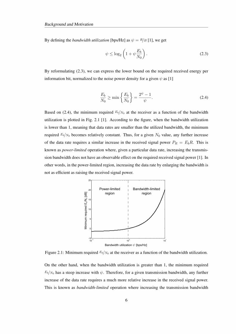
Based on (2.4), the minimum required Eb/N0 at the receiver as a function of the bandwidth
utilization is plotted in Fig. 2.1 [1]. According to the figure, when the bandwidth utilization
is lower than 1, meaning that data rates are smaller than the utilized bandwidth, the minimum
required Eb/N0 becomes relatively constant. Thus, for a given N0 value, any further increase
of the data rate requires a similar increase in the received signal power PR = EbR. This is
known as power-limited operation where, given a particular data rate, increasing the transmis-
sion bandwidth does not have an observable effect on the required received signal power [1]. In
other words, in the power-limited region, increasing the data rate by enlarging the bandwidth is
not as efficient as raising the received signal power.
10−1
100
101
−5
0
5
10
15
20
25
Bandwidth-limitedregion
Power-limitedregion
Bandwidthqutilizationqqqqq[bps/Hz]
Min
imum
qre
quire
dqE
b/N
0q[d
B]
Figure 2.1: Minimum required Eb/N0 at the receiver as a function of the bandwidth utilization.
On the other hand, when the bandwidth utilization is greater than 1, the minimum required
Eb/N0 has a steep increase with ψ. Therefore, for a given transmission bandwidth, any further
increase of the data rate requires a much more relative increase in the received signal power.
This is known as bandwidth-limited operation where increasing the transmission bandwidth
6
Background and Motivation
reduces the required received signal power for a certain data rate [1]. Putting it another way,
in the bandwidth-limited region, increasing the data rate by enlarging the bandwidth is a more
efficient way than raising the received signal power.
Above discussions assumed noise-limited scenarios where noise is the primary destructive
source. However, in real mobile communications, there is additional interference caused by
neighboring cells transmitting signal on the same frequency channel referred as inter-cell inter-
ference. In most cases, interference from neighboring cells has a more dominant effect on the
received signal than the noise itself also known as interference-limited scenario. The impact of
interference on a radio link is similar to that of noise. By taking the effect of interference into
account, the Shannon capacity given in (2.1) becomes
C = B × log2(1 +PRI + η
), (2.5)
where I is the total received interference power from neighboring cells and PR/I+η represents
the signal-to-interference-plus-noise power ratio (SINR). The principles discussed for power-
limited and bandwidth-limited regions also hold for the interference-limited scenarios.
As mentioned above, in power-limited regions, the most efficient way to increase the data rate
is to increase the received signal power. The simplest way of doing this is to increase the
transmission power, but this also increases the interference from neighboring cells with the
same ratio, hence brings no useful outcome. Thus, we should seek for solutions to enhance the
quality of the received signal without changing the transmission power.
Given a constant transmit power level, one way to increase the received signal power is reduc-
ing the cell size by deploying more transmitters with low power or by dividing the cell into
several sectors (cells) [12]. In the latter case, instead of using a single omnidirectional antenna,
several directional antennas are used. Thus, the same area is served by multiple antennas lead-
ing to multiple cells. With the reduced cell size, the distance between the transmitter and the
receiver is shortened. Therefore, the attenuation of the signal decreases and hence the received
signal power improves [13]. Reducing the cell size also increases the reuse of the resources
over the same geographical area, thus augments the resources allocated to the users. How-
ever, in interference-limited scenarios, decreasing the cell size also results in an increase in the
interference from neighboring cells.
Another method to improve the SINR is to increase the number of antennas at the receiver
7
Background and Motivation
and the transmitter sides. This technique is also known as multiple-input and multiple-output
(MIMO). Multiple antennas at the receiver can be used for achieving receive-antenna diversity
which improves the SINR of the received signal. Similarly, at the transmitter side multiple-
antennas can be used for transmit-antenna diversity. MIMO can also be used for focusing the
signal energy in one or more direction by using beamforming and precoding. Through this
way, both received signal power and data rates increase [14]. Using the MIMO technique for
achieving higher SINR values is an efficient solution as long as data rates are power limited. If
the bandwidth utilization is greater than 1, then any further increase in the number of antennas
corresponds to a marginal gain in the data rate. At this point, the convenient way is to use
MIMO for spatial multiplexing where multiple independent data signals are transmitted to a
single user at the same time [1]. The received signal power can also be increased by reducing
the noise at the receiver via use of more advanced receivers. For interference-limited scenarios,
techniques such as interference cancellation or interference alignment can be applied to enhance
the SINR at the receiver side.
QPSK 16QAM 64QAM
Figure 2.2: Signal constellations for QPSK, 16QAM and 64QAM.
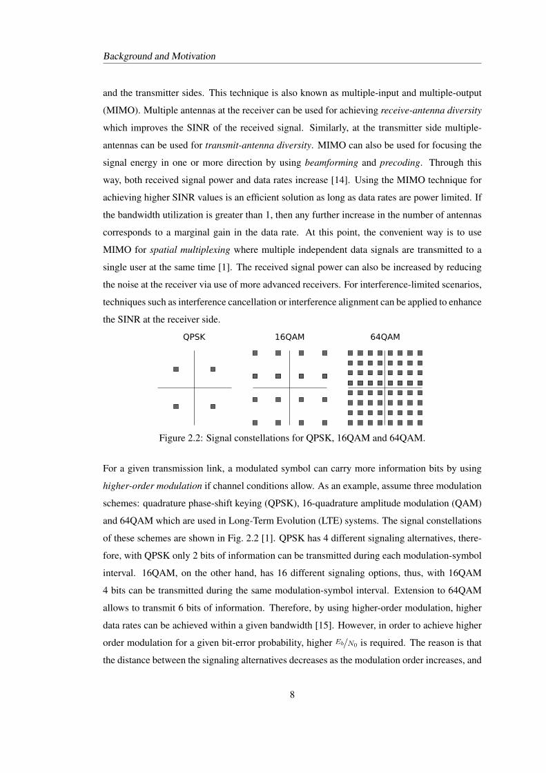
For a given transmission link, a modulated symbol can carry more information bits by using
higher-order modulation if channel conditions allow. As an example, assume three modulation
schemes: quadrature phase-shift keying (QPSK), 16-quadrature amplitude modulation (QAM)
and 64QAM which are used in Long-Term Evolution (LTE) systems. The signal constellations
of these schemes are shown in Fig. 2.2 [1]. QPSK has 4 different signaling alternatives, there-
fore, with QPSK only 2 bits of information can be transmitted during each modulation-symbol
interval. 16QAM, on the other hand, has 16 different signaling options, thus, with 16QAM
4 bits can be transmitted during the same modulation-symbol interval. Extension to 64QAM
allows to transmit 6 bits of information. Therefore, by using higher-order modulation, higher
data rates can be achieved within a given bandwidth [15]. However, in order to achieve higher
order modulation for a given bit-error probability, higher Eb/N0 is required. The reason is that
the distance between the signaling alternatives decreases as the modulation order increases, and
8
Background and Motivation
small distortion at the transmitted signal may cause a wrong decision at the receiver. Hence,
signals modulated with high-order schemes are less robust to interference and noise. This is
consistent with the plot given in Fig. 2.1 where given a limited bandwidth, higher bandwidth
utilization requires higher Eb/N0 at the receiver.
Time dispersion
frequency
Frequency selectivity
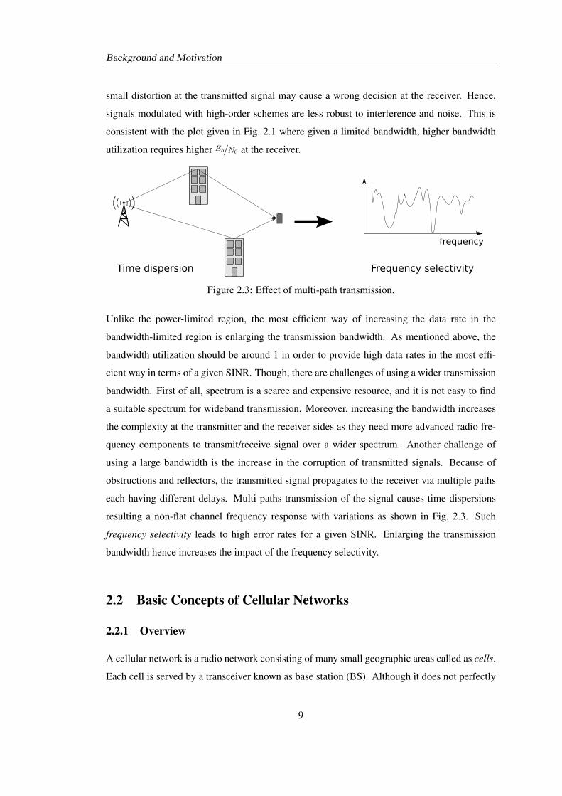
Figure 2.3: Effect of multi-path transmission.
Unlike the power-limited region, the most efficient way of increasing the data rate in the
bandwidth-limited region is enlarging the transmission bandwidth. As mentioned above, the
bandwidth utilization should be around 1 in order to provide high data rates in the most effi-
cient way in terms of a given SINR. Though, there are challenges of using a wider transmission
bandwidth. First of all, spectrum is a scarce and expensive resource, and it is not easy to find
a suitable spectrum for wideband transmission. Moreover, increasing the bandwidth increases
the complexity at the transmitter and the receiver sides as they need more advanced radio fre-
quency components to transmit/receive signal over a wider spectrum. Another challenge of
using a large bandwidth is the increase in the corruption of transmitted signals. Because of
obstructions and reflectors, the transmitted signal propagates to the receiver via multiple paths
each having different delays. Multi paths transmission of the signal causes time dispersions
resulting a non-flat channel frequency response with variations as shown in Fig. 2.3. Such
frequency selectivity leads to high error rates for a given SINR. Enlarging the transmission
bandwidth hence increases the impact of the frequency selectivity.
2.2 Basic Concepts of Cellular Networks
2.2.1 Overview
A cellular network is a radio network consisting of many small geographic areas called as cells.
Each cell is served by a transceiver known as base station (BS). Although it does not perfectly
9
Background and Motivation
match the case in reality, cells are mostly represented by hexagons.
A cell can serve multiple mobile transceivers with the wireless link between the BS and the
transceivers. In 3rd Generation Partnership Project (3GPP) [16], mobile transceivers are named
as user equipments (UEs). A UE can be any device such as a mobile phone that can connect to
the network. For simplicity, we use the term user instead of UE for the rest of the thesis.
BSs are connected to each other enabling users to communicate with other users even if they
are located in different cells. Also, cellular networks provide mobility of users via a handover
process that connects a user moving from one cell to another automatically to the other cell. As
a result, these connected cells provide a wide radio coverage area for users.
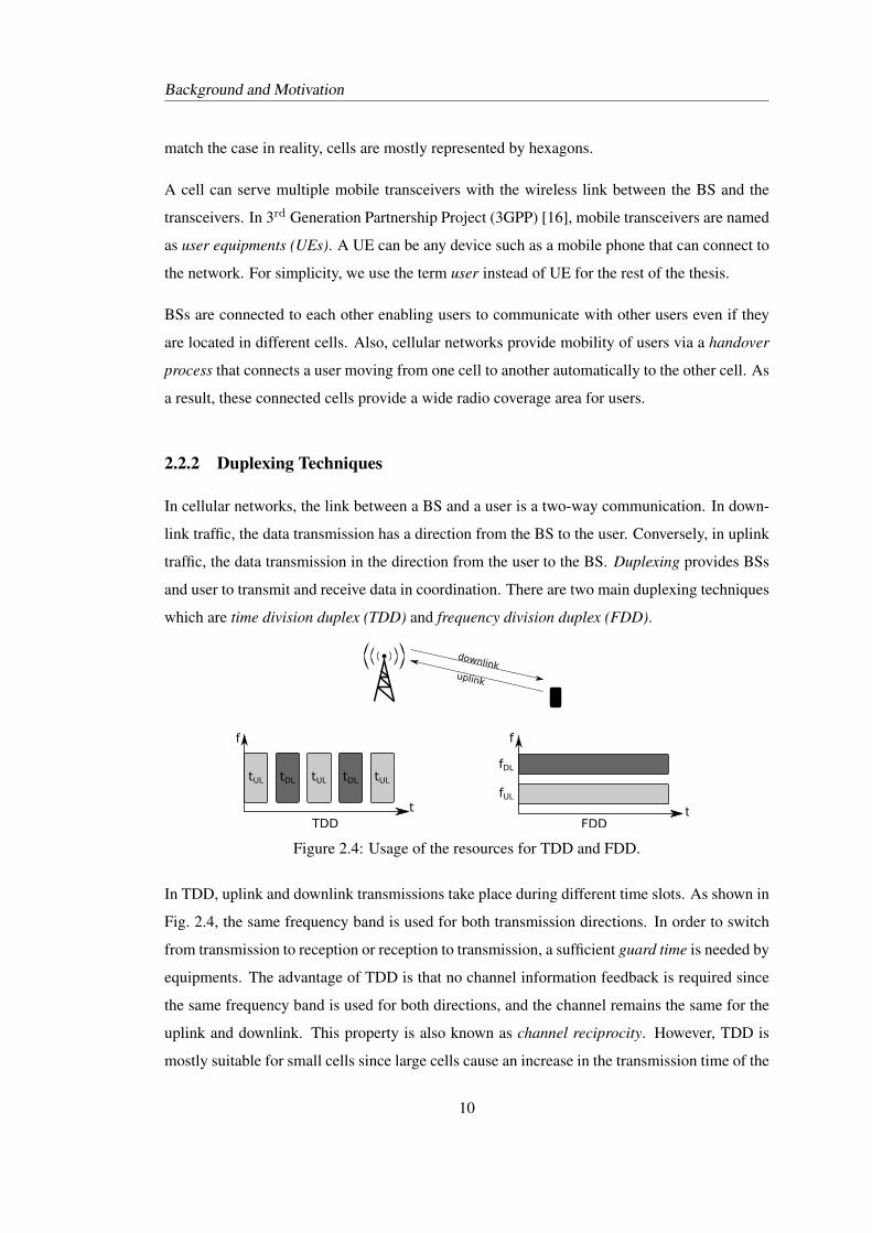
2.2.2 Duplexing Techniques
In cellular networks, the link between a BS and a user is a two-way communication. In down-
link traffic, the data transmission has a direction from the BS to the user. Conversely, in uplink
traffic, the data transmission in the direction from the user to the BS. Duplexing provides BSs
and user to transmit and receive data in coordination. There are two main duplexing techniques
which are time division duplex (TDD) and frequency division duplex (FDD).
t
f
fDL
fUL
FDDt
f
tUL tUL tULtDLtDL
TDD
downlinkuplink
Figure 2.4: Usage of the resources for TDD and FDD.
In TDD, uplink and downlink transmissions take place during different time slots. As shown in
Fig. 2.4, the same frequency band is used for both transmission directions. In order to switch
from transmission to reception or reception to transmission, a sufficient guard time is needed by
equipments. The advantage of TDD is that no channel information feedback is required since
the same frequency band is used for both directions, and the channel remains the same for the
uplink and downlink. This property is also known as channel reciprocity. However, TDD is
mostly suitable for small cells since large cells cause an increase in the transmission time of the
10
Background and Motivation
signals, i.e. tDL and tUL in Fig. 2.4. Thus, in a given time period, a small amount of data can
be transmitted in a large cell so making the system inefficient [12].
In FDD, uplink and downlink transmissions take place in separated frequency bands with a suf-
ficient duplex separation in the frequency domain. Therefore, FDD requires a paired spectrum,
whereas, TDD can be applied in an unpaired spectrum. Fig. 2.4 implies that, with FDD, uplink
and downlink transmissions occur simultaneously also known as full-duplex operation.
As a final remark, some user cannot transmit and receive signals simultaneously. For such user,
half-duplex FDD is used in LTE where the users receive and transmit at different frequency
bands during different time slots [1].
2.2.3 Multiple Access Methods
Sharing of resources by users within a cell in a coordinated way is known as multiple access.
The most basic multiple access methods used in wireless networks are time division multiple
access (TDMA) and frequency division multiple access (FDMA). In addition to TDMA and
FDMA, other well-known access techniques are code division multiple access (CDMA), which
is mainly used in 3rd Generation (3G) networks, and orthogonal frequency division multiple
access (OFDMA) that is considered in future wireless networks such as LTE and Worldwide
Interoperability for Microwave Access (WiMAX).
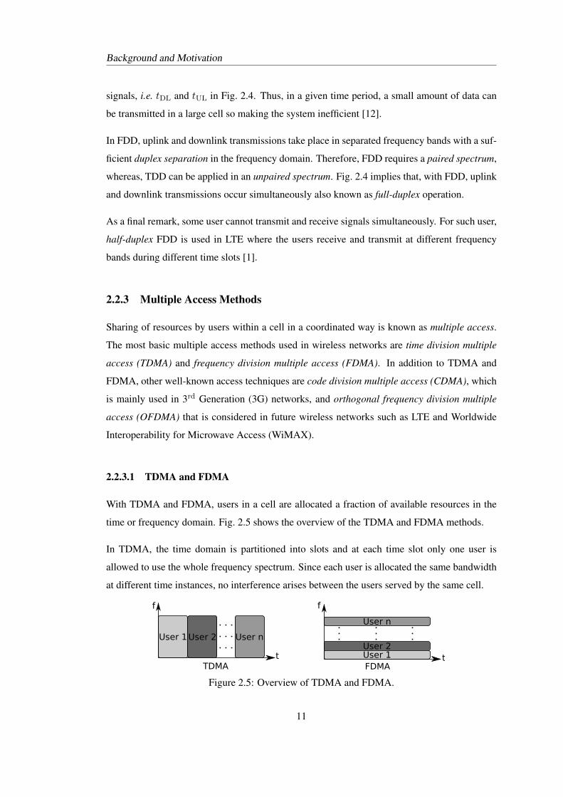
2.2.3.1 TDMA and FDMA
With TDMA and FDMA, users in a cell are allocated a fraction of available resources in the
time or frequency domain. Fig. 2.5 shows the overview of the TDMA and FDMA methods.
In TDMA, the time domain is partitioned into slots and at each time slot only one user is
allowed to use the whole frequency spectrum. Since each user is allocated the same bandwidth
at different time instances, no interference arises between the users served by the same cell.
t
f
User 1
TDMA
User 2 User n
t
f
FDMA
User n
User 1User 2
Figure 2.5: Overview of TDMA and FDMA.
11
Background and Motivation
In FDMA, on the other hand, the frequency spectrum is partitioned into well-separated channels
such that they do not interfere with each other. Each channel is allocated to only one user during
the operation time. Since users are allocated to non-overlapping channels, users at the same cell
do not face interference from each other.
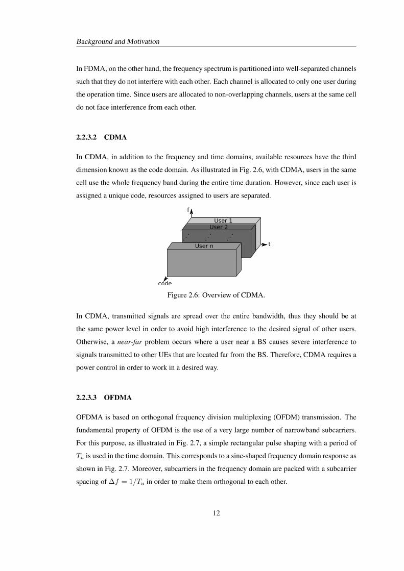
2.2.3.2 CDMA
In CDMA, in addition to the frequency and time domains, available resources have the third
dimension known as the code domain. As illustrated in Fig. 2.6, with CDMA, users in the same
cell use the whole frequency band during the entire time duration. However, since each user is
assigned a unique code, resources assigned to users are separated.
t
f
User 1 User 2
User n
code
Figure 2.6: Overview of CDMA.
In CDMA, transmitted signals are spread over the entire bandwidth, thus they should be at
the same power level in order to avoid high interference to the desired signal of other users.
Otherwise, a near-far problem occurs where a user near a BS causes severe interference to
signals transmitted to other UEs that are located far from the BS. Therefore, CDMA requires a
power control in order to work in a desired way.
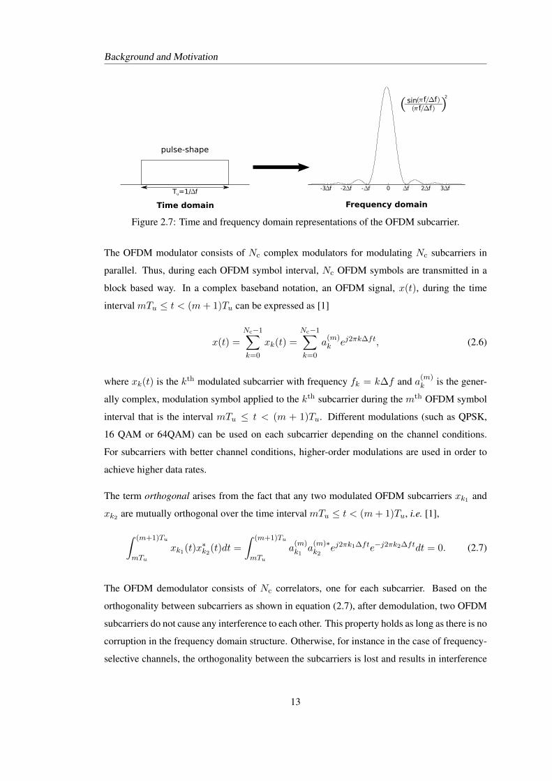
2.2.3.3 OFDMA
OFDMA is based on orthogonal frequency division multiplexing (OFDM) transmission. The
fundamental property of OFDM is the use of a very large number of narrowband subcarriers.
For this purpose, as illustrated in Fig. 2.7, a simple rectangular pulse shaping with a period of
Tu is used in the time domain. This corresponds to a sinc-shaped frequency domain response as
shown in Fig. 2.7. Moreover, subcarriers in the frequency domain are packed with a subcarrier
spacing of ∆f = 1/Tu in order to make them orthogonal to each other.
12
Background and Motivation
f2 f3f-f-2f-3 f0
ffsinff
2
fTu=1/
pulse-shape
Time domain Frequency domain
Figure 2.7: Time and frequency domain representations of the OFDM subcarrier.
The OFDM modulator consists of Nc complex modulators for modulating Nc subcarriers in
parallel. Thus, during each OFDM symbol interval, Nc OFDM symbols are transmitted in a
block based way. In a complex baseband notation, an OFDM signal, x(t), during the time
interval mTu ≤ t < (m+ 1)Tu can be expressed as [1]
x(t) =
Nc−1∑k=0
xk(t) =
Nc−1∑k=0
a(m)k ej2πk∆ft, (2.6)
where xk(t) is the kth modulated subcarrier with frequency fk = k∆f and a(m)k is the gener-
ally complex, modulation symbol applied to the kth subcarrier during the mth OFDM symbol
interval that is the interval mTu ≤ t < (m + 1)Tu. Different modulations (such as QPSK,
16 QAM or 64QAM) can be used on each subcarrier depending on the channel conditions.
For subcarriers with better channel conditions, higher-order modulations are used in order to
achieve higher data rates.
The term orthogonal arises from the fact that any two modulated OFDM subcarriers xk1 and
xk2 are mutually orthogonal over the time interval mTu ≤ t < (m+ 1)Tu, i.e. [1],
∫ (m+1)Tu
mTu
xk1(t)x∗k2(t)dt =
∫ (m+1)Tu
mTu
a(m)k1
a(m)∗k2
ej2πk1∆fte−j2πk2∆ftdt = 0. (2.7)
The OFDM demodulator consists of Nc correlators, one for each subcarrier. Based on the
orthogonality between subcarriers as shown in equation (2.7), after demodulation, two OFDM
subcarriers do not cause any interference to each other. This property holds as long as there is no
corruption in the frequency domain structure. Otherwise, for instance in the case of frequency-
selective channels, the orthogonality between the subcarriers is lost and results in interference
13
Background and Motivation
between subcarriers. This problem is also known as inter-symbol interference. Therefore, in
order to make the OFDM signal robust to frequency-selective radio channels, a cyclic-prefix
is inserted between OFDM symbols in the time domain [1]. Since the cyclic prefix increases
the system overhead, it decreases the resource utilization of the system. Another condition for
proper demodulation of the subcarriers is that the transmitter and the receiver should operate
at the same reference frequency. Any mismatch between them causes the loss of orthogonality
between the subcarriers.
Freq
uenc
y (s
ubca
rrie
r num
ber)
Time (OFDM symbol number)
m-2 m-1 m m+1 m+2
01
k
Nc-2Nc-1
Figure 2.8: Overview of an OFDM transmission in the time and frequency domains.
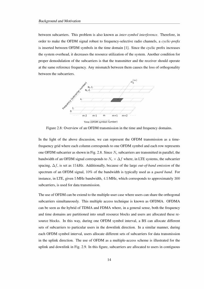
In the light of the above discussion, we can represent the OFDM transmission as a time-
frequency grid where each column corresponds to one OFDM symbol and each row represents
one OFDM subcarrier as shown in Fig. 2.8. SinceNc subcarriers are transmitted in parallel, the
bandwidth of an OFDM signal corresponds to Nc ×∆f where, in LTE systems, the subcarrier
spacing, ∆f , is set as 15 kHz. Additionally, because of the large out-of-band emission of the
spectrum of an OFDM signal, 10% of the bandwidth is typically used as a guard band. For
instance, in LTE, given 5 MHz bandwidth, 4.5 MHz, which corresponds to approximately 300
subcarriers, is used for data transmission.
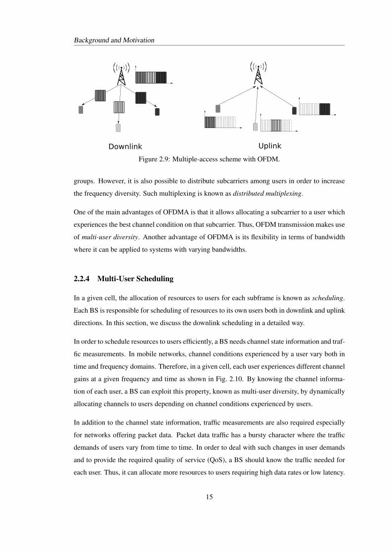
The use of OFDM can be extend to the multiple-user case where users can share the orthogonal
subcarriers simultaneously. This multiple access technique is known as OFDMA. OFDMA
can be seen as the hybrid of TDMA and FDMA where, in a general sense, both the frequency
and time domains are partitioned into small resource blocks and users are allocated these re-
source blocks. In this way, during one OFDM symbol interval, a BS can allocate different
sets of subcarriers to particular users in the downlink direction. In a similar manner, during
each OFDM symbol interval, users allocate different sets of subcarriers for data transmission
in the uplink direction. The use of OFDM as a multiple-access scheme is illustrated for the
uplink and downlink in Fig. 2.9. In this figure, subcarriers are allocated to users in contiguous
14
Background and Motivation
Downlink Uplink
Figure 2.9: Multiple-access scheme with OFDM.
groups. However, it is also possible to distribute subcarriers among users in order to increase
the frequency diversity. Such multiplexing is known as distributed multiplexing.
One of the main advantages of OFDMA is that it allows allocating a subcarrier to a user which
experiences the best channel condition on that subcarrier. Thus, OFDM transmission makes use
of multi-user diversity. Another advantage of OFDMA is its flexibility in terms of bandwidth
where it can be applied to systems with varying bandwidths.
2.2.4 Multi-User Scheduling
In a given cell, the allocation of resources to users for each subframe is known as scheduling.
Each BS is responsible for scheduling of resources to its own users both in downlink and uplink
directions. In this section, we discuss the downlink scheduling in a detailed way.
In order to schedule resources to users efficiently, a BS needs channel state information and traf-
fic measurements. In mobile networks, channel conditions experienced by a user vary both in
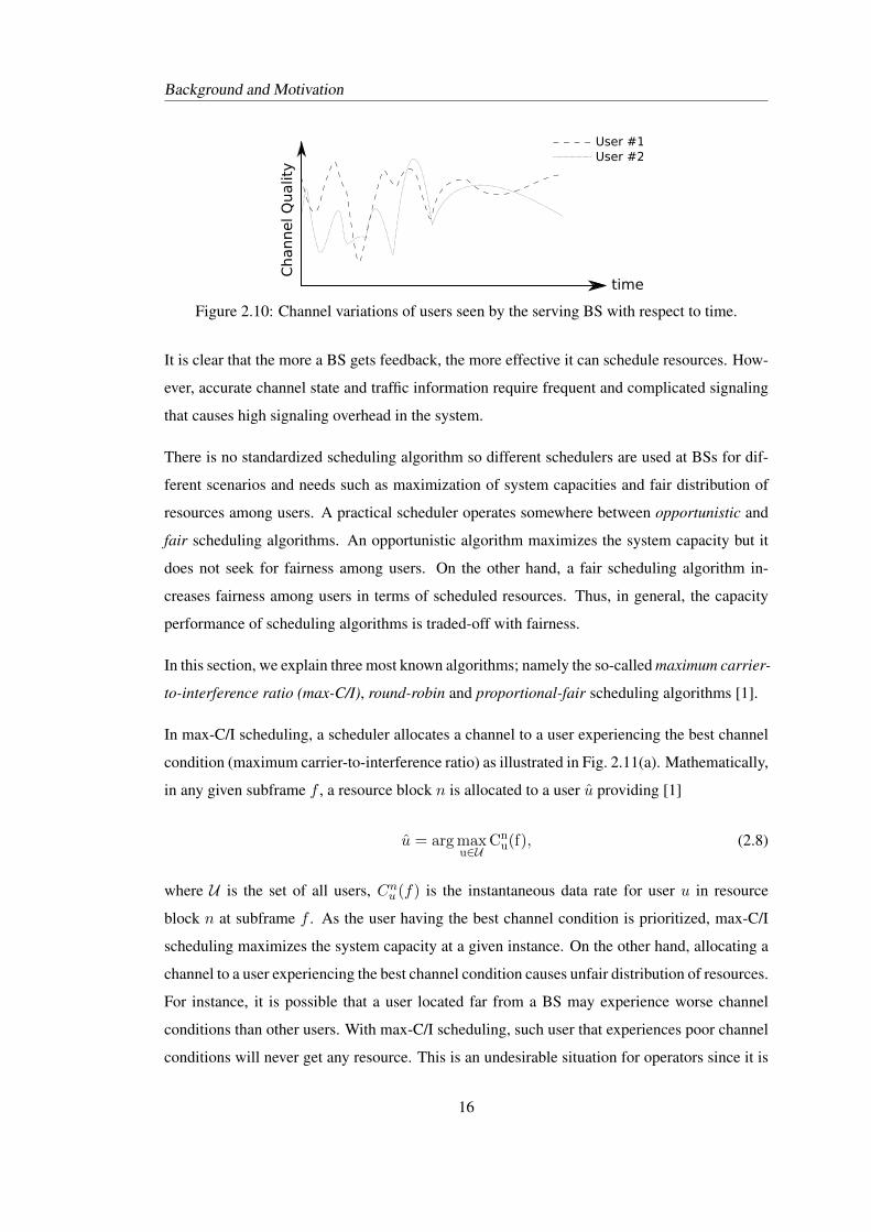
time and frequency domains. Therefore, in a given cell, each user experiences different channel
gains at a given frequency and time as shown in Fig. 2.10. By knowing the channel informa-
tion of each user, a BS can exploit this property, known as multi-user diversity, by dynamically
allocating channels to users depending on channel conditions experienced by users.
In addition to the channel state information, traffic measurements are also required especially
for networks offering packet data. Packet data traffic has a bursty character where the traffic
demands of users vary from time to time. In order to deal with such changes in user demands
and to provide the required quality of service (QoS), a BS should know the traffic needed for
each user. Thus, it can allocate more resources to users requiring high data rates or low latency.
15
Background and Motivation
timeC
hannel Q
ualit
y
User #1User #2
Figure 2.10: Channel variations of users seen by the serving BS with respect to time.
It is clear that the more a BS gets feedback, the more effective it can schedule resources. How-
ever, accurate channel state and traffic information require frequent and complicated signaling
that causes high signaling overhead in the system.
There is no standardized scheduling algorithm so different schedulers are used at BSs for dif-
ferent scenarios and needs such as maximization of system capacities and fair distribution of
resources among users. A practical scheduler operates somewhere between opportunistic and
fair scheduling algorithms. An opportunistic algorithm maximizes the system capacity but it
does not seek for fairness among users. On the other hand, a fair scheduling algorithm in-
creases fairness among users in terms of scheduled resources. Thus, in general, the capacity
performance of scheduling algorithms is traded-off with fairness.
In this section, we explain three most known algorithms; namely the so-called maximum carrier-
to-interference ratio (max-C/I), round-robin and proportional-fair scheduling algorithms [1].
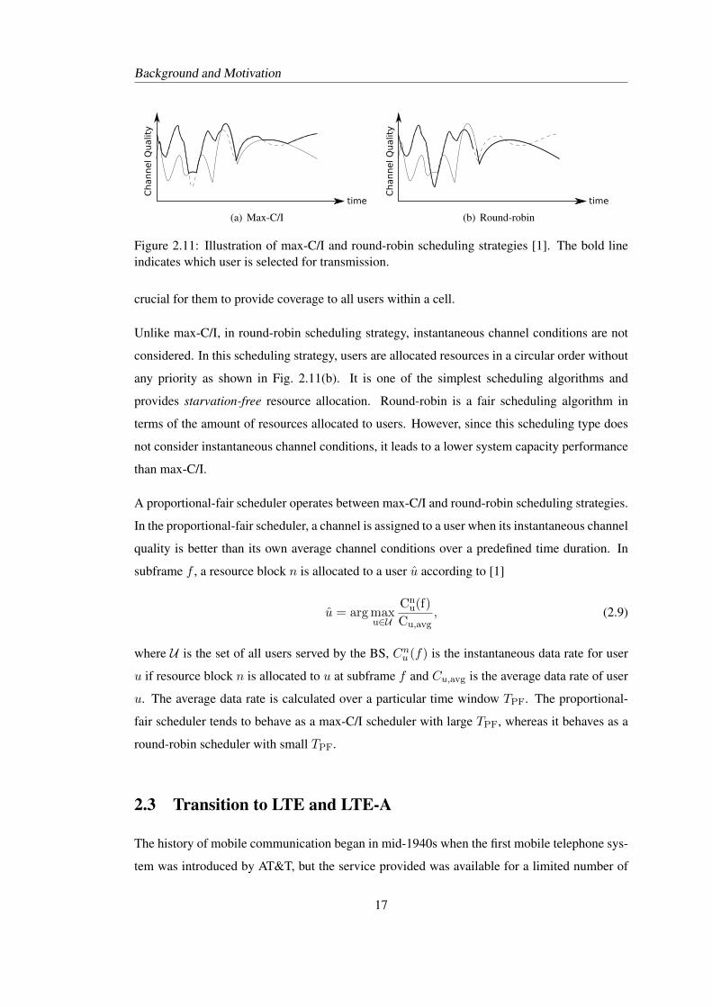
In max-C/I scheduling, a scheduler allocates a channel to a user experiencing the best channel
condition (maximum carrier-to-interference ratio) as illustrated in Fig. 2.11(a). Mathematically,
in any given subframe f , a resource block n is allocated to a user u providing [1]
u = arg maxu∈U
Cnu(f), (2.8)
where U is the set of all users, Cnu (f) is the instantaneous data rate for user u in resource
block n at subframe f . As the user having the best channel condition is prioritized, max-C/I
scheduling maximizes the system capacity at a given instance. On the other hand, allocating a
channel to a user experiencing the best channel condition causes unfair distribution of resources.
For instance, it is possible that a user located far from a BS may experience worse channel
conditions than other users. With max-C/I scheduling, such user that experiences poor channel
conditions will never get any resource. This is an undesirable situation for operators since it is
16
Background and Motivation
time
Ch
an
nel Q
ualit
y
(a) Max-C/I
time
Ch
an
nel Q
ualit
y
(b) Round-robin
Figure 2.11: Illustration of max-C/I and round-robin scheduling strategies [1]. The bold lineindicates which user is selected for transmission.
crucial for them to provide coverage to all users within a cell.
Unlike max-C/I, in round-robin scheduling strategy, instantaneous channel conditions are not
considered. In this scheduling strategy, users are allocated resources in a circular order without
any priority as shown in Fig. 2.11(b). It is one of the simplest scheduling algorithms and
provides starvation-free resource allocation. Round-robin is a fair scheduling algorithm in
terms of the amount of resources allocated to users. However, since this scheduling type does
not consider instantaneous channel conditions, it leads to a lower system capacity performance
than max-C/I.
A proportional-fair scheduler operates between max-C/I and round-robin scheduling strategies.
In the proportional-fair scheduler, a channel is assigned to a user when its instantaneous channel
quality is better than its own average channel conditions over a predefined time duration. In
subframe f , a resource block n is allocated to a user u according to [1]
u = arg maxu∈U
Cnu(f)
Cu,avg, (2.9)
where U is the set of all users served by the BS, Cnu (f) is the instantaneous data rate for user
u if resource block n is allocated to u at subframe f and Cu,avg is the average data rate of user
u. The average data rate is calculated over a particular time window TPF. The proportional-
fair scheduler tends to behave as a max-C/I scheduler with large TPF, whereas it behaves as a
round-robin scheduler with small TPF.
2.3 Transition to LTE and LTE-A
The history of mobile communication began in mid-1940s when the first mobile telephone sys-
tem was introduced by AT&T, but the service provided was available for a limited number of
17
Background and Motivation
users. In 1980s, the first well-known international mobile communication systems, called 1st
Generation (1G) cellular systems, were developed. The most famous ones were the Nordic
Mobile Telephony (NMT) system introduced in Nordic Countries, Advanced Mobile Phone
Service (AMPS) in USA and Australia, Total Access Communications System (TACS) in UK
and Japanese Total Access Communications System (J-TACS) in Japan. The 1G was an analog
cellular system and supported plain old telephone service (voice with some related supplemen-
tary services). Additionally, with 1G, the concept of roaming was developed, thus users moving
outside the area of their home operator could get service from other operators. However, the
voice quality in 1G networks was not consistent and sometimes cross-talk happened between
users.
The evolution to ‘digital’ 2nd Generation (2G) networks started during 1980s. In Europe, the
Conference Europeenne des Administrations des Postes et des Telecommunications (CEPT)
created the Global System for Mobile Communications (GSM) to develop a pan-European
standard for a mobile telephone system. Later, the responsibility of the GSM development
was taken by European Telecommunications Standards Institute (ETSI). In the beginning of
1990s, the first GSM network was deployed by Radiolinja in Finland. In GSM, the spectrum
is divided into multiple channels of 200 kHz and each channel is shared by maximum 8 users
using TDMA. Although GSM was a pan-European project, it gained worldwide interest and
deployed by other countries all over the world. Another feature of the GSM is the use of a sub-
scriber identity module (SIM) card which carriers the owner’s identity information. Therefore,
a GSM phone does not work without a SIM card. In addition to GSM, in 1993, IS-95 based on
CDMA was introduced in USA. CDMA uses channels with 1.25 MHz wide and it can support
up to 64 users with orthogonal codes.
Compared to 1G, 2G networks offer higher system capacity and better service quality. In
addition to voice service, 2G networks could also offer data services such as short message
service (SMS) and circuit-switched data services like sending and receiving e-mails. During
the second half of the 1990s, General Packet Radio Services (GPRS), which are often named
as 2.5G, were introduced. The importance of the GPRS was being the first packet data service.
The further improvement of data rate was achieved with the introduction of enhanced data rates
for global evolution (EDGE).
The research on 3G networks, also known as International Mobile Telecommunications-2000
(IMT-2000) [17], began in 1980s by International Telecommunication Union (ITU). During
18
Background and Motivation
1990s, the 3G research activities gained more momentum in parallel to widespread deployment
of 2G networks. Also, in 1998, an international consortium named 3GPP [16] was formed
by several international standardization organizations from Europe, USA, Japan, China and
Korea. The aim of 3GPP is to develop aligned specifications worldwide instead of parallel
development. In early 2000s, the first 3G networks based on CDMA were deployed.
The widespread of 2G and 3G systems eventually causes a rapid growing of the number of
users. Additionally, user requirements are evolving with new handsets offering multimedia
applications and packet data services. For instance, in 2016, video services are expected to
constitute the 70 % of the wireless traffic [18]. Such challenges were the main driver for evo-
lution to 3GPP LTE systems. 3GPP started to work on LTE in 2004, and the requirements and
design targets for LTE were finalized in so-called 3GPP Release-8 in 2005 [4]. After Release-
8, in Release-9, further enhancements for LTE are defined. A summary of LTE specifications
described in Release-8 and 9 are listed as following [1]:
• One of the significant changes in LTE is that it supports packet-switched services instead
of circuit-switched services as used in previous generations.
• LTE promises to satisfy the relentless demand for data rates by offering a peak data rate
of 300 Mbps for downlink and 75 Mbps for uplink transmissions.
• In the standard LTE air interface, OFDM is the driving technology. The major advantage
of OFDM is its robustness against frequency selectivity.
• Due to the building-block like structure of the OFDM time-frequency grid, LTE intro-
duces a high degree of flexibility in network operation and supports multiple choice of
bandwidths ranging from 1.4 to 20 MHz.
• OFDM supports channel-dependent scheduling both in time and frequency domains, giv-
ing a scheduler more flexibility to allocate the most appropriate resources to users ac-
cording to the channel conditions. Additionally, the scheduler in LTE can adapt the data
rates to be used for each user depending on the channel conditions and traffic load of the
network.
• LTE provides low latency communications via an improved network architecture.
• LTE supports multi-antenna transmission that allows high data rates and improved inter-
ference handling.
19
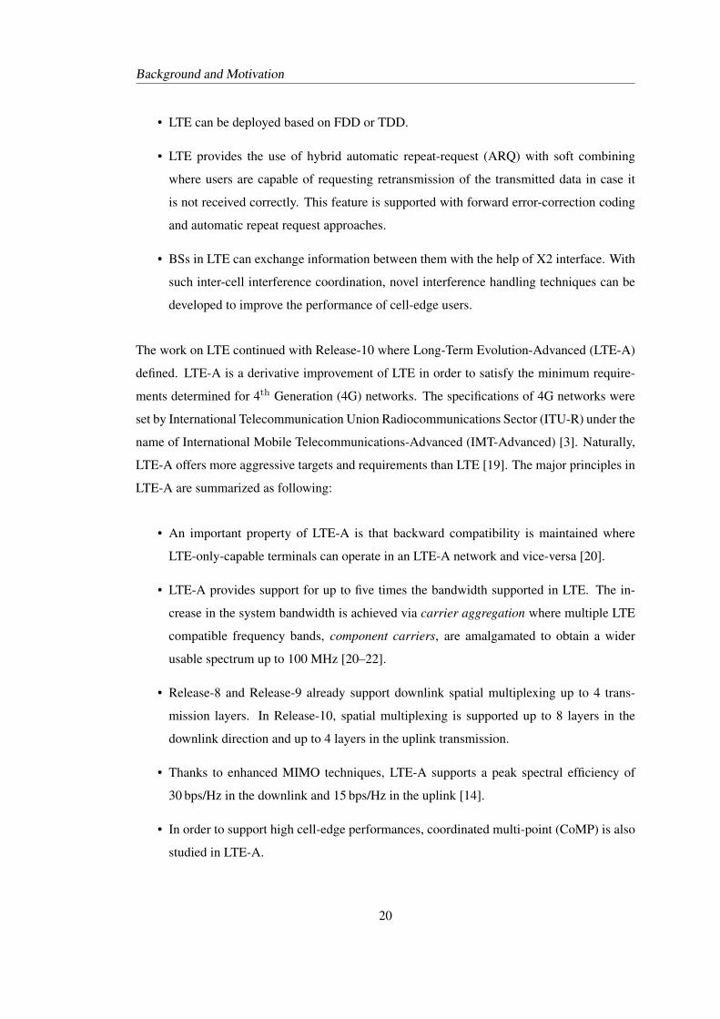
Background and Motivation
• LTE can be deployed based on FDD or TDD.
• LTE provides the use of hybrid automatic repeat-request (ARQ) with soft combining
where users are capable of requesting retransmission of the transmitted data in case it
is not received correctly. This feature is supported with forward error-correction coding
and automatic repeat request approaches.
• BSs in LTE can exchange information between them with the help of X2 interface. With
such inter-cell interference coordination, novel interference handling techniques can be
developed to improve the performance of cell-edge users.
The work on LTE continued with Release-10 where Long-Term Evolution-Advanced (LTE-A)
defined. LTE-A is a derivative improvement of LTE in order to satisfy the minimum require-
ments determined for 4th Generation (4G) networks. The specifications of 4G networks were
set by International Telecommunication Union Radiocommunications Sector (ITU-R) under the
name of International Mobile Telecommunications-Advanced (IMT-Advanced) [3]. Naturally,
LTE-A offers more aggressive targets and requirements than LTE [19]. The major principles in
LTE-A are summarized as following:
• An important property of LTE-A is that backward compatibility is maintained where
LTE-only-capable terminals can operate in an LTE-A network and vice-versa [20].
• LTE-A provides support for up to five times the bandwidth supported in LTE. The in-
crease in the system bandwidth is achieved via carrier aggregation where multiple LTE
compatible frequency bands, component carriers, are amalgamated to obtain a wider
usable spectrum up to 100 MHz [20–22].
• Release-8 and Release-9 already support downlink spatial multiplexing up to 4 trans-
mission layers. In Release-10, spatial multiplexing is supported up to 8 layers in the
downlink direction and up to 4 layers in the uplink transmission.
• Thanks to enhanced MIMO techniques, LTE-A supports a peak spectral efficiency of
30 bps/Hz in the downlink and 15 bps/Hz in the uplink [14].
• In order to support high cell-edge performances, coordinated multi-point (CoMP) is also
studied in LTE-A.
20
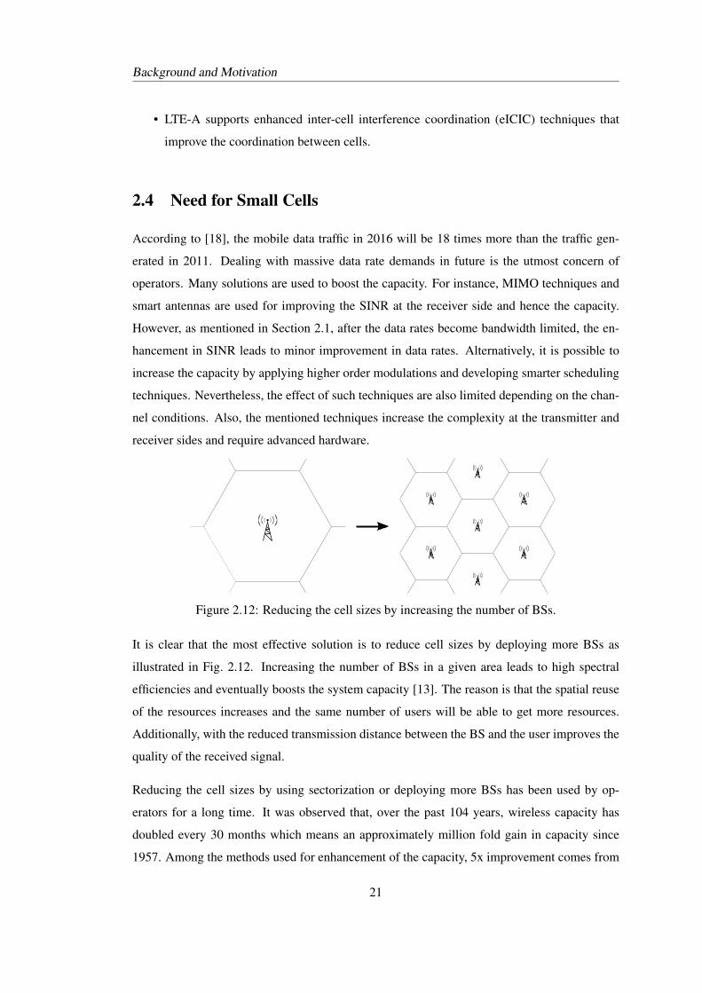
Background and Motivation
• LTE-A supports enhanced inter-cell interference coordination (eICIC) techniques that
improve the coordination between cells.
2.4 Need for Small Cells
According to [18], the mobile data traffic in 2016 will be 18 times more than the traffic gen-
erated in 2011. Dealing with massive data rate demands in future is the utmost concern of
operators. Many solutions are used to boost the capacity. For instance, MIMO techniques and
smart antennas are used for improving the SINR at the receiver side and hence the capacity.
However, as mentioned in Section 2.1, after the data rates become bandwidth limited, the en-
hancement in SINR leads to minor improvement in data rates. Alternatively, it is possible to
increase the capacity by applying higher order modulations and developing smarter scheduling
techniques. Nevertheless, the effect of such techniques are also limited depending on the chan-
nel conditions. Also, the mentioned techniques increase the complexity at the transmitter and
receiver sides and require advanced hardware.
Figure 2.12: Reducing the cell sizes by increasing the number of BSs.
It is clear that the most effective solution is to reduce cell sizes by deploying more BSs as
illustrated in Fig. 2.12. Increasing the number of BSs in a given area leads to high spectral
efficiencies and eventually boosts the system capacity [13]. The reason is that the spatial reuse
of the resources increases and the same number of users will be able to get more resources.
Additionally, with the reduced transmission distance between the BS and the user improves the
quality of the received signal.
Reducing the cell sizes by using sectorization or deploying more BSs has been used by op-
erators for a long time. It was observed that, over the past 104 years, wireless capacity has
doubled every 30 months which means an approximately million fold gain in capacity since
1957. Among the methods used for enhancement of the capacity, 5x improvement comes from
21
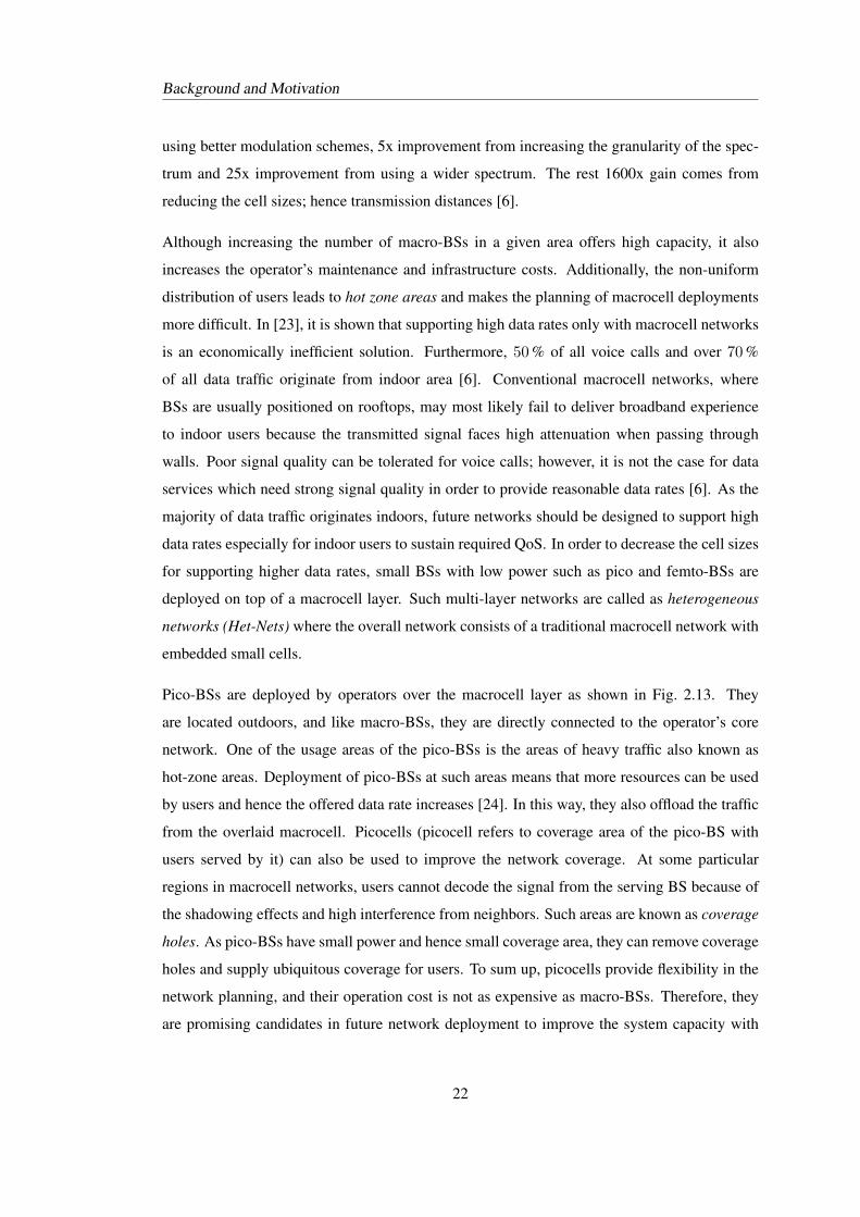
Background and Motivation
using better modulation schemes, 5x improvement from increasing the granularity of the spec-
trum and 25x improvement from using a wider spectrum. The rest 1600x gain comes from
reducing the cell sizes; hence transmission distances [6].
Although increasing the number of macro-BSs in a given area offers high capacity, it also
increases the operator’s maintenance and infrastructure costs. Additionally, the non-uniform
distribution of users leads to hot zone areas and makes the planning of macrocell deployments
more difficult. In [23], it is shown that supporting high data rates only with macrocell networks
is an economically inefficient solution. Furthermore, 50 % of all voice calls and over 70 %
of all data traffic originate from indoor area [6]. Conventional macrocell networks, where
BSs are usually positioned on rooftops, may most likely fail to deliver broadband experience
to indoor users because the transmitted signal faces high attenuation when passing through
walls. Poor signal quality can be tolerated for voice calls; however, it is not the case for data
services which need strong signal quality in order to provide reasonable data rates [6]. As the
majority of data traffic originates indoors, future networks should be designed to support high
data rates especially for indoor users to sustain required QoS. In order to decrease the cell sizes
for supporting higher data rates, small BSs with low power such as pico and femto-BSs are
deployed on top of a macrocell layer. Such multi-layer networks are called as heterogeneous
networks (Het-Nets) where the overall network consists of a traditional macrocell network with
embedded small cells.
Pico-BSs are deployed by operators over the macrocell layer as shown in Fig. 2.13. They
are located outdoors, and like macro-BSs, they are directly connected to the operator’s core
network. One of the usage areas of the pico-BSs is the areas of heavy traffic also known as
hot-zone areas. Deployment of pico-BSs at such areas means that more resources can be used
by users and hence the offered data rate increases [24]. In this way, they also offload the traffic
from the overlaid macrocell. Picocells (picocell refers to coverage area of the pico-BS with
users served by it) can also be used to improve the network coverage. At some particular
regions in macrocell networks, users cannot decode the signal from the serving BS because of
the shadowing effects and high interference from neighbors. Such areas are known as coverage
holes. As pico-BSs have small power and hence small coverage area, they can remove coverage
holes and supply ubiquitous coverage for users. To sum up, picocells provide flexibility in the
network planning, and their operation cost is not as expensive as macro-BSs. Therefore, they
are promising candidates in future network deployment to improve the system capacity with
22
Background and Motivation
pico-BS
pico-BS
pico-BSpico-BS
pico-BS
Figure 2.13: A multi-layer network deployment with macro and pico-BSs.
low cost burden to the operators.
In contrast to pico-BSs, femto-BSs, or home evolved NodeB (HeNB) according to 3GPP ter-
minology, are mainly deployed indoors to improve the coverage and data rates for indoor users.
These BSs are inexpensive and short-range devices, and more importantly they can be deployed
by end users in an ad hoc fashion such as Wireless Fidelity (Wi-Fi) access points. Therefore,
femtocells (femtocell refers to coverage area of the femto-BS with users served by it) have a
dynamic environment where the number and location of femto-BSs can change during the op-
eration of the network as they are turned on or off. Such network deployments are also called
uncoordinated networks since, unlike macro and pico-BSs, operator cannot determine the loca-
tions of the neighboring BSs a priori. Moreover, as these BSs are deployed indoor places like
private homes, the connection between the femto-BS and the operator’s core network can be
achieved via the existing broadband connections such as digital subscriber line (DSL) [25, 26].
Another novelty coming with femtocells is that they offer different access policies depending
on their usage purpose. Thus, femto-BSs can serve either all users without any restriction or
only a group of subscribed users depending on the deployment strategy.
2.5 Interference Mitigation at Small Cell Networks
The major drawback of Het-Nets is the increase in co-channel interference. Interference mit-
igation is crucial especially for cell-edge users which are located near the boundary of two or
more cells and face high interference. Therefore, these users get service with low data rates, or
in some cases, they cannot decode the data transmitted from the serving BS and they go into
outage.
23
Background and Motivation
In order to mitigate interference in picocell networks, the traditional network planning and
optimization techniques used for macrocells can be applied to these networks up to some extent.
Similar to macrocell networks, an operator has full control over the picocell network so it can
decide the locations of pico-BSs to be deployed, and activate or deactivate pico-BSs depending
on the environment. Moreover, access to pico-BSs is open to all users where users can easily
hand over to a pico-BS if they experience a high received power level. Such properties of the
picocell network make the interference predictable to some extent, hence allow efficient use of
conventional static interference mitigation techniques used for macrocell networks.
Unlike picocell and macrocell networks, interference mitigation becomes more challenging in
femtocell networks particularly when BSs are densely and randomly deployed without sophis-
ticated planning of the network topology. Also, as femto-BSs are deployed by end users in
order to get better QoS, the expectation of these users becomes higher than the macro-users.
Thus, interference mitigation becomes more crucial for such networks.
The uncoordinated deployment of femto-BSs indicates the necessity for dynamic interference
mitigation techniques that automatically adapt to the observed interference conditions. At such
networks, since the operator does not have full control over the network, the traditional network
planning cannot be adequately applied. Also, a femto-BS, which serves only a set of subscribed
users, causes high interference to unsubscribed users located nearby. Another challenge of the
femto-BSs is that they are planned to be bought by end users so they should be affordable in
terms of price. Therefore, their hardware cannot be as advanced as macro-BSs. Furthermore,
the broadband technology used for backhauling has more latency than the backhaul provided
for macrocell networks. With such limitations, complex interference mitigation techniques
requiring low backhaul latency and advanced antenna systems cannot be applied to femtocell
networks.
To sum up, the mentioned challenges of femtocell networks indicate the necessity of new ap-
proaches to deal with interference in such networks. It is clear that the conventional methods
are not capable of solving the interference problem in femtocell networks. The interference
mitigation should be more dynamic and should respond to changes in a network efficiently in
a short time. This additionally brings the requirement of methods with low complexity in term
of hardware and signaling.
To develop interference mitigation techniques for femtocell networks is the primary motivation
24
Background and Motivation
of this thesis. The aim is to reduce downlink interference to improve the performance of the
cell-edge users without causing a sharp decrease in the network capacity. We give our attention
mainly to interference between femtocells and follow the interference avoidance methods by
using resource partitioning techniques. Because of the unpredictable and dynamic interference
environment, we focus on an interference mitigation technique which is dynamic in a sense that
it can update itself depending on the changes in the environment. As a system model, we use
approaches in line with the LTE and LTE-A specifications and develop methods to be easily
applied to these systems without increasing the complexity at the user and BS side.
25

Background and Motivation
26
Chapter 3Femtocell Networks: An Overview
3.1 Introduction
Femto-base stations (BSs) are planned to be deployed primarily for indoor places to provide
high indoor data rates and service quality. Being a cheap and easy solution, femto-BSs have
become one of the promising network elements for improving the indoor coverage and offload-
ing the macrocell traffic. 60% of the operators believe that, in future network deployments,
small cells will have a more significant role than macrocells, and indeed as of 2013, customer
femto-BSs have already outnumbered macro-BSs [10]. The growing importance of femtocells
has accelerated the standardization efforts on femtocells. The primary standardization orga-
nization for femtocells is 3rd Generation Partnership Project (3GPP) [16]. Apart from 3GPP,
Small Cell Forum (formerly Femto Forum), a non-profit organization, founded in 2007 with
several vendors and operators, has also contributed to the standardization process [27]. The
European Union also funded a project called ‘Broadband Evolved FEMTO Networks’ in order
to develop future femtocell technologies for improved and broader femtocell services [28].
Unlike macro-BSs, femto-BSs are small scale BSs with low power and low cost and by their
very nature they can be deployed randomly by end users. These unique properties of femtocell
networks differentiate them from macrocell networks in many aspects including access poli-
cies and the number of served users. As this thesis mainly focuses on femtocell networks, it
is crucial to understand femtocell networks and their corresponding challenges in order to de-
velop effective interference mitigation methods. Thus, in this chapter, a detailed overview of
27
Femtocell Networks: An Overview
femtocell networks is given. Also, the effect of femtocell networks on the macrocell layer in
terms of interference and capacity is visualized via a system-level simulator based on the 3GPP
Long-Term Evolution (LTE) and Long-Term Evolution-Advanced (LTE-A) specifications.
In this chapter, Section 3.2 gives an overview of femtocell networks and Section 3.3 explains the
application areas of femtocells. Access policies depending on the deployment type of femto-
BSs are described in Section 3.4. We discuss the advantages and challenges of femtocells in
Section 3.5. A comprehensive overview of the simulation setup is given in Section 3.6, and
results are presented in Section 3.7, followed by conclusions in Section 3.8.
3.2 Architecture
Femto-BSs (also known as home evolved NodeB (HeNB)) use the cellular standards such as
Universal Mobile Telecommunications System (UMTS), LTE and LTE-A which are also used
by the overlaid macrocell network. These BSs can be installed by end users in their premises
like Wireless Fidelity (Wi-Fi) access points. However, unlike Wi-Fi access points, femto-BSs
use the licensed spectrum of the operator. Depending on the operator’s business model, femto-
BSs can be purchased partly or entirely by a user. As they are low-power BSs (power of a femto-
BS having one antenna should be less than 20 dBm [29]), femto-BSs have limited coverage and
are capable of serving fewer users than macro-BSs. Since femto-BSs are deployed by end users,
they have a plug-and-play nature where they can configure their radio parameters by themselves
after they are turned on.
As a backhaul connection to the operator’s network, broadband connections such as digital sub-
scriber line (DSL) or optical fiber are used. A network entity called HeNB-gateway (HeNB-GW)
is used for aggregating a large number of femto-BSs and connecting them to the operator’s core
network [30]. HeNB-GW is also responsible for the management of femto-BSs that are con-
nected to it. Owing to non-secure Internet connection between a femto-BS and HeNB-GW,
Internet Protocol Security (IPsec) tunnels are used to secure the communication between these
two entities [31]. The overview of the deployment of a femtocell network is shown in Fig. 3.1.
28
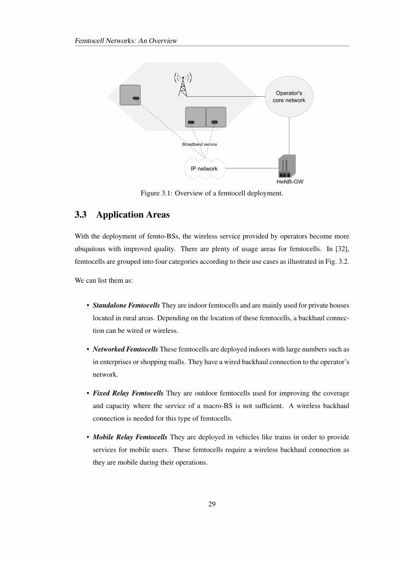
Femtocell Networks: An Overview
IP network
Operator'score network
HeNB-GW
Broadband service
Figure 3.1: Overview of a femtocell deployment.
3.3 Application Areas
With the deployment of femto-BSs, the wireless service provided by operators become more
ubiquitous with improved quality. There are plenty of usage areas for femtocells. In [32],
femtocells are grouped into four categories according to their use cases as illustrated in Fig. 3.2.
We can list them as:
• Standalone Femtocells They are indoor femtocells and are mainly used for private houses
located in rural areas. Depending on the location of these femtocells, a backhaul connec-
tion can be wired or wireless.
• Networked Femtocells These femtocells are deployed indoors with large numbers such as
in enterprises or shopping malls. They have a wired backhaul connection to the operator’s
network.
• Fixed Relay Femtocells They are outdoor femtocells used for improving the coverage
and capacity where the service of a macro-BS is not sufficient. A wireless backhaul
connection is needed for this type of femtocells.
• Mobile Relay Femtocells They are deployed in vehicles like trains in order to provide
services for mobile users. These femtocells require a wireless backhaul connection as
they are mobile during their operations.
29
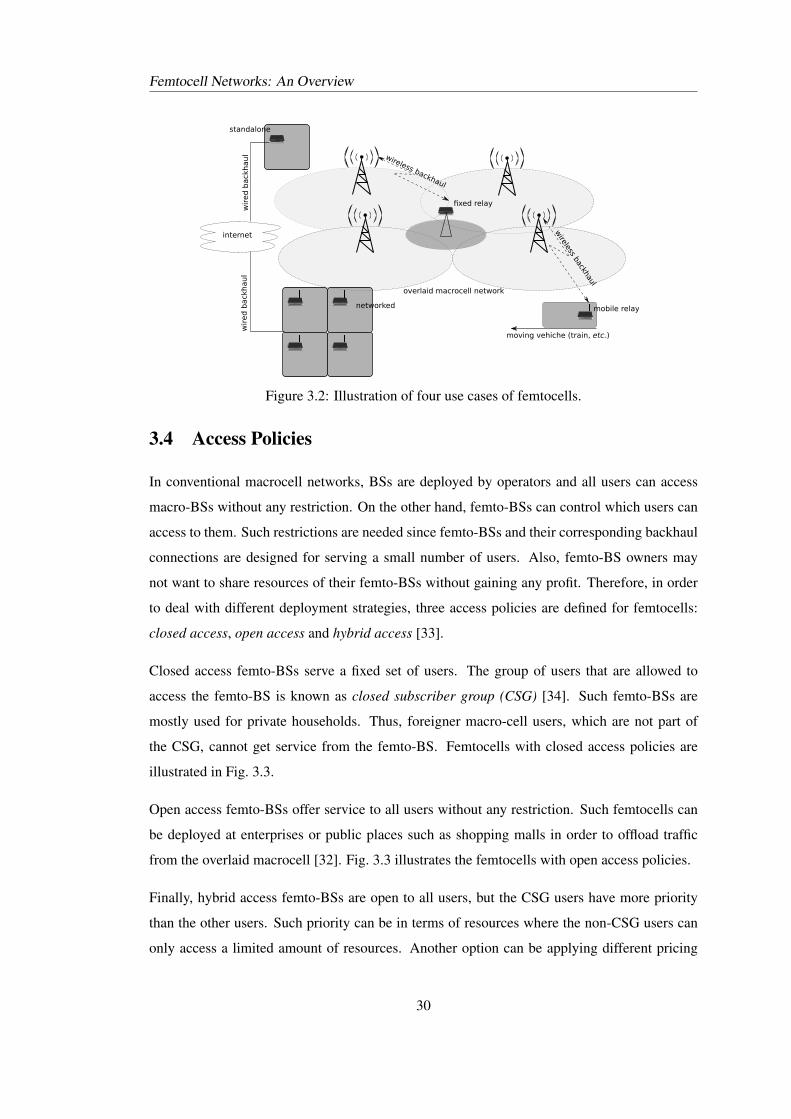
Femtocell Networks: An Overview
moving vehiche (train, etc.)
fixed relay
mobile relay
standalone
networked
internetw
ired b
ack
haul
wir
ed b
ack
haul wireless backhaul
wireless backhaul
overlaid macrocell network
Figure 3.2: Illustration of four use cases of femtocells.
3.4 Access Policies
In conventional macrocell networks, BSs are deployed by operators and all users can access
macro-BSs without any restriction. On the other hand, femto-BSs can control which users can
access to them. Such restrictions are needed since femto-BSs and their corresponding backhaul
connections are designed for serving a small number of users. Also, femto-BS owners may
not want to share resources of their femto-BSs without gaining any profit. Therefore, in order
to deal with different deployment strategies, three access policies are defined for femtocells:
closed access, open access and hybrid access [33].
Closed access femto-BSs serve a fixed set of users. The group of users that are allowed to
access the femto-BS is known as closed subscriber group (CSG) [34]. Such femto-BSs are
mostly used for private households. Thus, foreigner macro-cell users, which are not part of
the CSG, cannot get service from the femto-BS. Femtocells with closed access policies are
illustrated in Fig. 3.3.
Open access femto-BSs offer service to all users without any restriction. Such femtocells can
be deployed at enterprises or public places such as shopping malls in order to offload traffic
from the overlaid macrocell [32]. Fig. 3.3 illustrates the femtocells with open access policies.
Finally, hybrid access femto-BSs are open to all users, but the CSG users have more priority
than the other users. Such priority can be in terms of resources where the non-CSG users can
only access a limited amount of resources. Another option can be applying different pricing
30
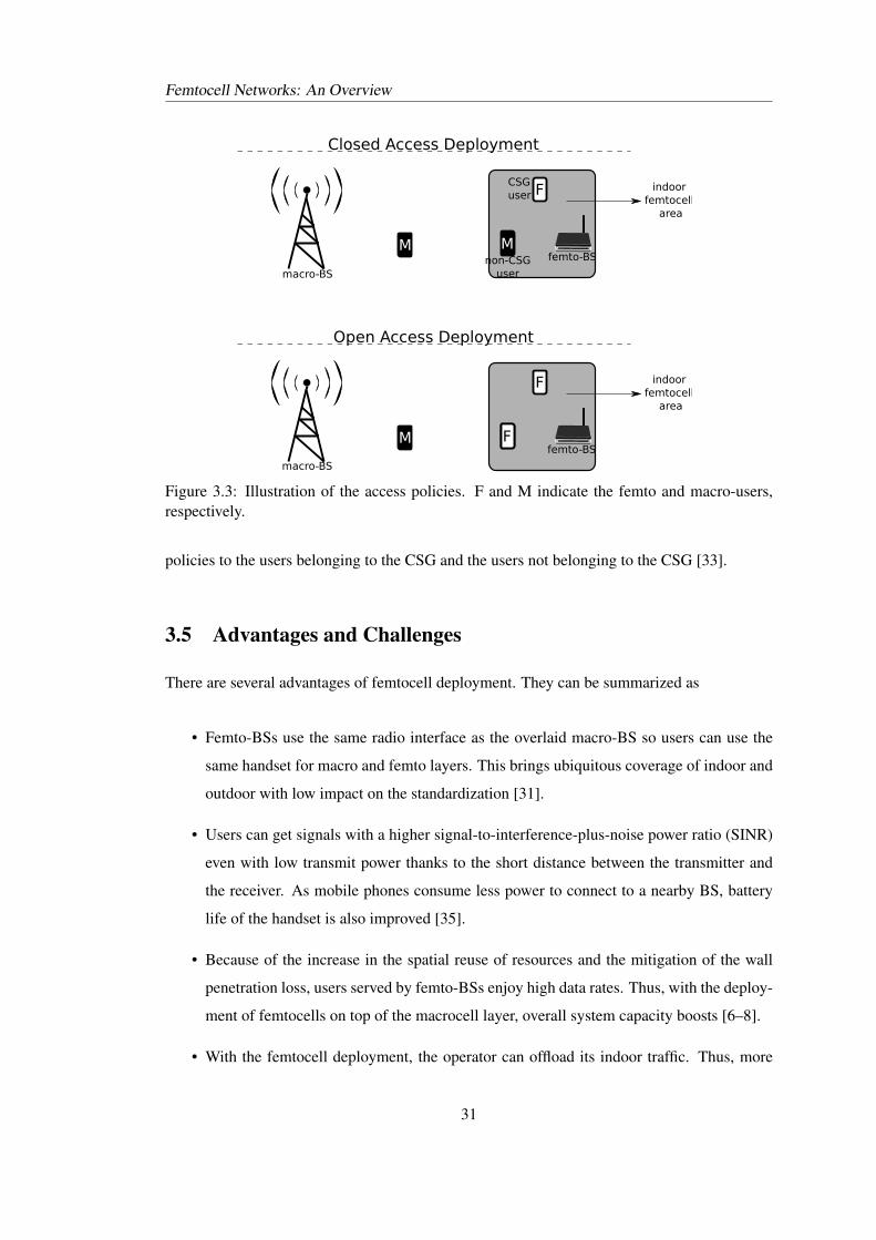
Femtocell Networks: An Overview
indoor femtocell
area
Open Access Deployment
F
M MF
Closed Access Deployment
F
M Mfemto-BS
femto-BS
macro-BS
macro-BS
indoor femtocell
area
CSGuser
non-CSGuser
Figure 3.3: Illustration of the access policies. F and M indicate the femto and macro-users,respectively.
policies to the users belonging to the CSG and the users not belonging to the CSG [33].
3.5 Advantages and Challenges
There are several advantages of femtocell deployment. They can be summarized as
• Femto-BSs use the same radio interface as the overlaid macro-BS so users can use the
same handset for macro and femto layers. This brings ubiquitous coverage of indoor and
outdoor with low impact on the standardization [31].
• Users can get signals with a higher signal-to-interference-plus-noise power ratio (SINR)
even with low transmit power thanks to the short distance between the transmitter and
the receiver. As mobile phones consume less power to connect to a nearby BS, battery
life of the handset is also improved [35].
• Because of the increase in the spatial reuse of resources and the mitigation of the wall
penetration loss, users served by femto-BSs enjoy high data rates. Thus, with the deploy-
ment of femtocells on top of the macrocell layer, overall system capacity boosts [6–8].
• With the femtocell deployment, the operator can offload its indoor traffic. Thus, more
31
Femtocell Networks: An Overview
resources can be assigned to outdoor users resulting in an improvement of their perfor-
mance [6, 35].
• Deployment of femto-BSs eventually decreases the need for further macro-BS deploy-
ment. This is an efficient solution for operators in terms of operation costs as the cost
of a femto-BS deployment is much lower than a macro-BS deployment. The cost of a
macro-BS to an operator does not only include hardware costs but also comprises leasing,
backhaul and electricity costs. On the other hand, the operator does not pay for leasing
or electricity to operate a femto-BS. Also, the price of a femto-BS is partly paid by an
end user. Therefore, femtocell deployments reduce the cost of operators [6, 23, 35].
• Deploying small cells reduces the overall energy consumption and yields to energy effi-
cient networks [36, 37].
Initially, femtocells were thought to be deployed only for coverage solutions under the control
of operators instead of mass market production. However, the increased effort on standardiza-
tion positively affects the commercialization of femto-BSs [38]. It is estimated that the number
of femto-BSs in the market will be around 60 million by 2015 [9], whereas there were 2.3 mil-
lion femto-BSs at the end of 2010 [39]. Such dense deployment of femto-BSs clearly comes
with challenges that can be listed as
• The most serious and detrimental problem arising with the introduction of femto-BSs is
the increase in interference. Interference mitigation requires extra attention especially
in networks where BSs are densely deployed. Detailed explanation of interference in
femtocell networks is given in Chapter 4.
• Femto-BSs’ transmission times should be aligned with macro-BSs in order to minimize
multi-access interference and achieve proper handover between layers.
• Since these devices have a plug-and-play nature, femtocells should self-optimize and
configure their parameters according to their dynamic environments.
• The backhaul service provided by broadband technology is not as advanced as the back-
haul used for macro-BSs. For instance, the delay performance of macrocell networks
cannot be achieved by the current broadband service. Also, the performance of the back-
haul service is limited if another broadband-based service such as Wi-Fi is concurrently
used with femto-BSs.
32
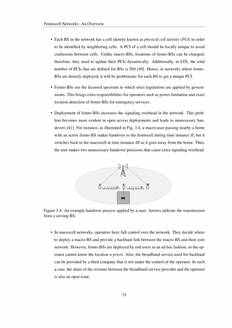
Femtocell Networks: An Overview
• Each BS in the network has a cell identity known as physical cell identity (PCI) in order
to be identified by neighboring cells. A PCI of a cell should be locally unique to avoid
confusions between cells. Unlike macro-BSs, locations of femto-BSs can be changed;
therefore, they need to update their PCIs dynamically. Additionally, in LTE, the total
number of PCIs that are defined for BSs is 504 [40]. Hence, in networks where femto-
BSs are densely deployed, it will be problematic for each BS to get a unique PCI.
• Femto-BSs use the licensed spectrum to which strict regulations are applied by govern-
ments. This brings extra responsibilities for operators such as power limitation and exact
location detection of femto-BSs for emergency services.
• Deployment of femto-BSs increases the signaling overhead in the network. This prob-
lem becomes more evident in open access deployments and leads to unnecessary han-
dovers [41]. For instance, as illustrated in Fig. 3.4, a macro-user passing nearby a home
with an active femto-BS makes handover to the femtocell during time instance II, but it
switches back to the macrocell at time instance III as it goes away from the home. Thus,
the user makes two unnecessary handover processes that cause extra signaling overhead.
moving direction moving direction
I II III
Figure 3.4: An example handover process applied by a user. Arrows indicate the transmissionfrom a serving BS.
• In macrocell networks, operators have full control over the network. They decide where
to deploy a macro-BS and provide a backhaul link between the macro-BS and their core
network. However, femto-BSs are deployed by end users in an ad hoc fashion, so the op-
erator cannot know the location a priori. Also, the broadband service used for backhaul
can be provided by a third company that is not under the control of the operator. In such
a case, the share of the revenue between the broadband service provider and the operator
is also an open issue.
33
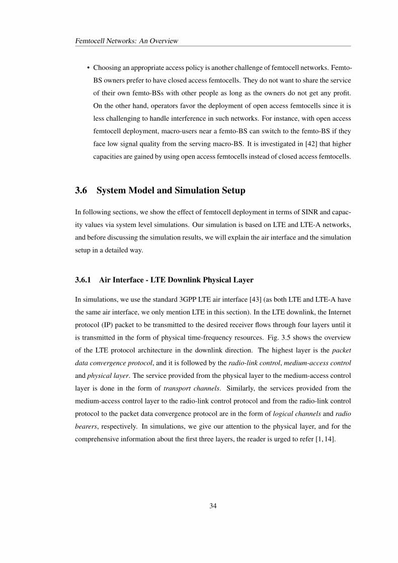
Femtocell Networks: An Overview
• Choosing an appropriate access policy is another challenge of femtocell networks. Femto-
BS owners prefer to have closed access femtocells. They do not want to share the service
of their own femto-BSs with other people as long as the owners do not get any profit.
On the other hand, operators favor the deployment of open access femtocells since it is
less challenging to handle interference in such networks. For instance, with open access
femtocell deployment, macro-users near a femto-BS can switch to the femto-BS if they
face low signal quality from the serving macro-BS. It is investigated in [42] that higher
capacities are gained by using open access femtocells instead of closed access femtocells.
3.6 System Model and Simulation Setup
In following sections, we show the effect of femtocell deployment in terms of SINR and capac-
ity values via system level simulations. Our simulation is based on LTE and LTE-A networks,
and before discussing the simulation results, we will explain the air interface and the simulation
setup in a detailed way.
3.6.1 Air Interface - LTE Downlink Physical Layer
In simulations, we use the standard 3GPP LTE air interface [43] (as both LTE and LTE-A have
the same air interface, we only mention LTE in this section). In the LTE downlink, the Internet
protocol (IP) packet to be transmitted to the desired receiver flows through four layers until it
is transmitted in the form of physical time-frequency resources. Fig. 3.5 shows the overview
of the LTE protocol architecture in the downlink direction. The highest layer is the packet
data convergence protocol, and it is followed by the radio-link control, medium-access control
and physical layer. The service provided from the physical layer to the medium-access control
layer is done in the form of transport channels. Similarly, the services provided from the
medium-access control layer to the radio-link control protocol and from the radio-link control
protocol to the packet data convergence protocol are in the form of logical channels and radio
bearers, respectively. In simulations, we give our attention to the physical layer, and for the
comprehensive information about the first three layers, the reader is urged to refer [1, 14].
34
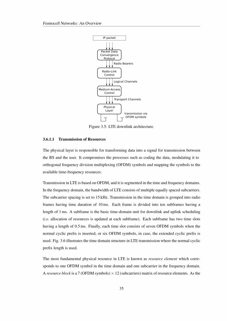
Femtocell Networks: An Overview
Packet Data Convergence
Protocol
Radio-LinkControl
Medium-AccessControl
Physical Layer
IP packet
transmission via OFDM symbols
Radio Bearers
Logical Channels
Transport Channels
Figure 3.5: LTE downlink architecture.
3.6.1.1 Transmission of Resources
The physical layer is responsible for transforming data into a signal for transmission between
the BS and the user. It compromises the processes such as coding the data, modulating it to
orthogonal frequency division multiplexing (OFDM) symbols and mapping the symbols to the
available time-frequency resources.
Transmission in LTE is based on OFDM, and it is segmented in the time and frequency domains.
In the frequency domain, the bandwidth of LTE consists of multiple equally spaced subcarriers.
The subcarrier spacing is set to 15 kHz. Transmission in the time domain is grouped into radio
frames having time duration of 10 ms. Each frame is divided into ten subframes having a
length of 1 ms. A subframe is the basic time-domain unit for downlink and uplink scheduling
(i.e. allocation of resources is updated at each subframe). Each subframe has two time slots
having a length of 0.5 ms. Finally, each time slot consists of seven OFDM symbols when the
normal cyclic prefix is inserted, or six OFDM symbols, in case, the extended cyclic prefix is
used. Fig. 3.6 illustrates the time domain structure in LTE transmission where the normal cyclic
prefix length is used.
The most fundamental physical resource in LTE is known as resource element which corre-
sponds to one OFDM symbol in the time domain and one subcarrier in the frequency domain.
A resource block is a 7 (OFDM symbols)× 12 (subcarriers) matrix of resource elements. As the
35
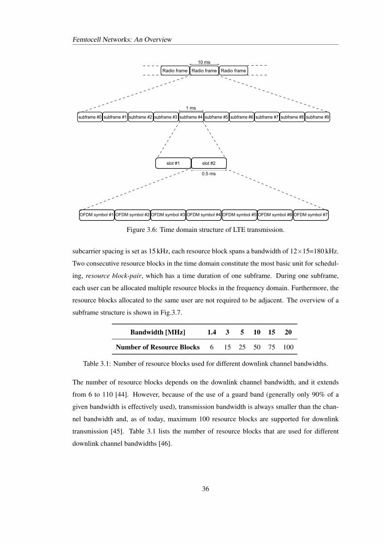
Femtocell Networks: An Overview
0.5tmst
Radiotframet
10tmst
Radiotframet Radiotframet
1tmst
subframet#7t subframet#8t subframet#9tsubframet#4t subframet#5t subframet#6tsubframet#3tsubframet#0t subframet#1t subframet#2t
OFDMtsymbolt#2tOFDMtsymbolt#1t OFDMtsymbolt#4tOFDMtsymbolt#3t OFDMtsymbolt#6tOFDMtsymbolt#5t OFDMtsymbolt#7t
slott#1t slott#2t
Figure 3.6: Time domain structure of LTE transmission.
subcarrier spacing is set as 15 kHz, each resource block spans a bandwidth of 12×15=180 kHz.
Two consecutive resource blocks in the time domain constitute the most basic unit for schedul-
ing, resource block-pair, which has a time duration of one subframe. During one subframe,
each user can be allocated multiple resource blocks in the frequency domain. Furthermore, the
resource blocks allocated to the same user are not required to be adjacent. The overview of a
subframe structure is shown in Fig.3.7.
Bandwidth [MHz] 1.4 3 5 10 15 20
Number of Resource Blocks 6 15 25 50 75 100
Table 3.1: Number of resource blocks used for different downlink channel bandwidths.
The number of resource blocks depends on the downlink channel bandwidth, and it extends
from 6 to 110 [44]. However, because of the use of a guard band (generally only 90% of a
given bandwidth is effectively used), transmission bandwidth is always smaller than the chan-
nel bandwidth and, as of today, maximum 100 resource blocks are supported for downlink
transmission [45]. Table 3.1 lists the number of resource blocks that are used for different
downlink channel bandwidths [46].
36
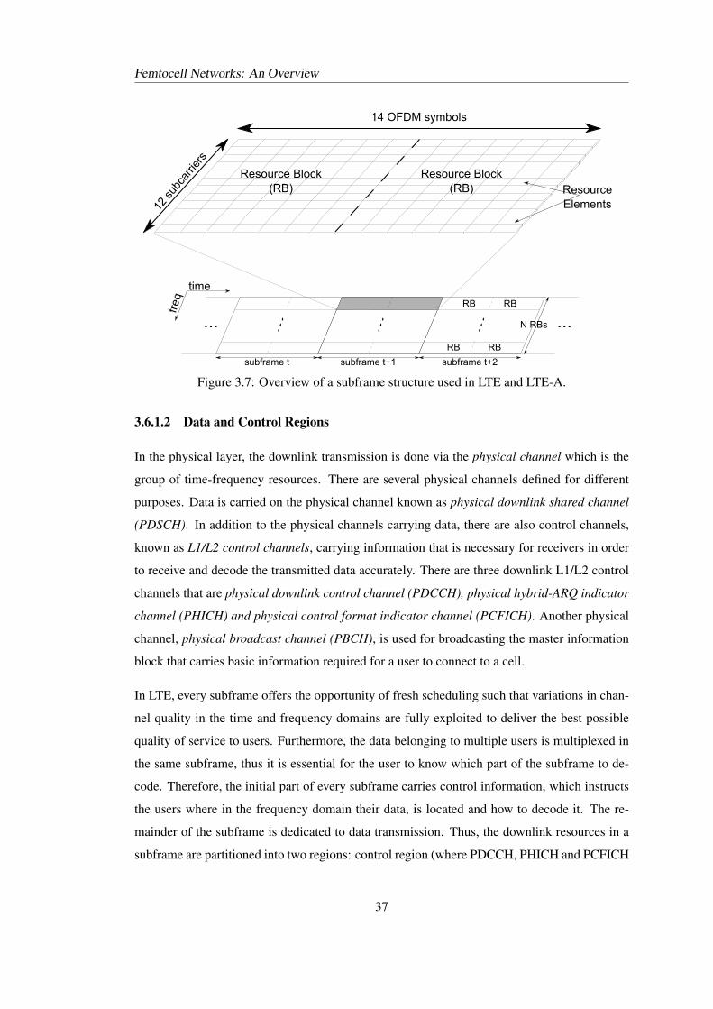
Femtocell Networks: An Overview
... ...
subframeMt subframeMt+1 subframeMt+2
time
freq
ResourceMElements
...
...
...
ResourceMBlock(RB)
ResourceMBlock(RB)
RB RB
RBRB
NMRBs
12Ms
ubca
rrier
s
14MOFDMMsymbols
Figure 3.7: Overview of a subframe structure used in LTE and LTE-A.
3.6.1.2 Data and Control Regions
In the physical layer, the downlink transmission is done via the physical channel which is the
group of time-frequency resources. There are several physical channels defined for different
purposes. Data is carried on the physical channel known as physical downlink shared channel
(PDSCH). In addition to the physical channels carrying data, there are also control channels,
known as L1/L2 control channels, carrying information that is necessary for receivers in order
to receive and decode the transmitted data accurately. There are three downlink L1/L2 control
channels that are physical downlink control channel (PDCCH), physical hybrid-ARQ indicator
channel (PHICH) and physical control format indicator channel (PCFICH). Another physical
channel, physical broadcast channel (PBCH), is used for broadcasting the master information
block that carries basic information required for a user to connect to a cell.
In LTE, every subframe offers the opportunity of fresh scheduling such that variations in chan-
nel quality in the time and frequency domains are fully exploited to deliver the best possible
quality of service to users. Furthermore, the data belonging to multiple users is multiplexed in
the same subframe, thus it is essential for the user to know which part of the subframe to de-
code. Therefore, the initial part of every subframe carries control information, which instructs
the users where in the frequency domain their data, is located and how to decode it. The re-
mainder of the subframe is dedicated to data transmission. Thus, the downlink resources in a
subframe are partitioned into two regions: control region (where PDCCH, PHICH and PCFICH
37
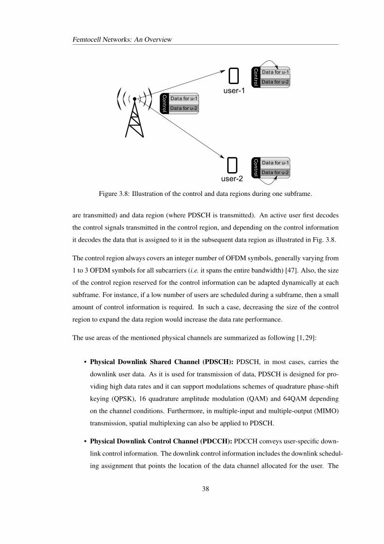
Femtocell Networks: An Overview
Co
ntro
l
Data for u-1
Data for u-2
user-1
user-2
Co
ntro
l
Data for u-1
Data for u-2
Co
ntro
l
Data for u-1
Data for u-2
Figure 3.8: Illustration of the control and data regions during one subframe.
are transmitted) and data region (where PDSCH is transmitted). An active user first decodes
the control signals transmitted in the control region, and depending on the control information
it decodes the data that is assigned to it in the subsequent data region as illustrated in Fig. 3.8.
The control region always covers an integer number of OFDM symbols, generally varying from
1 to 3 OFDM symbols for all subcarriers (i.e. it spans the entire bandwidth) [47]. Also, the size
of the control region reserved for the control information can be adapted dynamically at each
subframe. For instance, if a low number of users are scheduled during a subframe, then a small
amount of control information is required. In such a case, decreasing the size of the control
region to expand the data region would increase the data rate performance.
The use areas of the mentioned physical channels are summarized as following [1, 29]:
• Physical Downlink Shared Channel (PDSCH): PDSCH, in most cases, carries the
downlink user data. As it is used for transmission of data, PDSCH is designed for pro-
viding high data rates and it can support modulations schemes of quadrature phase-shift
keying (QPSK), 16 quadrature amplitude modulation (QAM) and 64QAM depending
on the channel conditions. Furthermore, in multiple-input and multiple-output (MIMO)
transmission, spatial multiplexing can also be applied to PDSCH.
• Physical Downlink Control Channel (PDCCH): PDCCH conveys user-specific down-
link control information. The downlink control information includes the downlink schedul-
ing assignment that points the location of the data channel allocated for the user. The
38
Femtocell Networks: An Overview
downlink control information also includes the uplink scheduling grants and power-
control commands. Different downlink control information formats having different sizes
are defined depending on the control information carried in it.
• Physical Hybrid-ARQ Indicator Channel (PHICH): It indicates whether the BS has
received the uplink data correctly.
• Physical Control Format Indicator Channel (PCFICH): It tells the users about the
size of the control region in terms of the number of OFDM symbols. Based on this
information, users in the cell can know from which OFDM symbol, the data region starts.
There is only one PCFICH for a given cell that is same for all users served by it. PCFICH
is always mapped to the first OFDM symbol of each subframe as the size of the control
region is not known until the PCFICH is decoded.
• Physical Broadcast Channel (PBCH): Unlike other physical channels, PBCH is broad-
cast periodically at every 10 ms frame. It conveys information such as system bandwidth
that is required for a user to decode other physical channels.
Because of their essential role in reliable data transmission, the correct decoding of control
signals (PDCCH, PHICH and PCFICH) is crucial for users. It must be noted that the data
contained in a subframe will be lost if the control information is not correctly decoded and the
user goes into outage. For instance, in order to get its dedicated data, a user should decode the
PDCCH precisely. If it is not received correctly, the data transmission also fails. Therefore,
unlike physical channels carrying data, the utmost importance for the control channels is the
robustness. Only with reliable transmission of the control channels, the cell can achieve sub-
stantial coverage. In order to make the transmitted control signals decodable even under high
interference conditions, they are spread over the available frequency range to increase the diver-
sity. Also, low order modulation schemes are used for these signals independent of the channel
conditions, i.e., for PDCCH and PCFICH, QPSK is used and for PHICH binary phase-shift
keying (BPSK) is applied.
In addition to the physical channels, a BS also transmits periodic signals known as downlink
signals. Downlink signals are grouped into two classes; synchronization signals and reference
signals [1, 29].
• Synchronization Signals: There are two types of synchronization signals; primary
39
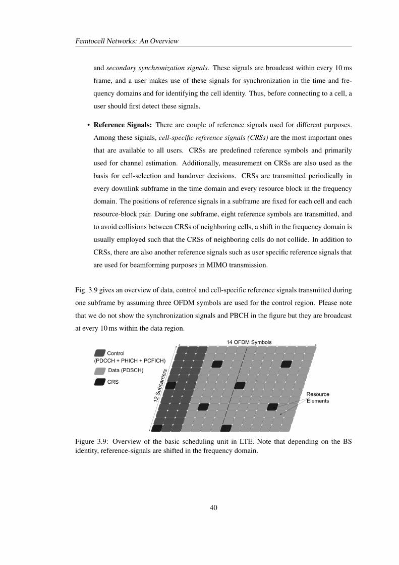
Femtocell Networks: An Overview
and secondary synchronization signals. These signals are broadcast within every 10 ms
frame, and a user makes use of these signals for synchronization in the time and fre-
quency domains and for identifying the cell identity. Thus, before connecting to a cell, a
user should first detect these signals.
• Reference Signals: There are couple of reference signals used for different purposes.
Among these signals, cell-specific reference signals (CRSs) are the most important ones
that are available to all users. CRSs are predefined reference symbols and primarily
used for channel estimation. Additionally, measurement on CRSs are also used as the
basis for cell-selection and handover decisions. CRSs are transmitted periodically in
every downlink subframe in the time domain and every resource block in the frequency
domain. The positions of reference signals in a subframe are fixed for each cell and each
resource-block pair. During one subframe, eight reference symbols are transmitted, and
to avoid collisions between CRSs of neighboring cells, a shift in the frequency domain is
usually employed such that the CRSs of neighboring cells do not collide. In addition to
CRSs, there are also another reference signals such as user specific reference signals that
are used for beamforming purposes in MIMO transmission.
Fig. 3.9 gives an overview of data, control and cell-specific reference signals transmitted during
one subframe by assuming three OFDM symbols are used for the control region. Please note
that we do not show the synchronization signals and PBCH in the figure but they are broadcast
at every 10 ms within the data region.
14IOFDMISymbols
12IS
ubca
rrie
rs
ResourceIElements
ControlI
DataI(PDSCH)
CRS
(PDCCHI+IPHICHI+IPCFICH)
Figure 3.9: Overview of the basic scheduling unit in LTE. Note that depending on the BSidentity, reference-signals are shifted in the frequency domain.
40
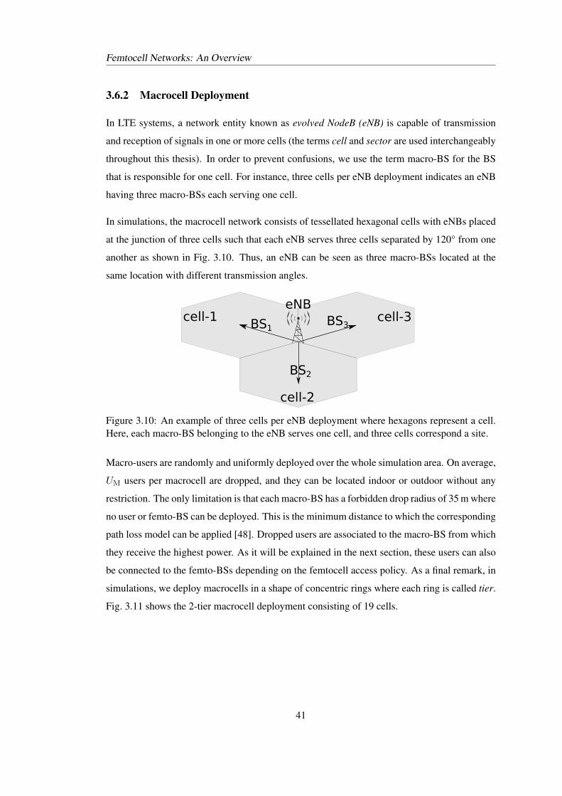
Femtocell Networks: An Overview
3.6.2 Macrocell Deployment
In LTE systems, a network entity known as evolved NodeB (eNB) is capable of transmission
and reception of signals in one or more cells (the terms cell and sector are used interchangeably
throughout this thesis). In order to prevent confusions, we use the term macro-BS for the BS
that is responsible for one cell. For instance, three cells per eNB deployment indicates an eNB
having three macro-BSs each serving one cell.
In simulations, the macrocell network consists of tessellated hexagonal cells with eNBs placed
at the junction of three cells such that each eNB serves three cells separated by 120° from one
another as shown in Fig. 3.10. Thus, an eNB can be seen as three macro-BSs located at the
same location with different transmission angles.
eNB
BS1
BS2
BS3cell-1
cell-2
cell-3
Figure 3.10: An example of three cells per eNB deployment where hexagons represent a cell.Here, each macro-BS belonging to the eNB serves one cell, and three cells correspond a site.
Macro-users are randomly and uniformly deployed over the whole simulation area. On average,
UM users per macrocell are dropped, and they can be located indoor or outdoor without any
restriction. The only limitation is that each macro-BS has a forbidden drop radius of 35 m where
no user or femto-BS can be deployed. This is the minimum distance to which the corresponding
path loss model can be applied [48]. Dropped users are associated to the macro-BS from which
they receive the highest power. As it will be explained in the next section, these users can also
be connected to the femto-BSs depending on the femtocell access policy. As a final remark, in
simulations, we deploy macrocells in a shape of concentric rings where each ring is called tier.
Fig. 3.11 shows the 2-tier macrocell deployment consisting of 19 cells.
41
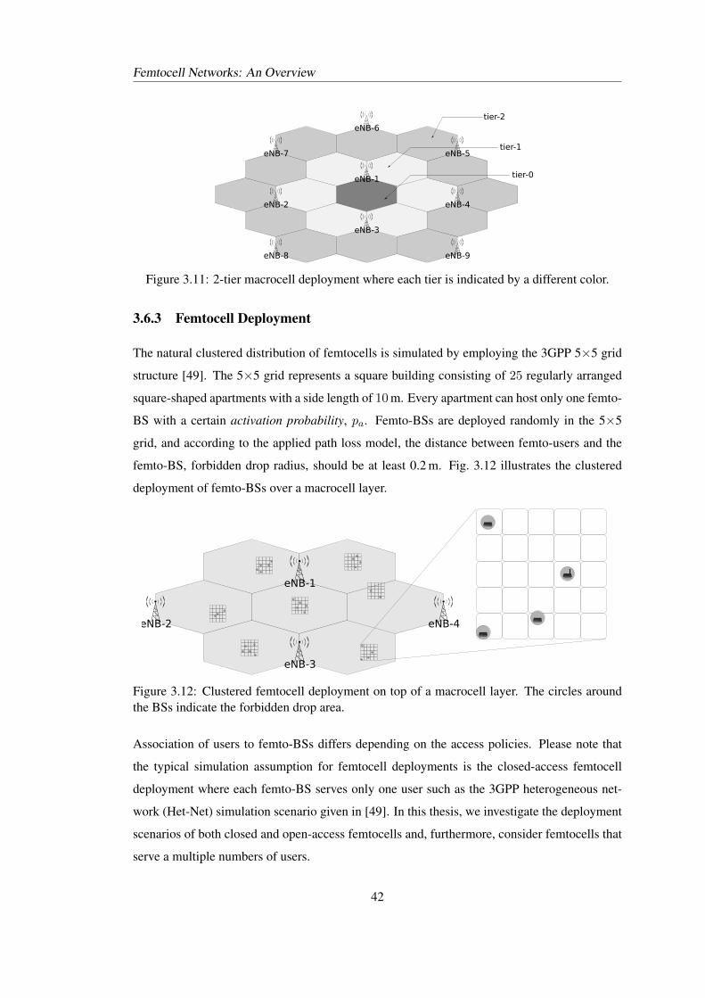
Femtocell Networks: An Overview
eNB-1
eNB-2
eNB-3
eNB-4
eNB-5
eNB-6
eNB-7
eNB-8 eNB-9
tier-2
tier-0
tier-1
Figure 3.11: 2-tier macrocell deployment where each tier is indicated by a different color.
3.6.3 Femtocell Deployment
The natural clustered distribution of femtocells is simulated by employing the 3GPP 5×5 grid
structure [49]. The 5×5 grid represents a square building consisting of 25 regularly arranged
square-shaped apartments with a side length of 10 m. Every apartment can host only one femto-
BS with a certain activation probability, pa. Femto-BSs are deployed randomly in the 5×5
grid, and according to the applied path loss model, the distance between femto-users and the
femto-BS, forbidden drop radius, should be at least 0.2 m. Fig. 3.12 illustrates the clustered
deployment of femto-BSs over a macrocell layer.
eNB-1
eNB-2
eNB-3
eNB-4
Figure 3.12: Clustered femtocell deployment on top of a macrocell layer. The circles aroundthe BSs indicate the forbidden drop area.
Association of users to femto-BSs differs depending on the access policies. Please note that
the typical simulation assumption for femtocell deployments is the closed-access femtocell
deployment where each femto-BS serves only one user such as the 3GPP heterogeneous net-
work (Het-Net) simulation scenario given in [49]. In this thesis, we investigate the deployment
scenarios of both closed and open-access femtocells and, furthermore, consider femtocells that
serve a multiple numbers of users.
42
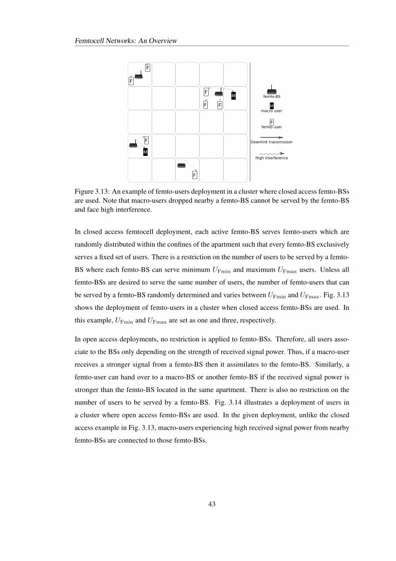
Femtocell Networks: An Overview
M
F
M
F
F
F
F
F
F
femto-BS
Mmacro user
Ffemto user
High interference
Downlink transmission
Figure 3.13: An example of femto-users deployment in a cluster where closed access femto-BSsare used. Note that macro-users dropped nearby a femto-BS cannot be served by the femto-BSand face high interference.
In closed access femtocell deployment, each active femto-BS serves femto-users which are
randomly distributed within the confines of the apartment such that every femto-BS exclusively
serves a fixed set of users. There is a restriction on the number of users to be served by a femto-
BS where each femto-BS can serve minimum UFmin and maximum UFmax users. Unless all
femto-BSs are desired to serve the same number of users, the number of femto-users that can
be served by a femto-BS randomly determined and varies between UFmin and UFmax. Fig. 3.13
shows the deployment of femto-users in a cluster when closed access femto-BSs are used. In
this example, UFmin and UFmax are set as one and three, respectively.
In open access deployments, no restriction is applied to femto-BSs. Therefore, all users asso-
ciate to the BSs only depending on the strength of received signal power. Thus, if a macro-user
receives a stronger signal from a femto-BS then it assimilates to the femto-BS. Similarly, a
femto-user can hand over to a macro-BS or another femto-BS if the received signal power is
stronger than the femto-BS located in the same apartment. There is also no restriction on the
number of users to be served by a femto-BS. Fig. 3.14 illustrates a deployment of users in
a cluster where open access femto-BSs are used. In the given deployment, unlike the closed
access example in Fig. 3.13, macro-users experiencing high received signal power from nearby
femto-BSs are connected to those femto-BSs.
43
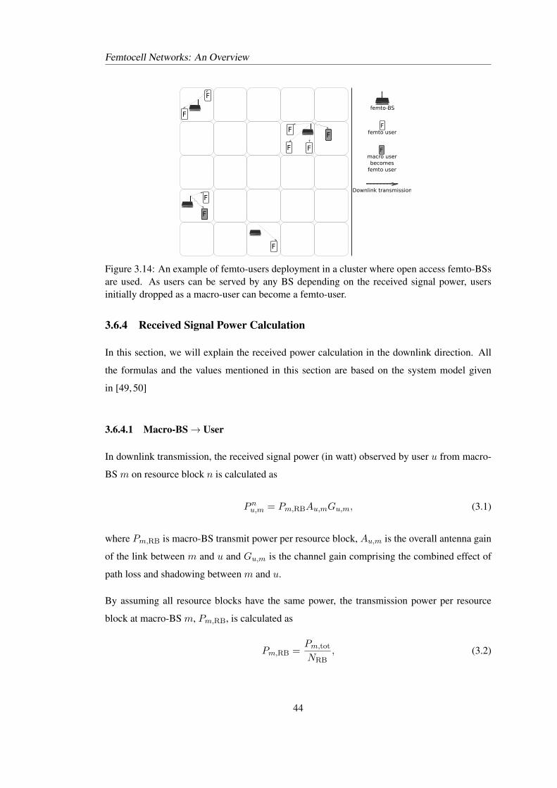
Femtocell Networks: An Overview
femto-BS
Ffemto user
Downlink transmission
Fmacro userbecomes
femto user
M
F
M
F
F
F
F
F
F
F
F
Figure 3.14: An example of femto-users deployment in a cluster where open access femto-BSsare used. As users can be served by any BS depending on the received signal power, usersinitially dropped as a macro-user can become a femto-user.
3.6.4 Received Signal Power Calculation
In this section, we will explain the received power calculation in the downlink direction. All
the formulas and the values mentioned in this section are based on the system model given
in [49, 50]
3.6.4.1 Macro-BS→ User
In downlink transmission, the received signal power (in watt) observed by user u from macro-
BS m on resource block n is calculated as
Pnu,m = Pm,RBAu,mGu,m, (3.1)
where Pm,RB is macro-BS transmit power per resource block, Au,m is the overall antenna gain
of the link between m and u and Gu,m is the channel gain comprising the combined effect of
path loss and shadowing between m and u.
By assuming all resource blocks have the same power, the transmission power per resource
block at macro-BS m, Pm,RB, is calculated as
Pm,RB =Pm,tot
NRB, (3.2)
44
Femtocell Networks: An Overview
where Pm,tot is the macro-BS total transmit power and NRB is the total number of resource
blocks.
As an antenna model, two-dimensional horizontal model with a directional antenna is used. In
such a model, the gain of an antenna decreases as the user goes away from the main radiation
direction of the antenna. Thus, the gain of an antenna depends on the radiation pattern of the
antenna and the position of the user according to the antenna [51]. The overall antenna gain
Au,m is calculated as
Au,m = 10(Am−Au,m(θ))/10, (3.3)
where Am is the maximum gain of an antenna over an isotropic antenna given in dBi, Au,m(θ)
is the loss in the antenna gain according to the horizontal pattern of the antenna and the location
of the user with respect to the antenna. The azimuth antenna pattern is calculated as:
Au,m (θ) = min
[12
(θu,mθ3dB
)2
, Af2b
], (3.4)
where θu,m is the horizontal angle between user u and macro-BS m, θ3dB is the half power
beam width indicating the angular distance on the main lobe where the antenna gain becomes
half of the maximum value (in decibel−3 dB) and Af2b is the antenna front to back ratio which
stands for the ratio of the gain from the front side to the back side of the antenna.
The channel gain Gu,m takes the effect of path loss and shadowing and is measured as
Gu,m = 10−(PLu,m+Xσ)/10, (3.5)
where PLu,m is the path loss in dB between u and m and Xσ is the shadowing effect. The
path loss model used in the simulation is based on the model defined in [49]. For 2 GHz carrier
frequency, the path loss between the macro-BS m and the user u located outside is calculated
as
PLu,m[dB] = 15.3 + 37.6log10 (du,m) , (3.6)
where du,m is the distance (in m) between u and m. For the links between the macro-BS
and users located indoors, the wall penetration loss should also be included in the path loss
calculation as
PLu,m[dB] = 15.3 + 37.6log10 (du,m) + Lwall, (3.7)
45
Femtocell Networks: An Overview
where Lwall is the wall penetration loss in dB.
In order to include the effect of shadowing, for all links between macro-BSs and users, a log-
normal distributed shadowing value, Xσ is added to the received signal power calculation. Xσ
is a random variable having a zero-mean Gaussian distribution (in dB) with a standard deviation
σ. Shadowing values generated for links between BSs and users are correlated with each other.
Correlation values vary between 0 and 1. Correlation value 0 indicates there is no correlation
between the shadowing values of the different BSs, and 1 implies that the shadowing values are
entirely alike.
3.6.4.2 Femto-BS→ User
In downlink transmission, the received signal power (in watt) observed by user u from femto-
BS f on resource block n is calculated as
Pnu,f = Pf,RBAu,fGu,f , (3.8)
where Pf,RB is femto-BS transmit power per resource block, Au,f is the overall antenna gain
of the link between f and u and Gu,f is the channel gain comprising the combined effect of
path loss and shadowing between f and u.
By assuming all resource blocks have the same power, the transmission power per resource
block at femto-BS f , Pf,RB, is calculated as
Pf,RB =Pf,tot
NRB, (3.9)
where Pf,tot is the femto-BS total transmit power and NRB is the total number of resource
blocks.
Unlike macro-BSs, omnidirectional antennas are used for femto-BSs. Thus, the loss according
to the antenna pattern is not involved in Au,f . In other words
Au,f = 10Af/10, (3.10)
where Af is the femto-BS antenna gain in dBi.
46
Femtocell Networks: An Overview
The channel gain Gu,f takes the effect of path loss and shadowing and is measured as
Gu,f = 10−(PLu,f+Xσ)/10, (3.11)
where PLu,f is the path loss between u and f and Xσ is the shadowing effect. The path loss
model used in the simulation is based on the model defined in [49]. The path loss between
femto-BS f and user u located in the same 5×5 grid is calculated as
PLu,f [dB] = 37 + 30log10 (du,f ) , (3.12)
where du,f is the distance (in m) between f and u. This is a simplified path loss model used
for 5×5 deployments, and it also includes the wall penetration loss. For the links between a
femto-BS and a user located outside the grid, the external wall penetration loss should also be
included in the path loss calculation as
PLu,f [dB] = 15.3 + 37.6log10 (du,f ) + Lwall, (3.13)
Similar to macro-BSs, the log-normal shadowing is added to all links between femto-BSs and
users.
3.6.5 SINR and Capacity Calculation
The SINR of resource block n experienced by user u served by BS b is calculated as:
γnu =Pnu,b∑
i∈IuPnu,i + ηRB
, (3.14)
where Pnu,b is the received signal power from the serving BS, Pnu,i is the interfering power from
BS i, Iu is the set of interfering BSs (both femto and macro-BSs) and ηRB is the sum effect of
the thermal noise and receiver noise at the user side over the bandwidth of one resource block.
The total noise power over a resource block is calculated (in Watt) as
ηRB = BRB ×N0 × 10NFU/10, (3.15)
whereBRB is the bandwidth of a resource block,N0 is the thermal noise power spectral density
47
Femtocell Networks: An Overview
in W/Hz and NFU is the user noise figure in dB. The noise figure indicates the ratio of the
thermal noise at the receiver of the user to the ideal receiver. Note that the noise power spectral
density over each resource block is assumed to be same.
When we plot the cumulative distribution function (CDF) of the SINR of users, we use the
average SINR experienced by users and it is calculated as
γu =
∑n∈Nu
γnu
|Nu|, (3.16)
where Nu is the set of resource blocks scheduled to u and γnu is the SINR of resource block n
experienced by u.
For throughput calculations, the attenuated and truncated Shannon bound method is used [52].
It gives the capacity of a channel with link adaptation, which means that the modulation and
coding schemes are selected based on SINRs. Given a specific SINR of user u on resource
block n, γnu , the spectral efficiency of user u on resource block n in [bps/Hz] is calculated
as [52]:
Rnu =
0 for γnu [dB] < −10
0.6log2(1 + γnu ) for −10 6 γnu [dB] 6 22
4.4 for γnu [dB] > 22
(3.17)
where 0.6 is the attenuation factor which represents implementation losses, −10 and 22 are the
minimum and maximum SINRs [in dB] used by the available modulation and coding schemes.
According to (3.17), for SINR values less than −10 dB, no reliable data transmission can be
achieved, so the spectral efficiency becomes zero. For SINR values higher than 22 dB, no fur-
ther improvement in the spectral efficiency can be gained due to a limitation in the modulation
and coding schemes used in the system. Thus, the maximum achievable spectral efficiency is
limited to 4.4 bps/Hz that is obtained by putting 22 dB in (3.17).
One important point we should also consider is the minimum SINR value for proper decoding
of the control channels. Each control channel (PDCCH, PHICH and PCFICH) has different
minimum SINR threshold values in order to be received correctly [53, 54] because a particular
transmission process (i.e. modulation of the signals, mapping of the resources to the antennas)
is applied for each control channel [14]. In our simulation, we set an average value of−6 dB for
the minimum required SINR to decode the control channels. Thus, it is assumed that a user goes
into outage if it is not allocated any resource blocks having SINR above −6 dB. Therefore, as
48
Femtocell Networks: An Overview
we do not apply any particular control channel protection technique, the minimum SINR used
in (3.17) for the capacity calculation actually becomes −6 dB.
Given the set Nu of the resource blocks allocated to user u, the capacity Cu of user u amounts
to
Cu =∑n∈Nu
BeffBRBRnu, (3.18)
where BRB is the bandwidth of a resource block and Beff is the bandwidth efficiency. Because
of the control signals and cyclic prefix insertion, some portion of available resources cannot
be used for data transmission. Thus, in capacity calculations, we introduce the bandwidth
efficiency that is equal to
Beff = RCPRPDSCH, (3.19)
where RCP stands for the ratio of resources used for transmission after cyclic prefix insertion
and RPDSCH indicates the ratio of resource elements that are available for data transmission
(PDSCH) to all available resource elements after making allocation of the rest physical chan-
nels (PDCCH, PHICH, PCFICH and PBCH) and reference signals (CRSs and synchronization
signals).
When the normal cyclic prefix is applied, it introduces an overhead around 7.0%. Thus, RCP
amounts to 0.93 [29, 55]. RPDSCH depends on the bandwidth and the number of symbols
used for the control region. Table 3.2 lists RPDSCH according to varying bandwidth where the
control region consists of 3 symbols [29].
Bandwidth [MHz] 1.4 3 5 10 15 20
PDSCH Ratio 69.4% 72.8% 73.7% 74.3% 74.6% 74.7%
Table 3.2: Ratio of resource elements available for PDSCH transmission by assuming 3OFDMA symbol constitutes the control region.
3.6.6 Scheduling of Resource Blocks
In simulations, we assume that each user has an infinite queue length and a BS allocates all
available resources to its users. This kind of traffic is also known as full-buffer traffic. For
a scheduling strategy, the proportional-fair strategy is an ideal candidate since it is easy to
implement without considering the traffic requirements (as we assume full-buffer traffic), and
it exploits the multi-user diversity as well as offering fairness. However, the proportional-fair
49
Femtocell Networks: An Overview
scheduler needs a time window to calculate the average user data rate. On the other hand, our
simulation is based on snapshots with a duration of one subframe. For this purpose, we develop
a scheduler strategy similar to the proportional-fair scheduler but without using a time window.
In our system model, we assume that the serving BS gets feedback of the SINR of each subband
from each user. Thus, the scheduler can roughly calculate the corresponding data rate of a user
in a resource block for the next subframe, if it allocates the given resource block to that user.
Based on this information, assume the scheduler allocates resource blocks starting from the first
resource block, and given that the scheduler has allocated the resource blocks starting from the
first resource block until n, a resource block n is allocated to a user u according to
u = arg maxu∈U
Cnu
Cmax(u, n), (3.20)
where U is the set of users served by a same BS. Cnu represents the corresponding data rate that
user u would have in resource block n if n is allocated to u for the next subframe. Cmax(u, n)
denotes the maximum achievable data rate of user u for the next subframe if all available re-
source blocks are allocated to u. Cmax(u, n) is calculated as
Cmax(u, n) =∑
i∈Nu(n−1)
Ciu +∑
i∈Ncand(u)
i≥n
Ciu, (3.21)
where Nu(n− 1) is the set of resource blocks that are already allocated to u. As the scheduler
starts allocating resource blocks from the first resource block, at the instance of allocating
resource block n, the set of resource blocks allocated to each user until resource block n is
already known by the scheduler. Cmax(u, n) denotes the maximum potential sum data rate
that can be achieved by considering the resources blocks which are already assigned to u and
by allocating all remaining available resource blocks from n to N which belong to candidate
resource blocks that can be allocated to u,Ncand(u). In other words, first part of (3.21) indicates
the total achieved data rate of u according to the set resource blocks that are allocated to u.
Second part corresponds to the maximum achievable data rate for u if the rest resource blocks
that are available for u are allocated to it. Thus, the scheduling algorithm given in (3.20) is
a measure of how convenient the given resource block is for user u relative to other resource
blocks that can be allocated to user u.
By using the algorithm given in (3.20), the scheduler allocates a resource block to a user over
50
Femtocell Networks: An Overview
which the user experiences high capacity. Also, the scheduler prioritizes the users with low
data rates; thus, the fairness among users increases. In this way, we favor the selection of a user
with less available resources than other users. Such type of scheduling algorithm is essential
for resource partitioning methods which we will investigate throughout the next chapters where
users have a different amount of available resources that can be allocated to them.
3.7 Results
We use the Monte Carlo simulation consisting of snapshots. The simulation area is composed
of one tier of hexagonal cells; however, statistics are collected from the inner cell, namely tier-0.
We simulate the outer tier for eliminating the edge effects. At every snapshot of the simulator,
BSs and users are dropped over the simulation area, and users are associated to their serving
BSs depending on the access policies. The duration of each snapshot is set as the duration of
one subframe, therefore, during the snapshot, position and shadowing values of users do not
change.
We consider single-input and single-output (SISO) transmission where all BSs and users have
a single Rx and Tx antenna. The bandwidth of the system is 10 Mhz and it has 50 resource
blocks (50 resource blocks constitutes a bandwidth of 9 MHz, and the rest 1 MHz is used as
a guard band as aligned in Table 3.1). The bandwidth is assumed to be flat in the frequency
domain. Also, we assume that there is perfect synchronization in time and frequency that
prevents interference between neighboring resource blocks. We apply a normal cyclic prefix
where there are 7 orthogonal frequency division multiple access (OFDMA) symbols per slot,
and for each subframe we fix the control region at 3 symbols. Thus, we set Beff in (3.19) as
0.93× 0.743 ≈ 0.69. Full-buffer transmission is assumed where every BS assigns all available
resource blocks to its served users. This is the worst-case scenario in terms of interference since
all users and BSs are active.
The statistics such as the user SINR and capacity are measured at the end of each snapshot.
Calculation of the user SINR is done by averaging the SINRs of resource blocks that are allo-
cated to a user as given in (3.14) and (3.16). The user capacity is calculated by summing up the
capacities of resource blocks scheduled to it as given in (3.18). All the parameters used for the
simulation parameters are based on the LTE and LTE-A specifications [49,50] and summarized
in Table 3.3.
51
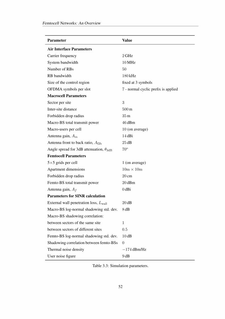
Femtocell Networks: An Overview
Parameter Value
Air Interface ParametersCarrier frequency 2 GHz
System bandwidth 10 MHz
Number of RBs 50
RB bandwidth 180 kHz
Size of the control region fixed at 3 symbols
OFDMA symbols per slot 7 - normal cyclic prefix is applied
Macrocell ParametersSector per site 3
Inter-site distance 500 m
Forbidden drop radius 35 m
Macro-BS total transmit power 46 dBm
Macro-users per cell 10 (on average)
Antenna gain, Am 14 dBi
Antenna front to back ratio, Af2b 25 dB
Angle spread for 3dB attenuation, θ3dB 70o
Femtocell Parameters5×5 grids per cell 1 (on average)
Apartment dimensions 10m× 10m
Forbidden drop radius 20 cm
Femto-BS total transmit power 20 dBm
Antenna gain, Af 0 dBi
Parameters for SINR calculationExternal wall penetration loss, Lwall 20 dB
Macro-BS log-normal shadowing std. dev. 8 dB
Macro-BS shadowing correlation:
between sectors of the same site 1
between sectors of different sites 0.5
Femto-BS log-normal shadowing std. dev. 10 dB
Shadowing correlation between femto-BSs 0
Thermal noise density −174 dBm/Hz
User noise figure 9 dB
Table 3.3: Simulation parameters.
52
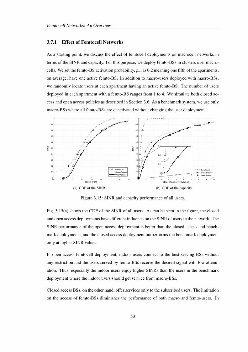
Femtocell Networks: An Overview
3.7.1 Effect of Femtocell Networks
As a starting point, we discuss the effect of femtocell deployments on macrocell networks in
terms of the SINR and capacity. For this purpose, we deploy femto-BSs in clusters over macro-
cells. We set the femto-BS activation probability, pa, as 0.2 meaning one fifth of the apartments,
on average, have one active femto-BS. In addition to macro-users deployed with macro-BSs,
we randomly locate users at each apartment having an active femto-BS. The number of users
deployed in each apartment with a femto-BS ranges from 1 to 4. We simulate both closed ac-
cess and open access policies as described in Section 3.6. As a benchmark system, we use only
macro-BSs where all femto-BSs are deactivated without changing the user deployment.
−10 −5 0 5 10 15 20 25 300
0.1
0.2
0.3
0.4
0.5
0.6
0.7
0.8
0.9
1
SINRl[dB]
CD
F
Benchmark
ClosedAccess
OpenAccess
(a) CDF of the SINR
0 1 2 3 4 5 6 7 8 9 100
0.1
0.2
0.3
0.4
0.5
0.6
0.7
0.8
0.9
1
User Capacity [Mbps]
CDF
Benchmark
ClosedAccess
OpenAccess0 0.5 10
0.1
0.2
0.3
(b) CDF of the capacity
Figure 3.15: SINR and capacity performance of all users.
Fig. 3.15(a) shows the CDF of the SINR of all users. As can be seen in the figure, the closed
and open access deployments have different influence on the SINR of users in the network. The
SINR performance of the open access deployment is better than the closed access and bench-
mark deployments, and the closed access deployment outperforms the benchmark deployment
only at higher SINR values.
In open access femtocell deployment, indoor users connect to the best serving BSs without
any restriction and the users served by femto-BSs receive the desired signal with low attenu-
ation. Thus, especially the indoor users enjoy higher SINRs than the users in the benchmark
deployment where the indoor users should get service from macro-BSs.
Closed access BSs, on the other hand, offer services only to the subscribed users. The limitation
on the access of femto-BSs diminishes the performance of both macro and femto-users. In
53
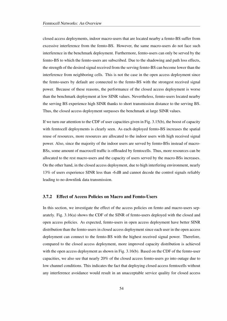
Femtocell Networks: An Overview
closed access deployments, indoor macro-users that are located nearby a femto-BS suffer from
excessive interference from the femto-BS. However, the same macro-users do not face such
interference in the benchmark deployment. Furthermore, femto-users can only be served by the
femto-BS to which the femto-users are subscribed. Due to the shadowing and path loss effects,
the strength of the desired signal received from the serving femto-BS can become lower than the
interference from neighboring cells. This is not the case in the open access deployment since
the femto-users by default are connected to the femto-BS with the strongest received signal
power. Because of these reasons, the performance of the closed access deployment is worse
than the benchmark deployment at low SINR values. Nevertheless, femto-users located nearby
the serving BS experience high SINR thanks to short transmission distance to the serving BS.
Thus, the closed access deployment surpasses the benchmark at large SINR values.
If we turn our attention to the CDF of user capacities given in Fig. 3.15(b), the boost of capacity
with femtocell deployments is clearly seen. As each deployed femto-BS increases the spatial
reuse of resources, more resources are allocated to the indoor users with high received signal
power. Also, since the majority of the indoor users are served by femto-BSs instead of macro-
BSs, some amount of macrocell traffic is offloaded by femtocells. Thus, more resources can be
allocated to the rest macro-users and the capacity of users served by the macro-BSs increases.
On the other hand, in the closed access deployment, due to high interfering environment, nearly
13% of users experience SINR less than -6 dB and cannot decode the control signals reliably
leading to no downlink data transmission.
3.7.2 Effect of Access Policies on Macro and Femto-Users
In this section, we investigate the effect of the access policies on femto and macro-users sep-
arately. Fig. 3.16(a) shows the CDF of the SINR of femto-users deployed with the closed and
open access policies. As expected, femto-users in open access deployment have better SINR
distribution than the femto-users in closed access deployment since each user in the open access
deployment can connect to the femto-BS with the highest received signal power. Therefore,
compared to the closed access deployment, more improved capacity distribution is achieved
with the open access deployment as shown in Fig. 3.16(b). Based on the CDF of the femto-user
capacities, we also see that nearly 20% of the closed access femto-users go into outage due to
low channel conditions. This indicates the fact that deploying closed access femtocells without
any interference avoidance would result in an unacceptable service quality for closed access
54
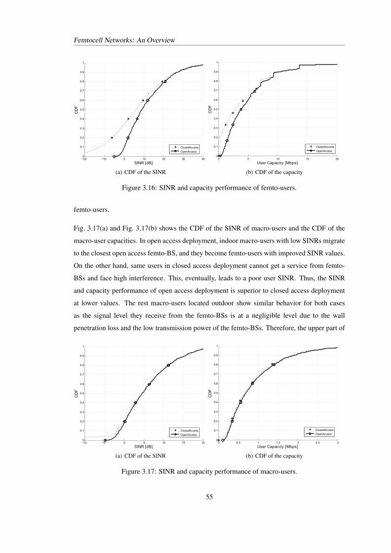
Femtocell Networks: An Overview
−20 −10 0 10 20 30 400
0.1
0.2
0.3
0.4
0.5
0.6
0.7
0.8
0.9
1
SINRn[dB]
CD
F
ClosedAccess
OpenAccess
(a) CDF of the SINR
0 5 10 15 200
0.1
0.2
0.3
0.4
0.5
0.6
0.7
0.8
0.9
1
UserdCapacityd[Mbps]
CD
F
ClosedAccess
OpenAccess
(b) CDF of the capacity
Figure 3.16: SINR and capacity performance of femto-users.
femto-users.
Fig. 3.17(a) and Fig. 3.17(b) shows the CDF of the SINR of macro-users and the CDF of the
macro-user capacities. In open access deployment, indoor macro-users with low SINRs migrate
to the closest open access femto-BS, and they become femto-users with improved SINR values.
On the other hand, same users in closed access deployment cannot get a service from femto-
BSs and face high interference. This, eventually, leads to a poor user SINR. Thus, the SINR
and capacity performance of open access deployment is superior to closed access deployment
at lower values. The rest macro-users located outdoor show similar behavior for both cases
as the signal level they receive from the femto-BSs is at a negligible level due to the wall
penetration loss and the low transmission power of the femto-BSs. Therefore, the upper part of
−10 −5 0 5 10 15 200
0.1
0.2
0.3
0.4
0.5
0.6
0.7
0.8
0.9
1
SINRn[dB]
CD
F
ClosedAccess
OpenAccess
(a) CDF of the SINR
0 0.5 1 1.5 2 2.5 30
0.1
0.2
0.3
0.4
0.5
0.6
0.7
0.8
0.9
1
UserdCapacityd[Mbps]
CD
F
ClosedAccess
OpenAccess
(b) CDF of the capacity
Figure 3.17: SINR and capacity performance of macro-users.
55
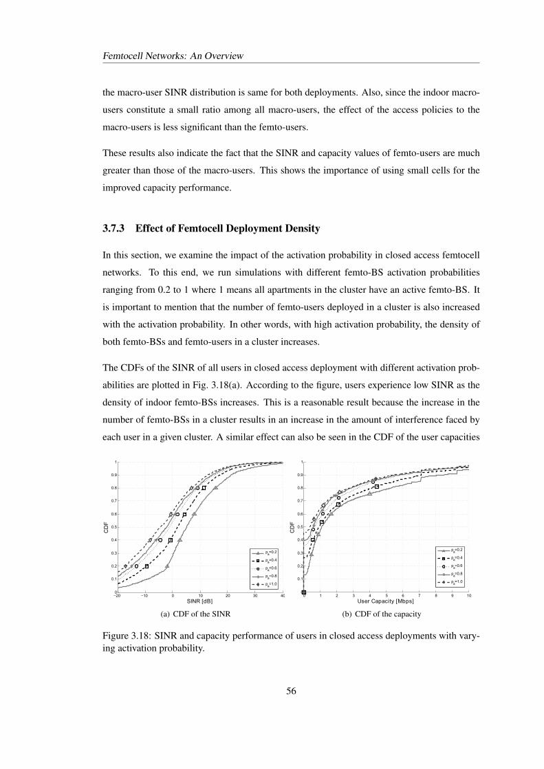
Femtocell Networks: An Overview
the macro-user SINR distribution is same for both deployments. Also, since the indoor macro-
users constitute a small ratio among all macro-users, the effect of the access policies to the
macro-users is less significant than the femto-users.
These results also indicate the fact that the SINR and capacity values of femto-users are much
greater than those of the macro-users. This shows the importance of using small cells for the
improved capacity performance.
3.7.3 Effect of Femtocell Deployment Density
In this section, we examine the impact of the activation probability in closed access femtocell
networks. To this end, we run simulations with different femto-BS activation probabilities
ranging from 0.2 to 1 where 1 means all apartments in the cluster have an active femto-BS. It
is important to mention that the number of femto-users deployed in a cluster is also increased
with the activation probability. In other words, with high activation probability, the density of
both femto-BSs and femto-users in a cluster increases.
The CDFs of the SINR of all users in closed access deployment with different activation prob-
abilities are plotted in Fig. 3.18(a). According to the figure, users experience low SINR as the
density of indoor femto-BSs increases. This is a reasonable result because the increase in the
number of femto-BSs in a cluster results in an increase in the amount of interference faced by
each user in a given cluster. A similar effect can also be seen in the CDF of the user capacities
−20 −10 0 10 20 30 400
0.1
0.2
0.3
0.4
0.5
0.6
0.7
0.8
0.9
1
SINR [dB]
CD
F
pa=0.2
pa=0.4
pa=0.6
pa=0.8
pa=1.0
(a) CDF of the SINR
0 1 2 3 4 5 6 7 8 9 100
0.1
0.2
0.3
0.4
0.5
0.6
0.7
0.8
0.9
1
User Capacity [Mbps]
CD
F
pa=0.2
pa=0.4
pa=0.6
pa=0.8
pa=1.0
(b) CDF of the capacity
Figure 3.18: SINR and capacity performance of users in closed access deployments with vary-ing activation probability.
56
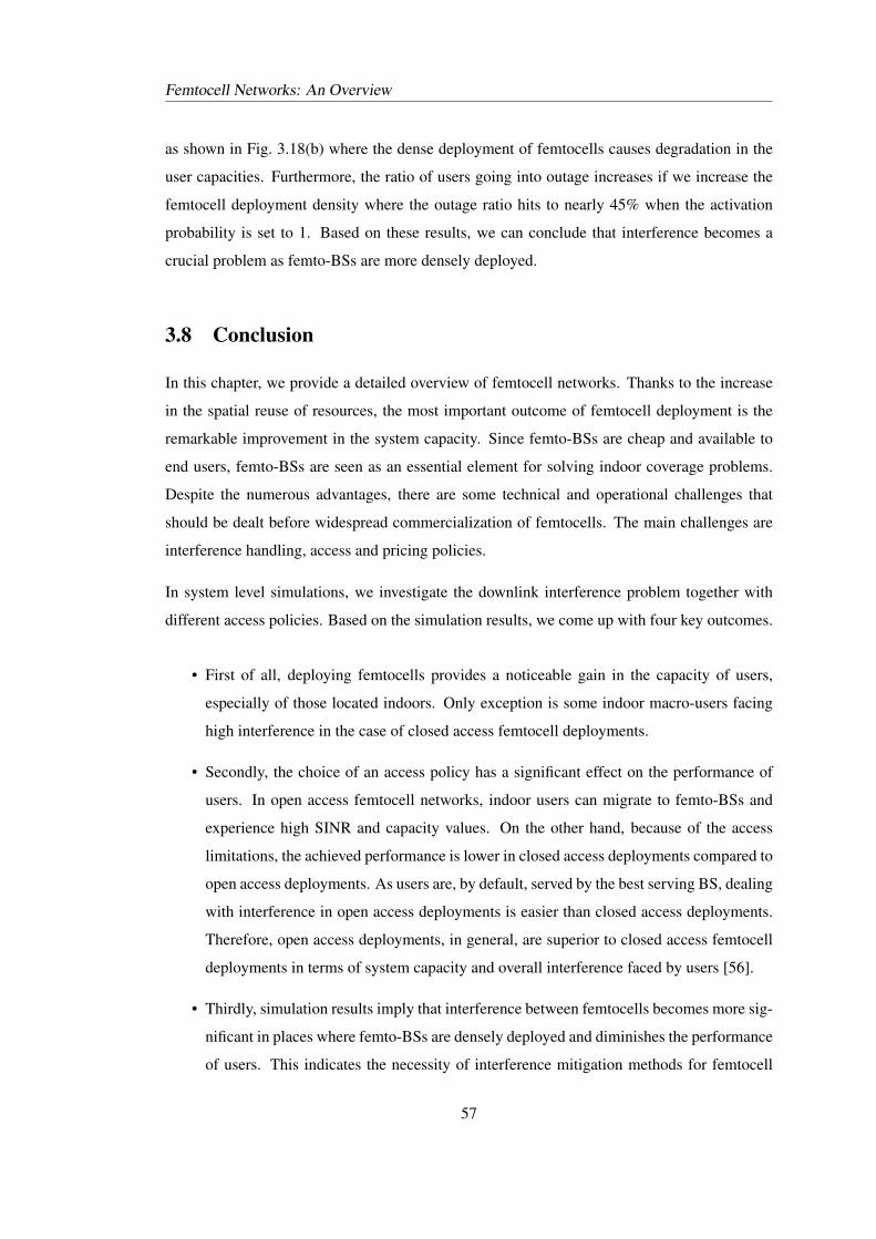
Femtocell Networks: An Overview
as shown in Fig. 3.18(b) where the dense deployment of femtocells causes degradation in the
user capacities. Furthermore, the ratio of users going into outage increases if we increase the
femtocell deployment density where the outage ratio hits to nearly 45% when the activation
probability is set to 1. Based on these results, we can conclude that interference becomes a
crucial problem as femto-BSs are more densely deployed.
3.8 Conclusion
In this chapter, we provide a detailed overview of femtocell networks. Thanks to the increase
in the spatial reuse of resources, the most important outcome of femtocell deployment is the
remarkable improvement in the system capacity. Since femto-BSs are cheap and available to
end users, femto-BSs are seen as an essential element for solving indoor coverage problems.
Despite the numerous advantages, there are some technical and operational challenges that
should be dealt before widespread commercialization of femtocells. The main challenges are
interference handling, access and pricing policies.
In system level simulations, we investigate the downlink interference problem together with
different access policies. Based on the simulation results, we come up with four key outcomes.
• First of all, deploying femtocells provides a noticeable gain in the capacity of users,
especially of those located indoors. Only exception is some indoor macro-users facing
high interference in the case of closed access femtocell deployments.
• Secondly, the choice of an access policy has a significant effect on the performance of
users. In open access femtocell networks, indoor users can migrate to femto-BSs and
experience high SINR and capacity values. On the other hand, because of the access
limitations, the achieved performance is lower in closed access deployments compared to
open access deployments. As users are, by default, served by the best serving BS, dealing
with interference in open access deployments is easier than closed access deployments.
Therefore, open access deployments, in general, are superior to closed access femtocell
deployments in terms of system capacity and overall interference faced by users [56].
• Thirdly, simulation results imply that interference between femtocells becomes more sig-
nificant in places where femto-BSs are densely deployed and diminishes the performance
of users. This indicates the necessity of interference mitigation methods for femtocell
57
Femtocell Networks: An Overview
networks.
• Lastly, the majority of macro-users that are located outside are not affected by the in-
terference from indoor femto-BSs due to the low femto-BS transmit power and the wall
penetration loss.
Based on the outcomes of this chapter, we mainly focus on mitigating the interference in closed
access deployments, which needs a more novel approach, in the following chapters. Since the
interference problems in closed access deployments are more complicated than in open access
deployments, the method that works out in the first would work out in the latter as well. Ad-
ditionally, since the interference between femtocells is more challenging than the interference
between the macrocell and femtocell, we give our priority to mitigate the interference between
femtocells.
58
Chapter 4Interference in Femtocell Networks
4.1 Introduction
In Chapter 3, it is shown that the use of femto-base stations (BSs) over a macrocell network
boosts the system capacity; however, random deployment of femto-BSs causes high inter-
ference to users especially to those located at the intersection of coverage areas of two or
more cells. Downlink interference resulting from femtocell deployments is classified into three
groups that are interference from macrocell to femtocell, from femtocell to macrocell and be-
tween femtocells [26]. Because of the wall penetration loss, the strength of interference from
macro-BS to indoor femto-user and from femto-BS to outdoor macro-user are insignificant in
most situations [57]. The only exception is due to the deployment of closed-access femtocells
where non-subscribed users cannot connect to a closed-access femto-BSs even though they
get the strongest signal from it, and they face severe interference from the femto-BS. On the
other hand, interference between femtocells becomes a crucial problem especially at densely
deployed networks as femto-BSs are deployed in an unplanned manner.
Unlike macrocell networks, operators cannot make an a priori frequency and location planning
for femtocell networks. Thus, interference management at femtocell networks is more challeng-
ing than macrocell networks and requires particular attention. There are two main challenges
to handle interference at femtocell networks. Firstly, as femto-BSs have a dynamic interference
environment where the status and location of femto-BSs can change at any time, interference
management algorithms should be updated during the operation of femto-BSs according to
59
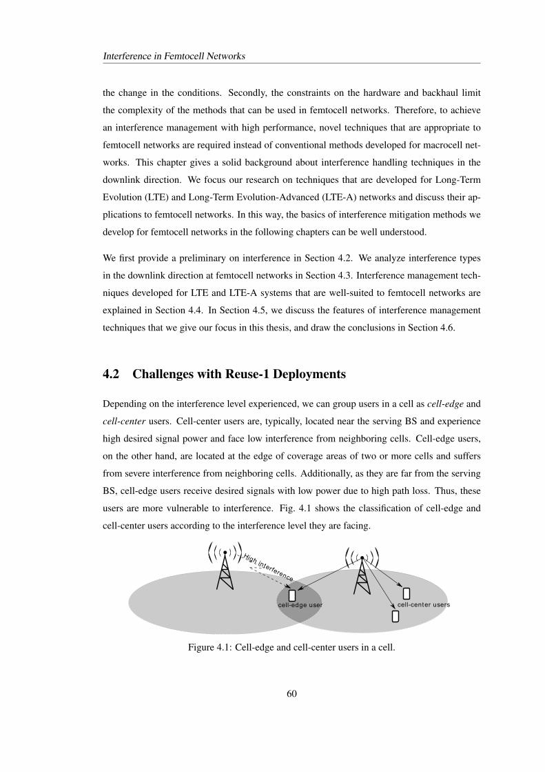
Interference in Femtocell Networks
the change in the conditions. Secondly, the constraints on the hardware and backhaul limit
the complexity of the methods that can be used in femtocell networks. Therefore, to achieve
an interference management with high performance, novel techniques that are appropriate to
femtocell networks are required instead of conventional methods developed for macrocell net-
works. This chapter gives a solid background about interference handling techniques in the
downlink direction. We focus our research on techniques that are developed for Long-Term
Evolution (LTE) and Long-Term Evolution-Advanced (LTE-A) networks and discuss their ap-
plications to femtocell networks. In this way, the basics of interference mitigation methods we
develop for femtocell networks in the following chapters can be well understood.
We first provide a preliminary on interference in Section 4.2. We analyze interference types
in the downlink direction at femtocell networks in Section 4.3. Interference management tech-
niques developed for LTE and LTE-A systems that are well-suited to femtocell networks are
explained in Section 4.4. In Section 4.5, we discuss the features of interference management
techniques that we give our focus in this thesis, and draw the conclusions in Section 4.6.
4.2 Challenges with Reuse-1 Deployments
Depending on the interference level experienced, we can group users in a cell as cell-edge and
cell-center users. Cell-center users are, typically, located near the serving BS and experience
high desired signal power and face low interference from neighboring cells. Cell-edge users,
on the other hand, are located at the edge of coverage areas of two or more cells and suffers
from severe interference from neighboring cells. Additionally, as they are far from the serving
BS, cell-edge users receive desired signals with low power due to high path loss. Thus, these
users are more vulnerable to interference. Fig. 4.1 shows the classification of cell-edge and
cell-center users according to the interference level they are facing.
High interference
cell-center userscell-edge user
Figure 4.1: Cell-edge and cell-center users in a cell.
60
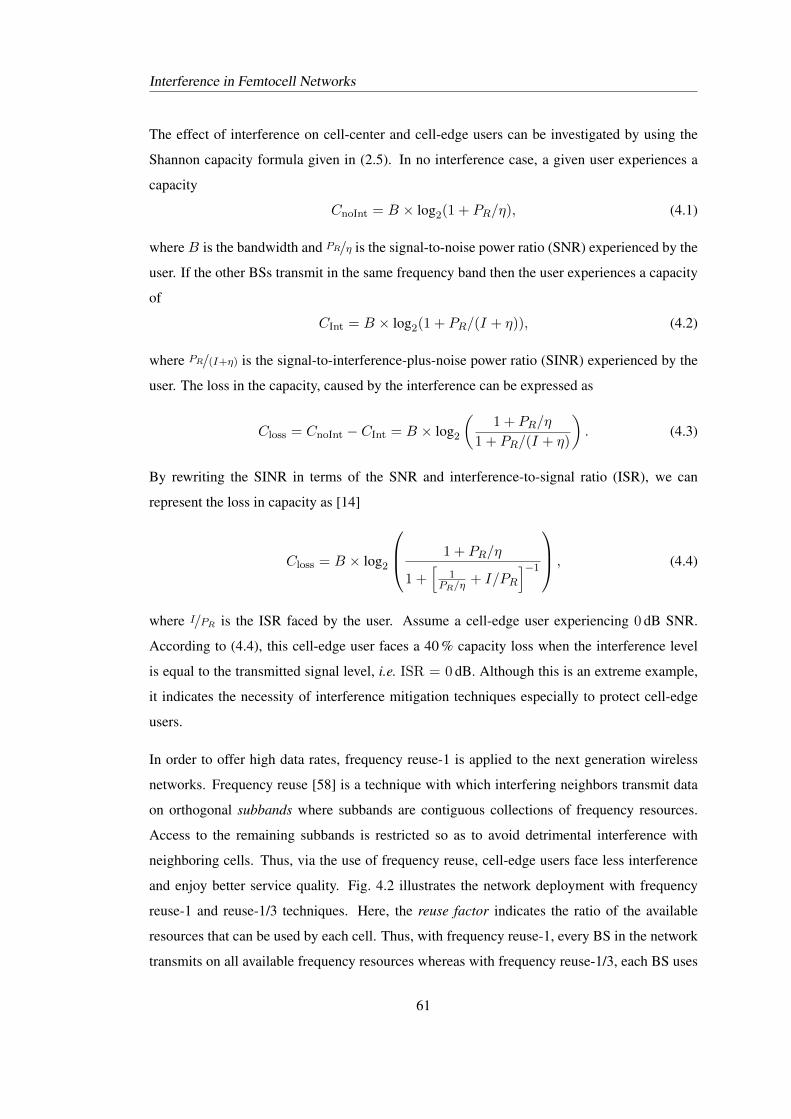
Interference in Femtocell Networks
The effect of interference on cell-center and cell-edge users can be investigated by using the
Shannon capacity formula given in (2.5). In no interference case, a given user experiences a
capacity
CnoInt = B × log2(1 + PR/η), (4.1)
where B is the bandwidth and PR/η is the signal-to-noise power ratio (SNR) experienced by the
user. If the other BSs transmit in the same frequency band then the user experiences a capacity
of
CInt = B × log2(1 + PR/(I + η)), (4.2)
where PR/(I+η) is the signal-to-interference-plus-noise power ratio (SINR) experienced by the
user. The loss in the capacity, caused by the interference can be expressed as
Closs = CnoInt − CInt = B × log2
(1 + PR/η
1 + PR/(I + η)
). (4.3)
By rewriting the SINR in terms of the SNR and interference-to-signal ratio (ISR), we can
represent the loss in capacity as [14]
Closs = B × log2
1 + PR/η
1 +[
1PR/η
+ I/PR
]−1
, (4.4)
where I/PR is the ISR faced by the user. Assume a cell-edge user experiencing 0 dB SNR.
According to (4.4), this cell-edge user faces a 40 % capacity loss when the interference level
is equal to the transmitted signal level, i.e. ISR = 0 dB. Although this is an extreme example,
it indicates the necessity of interference mitigation techniques especially to protect cell-edge
users.
In order to offer high data rates, frequency reuse-1 is applied to the next generation wireless
networks. Frequency reuse [58] is a technique with which interfering neighbors transmit data
on orthogonal subbands where subbands are contiguous collections of frequency resources.
Access to the remaining subbands is restricted so as to avoid detrimental interference with
neighboring cells. Thus, via the use of frequency reuse, cell-edge users face less interference
and enjoy better service quality. Fig. 4.2 illustrates the network deployment with frequency
reuse-1 and reuse-1/3 techniques. Here, the reuse factor indicates the ratio of the available
resources that can be used by each cell. Thus, with frequency reuse-1, every BS in the network
transmits on all available frequency resources whereas with frequency reuse-1/3, each BS uses
61
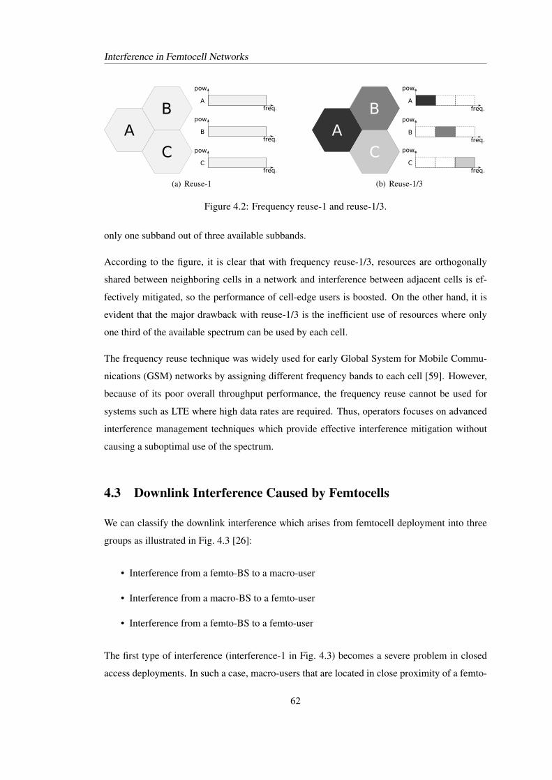
Interference in Femtocell Networks
freq.
pow.
A
freq.
pow.
B
freq.
pow.
C
AB
C
(a) Reuse-1
freq.
pow.
A
freq.
pow.
B
freq.
pow.
C
AB
C
(b) Reuse-1/3
Figure 4.2: Frequency reuse-1 and reuse-1/3.
only one subband out of three available subbands.
According to the figure, it is clear that with frequency reuse-1/3, resources are orthogonally
shared between neighboring cells in a network and interference between adjacent cells is ef-
fectively mitigated, so the performance of cell-edge users is boosted. On the other hand, it is
evident that the major drawback with reuse-1/3 is the inefficient use of resources where only
one third of the available spectrum can be used by each cell.
The frequency reuse technique was widely used for early Global System for Mobile Commu-
nications (GSM) networks by assigning different frequency bands to each cell [59]. However,
because of its poor overall throughput performance, the frequency reuse cannot be used for
systems such as LTE where high data rates are required. Thus, operators focuses on advanced
interference management techniques which provide effective interference mitigation without
causing a suboptimal use of the spectrum.
4.3 Downlink Interference Caused by Femtocells
We can classify the downlink interference which arises from femtocell deployment into three
groups as illustrated in Fig. 4.3 [26]:
• Interference from a femto-BS to a macro-user
• Interference from a macro-BS to a femto-user
• Interference from a femto-BS to a femto-user
The first type of interference (interference-1 in Fig. 4.3) becomes a severe problem in closed
access deployments. In such a case, macro-users that are located in close proximity of a femto-
62
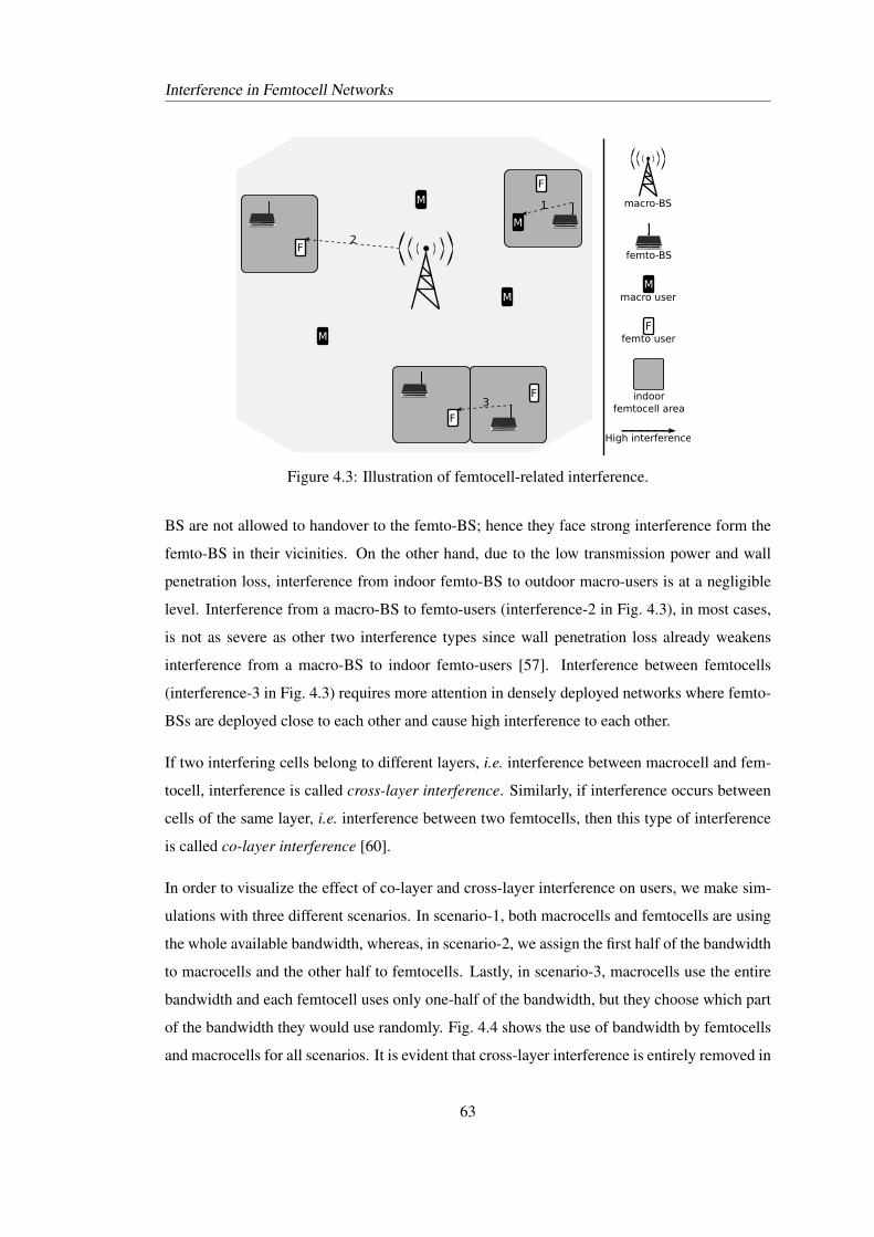
Interference in Femtocell Networks
macro-BS
femto-BS
Mmacro user
Ffemto user
indoor femtocell area
High interference
F
F
F
M
M
M
M
F
1
3
2
Figure 4.3: Illustration of femtocell-related interference.
BS are not allowed to handover to the femto-BS; hence they face strong interference form the
femto-BS in their vicinities. On the other hand, due to the low transmission power and wall
penetration loss, interference from indoor femto-BS to outdoor macro-users is at a negligible
level. Interference from a macro-BS to femto-users (interference-2 in Fig. 4.3), in most cases,
is not as severe as other two interference types since wall penetration loss already weakens
interference from a macro-BS to indoor femto-users [57]. Interference between femtocells
(interference-3 in Fig. 4.3) requires more attention in densely deployed networks where femto-
BSs are deployed close to each other and cause high interference to each other.
If two interfering cells belong to different layers, i.e. interference between macrocell and fem-
tocell, interference is called cross-layer interference. Similarly, if interference occurs between
cells of the same layer, i.e. interference between two femtocells, then this type of interference
is called co-layer interference [60].
In order to visualize the effect of co-layer and cross-layer interference on users, we make sim-
ulations with three different scenarios. In scenario-1, both macrocells and femtocells are using
the whole available bandwidth, whereas, in scenario-2, we assign the first half of the bandwidth
to macrocells and the other half to femtocells. Lastly, in scenario-3, macrocells use the entire
bandwidth and each femtocell uses only one-half of the bandwidth, but they choose which part
of the bandwidth they would use randomly. Fig. 4.4 shows the use of bandwidth by femtocells
and macrocells for all scenarios. It is evident that cross-layer interference is entirely removed in
63
Interference in Femtocell Networks
scenario-2 as different frequency bands are assigned to femtocells and macrocells. The draw-
back of scenario-2 is the inefficient resource utilization due to the restriction on the use of the
spectrum by BSs. Furthermore, the co-layer interference between femtocells still remains un-
solved. In scenario-3, we use a straightforward interference mitigation technique to decrease
interference between femto-BSs by allowing femto-BSs to operate on two different frequency
bands. This can be seen as a reuse-1/2 technique where resources are assigned by femto-BSs
randomly.
freq.
pow.
macro-BS
femto-BS
freq.
pow.
freq.
pow.
Scenario-1
freq.
pow.
freq.
pow.
Scenario-2
freq.
pow.
Scenario-3
freq.
pow. OR
Figure 4.4: Bandwidth assignments of macrocells and femtocells for three different scenarios.
For simulations, we use a simulation setup based on the 3rd Generation Partnership Project
(3GPP) specifications. The simulation setup is explained in Chapter 3 in a detailed way. The
Monte Carlo simulation consists of snapshots each of which has a time duration of 1 ms (i.e. one
subframe). Also, we assume that positions and shadowing values of users do not change during
the snapshot. Each macrocell has one 5×5 grid structure where the 5×5 grid indicates 25 reg-
ularly arranged square-shaped apartments [49]. Only closed access femtocells are considered
where femto-BSs are deployed in an apartment with an activation probability of pa=0.2. If
an apartment contains an active femto-BS, it serves minimum 1, maximum 4 femto-users that
are randomly distributed within the confines of the same apartment. On the other hand, each
macrocell serves 10 macro-users on average. We assume that every BS assigns all available
resource blocks to its served users. All parameters that are used for the simulation are listed in
Table 3.3.
In order to plot the cumulative distribution function (CDF) of the SINR of users, at the end of
each snapshot, we use the average SINR experienced by users. The average SINR of user u is
64
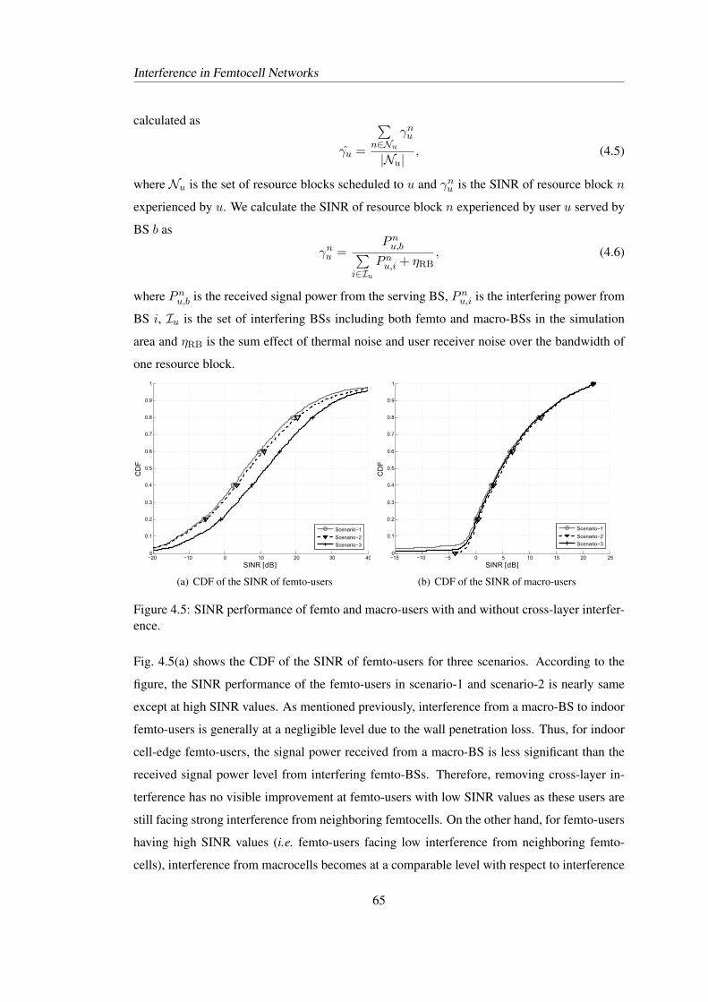
Interference in Femtocell Networks
calculated as
γu =
∑n∈Nu
γnu
|Nu|, (4.5)
where Nu is the set of resource blocks scheduled to u and γnu is the SINR of resource block n
experienced by u. We calculate the SINR of resource block n experienced by user u served by
BS b as
γnu =Pnu,b∑
i∈IuPnu,i + ηRB
, (4.6)
where Pnu,b is the received signal power from the serving BS, Pnu,i is the interfering power from
BS i, Iu is the set of interfering BSs including both femto and macro-BSs in the simulation
area and ηRB is the sum effect of thermal noise and user receiver noise over the bandwidth of
one resource block.
−20 −10 0 10 20 30 400
0.1
0.2
0.3
0.4
0.5
0.6
0.7
0.8
0.9
1
SINR [dB]
CD
F
Scenario−1
Scenario−2
Scenario−3
(a) CDF of the SINR of femto-users
−15 −10 −5 0 5 10 15 20 250
0.1
0.2
0.3
0.4
0.5
0.6
0.7
0.8
0.9
1
SINR [dB]
CD
F
Scenario−1
Scenario−2
Scenario−3
(b) CDF of the SINR of macro-users
Figure 4.5: SINR performance of femto and macro-users with and without cross-layer interfer-ence.
Fig. 4.5(a) shows the CDF of the SINR of femto-users for three scenarios. According to the
figure, the SINR performance of the femto-users in scenario-1 and scenario-2 is nearly same
except at high SINR values. As mentioned previously, interference from a macro-BS to indoor
femto-users is generally at a negligible level due to the wall penetration loss. Thus, for indoor
cell-edge femto-users, the signal power received from a macro-BS is less significant than the
received signal power level from interfering femto-BSs. Therefore, removing cross-layer in-
terference has no visible improvement at femto-users with low SINR values as these users are
still facing strong interference from neighboring femtocells. On the other hand, for femto-users
having high SINR values (i.e. femto-users facing low interference from neighboring femto-
cells), interference from macrocells becomes at a comparable level with respect to interference
65
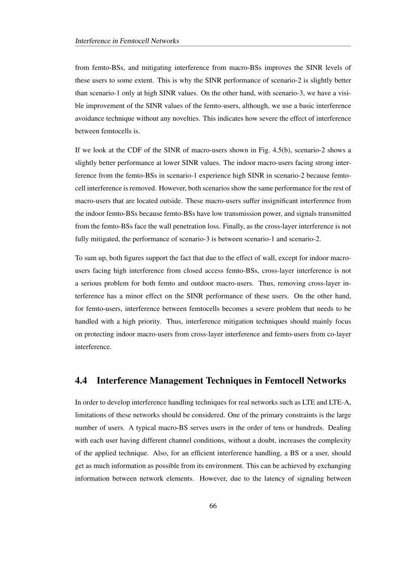
Interference in Femtocell Networks
from femto-BSs, and mitigating interference from macro-BSs improves the SINR levels of
these users to some extent. This is why the SINR performance of scenario-2 is slightly better
than scenario-1 only at high SINR values. On the other hand, with scenario-3, we have a visi-
ble improvement of the SINR values of the femto-users, although, we use a basic interference
avoidance technique without any novelties. This indicates how severe the effect of interference
between femtocells is.
If we look at the CDF of the SINR of macro-users shown in Fig. 4.5(b), scenario-2 shows a
slightly better performance at lower SINR values. The indoor macro-users facing strong inter-
ference from the femto-BSs in scenario-1 experience high SINR in scenario-2 because femto-
cell interference is removed. However, both scenarios show the same performance for the rest of
macro-users that are located outside. These macro-users suffer insignificant interference from
the indoor femto-BSs because femto-BSs have low transmission power, and signals transmitted
from the femto-BSs face the wall penetration loss. Finally, as the cross-layer interference is not
fully mitigated, the performance of scenario-3 is between scenario-1 and scenario-2.
To sum up, both figures support the fact that due to the effect of wall, except for indoor macro-
users facing high interference from closed access femto-BSs, cross-layer interference is not
a serious problem for both femto and outdoor macro-users. Thus, removing cross-layer in-
terference has a minor effect on the SINR performance of these users. On the other hand,
for femto-users, interference between femtocells becomes a severe problem that needs to be
handled with a high priority. Thus, interference mitigation techniques should mainly focus
on protecting indoor macro-users from cross-layer interference and femto-users from co-layer
interference.
4.4 Interference Management Techniques in Femtocell Networks
In order to develop interference handling techniques for real networks such as LTE and LTE-A,
limitations of these networks should be considered. One of the primary constraints is the large
number of users. A typical macro-BS serves users in the order of tens or hundreds. Dealing
with each user having different channel conditions, without a doubt, increases the complexity
of the applied technique. Also, for an efficient interference handling, a BS or a user, should
get as much information as possible from its environment. This can be achieved by exchanging
information between network elements. However, due to the latency of signaling between
66
Interference in Femtocell Networks
network elements, it is not possible to respond to changes in channel conditions immediately.
Apart from multi-user deployments and delay in signaling, there are other limitations coming
with practical implementations such as errors in channel estimation, restrictions on the amount
and type of information signals to be transmitted.
Different from macrocell networks, the major challenge of interference handling in femtocell
networks arises from the access policies. Due to the restricted access policies, a user may not
handover to the nearest femtocell with closed access if the user does not belong to the sub-
scriber group of the femtocell. Thus, the user faces strong interference. Additionally, femto-
BSs have a simpler hardware than macro-BSs as they are planned to be low-cost devices having
low-complexity receivers for end-users [6]. Furthermore, the backhaul connection provided to
femtocell networks is mostly based on the digital subscriber line (DSL) technology having lim-
ited capacity and high delay with respect to the backhaul connection between macro-BSs [61].
Therefore, the methods requiring a high amount of information exchange between network el-
ements or complex antenna and receiver hardware are not appropriate for femtocell networks.
Last but not least, because of their uncoordinated nature; femto-BSs are deployed in an ad
hoc manner so that their position can be changed, or they can be switched on or off at any
time. Thus, elaborate network planning and resource optimization do not work efficiently at
femtocell networks.
In order to deal with such challenges, users should be capable of sensing the environment and
inform their serving cells about the potential interferers and the channel conditions. Further-
more, BSs should be able to communicate and collaborate with the potential interfering BSs
to achieve an effective interference management. In order to overcome such challenges, LTE
(3GPP Release-8 and Release-9) offers dynamic inter-BS coordination known as inter-cell in-
terference coordination (ICIC). The aim of ICIC is to suppress interference between cells by
managing the use of resources between BSs. This is mainly done by resource partitioning
methods by sharing the frequency or time resources among BSs in a coordinated way [62]. In
addition to the resource partitioning, power control over the transmitted resources is another
ICIC method used for managing interference. It is also possible to apply frequency sharing and
power control together to get better performance.
In 3GPP, two cases of ICIC are supported by LTE; static and semi-static ICIC [63]. In static
ICIC, cells update the resource configuration on a time scale corresponding to days. There-
fore, the communication between cells is limited. In semi-static ICIC, on the other hand, cells
67
Interference in Femtocell Networks
reconfigure their resource usage on a time scale corresponding to seconds or longer; thus, com-
munication between cells becomes crucial.
In addition to ICIC defined in Release-8 and Release-9, 3GPP also defines enhanced inter-cell
interference coordination (eICIC) with LTE-A (more precisely starting from Release-10). The
main focus of eICIC is to protect control channels in heterogeneous networks (Het-Nets).
4.4.1 Inter-cell Interference Coordination
In LTE Release-8 and Release-9, frequency domain based ICIC tools are supported especially
for improving the data transmission [14]. For this purpose, three messages signaled between
BSs are defined. These messages are relative narrowband transmit power (RNTP) that is used
for the downlink scheduling, and high interference indicator (HII) and overload indicator (OI)
which are used for the uplink interference coordination [64]. With these messages, BSs in-
form each other about which uplink or downlink resources are currently used. However, in
order to allow freedom and flexibility to BSs for the scheduling of resources, the reaction of a
BS upon receiving of these ICIC-related messages from a neighboring BS is not standardized
(i.e. depends on the scheduling policy of an operator) [14].
ICIC messages that convey information about the scheduling strategy of BSs are transmitted
between BSs by using the X2 interface. X2 is a logical interface and used for connecting BSs
through which BSs can exchange information related with handover, load or interference [40].
The X2 interface between femto-BSs was not defined in Release-8 and Release-9. However,
starting from Release-10, this interface is also supported between femto-BSs in order to support
the mobility [1]. Due to the latency over the X2 interface (it is typically with the order of tens
of milli-seconds [65]), it is expected that the update rate of these messages is less frequent than
the scheduling period of the resources which is 1 ms [66].
Table 4.1 gives an overview of the mentioned ICIC messages [14, 67–69] and the detailed
explanation of these messages is given in the sequel.
4.4.1.1 Relative Narrowband Transmit Power (RNTP)
The RNTP provides an indication of downlink power restriction per resource block in a cell.
It is reported as a bitmap where each position in the bitmap corresponds to one resource block
68
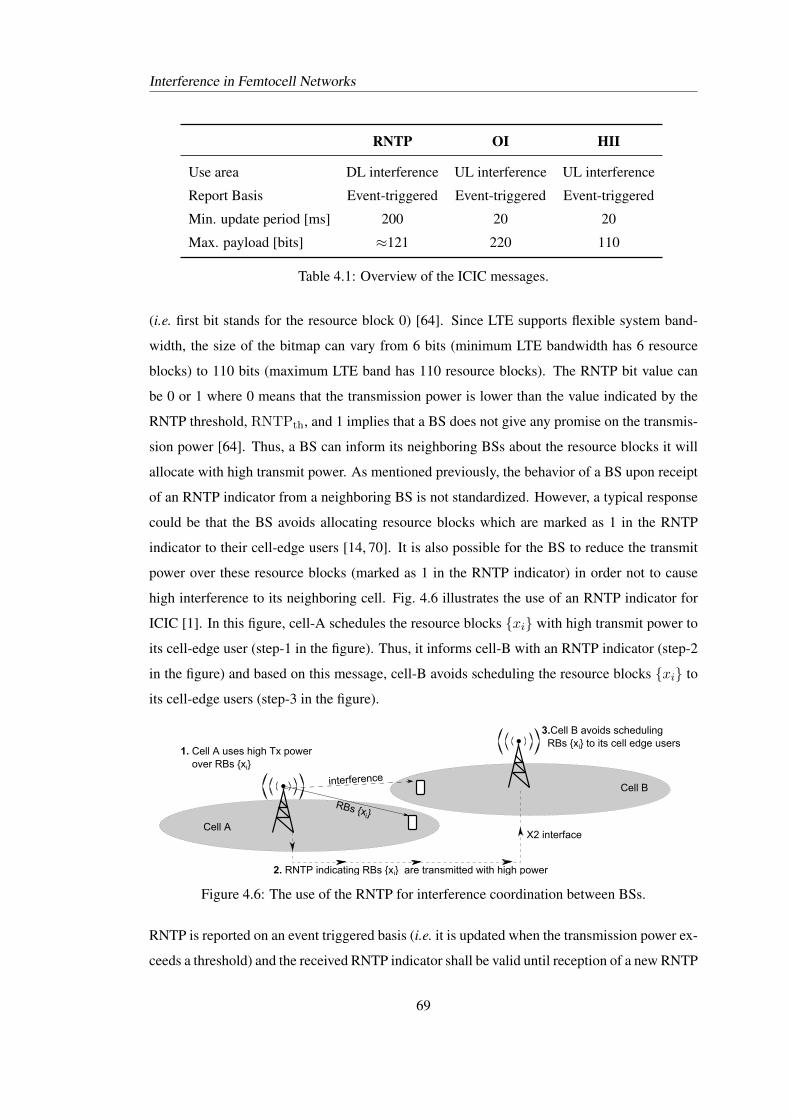
Interference in Femtocell Networks
RNTP OI HII
Use area DL interference UL interference UL interference
Report Basis Event-triggered Event-triggered Event-triggered
Min. update period [ms] 200 20 20
Max. payload [bits] ≈121 220 110
Table 4.1: Overview of the ICIC messages.
(i.e. first bit stands for the resource block 0) [64]. Since LTE supports flexible system band-
width, the size of the bitmap can vary from 6 bits (minimum LTE bandwidth has 6 resource
blocks) to 110 bits (maximum LTE band has 110 resource blocks). The RNTP bit value can
be 0 or 1 where 0 means that the transmission power is lower than the value indicated by the
RNTP threshold, RNTPth, and 1 implies that a BS does not give any promise on the transmis-
sion power [64]. Thus, a BS can inform its neighboring BSs about the resource blocks it will
allocate with high transmit power. As mentioned previously, the behavior of a BS upon receipt
of an RNTP indicator from a neighboring BS is not standardized. However, a typical response
could be that the BS avoids allocating resource blocks which are marked as 1 in the RNTP
indicator to their cell-edge users [14, 70]. It is also possible for the BS to reduce the transmit
power over these resource blocks (marked as 1 in the RNTP indicator) in order not to cause
high interference to its neighboring cell. Fig. 4.6 illustrates the use of an RNTP indicator for
ICIC [1]. In this figure, cell-A schedules the resource blocks {xi} with high transmit power to
its cell-edge user (step-1 in the figure). Thus, it informs cell-B with an RNTP indicator (step-2
in the figure) and based on this message, cell-B avoids scheduling the resource blocks {xi} to
its cell-edge users (step-3 in the figure).
X2minterface
1.mCellmAmusesmhighmTxmpowermmmmovermRBsm{xi}mm
CellmA
CellmB
2.mRNTPmindicatingmRBsm{xi}mmaremtransmittedmwithmhighmpower
3.CellmBmavoidsmschedulingmmmRBsm{xi}mtomitsmcellmedgemusersm
RBsm{xi}
interference
Figure 4.6: The use of the RNTP for interference coordination between BSs.
RNTP is reported on an event triggered basis (i.e. it is updated when the transmission power ex-
ceeds a threshold) and the received RNTP indicator shall be valid until reception of a new RNTP
69
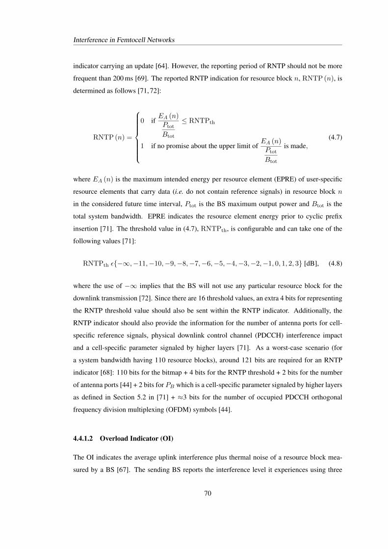
Interference in Femtocell Networks
indicator carrying an update [64]. However, the reporting period of RNTP should not be more
frequent than 200 ms [69]. The reported RNTP indication for resource block n, RNTP (n), is
determined as follows [71, 72]:
RNTP (n) =
0 ifEA (n)Ptot
Btot
≤ RNTPth
1 if no promise about the upper limit ofEA (n)Ptot
Btot
is made,(4.7)
where EA (n) is the maximum intended energy per resource element (EPRE) of user-specific
resource elements that carry data (i.e. do not contain reference signals) in resource block n
in the considered future time interval, Ptot is the BS maximum output power and Btot is the
total system bandwidth. EPRE indicates the resource element energy prior to cyclic prefix
insertion [71]. The threshold value in (4.7), RNTPth, is configurable and can take one of the
following values [71]:
RNTPth ε{−∞,−11,−10,−9,−8,−7,−6,−5,−4,−3,−2,−1, 0, 1, 2, 3} [dB], (4.8)
where the use of −∞ implies that the BS will not use any particular resource block for the
downlink transmission [72]. Since there are 16 threshold values, an extra 4 bits for representing
the RNTP threshold value should also be sent within the RNTP indicator. Additionally, the
RNTP indicator should also provide the information for the number of antenna ports for cell-
specific reference signals, physical downlink control channel (PDCCH) interference impact
and a cell-specific parameter signaled by higher layers [71]. As a worst-case scenario (for
a system bandwidth having 110 resource blocks), around 121 bits are required for an RNTP
indicator [68]: 110 bits for the bitmap + 4 bits for the RNTP threshold + 2 bits for the number
of antenna ports [44] + 2 bits for PB which is a cell-specific parameter signaled by higher layers
as defined in Section 5.2 in [71] + ≈3 bits for the number of occupied PDCCH orthogonal
frequency division multiplexing (OFDM) symbols [44].
4.4.1.2 Overload Indicator (OI)
The OI indicates the average uplink interference plus thermal noise of a resource block mea-
sured by a BS [67]. The sending BS reports the interference level it experiences using three
70
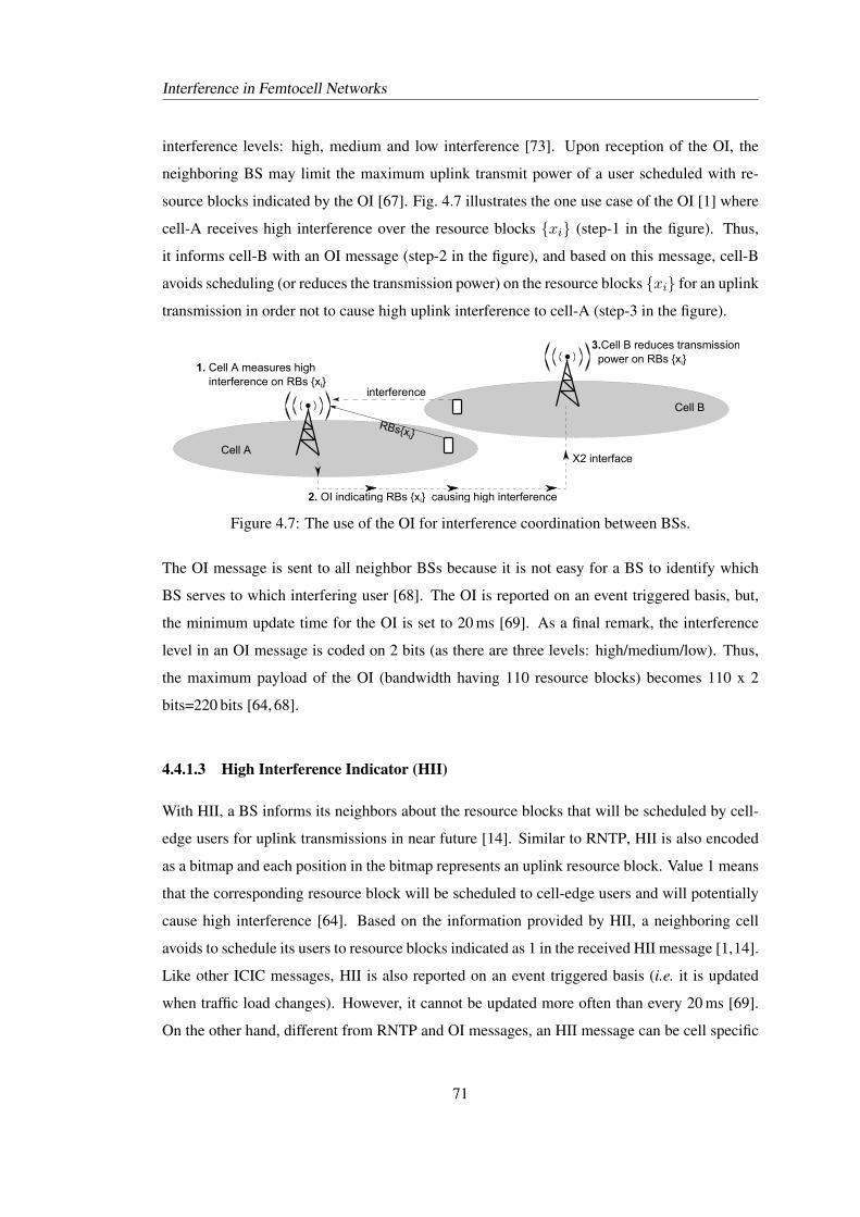
Interference in Femtocell Networks
interference levels: high, medium and low interference [73]. Upon reception of the OI, the
neighboring BS may limit the maximum uplink transmit power of a user scheduled with re-
source blocks indicated by the OI [67]. Fig. 4.7 illustrates the one use case of the OI [1] where
cell-A receives high interference over the resource blocks {xi} (step-1 in the figure). Thus,
it informs cell-B with an OI message (step-2 in the figure), and based on this message, cell-B
avoids scheduling (or reduces the transmission power) on the resource blocks {xi} for an uplink
transmission in order not to cause high uplink interference to cell-A (step-3 in the figure).
X2 interface
1. Cell A measures high interference on RBs {xi}
Cell A
Cell B
2. OI indicating RBs {xi} causing high interference
3.Cell B reduces transmission power on RBs {xi}
RBs{xi}
interference
Figure 4.7: The use of the OI for interference coordination between BSs.
The OI message is sent to all neighbor BSs because it is not easy for a BS to identify which
BS serves to which interfering user [68]. The OI is reported on an event triggered basis, but,
the minimum update time for the OI is set to 20 ms [69]. As a final remark, the interference
level in an OI message is coded on 2 bits (as there are three levels: high/medium/low). Thus,
the maximum payload of the OI (bandwidth having 110 resource blocks) becomes 110 x 2
bits=220 bits [64, 68].
4.4.1.3 High Interference Indicator (HII)
With HII, a BS informs its neighbors about the resource blocks that will be scheduled by cell-
edge users for uplink transmissions in near future [14]. Similar to RNTP, HII is also encoded
as a bitmap and each position in the bitmap represents an uplink resource block. Value 1 means
that the corresponding resource block will be scheduled to cell-edge users and will potentially
cause high interference [64]. Based on the information provided by HII, a neighboring cell
avoids to schedule its users to resource blocks indicated as 1 in the received HII message [1,14].
Like other ICIC messages, HII is also reported on an event triggered basis (i.e. it is updated
when traffic load changes). However, it cannot be updated more often than every 20 ms [69].
On the other hand, different from RNTP and OI messages, an HII message can be cell specific
71
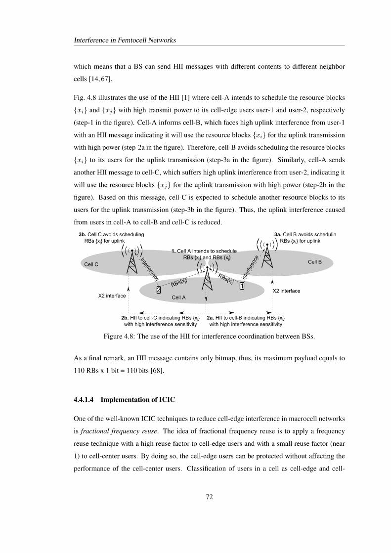
Interference in Femtocell Networks
which means that a BS can send HII messages with different contents to different neighbor
cells [14, 67].
Fig. 4.8 illustrates the use of the HII [1] where cell-A intends to schedule the resource blocks
{xi} and {xj} with high transmit power to its cell-edge users user-1 and user-2, respectively
(step-1 in the figure). Cell-A informs cell-B, which faces high uplink interference from user-1
with an HII message indicating it will use the resource blocks {xi} for the uplink transmission
with high power (step-2a in the figure). Therefore, cell-B avoids scheduling the resource blocks
{xi} to its users for the uplink transmission (step-3a in the figure). Similarly, cell-A sends
another HII message to cell-C, which suffers high uplink interference from user-2, indicating it
will use the resource blocks {xj} for the uplink transmission with high power (step-2b in the
figure). Based on this message, cell-C is expected to schedule another resource blocks to its
users for the uplink transmission (step-3b in the figure). Thus, the uplink interference caused
from users in cell-A to cell-B and cell-C is reduced.
X2yinterface
1.yCellyAyintendsytoyscheduleyyyyyRBsy{xi}yandyRBsy{xj}
CellyA
CellyB
2a.yHIIytoycell-ByindicatingyRBsy{xi}ywithyhighyinterferenceysensitivity
3a.yCellyByavoidsyschedulingyyyyyRBsy{xi}yforyuplinky
inte
rfere
nce
RBs{xi }
RBs{xj}
CellyC
12
interference3b.yCellyCyavoidsyschedulingyyyyyRBsy{xj}yforyuplinky
X2yinterface
2b.yHIIytoycell-CyindicatingyRBsy{xj}ywithyhighyinterferenceysensitivity
Figure 4.8: The use of the HII for interference coordination between BSs.
As a final remark, an HII message contains only bitmap, thus, its maximum payload equals to
110 RBs x 1 bit = 110 bits [68].
4.4.1.4 Implementation of ICIC
One of the well-known ICIC techniques to reduce cell-edge interference in macrocell networks
is fractional frequency reuse. The idea of fractional frequency reuse is to apply a frequency
reuse technique with a high reuse factor to cell-edge users and with a small reuse factor (near
1) to cell-center users. By doing so, the cell-edge users can be protected without affecting the
performance of the cell-center users. Classification of users in a cell as cell-edge and cell-
72
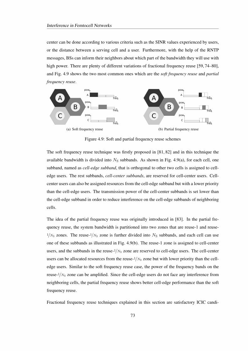
Interference in Femtocell Networks
center can be done according to various criteria such as the SINR values experienced by users,
or the distance between a serving cell and a user. Furthermore, with the help of the RNTP
messages, BSs can inform their neighbors about which part of the bandwidth they will use with
high power. There are plenty of different variations of fractional frequency reuse [59, 74–80],
and Fig. 4.9 shows the two most common ones which are the soft frequency reuse and partial
frequency reuse.
freq.
pow.
A
freq.
pow.
B
freq.
pow.
C
AB
C
(a) Soft frequency reuse
freq.
pow.
A
freq.
pow.
B
freq.
pow.
C
AB
C
(b) Partial frequency reuse
Figure 4.9: Soft and partial frequency reuse schemes
The soft frequency reuse technique was firstly proposed in [81, 82] and in this technique the
available bandwidth is divided into NS subbands. As shown in Fig. 4.9(a), for each cell, one
subband, named as cell-edge subband, that is orthogonal to other two cells is assigned to cell-
edge users. The rest subbands, cell-center subbands, are reserved for cell-center users. Cell-
center users can also be assigned resources from the cell-edge subband but with a lower priority
than the cell-edge users. The transmission power of the cell-center subbands is set lower than
the cell-edge subband in order to reduce interference on the cell-edge subbands of neighboring
cells.
The idea of the partial frequency reuse was originally introduced in [83]. In the partial fre-
quency reuse, the system bandwidth is partitioned into two zones that are reuse-1 and reuse-
1/NS zones. The reuse-1/NS zone is further divided into NS subbands, and each cell can use
one of these subbands as illustrated in Fig. 4.9(b). The reuse-1 zone is assigned to cell-center
users, and the subbands in the reuse-1/NS zone are reserved to cell-edge users. The cell-center
users can be allocated resources from the reuse-1/NS zone but with lower priority than the cell-
edge users. Similar to the soft frequency reuse case, the power of the frequency bands on the
reuse-1/NS zone can be amplified. Since the cell-edge users do not face any interference from
neighboring cells, the partial frequency reuse shows better cell-edge performance than the soft
frequency reuse.
Fractional frequency reuse techniques explained in this section are satisfactory ICIC candi-
73
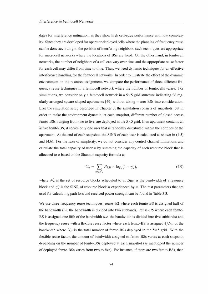
Interference in Femtocell Networks
dates for interference mitigation, as they show high cell-edge performance with low complex-
ity. Since they are developed for operator-deployed cells where the planning of frequency reuse
can be done according to the position of interfering neighbors, such techniques are appropriate
for macrocell networks where the locations of BSs are fixed. On the other hand, in femtocell
networks, the number of neighbors of a cell can vary over time and the appropriate reuse factor
for each cell may differ from time to time. Thus, we need dynamic techniques for an effective
interference handling for the femtocell networks. In order to illustrate the effect of the dynamic
environment on the resource assignment, we compare the performance of three different fre-
quency reuse techniques in a femtocell network where the number of femtocells varies. For
simulations, we consider only a femtocell network in a 5×5 grid structure indicating 25 reg-
ularly arranged square-shaped apartments [49] without taking macro-BSs into consideration.
Like the simulation setup described in Chapter 3; the simulation consists of snapshots, but in
order to make the environment dynamic, at each snapshot, different number of closed-access
femto-BSs, ranging from two to five, are deployed in the 5×5 grid. If an apartment contains an
active femto-BS, it serves only one user that is randomly distributed within the confines of the
apartment. At the end of each snapshot, the SINR of each user is calculated as shown in (4.5)
and (4.6). For the sake of simplicity, we do not consider any control channel limitations and
calculate the total capacity of user u by summing the capacity of each resource block that is
allocated to u based on the Shannon capacity formula as
Cu =∑n∈Nu
BRB × log2(1 + γnu ), (4.9)
where Nu is the set of resource blocks scheduled to u, BRB is the bandwidth of a resource
block and γnu is the SINR of resource block n experienced by u. The rest parameters that are
used for calculating path loss and received power strength can be found in Table 3.3.
We use three frequency reuse techniques; reuse-1/2 where each femto-BS is assigned half of
the bandwidth (i.e. the bandwidth is divided into two subbands), reuse-1/5 where each femto-
BS is assigned one fifth of the bandwidth (i.e. the bandwidth is divided into five subbands) and
the frequency reuse with a flexible reuse factor where each femto-BS is assigned 1/NF of the
bandwidth where NF is the total number of femto-BSs deployed in the 5×5 grid. With the
flexible reuse factor, the amount of bandwidth assigned to femto-BSs varies at each snapshot
depending on the number of femto-BSs deployed at each snapshot (as mentioned the number
of deployed femto-BSs varies from two to five). For instance, if there are two femto-BSs, then
74
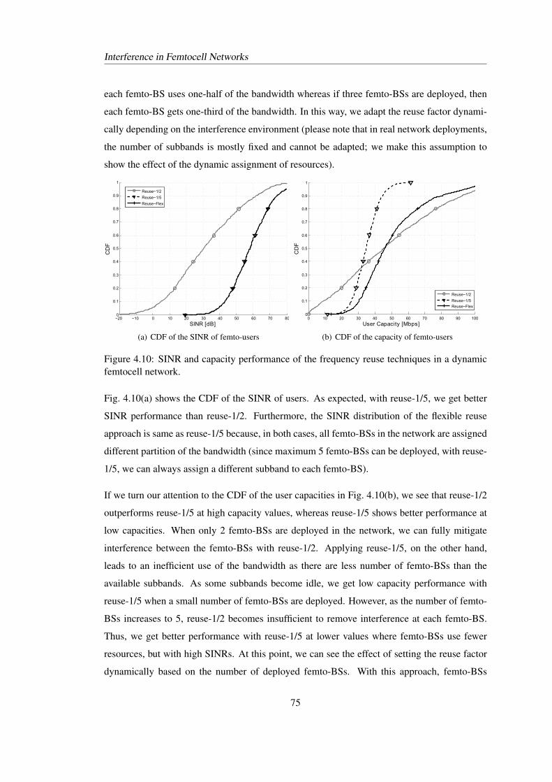
Interference in Femtocell Networks
each femto-BS uses one-half of the bandwidth whereas if three femto-BSs are deployed, then
each femto-BS gets one-third of the bandwidth. In this way, we adapt the reuse factor dynami-
cally depending on the interference environment (please note that in real network deployments,
the number of subbands is mostly fixed and cannot be adapted; we make this assumption to
show the effect of the dynamic assignment of resources).
−20 −10 0 10 20 30 40 50 60 70 800
0.1
0.2
0.3
0.4
0.5
0.6
0.7
0.8
0.9
1
SINR [dB]
CD
F
Reuse−1/2
Reuse−1/5
Reuse−Flex
(a) CDF of the SINR of femto-users
0 10 20 30 40 50 60 70 80 90 1000
0.1
0.2
0.3
0.4
0.5
0.6
0.7
0.8
0.9
1
User/Capacity/[Mbps]
CD
FReuse−1/2
Reuse−1/5
Reuse−Flex
(b) CDF of the capacity of femto-users
Figure 4.10: SINR and capacity performance of the frequency reuse techniques in a dynamicfemtocell network.
Fig. 4.10(a) shows the CDF of the SINR of users. As expected, with reuse-1/5, we get better
SINR performance than reuse-1/2. Furthermore, the SINR distribution of the flexible reuse
approach is same as reuse-1/5 because, in both cases, all femto-BSs in the network are assigned
different partition of the bandwidth (since maximum 5 femto-BSs can be deployed, with reuse-
1/5, we can always assign a different subband to each femto-BS).
If we turn our attention to the CDF of the user capacities in Fig. 4.10(b), we see that reuse-1/2
outperforms reuse-1/5 at high capacity values, whereas reuse-1/5 shows better performance at
low capacities. When only 2 femto-BSs are deployed in the network, we can fully mitigate
interference between the femto-BSs with reuse-1/2. Applying reuse-1/5, on the other hand,
leads to an inefficient use of the bandwidth as there are less number of femto-BSs than the
available subbands. As some subbands become idle, we get low capacity performance with
reuse-1/5 when a small number of femto-BSs are deployed. However, as the number of femto-
BSs increases to 5, reuse-1/2 becomes insufficient to remove interference at each femto-BS.
Thus, we get better performance with reuse-1/5 at lower values where femto-BSs use fewer
resources, but with high SINRs. At this point, we can see the effect of setting the reuse factor
dynamically based on the number of deployed femto-BSs. With this approach, femto-BSs
75
Interference in Femtocell Networks
are assigned more resources if there is a small number of interfering neighbors. In a similar
manner, in dense deployments, the amount of resources assigned to femto-BSs decreases for
higher SINR values. Therefore, the capacity performance with this approach is always better
than reuse-1/5 (right shift of the capacity curve). However, for users having high SINR with
reuse-1/2, diminishing their resources further (in order to improve SINRs of other users) would
cause a decrease on their capacities. Thus, the performance of reuse-1/2 is still better than the
flexible reuse approach at high capacity values.
As a final remark, these simulation results indicate the fact that for the sake of high resource
utilization, there should be a flexibility in the amount of resources assigned to cells where a cell
facing low interference can use more resources with a frequency reuse factor near one.
4.4.2 Enhanced Inter-cell Interference Coordination
As the transmission characteristics of data and control channels are different, most of the tech-
niques used for improving the reception of data channels cannot be applied to the control chan-
nels. For instance, control channels extend over the entire system bandwidth in order to increase
the frequency diversity hence they become more robust to interference. Thus, each BS in the
network uses all bandwidth in the control region whenever they transmit data. Therefore, in-
terference avoidance based on ICIC resource partitioning techniques, in general, can only be
applied to the data region [67]. In such situations, cell-edge users which cannot decode the
control signals because of high interference are still in outage since interfering BSs use the
whole control region even they transmit data over a partition of the data region. In other words,
in LTE and LTE-A, as illustrated in Fig. 4.11, by applying a frequency reuse, we partition the
data region, not the control region.
Control
Subband-1
Subband-2
Subband-3
time
freq.
Figure 4.11: Illustration of resource partitioning during one subframe by considering the controlregions. Note that the control region is used by all BSs in a network, whereas the use ofsubbands in the data region can be coordinated among BSs with the use of the ICIC messages.
To sum up, in order to improve the reception of the control channels, we need specific methods
76
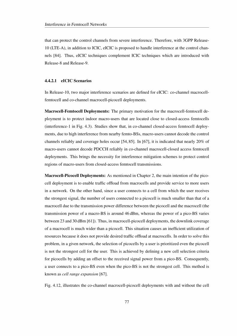
Interference in Femtocell Networks
that can protect the control channels from severe interference. Therefore, with 3GPP Release-
10 (LTE-A), in addition to ICIC, eICIC is proposed to handle interference at the control chan-
nels [84]. Thus, eICIC techniques complement ICIC techniques which are introduced with
Release-8 and Release-9.
4.4.2.1 eICIC Scenarios
In Release-10, two major interference scenarios are defined for eICIC: co-channel macrocell-
femtocell and co-channel macrocell-picocell deployments.
Macrocell-Femtocell Deployments: The primary motivation for the macrocell-femtocell de-
ployment is to protect indoor macro-users that are located close to closed-access femtocells
(interference-1 in Fig. 4.3). Studies show that, in co-channel closed-access femtocell deploy-
ments, due to high interference from nearby femto-BSs, macro-users cannot decode the control
channels reliably and coverage holes occur [54, 85]. In [67], it is indicated that nearly 20% of
macro-users cannot decode PDCCH reliably in co-channel macrocell-closed access femtocell
deployments. This brings the necessity for interference mitigation schemes to protect control
regions of macro-users from closed-access femtocell transmissions.
Macrocell-Picocell Deployments: As mentioned in Chapter 2, the main intention of the pico-
cell deployment is to enable traffic offload from macrocells and provide service to more users
in a network. On the other hand, since a user connects to a cell from which the user receives
the strongest signal, the number of users connected to a picocell is much smaller than that of a
macrocell due to the transmission power difference between the picocell and the macrocell (the
transmission power of a macro-BS is around 46 dBm, whereas the power of a pico-BS varies
between 23 and 30 dBm [61]). Thus, in macrocell-picocell deployments, the downlink coverage
of a macrocell is much wider than a picocell. This situation causes an inefficient utilization of
resources because it does not provide desired traffic offload at macrocells. In order to solve this
problem, in a given network, the selection of picocells by a user is prioritized even the picocell
is not the strongest cell for the user. This is achieved by defining a new cell selection criteria
for picocells by adding an offset to the received signal power from a pico-BS. Consequently,
a user connects to a pico-BS even when the pico-BS is not the strongest cell. This method is
known as cell range expansion [67].
Fig. 4.12, illustrates the co-channel macrocell-picocell deployments with and without the cell
77

Interference in Femtocell Networks
range expansion. In Fig. 4.12(a), users connect to a cell according to the received signal power
and therefore most users connect to the macrocell as they receive the highest power from it.
With the use of the cell range expansion, some users migrate to the picocell due to the offset
value added on the received power from the picocell. Thus, the downlink coverage area of the
picocell expands (shaded area).
(a) without the cell range expansion (b) with the cell range expansion
Figure 4.12: Co-channel macrocell-picocell deployment with and without the cell range expan-sion.
Although the cell range expansion method provides picocells to serve more users and enables
large traffic offloading from macrocells to picocells, the users in the expanded area (shaded
area in Fig. 4.12(b)) face high interference from the macrocell. The reason is that the serving
picocell is not the strongest cell due to the offset value used for the cell selection. Thus, the cell
range expansion results a non-acceptable control channel performance for those users served
by the picocell in the expanded area [53, 86], and the protection of such users constitutes the
second major application area of eICIC.
4.4.2.2 eICIC Approaches
Release-10 offers two different eICIC approaches with a main aim of coordinating interference
at above-mentioned interference scenarios. These two approaches are based on the resource
partitioning among cells. One approach provides the resource partitioning in the frequency do-
main based on carrier-aggregation, whereas the other approach offers the resource partitioning
in the time domain based on the almost blank subframe technique.
Frequency Domain Based eICIC: As mentioned in Chapter 2, in order to provide high data
rates, with LTE-A, a transmission bandwidth up to 100 MHz can be supported. The increase
in the system bandwidth is achieved via carrier aggregation where multiple LTE compatible
frequency bands (component carriers), are combined in order to obtain a wider usable spectrum
up to 100 MHz [20–22]. Therefore, different from LTE, in LTE-A, BSs and users are capable
78
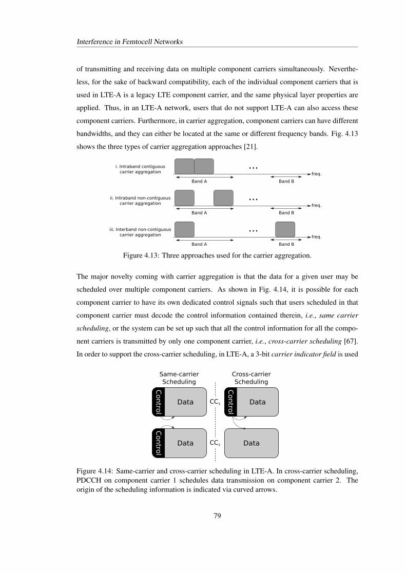
Interference in Femtocell Networks
of transmitting and receiving data on multiple component carriers simultaneously. Neverthe-
less, for the sake of backward compatibility, each of the individual component carriers that is
used in LTE-A is a legacy LTE component carrier, and the same physical layer properties are
applied. Thus, in an LTE-A network, users that do not support LTE-A can also access these
component carriers. Furthermore, in carrier aggregation, component carriers can have different
bandwidths, and they can either be located at the same or different frequency bands. Fig. 4.13
shows the three types of carrier aggregation approaches [21].
freq.
Band A Band B
...i. Intraband contiguous carrier aggregation
freq.
Band A Band B
...ii. Intraband non-contiguous carrier aggregation
freq.
Band A Band B
...iii. Interband non-contiguous carrier aggregation
Figure 4.13: Three approaches used for the carrier aggregation.
The major novelty coming with carrier aggregation is that the data for a given user may be
scheduled over multiple component carriers. As shown in Fig. 4.14, it is possible for each
component carrier to have its own dedicated control signals such that users scheduled in that
component carrier must decode the control information contained therein, i.e., same carrier
scheduling, or the system can be set up such that all the control information for all the compo-
nent carriers is transmitted by only one component carrier, i.e., cross-carrier scheduling [67].
In order to support the cross-carrier scheduling, in LTE-A, a 3-bit carrier indicator field is used
CC1
CC2
Contro
l
Data
Contro
l
Data
Contro
l
Data
Data
Same-carrierScheduling
Cross-carrierScheduling
Figure 4.14: Same-carrier and cross-carrier scheduling in LTE-A. In cross-carrier scheduling,PDCCH on component carrier 1 schedules data transmission on component carrier 2. Theorigin of the scheduling information is indicated via curved arrows.
79
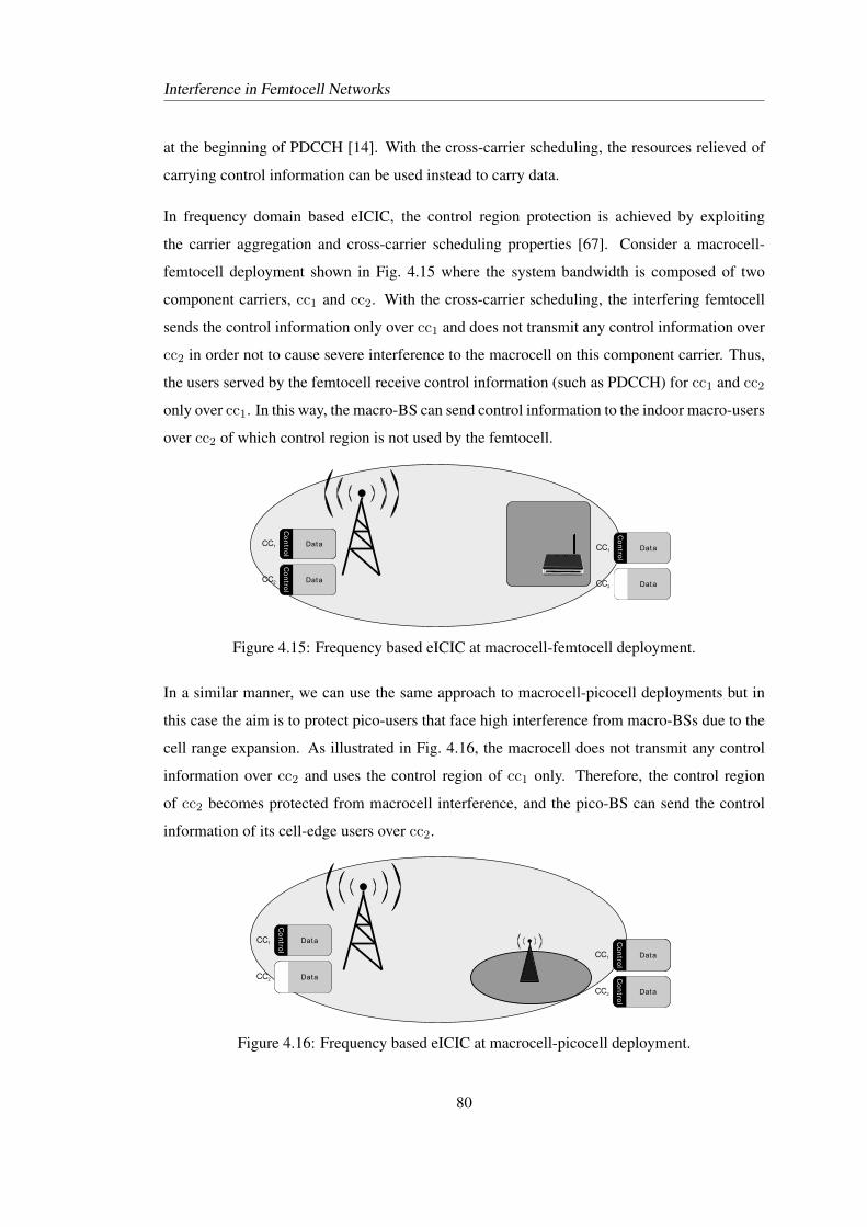
Interference in Femtocell Networks
at the beginning of PDCCH [14]. With the cross-carrier scheduling, the resources relieved of
carrying control information can be used instead to carry data.
In frequency domain based eICIC, the control region protection is achieved by exploiting
the carrier aggregation and cross-carrier scheduling properties [67]. Consider a macrocell-
femtocell deployment shown in Fig. 4.15 where the system bandwidth is composed of two
component carriers, cc1 and cc2. With the cross-carrier scheduling, the interfering femtocell
sends the control information only over cc1 and does not transmit any control information over
cc2 in order not to cause severe interference to the macrocell on this component carrier. Thus,
the users served by the femtocell receive control information (such as PDCCH) for cc1 and cc2
only over cc1. In this way, the macro-BS can send control information to the indoor macro-users
over cc2 of which control region is not used by the femtocell.
Control
Data
Data
CC1
CC2Control
Data
CC1
CC2
Data
Control
Data
Figure 4.15: Frequency based eICIC at macrocell-femtocell deployment.
In a similar manner, we can use the same approach to macrocell-picocell deployments but in
this case the aim is to protect pico-users that face high interference from macro-BSs due to the
cell range expansion. As illustrated in Fig. 4.16, the macrocell does not transmit any control
information over cc2 and uses the control region of cc1 only. Therefore, the control region
of cc2 becomes protected from macrocell interference, and the pico-BS can send the control
information of its cell-edge users over cc2.
Control
Data
Data
CC1
CC2 Control
Data
CC1
CC2
Data
Control
Data
Figure 4.16: Frequency based eICIC at macrocell-picocell deployment.
80
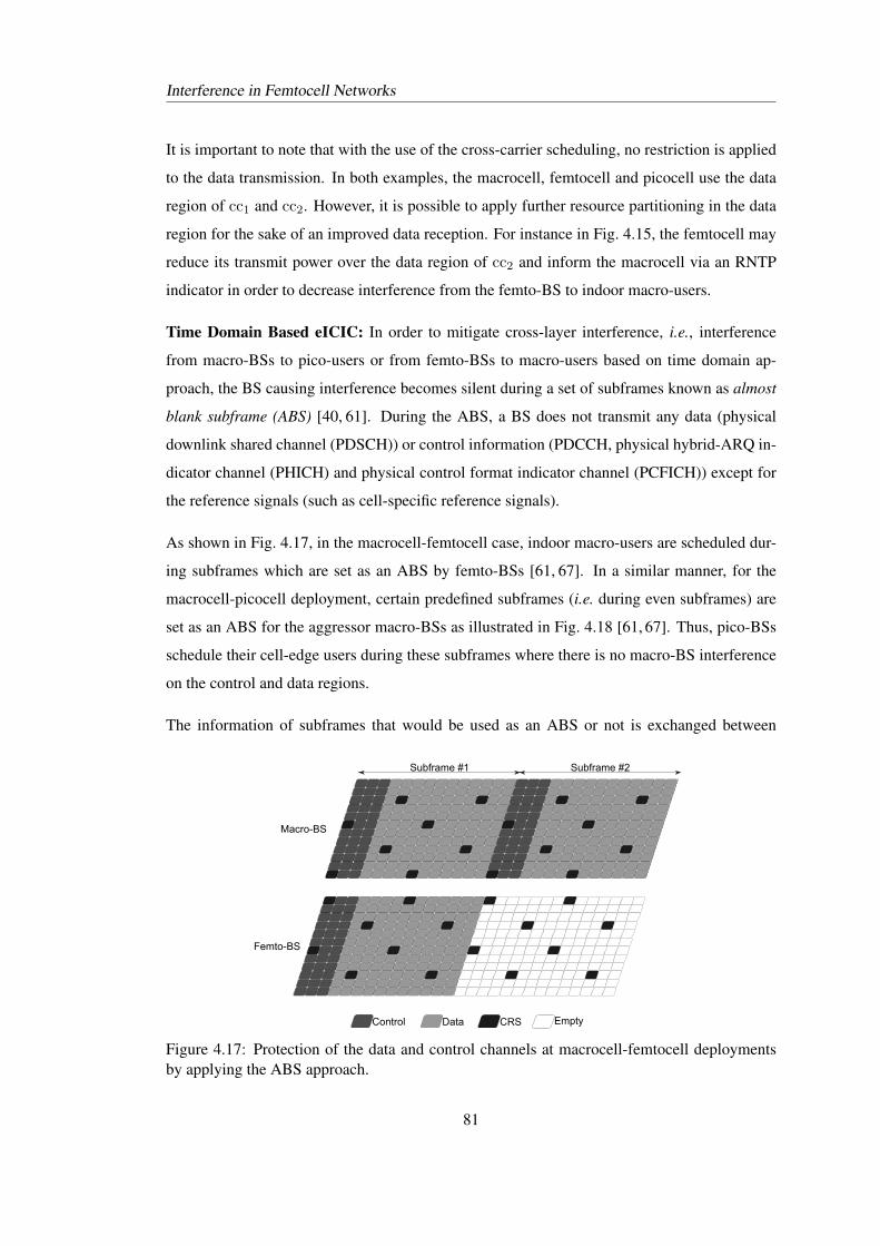
Interference in Femtocell Networks
It is important to note that with the use of the cross-carrier scheduling, no restriction is applied
to the data transmission. In both examples, the macrocell, femtocell and picocell use the data
region of cc1 and cc2. However, it is possible to apply further resource partitioning in the data
region for the sake of an improved data reception. For instance in Fig. 4.15, the femtocell may
reduce its transmit power over the data region of cc2 and inform the macrocell via an RNTP
indicator in order to decrease interference from the femto-BS to indoor macro-users.
Time Domain Based eICIC: In order to mitigate cross-layer interference, i.e., interference
from macro-BSs to pico-users or from femto-BSs to macro-users based on time domain ap-
proach, the BS causing interference becomes silent during a set of subframes known as almost
blank subframe (ABS) [40, 61]. During the ABS, a BS does not transmit any data (physical
downlink shared channel (PDSCH)) or control information (PDCCH, physical hybrid-ARQ in-
dicator channel (PHICH) and physical control format indicator channel (PCFICH)) except for
the reference signals (such as cell-specific reference signals).
As shown in Fig. 4.17, in the macrocell-femtocell case, indoor macro-users are scheduled dur-
ing subframes which are set as an ABS by femto-BSs [61, 67]. In a similar manner, for the
macrocell-picocell deployment, certain predefined subframes (i.e. during even subframes) are
set as an ABS for the aggressor macro-BSs as illustrated in Fig. 4.18 [61, 67]. Thus, pico-BSs
schedule their cell-edge users during these subframes where there is no macro-BS interference
on the control and data regions.
The information of subframes that would be used as an ABS or not is exchanged between
Control Data CRS Empty
Subframe #1 Subframe #2
Macro-BS
Femto-BS
Figure 4.17: Protection of the data and control channels at macrocell-femtocell deploymentsby applying the ABS approach.
81
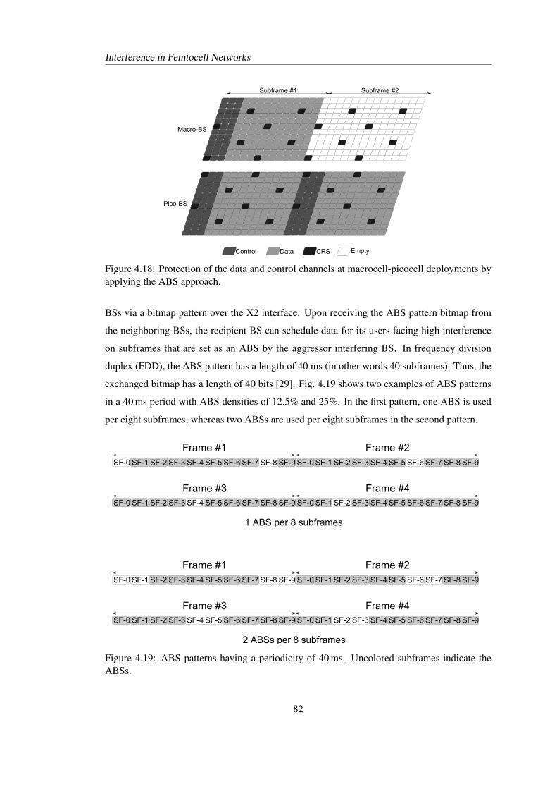
Interference in Femtocell Networks
Control Data CRS Empty
Subframe #1 Subframe #2
Macro-BS
Pico-BS
Figure 4.18: Protection of the data and control channels at macrocell-picocell deployments byapplying the ABS approach.
BSs via a bitmap pattern over the X2 interface. Upon receiving the ABS pattern bitmap from
the neighboring BSs, the recipient BS can schedule data for its users facing high interference
on subframes that are set as an ABS by the aggressor interfering BS. In frequency division
duplex (FDD), the ABS pattern has a length of 40 ms (in other words 40 subframes). Thus, the
exchanged bitmap has a length of 40 bits [29]. Fig. 4.19 shows two examples of ABS patterns
in a 40 ms period with ABS densities of 12.5% and 25%. In the first pattern, one ABS is used
per eight subframes, whereas two ABSs are used per eight subframes in the second pattern.
Frame #1SF-6 SF-7SF-4 SF-5SF-2 SF-3SF-0 SF-1 SF-8 SF-9 SF-6 SF-7SF-4 SF-5SF-2 SF-3SF-0 SF-1 SF-8 SF-9
Frame #2
SF-6 SF-7SF-4 SF-5SF-2 SF-3SF-0 SF-1 SF-8 SF-9 SF-6 SF-7SF-4 SF-5SF-2 SF-3SF-0 SF-1 SF-8 SF-9
Frame #3 Frame #4
1 ABS per 8 subframes
Frame #1SF-6 SF-7SF-4 SF-5SF-2 SF-3SF-0 SF-1 SF-8 SF-9 SF-6 SF-7SF-4 SF-5SF-2 SF-3SF-0 SF-1 SF-8 SF-9
Frame #2
SF-6 SF-7SF-4 SF-5SF-2 SF-3SF-0 SF-1 SF-8 SF-9 SF-6 SF-7SF-4 SF-5SF-2 SF-3SF-0 SF-1 SF-8 SF-9
Frame #3 Frame #4
2 ABSs per 8 subframes
Figure 4.19: ABS patterns having a periodicity of 40 ms. Uncolored subframes indicate theABSs.
82
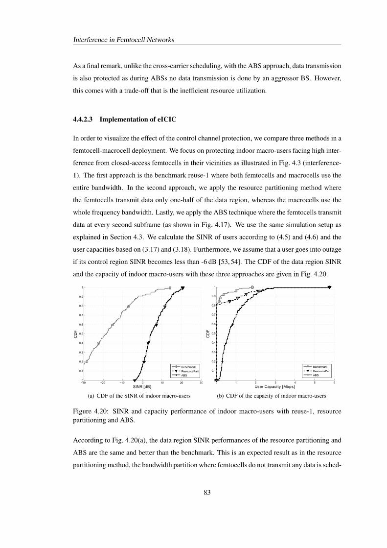
Interference in Femtocell Networks
As a final remark, unlike the cross-carrier scheduling, with the ABS approach, data transmission
is also protected as during ABSs no data transmission is done by an aggressor BS. However,
this comes with a trade-off that is the inefficient resource utilization.
4.4.2.3 Implementation of eICIC
In order to visualize the effect of the control channel protection, we compare three methods in a
femtocell-macrocell deployment. We focus on protecting indoor macro-users facing high inter-
ference from closed-access femtocells in their vicinities as illustrated in Fig. 4.3 (interference-
1). The first approach is the benchmark reuse-1 where both femtocells and macrocells use the
entire bandwidth. In the second approach, we apply the resource partitioning method where
the femtocells transmit data only one-half of the data region, whereas the macrocells use the
whole frequency bandwidth. Lastly, we apply the ABS technique where the femtocells transmit
data at every second subframe (as shown in Fig. 4.17). We use the same simulation setup as
explained in Section 4.3. We calculate the SINR of users according to (4.5) and (4.6) and the
user capacities based on (3.17) and (3.18). Furthermore, we assume that a user goes into outage
if its control region SINR becomes less than -6 dB [53, 54]. The CDF of the data region SINR
and the capacity of indoor macro-users with these three approaches are given in Fig. 4.20.
−30 −20 −10 0 10 20 300
0.1
0.2
0.3
0.4
0.5
0.6
0.7
0.8
0.9
1
SINRs[dB]
CD
F
Benchmark
ResourcePart
ABS
(a) CDF of the SINR of indoor macro-users
0 1 2 3 4 5 60
0.1
0.2
0.3
0.4
0.5
0.6
0.7
0.8
0.9
1
UserhCapacityh[Mbps]
CD
F
Benchmark
ResourcePart
ABS
(b) CDF of the capacity of indoor macro-users
Figure 4.20: SINR and capacity performance of indoor macro-users with reuse-1, resourcepartitioning and ABS.
According to Fig. 4.20(a), the data region SINR performances of the resource partitioning and
ABS are the same and better than the benchmark. This is an expected result as in the resource
partitioning method, the bandwidth partition where femtocells do not transmit any data is sched-
83
Interference in Femtocell Networks
uled to indoor macro-users. Similarly, in the ABS technique, macrocells schedule their indoor
users during subframes which are set as an ABS by femtocells. Thus, in both approaches, inter-
ference from femtocells to indoor macro-users is mitigated. However, we can see the superiority
of the ABS technique to the resource partitioning when we compare the capacity performance
of these methods in Fig. 4.20(b). Since the control channels are not protected in the resource
partitioning, all BSs use the control region without any restriction. Thus, the indoor macro-
users go into outage even they experience high SINR at the data region. That is why the outage
ratios of the benchmark and resource partitioning approaches are the same irrelevant of the data
region SINR performance. For the rest users that can decode the control channels, we can see
the improvement in the user capacity with the resource partitioning approach due to the mitiga-
tion of interference from the femtocells. On the other hand, with the ABS technique, we protect
both the control and data channels, thus the improvement in the data region SINR matches with
the improvement of the user capacity values where no indoor macro-user is in outage anymore.
Although the proposed eICIC techniques solve the control channel interference issue with a
low complexity, the focus is given on mitigating cross-layer interference between macrocell
- femtocell or macrocell - picocell. As all pico and femto-BSs use the same time and fre-
quency resources, the proposed methods do not offer any solution to reduce co-layer interfer-
ence. However, in dense deployments, interference between femtocells, and between picocells
requires more attention. Furthermore, in the ABS approach, as the ABS configurations of BSs
are considered static, no adaptation to variable interference conditions is offered. This even-
tually decreases the utilization efficiency of the resources since BSs do not transmit any data
during ABSs. Thus, further improvements are required for mitigating interference between
femtocells.
4.4.3 User and BS Measurements
Until now, the messages required for coordination between BSs have been discussed. For
an efficient interference management, it is also important for users to sense the environment
and report it to their serving cells. There are some feedback mechanisms available in LTE
and LTE-A where users can provide information to their serving cells regarding the channel
conditions and potential interferers.
One of the fundamental signaling used in LTE and LTE-A is the channel-quality indicator
(CQI) feedback where a user reports the SINR level of a channel to its serving BS in terms of
84
Interference in Femtocell Networks
suitable modulation and coding scheme [71]. With the help of the CQI reports, a serving BS
can choose the most appropriate modulation scheme and code rate for each user depending on
the channel conditions. Low-order modulations, such as quadrature phase-shift keying (QPSK),
are more robust to interference but carry less information. On the other hand, high-order mod-
ulations, such as 64-quadrature amplitude modulation (QAM), offer higher bit rates but they
are more sensitive to interference and channel estimations. Similarly, the code rates can also
be adapted according to the channel conditions. In the high interference case, a low code rate
is applied providing low efficiency in terms of a bit rate but robustness to strong interference.
However, if the channel conditions are good, then a large code rate is used to obtain high data
rates. In this way, a BS can optimize the use of resources by applying the modulation and
coding scheme according to the varying channel conditions [14].
CQI information is calculated according to the SINR experienced by a user. A CQI report
includes the highest modulation and coding scheme that the user can use based on the measured
received signal quality where the maximum error rate probability should not exceed 10% [14].
According to the 3GPP specifications, a user reports 16 different modulation schemes and code
rates. Each combination of the modulation scheme and the code rate is represented by an index
ranging from 0 to 15 [71].
There are three types of CQI reports; wideband reporting, BS-configured subband reporting and
user selected subband reporting [29]. In the wideband CQI report, a user makes a measurement
over the whole bandwidth. In the BS-based CQI report, a user makes measurements over sub-
bands (part of the bandwidth consisted of a predefined number of contiguous resource blocks)
and report the CQI for each subband asked by its serving BS. In the user selected CQI report,
a user makes measurements over subbands like the BS-based report, but it generates only one
CQI report based on the set of subbands which are chosen by the user. For a wideband CQI, as
16 values are available, 4-bit report is used [87]. BS-based and user selected CQI reports, on
the other hand, are encoded differentially with respect to their respective wideband CQI values.
For instance, for a BS-based CQI value, only 2 bits are used for each subband [71].
CQI reporting can be aperiodic or periodic. The aperiodic CQI report is requested by a serving
BS, and the minimum reporting period of a CQI report is one subframe [71]. In the periodic re-
porting, a user can only report the wideband and user selected reporting schemes. Furthermore,
a user can report a wideband CQI with a period of: 2, 5, 10, 16, 20, 32, 40, 64, 80, 128 ms [14].
85
Interference in Femtocell Networks
As the CQI report indicates the channel conditions, it can also be used for the interference
management. With the help of the CQI reports, a serving BS is aware of which user faces
high interference over which subband. Thus, the BS can make an efficient frequency selective
scheduling. It is clear that the performance of the resource scheduling would increase with the
frequent CQI reporting. In this way, the serving BS can track the variations in the channel.
Also, increasing the granularity in the bandwidth (i.e. increasing the number of subbands that
a user reports), gives a better scheduling opportunities and flexibility to the serving BS. On the
other hand, the trade-off is the increased signaling overhead in the uplink direction. In LTE and
LTE-A, BSs can update the frequency of the CQI reports and the subband size depending on
the network conditions, i.e. increasing the reporting frequency when there are large fluctuations
in the channel.
Another user report defined in 3GPP is the reference signal received power (RSRP) which
stands for the signal strength of a BS measured by a user. In LTE and LTE-A, a user can
measure the received signals from various BSs in its vicinity with the help of cell-specific
reference signals. Then, it sends a measurement report, which includes the identities of the
most dominant BSs in its vicinity along with the associated RSRPs, to its serving BS [88].
The RSRP is used for cell selection/reselection, handover and estimating the path loss for power
calculations [29]. Therefore, it is one of the most crucial signaling in LTE and LTE-A. A user
can perform RSRP measurements of 8 identified intra-frequency cells at a given time [89]. The
measurement period of the RSRP for the intra-frequency measurements is 200 ms [14]. The
RSRP values are reported with a 1 dB resolution ranging from -140 dBm to -44 dBm, and these
values are mapped onto an integer value between 0 and 97 [89].
As RSRP reports indicate the signal strength from the neighboring BSs, with these reports the
serving BS has information about the interfering environment of each user and can use these
reports for supporting the interference management in LTE and LTE-A networks.
In addition to users, in LTE and LTE-A, femto-BSs are also capable of sensing the environ-
ment and measuring interference from neighboring BSs. Such measurement is achieved by
implementing a downlink receiver also known as BS-sniffer [90]. With the help of the sniffing
technique, a femto-BS can listen its environment during downlink transmissions. Thus, it can
get more information about its local area (such as cell identities, received signal strength, and
access policies of neighboring cells) to improve its decisions on the resource assignment.
86
Interference in Femtocell Networks
4.4.4 MIMO and CoMP Techniques
In addition to the ICIC and eICIC techniques, LTE and LTE-A networks also offer another
interference mitigation techniques that have different application areas depending on the in-
terference situation. Operators choose the appropriate method depending on the deployment
scenario such as backhaul performance, and hardware availability. These approaches can be
used exclusively or applied together at some extent to complement each other to get a better
performance [91].
One of the commonly used techniques is multiple antenna techniques also known as multiple-
input and multiple-output (MIMO). With MIMO, interference can be reduced through provid-
ing additional diversity against fading on the channel. Thus, the robustness of the transmit-
ted/received signal is increased. Another interference handling method that can be used with
multi-antennas is to direct the antenna beam to the desired transmitter/receiver to maximize the
antenna gain also known as beamforming.
MIMO techniques can also be applied to Het-Nets. However, these techniques give better
results under high SINR conditions with accurate channel estimations. Furthermore, some
MIMO techniques including spatial multiplexing are only available for the data transmission
as the control channels have different transmission schemes than that of the data channels.
Nevertheless, applying such techniques with ICIC and eICIC offers more effective interference
mitigation. In this work, we will give our focus mostly on the resource partitioning via ICIC
and eICIC techniques and leave the application of the MIMO techniques to femtocell networks
as a future work.
Another technique, known as coordinated multi-point (CoMP), has gained significant improve-
ment both in academy and industry and it is planned to be commercialized for future LTE-A
deployments. The idea of CoMP is the cooperation of BSs in terms of transmission and/or
reception in order to improve the system performance especially at cell edges. By definition,
CoMP covers a broad variety of techniques such as MIMO and ICIC. Fig. 4.21 shows differ-
ent variations of CoMP, which are coordinated scheduling, coordinated beamforming and joint
transmission [14].
Coordinated scheduling is the simplest form of CoMP where the interfering cell reduces the
transmission power (or does not transmit) over the resources that are reserved for the cell-edge
users of neighboring cells. This version of CoMP compromises the ICIC used for the resource
87
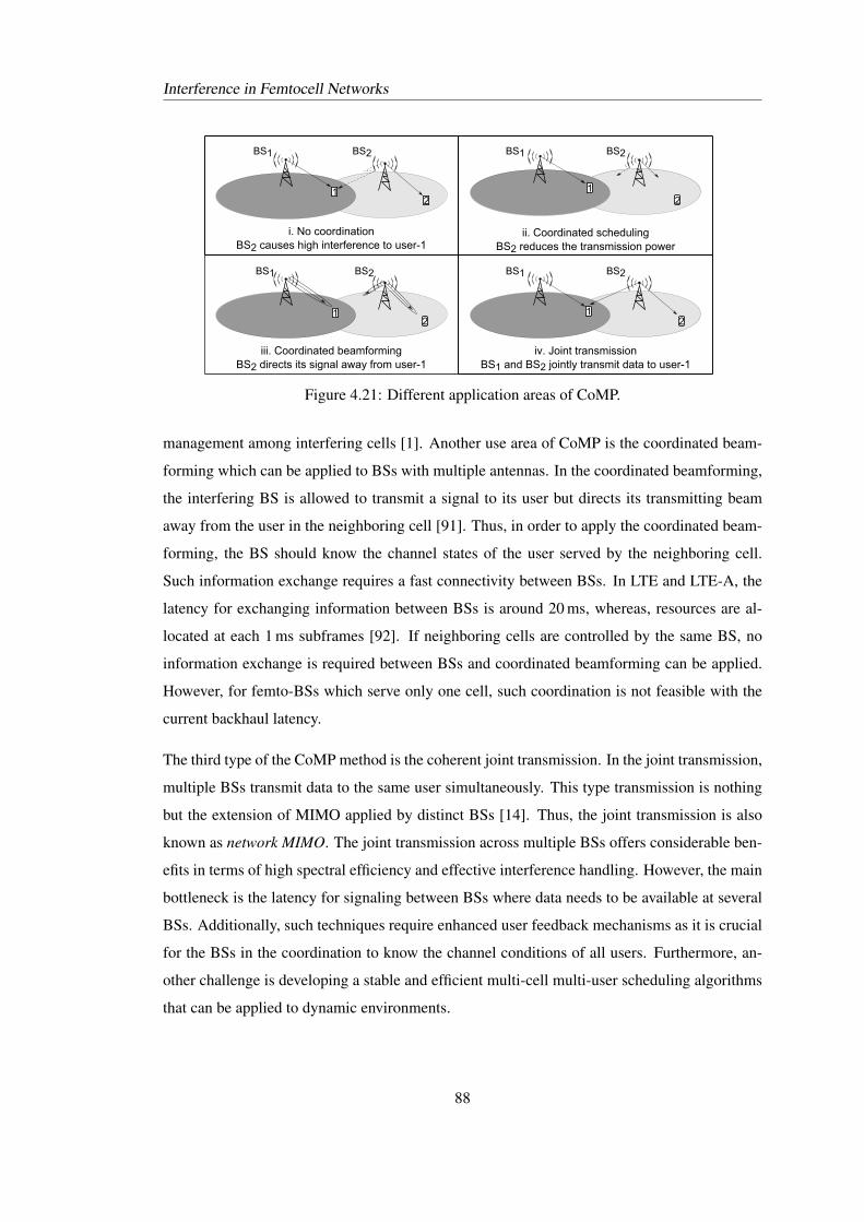
Interference in Femtocell Networks
i.jNojcoordinationBS2jcausesjhighjinterferencejtojuser-1j
ii.jCoordinatedjschedulingBS2jreducesjthejtransmissionjpower
iii.jCoordinatedjbeamformingBS2jdirectsjitsjsignaljawayjfromjuser-1
BS1 BS2 BS1 BS2
iv.jJointjtransmissionBS1jandjBS2jjointlyjtransmitjdatajtojuser-1
BS1 BS2BS1 BS2
1
1 1
12
22
2
Figure 4.21: Different application areas of CoMP.
management among interfering cells [1]. Another use area of CoMP is the coordinated beam-
forming which can be applied to BSs with multiple antennas. In the coordinated beamforming,
the interfering BS is allowed to transmit a signal to its user but directs its transmitting beam
away from the user in the neighboring cell [91]. Thus, in order to apply the coordinated beam-
forming, the BS should know the channel states of the user served by the neighboring cell.
Such information exchange requires a fast connectivity between BSs. In LTE and LTE-A, the
latency for exchanging information between BSs is around 20 ms, whereas, resources are al-
located at each 1 ms subframes [92]. If neighboring cells are controlled by the same BS, no
information exchange is required between BSs and coordinated beamforming can be applied.
However, for femto-BSs which serve only one cell, such coordination is not feasible with the
current backhaul latency.
The third type of the CoMP method is the coherent joint transmission. In the joint transmission,
multiple BSs transmit data to the same user simultaneously. This type transmission is nothing
but the extension of MIMO applied by distinct BSs [14]. Thus, the joint transmission is also
known as network MIMO. The joint transmission across multiple BSs offers considerable ben-
efits in terms of high spectral efficiency and effective interference handling. However, the main
bottleneck is the latency for signaling between BSs where data needs to be available at several
BSs. Additionally, such techniques require enhanced user feedback mechanisms as it is crucial
for the BSs in the coordination to know the channel conditions of all users. Furthermore, an-
other challenge is developing a stable and efficient multi-cell multi-user scheduling algorithms
that can be applied to dynamic environments.
88
Interference in Femtocell Networks
4.5 The Way Forward
Starting from the next chapter, for interference management in femtocell networks, we con-
sider interference avoidance approaches based on the resource partitioning among BSs. Thus,
depending on the interference environment, BSs cooperate with each other, and they give up
some of their resources in return for low interference on other resources. For this purpose, we
develop techniques mainly based on ICIC and eICIC provided by LTE and LTE-A networks.
The reason we focus on the ICIC and eICIC techniques is that their suitability to femtocell net-
works as they do not require advanced hardware or complicated algorithms at terminals. Also,
the resource partitioning does not require real time coordination between BSs and they can bare
delay in information exchange between BSs.
For an efficient interference handling performance in femtocell networks, we aim for a dynamic
resource partitioning method with high resource utilization. The resource assignment should
depend on the current interference environment and be updated according to the variations at the
interference environment such as the change of the number of BSs, location of users, required
data traffic.
The drawback of the resource partitioning would be seen as the less efficient use of resources
with respect to reuse-1 deployments that may cause a decrease in the overall system through-
put [70, 92]. However, with the femtocell deployment, thanks to the significant increase in the
spatial reuse of resources, more resources are available for users (with the same available band-
width, macrocells serve to users in the order of tens, however femtocells serve only couple of
users), and some of them can be remained idle for the sake of high cell-edge performances.
Apart from this, with smart and novel resource management techniques, interference problems
can be solved with high resource utilization.
In a general sense, we can classify our work into two groups; interference mitigation at the
control region and the data region. For the control region interference mitigation, we stick to
the LTE and LTE-A specifications and develop techniques considering the network constraints.
For the data region interference mitigation, we relax our network constraints and seek for the
high cell-edge user performance in terms of data rates.
We further classify the data region interference mitigation into two approaches; central and
distributed approach [93]. In the central approach, there is a central controller which can be an
HeNB-gateway (HeNB-GW) or one of the BSs in a network, and it is responsible for assigning
89
Interference in Femtocell Networks
resources to BSs or users. On the other hand, in the distributed approach, BSs assign resources
autonomously by using feedback from neighboring cells and users. Both approaches have their
own advantages and drawbacks. The major advantage of the central approach is that the central
controller has global information and can make an efficient resource assignment based on the
given requirements, whereas, in the distributed approach, each BS has its local information.
Also, with the central approach, a stable resource assignment is reached shortly. However, in the
distributed approach, each BS makes its own decision simultaneously; thus, multiple iterations
are needed by the BSs to reach a stable resource assignment. Therefore, with the distributed
approach, BSs would take wrong actions thereby causing the system to become unstable. The
central approach, on the other hand, brings high complexity at the central controller. In the
distributed approach, since the decisions are taken by each BSs autonomously, the complexity
is shared among the BSs.
4.6 Conclusion
Interference handling techniques and their applications to femtocell networks are discussed in
this chapter. Using the simulation results, we show that interference between femtocells is more
significant than interference between a macrocell and a femtocell. Thus, we give our attention
mainly to femtocell networks.
Because of its very nature, we need to develop an interference management technique specific
to femtocell networks. First and foremost, the interference mitigation technique should update
itself dynamically with respect to the changes in the interference environment. Also, it should
be resource efficient and should provide high performances with modest signaling overhead.
The performance of an interference handling technique depends on the frequency of feedback
that a BS gets from its users and other BSs. On the other hand, due to hardware and backhaul
limitations, methods developed for macrocell networks do not achieve the same performance in
femtocell networks. Taking such restrictions into account, we consider the resource partitioning
via coordination between cells as a promising candidate since implementing such a technique
is less complicated than other interference management techniques in terms of the hardware
requirements and the signaling overhead.
Although the theoretical methods provide significant gains, due to their complexity, they cannot
be applied to real networks. As we seek for a more practical solution, we focus on methods that
90
Interference in Femtocell Networks
can be used in LTE and LTE-A networks. Thus, we explain the ICIC and eICIC techniques that
are supported by LTE and LTE-A. We also discuss the interference mitigation of the control
and data channels and the available solutions. With the help of the simulation results, we
show that the current approaches are not enough to deal with interference in dynamic femtocell
networks. Thus, starting from the next chapter, we introduce interference handling methods
that are applicable to such networks.
91
Interference in Femtocell Networks
92
Chapter 5Control Channel Protection in LTE and
LTE-A Networks
5.1 Introduction
In every subframe, which is the basic time-domain unit for downlink and uplink scheduling,
the data transmission is preceded by the transmission of the control channels such as physical
downlink control channel (PDCCH), physical hybrid-ARQ indicator channel (PHICH) and
physical control format indicator channel (PCFICH). Correct reception of the control channels
is particularly important for Long-Term Evolution (LTE) and Long-Term Evolution-Advanced
(LTE-A) networks because the control channels, which, among other things, point the users to
their assigned data channels in the frequency domain. It must be noted that corrupted reception
of the control channels will necessarily result in a loss of the subsequent data in that subframe
and results in a service outage. In other words, the control channels should be robust against
high interference in order to achieve a reliable cell coverage. Thus, processing techniques
(such as coding, modulation and mapping of symbols to the frequency domain) of the control
channels are different from those applied to the data channels. Therefore, different techniques
are required in order to protect the control regions of each subframe.
Most of the existing studies in the literature focus on data channel interference mitigation be-
tween cells to improve the data rates of cell-edge users. However, as shown in Chapter 4, the
improvements in the data channel performance cannot be realized unless the performance of
93
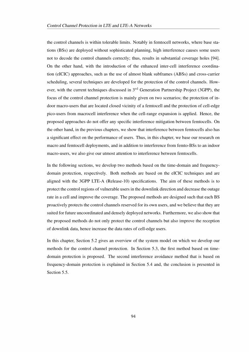
Control Channel Protection in LTE and LTE-A Networks
the control channels is within tolerable limits. Notably in femtocell networks, where base sta-
tions (BSs) are deployed without sophisticated planning, high interference causes some users
not to decode the control channels correctly; thus, results in substantial coverage holes [94].
On the other hand, with the introduction of the enhanced inter-cell interference coordina-
tion (eICIC) approaches, such as the use of almost blank subframes (ABSs) and cross-carrier
scheduling, several techniques are developed for the protection of the control channels. How-
ever, with the current techniques discussed in 3rd Generation Partnership Project (3GPP), the
focus of the control channel protection is mainly given on two scenarios; the protection of in-
door macro-users that are located closed vicinity of a femtocell and the protection of cell-edge
pico-users from macrocell interference when the cell-range expansion is applied. Hence, the
proposed approaches do not offer any specific interference mitigation between femtocells. On
the other hand, in the previous chapters, we show that interference between femtocells also has
a significant effect on the performance of users. Thus, in this chapter, we base our research on
macro and femtocell deployments, and in addition to interference from femto-BSs to an indoor
macro-users, we also give our utmost attention to interference between femtocells.
In the following sections, we develop two methods based on the time-domain and frequency-
domain protection, respectively. Both methods are based on the eICIC techniques and are
aligned with the 3GPP LTE-A (Release-10) specifications. The aim of these methods is to
protect the control regions of vulnerable users in the downlink direction and decrease the outage
rate in a cell and improve the coverage. The proposed methods are designed such that each BS
proactively protects the control channels reserved for its own users, and we believe that they are
suited for future uncoordinated and densely deployed networks. Furthermore, we also show that
the proposed methods do not only protect the control channels but also improve the reception
of downlink data, hence increase the data rates of cell-edge users.
In this chapter, Section 5.2 gives an overview of the system model on which we develop our
methods for the control channel protection. In Section 5.3, the first method based on time-
domain protection is proposed. The second interference avoidance method that is based on
frequency-domain protection is explained in Section 5.4 and, the conclusion is presented in
Section 5.5.
94
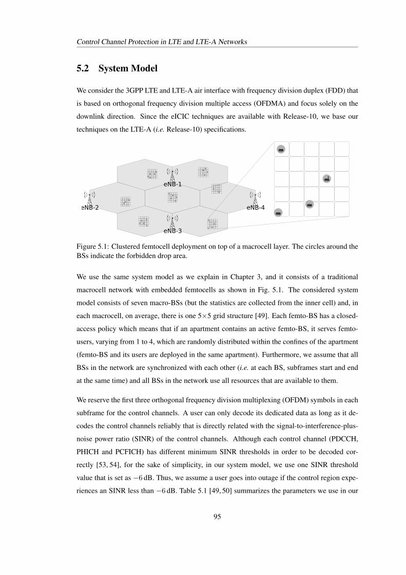
Control Channel Protection in LTE and LTE-A Networks
5.2 System Model
We consider the 3GPP LTE and LTE-A air interface with frequency division duplex (FDD) that
is based on orthogonal frequency division multiple access (OFDMA) and focus solely on the
downlink direction. Since the eICIC techniques are available with Release-10, we base our
techniques on the LTE-A (i.e. Release-10) specifications.
eNB-1
eNB-2
eNB-3
eNB-4
Figure 5.1: Clustered femtocell deployment on top of a macrocell layer. The circles around theBSs indicate the forbidden drop area.
We use the same system model as we explain in Chapter 3, and it consists of a traditional
macrocell network with embedded femtocells as shown in Fig. 5.1. The considered system
model consists of seven macro-BSs (but the statistics are collected from the inner cell) and, in
each macrocell, on average, there is one 5×5 grid structure [49]. Each femto-BS has a closed-
access policy which means that if an apartment contains an active femto-BS, it serves femto-
users, varying from 1 to 4, which are randomly distributed within the confines of the apartment
(femto-BS and its users are deployed in the same apartment). Furthermore, we assume that all
BSs in the network are synchronized with each other (i.e. at each BS, subframes start and end
at the same time) and all BSs in the network use all resources that are available to them.
We reserve the first three orthogonal frequency division multiplexing (OFDM) symbols in each
subframe for the control channels. A user can only decode its dedicated data as long as it de-
codes the control channels reliably that is directly related with the signal-to-interference-plus-
noise power ratio (SINR) of the control channels. Although each control channel (PDCCH,
PHICH and PCFICH) has different minimum SINR thresholds in order to be decoded cor-
rectly [53, 54], for the sake of simplicity, in our system model, we use one SINR threshold
value that is set as −6 dB. Thus, we assume a user goes into outage if the control region expe-
riences an SINR less than −6 dB. Table 5.1 [49, 50] summarizes the parameters we use in our
95
Control Channel Protection in LTE and LTE-A Networks
Parameter Value
Number of Tx antennas 1
Number of Rx antennas 1
RB bandwidth 180 kHz
OFDMA symbols per slot 7 - normal cyclic prefix is applied
Size of the control region fixed at 3 OFDM symbols
Minimum SINR for decoding controlsignals
−6 dB
Sector per site 3
Macro-users per cell 10 (on average)
5×5 grids per cell 1 (on average)
Apartment dimensions 10m× 10m
Femto-BS activation probability 0.2
Femto-users per active femto-BS variable between 1 and 4
Table 5.1: System model assumptions.
simulations.
In simulations, we use two metrics; the user SINR and capacity. We calculate the average SINR
of user u as
γu =
∑n∈Nu
γnu
|Nu|, (5.1)
where Nu is the set of resource blocks scheduled to u and γnu is the SINR of resource block n
experienced by u. We calculate the SINR of resource block n experienced by user u served by
BS b as
γnu =Pnu,b∑
i∈IuPnu,i + ηRB
, (5.2)
where Pnu,b is the received signal power from the serving BS, Pnu,i is the interfering power from
BS i, Iu is the set of interfering BSs including both femto and macro-BSs in the simulation
area and ηRB is the sum effect of the thermal noise and user receiver noise over the bandwidth
of one resource block.
We use the attenuated and truncated Shannon bound method [52] for the user capacity calcula-
96
Control Channel Protection in LTE and LTE-A Networks
tions. The spectral efficiency of user u on resource block n in [bps/Hz] is calculated as [52]
Rnu =
0 for γnu [dB] < −10
0.6log2(1 + γnu ) for −10 6 γnu [dB] 6 22
4.4 for γnu [dB] > 22
(5.3)
where γnu is the SINR of resource block n experienced by u, 0.6 is the attenuation factor which
represents implementation losses, −10 and 22 dB are the minimum and maximum SINRs used
by the available modulation and coding schemes. It is assumed that a reliable data transmission
can be achieved for SINR values less than −10 dB. On the other hand, due to a limitation of
the applied modulation and coding schemes, no further improvement in the spectral efficiency
can be achieved for SINR values higher than 22 dB. Therefore, in (5.3), the upper limit for the
achievable spectral efficiency is 4.4 bps/Hz that is calculated based on an SINR value of 22 dB.
Given the set Nu of resource blocks allocated to user u, the capacity Cu of user u is calculated
as
Cu =∑n∈Nu
BeffBRBRnu, (5.4)
where BRB is the bandwidth of a resource block and Beff is the bandwidth efficiency. As we
mention in Chapter 3, Beff stands for the ratio of the bandwidth used for data transmissions
after the cyclic prefix insertion and the control channels and reference signals allocation. Thus,
it depends on the bandwidth and the number of OFDM symbols used for the control region.
All parameters are based on the 3GPP specifications and are summarized in Table 5.2 [49, 50].
5.3 Protection of Cell-Edge Users via Almost Blank Subframes
We develop an interference mitigation technique that is based on time-domain protection by
using the ABS approach [40, 61]. An ABS is a subframe during which a BS does not transmit
any data but only reference signals. In order to refresh our knowledge on the control channels
and the use of ABSs, we refer to Fig. 5.2 that gives an overview of the data and control channels
and cell-specific reference signals (CRSs) transmitted during a normal subframe and an ABS
by assuming three OFDM symbols are used for the control region.
As we discuss in Chapter 4, the proposed ABS scheme in 3GPP focuses on cross-layer interfer-
ence between macrocells and femtocells. It does not offer any protection between femtocells
97
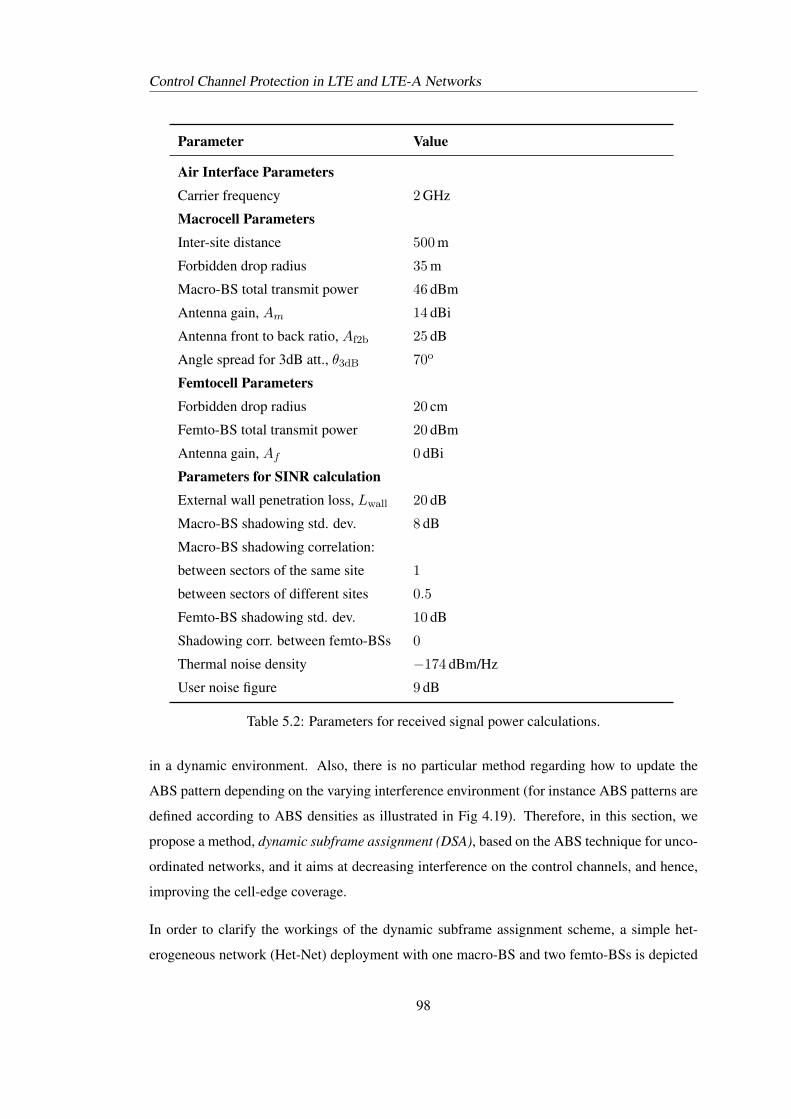
Control Channel Protection in LTE and LTE-A Networks
Parameter Value
Air Interface ParametersCarrier frequency 2 GHz
Macrocell ParametersInter-site distance 500 m
Forbidden drop radius 35 m
Macro-BS total transmit power 46 dBm
Antenna gain, Am 14 dBi
Antenna front to back ratio, Af2b 25 dB
Angle spread for 3dB att., θ3dB 70o
Femtocell ParametersForbidden drop radius 20 cm
Femto-BS total transmit power 20 dBm
Antenna gain, Af 0 dBi
Parameters for SINR calculationExternal wall penetration loss, Lwall 20 dB
Macro-BS shadowing std. dev. 8 dB
Macro-BS shadowing correlation:
between sectors of the same site 1
between sectors of different sites 0.5
Femto-BS shadowing std. dev. 10 dB
Shadowing corr. between femto-BSs 0
Thermal noise density −174 dBm/Hz
User noise figure 9 dB
Table 5.2: Parameters for received signal power calculations.
in a dynamic environment. Also, there is no particular method regarding how to update the
ABS pattern depending on the varying interference environment (for instance ABS patterns are
defined according to ABS densities as illustrated in Fig 4.19). Therefore, in this section, we
propose a method, dynamic subframe assignment (DSA), based on the ABS technique for unco-
ordinated networks, and it aims at decreasing interference on the control channels, and hence,
improving the cell-edge coverage.
In order to clarify the workings of the dynamic subframe assignment scheme, a simple het-
erogeneous network (Het-Net) deployment with one macro-BS and two femto-BSs is depicted
98
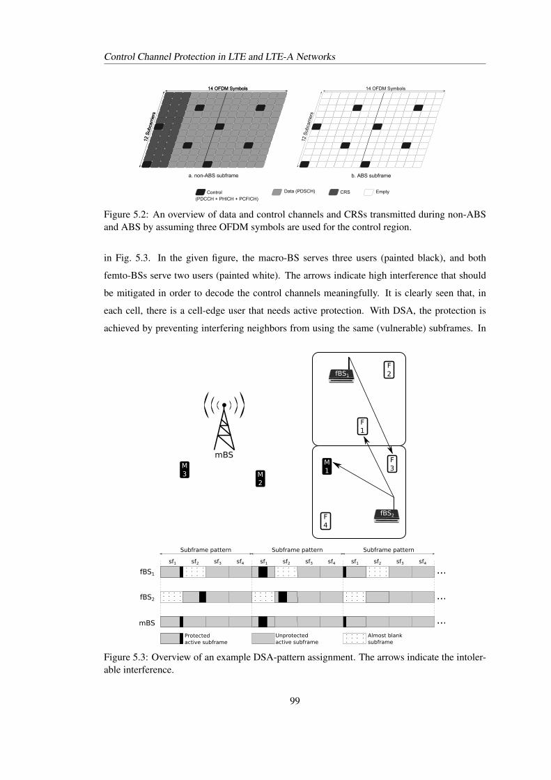
Control Channel Protection in LTE and LTE-A Networks
14HOFDMHSymbols
12HS
ubca
rrie
rs
14HOFDMHSymbols
12HS
ubca
rrie
rs
a.Hnon-ABSHsubframe b.HABSHsubframe
DataH(PDSCH) CRSControlH(PDCCHH+HPHICHH+HPCFICH)
Empty
14HOFDMHSymbols
12HS
ubca
rrie
rs
Figure 5.2: An overview of data and control channels and CRSs transmitted during non-ABSand ABS by assuming three OFDM symbols are used for the control region.
in Fig. 5.3. In the given figure, the macro-BS serves three users (painted black), and both
femto-BSs serve two users (painted white). The arrows indicate high interference that should
be mitigated in order to decode the control channels meaningfully. It is clearly seen that, in
each cell, there is a cell-edge user that needs active protection. With DSA, the protection is
achieved by preventing interfering neighbors from using the same (vulnerable) subframes. In
M2
M1
F1
F3
fBS1
fBS2
mBSM3
F2
F4
Protected active subframe
Unprotected active subframe
. . . .. . . .
. . . .Almost blank subframe
. . . .. . . .
. . . .. . . .. . . .. . . .
. . . .. . . .
. . . .
. . . .. . . .
. . . .. . . .. . . .. . . .
. . . .. . . .
. . . .
Subframe pattern Subframe pattern Subframe pattern
...
...
...
fBS1
fBS2
mBS
sf1 sf2 sf3 sf4 sf1 sf2 sf3 sf4 sf1 sf2 sf3 sf4
Figure 5.3: Overview of an example DSA-pattern assignment. The arrows indicate the intoler-able interference.
99
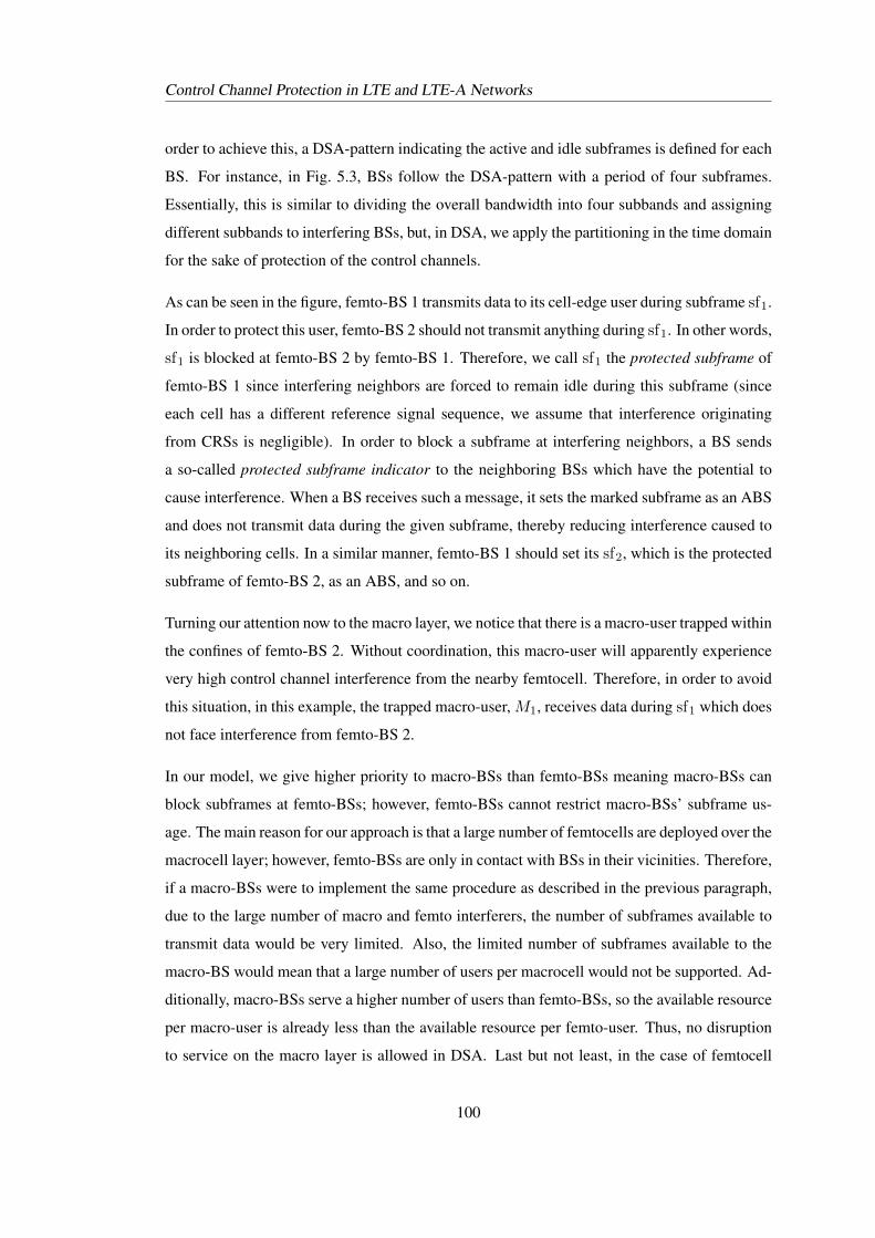
Control Channel Protection in LTE and LTE-A Networks
order to achieve this, a DSA-pattern indicating the active and idle subframes is defined for each
BS. For instance, in Fig. 5.3, BSs follow the DSA-pattern with a period of four subframes.
Essentially, this is similar to dividing the overall bandwidth into four subbands and assigning
different subbands to interfering BSs, but, in DSA, we apply the partitioning in the time domain
for the sake of protection of the control channels.
As can be seen in the figure, femto-BS 1 transmits data to its cell-edge user during subframe sf1.
In order to protect this user, femto-BS 2 should not transmit anything during sf1. In other words,
sf1 is blocked at femto-BS 2 by femto-BS 1. Therefore, we call sf1 the protected subframe of
femto-BS 1 since interfering neighbors are forced to remain idle during this subframe (since
each cell has a different reference signal sequence, we assume that interference originating
from CRSs is negligible). In order to block a subframe at interfering neighbors, a BS sends
a so-called protected subframe indicator to the neighboring BSs which have the potential to
cause interference. When a BS receives such a message, it sets the marked subframe as an ABS
and does not transmit data during the given subframe, thereby reducing interference caused to
its neighboring cells. In a similar manner, femto-BS 1 should set its sf2, which is the protected
subframe of femto-BS 2, as an ABS, and so on.
Turning our attention now to the macro layer, we notice that there is a macro-user trapped within
the confines of femto-BS 2. Without coordination, this macro-user will apparently experience
very high control channel interference from the nearby femtocell. Therefore, in order to avoid
this situation, in this example, the trapped macro-user, M1, receives data during sf1 which does
not face interference from femto-BS 2.
In our model, we give higher priority to macro-BSs than femto-BSs meaning macro-BSs can
block subframes at femto-BSs; however, femto-BSs cannot restrict macro-BSs’ subframe us-
age. The main reason for our approach is that a large number of femtocells are deployed over the
macrocell layer; however, femto-BSs are only in contact with BSs in their vicinities. Therefore,
if a macro-BSs were to implement the same procedure as described in the previous paragraph,
due to the large number of macro and femto interferers, the number of subframes available to
transmit data would be very limited. Also, the limited number of subframes available to the
macro-BS would mean that a large number of users per macrocell would not be supported. Ad-
ditionally, macro-BSs serve a higher number of users than femto-BSs, so the available resource
per macro-user is already less than the available resource per femto-user. Thus, no disruption
to service on the macro layer is allowed in DSA. Last but not least, in the case of femtocell
100
Control Channel Protection in LTE and LTE-A Networks
deployments, indoor macro-users face excessive interference from femto-BSs, whereas due to
the wall penetration loss, interference from macro-BSs to femto-users is not significant. Thus,
femto-users do not suffer significant performance degradation if macro-BSs do not restrict their
subframe assignments.
The remaining subframes which are neither set as protected nor blocked by other BSs, such as
sf3 and sf4 of femto-BS 1, can be used by the femto-BSs for their cell-center users without any
restriction but also without enjoying any protection privileges. Such use of subframes is the
main advantage of the proposed DSA method where BSs can protect their cell-edge users with
the protected subframes, and they can use further subframes as long as they do not cause high
interference to their neighbors. Such flexibility eventually increases the resource utilization of
the network with respect to the static ABS methods where the ratio of ABS used by femtocells
and macrocells are set a priori.
5.3.1 Required Measurement and Signaling
5.3.1.1 Definition of Interfering BSs
In order to provide a reliable control channel reception, in DSA, a global, pre-defined minimum
SINR threshold, γmin, is used. γmin is the minimum desired SINR for each user for correct de-
coding of the control channels for the downlink transmission. Given the pre-defined minimum
SINR value in a network, DSA provides the γmin condition for each user by preventing the in-
terfering BSs from transmitting a signal over chosen subframes. In this way, we have a system
where all users experience control region SINRs that are high enough for the reliable reception
of the control signals.
In order to allocate resources to its users, a BS needs to fulfill the γmin condition for each user it
is serving. Therefore, the BS should know interfering BSs from which it protects its users. This
is not straightforward in femtocell networks as they are deployed randomly by end users where
the number and the positions of femtocells may vary during the operation of the network. Since
the locations of neighboring BSs cannot be determined a priori, it is impossible for a user to
identify the list of interfering BSs in advance. For this purpose, the serving BS identifies the
interfering BS for its users based on its users’ feedback.
Theoretically, by assuming that all BSs are active during the same subframe, the control region
101
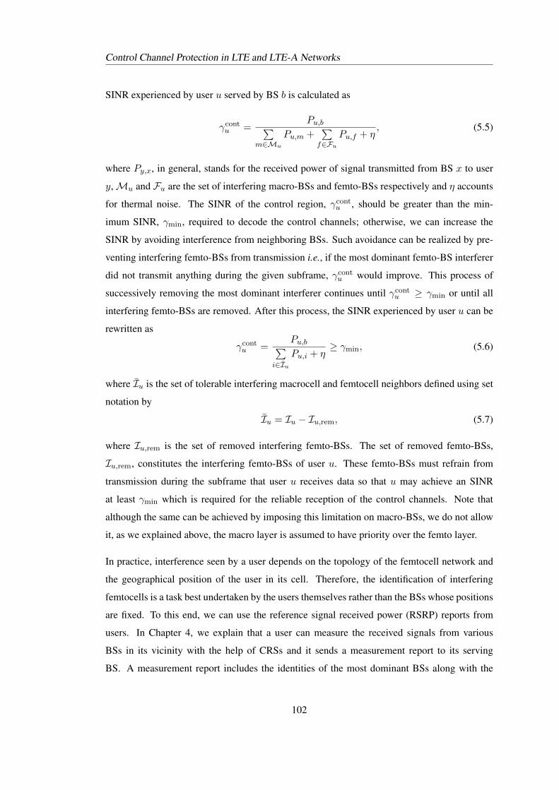
Control Channel Protection in LTE and LTE-A Networks
SINR experienced by user u served by BS b is calculated as
γcontu =
Pu,b∑m∈Mu
Pu,m +∑f∈Fu
Pu,f + η, (5.5)
where Py,x, in general, stands for the received power of signal transmitted from BS x to user
y,Mu and Fu are the set of interfering macro-BSs and femto-BSs respectively and η accounts
for thermal noise. The SINR of the control region, γcontu , should be greater than the min-
imum SINR, γmin, required to decode the control channels; otherwise, we can increase the
SINR by avoiding interference from neighboring BSs. Such avoidance can be realized by pre-
venting interfering femto-BSs from transmission i.e., if the most dominant femto-BS interferer
did not transmit anything during the given subframe, γcontu would improve. This process of
successively removing the most dominant interferer continues until γcontu ≥ γmin or until all
interfering femto-BSs are removed. After this process, the SINR experienced by user u can be
rewritten as
γcontu =
Pu,b∑i∈Iu
Pu,i + η≥ γmin, (5.6)
where Iu is the set of tolerable interfering macrocell and femtocell neighbors defined using set
notation by
Iu = Iu − Iu,rem, (5.7)
where Iu,rem is the set of removed interfering femto-BSs. The set of removed femto-BSs,
Iu,rem, constitutes the interfering femto-BSs of user u. These femto-BSs must refrain from
transmission during the subframe that user u receives data so that u may achieve an SINR
at least γmin which is required for the reliable reception of the control channels. Note that
although the same can be achieved by imposing this limitation on macro-BSs, we do not allow
it, as we explained above, the macro layer is assumed to have priority over the femto layer.
In practice, interference seen by a user depends on the topology of the femtocell network and
the geographical position of the user in its cell. Therefore, the identification of interfering
femtocells is a task best undertaken by the users themselves rather than the BSs whose positions
are fixed. To this end, we can use the reference signal received power (RSRP) reports from
users. In Chapter 4, we explain that a user can measure the received signals from various
BSs in its vicinity with the help of CRSs and it sends a measurement report to its serving
BS. A measurement report includes the identities of the most dominant BSs along with the
102
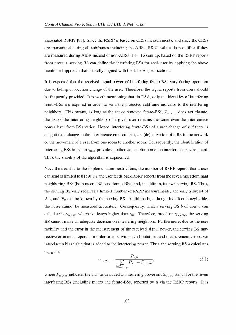
Control Channel Protection in LTE and LTE-A Networks
associated RSRPs [88]. Since the RSRP is based on CRSs measurements, and since the CRSs
are transmitted during all subframes including the ABSs, RSRP values do not differ if they
are measured during ABSs instead of non-ABSs [14]. To sum up, based on the RSRP reports
from users, a serving BS can define the interfering BSs for each user by applying the above
mentioned approach that is totally aligned with the LTE-A specifications.
It is expected that the received signal power of interfering femto-BSs vary during operation
due to fading or location change of the user. Therefore, the signal reports from users should
be frequently provided. It is worth mentioning that, in DSA, only the identities of interfering
femto-BSs are required in order to send the protected subframe indicator to the interfering
neighbors. This means, as long as the set of removed femto-BSs, Iu,rem, does not change,
the list of the interfering neighbors of a given user remains the same even the interference
power level from BSs varies. Hence, interfering femto-BSs of a user change only if there is
a significant change in the interference environment, i.e. (de)activation of a BS in the network
or the movement of a user from one room to another room. Consequently, the identification of
interfering BSs based on γmin provides a rather static definition of an interference environment.
Thus, the stability of the algorithm is augmented.
Nevertheless, due to the implementation restrictions, the number of RSRP reports that a user
can send is limited to 8 [89], i.e. the user feeds back RSRP reports from the seven most dominant
neighboring BSs (both macro-BSs and femto-BSs) and, in addition, its own serving BS. Thus,
the serving BS only receives a limited number of RSRP measurements, and only a subset of
Mu and Fu can be known by the serving BS. Additionally, although its effect is negligible,
the noise cannot be measured accurately. Consequently, what a serving BS b of user u can
calculate is γu,calc which is always higher than γu. Therefore, based on γu,calc, the serving
BS cannot make an adequate decision on interfering neighbors. Furthermore, due to the user
mobility and the error in the measurement of the received signal power, the serving BS may
receive erroneous reports. In order to cope with such limitations and measurement errors, we
introduce a bias value that is added to the interfering power. Thus, the serving BS b calculates
γu,calc as
γu,calc =Pu,b∑
i∈Iu,repPu,i + Pu,bias
, (5.8)
where Pu,bias indicates the bias value added as interfering power and Iu,rep stands for the seven
interfering BSs (including macro and femto-BSs) reported by u via the RSRP reports. It is
103
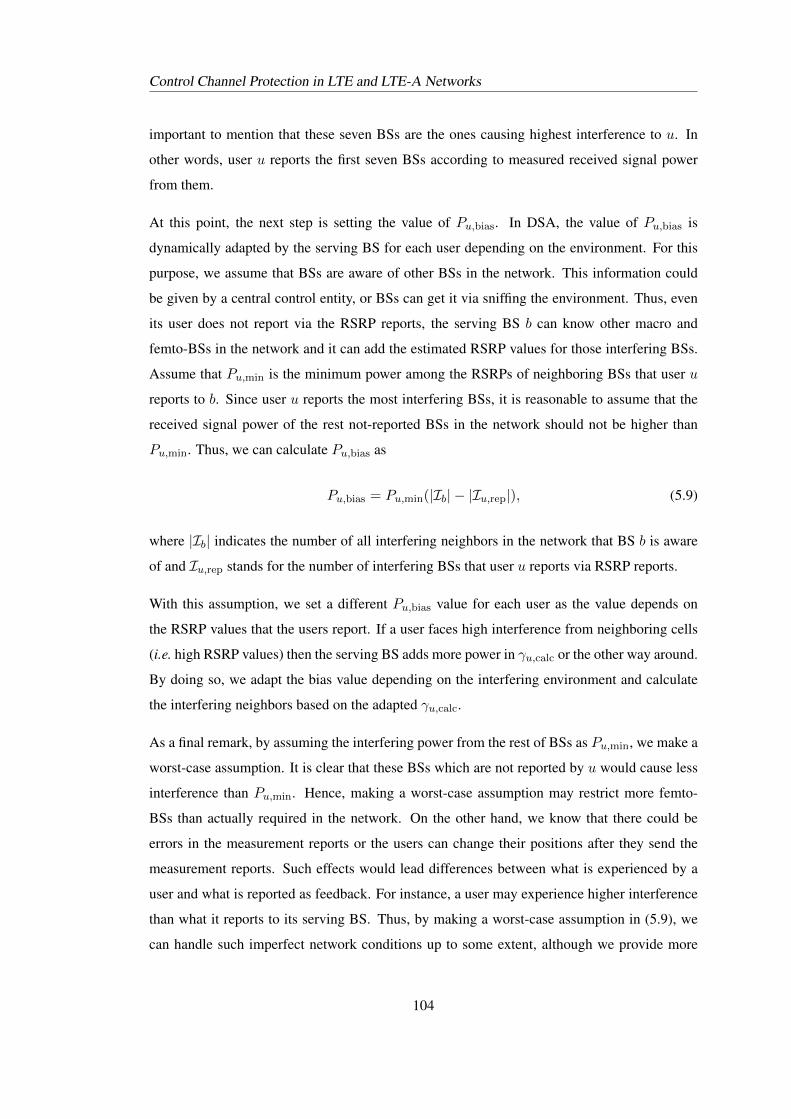
Control Channel Protection in LTE and LTE-A Networks
important to mention that these seven BSs are the ones causing highest interference to u. In
other words, user u reports the first seven BSs according to measured received signal power
from them.
At this point, the next step is setting the value of Pu,bias. In DSA, the value of Pu,bias is
dynamically adapted by the serving BS for each user depending on the environment. For this
purpose, we assume that BSs are aware of other BSs in the network. This information could
be given by a central control entity, or BSs can get it via sniffing the environment. Thus, even
its user does not report via the RSRP reports, the serving BS b can know other macro and
femto-BSs in the network and it can add the estimated RSRP values for those interfering BSs.
Assume that Pu,min is the minimum power among the RSRPs of neighboring BSs that user u
reports to b. Since user u reports the most interfering BSs, it is reasonable to assume that the
received signal power of the rest not-reported BSs in the network should not be higher than
Pu,min. Thus, we can calculate Pu,bias as
Pu,bias = Pu,min(|Ib| − |Iu,rep|), (5.9)
where |Ib| indicates the number of all interfering neighbors in the network that BS b is aware
of and Iu,rep stands for the number of interfering BSs that user u reports via RSRP reports.
With this assumption, we set a different Pu,bias value for each user as the value depends on
the RSRP values that the users report. If a user faces high interference from neighboring cells
(i.e. high RSRP values) then the serving BS adds more power in γu,calc or the other way around.
By doing so, we adapt the bias value depending on the interfering environment and calculate
the interfering neighbors based on the adapted γu,calc.
As a final remark, by assuming the interfering power from the rest of BSs as Pu,min, we make a
worst-case assumption. It is clear that these BSs which are not reported by u would cause less
interference than Pu,min. Hence, making a worst-case assumption may restrict more femto-
BSs than actually required in the network. On the other hand, we know that there could be
errors in the measurement reports or the users can change their positions after they send the
measurement reports. Such effects would lead differences between what is experienced by a
user and what is reported as feedback. For instance, a user may experience higher interference
than what it reports to its serving BS. Thus, by making a worst-case assumption in (5.9), we
can handle such imperfect network conditions up to some extent, although we provide more
104
Control Channel Protection in LTE and LTE-A Networks
protection than required.
5.3.1.2 Protecting Cell-Edge Users via Protected Subframe Indicators
Having knowledge of the (sub-optimal) set of interfering femto-BSs, Iu,rem, the serving BS b
can inform the (potential) interfering femto-BSs of user u via a protected subframe indicator.
In this way, BS b prevents those interfering femto-BSs from using the subframe it sets as a
protected subframe and the required control region SINR can be achieved at user u. If a BS
serves multiple users, then it should perform the same process for all users since each user has
a distinct set of interfering femto-BSs depending on its location.
The protected subframe indicator is not explicitly defined in LTE-A, but the exchange of ABS
patterns between BSs with a period of 40 subframes (in FDD) in terms of a bitmap is sup-
ported [14, 67]. It is up to the network provider to decide what a BS should do upon receiving
an ABS pattern from neighboring BSs. At this point, by assuming there is an X2 signaling of
the ABS pattern between femto-BSs and between femto and macro-BSs, we can make use of
this signaling for the purpose of signaling the protected subframe indicator. For this purpose,
we need to define what information a BS should send via an ABS pattern and what a BS should
do when it receives an ABS pattern.
A BS should set its protected subframe as 1 in the ABS pattern to be signaled and send this
information to the neighboring femtocells that are defined according to (5.6). Based on this,
upon receiving the ABS pattern, a receiver femto-BS should set the subframes which are indi-
cated as 1 in the bitmap as an ABS. Thus, without requiring any change in the specifications,
we can implement the protected subframe indicator just by redefining the use of the signaled
ABS patterns. Please note that although the ABS pattern has a length of 40 subframes, in DSA,
we can use subframe patterns smaller than 40. For instance, in the above example illustrated
in Fig. 5.3, BSs apply DSA based on a DSA-pattern having a length of four subframes. In
such a case, when a BS sends an ABS pattern bitmap, it extends the DSA-pattern to 40 sub-
frames by just repeating the DSA-pattern ten times. Fig. 5.4 illustrates the DSA-pattern sent by
femto-BS 1 to femto-BS 2 based on the subframe pattern shown in Fig. 5.3.
105
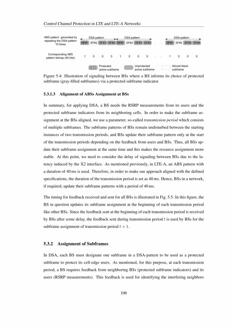
Control Channel Protection in LTE and LTE-A Networks
DSA-pattern
SFv2 SFv3 SFv4SFv1 SFv1 SFv2 SFv3 SFv4
DSA-pattern
SFv1 SFv2 SFv3 SFv4
DSA-pattern
1 0 0 0 1 0 0 0 . . 1 0 0 0
ABS)pattern))generated)by)repeating)the)DSA-pattern
10)times)
Corresponding)ABS)pattern)bitmap)k40)bits))
. .SFv1 SFv1
Protectedactive)subframe
Unprotectedactive)subframe
Almost)blanksubframe
Figure 5.4: Illustration of signaling between BSs where a BS informs its choice of protectedsubframe (gray-filled subframes) via a protected subframe indicator.
5.3.1.3 Alignment of ABSs Assignment at BSs
In summary, for applying DSA, a BS needs the RSRP measurements from its users and the
protected subframe indicators from its neighboring cells. In order to make the subframe as-
signment at the BSs aligned, we use a parameter, so-called transmission period which consists
of multiple subframes. The subframe patterns of BSs remain undisturbed between the starting
instances of two transmission periods, and BSs update their subframe pattern only at the start
of the transmission periods depending on the feedback from users and BSs. Thus, all BSs up-
date their subframe assignment at the same time and this makes the resource assignment more
stable. At this point, we need to consider the delay of signaling between BSs due to the la-
tency induced by the X2 interface. As mentioned previously, in LTE-A, an ABS pattern with
a duration of 40 ms is used. Therefore, in order to make our approach aligned with the defined
specifications, the duration of the transmission period is set as 40 ms. Hence, BSs in a network,
if required, update their subframe patterns with a period of 40 ms.
The timing for feedback received and sent for all BSs is illustrated in Fig. 5.5. In this figure, the
BS in question updates its subframe assignment at the beginning of each transmission period
like other BSs. Since the feedback sent at the beginning of each transmission period is received
by BSs after some delay, the feedback sent during transmission period t is used by BSs for the
subframe assignment of transmission period t+ 1.
5.3.2 Assignment of Subframes
In DSA, each BS must designate one subframe in a DSA-pattern to be used as a protected
subframe to protect its cell-edge users. As mentioned, for this purpose, at each transmission
period, a BS requires feedback from neighboring BSs (protected subframe indicators) and its
users (RSRP measurements). This feedback is used for identifying the interfering neighbors
106
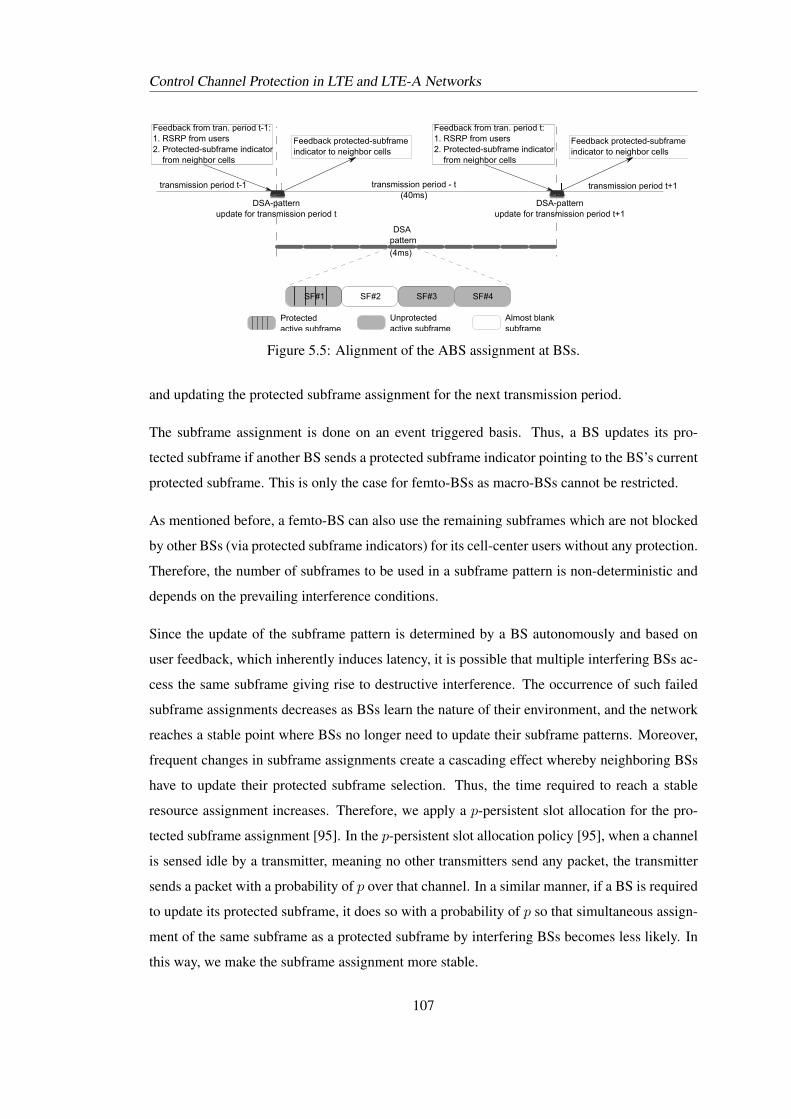
Control Channel Protection in LTE and LTE-A Networks
transmissionhperiodh-htU40ms)h
transmissionhperiodht-1
Feedbackhfromhtran.hperiodht-1:1.hRSRPhfromhusers2.hProtected-subframehindicatorhhhhhfromhneighborhcells
DSAhpattern
U4ms)h
SFA2 SFA3 SFA4
Feedbackhprotected-subframehindicatorhtohneighborhcells
DSA-patternupdatehforhtransmissionhperiodht
DSA-patternupdatehforhtransmissionhperiodht+1
transmissionhperiodht+1
Feedbackhfromhtran.hperiodht:1.hRSRPhfromhusers2.hProtected-subframehindicatorhhhhhfromhneighborhcells
Feedbackhprotected-subframehindicatorhtohneighborhcells
SFA1
Protectedactivehsubframe
Unprotectedactivehsubframe
Almosthblanksubframe
Figure 5.5: Alignment of the ABS assignment at BSs.
and updating the protected subframe assignment for the next transmission period.
The subframe assignment is done on an event triggered basis. Thus, a BS updates its pro-
tected subframe if another BS sends a protected subframe indicator pointing to the BS’s current
protected subframe. This is only the case for femto-BSs as macro-BSs cannot be restricted.
As mentioned before, a femto-BS can also use the remaining subframes which are not blocked
by other BSs (via protected subframe indicators) for its cell-center users without any protection.
Therefore, the number of subframes to be used in a subframe pattern is non-deterministic and
depends on the prevailing interference conditions.
Since the update of the subframe pattern is determined by a BS autonomously and based on
user feedback, which inherently induces latency, it is possible that multiple interfering BSs ac-
cess the same subframe giving rise to destructive interference. The occurrence of such failed
subframe assignments decreases as BSs learn the nature of their environment, and the network
reaches a stable point where BSs no longer need to update their subframe patterns. Moreover,
frequent changes in subframe assignments create a cascading effect whereby neighboring BSs
have to update their protected subframe selection. Thus, the time required to reach a stable
resource assignment increases. Therefore, we apply a p-persistent slot allocation for the pro-
tected subframe assignment [95]. In the p-persistent slot allocation policy [95], when a channel
is sensed idle by a transmitter, meaning no other transmitters send any packet, the transmitter
sends a packet with a probability of p over that channel. In a similar manner, if a BS is required
to update its protected subframe, it does so with a probability of p so that simultaneous assign-
ment of the same subframe as a protected subframe by interfering BSs becomes less likely. In
this way, we make the subframe assignment more stable.
107
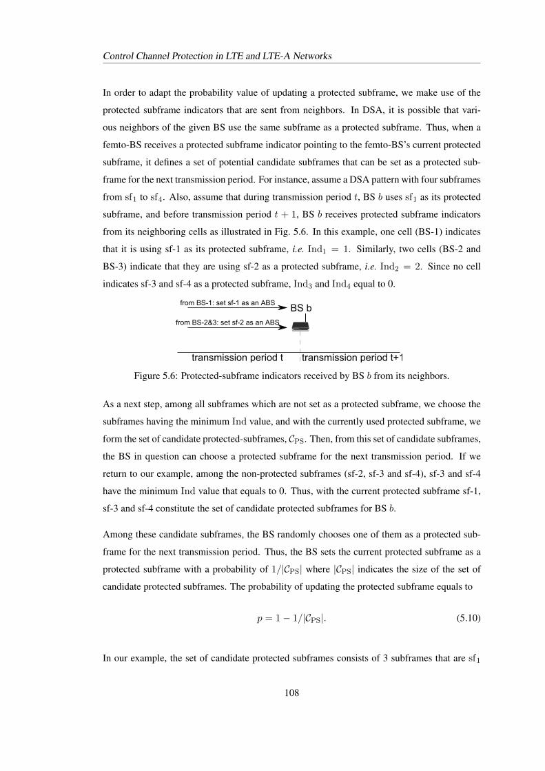
Control Channel Protection in LTE and LTE-A Networks
In order to adapt the probability value of updating a protected subframe, we make use of the
protected subframe indicators that are sent from neighbors. In DSA, it is possible that vari-
ous neighbors of the given BS use the same subframe as a protected subframe. Thus, when a
femto-BS receives a protected subframe indicator pointing to the femto-BS’s current protected
subframe, it defines a set of potential candidate subframes that can be set as a protected sub-
frame for the next transmission period. For instance, assume a DSA pattern with four subframes
from sf1 to sf4. Also, assume that during transmission period t, BS b uses sf1 as its protected
subframe, and before transmission period t + 1, BS b receives protected subframe indicators
from its neighboring cells as illustrated in Fig. 5.6. In this example, one cell (BS-1) indicates
that it is using sf-1 as its protected subframe, i.e. Ind1 = 1. Similarly, two cells (BS-2 and
BS-3) indicate that they are using sf-2 as a protected subframe, i.e. Ind2 = 2. Since no cell
indicates sf-3 and sf-4 as a protected subframe, Ind3 and Ind4 equal to 0.
transmission period t
BS bfrom BS-1: set sf-1 as an ABS
transmission period t+1
from BS-2&3: set sf-2 as an ABS
Figure 5.6: Protected-subframe indicators received by BS b from its neighbors.
As a next step, among all subframes which are not set as a protected subframe, we choose the
subframes having the minimum Ind value, and with the currently used protected subframe, we
form the set of candidate protected-subframes, CPS. Then, from this set of candidate subframes,
the BS in question can choose a protected subframe for the next transmission period. If we
return to our example, among the non-protected subframes (sf-2, sf-3 and sf-4), sf-3 and sf-4
have the minimum Ind value that equals to 0. Thus, with the current protected subframe sf-1,
sf-3 and sf-4 constitute the set of candidate protected subframes for BS b.
Among these candidate subframes, the BS randomly chooses one of them as a protected sub-
frame for the next transmission period. Thus, the BS sets the current protected subframe as a
protected subframe with a probability of 1/|CPS| where |CPS| indicates the size of the set of
candidate protected subframes. The probability of updating the protected subframe equals to
p = 1− 1/|CPS|. (5.10)
In our example, the set of candidate protected subframes consists of 3 subframes that are sf1
108
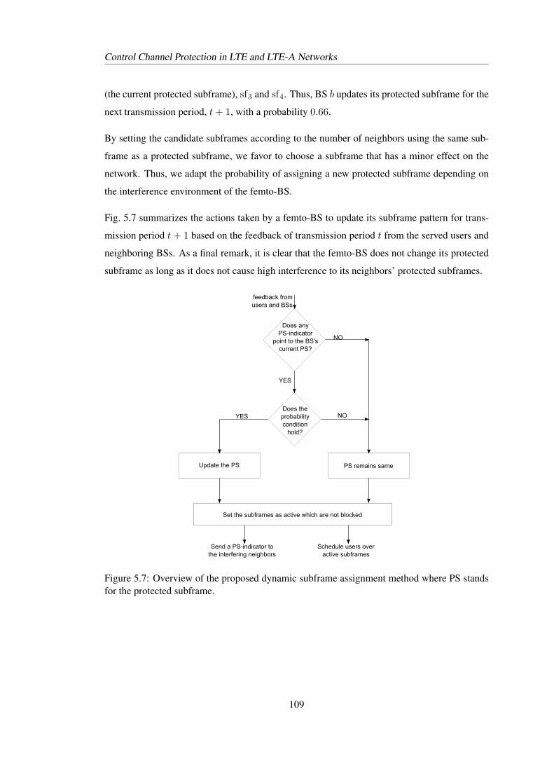
Control Channel Protection in LTE and LTE-A Networks
(the current protected subframe), sf3 and sf4. Thus, BS b updates its protected subframe for the
next transmission period, t+ 1, with a probability 0.66.
By setting the candidate subframes according to the number of neighbors using the same sub-
frame as a protected subframe, we favor to choose a subframe that has a minor effect on the
network. Thus, we adapt the probability of assigning a new protected subframe depending on
the interference environment of the femto-BS.
Fig. 5.7 summarizes the actions taken by a femto-BS to update its subframe pattern for trans-
mission period t+ 1 based on the feedback of transmission period t from the served users and
neighboring BSs. As a final remark, it is clear that the femto-BS does not change its protected
subframe as long as it does not cause high interference to its neighbors’ protected subframes.
PSDremainsDsame
SetDtheDsubframesDasDactiveDwhichDareDnotDblocked
UpdateDtheDPSD
NOYES
SendDaDPS-indicatorDtoDtheDinterferingDneighbors
feedbackDfromDusersDandDBSs
DoesDanyDPS-indicatorD
pointDtoDtheDBS'sDcurrentDPS?
DoesDtheDprobabilityDconditionD
hold?
ScheduleDusersDoverDactiveDsubframes
NO
YES
Figure 5.7: Overview of the proposed dynamic subframe assignment method where PS standsfor the protected subframe.
109
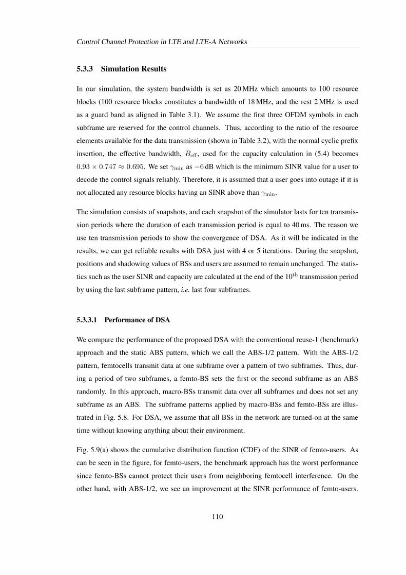
Control Channel Protection in LTE and LTE-A Networks
5.3.3 Simulation Results
In our simulation, the system bandwidth is set as 20 MHz which amounts to 100 resource
blocks (100 resource blocks constitutes a bandwidth of 18 MHz, and the rest 2 MHz is used
as a guard band as aligned in Table 3.1). We assume the first three OFDM symbols in each
subframe are reserved for the control channels. Thus, according to the ratio of the resource
elements available for the data transmission (shown in Table 3.2), with the normal cyclic prefix
insertion, the effective bandwidth, Beff , used for the capacity calculation in (5.4) becomes
0.93 × 0.747 ≈ 0.695. We set γmin as −6 dB which is the minimum SINR value for a user to
decode the control signals reliably. Therefore, it is assumed that a user goes into outage if it is
not allocated any resource blocks having an SINR above than γmin.
The simulation consists of snapshots, and each snapshot of the simulator lasts for ten transmis-
sion periods where the duration of each transmission period is equal to 40 ms. The reason we
use ten transmission periods to show the convergence of DSA. As it will be indicated in the
results, we can get reliable results with DSA just with 4 or 5 iterations. During the snapshot,
positions and shadowing values of BSs and users are assumed to remain unchanged. The statis-
tics such as the user SINR and capacity are calculated at the end of the 10th transmission period
by using the last subframe pattern, i.e. last four subframes.
5.3.3.1 Performance of DSA
We compare the performance of the proposed DSA with the conventional reuse-1 (benchmark)
approach and the static ABS pattern, which we call the ABS-1/2 pattern. With the ABS-1/2
pattern, femtocells transmit data at one subframe over a pattern of two subframes. Thus, dur-
ing a period of two subframes, a femto-BS sets the first or the second subframe as an ABS
randomly. In this approach, macro-BSs transmit data over all subframes and does not set any
subframe as an ABS. The subframe patterns applied by macro-BSs and femto-BSs are illus-
trated in Fig. 5.8. For DSA, we assume that all BSs in the network are turned-on at the same
time without knowing anything about their environment.
Fig. 5.9(a) shows the cumulative distribution function (CDF) of the SINR of femto-users. As
can be seen in the figure, for femto-users, the benchmark approach has the worst performance
since femto-BSs cannot protect their users from neighboring femtocell interference. On the
other hand, with ABS-1/2, we see an improvement at the SINR performance of femto-users.
110
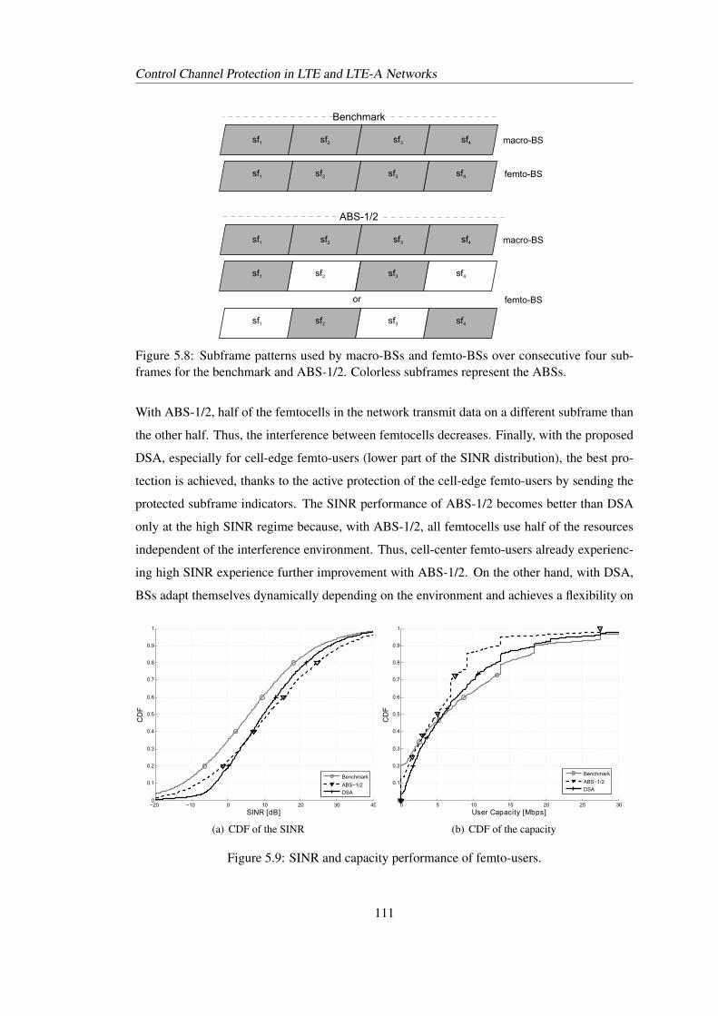
Control Channel Protection in LTE and LTE-A Networks
macro-BS
femto-BS
sf1
sf1
sf2
sf2
sf3
sf3
sf4
sf4
Benchmark
macro-BSsf1 sf2 sf3 sf4
ABS-1/2
femto-BS
sf1 sf2 sf3 sf4
sf1 sf2 sf3 sf4
or
Figure 5.8: Subframe patterns used by macro-BSs and femto-BSs over consecutive four sub-frames for the benchmark and ABS-1/2. Colorless subframes represent the ABSs.
With ABS-1/2, half of the femtocells in the network transmit data on a different subframe than
the other half. Thus, the interference between femtocells decreases. Finally, with the proposed
DSA, especially for cell-edge femto-users (lower part of the SINR distribution), the best pro-
tection is achieved, thanks to the active protection of the cell-edge femto-users by sending the
protected subframe indicators. The SINR performance of ABS-1/2 becomes better than DSA
only at the high SINR regime because, with ABS-1/2, all femtocells use half of the resources
independent of the interference environment. Thus, cell-center femto-users already experienc-
ing high SINR experience further improvement with ABS-1/2. On the other hand, with DSA,
BSs adapt themselves dynamically depending on the environment and achieves a flexibility on
−20 −10 0 10 20 30 400
0.1
0.2
0.3
0.4
0.5
0.6
0.7
0.8
0.9
1
SINRA[dB]
CD
F
Benchmark
ABS−1/2
DSA
(a) CDF of the SINR
0 5 10 15 20 25 300
0.1
0.2
0.3
0.4
0.5
0.6
0.7
0.8
0.9
1
UserhCapacityh[Mbps]
CD
F
Benchmark
ABS−1/2
DSA
(b) CDF of the capacity
Figure 5.9: SINR and capacity performance of femto-users.
111
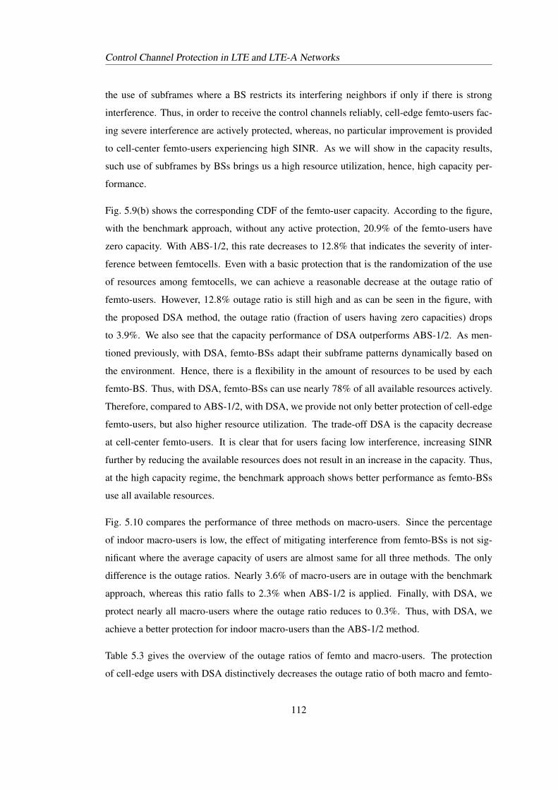
Control Channel Protection in LTE and LTE-A Networks
the use of subframes where a BS restricts its interfering neighbors if only if there is strong
interference. Thus, in order to receive the control channels reliably, cell-edge femto-users fac-
ing severe interference are actively protected, whereas, no particular improvement is provided
to cell-center femto-users experiencing high SINR. As we will show in the capacity results,
such use of subframes by BSs brings us a high resource utilization, hence, high capacity per-
formance.
Fig. 5.9(b) shows the corresponding CDF of the femto-user capacity. According to the figure,
with the benchmark approach, without any active protection, 20.9% of the femto-users have
zero capacity. With ABS-1/2, this rate decreases to 12.8% that indicates the severity of inter-
ference between femtocells. Even with a basic protection that is the randomization of the use
of resources among femtocells, we can achieve a reasonable decrease at the outage ratio of
femto-users. However, 12.8% outage ratio is still high and as can be seen in the figure, with
the proposed DSA method, the outage ratio (fraction of users having zero capacities) drops
to 3.9%. We also see that the capacity performance of DSA outperforms ABS-1/2. As men-
tioned previously, with DSA, femto-BSs adapt their subframe patterns dynamically based on
the environment. Hence, there is a flexibility in the amount of resources to be used by each
femto-BS. Thus, with DSA, femto-BSs can use nearly 78% of all available resources actively.
Therefore, compared to ABS-1/2, with DSA, we provide not only better protection of cell-edge
femto-users, but also higher resource utilization. The trade-off DSA is the capacity decrease
at cell-center femto-users. It is clear that for users facing low interference, increasing SINR
further by reducing the available resources does not result in an increase in the capacity. Thus,
at the high capacity regime, the benchmark approach shows better performance as femto-BSs
use all available resources.
Fig. 5.10 compares the performance of three methods on macro-users. Since the percentage
of indoor macro-users is low, the effect of mitigating interference from femto-BSs is not sig-
nificant where the average capacity of users are almost same for all three methods. The only
difference is the outage ratios. Nearly 3.6% of macro-users are in outage with the benchmark
approach, whereas this ratio falls to 2.3% when ABS-1/2 is applied. Finally, with DSA, we
protect nearly all macro-users where the outage ratio reduces to 0.3%. Thus, with DSA, we
achieve a better protection for indoor macro-users than the ABS-1/2 method.
Table 5.3 gives the overview of the outage ratios of femto and macro-users. The protection
of cell-edge users with DSA distinctively decreases the outage ratio of both macro and femto-
112
Control Channel Protection in LTE and LTE-A Networks
−10 −5 0 5 10 15 200
0.1
0.2
0.3
0.4
0.5
0.6
0.7
0.8
0.9
1
SINRA[dB]
CD
F
Benchmark
ABS−1/2
DSA
(a) CDF of the SINR
0 0.5 1 1.5 2 2.5 3 3.5 4 4.5 50
0.1
0.2
0.3
0.4
0.5
0.6
0.7
0.8
0.9
1
UserhCapacityh[Mbps]
CD
F
Benchmark
ABS−1/2
DSA
(b) CDF of the capacity
Figure 5.10: SINR and capacity performance of macro-users.
users. Unlike other methods, with DSA, BSs actively play a role in the subframe assignment
depending on the interference conditions. With DSA, compared to the benchmark approach,
the reduction in the outage ratios of femto and macro-users is more than 80% and 90%, respec-
tively. On the other hand, the reduction in the average femto-user capacity is less than 10%. In
summary, we can conclude that DSA improves the coverage of macro and femto-BSs without
causing a dramatic decrease in the overall system capacity.
macro-user femto-user macro-user femto-userMethod Outage Ratio Outage Ratio Avg. User Cap. Avg. User Cap.
[%] [%] [Mbps] [Mbps]
Benchmark 3.6 20.9 1.77 8.95
ABS-1/2 2.3 12.8 1.78 5.88
DSA 0.3 3.9 1.78 8.14
Table 5.3: Outage ratios and average capacities of macro and femto-users.
5.3.3.2 Signaling Overhead
We show that with DSA, we efficiently protect cell-edge users. However, the trade-off DSA is
the signaling overhead because in order to implement DSA, we need the RSRP reports from
users and the protected subframe indicators from neighboring BSs.
As explained in Chapter 4, RSRP values are mapped onto integer values from 0 to 97. Thus,
we can make a simple assumption and set each RSRP report overhead as 7 bits. Also, we
113
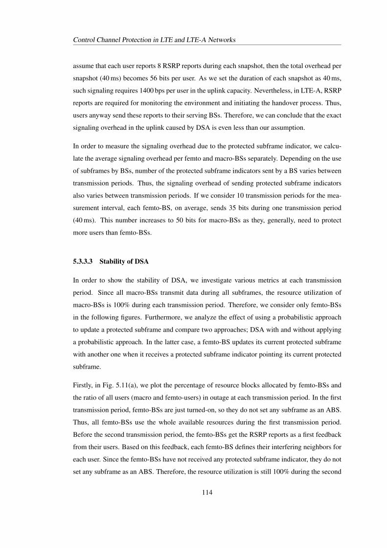
Control Channel Protection in LTE and LTE-A Networks
assume that each user reports 8 RSRP reports during each snapshot, then the total overhead per
snapshot (40 ms) becomes 56 bits per user. As we set the duration of each snapshot as 40 ms,
such signaling requires 1400 bps per user in the uplink capacity. Nevertheless, in LTE-A, RSRP
reports are required for monitoring the environment and initiating the handover process. Thus,
users anyway send these reports to their serving BSs. Therefore, we can conclude that the exact
signaling overhead in the uplink caused by DSA is even less than our assumption.
In order to measure the signaling overhead due to the protected subframe indicator, we calcu-
late the average signaling overhead per femto and macro-BSs separately. Depending on the use
of subframes by BSs, number of the protected subframe indicators sent by a BS varies between
transmission periods. Thus, the signaling overhead of sending protected subframe indicators
also varies between transmission periods. If we consider 10 transmission periods for the mea-
surement interval, each femto-BS, on average, sends 35 bits during one transmission period
(40 ms). This number increases to 50 bits for macro-BSs as they, generally, need to protect
more users than femto-BSs.
5.3.3.3 Stability of DSA
In order to show the stability of DSA, we investigate various metrics at each transmission
period. Since all macro-BSs transmit data during all subframes, the resource utilization of
macro-BSs is 100% during each transmission period. Therefore, we consider only femto-BSs
in the following figures. Furthermore, we analyze the effect of using a probabilistic approach
to update a protected subframe and compare two approaches; DSA with and without applying
a probabilistic approach. In the latter case, a femto-BS updates its current protected subframe
with another one when it receives a protected subframe indicator pointing its current protected
subframe.
Firstly, in Fig. 5.11(a), we plot the percentage of resource blocks allocated by femto-BSs and
the ratio of all users (macro and femto-users) in outage at each transmission period. In the first
transmission period, femto-BSs are just turned-on, so they do not set any subframe as an ABS.
Thus, all femto-BSs use the whole available resources during the first transmission period.
Before the second transmission period, the femto-BSs get the RSRP reports as a first feedback
from their users. Based on this feedback, each femto-BS defines their interfering neighbors for
each user. Since the femto-BSs have not received any protected subframe indicator, they do not
set any subframe as an ABS. Therefore, the resource utilization is still 100% during the second
114
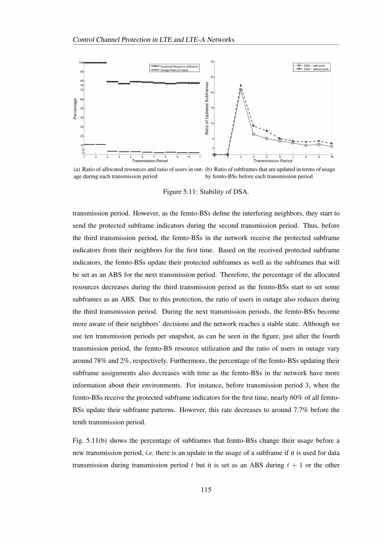
Control Channel Protection in LTE and LTE-A Networks
1 2 3 4 5 6 7 8 9 10 11
25
10
20
30
40
50
60
70
75
80
90
100
TransmissionOPeriod
Per
cen
tag
e
Femtocell Resource UtilizationOutage Ratio of Users
(a) Ratio of allocated resources and ratio of users in out-age during each transmission period
1 2 3 4 5 6 7 8 9 1010
2
5
10
15
20
25
30
TransmissionAPeriod
Rat
ioAo
fAU
pd
ated
ASu
bfr
ames
DSAA−AwithAprob.DSAA−AwithoutAprob.
(b) Ratio of subframes that are updated in terms of usageby femto-BSs before each transmission period
Figure 5.11: Stability of DSA.
transmission period. However, as the femto-BSs define the interfering neighbors, they start to
send the protected subframe indicators during the second transmission period. Thus, before
the third transmission period, the femto-BSs in the network receive the protected subframe
indicators from their neighbors for the first time. Based on the received protected subframe
indicators, the femto-BSs update their protected subframes as well as the subframes that will
be set as an ABS for the next transmission period. Therefore, the percentage of the allocated
resources decreases during the third transmission period as the femto-BSs start to set some
subframes as an ABS. Due to this protection, the ratio of users in outage also reduces during
the third transmission period. During the next transmission periods, the femto-BSs become
more aware of their neighbors’ decisions and the network reaches a stable state. Although we
use ten transmission periods per snapshot, as can be seen in the figure, just after the fourth
transmission period, the femto-BS resource utilization and the ratio of users in outage vary
around 78% and 2%, respectively. Furthermore, the percentage of the femto-BSs updating their
subframe assignments also decreases with time as the femto-BSs in the network have more
information about their environments. For instance, before transmission period 3, when the
femto-BSs receive the protected subframe indicators for the first time, nearly 60% of all femto-
BSs update their subframe patterns. However, this rate decreases to around 7.7% before the
tenth transmission period.
Fig. 5.11(b) shows the percentage of subframes that femto-BSs change their usage before a
new transmission period, i.e. there is an update in the usage of a subframe if it is used for data
transmission during transmission period t but it is set as an ABS during t + 1 or the other
115
Control Channel Protection in LTE and LTE-A Networks
way around. Thus, the ratio of subframes of which usages are updated between transmission
periods t and t + 1 are calculated as N+SF+N−
SFNSF
where NSF is the total number of subframes in
the subframe pattern, N+SF is the number of subframes that remain idle (set as an ABS) during
transmission period t but will be active during t + 1 and N−SF is the number of subframes
that a femto-BS transmits data during transmission period t but sets as an ABS during t + 1.
According to Fig. 5.11(b), since the femto-BSs actively use all subframes in the subframe
pattern, there is no change in the use of subframes during transmission periods 1 and 2. By
receiving the protected subframe indicators, nearly 20% of all subframes are set as an ABS
and remain idle during the third transmission period. Afterwards, as the femto-BSs get more
feedback, the number of subframes that are updated by the femto-BSs decreases. As can be
seen in the figure, only after the fifth transmission period, the femto-BSs change the use of
less than 5% of all subframes. Thus, it can be concluded that with the proposed DSA method,
femto-BSs in a network reach to a stable resource assignment just after couple of iterations
which is a crucial property for a distributed approach. Furthermore, if we apply DSA without
using any probabilistic approach, we see that the number of subframes updated by femto-BSs
before each transmission period increases. For instance, before transmission period 4, around
6.6% of all subframes are updated by femto-BSs with DSA, whereas this rate increases to 9.3%
when no probability condition is applied. This is a more than 40% increase in the ratio of the
updated subframes compared to DSA. These results indicate the effectiveness of the use of a
probabilistic approach when a femto-BS updates its protected subframe.
It is important to mention that we assume the worst-case scenario where BSs are turned on
at the same time without knowing any information about their environment. If a BS enters a
network where other BSs are active, it can reach the stable resource assignment even quicker as
its neighbors already know their interfering environment. As a final remark, BSs in a network
competes for all resources that are available for them. If we introduce traffic conditions, BS
would not use more resources than they require, so total interference in the network decreases
and the stability in the resource assignment is improved.
5.4 Protection of Cell-Edge Users via Cross-Carrier Scheduling
In the previous section, we show how we can dynamically protect the control channels of users
in the time domain with the help of the ABS technique. In this section, we present another
method where we can achieve a control region protection in the frequency domain where the
116
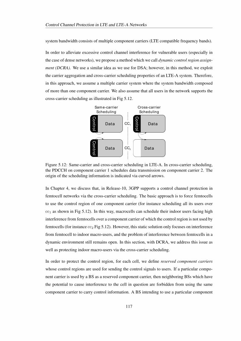
Control Channel Protection in LTE and LTE-A Networks
system bandwidth consists of multiple component carriers (LTE compatible frequency bands).
In order to alleviate excessive control channel interference for vulnerable users (especially in
the case of dense networks), we propose a method which we call dynamic control region assign-
ment (DCRA). We use a similar idea as we use for DSA; however, in this method, we exploit
the carrier aggregation and cross-carrier scheduling properties of an LTE-A system. Therefore,
in this approach, we assume a multiple carrier system where the system bandwidth composed
of more than one component carrier. We also assume that all users in the network supports the
cross-carrier scheduling as illustrated in Fig 5.12.
CC1
CC2Control
Data
Control
Data
Control
Data
Data
Same-carrierScheduling
Cross-carrierScheduling
Figure 5.12: Same-carrier and cross-carrier scheduling in LTE-A. In cross-carrier scheduling,the PDCCH on component carrier 1 schedules data transmission on component carrier 2. Theorigin of the scheduling information is indicated via curved arrows.
In Chapter 4, we discuss that, in Release-10, 3GPP supports a control channel protection in
femtocell networks via the cross-carrier scheduling. The basic approach is to force femtocells
to use the control region of one component carrier (for instance scheduling all its users over
cc1 as shown in Fig 5.12). In this way, macrocells can schedule their indoor users facing high
interference from femtocells over a component carrier of which the control region is not used by
femtocells (for instance cc2 Fig 5.12). However, this static solution only focuses on interference
from femtocell to indoor macro-users, and the problem of interference between femtocells in a
dynamic environment still remains open. In this section, with DCRA, we address this issue as
well as protecting indoor macro-users via the cross-carrier scheduling.
In order to protect the control region, for each cell, we define reserved component carriers
whose control regions are used for sending the control signals to users. If a particular compo-
nent carrier is used by a BS as a reserved component carrier, then neighboring BSs which have
the potential to cause interference to the cell in question are forbidden from using the same
component carrier to carry control information. A BS intending to use a particular component
117
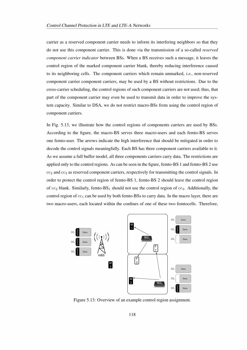
Control Channel Protection in LTE and LTE-A Networks
carrier as a reserved component carrier needs to inform its interfering neighbors so that they
do not use this component carrier. This is done via the transmission of a so-called reserved
component carrier indicator between BSs. When a BS receives such a message, it leaves the
control region of the marked component carrier blank, thereby reducing interference caused
to its neighboring cells. The component carriers which remain unmarked, i.e., non-reserved
component carrier component carriers, may be used by a BS without restrictions. Due to the
cross-carrier scheduling, the control regions of such component carriers are not used; thus, that
part of the component carrier may even be used to transmit data in order to improve the sys-
tem capacity. Similar to DSA, we do not restrict macro-BSs from using the control region of
component carriers.
In Fig. 5.13, we illustrate how the control regions of components carriers are used by BSs.
According to the figure, the macro-BS serves three macro-users and each femto-BS serves
one femto-user. The arrows indicate the high interference that should be mitigated in order to
decode the control signals meaningfully. Each BS has three component carriers available to it.
As we assume a full buffer model, all three components carriers carry data. The restrictions are
applied only to the control regions. As can be seen in the figure, femto-BS 1 and femto-BS 2 use
cc2 and cc3 as reserved component carriers, respectively for transmitting the control signals. In
order to protect the control region of femto-BS 1, femto-BS 2 should leave the control region
of cc2 blank. Similarly, femto-BS1 should not use the control region of cc3. Additionally, the
control region of cc1 can be used by both femto-BSs to carry data. In the macro layer, there are
two macro-users, each located within the confines of one of these two femtocells. Therefore,
Data
Control
Data
Data
CC1
CC2
CC3
Data
Data
Control
Data
CC1
CC2
CC3
Control
Data
Control
Data
CC1
CC2
CC3
Data
M3
M2
M1
F1
F2
fBS1
fBS2
mBS
mBS
Control
Data
Figure 5.13: Overview of an example control region assignment.
118
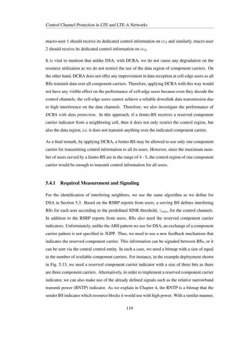
Control Channel Protection in LTE and LTE-A Networks
macro-user 1 should receive its dedicated control information on cc3 and similarly, macro-user
2 should receive its dedicated control information on cc2.
It is vital to mention that unlike DSA, with DCRA, we do not cause any degradation on the
resource utilization as we do not restrict the use of the data region of component carriers. On
the other hand, DCRA does not offer any improvement in data reception at cell-edge users as all
BSs transmit data over all component carriers. Therefore, applying DCRA with this way would
not have any visible effect on the performance of cell-edge users because even they decode the
control channels, the cell-edge users cannot achieve a reliable downlink data transmission due
to high interference on the data channels. Therefore, we also investigate the performance of
DCRA with data protection. In this approach, if a femto-BS receives a reserved component
carrier indicator from a neighboring cell, then it does not only restrict the control region, but
also the data region, i.e. it does not transmit anything over the indicated component carrier.
As a final remark, by applying DCRA, a femto-BS may be allowed to use only one component
carrier for transmitting control information to all its users. However, since the maximum num-
ber of users served by a femto-BS are in the range of 4 - 5, the control region of one component
carrier would be enough to transmit control information for all users.
5.4.1 Required Measurement and Signaling
For the identification of interfering neighbors, we use the same algorithm as we define for
DSA in Section 5.3. Based on the RSRP reports from users, a serving BS defines interfering
BSs for each user according to the predefined SINR threshold, γmin, for the control channels.
In addition to the RSRP reports from users, BSs also need the reserved component carrier
indicators. Unfortunately, unlike the ABS pattern we use for DSA, an exchange of a component
carrier pattern is not specified in 3GPP. Thus, we need to use a new feedback mechanism that
indicates the reserved component carrier. This information can be signaled between BSs, or it
can be sent via the central control entity. In such a case, we need a bitmap with a size of equal
to the number of available component carriers. For instance, in the example deployment shown
in Fig. 5.13, we need a reserved component carrier indicator with a size of three bits as there
are three component carriers. Alternatively, in order to implement a reserved component carrier
indicator, we can also make use of the already defined signals such as the relative narrowband
transmit power (RNTP) indicator. As we explain in Chapter 4, the RNTP is a bitmap that the
sender BS indicates which resource blocks it would use with high power. With a similar manner,
119
Control Channel Protection in LTE and LTE-A Networks
once in a given transmission period, we can assume that each BS in the network uses RNTP
for indicating its reserved component carrier. Thus, although the component carrier pattern is
not defined explicitly in LTE-A, it is not difficult to implement such an indicator as a similar
approach for resource blocks is already specified in LTE-A.
Like in DSA, each BS in the network updates its control region usage at the start of transmission
periods depending on the feedback from users and BSs. In order to set the duration of a trans-
mission period, we consider the signaling latency between BSs assuming they send messages
via the X2 interface and the measurement period required for a user. Thus, the duration of a
transmission period should be at least 20 ms where each BS in the network, if required, updates
its control region assignment with the preset transmission period. Consequently, the timing for
feedback received and sent for all BSs is same as the DSA case as illustrated in Fig. 5.14.
FeedbackLfromLtransmissionLperiodLt:1.LRSRPLfromLusers2.LReserved-componentLcarrierLLLLindicatorLfromLneighborLcells
UpdateLreservedLcomponentLcarrier
LeaveLtheLcontrolLregionLofLcomponentLcarriersLindicatedLbyLneighborsLblankL
FeedbackLreservedLcomponentLcarrierLindicatorLtoLneighborLcells
transmissionLperiodLt transmissionLperiodLt+1
Figure 5.14: Overview of DCRA applied by a femto-BS between transmission periods t andt+ 1.
5.4.2 Assignment of Component Carriers
In DCRA, each BS must designate one component carrier to be used as a reserved component
carrier to carry control information. The reserved component carrier of a femto-BS remains
unchanged as long as another BS does not send a reserved component carrier indicator pointing
to the femto-BS’s current reserved component carrier.
In such a case, similar to DSA, we assign a new reserved component carrier by applying a
p-persistent slot allocation policy [95]. If a femto-BS receives a reserved component carrier
indicator pointing to the femto-BS’s current reserved component carrier, it creates a set of
component carriers that are potential candidates for the reserved component carrier to be used
during the next transmission period. This is the same idea as explained in Section 5.3 for DSA;
120
Control Channel Protection in LTE and LTE-A Networks
the only difference is that instead of subframes, we use component carriers. Then, among the
candidate component carriers, the femto-BS chooses the reserved component carrier randomly
for the next transmission period.
After a BS updates its reserved component carrier; it sends the corresponding indicator to its
interfering BSs. Also, the BS can use the control region of the remaining component carriers
which are not blocked by other BSs. When DCRA with data protection is applied, femto-BSs
do not use the data and control regions of the blocked components carriers. As mentioned
previously, component carriers of macro-BSs cannot be restricted.
5.4.3 Simulation Results
For the simulations, we use the same simulation setup as explained in Section 5.2. However,
the system bandwidth consists of four component carriers each having a bandwidth of 5 MHz.
Thus, the overall bandwidth corresponds to 20 MHz. Each component carrier consists of 25
resource blocks (25 resource blocks constitutes a bandwidth of 4.5 MHz, and the rest 0.5 MHz
is used as a guard band as aligned in Table 3.1). Thus, during each subframe, there are, in total,
100 resource blocks that can be allocated to users. We assume the first three OFDM symbols in
each subframe are reserved for the control channels. Therefore, with the normal cyclic prefix
insertion, Beff in (5.4) becomes 0.93 × 0.737 ≈ 0.685 . Furthermore, we set γmin as −6 dB
and assume that a user goes into outage if its control region SINR is below than γmin.
The simulation consists of snapshots, and each snapshot of the simulator lasts for ten trans-
mission periods where the duration of each transmission period is equal to 20 ms. During the
snapshot, positions and shadowing values of BSs and users are assumed to remain unchanged.
The statistics are calculated at the end of the 10th transmission period.
5.4.3.1 Performance of DCRA
The performance of DCRA is compared to reuse-1 and the static cross-carrier scheduling,
which we call CCS-1/2. Reuse-1 is the benchmark system where all BSs use all component
carriers without any coordination whatsoever. In CCS-1/2, femto-BSs use the control region
of two component carriers out of four and blank out the control regions of the remaining two
component carriers. Each femto-BS randomly chooses the component carrier pairs (cc1 and cc3
or cc2 and cc4) over which it sends control information. The usage of the component carriers
121
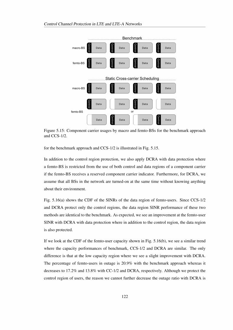
Control Channel Protection in LTE and LTE-A Networks
macro-BS
Co
ntro
l
Data
Co
ntro
l
Data
Co
ntro
l
Data
Co
ntro
l
Data
Co
ntro
l
Data
Co
ntro
l
Data
Co
ntro
l
Data
Co
ntro
l
Datafemto-BS
Benchmark
macro-BS
Co
ntro
l
Data
Co
ntro
l
Data
Co
ntro
l
Data
Co
ntro
l
Data
Co
ntro
l
Data Data
Co
ntro
l
Data Data
femto-BS
Static Cross-carrier Scheduling
DataC
on
trol
Data Data
Co
ntro
l
Data
or
Figure 5.15: Component carrier usages by macro and femto-BSs for the benchmark approachand CCS-1/2.
for the benchmark approach and CCS-1/2 is illustrated in Fig. 5.15.
In addition to the control region protection, we also apply DCRA with data protection where
a femto-BS is restricted from the use of both control and data regions of a component carrier
if the femto-BS receives a reserved component carrier indicator. Furthermore, for DCRA, we
assume that all BSs in the network are turned-on at the same time without knowing anything
about their environment.
Fig. 5.16(a) shows the CDF of the SINRs of the data region of femto-users. Since CCS-1/2
and DCRA protect only the control regions, the data region SINR performance of these two
methods are identical to the benchmark. As expected, we see an improvement at the femto-user
SINR with DCRA with data protection where in addition to the control region, the data region
is also protected.
If we look at the CDF of the femto-user capacity shown in Fig. 5.16(b), we see a similar trend
where the capacity performances of benchmark, CCS-1/2 and DCRA are similar. The only
difference is that at the low capacity region where we see a slight improvement with DCRA.
The percentage of femto-users in outage is 20.9% with the benchmark approach whereas it
decreases to 17.2% and 13.8% with CC-1/2 and DCRA, respectively. Although we protect the
control region of users, the reason we cannot further decrease the outage ratio with DCRA is
122
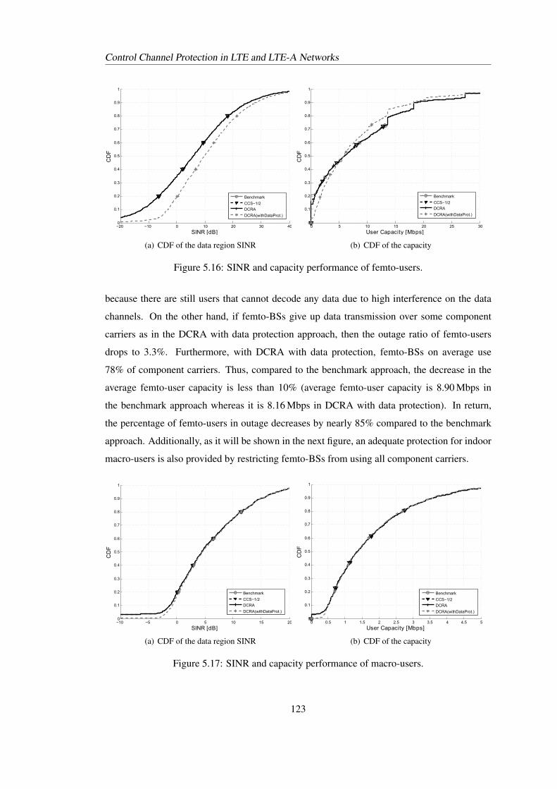
Control Channel Protection in LTE and LTE-A Networks
−20 −10 0 10 20 30 400
0.1
0.2
0.3
0.4
0.5
0.6
0.7
0.8
0.9
1
SINR/[dB]
CD
F
Benchmark
CCS−1/2
DCRA
DCRA)withDataProt.)
(a) CDF of the data region SINR
0 5 10 15 20 25 300
0.1
0.2
0.3
0.4
0.5
0.6
0.7
0.8
0.9
1
UserhCapacityh[Mbps]
CD
F
Benchmark
CCS−1/2
DCRA
DCRAwwithDataProt.P
(b) CDF of the capacity
Figure 5.16: SINR and capacity performance of femto-users.
because there are still users that cannot decode any data due to high interference on the data
channels. On the other hand, if femto-BSs give up data transmission over some component
carriers as in the DCRA with data protection approach, then the outage ratio of femto-users
drops to 3.3%. Furthermore, with DCRA with data protection, femto-BSs on average use
78% of component carriers. Thus, compared to the benchmark approach, the decrease in the
average femto-user capacity is less than 10% (average femto-user capacity is 8.90 Mbps in
the benchmark approach whereas it is 8.16 Mbps in DCRA with data protection). In return,
the percentage of femto-users in outage decreases by nearly 85% compared to the benchmark
approach. Additionally, as it will be shown in the next figure, an adequate protection for indoor
macro-users is also provided by restricting femto-BSs from using all component carriers.
−10 −5 0 5 10 15 200
0.1
0.2
0.3
0.4
0.5
0.6
0.7
0.8
0.9
1
SINR/[dB]
CD
F
Benchmark
CCS−1/2
DCRA
DCRA)withDataProt.)
(a) CDF of the data region SINR
0 0.5 1 1.5 2 2.5 3 3.5 4 4.5 50
0.1
0.2
0.3
0.4
0.5
0.6
0.7
0.8
0.9
1
UserhCapacityh[Mbps]
CD
F
Benchmark
CCS−1/2
DCRA
DCRAwwithDataProt.P
(b) CDF of the capacity
Figure 5.17: SINR and capacity performance of macro-users.
123
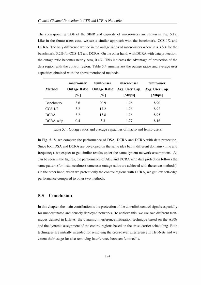
Control Channel Protection in LTE and LTE-A Networks
The corresponding CDF of the SINR and capacity of macro-users are shown in Fig. 5.17.
Like in the femto-users case, we see a similar approach with the benchmark, CCS-1/2 and
DCRA. The only difference we see in the outage ratios of macro-users where it is 3.6% for the
benchmark, 3.2% for CCS-1/2 and DCRA. On the other hand, with DCRA with data protection,
the outage ratio becomes nearly zero, 0.4%. This indicates the advantage of protection of the
data region with the control region. Table 5.4 summarizes the outage ratios and average user
capacities obtained with the above mentioned methods.
macro-user femto-user macro-user femto-userMethod Outage Ratio Outage Ratio Avg. User Cap. Avg. User Cap.
[%] [%] [Mbps] [Mbps]
Benchmark 3.6 20.9 1.76 8.90
CCS-1/2 3.2 17.2 1.76 8.92
DCRA 3.2 13.8 1.76 8.95
DCRA-wdp 0.4 3.3 1.77 8.16
Table 5.4: Outage ratios and average capacities of macro and femto-users.
In Fig. 5.18, we compare the performance of DSA, DCRA and DCRA with data protection.
Since both DSA and DCRA are developed on the same idea but in different domains (time and
frequency), we expect to get similar results under the same system network assumptions. As
can be seen in the figures, the performance of ABS and DCRA with data protection follows the
same pattern (for instance almost same user outage ratios are achieved with these two methods).
On the other hand, when we protect only the control regions with DCRA, we get low cell-edge
performance compared to other two methods.
5.5 Conclusion
In this chapter, the main contribution is the protection of the downlink control signals especially
for uncoordinated and densely deployed networks. To achieve this, we use two different tech-
niques defined in LTE-A; the dynamic interference mitigation technique based on the ABSs
and the dynamic assignment of the control regions based on the cross-carrier scheduling. Both
techniques are initially intended for removing the cross-layer interference in Het-Nets and we
extent their usage for also removing interference between femtocells.
124
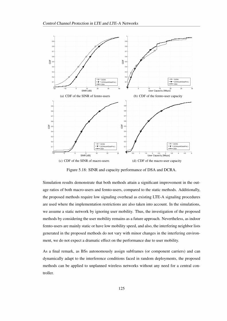
Control Channel Protection in LTE and LTE-A Networks
−20 −10 0 10 20 30 400
0.1
0.2
0.3
0.4
0.5
0.6
0.7
0.8
0.9
1
SINRr[dB]
CD
F
DCRA
DCRA(withDataProt.)
DSA
(a) CDF of the SINR of femto-users
0 5 10 15 20 25 300
0.1
0.2
0.3
0.4
0.5
0.6
0.7
0.8
0.9
1
User(Capacity([Mbps]
CD
F
DCRA
DCRA(withDataProt.)
DSA
(b) CDF of the femto-user capacity
−10 −5 0 5 10 15 200
0.1
0.2
0.3
0.4
0.5
0.6
0.7
0.8
0.9
1
SINRr[dB]
CD
F
DCRA
DCRA(withDataProt.)
DSA
(c) CDF of the SINR of macro-users
0 0.5 1 1.5 2 2.5 3 3.5 4 4.5 50
0.1
0.2
0.3
0.4
0.5
0.6
0.7
0.8
0.9
1
User(Capacity([Mbps]
CD
F
DCRA
DCRA(withDataProt.)
DSA
(d) CDF of the macro-user capacity
Figure 5.18: SINR and capacity performance of DSA and DCRA.
Simulation results demonstrate that both methods attain a significant improvement in the out-
age ratios of both macro-users and femto-users, compared to the static methods. Additionally,
the proposed methods require low signaling overhead as existing LTE-A signaling procedures
are used where the implementation restrictions are also taken into account. In the simulations,
we assume a static network by ignoring user mobility. Thus, the investigation of the proposed
methods by considering the user mobility remains as a future approach. Nevertheless, as indoor
femto-users are mainly static or have low mobility speed, and also, the interfering neighbor lists
generated in the proposed methods do not vary with minor changes in the interfering environ-
ment, we do not expect a dramatic effect on the performance due to user mobility.
As a final remark, as BSs autonomously assign subframes (or component carriers) and can
dynamically adapt to the interference conditions faced in random deployments, the proposed
methods can be applied to unplanned wireless networks without any need for a central con-
troller.
125

Control Channel Protection in LTE and LTE-A Networks
126
Chapter 6Distributed Interference Coordination
6.1 Introduction
Up to now, a detailed overview on femtocell networks and their effects on the overlaid macro-
cell network in terms of capacity and interference are given. In Chapter 4, we discuss the
interference handling approaches introduced with Long-Term Evolution (LTE) and Long-Term
Evolution-Advanced (LTE-A) that can effectively be applied to femtocell networks. LTE sup-
ports inter-cell interference coordination (ICIC) via the use of various signaling and measure-
ments. With the help of the predefined reference signals, the user can measure the received
signal power from base stations (BSs) in its vicinity as well as the signal-to-interference-plus-
noise power ratio (SINR) it experiences and can report these measurements to its serving BS.
Moreover, BSs can exchange information among each other to adapt their resource assign-
ments. With the increased importance of small cells, the coordination between femto-BSs is
maintained in LTE-A by providing a direct X2 interface between femto-BSs and introducing
enhanced inter-cell interference coordination (eICIC) [14]. By taking all restrictions in the stan-
dardization into account, we develop interference mitigation methods for femtocell networks in
Chapter 5. As the correct reception of the control channels in LTE and LTE-A needs the utmost
attention, we mainly give our attention for the protection of the control channels. Unlike Chap-
ter 5, in this chapter and the following one, we give our focus on the improvement of the data
reception. We develop interference mitigation techniques by taking LTE and LTE-A networks
as a reference. However, we do not completely restrict ourselves to the standardizations, hence
relax our assumptions. For instance, we do not take the control channels into account and do
127
Distributed Interference Coordination
not apply any implementation penalty for capacity calculations.
As mentioned in Chapter 4, we consider two approaches for the dynamic interference avoid-
ance; central and distributed approaches. In this chapter, we discuss the distributed interference
mitigation techniques where the resource assignment is done at BSs in parallel instead of gath-
ering all information at one network entity that is responsible for the whole resource assignment
process in the network.
In order to develop a distributed interference management technique with high performance,
users in the network should sense the environment and inform their serving BSs about the
source of interferers. Also, the coordination between BSs should be well established to make
information exchange about their resource assignment policies. It is evident that the more
information is exchanged between the network elements; the better interference is handled.
However, one of the main challenges is the latency of the information exchange between the
network elements. For instance, in LTE and LTE-A, scheduling of resources to users takes
place at every 1 ms, whereas the delay of the X2 signaling between BSs is around 20 ms [67,
92]. Therefore, receiving information from neighboring cells for each scheduling decision is
not possible. Moreover, scanning the spectrum and making measurements at each subframe
increase the complexity at the user side. Last but not least, each information exchange between
users and their serving BSs, and between BSs increases the signaling overhead in a network.
By taking the above-mentioned challenges into account, in this chapter, we discuss various dis-
tributed resource assignment methods and investigate them in terms of the resource efficiency
and signaling overhead by considering the application of those methods to practical networks.
Furthermore, we introduce our proposed method, dynamic and autonomous subband assign-
ment (DASA), where the main motivation is to mitigate high interference between femto-BSs to
protect cell-edge users. Although, we give our interest to femtocell networks and develop our
method based on such networks; the proposed method can be applied to other networks with
minor changes.
We first introduce the system model and the corresponding simulation assumptions in Sec-
tion 6.2. We discuss the related works on the distributed resource assignment in femtocell
networks in Section 6.3. In Section 6.4, a detailed description of the proposed method, DASA,
is given. The simulation results are presented in Section 6.5. Finally, Section 6.6 draws conclu-
sions.
128
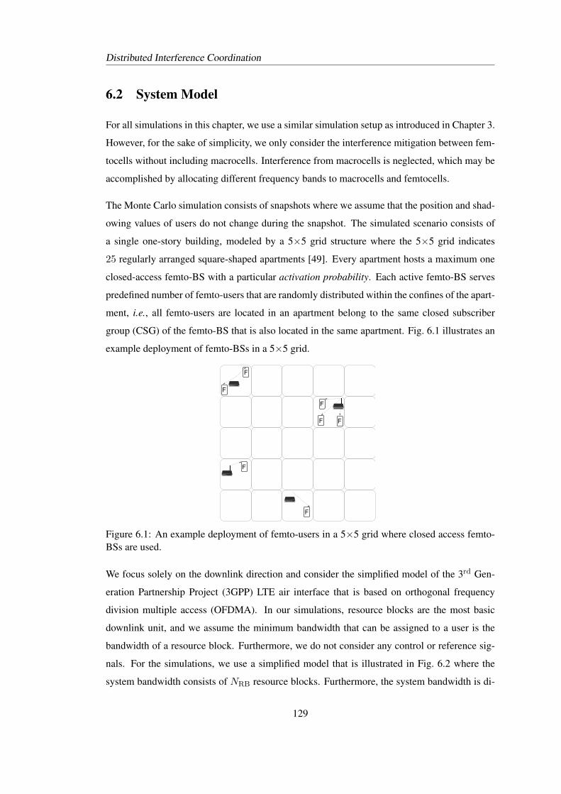
Distributed Interference Coordination
6.2 System Model
For all simulations in this chapter, we use a similar simulation setup as introduced in Chapter 3.
However, for the sake of simplicity, we only consider the interference mitigation between fem-
tocells without including macrocells. Interference from macrocells is neglected, which may be
accomplished by allocating different frequency bands to macrocells and femtocells.
The Monte Carlo simulation consists of snapshots where we assume that the position and shad-
owing values of users do not change during the snapshot. The simulated scenario consists of
a single one-story building, modeled by a 5×5 grid structure where the 5×5 grid indicates
25 regularly arranged square-shaped apartments [49]. Every apartment hosts a maximum one
closed-access femto-BS with a particular activation probability. Each active femto-BS serves
predefined number of femto-users that are randomly distributed within the confines of the apart-
ment, i.e., all femto-users are located in an apartment belong to the same closed subscriber
group (CSG) of the femto-BS that is also located in the same apartment. Fig. 6.1 illustrates an
example deployment of femto-BSs in a 5×5 grid.
F
F
F
F
F
F
F
Figure 6.1: An example deployment of femto-users in a 5×5 grid where closed access femto-BSs are used.
We focus solely on the downlink direction and consider the simplified model of the 3rd Gen-
eration Partnership Project (3GPP) LTE air interface that is based on orthogonal frequency
division multiple access (OFDMA). In our simulations, resource blocks are the most basic
downlink unit, and we assume the minimum bandwidth that can be assigned to a user is the
bandwidth of a resource block. Furthermore, we do not consider any control or reference sig-
nals. For the simulations, we use a simplified model that is illustrated in Fig. 6.2 where the
system bandwidth consists of NRB resource blocks. Furthermore, the system bandwidth is di-
129
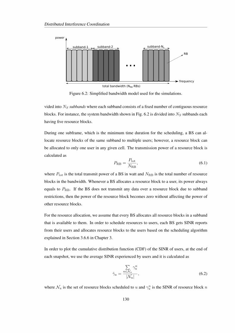
Distributed Interference Coordination
frequency
power
...
total bandwidth (NRB RBs)
RB
subband-1 subband-2 subband-Ns
Figure 6.2: Simplified bandwidth model used for the simulations.
vided into NS subbands where each subband consists of a fixed number of contiguous resource
blocks. For instance, the system bandwidth shown in Fig. 6.2 is divided into NS subbands each
having five resource blocks.
During one subframe, which is the minimum time duration for the scheduling, a BS can al-
locate resource blocks of the same subband to multiple users; however, a resource block can
be allocated to only one user in any given cell. The transmission power of a resource block is
calculated as
PRB =Ptot
NRB, (6.1)
where Ptot is the total transmit power of a BS in watt and NRB is the total number of resource
blocks in the bandwidth. Whenever a BS allocates a resource block to a user, its power always
equals to PRB. If the BS does not transmit any data over a resource block due to subband
restrictions, then the power of the resource block becomes zero without affecting the power of
other resource blocks.
For the resource allocation, we assume that every BS allocates all resource blocks in a subband
that is available to them. In order to schedule resources to users, each BS gets SINR reports
from their users and allocates resource blocks to the users based on the scheduling algorithm
explained in Section 3.6.6 in Chapter 3.
In order to plot the cumulative distribution function (CDF) of the SINR of users, at the end of
each snapshot, we use the average SINR experienced by users and it is calculated as
γu =
∑n∈Nu
γnu
|Nu|, (6.2)
where Nu is the set of resource blocks scheduled to u and γnu is the SINR of resource block n
130
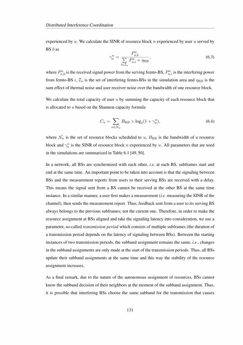
Distributed Interference Coordination
experienced by u. We calculate the SINR of resource block n experienced by user u served by
BS b as
γnu =Pnu,b∑
i∈IuPnu,i + ηRB
, (6.3)
where Pnu,b is the received signal power from the serving femto-BS, Pnu,i is the interfering power
from femto-BS i, Iu is the set of interfering femto-BSs in the simulation area and ηRB is the
sum effect of thermal noise and user receiver noise over the bandwidth of one resource block.
We calculate the total capacity of user u by summing the capacity of each resource block that
is allocated to u based on the Shannon capacity formula
Cu =∑n∈Nu
BRB × log2(1 + γnu ), (6.4)
where Nu is the set of resource blocks scheduled to u, BRB is the bandwidth of a resource
block and γnu is the SINR of resource block n experienced by u. All parameters that are used
in the simulations are summarized in Table 6.1 [49, 50].
In a network, all BSs are synchronized with each other, i.e. at each BS, subframes start and
end at the same time. An important point to be taken into account is that the signaling between
BSs and the measurement reports from users to their serving BSs are received with a delay.
This means the signal sent from a BS cannot be received at the other BS at the same time
instance. In a similar manner, a user first makes a measurement (i.e. measuring the SINR of the
channel), then sends the measurement report. Thus, feedback sent from a user to its serving BS
always belongs to the previous subframes; not the current one. Therefore, in order to make the
resource assignment at BSs aligned and take the signaling latency into consideration, we use a
parameter, so-called transmission period which consists of multiple subframes (the duration of
a transmission period depends on the latency of signaling between BSs). Between the starting
instances of two transmission periods, the subband assignment remains the same, i.e., changes
in the subband assignments are only made at the start of the transmission periods. Thus, all BSs
update their subband assignments at the same time and this way the stability of the resource
assignment increases.
As a final remark, due to the nature of the autonomous assignment of resources, BSs cannot
know the subband decision of their neighbors at the moment of the subband assignment. Thus,
it is possible that interfering BSs choose the same subband for the transmission that causes
131
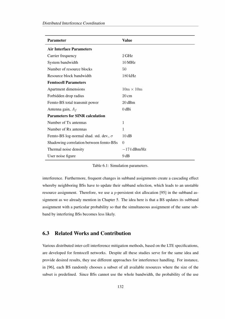
Distributed Interference Coordination
Parameter Value
Air Interface ParametersCarrier frequency 2 GHz
System bandwidth 10 MHz
Number of resource blocks 50
Resource block bandwidth 180 kHz
Femtocell ParametersApartment dimensions 10m× 10m
Forbidden drop radius 20 cm
Femto-BS total transmit power 20 dBm
Antenna gain, Af 0 dBi
Parameters for SINR calculationNumber of Tx antennas 1
Number of Rx antennas 1
Femto-BS log-normal shad. std. dev., σ 10 dB
Shadowing correlation between femto-BSs 0
Thermal noise density −174 dBm/Hz
User noise figure 9 dB
Table 6.1: Simulation parameters.
interference. Furthermore, frequent changes in subband assignments create a cascading effect
whereby neighboring BSs have to update their subband selection, which leads to an unstable
resource assignment. Therefore, we use a p-persistent slot allocation [95] in the subband as-
signment as we already mention in Chapter 5. The idea here is that a BS updates its subband
assignment with a particular probability so that the simultaneous assignment of the same sub-
band by interfering BSs becomes less likely.
6.3 Related Works and Contribution
Various distributed inter-cell interference mitigation methods, based on the LTE specifications,
are developed for femtocell networks. Despite all these studies serve for the same idea and
provide desired results, they use different approaches for interference handling. For instance,
in [96], each BS randomly chooses a subset of all available resources where the size of the
subset is predefined. Since BSs cannot use the whole bandwidth, the probability of the use
132
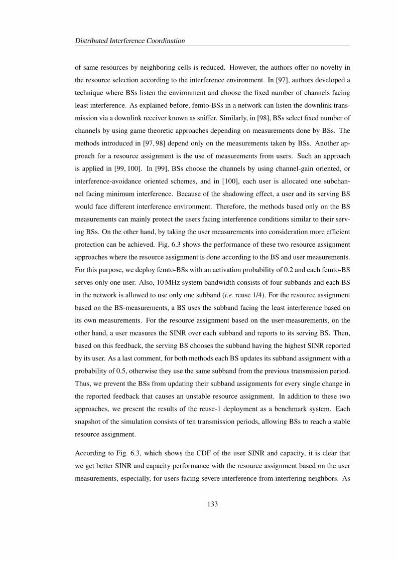
Distributed Interference Coordination
of same resources by neighboring cells is reduced. However, the authors offer no novelty in
the resource selection according to the interference environment. In [97], authors developed a
technique where BSs listen the environment and choose the fixed number of channels facing
least interference. As explained before, femto-BSs in a network can listen the downlink trans-
mission via a downlink receiver known as sniffer. Similarly, in [98], BSs select fixed number of
channels by using game theoretic approaches depending on measurements done by BSs. The
methods introduced in [97, 98] depend only on the measurements taken by BSs. Another ap-
proach for a resource assignment is the use of measurements from users. Such an approach
is applied in [99, 100]. In [99], BSs choose the channels by using channel-gain oriented, or
interference-avoidance oriented schemes, and in [100], each user is allocated one subchan-
nel facing minimum interference. Because of the shadowing effect, a user and its serving BS
would face different interference environment. Therefore, the methods based only on the BS
measurements can mainly protect the users facing interference conditions similar to their serv-
ing BSs. On the other hand, by taking the user measurements into consideration more efficient
protection can be achieved. Fig. 6.3 shows the performance of these two resource assignment
approaches where the resource assignment is done according to the BS and user measurements.
For this purpose, we deploy femto-BSs with an activation probability of 0.2 and each femto-BS
serves only one user. Also, 10 MHz system bandwidth consists of four subbands and each BS
in the network is allowed to use only one subband (i.e. reuse 1/4). For the resource assignment
based on the BS-measurements, a BS uses the subband facing the least interference based on
its own measurements. For the resource assignment based on the user-measurements, on the
other hand, a user measures the SINR over each subband and reports to its serving BS. Then,
based on this feedback, the serving BS chooses the subband having the highest SINR reported
by its user. As a last comment, for both methods each BS updates its subband assignment with a
probability of 0.5, otherwise they use the same subband from the previous transmission period.
Thus, we prevent the BSs from updating their subband assignments for every single change in
the reported feedback that causes an unstable resource assignment. In addition to these two
approaches, we present the results of the reuse-1 deployment as a benchmark system. Each
snapshot of the simulation consists of ten transmission periods, allowing BSs to reach a stable
resource assignment.
According to Fig. 6.3, which shows the CDF of the user SINR and capacity, it is clear that
we get better SINR and capacity performance with the resource assignment based on the user
measurements, especially, for users facing severe interference from interfering neighbors. As
133
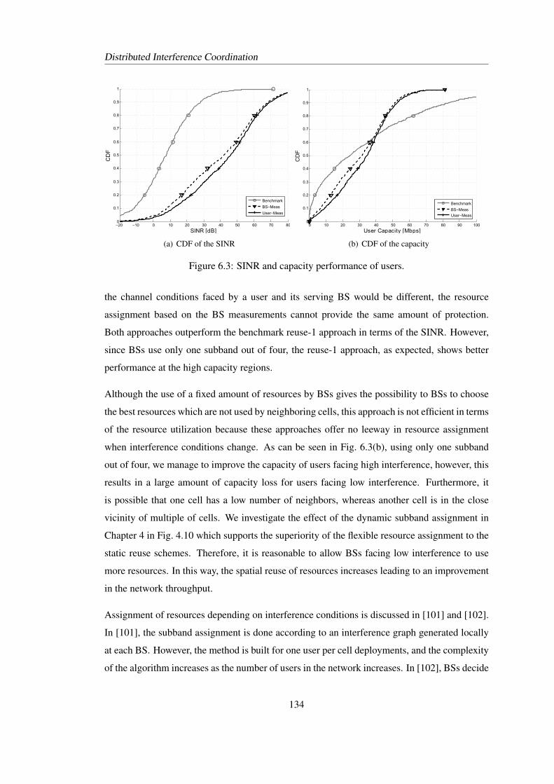
Distributed Interference Coordination
−20 −10 0 10 20 30 40 50 60 70 800
0.1
0.2
0.3
0.4
0.5
0.6
0.7
0.8
0.9
1
SINRM[dB]
CD
F
Benchmark
BS−Meas
User−Meas
(a) CDF of the SINR
0 10 20 30 40 50 60 70 80 90 1000
0.1
0.2
0.3
0.4
0.5
0.6
0.7
0.8
0.9
1
UserhCapacityh[Mbps]
CD
F
Benchmark
BS−Meas
User−Meas
(b) CDF of the capacity
Figure 6.3: SINR and capacity performance of users.
the channel conditions faced by a user and its serving BS would be different, the resource
assignment based on the BS measurements cannot provide the same amount of protection.
Both approaches outperform the benchmark reuse-1 approach in terms of the SINR. However,
since BSs use only one subband out of four, the reuse-1 approach, as expected, shows better
performance at the high capacity regions.
Although the use of a fixed amount of resources by BSs gives the possibility to BSs to choose
the best resources which are not used by neighboring cells, this approach is not efficient in terms
of the resource utilization because these approaches offer no leeway in resource assignment
when interference conditions change. As can be seen in Fig. 6.3(b), using only one subband
out of four, we manage to improve the capacity of users facing high interference, however, this
results in a large amount of capacity loss for users facing low interference. Furthermore, it
is possible that one cell has a low number of neighbors, whereas another cell is in the close
vicinity of multiple of cells. We investigate the effect of the dynamic subband assignment in
Chapter 4 in Fig. 4.10 which supports the superiority of the flexible resource assignment to the
static reuse schemes. Therefore, it is reasonable to allow BSs facing low interference to use
more resources. In this way, the spatial reuse of resources increases leading to an improvement
in the network throughput.
Assignment of resources depending on interference conditions is discussed in [101] and [102].
In [101], the subband assignment is done according to an interference graph generated locally
at each BS. However, the method is built for one user per cell deployments, and the complexity
of the algorithm increases as the number of users in the network increases. In [102], BSs decide
134
Distributed Interference Coordination
on resources they use by using a non-cooperative game theoretic approach, but the actions are
taken by BSs sequentially, so it is difficult to apply this method in practical networks.
In addition to the mentioned techniques, there are also methods developed for LTE-A systems.
One of the primary requirements for LTE-A is to support a transmission bandwidth of up to
100 MHz. This is achieved via the carrier aggregation where multiple blocks of LTE bandwidth,
named as component carriers, are amalgamated to obtain a wider usable spectrum [20,21]. Nat-
urally, with the additional degree of freedom that arises through the carrier aggregation, inter-
ference mitigation by optimizing the selection of the subset of all available component carriers
among the contending BSs is expected to develop into an attractive research topic. A compo-
nent carrier selection method depending on the interference environment of BSs in an LTE-A
system is introduced in [103–106]. The methods in [103–105] result in an excessive signaling
between BSs. In [106], the required signaling overhead is reduced with promising results, but
the proposed method does not offer any explicit protection of cell-edge users in densely de-
ployed uncoordinated networks. Another component carrier assignment method is developed
in [107] where each BS calculates its resource assignment sequentially, and the method has
high complexity in terms of required signaling. Furthermore, in [108], a BS assigns a new
component carrier as long as the capacity gain in their cells is greater than the sum capacity
loss in neighboring cells. This prevents the greedy use of resources by BSs and introduces fair
use of resources among BSs since a BS cannot use an extra resource if the resource causes high
interference to other cells. On the other hand, the proposed scheme assumes that the carrier
allocation is done iteratively and during each iteration a BS tries only one carrier.
Our main objective is to develop a method that each BS in a network adapts its resource usage
on-the-fly, so as to improve the capacity of cell-edge users without causing a sharp decrease
in the overall network capacity. Also, we seek for a method with low signaling overhead and
compatible with LTE and LTE-A networks. Based on these requirements, in this chapter, a
novel DASA is investigated. The proposed DASA is a distributed and dynamic resource as-
signment method that is particularly well suited for randomly deployed, decentralized femto-
cell networks. The main purpose is to protect mobile users located near the cell boundary from
detrimental downlink interference originating from neighboring BSs without compromising the
system spectral efficiency. The proposed method is designed such that the interference protec-
tion does not coincide with an intolerable reduction in the attainable spatial reuse of radio re-
sources. System-level simulations reveal that with DASA cell-edge capacities are significantly
135
Distributed Interference Coordination
boosted without a sharp decrease in average system throughput.
6.4 Dynamic and Autonomous Subband Assignment
From our previous discussions, we know that we can improve the SINR of users by restricting
a BS from using all subbands. However, we also show that the more resources we restrict
at BSs, the lower capacity performance we get. Hence, it is important to keep the balance
between the level of interference and the resource utilization. For instance, assume a network
where all BSs use only one subband. Assume that BS b is using subband 1 and starts to use
subband 2 in addition to subband 1. This would eventually enhance the capacity in the given
cell due to an increase in the amount of resources used for the transmission. However, using an
extra subband at BS b causes additional interference to cells which are already using subband
2. Depending on the network environment, the use of subband 2 may cause high interference
to BS b’s neighbors, so the capacity improvement in BS b becomes less reasonable when the
overall network capacity is considered. On the other hand, it would also be possible that the
neighbors of BS b do not face severe interference from BS b. Thus, using an extra subband
at BS b becomes beneficial in terms of the capacity as the trade-off is on a bearable level.
Therefore, in our proposed method, namely DASA, the main idea is allowing a BS to use
additional resources as long as the overall capacity in the network does not decrease. Hence, we
can protect cell-edge users by considering the overall system capacity. Furthermore, in DASA,
the subband assignment is done on an event triggered basis. Thus, subbands are updated only
if there is a change in the interference environment.
Assume that BS b serves user u and u can provide SINR measurements to b for each subband.
Based on feedback from u, BS b can calculate the achievable spectral efficiency of u over
subband s as
Rsu = log2(1 + γsu), (6.5)
where γsu is the SINR of subband s that user u measured and reported to b. Given Rsu, if any
resource block from subband s is scheduled to u, the data rate at user u amounts to
Cu = BRBRsu, (6.6)
where BRB is the bandwidth of a resource block. Since there is a direct relation between the
data rate and the spectral efficiency, increasing the total spectral efficiencies of users, without
136
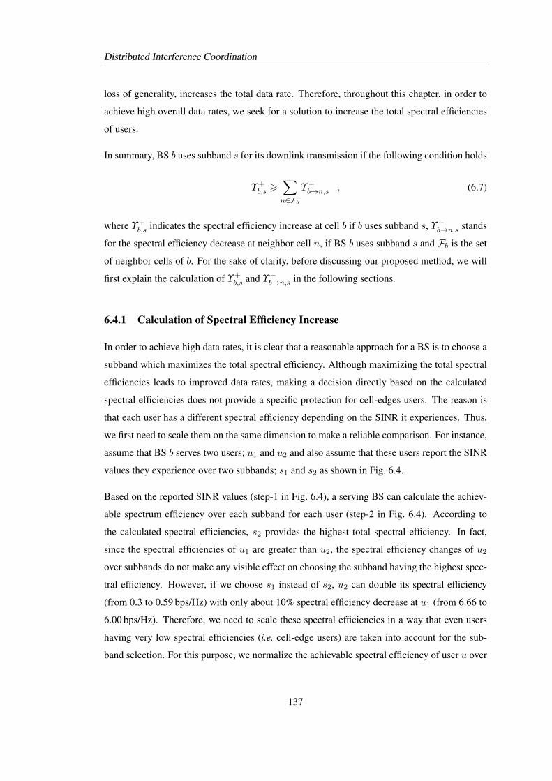
Distributed Interference Coordination
loss of generality, increases the total data rate. Therefore, throughout this chapter, in order to
achieve high overall data rates, we seek for a solution to increase the total spectral efficiencies
of users.
In summary, BS b uses subband s for its downlink transmission if the following condition holds
Υ+b,s >
∑n∈Fb
Υ−b→n,s , (6.7)
where Υ+b,s indicates the spectral efficiency increase at cell b if b uses subband s, Υ−b→n,s stands
for the spectral efficiency decrease at neighbor cell n, if BS b uses subband s and Fb is the set
of neighbor cells of b. For the sake of clarity, before discussing our proposed method, we will
first explain the calculation of Υ+b,s and Υ−b→n,s in the following sections.
6.4.1 Calculation of Spectral Efficiency Increase
In order to achieve high data rates, it is clear that a reasonable approach for a BS is to choose a
subband which maximizes the total spectral efficiency. Although maximizing the total spectral
efficiencies leads to improved data rates, making a decision directly based on the calculated
spectral efficiencies does not provide a specific protection for cell-edges users. The reason is
that each user has a different spectral efficiency depending on the SINR it experiences. Thus,
we first need to scale them on the same dimension to make a reliable comparison. For instance,
assume that BS b serves two users; u1 and u2 and also assume that these users report the SINR
values they experience over two subbands; s1 and s2 as shown in Fig. 6.4.
Based on the reported SINR values (step-1 in Fig. 6.4), a serving BS can calculate the achiev-
able spectrum efficiency over each subband for each user (step-2 in Fig. 6.4). According to
the calculated spectral efficiencies, s2 provides the highest total spectral efficiency. In fact,
since the spectral efficiencies of u1 are greater than u2, the spectral efficiency changes of u2
over subbands do not make any visible effect on choosing the subband having the highest spec-
tral efficiency. However, if we choose s1 instead of s2, u2 can double its spectral efficiency
(from 0.3 to 0.59 bps/Hz) with only about 10% spectral efficiency decrease at u1 (from 6.66 to
6.00 bps/Hz). Therefore, we need to scale these spectral efficiencies in a way that even users
having very low spectral efficiencies (i.e. cell-edge users) are taken into account for the sub-
band selection. For this purpose, we normalize the achievable spectral efficiency of user u over
137
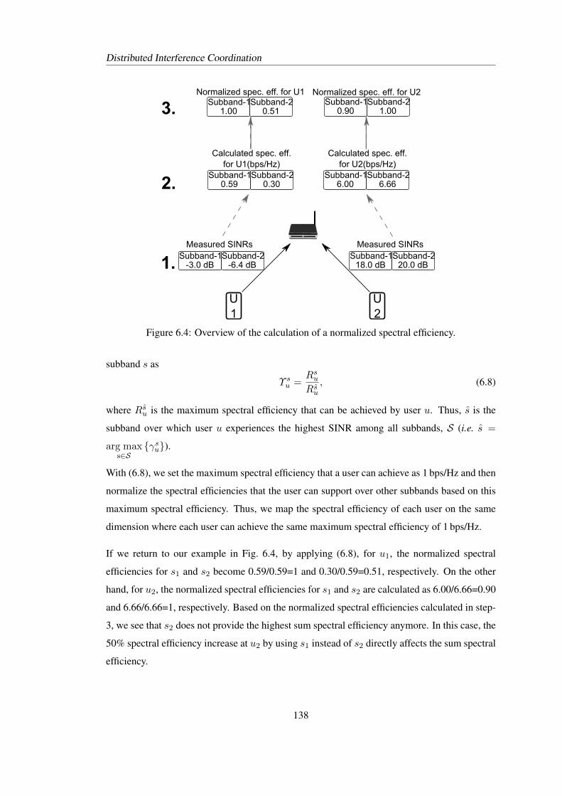
Distributed Interference Coordination
U1
-3.0pdBSubband-1
MeasuredpSINRs
-6.4pdBSubband-2
U2
18.0pdBSubband-1
MeasuredpSINRs
20.0pdBSubband-2
0.59pSubband-1
Calculatedpspec.peff.forpU1mbps/Hzi
0.30Subband-2
6.00pSubband-1
Calculatedpspec.peff.forpU2mbps/Hzi
6.66Subband-2
Normalizedpspec.peff.pforpU1
1.00pSubband-1
0.51Subband-2
Normalizedpspec.peff.pforpU2p
0.90pSubband-1
1.00Subband-2
1.
2.
3.
Figure 6.4: Overview of the calculation of a normalized spectral efficiency.
subband s as
Υ su =RsuRsu
, (6.8)
where Rsu is the maximum spectral efficiency that can be achieved by user u. Thus, s is the
subband over which user u experiences the highest SINR among all subbands, S (i.e. s =
arg maxs∈S
{γsu}).
With (6.8), we set the maximum spectral efficiency that a user can achieve as 1 bps/Hz and then
normalize the spectral efficiencies that the user can support over other subbands based on this
maximum spectral efficiency. Thus, we map the spectral efficiency of each user on the same
dimension where each user can achieve the same maximum spectral efficiency of 1 bps/Hz.
If we return to our example in Fig. 6.4, by applying (6.8), for u1, the normalized spectral
efficiencies for s1 and s2 become 0.59/0.59=1 and 0.30/0.59=0.51, respectively. On the other
hand, for u2, the normalized spectral efficiencies for s1 and s2 are calculated as 6.00/6.66=0.90
and 6.66/6.66=1, respectively. Based on the normalized spectral efficiencies calculated in step-
3, we see that s2 does not provide the highest sum spectral efficiency anymore. In this case, the
50% spectral efficiency increase at u2 by using s1 instead of s2 directly affects the sum spectral
efficiency.
138
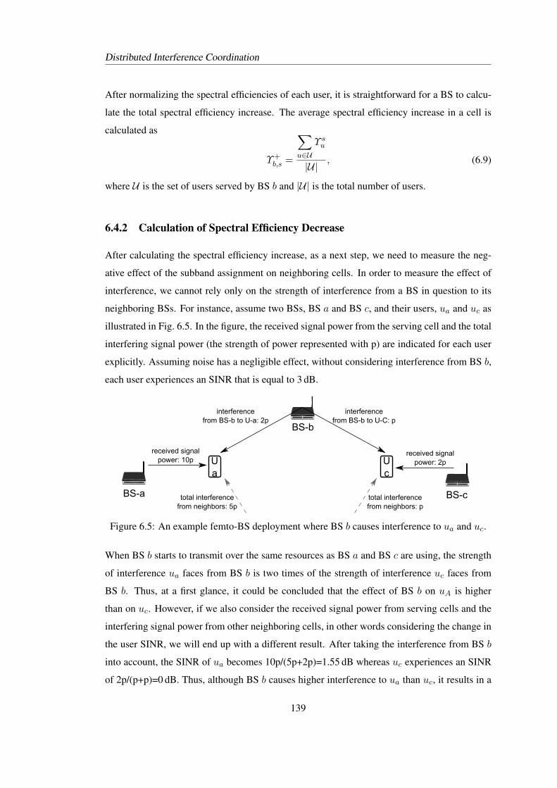
Distributed Interference Coordination
After normalizing the spectral efficiencies of each user, it is straightforward for a BS to calcu-
late the total spectral efficiency increase. The average spectral efficiency increase in a cell is
calculated as
Υ+b,s =
∑u∈U
Υ su
|U|, (6.9)
where U is the set of users served by BS b and |U| is the total number of users.
6.4.2 Calculation of Spectral Efficiency Decrease
After calculating the spectral efficiency increase, as a next step, we need to measure the neg-
ative effect of the subband assignment on neighboring cells. In order to measure the effect of
interference, we cannot rely only on the strength of interference from a BS in question to its
neighboring BSs. For instance, assume two BSs, BS a and BS c, and their users, ua and uc as
illustrated in Fig. 6.5. In the figure, the received signal power from the serving cell and the total
interfering signal power (the strength of power represented with p) are indicated for each user
explicitly. Assuming noise has a negligible effect, without considering interference from BS b,
each user experiences an SINR that is equal to 3 dB.
Ua
Uc
total interference from neighbors: 5p
BS-a
received signal power: 10p
interference from BS-b to U-a: 2p
received signal power: 2p
total interference from neighbors: p
BS-c
BS-b
interference from BS-b to U-C: p
Figure 6.5: An example femto-BS deployment where BS b causes interference to ua and uc.
When BS b starts to transmit over the same resources as BS a and BS c are using, the strength
of interference ua faces from BS b is two times of the strength of interference uc faces from
BS b. Thus, at a first glance, it could be concluded that the effect of BS b on uA is higher
than on uc. However, if we also consider the received signal power from serving cells and the
interfering signal power from other neighboring cells, in other words considering the change in
the user SINR, we will end up with a different result. After taking the interference from BS b
into account, the SINR of ua becomes 10p/(5p+2p)=1.55 dB whereas uc experiences an SINR
of 2p/(p+p)=0 dB. Thus, although BS b causes higher interference to ua than uc, it results in a
139
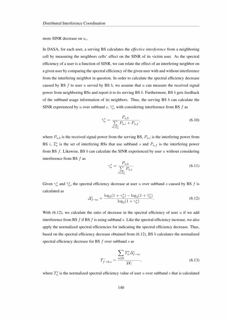
Distributed Interference Coordination
more SINR decrease on uc.
In DASA, for each user, a serving BS calculates the effective interference from a neighboring
cell by measuring the neighbors cells’ effect on the SINR of its victim user. As the spectral
efficiency of a user is a function of SINR, we can relate the effect of an interfering neighbor on
a given user by comparing the spectral efficiency of the given user with and without interference
from the interfering neighbor in question. In order to calculate the spectral efficiency decrease
caused by BS f to user u served by BS b, we assume that u can measure the received signal
power from neighboring BSs and report it to its serving BS b. Furthermore, BS b gets feedback
of the subband usage information of its neighbors. Thus, the serving BS b can calculate the
SINR experienced by u over subband s, γsu, with considering interference from BS f as
γsu =Pu,b∑
i∈IsuPu,i + Pu,f
, (6.10)
where Pu,b is the received signal power from the serving BS, Pu,i is the interfering power from
BS i, Isu is the set of interfering BSs that use subband s and Pu,f is the interfering power
from BS f . Likewise, BS b can calculate the SINR experienced by user u without considering
interference from BS f as
γsu =Pu,b∑
i∈IsuPu,i
. (6.11)
Given γsu and γsu, the spectral efficiency decrease at user u over subband s caused by BS f is
calculated as
∆sf→u =
log2(1 + γsu)− log2(1 + γsu)
log2(1 + γsu). (6.12)
With (6.12), we calculate the ratio of decrease in the spectral efficiency of user u if we add
interference from BS f if BS f is using subband s. Like the spectral efficiency increase, we also
apply the normalized spectral efficiencies for indicating the spectral efficiency decrease. Thus,
based on the spectral efficiency decrease obtained from (6.12), BS b calculates the normalized
spectral efficiency decrease for BS f over subband s as
Υ−f→b,s =
∑u∈U
Υ su∆sf→u
|U|, (6.13)
where Υ su is the normalized spectral efficiency value of user u over subband s that is calculated
140
Distributed Interference Coordination
by using (6.8).
Each BS calculates the spectral efficiency decrease for each subband for each interfering neigh-
bor cell and signals to its neighbors. As a last remark, if BS b is not using subband s, then it
does not calculate any spectral efficiency decrease as the use of s by neighboring cells does not
make any effect on its data rate.
6.4.3 Application of DASA
DASA is applied at each BS in two steps; the first step is the subband assignment, and the
second step is the calculation of the spectral efficiency decreases. These two steps, subband
assignment and spectral efficiency decrease calculations, are applied by BSs over a period of
two transmission periods. For the first transmission period, the subband assignment is done,
whereas, for the second transmission period, BSs calculate the spectral efficiency decrease
depending on the updated subband assignment. Fig. 6.6 illustrates the application of DASA by
a BS and the required feedback at two consecutive transmission periods.
step-1:subband
assignment
transmission period t
No change on the assigned subbands
step-2:data rate decrease
calculationdata rate
decrease informationfrom neighbors
SINR form users
SINR & received interferenceform users
subband assignmentinformation
from neighbors
subband assignmentinformation
to neighbors
transmission period t+1
step-1:subband
assignment
SINR form users
data ratedecrease information
from neighbors
data ratedecrease information
to neighbors
Figure 6.6: Overview of the application of DASA by a BS and the required feedback at trans-mission periods.
As can be seen in the figure, the subband assignment done by a BS remains the same during two
consecutive transmission periods. For instance, if the subband assignment is done just before
transmission period t, then the BS calculates the corresponding spectral efficiency decrease be-
fore transmission period t+1 without changing its subband assignment. The reason of applying
these two steps separately is due to the effect of the signaling delay between BSs. Instead of
separating these two steps over two transmission periods, assume that BSs calculate the spectral
efficiency decrease and the subband assignment together before each transmission period. In
such a case, before transmission period t, each BS in the network calculates the spectral effi-
141
Distributed Interference Coordination
ciency decreases of its own users depending on the measurements (SINR reports and subband
usage information of neighboring BSs) from transmission period t − 1. Then, each BS sends
the corresponding spectral efficiency decrease information to its neighboring cells during trans-
mission period t. Consequently, for the subband assignment before transmission period t + 1,
BSs receive spectral efficiency decrease values based on the measurements from transmission
period t−1. However, it is possible that BSs may change their subband assignments in-between
or users may experience different channel conditions. This eventually affects the reliability of
the subband assignment at BSs as they receive outdated feedback. For this reason, we separate
these two steps and after BSs update their subband assignments for the transmission period t,
they inform their neighbors about their subband assignments, i.e. which subbands they are us-
ing. Then, during transmission period t, all users make the SINR measurements according to
the updated subband assignment and report to their serving BSs with the received interfering
signal power measurements from neighboring BSs. Thus, at the end of transmission period t,
each BS has the SINR and subband usage information based on the current subband assign-
ment. Additionally, BSs can accurately calculate the spectral efficiency decrease and send the
corresponding reports to their neighbors during transmission period t + 1. Since BSs do not
change their subband assignment during transmission period t + 1, BSs update their subband
assignment before transmission period t+ 2 with up to date feedback.
6.4.3.1 Step-1: Assignment of Subbands
In order to assign subbands in DASA, a BS needs SINR reports from its served users over each
subband. Furthermore, in addition to the SINR reports, the information of Υ−b→n,s coming from
neighboring cells is also required. The BS in question first calculates the spectral efficiency
increase for each subband. Then, according to the spectral efficiency decrease information from
neighboring cells, it uses subbands which hold the condition in (6.7) for the next transmission
period. Thus, we give a flexibility to the BS to use the available subbands as long as it does not
cause high interference to its neighbors. If no subband provides the condition in (6.7), the BS
uses the subband providing the minimum∑n∈Nb
Υ−b→n,s − Υ+b,s value.
In DASA, BSs update their subband assignments with a probability. Thus, each BS updates
its subband assignment if the probability condition holds; otherwise it continues to use the
subband assignment from the previous transmission period. In this way, we prevent a BS from
reacting to each single change in the received feedback proactively and changing its subband
142
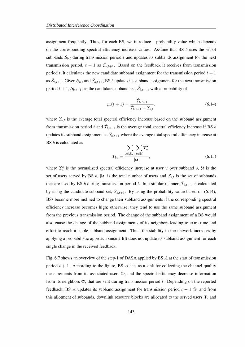
Distributed Interference Coordination
assignment frequently. Thus, for each BS, we introduce a probability value which depends
on the corresponding spectral efficiency increase values. Assume that BS b uses the set of
subbands Sb,t during transmission period t and updates its subbands assignment for the next
transmission period, t + 1 as Sb,t+1. Based on the feedback it receives from transmission
period t, it calculates the new candidate subband assignment for the transmission period t + 1
as Sb,t+1. Given Sb,t and Sb,t+1, BS b updates its subband assignment for the next transmission
period t+ 1, Sb,t+1, as the candidate subband set, Sb,t+1, with a probability of
pb(t+ 1) =Υb,t+1
Υb,t+1 + Υb,t, (6.14)
where Υb,t is the average total spectral efficiency increase based on the subband assignment
from transmission period t and Υb,t+1 is the average total spectral efficiency increase if BS b
updates its subband assignment as Sb,t+1 where the average total spectral efficiency increase at
BS b is calculated as
Υb,t =
∑s∈Sb,t
∑u∈U
Υ su
|U|, (6.15)
where Υ su is the normalized spectral efficiency increase at user u over subband s, U is the
set of users served by BS b, |U| is the total number of users and Sb,t is the set of subbands
that are used by BS b during transmission period t. In a similar manner, Υb,t+1 is calculated
by using the candidate subband set, Sb,t+1. By using the probability value based on (6.14),
BSs become more inclined to change their subband assignments if the corresponding spectral
efficiency increase becomes high; otherwise, they tend to use the same subband assignment
from the previous transmission period. The change of the subband assignment of a BS would
also cause the change of the subband assignments of its neighbors leading to extra time and
effort to reach a stable subband assignment. Thus, the stability in the network increases by
applying a probabilistic approach since a BS does not update its subband assignment for each
single change in the received feedback.
Fig. 6.7 shows an overview of the step-1 of DASA applied by BS A at the start of transmission
period t + 1. According to the figure, BS A acts as a sink for collecting the channel quality
measurements from its associated users ¬, and the spectral efficiency decrease information
from its neighbors , that are sent during transmission period t. Depending on the reported
feedback, BS A updates its subband assignment for transmission period t + 1 ®, and from
this allotment of subbands, downlink resource blocks are allocated to the served users ¯, and
143
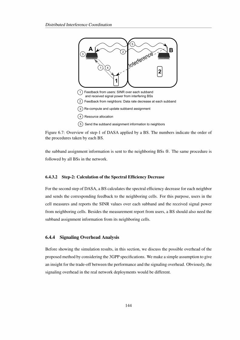
Distributed Interference Coordination
1
A B
21
2
4
5
Interference3
1 Feedbackpfrompusers:pSINRpoverpeachpsubbandppandpreceivedpsignalppowerpfrompinterferingpBSsp
2 Feedbackpfrompneighbors:pDatapratepdecreasepatpeachpsubband
3 Re-computepandpupdatepsubbandpassignment
4 Resourcepallocation
5 Sendpthepsubbandpassignmentpinformationptopneighbors
Figure 6.7: Overview of step-1 of DASA applied by a BS. The numbers indicate the order ofthe procedures taken by each BS.
the subband assignment information is sent to the neighboring BSs °. The same procedure is
followed by all BSs in the network.
6.4.3.2 Step-2: Calculation of the Spectral Efficiency Decrease
For the second step of DASA, a BS calculates the spectral efficiency decrease for each neighbor
and sends the corresponding feedback to the neighboring cells. For this purpose, users in the
cell measures and reports the SINR values over each subband and the received signal power
from neighboring cells. Besides the measurement report from users, a BS should also need the
subband assignment information from its neighboring cells.
6.4.4 Signaling Overhead Analysis
Before showing the simulation results, in this section, we discuss the possible overhead of the
proposed method by considering the 3GPP specifications. We make a simple assumption to give
an insight for the trade-off between the performance and the signaling overhead. Obviously, the
signaling overhead in the real network deployments would be different.
144
Distributed Interference Coordination
6.4.4.1 Duration of Transmission Periods
As illustrated in Fig. 6.6, in DASA, a BS expects feedback from its users and neighbors at each
transmission period. Please note that the transmission period is different from the subframe
which stands for the scheduling period in the time domain. The duration of a transmission
period can vary from one subframe to multiple subframes depending on the network require-
ments and the latency in the signaling. For instance, in LTE and LTE-A, BSs exchange load
information between each other via an X2 interface having 20 ms latency [67, 92]. Also, in
order to report the received signal power and SINR, a user needs some time interval to make
the measurements.
The signaling overhead of DASA mainly depends on the duration of the transmission period.
Assume that we set the duration of a transmission period as 1 ms (i.e. one subframe) where
each user in the network should report the received signal power level from interfering BSs and
SINR of each subband at each subframe. In this way, a BS can track the every change in the
environment (such as the change of the location of users) before each scheduling decision. On
the other hand, sending feedback at each subframe, apparently, leads to a high signaling over-
head. By increasing the duration of the transmission period, for example, from 1 ms to 20 ms,
we roughly reduce the signaling overhead by 20 times. Since users in a femtocell network are
mostly located indoors, they do not change their locations quickly. Thus, updating the subband
assignment at each 20 ms would not cause a visible degradation at the performance of DASA.
6.4.4.2 Received Signal Power Levels
Each user in a network is expected to report the received signal power level from BSs in its
vicinity. In order to evaluate the overhead, we refer to the reference signal received power
(RSRP) message defined in 3GPP. As mentioned in Chapter 4, the RSRP indicates the signal
strength of a BS measured by a user where the RSRP values are quantized into 98 levels [89].
Thus, the corresponding overhead per report is assumed as 7 bits. Since the user should report
the received power from each neighboring cell, the total overhead equals to 7×Nb bits where
Nb is the total number of the neighboring BSs. Since each report stands for the received power
from one BS, the number of reports sent by a user depends on the interfering environment. In
densely deployed networks, a user senses more BSs, thus sends more reports.
In LTE and LTE-A networks, users are required to report the received signal power from BSs
145
Distributed Interference Coordination
in their vicinities via the RSRP for handover purposes. Thus, in such a case, we do not require
any extra signaling for DASA. The only restriction here is that, in real deployments, a user can
report a limited number of BSs at a given time.
6.4.4.3 SINR per Subband
In DASA, we also require SINR levels measured by users for calculation of the spectral effi-
ciency increase. If the SINR report of one subband requires NSINR bits then for each user the
total overhead becomes NSINR×NS where NS is the total number of subbands to be reported.
As mentioned in Chapter 4, in LTE and LTE-A networks, users send the channel-quality indi-
cator (CQI) reports for improving the scheduling at their serving BSs. These reports indicate
the SINR levels in term of modulation and coding schemes. Therefore, in a given network,
if users report CQI values for each subband at each transmission period, then DASA does not
cause any extra signaling overhead.
6.4.4.4 Spectral Efficiency Decrease Information
Each BS sends feedback of the corresponding spectral efficiency decrease to its neighbors at
every second transmission period. This value varies between 0 and 1 as the normalized spectral
efficiencies are used in DASA. The total overhead then equals to Ndec ×NS ×Nb where Ndec
is the number of bits required to indicate the spectral efficiency decrease, NS is the number
of subbands and Nb is the number of neighboring BSs. The value of Ndec depends on the
quantization levels used for describing the spectral efficiencies. It is clear that increasing Ndec
improves the accuracy of the feedback but also increases the signaling overhead.
6.4.4.5 Subband Usage Information
After updating the subband assignment, each BS informs its neighbors about its subband usage
during every second transmission period. Such information can be sent via a bitmap where each
bit indicates a subband like the relative narrowband transmit power (RNTP) indicators defined
in LTE and LTE-A. Thus, for NS subbands, the overhead of the subband information signaling
becomesNS×Nb whereNS is the total number of subbands andNb is the number of neighbors
to be informed.
146
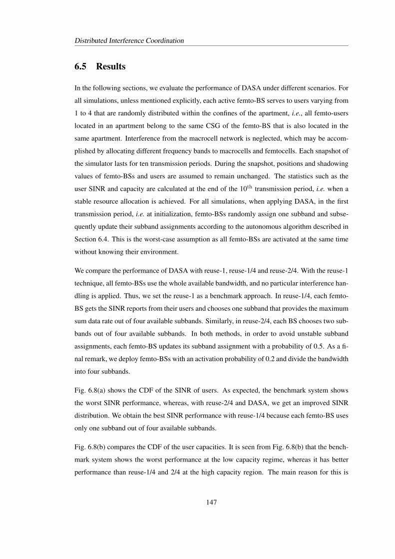
Distributed Interference Coordination
6.5 Results
In the following sections, we evaluate the performance of DASA under different scenarios. For
all simulations, unless mentioned explicitly, each active femto-BS serves to users varying from
1 to 4 that are randomly distributed within the confines of the apartment, i.e., all femto-users
located in an apartment belong to the same CSG of the femto-BS that is also located in the
same apartment. Interference from the macrocell network is neglected, which may be accom-
plished by allocating different frequency bands to macrocells and femtocells. Each snapshot of
the simulator lasts for ten transmission periods. During the snapshot, positions and shadowing
values of femto-BSs and users are assumed to remain unchanged. The statistics such as the
user SINR and capacity are calculated at the end of the 10th transmission period, i.e. when a
stable resource allocation is achieved. For all simulations, when applying DASA, in the first
transmission period, i.e. at initialization, femto-BSs randomly assign one subband and subse-
quently update their subband assignments according to the autonomous algorithm described in
Section 6.4. This is the worst-case assumption as all femto-BSs are activated at the same time
without knowing their environment.
We compare the performance of DASA with reuse-1, reuse-1/4 and reuse-2/4. With the reuse-1
technique, all femto-BSs use the whole available bandwidth, and no particular interference han-
dling is applied. Thus, we set the reuse-1 as a benchmark approach. In reuse-1/4, each femto-
BS gets the SINR reports from their users and chooses one subband that provides the maximum
sum data rate out of four available subbands. Similarly, in reuse-2/4, each BS chooses two sub-
bands out of four available subbands. In both methods, in order to avoid unstable subband
assignments, each femto-BS updates its subband assignment with a probability of 0.5. As a fi-
nal remark, we deploy femto-BSs with an activation probability of 0.2 and divide the bandwidth
into four subbands.
Fig. 6.8(a) shows the CDF of the SINR of users. As expected, the benchmark system shows
the worst SINR performance, whereas, with reuse-2/4 and DASA, we get an improved SINR
distribution. We obtain the best SINR performance with reuse-1/4 because each femto-BS uses
only one subband out of four available subbands.
Fig. 6.8(b) compares the CDF of the user capacities. It is seen from Fig. 6.8(b) that the bench-
mark system shows the worst performance at the low capacity regime, whereas it has better
performance than reuse-1/4 and 2/4 at the high capacity region. The main reason for this is
147
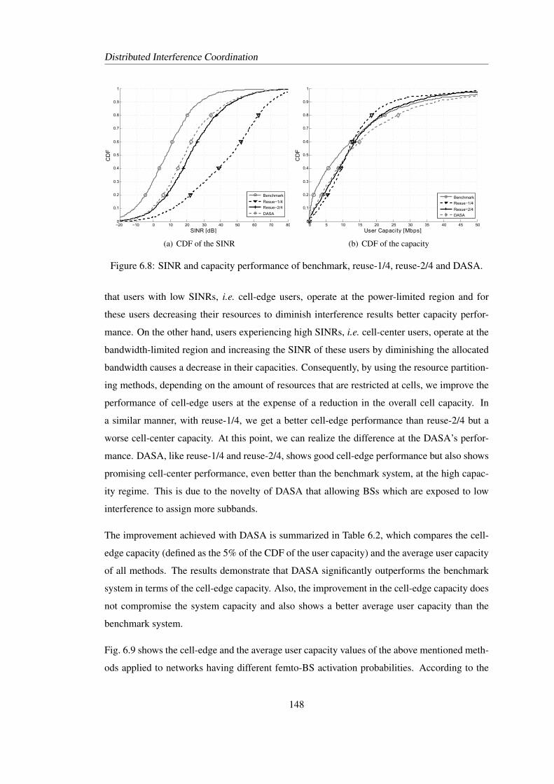
Distributed Interference Coordination
−20 −10 0 10 20 30 40 50 60 70 800
0.1
0.2
0.3
0.4
0.5
0.6
0.7
0.8
0.9
1
SINRs[dB]
CD
F
Benchmark
Resue−1/4
Resue−2/4
DASA
(a) CDF of the SINR
0 5 10 15 20 25 30 35 40 45 500
0.1
0.2
0.3
0.4
0.5
0.6
0.7
0.8
0.9
1
UserhCapacityh[Mbps]
CD
F
Benchmark
Resue−1/4
Resue−2/4
DASA
(b) CDF of the capacity
Figure 6.8: SINR and capacity performance of benchmark, reuse-1/4, reuse-2/4 and DASA.
that users with low SINRs, i.e. cell-edge users, operate at the power-limited region and for
these users decreasing their resources to diminish interference results better capacity perfor-
mance. On the other hand, users experiencing high SINRs, i.e. cell-center users, operate at the
bandwidth-limited region and increasing the SINR of these users by diminishing the allocated
bandwidth causes a decrease in their capacities. Consequently, by using the resource partition-
ing methods, depending on the amount of resources that are restricted at cells, we improve the
performance of cell-edge users at the expense of a reduction in the overall cell capacity. In
a similar manner, with reuse-1/4, we get a better cell-edge performance than reuse-2/4 but a
worse cell-center capacity. At this point, we can realize the difference at the DASA’s perfor-
mance. DASA, like reuse-1/4 and reuse-2/4, shows good cell-edge performance but also shows
promising cell-center performance, even better than the benchmark system, at the high capac-
ity regime. This is due to the novelty of DASA that allowing BSs which are exposed to low
interference to assign more subbands.
The improvement achieved with DASA is summarized in Table 6.2, which compares the cell-
edge capacity (defined as the 5% of the CDF of the user capacity) and the average user capacity
of all methods. The results demonstrate that DASA significantly outperforms the benchmark
system in terms of the cell-edge capacity. Also, the improvement in the cell-edge capacity does
not compromise the system capacity and also shows a better average user capacity than the
benchmark system.
Fig. 6.9 shows the cell-edge and the average user capacity values of the above mentioned meth-
ods applied to networks having different femto-BS activation probabilities. According to the
148
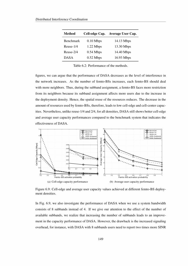
Distributed Interference Coordination
Method Cell-edge Cap. Average User Cap.
Benchmark 0.10 Mbps 14.13 Mbps
Reuse-1/4 1.22 Mbps 13.30 Mbps
Reuse-2/4 0.54 Mbps 14.40 Mbps
DASA 0.52 Mbps 16.93 Mbps
Table 6.2: Performance of the methods.
figures, we can argue that the performance of DASA decreases as the level of interference in
the network increases. As the number of femto-BSs increases, each femto-BS should deal
with more neighbors. Thus, during the subband assignment, a femto-BS faces more restriction
from its neighbors because its subband assignment affects more users due to the increase in
the deployment density. Hence, the spatial reuse of the resources reduces. The decrease in the
amount of resources used by femto-BSs, therefore, leads to low cell-edge and cell-center capac-
ities. Nevertheless, unlike reuse-1/4 and 2/4, for all densities, DASA still shows better cell-edge
and average user capacity performances compared to the benchmark system that indicates the
effectiveness of DASA.
0.2 0.3 0.4 0.5 0.6 0.7 0.8 0.9 10
0.2
0.4
0.6
0.8
1
1.2
1.4
Femto−BSdactivationdprobability
Cel
ldEd
gedC
apac
ityd[M
bps]
BenchmarkReuse−1/4Reuse−2/4DASA−4subbandsDASA−8subbands
0.6 0.7 0.8 0.9 10
0.01
0.02
0.03
0.04
0.05
0.06
(a) Cell-edge capacity performance
0.2 0.3 0.4 0.5 0.6 0.7 0.8 0.9 12
4
6
8
10
12
14
16
18
Femto−BSUactivationUprobability
Ave
rag
eUU
serU
Cap
acit
yU[M
bp
s]
BenchmarkReuse−1/4Reuse−2/4DASA−4subbandsDASA−8subbands
(b) Average user capacity performance
Figure 6.9: Cell-edge and average user capacity values achieved at different femto-BS deploy-ment densities.
In Fig. 6.9, we also investigate the performance of DASA when we use a system bandwidth
consists of 8 subbands instead of 4. If we give our attention to the effect of the number of
available subbands, we realize that increasing the number of subbands leads to an improve-
ment in the capacity performance of DASA. However, the drawback is the increased signaling
overhead, for instance, with DASA with 8 subbands users need to report two times more SINR
149
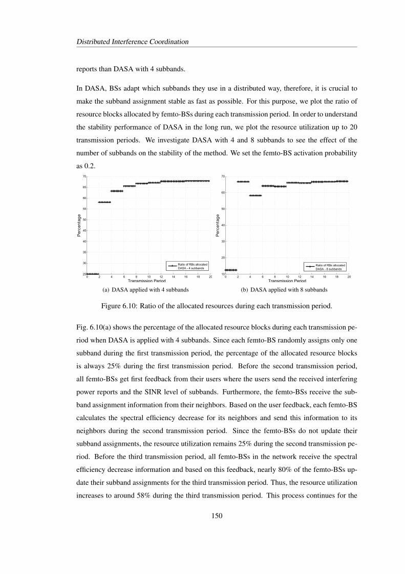
Distributed Interference Coordination
reports than DASA with 4 subbands.
In DASA, BSs adapt which subbands they use in a distributed way, therefore, it is crucial to
make the subband assignment stable as fast as possible. For this purpose, we plot the ratio of
resource blocks allocated by femto-BSs during each transmission period. In order to understand
the stability performance of DASA in the long run, we plot the resource utilization up to 20
transmission periods. We investigate DASA with 4 and 8 subbands to see the effect of the
number of subbands on the stability of the method. We set the femto-BS activation probability
as 0.2.
0 2 4 6 8 10 12 14 16 18 2025
30
35
40
45
50
55
60
65
70
Transmission-Period
Per
cen
tag
e
Ratio-of-RBs-allocatedDASA---4-subbands
(a) DASA applied with 4 subbands
0 2 4 6 8 10 12 14 16 18 2010
20
30
40
50
60
70
Transmission-Period
Per
cen
tag
e
Ratio-of-RBs-allocatedDASA---8-subbands
(b) DASA applied with 8 subbands
Figure 6.10: Ratio of the allocated resources during each transmission period.
Fig. 6.10(a) shows the percentage of the allocated resource blocks during each transmission pe-
riod when DASA is applied with 4 subbands. Since each femto-BS randomly assigns only one
subband during the first transmission period, the percentage of the allocated resource blocks
is always 25% during the first transmission period. Before the second transmission period,
all femto-BSs get first feedback from their users where the users send the received interfering
power reports and the SINR level of subbands. Furthermore, the femto-BSs receive the sub-
band assignment information from their neighbors. Based on the user feedback, each femto-BS
calculates the spectral efficiency decrease for its neighbors and send this information to its
neighbors during the second transmission period. Since the femto-BSs do not update their
subband assignments, the resource utilization remains 25% during the second transmission pe-
riod. Before the third transmission period, all femto-BSs in the network receive the spectral
efficiency decrease information and based on this feedback, nearly 80% of the femto-BSs up-
date their subband assignments for the third transmission period. Thus, the resource utilization
increases to around 58% during the third transmission period. This process continues for the
150
Distributed Interference Coordination
subsequent transmission periods and the amount of changes in the subband assignment between
the transmission periods become negligible after transmission period 10. Furthermore, if we
consider the percentage of subbands of which femto-BSs update the usage before each trans-
mission period (i.e. during transmission period t + 1, a femto-BS begins to use a subband that
is not active during transmission period t or the other way around), we observe that the femto-
BSs update the usage of around 5% of all subbands before starting transmission period 11 and
this percentage drops to less than 1% before transmission period 19. Besides, only 1.5% of
the femto-BSs in the network change their subband assignments before transmission period 19.
Thus, we can conclude that as femto-BSs learn their environment and get feedback from their
users and neighbors, the system reaches to a stable point in terms of subband assignment.
We observe the same pattern with DASA with 8 subbands as shown in Fig. 6.10(b). As the
femto-BSs use only one subband out of eight at the beginning of the simulation, the resource
utilization becomes 12.5% during the first two transmission periods. Additionally, since the
number of subbands is increased to eight, there are more choices for the femto-BSs for the
subband assignment. Thus, the ratio of the femto-BSs that update their subband assignments
is higher than the percentage obtained with DASA with 4 subbands. For instance, before the
third transmission period, 85% of all femto-BSs update their subband assignments, and this
ratio decreases as the femto-BSs learn their neighbors’ decisions. Before transmission period
19, only 2.5% of the femto-BSs update their subband assignments; however, this ratio is 1.5%
for DASA with 4 subbands. Thus, we can conclude that increasing the number of subbands
also increases the time required to reach a stable subband assignment.
It is important to mention that we are considering a scenario where all femto-BSs are turned
on at the same time without knowing any information about their environment. However, if we
consider a femto-BS that enters an active network where other femto-BSs already know their
environments, then it is expected that the resource assignment reaches a stable point in a shorter
time. Furthermore, the traffic conditions also affect the stability of DASA. In our simulations,
femto-BSs compete for all subbands. If they adapt their subband usages depending on their
traffic loads, the amount of interference in a network decreases. Thus, more efficient resource
assignment is achieved.
151
Distributed Interference Coordination
6.6 Conclusion
In this chapter, we develop an interference mitigation technique that can be applied by BSs
in a distributed way without any need of a central controller. We aim at decreasing interfer-
ence between cells by wise partitioning of resources among them. However, there are several
challenges such as quick convergence to the stable resource assignment, low signaling over-
head and high resource utilization. Besides, the technique should be applicable to unplanned
wireless networks that are characterized by varying interference conditions.
In proposed DASA, we give flexibility to BSs so that they can dynamically adapt to the inter-
ference conditions faced in random deployments. Simulation results demonstrate that DASA
attains a significant improvement for cell-edge users as well as system capacities. Furthermore,
the system reaches a stable point in a short time.
The signaling we assume in our system model are mainly based on the existing LTE and LTE-A
signaling procedures that are already used by BSs for other purposes. For instance, in LTE
and LTE-A, in order to improve the scheduling performance, BSs receive the information of
subband SINR measurements from each user via the CQI reports [71]. Similarly, for handover
processes, a BS should know whether its user receives a stronger signal from neighboring BSs.
For this purpose, users measure the received signal power from near BSs and report their serving
BSs with the RSRPs [88]. Only the signaling between BSs are not implicitly specified in the
standards, but they can be used with minor changes on the signals (such as the RNTP [71]
indicator) that are already defined for ICIC and eICIC techniques. Furthermore, the proposed
DASA method is applied by BSs, and it does not bring any functional complexity on the user
side where users only report the channel conditions and the interfering neighbors that is aligned
with the specifications. Therefore, DASA can be applied to LTE and LTE-A networks with
minor effects on the BS side.
It is worth to mention that the use of DASA is not limited to the frequency-domain as shown in
this chapter, but can be used with any other domains such as the time or code-domains. Last but
not least, we consider LTE femtocell networks as a basis to explain DASA; however, the pro-
posed method can be expanded to any other uncoordinated networks or macrocell deployments
with small changes.
152
Chapter 7Centralized Interference Coordination
7.1 Introduction
In Chapter 6, distributed interference avoidance techniques are discussed, and the novel dy-
namic and autonomous subband assignment (DASA) is introduced. In this chapter, we turn our
attention to central approaches where resources are assigned to base stations (BSs) (or to users)
by means of a central controller.
In a given network, the central controller gets the feedback from all BSs (or all users) thereby
having global knowledge of the network. Thus, it can assign resources in a more efficient way
which is the main advantage of the central approach. Besides, unlike the distributed approach,
only one network entity is responsible for assigning the resources; thus, the network reaches a
stable resource assignment in a short time.
The main drawback of the central approach is the increased complexity at the central controller
that is critical for real networks where the central controller should reach a solution in terms of
milliseconds. Therefore, the practical methods aim to achieve a resource assignment as close
as possible to the optimum solution with low complexity such as by assigning a limited amount
of resources to cells according to the traffic demands [109]. One of the well-known approaches
followed for this purpose is the use of graph coloring algorithms which are computationally
efficient means for interference aware resource assignment. Graph coloring algorithms color
the nodes of a graph with a minimum number of colors such that no two connected nodes have
the same color. If the relation between network entities is mapped onto a graph, graph coloring
153
Centralized Interference Coordination
facilitates resource assignment by assuming each color as a different resource where two nodes
connected in the graph must not use the same resource.
In this chapter, we address the interference avoidance by a novel centrally controlled resource
partitioning methods. The developed methods are based on a low-complex graph coloring
algorithm that assigns resources with high resource utilization. Similar to DASA proposed in
Chapter 6, the primary objective is to protect users that are located near the cell boundary of two
or more femtocells from detrimental downlink interference, especially for randomly deployed
wireless networks. We provide system-level simulations for comparison, and results reveal
that with the proposed methods, cell-edge capacities are significantly boosted without causing
unacceptable degradation in average system throughput. As a system model, we use femtocells
but the proposed methods can be applied to other uncoordinated networks with minor changes.
In this chapter, we give a comprehensive overview of the graph coloring algorithms in Sec-
tion 7.2. We also investigate different approaches of applying the graph coloring approach for
resource assignment in this section. We introduce our methods in Sections 7.3 and Sections 7.4
where we use two distinct techniques serving for separate performance requirements. In Sec-
tion 7.3, we aim at low complexity and signaling overhead whereas, in Section 7.4, we seek for
the high resource utilization; hence, high system capacity. In addition to the central method, in
Section 7.5, we introduce another method that is the hybrid of central and distributed methods.
Lastly, we finalize the chapter with Section 7.6
7.2 Graph Coloring as an Interference Mitigation Technique
7.2.1 Graph Coloring
Graph theory is generally used in mathematics and science to model the relation between ob-
jects. A graph consists of nodes (or vertices) where the nodes are connected to each other with
edges. Coloring the graph elements such as the nodes with constraints is known as graph col-
oring or vertex coloring. The idea of graph coloring is using the minimum number of colors in
a way that no two connected nodes have the same color.
In a given graph, the nodes connected to each other with an edge are called adjacent nodes (in
this context we also use the term neighboring nodes), and the degree of a node v indicates the
number of adjacent nodes connected to v. Thus, an isolated node has a degree of zero [110].
154
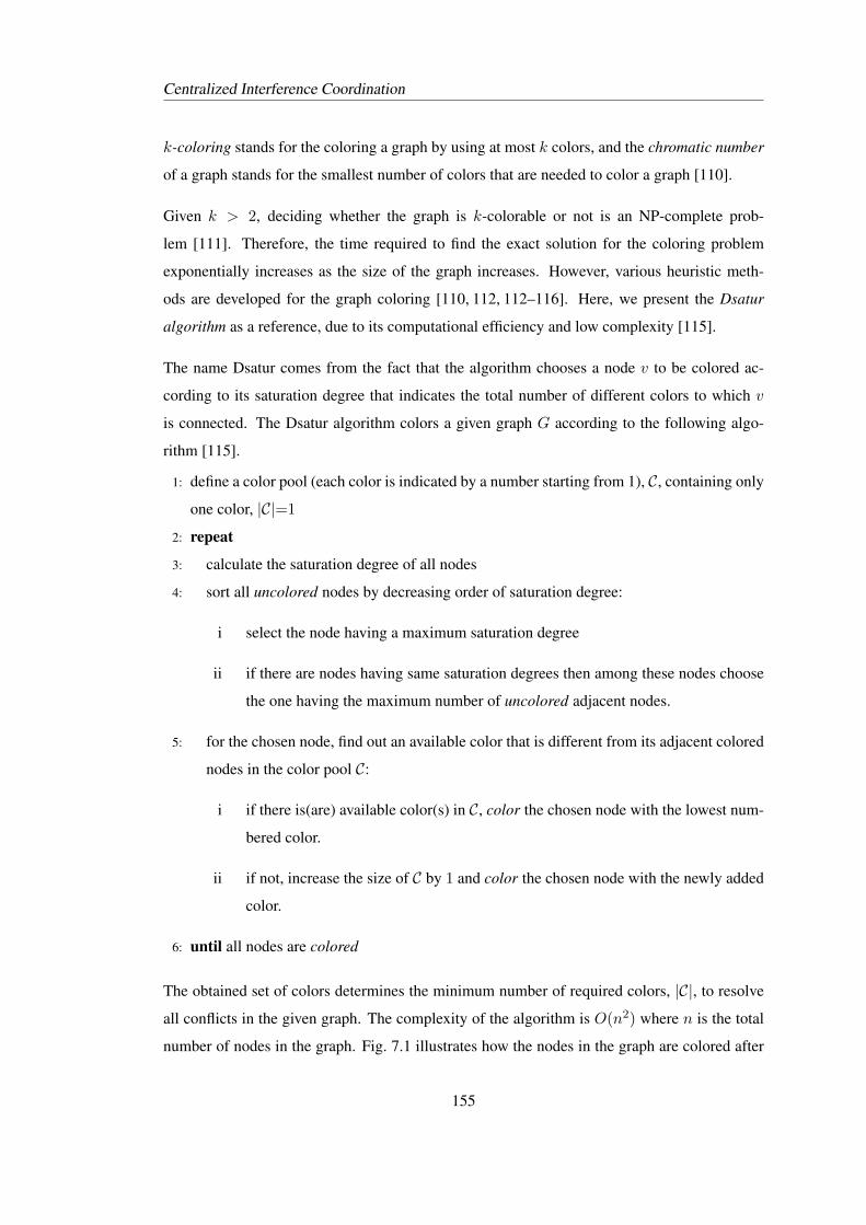
Centralized Interference Coordination
k-coloring stands for the coloring a graph by using at most k colors, and the chromatic number
of a graph stands for the smallest number of colors that are needed to color a graph [110].
Given k > 2, deciding whether the graph is k-colorable or not is an NP-complete prob-
lem [111]. Therefore, the time required to find the exact solution for the coloring problem
exponentially increases as the size of the graph increases. However, various heuristic meth-
ods are developed for the graph coloring [110, 112, 112–116]. Here, we present the Dsatur
algorithm as a reference, due to its computational efficiency and low complexity [115].
The name Dsatur comes from the fact that the algorithm chooses a node v to be colored ac-
cording to its saturation degree that indicates the total number of different colors to which v
is connected. The Dsatur algorithm colors a given graph G according to the following algo-
rithm [115].
1: define a color pool (each color is indicated by a number starting from 1), C, containing only
one color, |C|=1
2: repeat
3: calculate the saturation degree of all nodes
4: sort all uncolored nodes by decreasing order of saturation degree:
i select the node having a maximum saturation degree
ii if there are nodes having same saturation degrees then among these nodes choose
the one having the maximum number of uncolored adjacent nodes.
5: for the chosen node, find out an available color that is different from its adjacent colored
nodes in the color pool C:
i if there is(are) available color(s) in C, color the chosen node with the lowest num-
bered color.
ii if not, increase the size of C by 1 and color the chosen node with the newly added
color.
6: until all nodes are colored
The obtained set of colors determines the minimum number of required colors, |C|, to resolve
all conflicts in the given graph. The complexity of the algorithm is O(n2) where n is the total
number of nodes in the graph. Fig. 7.1 illustrates how the nodes in the graph are colored after
155
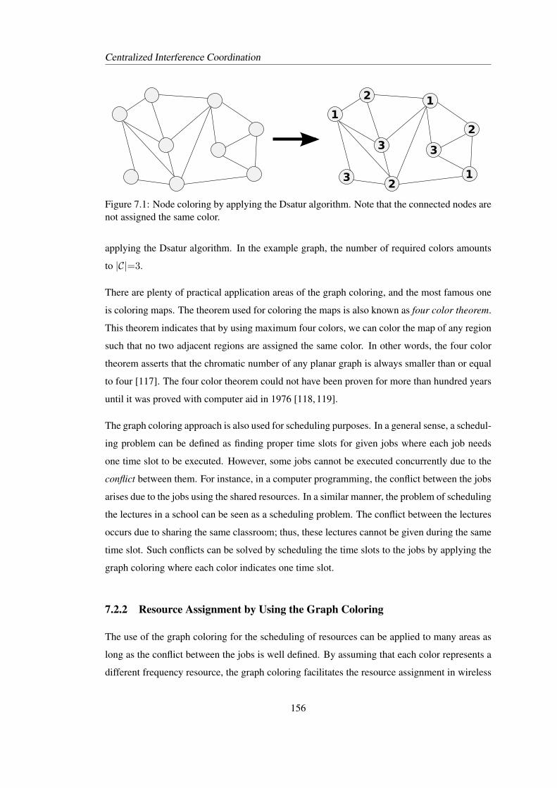
Centralized Interference Coordination
11
1
2
2
2
3
3 3
Figure 7.1: Node coloring by applying the Dsatur algorithm. Note that the connected nodes arenot assigned the same color.
applying the Dsatur algorithm. In the example graph, the number of required colors amounts
to |C|=3.
There are plenty of practical application areas of the graph coloring, and the most famous one
is coloring maps. The theorem used for coloring the maps is also known as four color theorem.
This theorem indicates that by using maximum four colors, we can color the map of any region
such that no two adjacent regions are assigned the same color. In other words, the four color
theorem asserts that the chromatic number of any planar graph is always smaller than or equal
to four [117]. The four color theorem could not have been proven for more than hundred years
until it was proved with computer aid in 1976 [118, 119].
The graph coloring approach is also used for scheduling purposes. In a general sense, a schedul-
ing problem can be defined as finding proper time slots for given jobs where each job needs
one time slot to be executed. However, some jobs cannot be executed concurrently due to the
conflict between them. For instance, in a computer programming, the conflict between the jobs
arises due to the jobs using the shared resources. In a similar manner, the problem of scheduling
the lectures in a school can be seen as a scheduling problem. The conflict between the lectures
occurs due to sharing the same classroom; thus, these lectures cannot be given during the same
time slot. Such conflicts can be solved by scheduling the time slots to the jobs by applying the
graph coloring where each color indicates one time slot.
7.2.2 Resource Assignment by Using the Graph Coloring
The use of the graph coloring for the scheduling of resources can be applied to many areas as
long as the conflict between the jobs is well defined. By assuming that each color represents a
different frequency resource, the graph coloring facilitates the resource assignment in wireless
156
Centralized Interference Coordination
networks. The graph contains a node for every user or a BS and an edge for the conflict between
the nodes indicating that same resources should not be assigned to these nodes because of high
interference. In this context, the generated graph is also called interference graph.
In a given network, in order to generate an interference graph, it is essential to define the nodes
and the conflicting conditions between the nodes precisely. Depending on the definition of
the nodes and edges, different interference graphs can be built for the same network. Fig. 7.2
illustrates an example network where three different approaches are followed to map the inter-
ference relation onto three different interference graphs.
The performance of the applied algorithm is highly based on the generated interference graph,
and the number of the available colors (resources) to assign the nodes. Thus, in the following
sections, we explain the effect of them on the performance of the graph coloring algorithm.
7.2.2.1 Defining Nodes
Nodes in an interference graph can either represent users or BSs. We name the interference
graph constructed with users as user-based interference graph. Interference graphs I [120] and
III [121] in Fig. 7.2 are examples of such kind of graphs. In a similar manner, if the nodes
in the interference graph represent BSs, then it is called BS-based interference graph. The
interference graph II [122] in Fig. 7.2 is generated according to BSs. If the graph is constructed
by users, resource allocation to the users is directly made by the central controller. On the other
hand, if BSs are used at the interference graph, the central controller assigns the resources to
the BSs and then the BSs allocate the available resources to their users.
Assigning resources directly to users leads to more efficient resource utilization as the controller
has global information of each user in the network. Nevertheless, making the resource assign-
ment according to the user-based interference graph increases the complexity at the controller
and the network. One reason is that, with the user-based interference graph, the controller
should deal with a larger graph with more nodes. Such large graphs, ultimately, increase the
time complexity of the applied graph-coloring algorithm and introduce substantial delays. Sec-
ondly, the central controller needs feedback from all users in the network; thus, the signaling
overhead increases. Last but not least, the user-based interference graph needs to be updated
whenever the users in the network change their location. Therefore, with the user-based inter-
ference graph, the resource assignment needs to be frequently updated that results in further
157
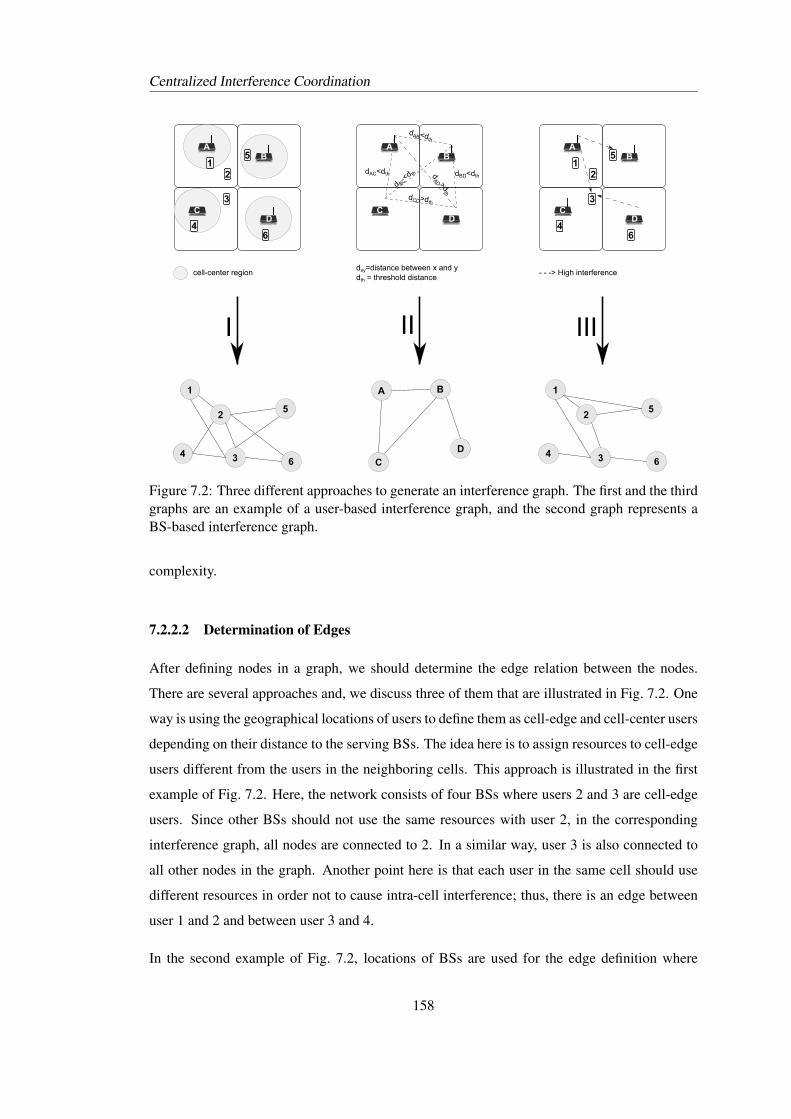
Centralized Interference Coordination
1
2
34
5
6
A B
C
D
1
2
34
5
6
I II III
AB
CD
dAB<dth
dAC<dth
d BC<d th
dCD>dth
dBD<dth dAD >d
th
dxy=distance between x and ydth = threshold distance
12
3
6
5
4
AB
CD
cell-center region
12
3
6
5
4
AB
CD
- - -> High interference
Figure 7.2: Three different approaches to generate an interference graph. The first and the thirdgraphs are an example of a user-based interference graph, and the second graph represents aBS-based interference graph.
complexity.
7.2.2.2 Determination of Edges
After defining nodes in a graph, we should determine the edge relation between the nodes.
There are several approaches and, we discuss three of them that are illustrated in Fig. 7.2. One
way is using the geographical locations of users to define them as cell-edge and cell-center users
depending on their distance to the serving BSs. The idea here is to assign resources to cell-edge
users different from the users in the neighboring cells. This approach is illustrated in the first
example of Fig. 7.2. Here, the network consists of four BSs where users 2 and 3 are cell-edge
users. Since other BSs should not use the same resources with user 2, in the corresponding
interference graph, all nodes are connected to 2. In a similar way, user 3 is also connected to
all other nodes in the graph. Another point here is that each user in the same cell should use
different resources in order not to cause intra-cell interference; thus, there is an edge between
user 1 and 2 and between user 3 and 4.
In the second example of Fig. 7.2, locations of BSs are used for the edge definition where
158
Centralized Interference Coordination
the BSs located with a distance smaller than a predefined threshold distance are connected
in the interference graph. According to the example, the distances between BSs A, B and C
and between B and D are smaller than the predefined threshold distance. Therefore, in the
corresponding interference graph, nodes A, B and C are connected since they should not be
assigned the same resources. Similarly, nodes B and D are also connected in the graph.
The last example defines the edges between the nodes based on the interference level caused
from one node to another if the same resource is assigned to these nodes. In this case, there is a
predefined interference threshold and if assigning a resource to one user causes interference to
another user above the threshold level, these users are assigned different resources. In the given
example, BS A causes high interference to users 3 and 5; thus, it should use different resources
than what is assigned to users 3 and 5. Similarly, BS D causes high interference to user 3 and
BS D should not use the same resources that are assigned to user 3. As a final remark, users at
the same cell are also connected because they are restricted to use different resources in order
to remove the intra-cell interference.
The approaches presented in Fig. 7.2 indicate that depending on the definition of nodes and
the conflict between them, distinct interference graphs are obtained from the same network
deployment. Therefore, each approach results in a different resource assignment hence different
system performance. Generating the interference graphs according to the user measurements
instead of relying on the distance or the BS measurements gives more reliable results. Because
of the shadowing effect, users in the same cell would face distinct interference conditions than
their serving BSs. Therefore, the interference graph generated through the third approach in
Fig. 7.2 gives more realistic interference relation than the first and second approaches.
It is also possible to generate an interference graph with weighted edges. In such an approach,
all nodes are connected with each other where each edge has a weight. The weight of an edge
can be calculated according to the distance between nodes or the interference level received
from neighboring nodes. Using weighted edges leads to an increase in the resource utilization
since the controller has more information on the interference environment of BSs and users.
In order to calculate the weights for each edge, the central controller requires additional feed-
back such as channel conditions, level of interference. Also, whenever the channel conditions
change, the weights of edges at the controller should be updated.
159
Centralized Interference Coordination
7.2.2.3 Number of Available Colors
The total number of resources (such as subbands and resource blocks) is typically a predefined
network planning parameter. Therefore, a graph coloring algorithm works in a desired way as
long as the number of available resources is larger or equal to the number of colors required
to color the graph, i.e. the total number of resources to be assigned to nodes should be at least
equal to the chromatic number of the graph (smallest number of colors that are needed to color
a graph).
As a final remark, in the ‘conventional’ graph coloring methods, each node is allocated only one
partition of the available resources. For instance, givenN available frequency bands, each node
is assigned 1/N of the available resources, regardless of the number of neighboring nodes they
are connected to. Such an assignment of the resources causes inefficient resource utilization es-
pecially for situations where N is large. In order to improve the resource utilization, flexibility
in the number of the allocated resources per node is, therefore, desirable. It is clear that in order
to increase the spatial reuse of resources, a node that does not suffer from severe interference
should be able to use more resources without causing high interference to its neighbors.
7.2.3 Related Graph Coloring Works
The use of the interference graph for interference mitigation has been investigated by various
works. In [120], authors developed a resource assignment method for macrocell networks by
combining the fractional frequency reuse technique with the graph coloring algorithm. In this
method, users that are located out of the predefined cell-center radius are defined as a cell-
edge user and they are assigned different resources than the users in the neighboring cells
(connected in the interference graph). However, the graph coloring algorithm assigns only one
partition of the available resources to each user without considering any resource utilization.
In [121, 123, 124], the interference graph is constructed according to the interference relation
between users, but the assignment of resources to the users differs in each method. In [123], the
resource assignment is done randomly, whereas, in [121], a graph coloring algorithm is applied
to the interference graph and in [124], the method is further improved where optimization in
the resource assignment is introduced. However, all the mentioned methods [120,121,123,124]
assume a hexagonal deployment where the number and location of BSs are static. Thus, they
are mainly applicable to macrocell networks.
160
Centralized Interference Coordination
In [125, 126], resources are allocated to users based on the interference graph with weighted
edges where the weights are calculated according to the path loss between users and the inter-
fering BSs. Nevertheless, the proposed method fits hexagonal macrocell deployments where
the number and position of the interfering BSs are static.
Graph coloring methods that are particularly developed for femtocell networks are discussed
in [122, 127, 128]. In these methods, an interference graph used for the resource assignment is
generated by using the location of BSs. As discussed previously, such resource assignment is
not effective because users can face different interference conditions than their serving BS.
By taking the advantages and drawbacks of the graph coloring algorithms mentioned up to now,
in this chapter, we propose a graph-based dynamic frequency reuse (GB-DFR) algorithm that
is suited to small cell scenarios with the objective of increasing the cell-edge capacity whilst
maintaining high resource utilization. In the proposed GB-DFR, each BS in the network is
connected to the central controller and sends the identity of its interfering BSs to the controller.
The central controller maps this information onto the interference graph. As mentioned in
the previous section, the conventional graph coloring algorithms do not consider the resource
utilization. Therefore, we apply a modified graph coloring algorithm that takes the usage ef-
ficiency of resources into account and strikes a balance between interference protection and
spatial frequency reuse of resources. For this purpose, we introduce flexibility in the number of
assigned resources that depends on the interference conditions of each base station. Those BSs
facing low interference are assigned more resources; thus, high resource utilization is achieved.
GB-DFR can be applied by using a BS-based interference graph or user-based interference
graph depending on the network conditions and requirements. In the first method, in the gen-
erated interference graph, each node represents a BS and the controller assigns the available
resources to BSs. We call this method GB-DFR with the BS-based interference graph. In the
second method, the central controller assigns resources directly to users by generating a user-
based interference graph where each user is represented by a node in the graph. We call this
method GB-DFR with the user-based interference graph. We aim to decrease the complexity
at the central controller and the overall signaling overhead in the network with the first method,
whereas in the second method, we pursuit high throughput performances especially for multi-
user deployments.
In addition to GB-DFR, we also introduce a second algorithm namely extended graph-based
161
Centralized Interference Coordination
dynamic frequency reuse (eGB-DFR) that is the hybrid of central and distributed interference
handling approaches and makes use of the powerful parts of each approach.
7.3 GB-DFR with the BS-Based Interference Graph
In this type of GB-DFR, after BSs inform the identities of the interfering neighbors to the
central controller, the central controller generates an interference graph where nodes stand for
BSs. The controller assigns subbands to BSs, and it feeds the assigned subbands information
back to each BS. In the end, each BS is informed of its own subband information, and it
allocates the resource blocks of its assigned subbands to its users.
7.3.1 System Model
We use the same system model as we explain in Chapter 6. The simulated area modeled by
a 5×5 grid structure [49] where each apartment can have only one closed-access femto-BS.
As in Chapter 6, we consider only femtocell networks and interference from the macrocell
network is neglected. We use the Long-Term Evolution (LTE) air interface where the available
frequency bandwidth consists of multiple subbands and each subband comprises a fixed number
of resource blocks as illustrated in 6.2. A detailed explanation of the calculation of signal-to-
interference-plus-noise power ratio (SINR) and user capacity and the corresponding simulation
parameters can be found in Section 6.2 of Chapter 6.
We assume that users in the network can differentiate between the received signals from various
BSs in their vicinity with the help of BS-specific reference signals and can report them to the
serving BS. Also, for the resource allocation, BSs rely on the SINR measurements from their
own users. For this purpose, each user in the network, periodically reports the SINR levels it
experiences over each subband to its serving BS.
Each BS in a network is connected to a central controller. For instance, as explained in
Chapter 3, in LTE and Long-Term Evolution-Advanced (LTE-A) networks, a HeNB-gateway
(HeNB-GW) [30] can be used as a central controller. In order to apply the central resource
assignment, we use a two-way signaling between BSs and the central controller. Each BS
sends the information of its interfering neighbors to the central controller and the central con-
troller sends the corresponding subband assignment information to the BSs. Thus, different
162
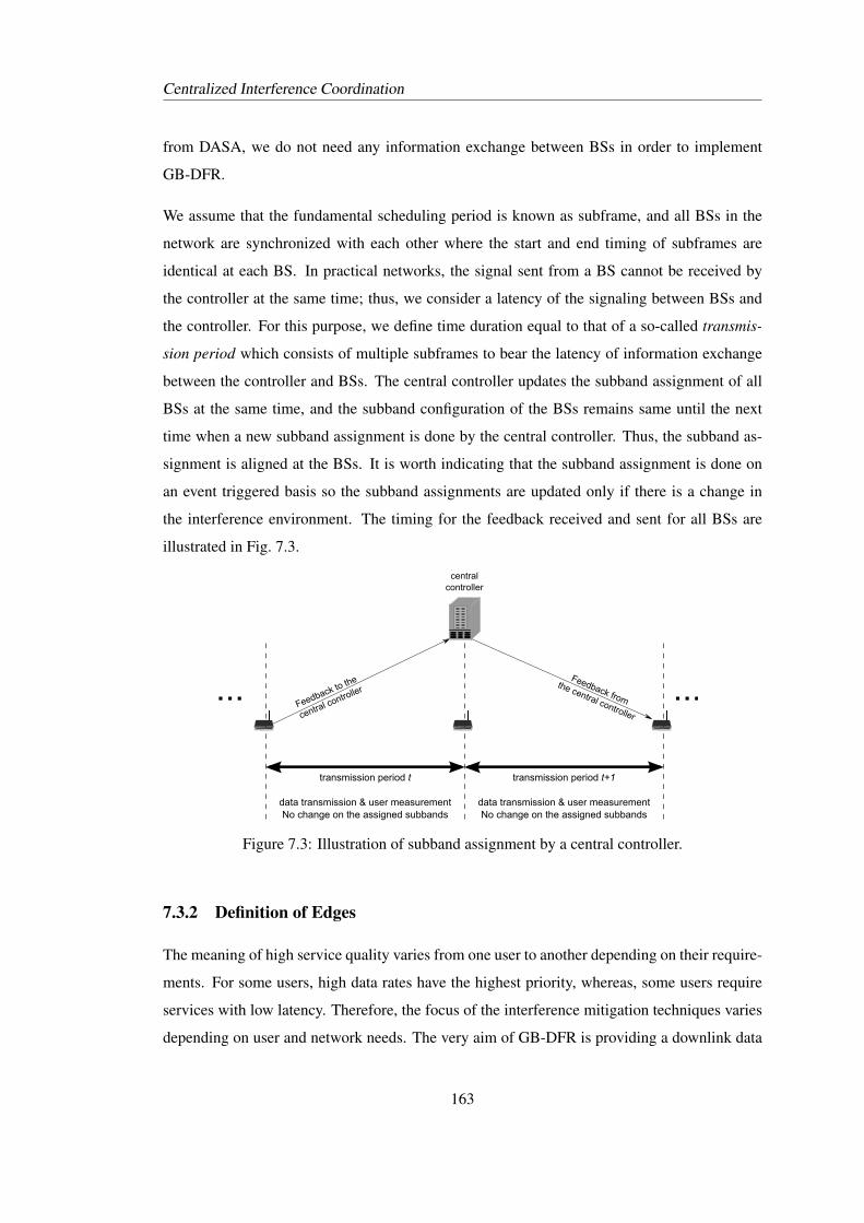
Centralized Interference Coordination
from DASA, we do not need any information exchange between BSs in order to implement
GB-DFR.
We assume that the fundamental scheduling period is known as subframe, and all BSs in the
network are synchronized with each other where the start and end timing of subframes are
identical at each BS. In practical networks, the signal sent from a BS cannot be received by
the controller at the same time; thus, we consider a latency of the signaling between BSs and
the controller. For this purpose, we define time duration equal to that of a so-called transmis-
sion period which consists of multiple subframes to bear the latency of information exchange
between the controller and BSs. The central controller updates the subband assignment of all
BSs at the same time, and the subband configuration of the BSs remains same until the next
time when a new subband assignment is done by the central controller. Thus, the subband as-
signment is aligned at the BSs. It is worth indicating that the subband assignment is done on
an event triggered basis so the subband assignments are updated only if there is a change in
the interference environment. The timing for the feedback received and sent for all BSs are
illustrated in Fig. 7.3.
transmission period t
data transmission & user measurementNo change on the assigned subbands
Feedback to the
central controller
transmission period t+1
data transmission & user measurementNo change on the assigned subbands
Feedback from
the central controller
central controller
... ...
Figure 7.3: Illustration of subband assignment by a central controller.
7.3.2 Definition of Edges
The meaning of high service quality varies from one user to another depending on their require-
ments. For some users, high data rates have the highest priority, whereas, some users require
services with low latency. Therefore, the focus of the interference mitigation techniques varies
depending on user and network needs. The very aim of GB-DFR is providing a downlink data
163
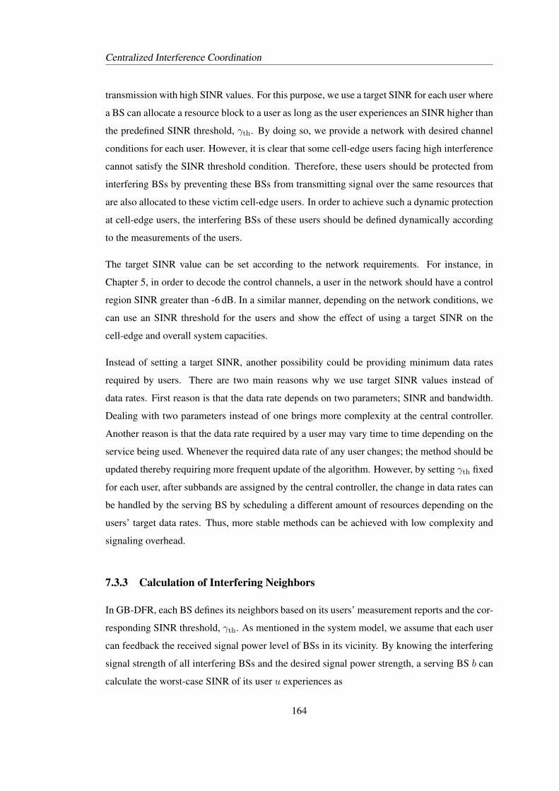
Centralized Interference Coordination
transmission with high SINR values. For this purpose, we use a target SINR for each user where
a BS can allocate a resource block to a user as long as the user experiences an SINR higher than
the predefined SINR threshold, γth. By doing so, we provide a network with desired channel
conditions for each user. However, it is clear that some cell-edge users facing high interference
cannot satisfy the SINR threshold condition. Therefore, these users should be protected from
interfering BSs by preventing these BSs from transmitting signal over the same resources that
are also allocated to these victim cell-edge users. In order to achieve such a dynamic protection
at cell-edge users, the interfering BSs of these users should be defined dynamically according
to the measurements of the users.
The target SINR value can be set according to the network requirements. For instance, in
Chapter 5, in order to decode the control channels, a user in the network should have a control
region SINR greater than -6 dB. In a similar manner, depending on the network conditions, we
can use an SINR threshold for the users and show the effect of using a target SINR on the
cell-edge and overall system capacities.
Instead of setting a target SINR, another possibility could be providing minimum data rates
required by users. There are two main reasons why we use target SINR values instead of
data rates. First reason is that the data rate depends on two parameters; SINR and bandwidth.
Dealing with two parameters instead of one brings more complexity at the central controller.
Another reason is that the data rate required by a user may vary time to time depending on the
service being used. Whenever the required data rate of any user changes; the method should be
updated thereby requiring more frequent update of the algorithm. However, by setting γth fixed
for each user, after subbands are assigned by the central controller, the change in data rates can
be handled by the serving BS by scheduling a different amount of resources depending on the
users’ target data rates. Thus, more stable methods can be achieved with low complexity and
signaling overhead.
7.3.3 Calculation of Interfering Neighbors
In GB-DFR, each BS defines its neighbors based on its users’ measurement reports and the cor-
responding SINR threshold, γth. As mentioned in the system model, we assume that each user
can feedback the received signal power level of BSs in its vicinity. By knowing the interfering
signal strength of all interfering BSs and the desired signal power strength, a serving BS b can
calculate the worst-case SINR of its user u experiences as
164
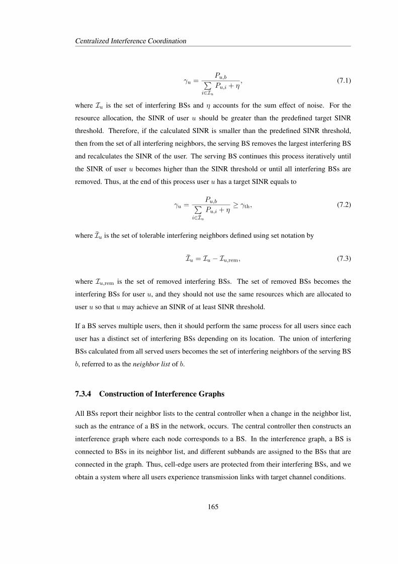
Centralized Interference Coordination
γu =Pu,b∑
i∈IuPu,i + η
, (7.1)
where Iu is the set of interfering BSs and η accounts for the sum effect of noise. For the
resource allocation, the SINR of user u should be greater than the predefined target SINR
threshold. Therefore, if the calculated SINR is smaller than the predefined SINR threshold,
then from the set of all interfering neighbors, the serving BS removes the largest interfering BS
and recalculates the SINR of the user. The serving BS continues this process iteratively until
the SINR of user u becomes higher than the SINR threshold or until all interfering BSs are
removed. Thus, at the end of this process user u has a target SINR equals to
γu =Pu,b∑
i∈IuPu,i + η
≥ γth, (7.2)
where Iu is the set of tolerable interfering neighbors defined using set notation by
Iu = Iu − Iu,rem, (7.3)
where Iu,rem is the set of removed interfering BSs. The set of removed BSs becomes the
interfering BSs for user u, and they should not use the same resources which are allocated to
user u so that u may achieve an SINR of at least SINR threshold.
If a BS serves multiple users, then it should perform the same process for all users since each
user has a distinct set of interfering BSs depending on its location. The union of interfering
BSs calculated from all served users becomes the set of interfering neighbors of the serving BS
b, referred to as the neighbor list of b.
7.3.4 Construction of Interference Graphs
All BSs report their neighbor lists to the central controller when a change in the neighbor list,
such as the entrance of a BS in the network, occurs. The central controller then constructs an
interference graph where each node corresponds to a BS. In the interference graph, a BS is
connected to BSs in its neighbor list, and different subbands are assigned to the BSs that are
connected in the graph. Thus, cell-edge users are protected from their interfering BSs, and we
obtain a system where all users experience transmission links with target channel conditions.
165
Centralized Interference Coordination
Central Cont roller
A
B
C
D
Corresponding Interference Graph
Feedback from BS to the controllerFeedback from user to the serving BSHigh interference that should be mitigated
2
1
3
5
4
A
B
D
CB,C,D D
Figure 7.4: Construction of an interference graph at the central controller.
The construction of the interference graph at the central controller is illustrated in Fig. 7.4.
According to the figure, each user in the network reports the received signal power strength of
the BSs in its vicinity. Based on the measurement reports, each BS calculates its own neighbor
list. For instance, user 1 in cell A faces high interference from BSs B and D and user 2 receives
strong interference from BS C. Therefore, in the neighbor list of BS A, there are BSs B, C and
D which are the union set of interfering BSs of user 1 and user 2. Similarly, BS D is listed
in the neighbor list of BS C as user 5 served by BS C suffers severe interference from BS D.
As shown in the figure, BSs report their own neighboring lists to the central controller and the
controller builds the corresponding interference graph. One important point here is that if BS A
reports BS B as its neighbor, then BS B automatically becomes the neighbor of BS A, whether
BS B reports BS A as its neighbor or not. For instance, in Fig. 7.4, although, BS B and D do
not have any interfering neighbors; they are connected to BS A in the interference graph since
user 1 served by BS A faces high interference from them.
A similar interference graph construction procedure is adopted in [121,123,124], but the neigh-
boring relations are constructed between users meaning each node represents a user in the in-
terference graph. In this case, the central controller gets all measurement reports of users and
calculates the interfering BSs for each user according to (5.6). Then, in the interference graph,
a given user is connected to all users served by the interfering BSs. The effect of applying
GB-DFR with the BS-based and user-based interference graphs in terms of signaling overhead
and performance will be discussed in the next section when we explain GB-DFR with the user-
based interference graph.
166
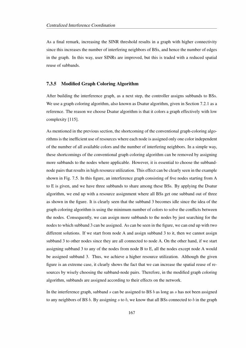
Centralized Interference Coordination
As a final remark, increasing the SINR threshold results in a graph with higher connectivity
since this increases the number of interfering neighbors of BSs, and hence the number of edges
in the graph. In this way, user SINRs are improved, but this is traded with a reduced spatial
reuse of subbands.
7.3.5 Modified Graph Coloring Algorithm
After building the interference graph, as a next step, the controller assigns subbands to BSs.
We use a graph coloring algorithm, also known as Dsatur algorithm, given in Section 7.2.1 as a
reference. The reason we choose Dsatur algorithm is that it colors a graph effectively with low
complexity [115].
As mentioned in the previous section, the shortcoming of the conventional graph-coloring algo-
rithms is the inefficient use of resources where each node is assigned only one color independent
of the number of all available colors and the number of interfering neighbors. In a simple way,
these shortcomings of the conventional graph coloring algorithm can be removed by assigning
more subbands to the nodes where applicable. However, it is essential to choose the subband-
node pairs that results in high resource utilization. This effect can be clearly seen in the example
shown in Fig. 7.5. In this figure, an interference graph consisting of five nodes starting from A
to E is given, and we have three subbands to share among these BSs. By applying the Dsatur
algorithm, we end up with a resource assignment where all BSs get one subband out of three
as shown in the figure. It is clearly seen that the subband 3 becomes idle since the idea of the
graph coloring algorithm is using the minimum number of colors to solve the conflicts between
the nodes. Consequently, we can assign more subbands to the nodes by just searching for the
nodes to which subband 3 can be assigned. As can be seen in the figure, we can end up with two
different solutions. If we start from node A and assign subband 3 to it, then we cannot assign
subband 3 to other nodes since they are all connected to node A. On the other hand, if we start
assigning subband 3 to any of the nodes from node B to E, all the nodes except node A would
be assigned subband 3. Thus, we achieve a higher resource utilization. Although the given
figure is an extreme case, it clearly shows the fact that we can increase the spatial reuse of re-
sources by wisely choosing the subband-node pairs. Therefore, in the modified graph coloring
algorithm, subbands are assigned according to their effects on the network.
In the interference graph, subband s can be assigned to BS b as long as s has not been assigned
to any neighbors of BS b. By assigning s to b, we know that all BSs connected to b in the graph
167
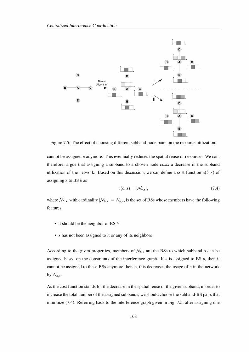
Centralized Interference Coordination
AB C
D
E II
AB C
D
E
AB C
D
E
AB C
D
E
IDsaturAlgorithm
Figure 7.5: The effect of choosing different subband-node pairs on the resource utilization.
cannot be assigned s anymore. This eventually reduces the spatial reuse of resources. We can,
therefore, argue that assigning a subband to a chosen node costs a decrease in the subband
utilization of the network. Based on this discussion, we can define a cost function c(b, s) of
assigning s to BS b as
c(b, s) = |Nb,s|, (7.4)
whereNb,s, with cardinality |Nb,s| = Nb,s, is the set of BSs whose members have the following
features:
• it should be the neighbor of BS b
• s has not been assigned to it or any of its neighbors
According to the given properties, members of Nb,s are the BSs to which subband s can be
assigned based on the constraints of the interference graph. If s is assigned to BS b, then it
cannot be assigned to these BSs anymore; hence, this decreases the usage of s in the network
by Nb,s.
As the cost function stands for the decrease in the spatial reuse of the given subband, in order to
increase the total number of the assigned subbands, we should choose the subband-BS pairs that
minimize (7.4). Referring back to the interference graph given in Fig. 7.5, after assigning one
168
Centralized Interference Coordination
subband to each node, the cost of assigning subband 3 to node A is 4 since it has 4 neighbors to
which subband 3 can be assigned. On the other hand, the cost of assigning subband 3 to nodes
B, C, D and E is 1. Thus, assigning subband 3 to one of these nodes instead of node A increases
the spatial reuse of resources.
Based on the cost function, we develop a modified graph coloring algorithm where subbands
are assigned to BSs in two steps that are explained in the following sections.
7.3.5.1 Step-1
In the first step of GB-DFR, subbands are assigned to BSs by using the conventional graph
coloring algorithm with some extensions where for each BS, the subband s that minimizes the
cost function (7.4) is selected. Thus, more subbands can be allocated within the network.
Additionally, another novelty introduced with GB-DFR is that we use a design parameter smin.
The parameter smin stands for the minimum number of subbands that should be assigned to
each BS. With smin, the minimum frequency bandwidth assigned to a BS is adapted. The
use of smin is particularly beneficial when the total number of subbands, NS, is large. This
is achieved by applying the modified graph coloring algorithm to each BS smin times. In this
way, we increase the fairness among BSs in terms of the number of assigned subbands. smin
can also be set for each BS separately depending on the data requirements. For instance, if a
BS is required to serve a large number of users with high data rates, then smin for this BS could
be set larger than other BSs.
The pseudo code of the corresponding algorithm is given in the following, where S denotes the
pool of all subbands, and the saturation degree of a BS indicates the total number of different
subbands that are assigned to this BS’s neighbors. Also, the term available subbands stands
for the set of subbands that can be assigned (i.e. that are available for an assignment) to a BS
without causing any conflict in the interference graph. In other words, available subbands of a
given BS are the set of subbands that are not assigned to the neighbors of the given BS in the
interference graph. Furthermore, for the sake of simplicity, we set smin the same for all BSs,
however, as indicated previously, it can be set differently at each BS depending on the traffic
conditions.
1: define a pool of subbands, S as [1, 2, .., NS]
2: for i = 1 to smin do
169
Centralized Interference Coordination
3: mark all BSs as unselected
4: repeat
5: sort all unselected BSs by decreasing order of saturation degree:
i select the BS having the maximum saturation degree
ii if there are BSs having same saturation degrees then among these BSs select the
BS having the maximum number of unselected neighbors
6: find out the available subband(s) Sav that can be assigned to the selected BS b
i if there are available subbands: among the available subbands, assign the one
with the minimum cost function value: s = arg mins∈Sav
{c(b, s)}.
ii if there is no available subband: among all subbands in the pool that are not
assigned to BS b, choose the one having the minimum cost function value
7:
8: until all BSs are selected once
9: end for
In the algorithm, the selection procedure of BSs is same as the Dsatur algorithm. The difference
is choosing the subband for the selected BS. We first find out the set of subbands that are
not assigned to the neighbors of the selected BS (i.e. available subbands for the selected BS).
Among these subbands, then, we choose the one which leads to the minimum cost to a network.
In some situations, it is possible that, for a selected BS, there is no available subband that can be
assigned without causing a conflict in the graph. Such situations can happen when the number
of subbands is smaller than the required number of colors to color the graph (for instance in
dense deployments or if smin is set to a high value). For such users, among all subbands, we
choose the one that having the minimum cost function value. By doing so, we decrease the
number of potential interfering neighbors that use the same subband.
7.3.5.2 Step-2
After assigning each BS smin subbands, the second step of GB-DFR searches if there exists
some BSs to which more subbands can be assigned. For this purpose, the algorithm of Step 2
iterates over all subbands. For each subband, the available BSs (to which the selected subband
170
Centralized Interference Coordination
can be assigned without causing any conflict in the graph) are identified. Then, among these
available BSs, the one with the minimum cost in (7.4) is selected. In this way, more subbands
can be allocated within the network improving the spatial reuse of the subbands. The algorithm
of Step 2 is detailed in the following pseudo code.
1: for s = 1 to NS do
2: repeat
3: identify available BSs, Bav, that s can be assigned to
4: for s and Bav:
i among Bav, assign s to BS b which provides b = arg minb∈Bav
{c(b, s)}
ii if more than one BS minimize the cost function, then assign s to the one having
minimum number of already assigned subbands
5: until s cannot be assigned to any BS further
6: end for
Step 2 of GB-DFR aims for high resource utilization where BSs facing low interference are
assigned more subbands. On the other hand, during Step 2, BSs having a large number of
neighbors in the interference graph are less likely assigned any subband. Therefore, it is clear
that we can achieve higher subband utilization by decreasing smin.
In case there are a large number of available subbands, plenty of resources are assigned to BSs
having favorable interference conditions, whereas the remaining BSs are only allocated a small
fraction of resources. Thus, although we choose non-optimum subband-BS pairs in terms of the
cost values, with the smin condition, we assign all BSs at least smin subbands that allows a fair
distribution of subbands in terms of the amount of resources assigned to BSs. Consequently, the
trade-off between the fair distribution of resources among BSs and the high resource utilization
should be taken into account depending on the network needs.
7.3.6 Simulation Setup and Results
In this section, we discuss the performance of GB-DFR in single-user scenarios where each
closed-access femto-BS serves only one user that is located in the same apartment.
171
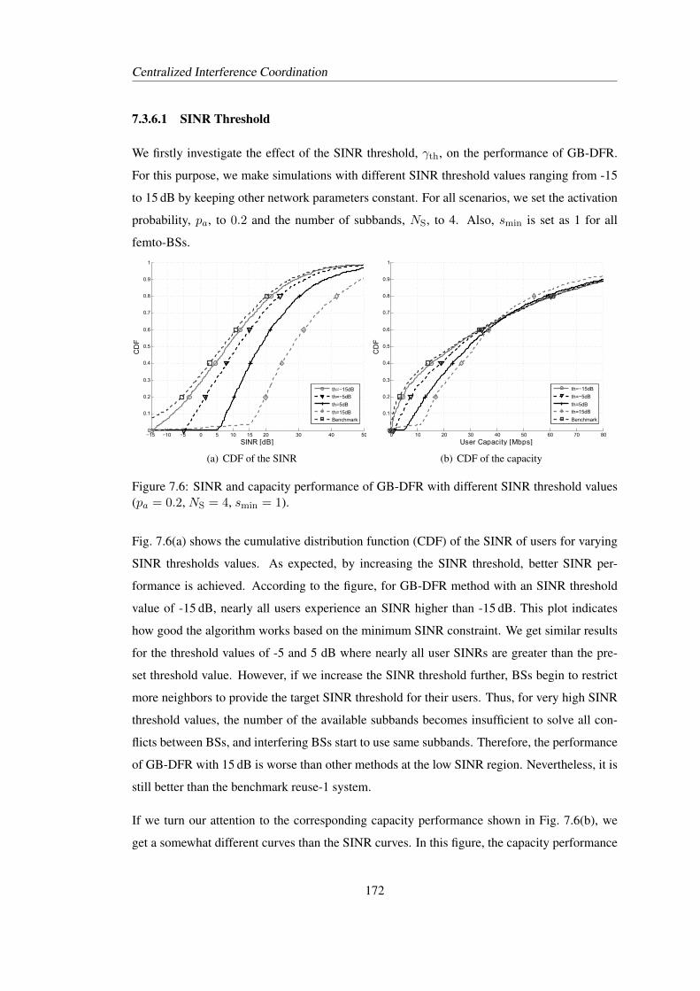
Centralized Interference Coordination
7.3.6.1 SINR Threshold
We firstly investigate the effect of the SINR threshold, γth, on the performance of GB-DFR.
For this purpose, we make simulations with different SINR threshold values ranging from -15
to 15 dB by keeping other network parameters constant. For all scenarios, we set the activation
probability, pa, to 0.2 and the number of subbands, NS, to 4. Also, smin is set as 1 for all
femto-BSs.
−15 −10 −5 0 5 10 15 20 30 40 500
0.1
0.2
0.3
0.4
0.5
0.6
0.7
0.8
0.9
1
SINRr[dB]
CD
F
th=−15dB
th=−5dB
th=5dB
th=15dB
Benchmark
(a) CDF of the SINR
0 10 20 30 40 50 60 70 800
0.1
0.2
0.3
0.4
0.5
0.6
0.7
0.8
0.9
1
UserdCapacityd[Mbps]
CD
F
th=−15dB
th=−5dB
th=5dB
th=15dB
Benchmark
(b) CDF of the capacity
Figure 7.6: SINR and capacity performance of GB-DFR with different SINR threshold values(pa = 0.2, NS = 4, smin = 1).
Fig. 7.6(a) shows the cumulative distribution function (CDF) of the SINR of users for varying
SINR thresholds values. As expected, by increasing the SINR threshold, better SINR per-
formance is achieved. According to the figure, for GB-DFR method with an SINR threshold
value of -15 dB, nearly all users experience an SINR higher than -15 dB. This plot indicates
how good the algorithm works based on the minimum SINR constraint. We get similar results
for the threshold values of -5 and 5 dB where nearly all user SINRs are greater than the pre-
set threshold value. However, if we increase the SINR threshold further, BSs begin to restrict
more neighbors to provide the target SINR threshold for their users. Thus, for very high SINR
threshold values, the number of the available subbands becomes insufficient to solve all con-
flicts between BSs, and interfering BSs start to use same subbands. Therefore, the performance
of GB-DFR with 15 dB is worse than other methods at the low SINR region. Nevertheless, it is
still better than the benchmark reuse-1 system.
If we turn our attention to the corresponding capacity performance shown in Fig. 7.6(b), we
get a somewhat different curves than the SINR curves. In this figure, the capacity performance
172
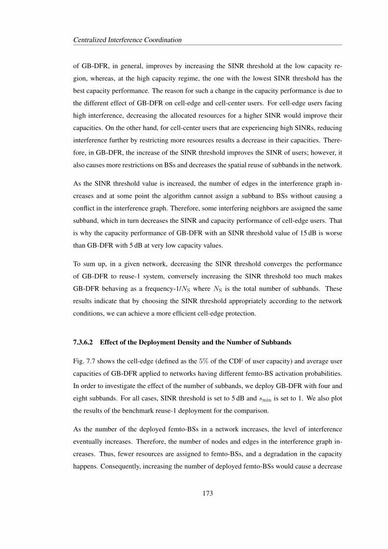
Centralized Interference Coordination
of GB-DFR, in general, improves by increasing the SINR threshold at the low capacity re-
gion, whereas, at the high capacity regime, the one with the lowest SINR threshold has the
best capacity performance. The reason for such a change in the capacity performance is due to
the different effect of GB-DFR on cell-edge and cell-center users. For cell-edge users facing
high interference, decreasing the allocated resources for a higher SINR would improve their
capacities. On the other hand, for cell-center users that are experiencing high SINRs, reducing
interference further by restricting more resources results a decrease in their capacities. There-
fore, in GB-DFR, the increase of the SINR threshold improves the SINR of users; however, it
also causes more restrictions on BSs and decreases the spatial reuse of subbands in the network.
As the SINR threshold value is increased, the number of edges in the interference graph in-
creases and at some point the algorithm cannot assign a subband to BSs without causing a
conflict in the interference graph. Therefore, some interfering neighbors are assigned the same
subband, which in turn decreases the SINR and capacity performance of cell-edge users. That
is why the capacity performance of GB-DFR with an SINR threshold value of 15 dB is worse
than GB-DFR with 5 dB at very low capacity values.
To sum up, in a given network, decreasing the SINR threshold converges the performance
of GB-DFR to reuse-1 system, conversely increasing the SINR threshold too much makes
GB-DFR behaving as a frequency-1/NS where NS is the total number of subbands. These
results indicate that by choosing the SINR threshold appropriately according to the network
conditions, we can achieve a more efficient cell-edge protection.
7.3.6.2 Effect of the Deployment Density and the Number of Subbands
Fig. 7.7 shows the cell-edge (defined as the 5% of the CDF of user capacity) and average user
capacities of GB-DFR applied to networks having different femto-BS activation probabilities.
In order to investigate the effect of the number of subbands, we deploy GB-DFR with four and
eight subbands. For all cases, SINR threshold is set to 5 dB and smin is set to 1. We also plot
the results of the benchmark reuse-1 deployment for the comparison.
As the number of the deployed femto-BSs in a network increases, the level of interference
eventually increases. Therefore, the number of nodes and edges in the interference graph in-
creases. Thus, fewer resources are assigned to femto-BSs, and a degradation in the capacity
happens. Consequently, increasing the number of deployed femto-BSs would cause a decrease
173
Centralized Interference Coordination
0.2 0.3 0.4 0.5 0.6 0.7 0.8 0.9 10
1
2
3
4
5
6
7
Femto−BSdactivationdprobability
Cel
l−E
dg
edC
apac
ityd
[Mb
ps]
BenchmarkGB−DFRdG4dsubbandsDGB−DFRdG8dsubbandsD
(a) Cell-edge capacity
0)2 0)3 0)4 0)5 0)6 0)7 0)8 0)9 15
10
15
20
25
30
35
40
Femto−BSUactivationUprobability
Ave
rag
eUU
serU
Cap
acit
yU[M
bp
s]
BenchmarkGB−DFRUG4UsubbandsDGB−DFRUG8UsubbandsD
(b) Average user capacity
Figure 7.7: Cell-edge and average user capacity values achieved with GB-DFR at differentnetwork deployments (γth = 5 dB, smin = 1).
on the performance of GB-DFR. Nevertheless, as can be seen in the figures, for all densities,
we achieve a better cell-edge performance with respect to the benchmark system that indicates
the effectiveness of GB-DFR in terms of the cell-edge performance.
According to the figures, increasing the number of subbands results a higher capacity perfor-
mance because the central controller has more choices to assign subbands. When we divide
the spectrum into more subbands, the ratio of the protected subband to the whole bandwidth
decreases. Thus, a small amount of resources are assigned during step-1 of GB-DFR; however,
the amount of resources that can be allocated to BSs during step-2 increases. Hence, both re-
source utilization and capacity increase. Furthermore, cell-edge users are provided resources
with an SINR greater than the threshold, as long as the number of the subbands is enough to
solve all conflicts in the interference graph. In the case of the dense deployment of femto-
BSs, the size of the interference graph increases, thus, applying GB-DFR with a large number
of subbands would be enough to assign different subbands at interfering BSs connected with
edges in the interference graph. On the other hand, if the number of available subbands is low,
interfering BSs could be assigned the same subband; thus, they cause high interference to each
other. Therefore, the performance of GB-DFR with eight subbands is better than GB-DFR with
four subbands in general.
The only exception occurs at scenarios where femto-BSs are deployed with a low density. As
using more subbands leads to an improvement in the resource utilization, it also decreases the
amount of resources that are reserved for cell-edge users. Thus, GB-DFR with four subbands
174
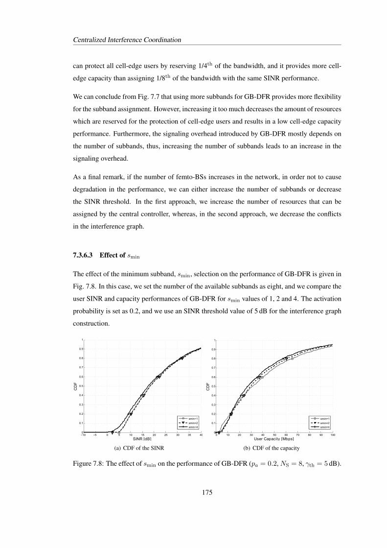
Centralized Interference Coordination
can protect all cell-edge users by reserving 1/4th of the bandwidth, and it provides more cell-
edge capacity than assigning 1/8th of the bandwidth with the same SINR performance.
We can conclude from Fig. 7.7 that using more subbands for GB-DFR provides more flexibility
for the subband assignment. However, increasing it too much decreases the amount of resources
which are reserved for the protection of cell-edge users and results in a low cell-edge capacity
performance. Furthermore, the signaling overhead introduced by GB-DFR mostly depends on
the number of subbands, thus, increasing the number of subbands leads to an increase in the
signaling overhead.
As a final remark, if the number of femto-BSs increases in the network, in order not to cause
degradation in the performance, we can either increase the number of subbands or decrease
the SINR threshold. In the first approach, we increase the number of resources that can be
assigned by the central controller, whereas, in the second approach, we decrease the conflicts
in the interference graph.
7.3.6.3 Effect of smin
The effect of the minimum subband, smin, selection on the performance of GB-DFR is given in
Fig. 7.8. In this case, we set the number of the available subbands as eight, and we compare the
user SINR and capacity performances of GB-DFR for smin values of 1, 2 and 4. The activation
probability is set as 0.2, and we use an SINR threshold value of 5 dB for the interference graph
construction.
−10 −5 0 5 10 15 20 25 30 35 400
0.1
0.2
0.3
0.4
0.5
0.6
0.7
0.8
0.9
1
SINR [dB]
CD
F
smin=1
smin=2
smin=4
(a) CDF of the SINR
0 10 20 30 40 50 60 70 80 90 1000
0.1
0.2
0.3
0.4
0.5
0.6
0.7
0.8
0.9
1
User=Capacity=[Mbps]
CD
F
smin=1
smin=2
smin=4
(b) CDF of the capacity
Figure 7.8: The effect of smin on the performance of GB-DFR (pa = 0.2,NS = 8, γth = 5 dB).
175
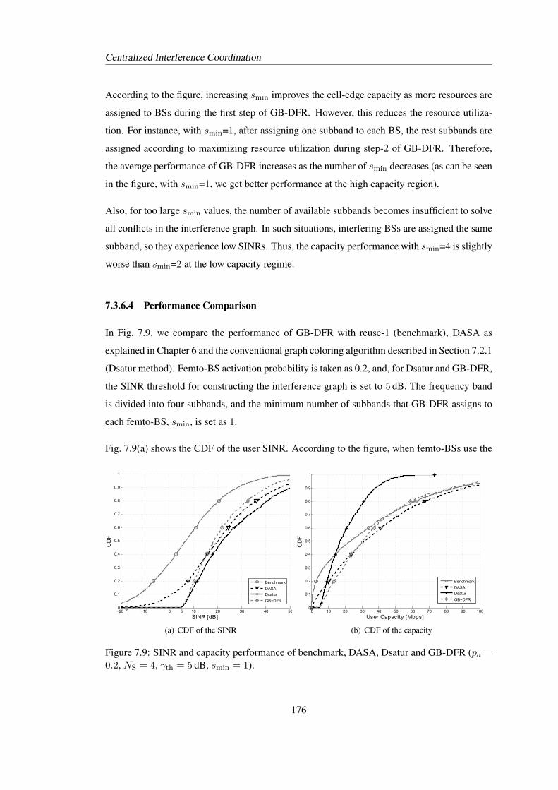
Centralized Interference Coordination
According to the figure, increasing smin improves the cell-edge capacity as more resources are
assigned to BSs during the first step of GB-DFR. However, this reduces the resource utiliza-
tion. For instance, with smin=1, after assigning one subband to each BS, the rest subbands are
assigned according to maximizing resource utilization during step-2 of GB-DFR. Therefore,
the average performance of GB-DFR increases as the number of smin decreases (as can be seen
in the figure, with smin=1, we get better performance at the high capacity region).
Also, for too large smin values, the number of available subbands becomes insufficient to solve
all conflicts in the interference graph. In such situations, interfering BSs are assigned the same
subband, so they experience low SINRs. Thus, the capacity performance with smin=4 is slightly
worse than smin=2 at the low capacity regime.
7.3.6.4 Performance Comparison
In Fig. 7.9, we compare the performance of GB-DFR with reuse-1 (benchmark), DASA as
explained in Chapter 6 and the conventional graph coloring algorithm described in Section 7.2.1
(Dsatur method). Femto-BS activation probability is taken as 0.2, and, for Dsatur and GB-DFR,
the SINR threshold for constructing the interference graph is set to 5 dB. The frequency band
is divided into four subbands, and the minimum number of subbands that GB-DFR assigns to
each femto-BS, smin, is set as 1.
Fig. 7.9(a) shows the CDF of the user SINR. According to the figure, when femto-BSs use the
−20 −10 0 5 10 20 30 40 500
0.1
0.2
0.3
0.4
0.5
0.6
0.7
0.8
0.9
1
SINRA[dB]
CD
F
Benchmark
DASA
Dsatur
GB−DFR
(a) CDF of the SINR
0 10 20 30 40 50 60 70 80 90 1000
0.1
0.2
0.3
0.4
0.5
0.6
0.7
0.8
0.9
1
UserhCapacityh[Mbps]
CD
F
Benchmark
DASA
Dsatur
GB−DFR
(b) CDF of the capacity
Figure 7.9: SINR and capacity performance of benchmark, DASA, Dsatur and GB-DFR (pa =0.2, NS = 4, γth = 5 dB, smin = 1).
176
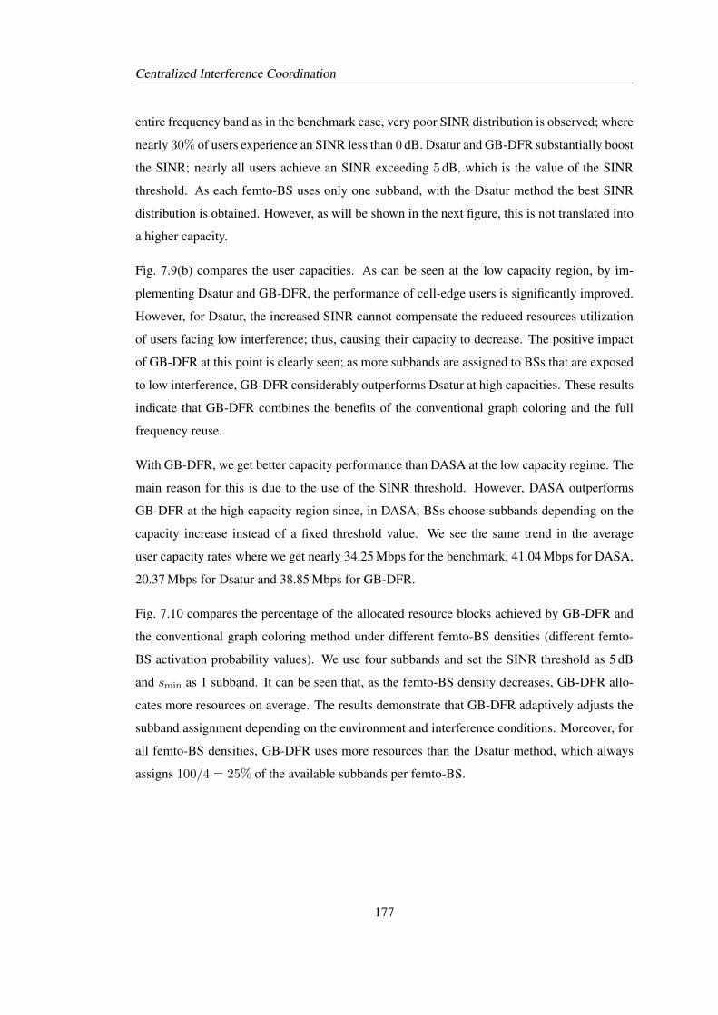
Centralized Interference Coordination
entire frequency band as in the benchmark case, very poor SINR distribution is observed; where
nearly 30% of users experience an SINR less than 0 dB. Dsatur and GB-DFR substantially boost
the SINR; nearly all users achieve an SINR exceeding 5 dB, which is the value of the SINR
threshold. As each femto-BS uses only one subband, with the Dsatur method the best SINR
distribution is obtained. However, as will be shown in the next figure, this is not translated into
a higher capacity.
Fig. 7.9(b) compares the user capacities. As can be seen at the low capacity region, by im-
plementing Dsatur and GB-DFR, the performance of cell-edge users is significantly improved.
However, for Dsatur, the increased SINR cannot compensate the reduced resources utilization
of users facing low interference; thus, causing their capacity to decrease. The positive impact
of GB-DFR at this point is clearly seen; as more subbands are assigned to BSs that are exposed
to low interference, GB-DFR considerably outperforms Dsatur at high capacities. These results
indicate that GB-DFR combines the benefits of the conventional graph coloring and the full
frequency reuse.
With GB-DFR, we get better capacity performance than DASA at the low capacity regime. The
main reason for this is due to the use of the SINR threshold. However, DASA outperforms
GB-DFR at the high capacity region since, in DASA, BSs choose subbands depending on the
capacity increase instead of a fixed threshold value. We see the same trend in the average
user capacity rates where we get nearly 34.25 Mbps for the benchmark, 41.04 Mbps for DASA,
20.37 Mbps for Dsatur and 38.85 Mbps for GB-DFR.
Fig. 7.10 compares the percentage of the allocated resource blocks achieved by GB-DFR and
the conventional graph coloring method under different femto-BS densities (different femto-
BS activation probability values). We use four subbands and set the SINR threshold as 5 dB
and smin as 1 subband. It can be seen that, as the femto-BS density decreases, GB-DFR allo-
cates more resources on average. The results demonstrate that GB-DFR adaptively adjusts the
subband assignment depending on the environment and interference conditions. Moreover, for
all femto-BS densities, GB-DFR uses more resources than the Dsatur method, which always
assigns 100/4 = 25% of the available subbands per femto-BS.
177
Centralized Interference Coordination
0.2 0.3 0.4 0.5 0.6 0.7 0.8 0.9 120
25
30
35
40
45
50
55
60
65
70
Femto−BSuactivationuprobability
Res
ou
rceu
Uti
lizat
ion
uPer
cen
tag
e
GB−DFR
Dsatur
Figure 7.10: Resource utilization with respect to varying femtocell deployment densities (NS =4, γth = 5 dB, smin = 1).
7.3.6.5 Effect of the Chromatic Number
The chromatic number of a generated graph indicates the minimum number of subbands re-
quired to achieve a resource assignment without causing any conflict in the given graph (i.e. BSs
that are connected in the graph are assigned different subbands). We know that the chromatic
number of a graph is directly related with the SINR threshold. By increasing the SINR thresh-
old, more BSs in the graph are connected to each other, and the chromatic number of the graph
increases. Similarly, by decreasing the SINR threshold, we can obtain an interference graph
with a low chromatic number.
Until now, we have shown the performance of the conventional graph coloring algorithm (Dsatur)
and GB-DFR where the interference graph is generated based on a preset SINR threshold. In
this section, we investigate the effect of the chromatic number of a generated interference graph
and discuss the relation between the number of subbands and BSs and the chromatic number
on the performance of Dsatur and GB-DFR under different scenarios. We use the BS-based
interference graphs, however, the same findings are also valid for the user-based interference
graphs. Furthermore, for GB-DFR, we assume that the minimum subband, smin, per BS is one.
Using smin different than one would only increase the chromatic number of the generated inter-
ference graph, but it does not affect the relation between the chromatic number and the number
of subbands.
With the Dsatur method, each BS in the graph is assigned only one subband irrespective of
the interfering environment. As we discussed in Section 7.2.2, if the chromatic number of the
generated interference graph equals to NC, then the central controller assigns NC subbands to
178
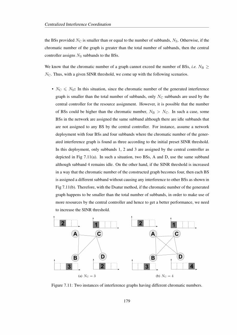
Centralized Interference Coordination
the BSs provided NC is smaller than or equal to the number of subbands, NS. Otherwise, if the
chromatic number of the graph is greater than the total number of subbands, then the central
controller assigns NS subbands to the BSs.
We know that the chromatic number of a graph cannot exceed the number of BSs, i.e. NB ≥
NC. Thus, with a given SINR threshold, we come up with the following scenarios.
• NC 6 NS: In this situation, since the chromatic number of the generated interference
graph is smaller than the total number of subbands, only NC subbands are used by the
central controller for the resource assignment. However, it is possible that the number
of BSs could be higher than the chromatic number, NB > NC. In such a case, some
BSs in the network are assigned the same subband although there are idle subbands that
are not assigned to any BS by the central controller. For instance, assume a network
deployment with four BSs and four subbands where the chromatic number of the gener-
ated interference graph is found as three according to the initial preset SINR threshold.
In this deployment, only subbands 1, 2 and 3 are assigned by the central controller as
depicted in Fig 7.11(a). In such a situation, two BSs, A and D, use the same subband
although subband 4 remains idle. On the other hand, if the SINR threshold is increased
in a way that the chromatic number of the constructed graph becomes four, then each BS
is assigned a different subband without causing any interference to other BSs as shown in
Fig 7.11(b). Therefore, with the Dsatur method, if the chromatic number of the generated
graph happens to be smaller than the total number of subbands, in order to make use of
more resources by the central controller and hence to get a better performance, we need
to increase the SINR threshold.
A
B
C
D
2 1
3 2
(a) NC = 3
A
B
C
D
2 1
3 4
(b) NC = 4
Figure 7.11: Two instances of interference graphs having different chromatic numbers.
179
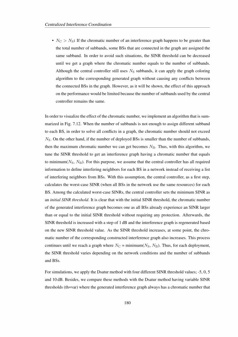
Centralized Interference Coordination
• NC > NS: If the chromatic number of an interference graph happens to be greater than
the total number of subbands, some BSs that are connected in the graph are assigned the
same subband. In order to avoid such situations, the SINR threshold can be decreased
until we get a graph where the chromatic number equals to the number of subbands.
Although the central controller still uses NS subbands, it can apply the graph coloring
algorithm to the corresponding generated graph without causing any conflicts between
the connected BSs in the graph. However, as it will be shown, the effect of this approach
on the performance would be limited because the number of subbands used by the central
controller remains the same.
In order to visualize the effect of the chromatic number, we implement an algorithm that is sum-
marized in Fig. 7.12. When the number of subbands is not enough to assign different subband
to each BS, in order to solve all conflicts in a graph, the chromatic number should not exceed
NS. On the other hand, if the number of deployed BSs is smaller than the number of subbands,
then the maximum chromatic number we can get becomes NB. Thus, with this algorithm, we
tune the SINR threshold to get an interference graph having a chromatic number that equals
to minimum(NS, NB). For this purpose, we assume that the central controller has all required
information to define interfering neighbors for each BS in a network instead of receiving a list
of interfering neighbors from BSs. With this assumption, the central controller, as a first step,
calculates the worst-case SINR (when all BSs in the network use the same resources) for each
BS. Among the calculated worst-case SINRs, the central controller sets the minimum SINR as
an initial SINR threshold. It is clear that with the initial SINR threshold, the chromatic number
of the generated interference graph becomes one as all BSs already experience an SINR larger
than or equal to the initial SINR threshold without requiring any protection. Afterwards, the
SINR threshold is increased with a step of 1 dB and the interference graph is regenerated based
on the new SINR threshold value. As the SINR threshold increases, at some point, the chro-
matic number of the corresponding constructed interference graph also increases. This process
continues until we reach a graph where NC = minimum(NS, NB). Thus, for each deployment,
the SINR threshold varies depending on the network conditions and the number of subbands
and BSs.
For simulations, we apply the Dsatur method with four different SINR threshold values; -5, 0, 5
and 10 dB. Besides, we compare these methods with the Dsatur method having variable SINR
thresholds (th=var) where the generated interference graph always has a chromatic number that
180
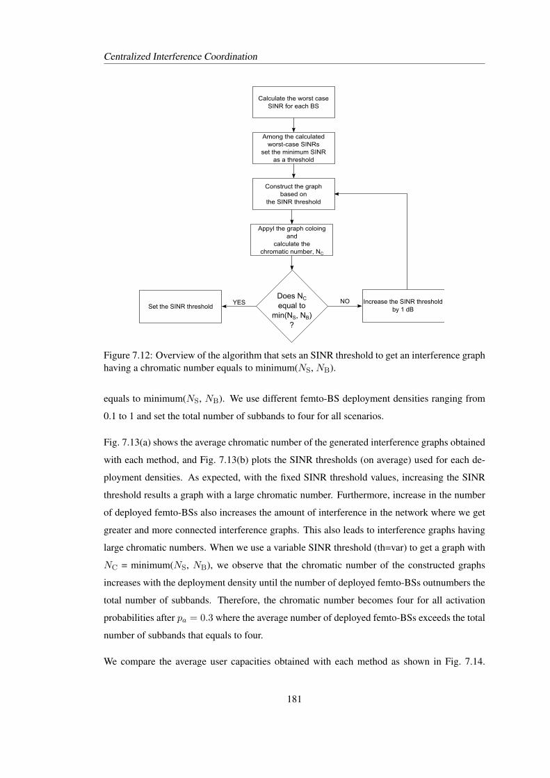
Centralized Interference Coordination
Calculate,the,worst,case,SINR,for,each,BS
Among,the,calculated,worst-case,SINRs
set,the,minimum,SINR,as,a,threshold
YESDoes,NC,equal,to
min(NS,,NB)?
Set,the,SINR,thresholdNO Increase,the,SINR,threshold,
by,1,dB
Construct,the,graph,based,on,
the,SINR,threshold
Appyl,the,graph,coloing,and,
calculate,the,chromatic,number,,NC
Figure 7.12: Overview of the algorithm that sets an SINR threshold to get an interference graphhaving a chromatic number equals to minimum(NS, NB).
equals to minimum(NS, NB). We use different femto-BS deployment densities ranging from
0.1 to 1 and set the total number of subbands to four for all scenarios.
Fig. 7.13(a) shows the average chromatic number of the generated interference graphs obtained
with each method, and Fig. 7.13(b) plots the SINR thresholds (on average) used for each de-
ployment densities. As expected, with the fixed SINR threshold values, increasing the SINR
threshold results a graph with a large chromatic number. Furthermore, increase in the number
of deployed femto-BSs also increases the amount of interference in the network where we get
greater and more connected interference graphs. This also leads to interference graphs having
large chromatic numbers. When we use a variable SINR threshold (th=var) to get a graph with
NC = minimum(NS, NB), we observe that the chromatic number of the constructed graphs
increases with the deployment density until the number of deployed femto-BSs outnumbers the
total number of subbands. Therefore, the chromatic number becomes four for all activation
probabilities after pa = 0.3 where the average number of deployed femto-BSs exceeds the total
number of subbands that equals to four.
We compare the average user capacities obtained with each method as shown in Fig. 7.14.
181
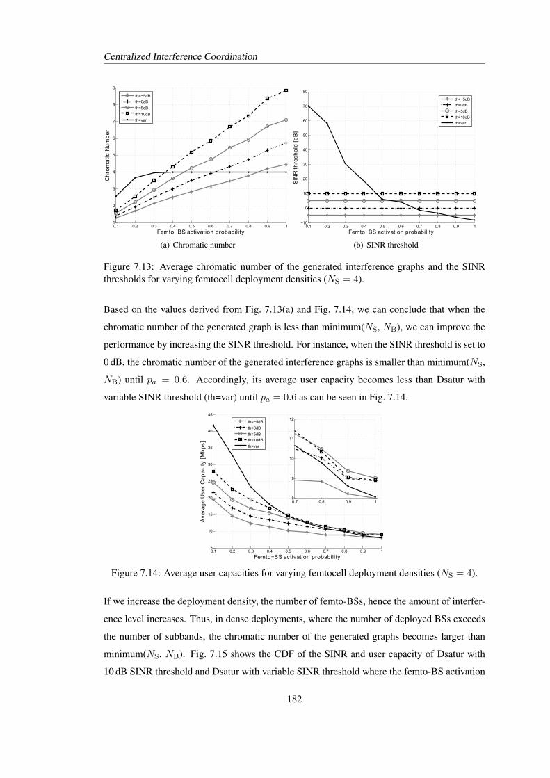
Centralized Interference Coordination
0.1 0.2 0.3 0.4 0.5 0.6 0.7 0.8 0.9 11
2
3
4
5
6
7
8
9
Femto−BSNactivationNprobability
Ch
rom
atic
NNu
mb
er
th=−5dB
th=0dB
th=5dB
th=10dB
th=var
(a) Chromatic number
0.1 0.2 0.3 0.4 0.5 0.6 0.7 0.8 0.9 1−10
0
10
20
30
40
50
60
70
80
Femto−BSRactivationRprobability
SIN
RRt
hre
sho
ldR[
dB
]
th=−5dB
th=0dB
th=5dB
th=10dB
th=var
(b) SINR threshold
Figure 7.13: Average chromatic number of the generated interference graphs and the SINRthresholds for varying femtocell deployment densities (NS = 4).
Based on the values derived from Fig. 7.13(a) and Fig. 7.14, we can conclude that when the
chromatic number of the generated graph is less than minimum(NS, NB), we can improve the
performance by increasing the SINR threshold. For instance, when the SINR threshold is set to
0 dB, the chromatic number of the generated interference graphs is smaller than minimum(NS,
NB) until pa = 0.6. Accordingly, its average user capacity becomes less than Dsatur with
variable SINR threshold (th=var) until pa = 0.6 as can be seen in Fig. 7.14.
0.1 0.2 0.3 0.4 0.5 0.6 0.7 0.8 0.9 15
10
15
20
25
30
35
40
45
Femto−BSUactivationUprobability
Ave
rag
eUU
serU
Cap
acit
yU[M
bp
s]
th=−5dB
th=0dB
th=5dB
th=10dB
th=var
0.7 0.8 0.9 18
9
10
11
12
Figure 7.14: Average user capacities for varying femtocell deployment densities (NS = 4).
If we increase the deployment density, the number of femto-BSs, hence the amount of interfer-
ence level increases. Thus, in dense deployments, where the number of deployed BSs exceeds
the number of subbands, the chromatic number of the generated graphs becomes larger than
minimum(NS, NB). Fig. 7.15 shows the CDF of the SINR and user capacity of Dsatur with
10 dB SINR threshold and Dsatur with variable SINR threshold where the femto-BS activation
182
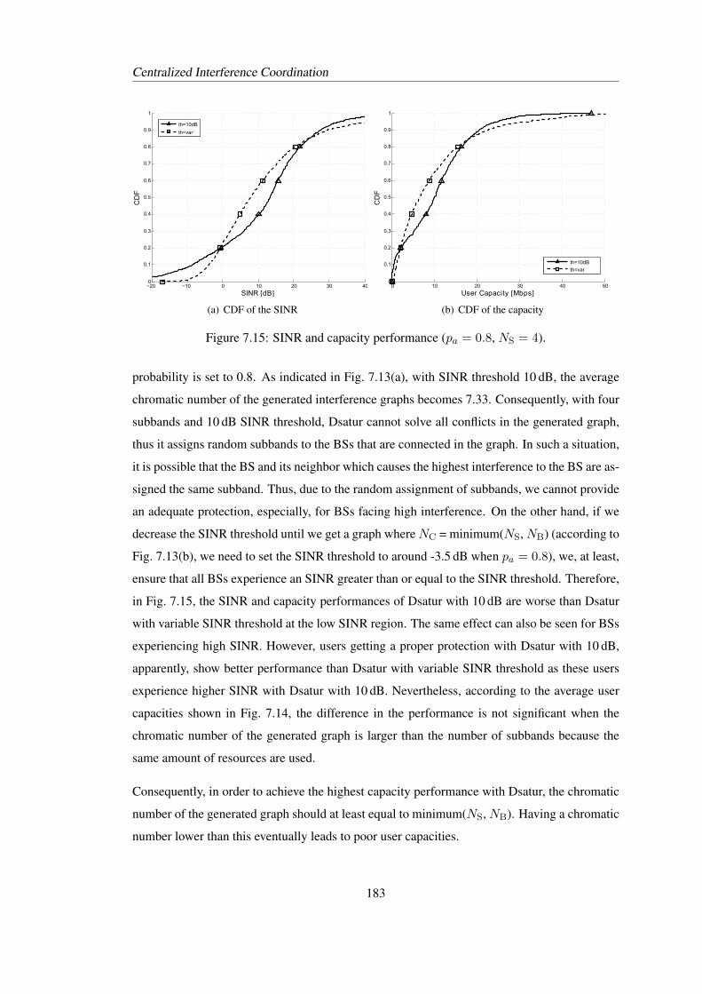
Centralized Interference Coordination
−20 −10 0 10 20 30 400
0.1
0.2
0.3
0.4
0.5
0.6
0.7
0.8
0.9
1
SINR [dB]
CD
F
th=10dB
th=var
(a) CDF of the SINR
0 10 20 30 40 500
0.1
0.2
0.3
0.4
0.5
0.6
0.7
0.8
0.9
1
UserdCapacityd[Mbps]
CD
F
th=10dB
th=var
(b) CDF of the capacity
Figure 7.15: SINR and capacity performance (pa = 0.8, NS = 4).
probability is set to 0.8. As indicated in Fig. 7.13(a), with SINR threshold 10 dB, the average
chromatic number of the generated interference graphs becomes 7.33. Consequently, with four
subbands and 10 dB SINR threshold, Dsatur cannot solve all conflicts in the generated graph,
thus it assigns random subbands to the BSs that are connected in the graph. In such a situation,
it is possible that the BS and its neighbor which causes the highest interference to the BS are as-
signed the same subband. Thus, due to the random assignment of subbands, we cannot provide
an adequate protection, especially, for BSs facing high interference. On the other hand, if we
decrease the SINR threshold until we get a graph whereNC = minimum(NS,NB) (according to
Fig. 7.13(b), we need to set the SINR threshold to around -3.5 dB when pa = 0.8), we, at least,
ensure that all BSs experience an SINR greater than or equal to the SINR threshold. Therefore,
in Fig. 7.15, the SINR and capacity performances of Dsatur with 10 dB are worse than Dsatur
with variable SINR threshold at the low SINR region. The same effect can also be seen for BSs
experiencing high SINR. However, users getting a proper protection with Dsatur with 10 dB,
apparently, show better performance than Dsatur with variable SINR threshold as these users
experience higher SINR with Dsatur with 10 dB. Nevertheless, according to the average user
capacities shown in Fig. 7.14, the difference in the performance is not significant when the
chromatic number of the generated graph is larger than the number of subbands because the
same amount of resources are used.
Consequently, in order to achieve the highest capacity performance with Dsatur, the chromatic
number of the generated graph should at least equal to minimum(NS, NB). Having a chromatic
number lower than this eventually leads to poor user capacities.
183
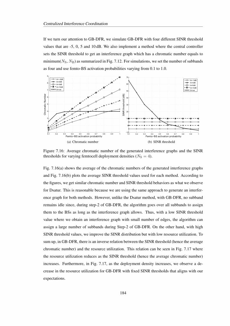
Centralized Interference Coordination
If we turn our attention to GB-DFR, we simulate GB-DFR with four different SINR threshold
values that are -5, 0, 5 and 10 dB. We also implement a method where the central controller
sets the SINR threshold to get an interference graph which has a chromatic number equals to
minimum(NS,NB) as summarized in Fig. 7.12. For simulations, we set the number of subbands
as four and use femto-BS activation probabilities varying from 0.1 to 1.0.
0.1 0.2 0.3 0.4 0.5 0.6 0.7 0.8 0.9 11
2
3
4
5
6
7
8
9
Femto−BSNactivationNprobability
Ch
rom
atic
NNu
mb
er
th=−5dB
th=0dB
th=5dB
th=10dB
th=var
(a) Chromatic number
0.1 0.2 0.3 0.4 0.5 0.6 0.7 0.8 0.9 1−10
0
10
20
30
40
50
60
70
Femto−BSRactivationRprobability
SIN
RRt
hre
sho
ldR[
dB
]
th=−5dB
th=0dB
th=5dB
th=10dB
th=var
(b) SINR threshold
Figure 7.16: Average chromatic number of the generated interference graphs and the SINRthresholds for varying femtocell deployment densities (NS = 4).
Fig. 7.16(a) shows the average of the chromatic numbers of the generated interference graphs
and Fig. 7.16(b) plots the average SINR threshold values used for each method. According to
the figures, we get similar chromatic number and SINR threshold behaviors as what we observe
for Dsatur. This is reasonable because we are using the same approach to generate an interfer-
ence graph for both methods. However, unlike the Dsatur method, with GB-DFR, no subband
remains idle since, during step-2 of GB-DFR, the algorithm goes over all subbands to assign
them to the BSs as long as the interference graph allows. Thus, with a low SINR threshold
value where we obtain an interference graph with small number of edges, the algorithm can
assign a large number of subbands during Step-2 of GB-DFR. On the other hand, with high
SINR threshold values, we improve the SINR distribution but with low resource utilization. To
sum up, in GB-DFR, there is an inverse relation between the SINR threshold (hence the average
chromatic number) and the resource utilization. This relation can be seen in Fig. 7.17 where
the resource utilization reduces as the SINR threshold (hence the average chromatic number)
increases. Furthermore, in Fig. 7.17, as the deployment density increases, we observe a de-
crease in the resource utilization for GB-DFR with fixed SINR thresholds that aligns with our
expectations.
184

Centralized Interference Coordination
0.1 0.2 0.3 0.4 0.5 0.6 0.7 0.8 0.9 120
30
40
50
60
70
80
90
100
Femto−BSuactivationuprobability
Res
ou
rceu
Uti
lizat
ion
uPer
cen
tag
e
th=−5dB
th=0dB
th=5dB
th=10dB
th=var
Figure 7.17: Resource utilization with respect to varying femtocell deployment densities (NS =4).
Figs. 7.18(a) and 7.18(b) show the average user capacities obtained with GB-DFR having dif-
ferent SINR thresholds for activation probability varies between 0.1 and 0.5 and between 0.5
and 1.0, respectively. Additionally, we compare their performance against the variable SINR
threshold implementation. In case the chromatic number of a constructed interference graph is
less than the total number of subbands, during the first step of GB-DFR, only NC subbands are
assigned. The rest subbands are assigned during the second step of GB-DFR. Thus, in such sit-
uations, if we increase the SINR threshold, we decrease the number of subbands to be assigned
during Step-2 due to the increase of edges in the graph. Therefore, unlike the Dsatur method,
for deployments where NC < NS, increasing the SINR threshold does not always provide
improved capacity performance. For instance, according to Fig. 7.18(a), for activation prob-
ability 0.3, by setting an SINR threshold to get a chromatic number equals to minimum(NS,
NB), the average cell capacity becomes lower than other GB-DFR methods having fixed SINR
thresholds. On the other hand, decreasing the SINR threshold, after some point, converges the
algorithm to reuse-1 with low SINR and capacity performance. For instance, GB-DFR with
-5 dB SINR threshold has worse average user capacity than 10 dB when femtocells are not
densely deployed, i.e. when the activation probability is 0.1 or 0.2.
If the chromatic number of a constructed interference graph happens to be larger than the num-
ber of subbands, NC > NS, the number of subbands becomes insufficient to solve all con-
flicts in the graph. By decreasing the SINR threshold until we get an interference graph with
NC = NS or even with NC < NS, we can manage to assign subbands to BSs without causing
any conflict during Step-1 of GB-DFR. Furthermore, more subbands can be assigned during
Step-2 that would lead to high resource utilization. Thus, we expect better performance when
185
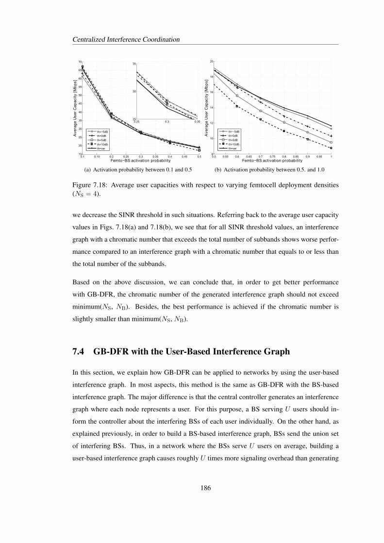
Centralized Interference Coordination
0.1 0.15 0.2 0.25 0.3 0.35 0.4 0.45 0.515
20
25
30
35
40
45
50
55
60
65
70
Femto−BSCactivationCprobability
Ave
rag
eCU
serC
Cap
acit
yC[M
bp
s]
th=−5dB
th=0dB
th=5dB
th=10dB
th=var
0.25 0.3 0.3525
30
35
(a) Activation probability between 0.1 and 0.5
0.5 0.55 0.6 0.65 0.7 0.75 0.8 0.85 0.9 0.95 18
10
12
14
16
18
20
Femto−BSsactivationsprobability
Ave
rag
esU
sers
Cap
acit
ys[M
bp
s]
th=−5dB
th=0dB
th=5dB
th=10dB
th=var
(b) Activation probability between 0.5. and 1.0
Figure 7.18: Average user capacities with respect to varying femtocell deployment densities(NS = 4).
we decrease the SINR threshold in such situations. Referring back to the average user capacity
values in Figs. 7.18(a) and 7.18(b), we see that for all SINR threshold values, an interference
graph with a chromatic number that exceeds the total number of subbands shows worse perfor-
mance compared to an interference graph with a chromatic number that equals to or less than
the total number of the subbands.
Based on the above discussion, we can conclude that, in order to get better performance
with GB-DFR, the chromatic number of the generated interference graph should not exceed
minimum(NS, NB). Besides, the best performance is achieved if the chromatic number is
slightly smaller than minimum(NS, NB).
7.4 GB-DFR with the User-Based Interference Graph
In this section, we explain how GB-DFR can be applied to networks by using the user-based
interference graph. In most aspects, this method is the same as GB-DFR with the BS-based
interference graph. The major difference is that the central controller generates an interference
graph where each node represents a user. For this purpose, a BS serving U users should in-
form the controller about the interfering BSs of each user individually. On the other hand, as
explained previously, in order to build a BS-based interference graph, BSs send the union set
of interfering BSs. Thus, in a network where the BSs serve U users on average, building a
user-based interference graph causes roughly U times more signaling overhead than generating
186
Centralized Interference Coordination
a BS-based interference graph.
In the user-based interference graph, a user u is connected to the users that are served by the
interfering BS of user u. As the central controller makes the resource assignment directly to
the users, instead of subbands, resource blocks are allocated to the users. Also, the users served
by the same cell should not be allocated the same resource blocks in order to prevent intra-
cell interference. Therefore, the users in the same cell are also connected in the constructed
interference graph.
The same modified graph coloring algorithm is applied to the user-based interference graph,
but, instead of the minimum subband criteria, we use the minimum number of resource blocks
that can be allocated to each user. Additionally, compared to the BS-based interference graph,
in the user-based interference graph, we have more nodes (as normally there are more users than
BSs) and more resources (as we use resource blocks instead of subbands). Therefore, the time
complexity at the controller to assign resources increases. On the other hand, as mentioned pre-
viously, applying GB-DFR with a large amount resources gives the controller more flexibility
to assign resources. Thus, compared to GB-DFR with the BS-based interference graph, higher
resource utilization is achieved with GB-DFR with the user-based interference graph.
After resource blocks are assigned to the users, the next step is to feed the corresponding as-
signment choices back to the BSs. It is clear that the central controller should indicate which
resource is assigned to which user separately. However, in the BS-based interference graph, the
central controller assigns subbands to BSs, so it only sends one resource indicator per BS. Thus,
for a network where BSs serve U users, informing the corresponding resource assignment to
the BSs requires approximately U times more signaling overhead in the user-based interference
graph method.
Fig. 7.19 shows the corresponding user-based interference graph that is generated by the central
controller. We use the same network deployment given in Fig. 7.4 that we use for illustrating
the GB-DFR with the BS-based interference graph. As can be seen in the figure, the difference
from Fig. 7.4 is that each BS sends feedback to the controller with the identities of their users
and the corresponding interfering BSs. Moreover, the interference graph at the controller shows
the relation between the users.
It is clear that as long as BSs in a network serve only one user, the generated user-based and
BS-based interference graphs are identical. However, as the number of users per cell increases,
187
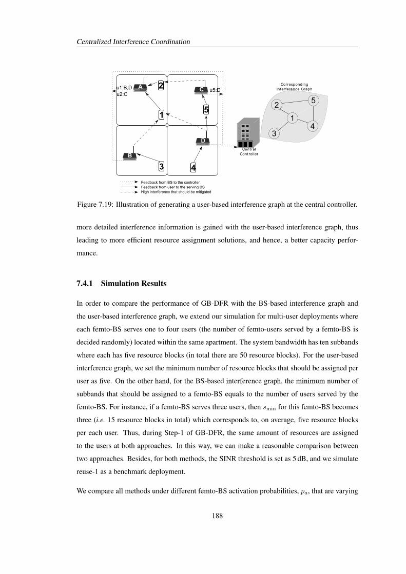
Centralized Interference Coordination
CentralDCont roller
CorrespondingDInterferenceDGraph
FeedbackDfromDBSDtoDtheDcontrollerFeedbackDfromDuserDtoDtheDservingDBSHighDinterferenceDthatDshouldDbeDmitigated
2
1
3
5
4
A
B
D
Cu1:B,D u5:Du2:C
3
2
14
5
Figure 7.19: Illustration of generating a user-based interference graph at the central controller.
more detailed interference information is gained with the user-based interference graph, thus
leading to more efficient resource assignment solutions, and hence, a better capacity perfor-
mance.
7.4.1 Simulation Results
In order to compare the performance of GB-DFR with the BS-based interference graph and
the user-based interference graph, we extend our simulation for multi-user deployments where
each femto-BS serves one to four users (the number of femto-users served by a femto-BS is
decided randomly) located within the same apartment. The system bandwidth has ten subbands
where each has five resource blocks (in total there are 50 resource blocks). For the user-based
interference graph, we set the minimum number of resource blocks that should be assigned per
user as five. On the other hand, for the BS-based interference graph, the minimum number of
subbands that should be assigned to a femto-BS equals to the number of users served by the
femto-BS. For instance, if a femto-BS serves three users, then smin for this femto-BS becomes
three (i.e. 15 resource blocks in total) which corresponds to, on average, five resource blocks
per each user. Thus, during Step-1 of GB-DFR, the same amount of resources are assigned
to the users at both approaches. In this way, we can make a reasonable comparison between
two approaches. Besides, for both methods, the SINR threshold is set as 5 dB, and we simulate
reuse-1 as a benchmark deployment.
We compare all methods under different femto-BS activation probabilities, pa, that are varying
188
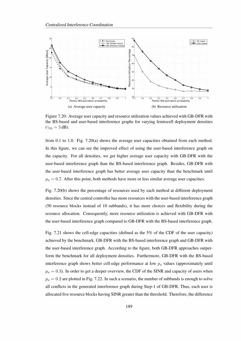
Centralized Interference Coordination
0.1 0.2 0.3 0.4 0.5 0.6 0.7 0.8 0.9 10
5
10
15
20
25
30
Femto−BSUactivationUprobability
Ave
rag
eUU
serU
Cap
acit
yU[M
bp
s]
BenchmarkGB−DFRGBS−basedDGB−DFRGUser−basedD
(a) Average user capacity
0.1 0.2 0.3 0.4 0.5 0.6 0.7 0.8 0.9 120
30
40
50
60
70
80
90
Femto−BSuactivationuprobability
Res
ou
rceu
Uti
lizat
ion
uPer
cen
tag
e
BS−basedUser−based
(b) Resource utilization
Figure 7.20: Average user capacity and resource utilization values achieved with GB-DFR withthe BS-based and user-based interference graphs for varying femtocell deployment densities(γth = 5 dB).
from 0.1 to 1.0. Fig. 7.20(a) shows the average user capacities obtained from each method.
In this figure, we can see the improved effect of using the user-based interference graph on
the capacity. For all densities, we get higher average user capacity with GB-DFR with the
user-based interference graph than the BS-based interference graph. Besides, GB-DFR with
the user-based interference graph has better average user capacity than the benchmark until
pa = 0.7. After this point, both methods have more or less similar average user capacities.
Fig. 7.20(b) shows the percentage of resources used by each method at different deployment
densities. Since the central controller has more resources with the user-based interference graph
(50 resource blocks instead of 10 subbands), it has more choices and flexibility during the
resource allocation. Consequently, more resource utilization is achieved with GB-DFR with
the user-based interference graph compared to GB-DFR with the BS-based interference graph.
Fig. 7.21 shows the cell-edge capacities (defined as the 5% of the CDF of the user capacity)
achieved by the benchmark, GB-DFR with the BS-based interference graph and GB-DFR with
the user-based interference graph. According to the figure, both GB-DFR approaches outper-
form the benchmark for all deployment densities. Furthermore, GB-DFR with the BS-based
interference graph shows better cell-edge performance at low pa values (approximately until
pa = 0.3). In order to get a deeper overview, the CDF of the SINR and capacity of users when
pa = 0.2 are plotted in Fig. 7.22. In such a scenario, the number of subbands is enough to solve
all conflicts in the generated interference graph during Step-1 of GB-DFR. Thus, each user is
allocated five resource blocks having SINR greater than the threshold. Therefore, the difference
189

Centralized Interference Coordination
0.1 0.2 0.3 0.4 0.5 0.6 0.7 0.8 0.9 10
0.5
1
1.5
2
2.5
3
3.5
4
4.5
5
Femto−BSdactivationdprobability
Cel
ldEd
ged
Cap
acit
yd[M
bp
s]
BenchmarkGB−DFRGBS−basedDGB−DFRGUser−basedD
Figure 7.21: Cell-edge user capacities achieved with varying femtocell deployment densities(γth = 5 dB).
between GB-DFR with the BS-based interference graph and with the user-based interference
graph mainly comes from the resource assignment during Step-2 of GB-DFR. As mentioned
previously, Step-2 of GB-DFR aims for increasing the resource utilization. Thus, with GB-DFR
with the user-based interference graph, cell-edge users are allocated less resources than other
users because they are connected to a large number of users in the graph. On the other hand,
with the BS-based interference graph, the BS which is assigned an extra subband during Step-2
(that corresponds to 1/10th of the bandwidth) can allocate this additional subband to its all users
including the cell-edge ones. Therefore, when the size of the interference graph small, there is
a high possibility that a BS gets an additional subband and allocates it to its cell-edge users.
On the other hand, as the deployment density increases, we can see the superiority of GB-DFR
−20 −10 0 10 20 30 40 50 600
0.1
0.2
0.3
0.4
0.5
0.6
0.7
0.8
0.9
1
SINRG[dB]
CD
F
Benchmark
GB−DFR(BS−based)
GB−DFR(User−based)
(a) CDF of the SINR
0 10 20 30 40 50 600
0.1
0.2
0.3
0.4
0.5
0.6
0.7
0.8
0.9
1
UserhCapacityh[Mbps]
CD
F
Benchmark
GB−DFR)BS−based)
GB−DFR)User−based)
(b) CDF of the capacity
Figure 7.22: SINR and capacity performance of GB-DFR with the user and BS-based interfer-ence graphs (pa = 0.2, γth = 5 dB).
190
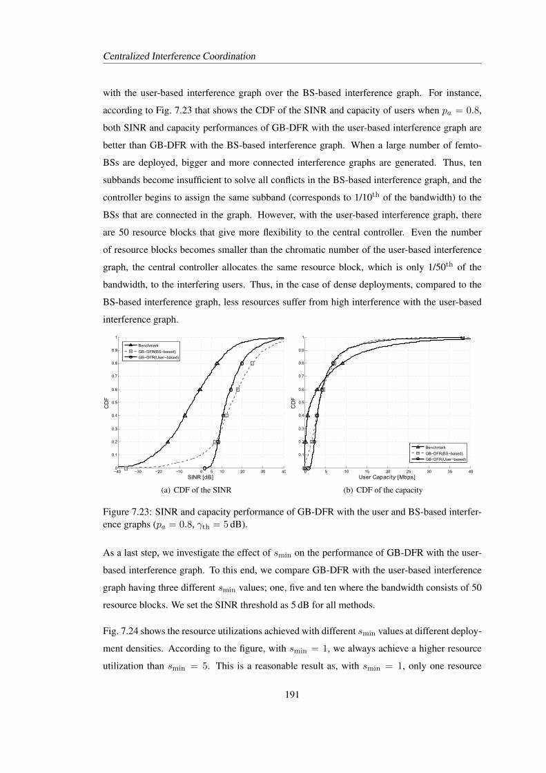
Centralized Interference Coordination
with the user-based interference graph over the BS-based interference graph. For instance,
according to Fig. 7.23 that shows the CDF of the SINR and capacity of users when pa = 0.8,
both SINR and capacity performances of GB-DFR with the user-based interference graph are
better than GB-DFR with the BS-based interference graph. When a large number of femto-
BSs are deployed, bigger and more connected interference graphs are generated. Thus, ten
subbands become insufficient to solve all conflicts in the BS-based interference graph, and the
controller begins to assign the same subband (corresponds to 1/10th of the bandwidth) to the
BSs that are connected in the graph. However, with the user-based interference graph, there
are 50 resource blocks that give more flexibility to the central controller. Even the number
of resource blocks becomes smaller than the chromatic number of the user-based interference
graph, the central controller allocates the same resource block, which is only 1/50th of the
bandwidth, to the interfering users. Thus, in the case of dense deployments, compared to the
BS-based interference graph, less resources suffer from high interference with the user-based
interference graph.
−40 −30 −20 −10 0 5 10 20 30 400
0.1
0.2
0.3
0.4
0.5
0.6
0.7
0.8
0.9
1
SINRG[dB]
CD
F
Benchmark
GB−DFR(BS−based)
GB−DFR(User−based)
(a) CDF of the SINR
0 5 10 15 20 25 30 35 400
0.1
0.2
0.3
0.4
0.5
0.6
0.7
0.8
0.9
1
UserhCapacityh[Mbps]
CD
F
Benchmark
GB−DFR)BS−based)
GB−DFR)User−based)
(b) CDF of the capacity
Figure 7.23: SINR and capacity performance of GB-DFR with the user and BS-based interfer-ence graphs (pa = 0.8, γth = 5 dB).
As a last step, we investigate the effect of smin on the performance of GB-DFR with the user-
based interference graph. To this end, we compare GB-DFR with the user-based interference
graph having three different smin values; one, five and ten where the bandwidth consists of 50
resource blocks. We set the SINR threshold as 5 dB for all methods.
Fig. 7.24 shows the resource utilizations achieved with different smin values at different deploy-
ment densities. According to the figure, with smin = 1, we always achieve a higher resource
utilization than smin = 5. This is a reasonable result as, with smin = 1, only one resource
191
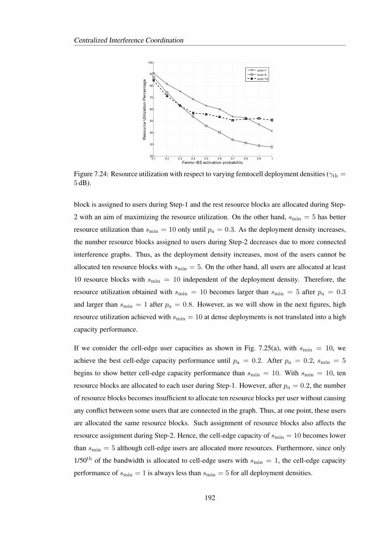
Centralized Interference Coordination
0.1 0.2 0.3 0.4 0.5 0.6 0.7 0.8 0.9 120
30
40
50
60
70
80
90
100
Femto−BSuactivationuprobability
Res
ou
rceu
Uti
lizat
ion
uPer
cen
tag
e
smin=1
smin=5
smin=10
Figure 7.24: Resource utilization with respect to varying femtocell deployment densities (γth =5 dB).
block is assigned to users during Step-1 and the rest resource blocks are allocated during Step-
2 with an aim of maximizing the resource utilization. On the other hand, smin = 5 has better
resource utilization than smin = 10 only until pa = 0.3. As the deployment density increases,
the number resource blocks assigned to users during Step-2 decreases due to more connected
interference graphs. Thus, as the deployment density increases, most of the users cannot be
allocated ten resource blocks with smin = 5. On the other hand, all users are allocated at least
10 resource blocks with smin = 10 independent of the deployment density. Therefore, the
resource utilization obtained with smin = 10 becomes larger than smin = 5 after pa = 0.3
and larger than smin = 1 after pa = 0.8. However, as we will show in the next figures, high
resource utilization achieved with smin = 10 at dense deployments is not translated into a high
capacity performance.
If we consider the cell-edge user capacities as shown in Fig. 7.25(a), with smin = 10, we
achieve the best cell-edge capacity performance until pa = 0.2. After pa = 0.2, smin = 5
begins to show better cell-edge capacity performance than smin = 10. With smin = 10, ten
resource blocks are allocated to each user during Step-1. However, after pa = 0.2, the number
of resource blocks becomes insufficient to allocate ten resource blocks per user without causing
any conflict between some users that are connected in the graph. Thus, at one point, these users
are allocated the same resource blocks. Such assignment of resource blocks also affects the
resource assignment during Step-2. Hence, the cell-edge capacity of smin = 10 becomes lower
than smin = 5 although cell-edge users are allocated more resources. Furthermore, since only
1/50th of the bandwidth is allocated to cell-edge users with smin = 1, the cell-edge capacity
performance of smin = 1 is always less than smin = 5 for all deployment densities.
192
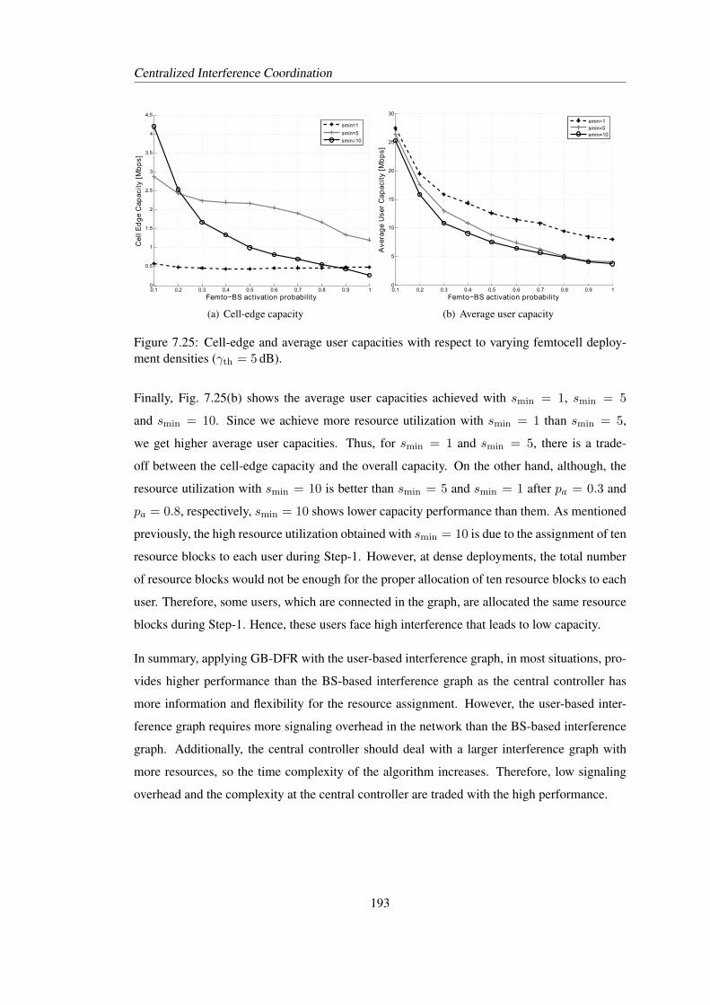
Centralized Interference Coordination
0.1 0.2 0.3 0.4 0.5 0.6 0.7 0.8 0.9 10
0.5
1
1.5
2
2.5
3
3.5
4
4.5
Femto−BSdactivationdprobability
Cel
ldEd
ged
Cap
acit
yd[M
bp
s]
smin=1
smin=5
smin=10
(a) Cell-edge capacity
0.1 0.2 0.3 0.4 0.5 0.6 0.7 0.8 0.9 10
5
10
15
20
25
30
Femto−BSUactivationUprobability
Ave
rag
eUU
serU
Cap
acit
yU[M
bp
s]
smin=1smin=5smin=10
(b) Average user capacity
Figure 7.25: Cell-edge and average user capacities with respect to varying femtocell deploy-ment densities (γth = 5 dB).
Finally, Fig. 7.25(b) shows the average user capacities achieved with smin = 1, smin = 5
and smin = 10. Since we achieve more resource utilization with smin = 1 than smin = 5,
we get higher average user capacities. Thus, for smin = 1 and smin = 5, there is a trade-
off between the cell-edge capacity and the overall capacity. On the other hand, although, the
resource utilization with smin = 10 is better than smin = 5 and smin = 1 after pa = 0.3 and
pa = 0.8, respectively, smin = 10 shows lower capacity performance than them. As mentioned
previously, the high resource utilization obtained with smin = 10 is due to the assignment of ten
resource blocks to each user during Step-1. However, at dense deployments, the total number
of resource blocks would not be enough for the proper allocation of ten resource blocks to each
user. Therefore, some users, which are connected in the graph, are allocated the same resource
blocks during Step-1. Hence, these users face high interference that leads to low capacity.
In summary, applying GB-DFR with the user-based interference graph, in most situations, pro-
vides higher performance than the BS-based interference graph as the central controller has
more information and flexibility for the resource assignment. However, the user-based inter-
ference graph requires more signaling overhead in the network than the BS-based interference
graph. Additionally, the central controller should deal with a larger interference graph with
more resources, so the time complexity of the algorithm increases. Therefore, low signaling
overhead and the complexity at the central controller are traded with the high performance.
193
Centralized Interference Coordination
7.5 Extended Graph-Based Dynamic Frequency Reuse
Up to now, we proposed two interference avoidance approaches based on the frequency parti-
tioning between cells; in the distributed algorithms mentioned in Chapter 5 and 6, BSs assign
their own resources autonomously, whereas, in GB-DFR, a central controller is responsible
for the resource assignment. As we mention, both approaches have their own advantages and
drawbacks. In the distributed algorithms, we have low complexity as each BS optimizes the
resource assignment according to local information, and the complexity of the algorithm does
not depend on the size of the network. On the other hand, in GB-DFR, the complexity at
the controller increases as the number of deployed BSs increases. Nevertheless, we reach a
stable resource assignment shortly with GB-DFR. As we mentioned in the previous section,
the performance of GB-DFR with the BS-based interference graph decreases as BSs start to
serve multiple users. The performance can be improved with GB-DFR with the user-based
interference graph, but this would cost high complexity at the central controller. Therefore,
in this section, by taking the strong sides of the distributed and central resource assignment
approaches, we propose eGB-DFR that is better suited to serve multi-user scenarios with the
objective of increasing the cell-edge capacity whilst maintaining a high subband utilization. For
this purpose, we define two classes of subbands depending on their foreseen usage by a BS: the
primary-subband, which is assigned by a central controller and the secondary-subband which
is assigned by BSs autonomously. This is, therefore, a hybrid method comprising a centralized
and a decentralized component.
Primary-subbands are the subbands that are reserved for protection of cell-edge users facing
high interference. If a particular subband is used by a BS as a primary-subband, then neigh-
boring BSs which have the potential to cause interference to the cell in question are forbidden
from using the same subband. A BS intending to use a particular subband as a primary-subband
needs to inform its interfering neighbors so that the interfering neighbors do not use this sub-
band. This is done via the transmission of a so-called primary-subband indicator between
BSs. When a BS receives such a message, it does not transmit any data over the marked sub-
band, thereby reducing the interference caused to its neighboring cells. Thus, the usage of the
primary-subbands augments the cell-edge capacity.
The subbands which remain unmarked, i.e., non-primary subbands, may be used by a BS as a
secondary-subband depending on the prevailing interference conditions, but enjoying no priv-
ileges, these subbands cannot be blocked at interfering neighboring BSs. Secondary-subbands
194

Centralized Interference Coordination
can, therefore, be allocated to cell-center users that face low interference as long as these sub-
bands do not cause high interference to neighboring BSs. In this way, the spatial reuse of
resources increases especially for cell-center users.
Since cell-edge users have low SINR because of high interference, they operate in the power-
limited region. For these users, increasing SINR leads to more capacity improvement than
increasing the bandwidth. Thus, these users can give up some bandwidth in return for im-
proved capacity. On the other hand, cell-center users have high SINR and mostly operate in the
bandwidth-limited region. For these users, increasing the SINR does not provide a significant
improvement in capacity. Therefore, decreasing resources of these users for further enhance-
ment of their SINR levels causes capacity degradation. This is why, in DASA, we assign pro-
tected primary-subbands to cell-edge users to improve their SINRs and hence their capacities.
Additionally, by assigning secondary-subbands to cell-center users, we do not cause remark-
able decrease in the resource utilization of these users and hence they do not face unacceptable
capacity loss.
To clarify the aim of DASA, a toy example of the assignment of subbands by BSs is depicted in
Fig. 7.26. According to Fig. 7.26, femto-BSs serve users that are located in the same apartment;
fBS1 serves two users and fBS2 and fBS3 serve one user. Each femto-BS has three subbands,
S1, S2 and S3, available to it. The arrows indicate strong interference that should be mitigated
to achieve the desired service quality which is the target SINR threshold. In the example de-
ployment, user-1 suffers from severe interference from fBS2 and fBS3, and resources allocated
to it should not face any interference from these femto-BSs. In a similar manner, resources
allocated to user-3 should be protected from fBS1 and fBS3.
As can be seen in the figure, fBS1 uses S1 as a primary-subband for protection of its cell-edge
user that is user-1. Therefore, the use of S1 by fBS2 and fBS3, which cause high interference
to user-1, should be blocked. Similarly, fBS1 and fBS3 should not transmit data over S2 which
is used by fBS2 as a primary-subband to protect user-3. Other users in the network do not
need any proactive protection to achieve the target service quality. Therefore, S3, which is the
primary-subband of fBS3, is not needed to be blocked at fBS1 and fBS2. Subband S3 that
is not blocked at fBS1 and fBS2 might be used as a secondary-subband at these femto-BSs.
According to the figure, fBS1 can allocate the resources of S3 to user-2 since it does not face
severe interference from fBS2 and fBS3. On the other hand, fBS2 cannot use S3 as a secondary-
subband despite not being blocked since user-3 receives strong interference over S3. Thus, we
195
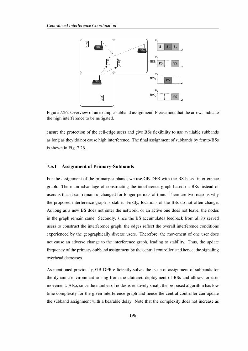
Centralized Interference Coordination
U1
U4
fBS1
fBS3
U3
fBS2
U2 S1 S2 S3
p
f
PS SS
p
f
fBS1
PS
p
f
fBS2
PS
p
fPS
p
f
fBS3
Figure 7.26: Overview of an example subband assignment. Please note that the arrows indicatethe high interference to be mitigated.
ensure the protection of the cell-edge users and give BSs flexibility to use available subbands
as long as they do not cause high interference. The final assignment of subbands by femto-BSs
is shown in Fig. 7.26.
7.5.1 Assignment of Primary-Subbands
For the assignment of the primary-subband, we use GB-DFR with the BS-based interference
graph. The main advantage of constructing the interference graph based on BSs instead of
users is that it can remain unchanged for longer periods of time. There are two reasons why
the proposed interference graph is stable. Firstly, locations of the BSs do not often change.
As long as a new BS does not enter the network, or an active one does not leave, the nodes
in the graph remain same. Secondly, since the BS accumulates feedback from all its served
users to construct the interference graph, the edges reflect the overall interference conditions
experienced by the geographically diverse users. Therefore, the movement of one user does
not cause an adverse change to the interference graph, leading to stability. Thus, the update
frequency of the primary-subband assignment by the central controller, and hence, the signaling
overhead decreases.
As mentioned previously, GB-DFR efficiently solves the issue of assignment of subbands for
the dynamic environment arising from the cluttered deployment of BSs and allows for user
movement. Also, since the number of nodes is relatively small, the proposed algorithm has low
time complexity for the given interference graph and hence the central controller can update
the subband assignment with a bearable delay. Note that the complexity does not increase as
196
Centralized Interference Coordination
the number of served users increases. Additionally, the rate of change of the interference graph
is low which reduces the need for the central controller to update the subband assignment fre-
quently. Consequently, applying GB-DFR with the BS-based interference graph by a central
controller is a convenient approach for assigning the primary-subbands to BSs. It is guaran-
teed that the interfering BSs use different primary-subbands as long as the interference graph
remains unchanged. However, the interference graph cannot reflect all interference information
especially when users in the same cell face different interference conditions. For example, as-
sume BS b is assigned multiple subbands, say subbands 1 and 2, after applying GB-DFR. Since
all neighbors of BS b in the interference graph are forbidden from using these subbands, the
cell-edge users of BS b are protected. However, for the cell-center users that do not need protec-
tion, BS b does not need to restrict its neighbors. Thus, if BS b uses subband 1 for the cell-edge
users and subband 2 for the cell-center users, then the neighbors of BS b are not blocked from
using subband 2. In this way, more subbands can be utilized. This gives an indication as to
why we need to classify subbands as primary-subbands and secondary-subbands. For this pur-
pose in eGB-DFR, we apply only the first step of GB-DFR for assigning the primary-subbands
by setting smin as the number of the primary-subband per BS. The rest of the subbands are
assigned as a secondary-subband autonomously by BSs.
After the primary-subbands are assigned, the BS in question can inform the (potential) interfer-
ing BSs of its served users via a primary-subband indicator. By doing so, the serving BS blocks
the interfering BSs for using its primary-subband, and the desired SINR threshold, γth can be
achieved at the given users. The serving BS sends the primary-subband indicator only for those
users to which resource blocks from the primary-subband are allocated, i.e., cell-edge users.
7.5.2 Assignment of Secondary-Subbands
The secondary-subbands, belonging to the set of all unblocked (in other words, non-primary-
subbands) subbands are assigned autonomously by BSs after primary-subbands are assigned.
Similar to the primary-subband, the same SINR threshold is set for the secondary-subbands.
Thus, a BS can assign a subband as a secondary-subband if any of its served users experiences
an SINR higher than the predefined SINR threshold. Therefore, a BS can assign a subband as
a secondary-subband if both of the following conditions hold:
• The subband is not marked by any neighboring BS as a primary-subband, in other words,
197
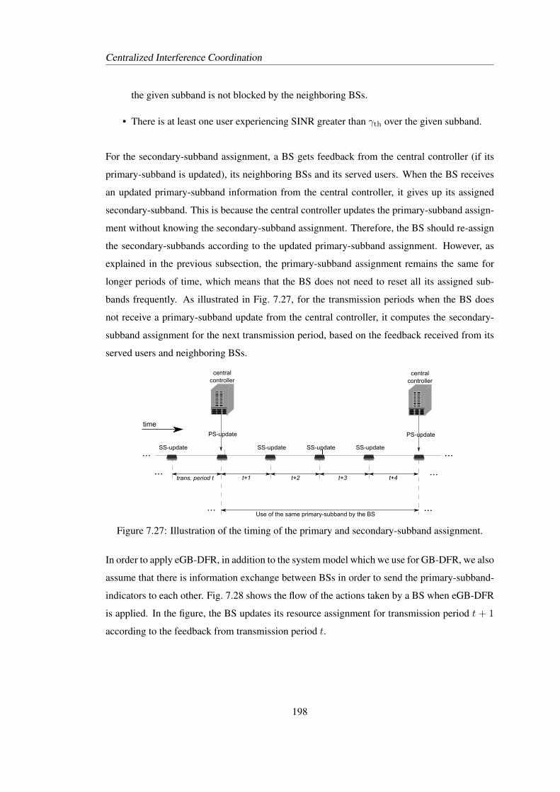
Centralized Interference Coordination
the given subband is not blocked by the neighboring BSs.
• There is at least one user experiencing SINR greater than γth over the given subband.
For the secondary-subband assignment, a BS gets feedback from the central controller (if its
primary-subband is updated), its neighboring BSs and its served users. When the BS receives
an updated primary-subband information from the central controller, it gives up its assigned
secondary-subband. This is because the central controller updates the primary-subband assign-
ment without knowing the secondary-subband assignment. Therefore, the BS should re-assign
the secondary-subbands according to the updated primary-subband assignment. However, as
explained in the previous subsection, the primary-subband assignment remains the same for
longer periods of time, which means that the BS does not need to reset all its assigned sub-
bands frequently. As illustrated in Fig. 7.27, for the transmission periods when the BS does
not receive a primary-subband update from the central controller, it computes the secondary-
subband assignment for the next transmission period, based on the feedback received from its
served users and neighboring BSs.
PS-update
SS-update
time
...
Use of the same primary-subband by the BS
central controller
PS-update
central controller
SS-update SS-updateSS-update...
trans. period t t+1 t+2 t+3 t+4... ...
... ...
Figure 7.27: Illustration of the timing of the primary and secondary-subband assignment.
In order to apply eGB-DFR, in addition to the system model which we use for GB-DFR, we also
assume that there is information exchange between BSs in order to send the primary-subband-
indicators to each other. Fig. 7.28 shows the flow of the actions taken by a BS when eGB-DFR
is applied. In the figure, the BS updates its resource assignment for transmission period t + 1
according to the feedback from transmission period t.
198
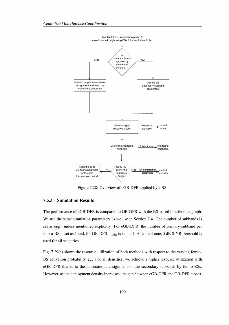
Centralized Interference Coordination
UpdateNtheNprimaryNsubbandassignmentNandNresetNthe
secondaryNsubbands
YES
feedbackNfromNtransmissionNperiodNtservedNusersNxNneighboringNBSsNxNtheNcentralNcontroller
IsNprimaryNsubband
NupdatedNbyNtheNcentralNcontroller?
DoesNtheNinterferingNneighborschange?
SchedulingNofNresourceNblocks
NO
ResourceNallocation
UpdateNtheNsecondaryNsubband
assignment
DefineNtheNinterferingneighbors
servedusers
interferingNneighbors
centralcontroller
PS-indicator
IDNofNinterferingneighbors
YESNOKeepNtheNIDNofN
interferingNneighborsNforNtheNnextN
transmissionNperiod
Figure 7.28: Overview of eGB-DFR applied by a BS.
7.5.3 Simulation Results
The performance of eGB-DFR is compared to GB-DFR with the BS-based interference graph.
We use the same simulation parameters as we use in Section 7.4. The number of subbands is
set as eight unless mentioned explicitly. For eGB-DFR, the number of primary-subband per
femto-BS is set as 1 and, for GB-DFR, smin is set as 1. As a final note, 5 dB SINR threshold is
used for all scenarios.
Fig. 7.29(a) shows the resource utilization of both methods with respect to the varying femto-
BS activation probability, pa. For all densities, we achieve a higher resource utilization with
eGB-DFR thanks to the autonomous assignment of the secondary-subbands by femto-BSs.
However, as the deployment density increases, the gap between eGB-DFR and GB-DFR closes.
199
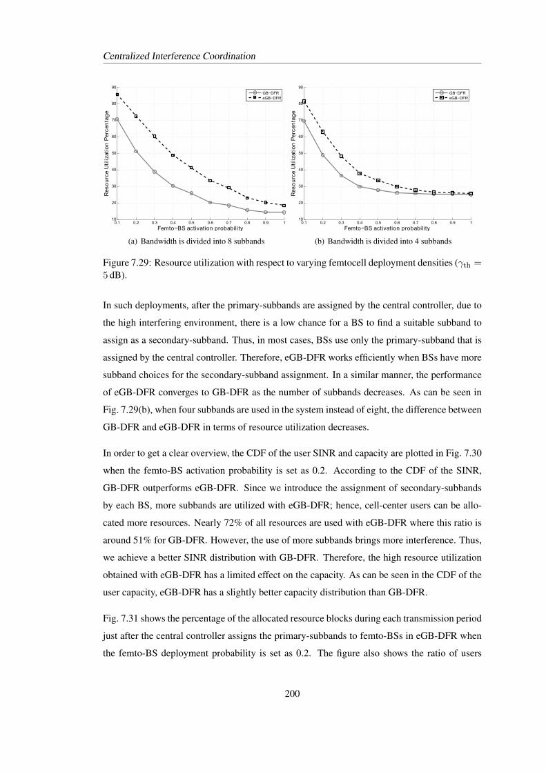
Centralized Interference Coordination
0.1 0.2 0.3 0.4 0.5 0.6 0.7 0.8 0.9 110
20
30
40
50
60
70
80
90
Femto−BSuactivationuprobability
Res
ou
rceu
Uti
lizat
ion
uPer
cen
tag
e
GB−DFReGB−DFR
(a) Bandwidth is divided into 8 subbands
0.1 0.2 0.3 0.4 0.5 0.6 0.7 0.8 0.9 110
20
30
40
50
60
70
80
90
Femto−BSuactivationuprobability
Res
ou
rceu
Uti
lizat
ion
uPer
cen
tag
e
GB−DFReGB−DFR
(b) Bandwidth is divided into 4 subbands
Figure 7.29: Resource utilization with respect to varying femtocell deployment densities (γth =5 dB).
In such deployments, after the primary-subbands are assigned by the central controller, due to
the high interfering environment, there is a low chance for a BS to find a suitable subband to
assign as a secondary-subband. Thus, in most cases, BSs use only the primary-subband that is
assigned by the central controller. Therefore, eGB-DFR works efficiently when BSs have more
subband choices for the secondary-subband assignment. In a similar manner, the performance
of eGB-DFR converges to GB-DFR as the number of subbands decreases. As can be seen in
Fig. 7.29(b), when four subbands are used in the system instead of eight, the difference between
GB-DFR and eGB-DFR in terms of resource utilization decreases.
In order to get a clear overview, the CDF of the user SINR and capacity are plotted in Fig. 7.30
when the femto-BS activation probability is set as 0.2. According to the CDF of the SINR,
GB-DFR outperforms eGB-DFR. Since we introduce the assignment of secondary-subbands
by each BS, more subbands are utilized with eGB-DFR; hence, cell-center users can be allo-
cated more resources. Nearly 72% of all resources are used with eGB-DFR where this ratio is
around 51% for GB-DFR. However, the use of more subbands brings more interference. Thus,
we achieve a better SINR distribution with GB-DFR. Therefore, the high resource utilization
obtained with eGB-DFR has a limited effect on the capacity. As can be seen in the CDF of the
user capacity, eGB-DFR has a slightly better capacity distribution than GB-DFR.
Fig. 7.31 shows the percentage of the allocated resource blocks during each transmission period
just after the central controller assigns the primary-subbands to femto-BSs in eGB-DFR when
the femto-BS deployment probability is set as 0.2. The figure also shows the ratio of users
200
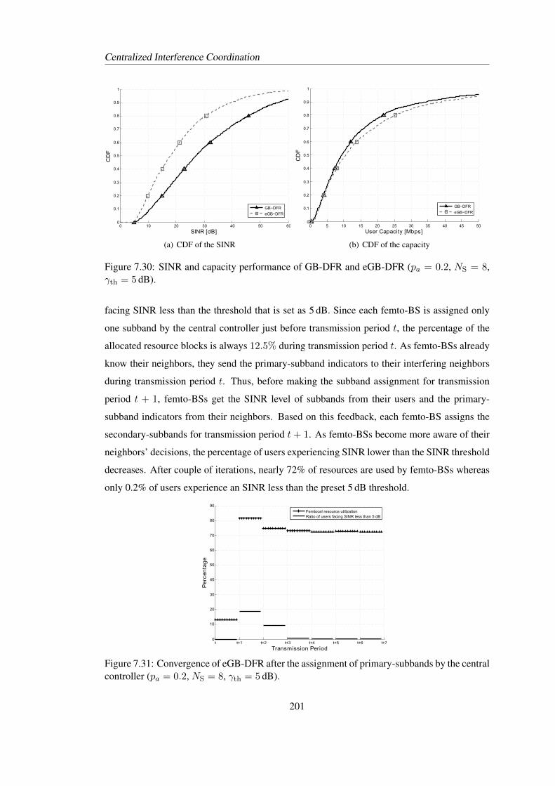
Centralized Interference Coordination
0 10 20 30 40 50 600
0.1
0.2
0.3
0.4
0.5
0.6
0.7
0.8
0.9
1
SINR [dB]
CD
F
GB−DFR
eGB−DFR
(a) CDF of the SINR
0 5 10 15 20 25 30 35 40 45 500
0.1
0.2
0.3
0.4
0.5
0.6
0.7
0.8
0.9
1
UserRCapacityR[Mbps]
CD
F
GB−DFR
eGB−DFR
(b) CDF of the capacity
Figure 7.30: SINR and capacity performance of GB-DFR and eGB-DFR (pa = 0.2, NS = 8,γth = 5 dB).
facing SINR less than the threshold that is set as 5 dB. Since each femto-BS is assigned only
one subband by the central controller just before transmission period t, the percentage of the
allocated resource blocks is always 12.5% during transmission period t. As femto-BSs already
know their neighbors, they send the primary-subband indicators to their interfering neighbors
during transmission period t. Thus, before making the subband assignment for transmission
period t + 1, femto-BSs get the SINR level of subbands from their users and the primary-
subband indicators from their neighbors. Based on this feedback, each femto-BS assigns the
secondary-subbands for transmission period t + 1. As femto-BSs become more aware of their
neighbors’ decisions, the percentage of users experiencing SINR lower than the SINR threshold
decreases. After couple of iterations, nearly 72% of resources are used by femto-BSs whereas
only 0.2% of users experience an SINR less than the preset 5 dB threshold.
t t+1 t+2 t+3 t+4 t+5 t+6 t+70
10
20
30
40
50
60
70
80
90
TransmissionfPeriod
Per
cen
tag
e
FemtocelfresourcefutilizationRatiofoffusersffacingfSINRflessfthanf5fdB
Figure 7.31: Convergence of eGB-DFR after the assignment of primary-subbands by the centralcontroller (pa = 0.2, NS = 8, γth = 5 dB).
201
Centralized Interference Coordination
To conclude, eGB-DFR does not offer a significant improvement compared to GB-DFR. How-
ever, it offers a different approach of graph coloring implementation. With eGB-DFR, the
complexity at the central controller decreases, however the method requires a signaling of the
primary-subband indicator between BSs. Thus, with eGB-DFR, complexity at the central con-
troller is traded-off with the signaling overhead between BSs.
7.6 Conclusion
In this chapter, we investigate the centrally-managed interference avoidance techniques in fem-
tocell networks. For this purpose, we use the graph coloring algorithms, where the central con-
troller carries out the resource assignment according to an interference graph. The proposed
GB-DFR can adaptively match the frequency reuse in unplanned wireless networks depending
on varying interference conditions. Unlike the conventional graph coloring, where the same
amount of resources is always allocated to the BSs, GB-DFR assigns more resources to the
BSs that are exposed to less severe interference conditions. Also, with the use of the minimum
subband per BS restriction, fairness, in terms of assigned resources, can be adapted among
BSs. As the method relies on the measurements of users, it is able to dynamically adapt to
the interference conditions faced in random deployments; thus balancing high spatial reuse of
subbands with interference protection for cell-edge users. In GB-DFR, it is also possible to
build the interference graph according to the users. GB-DFR with the user-based interference
graph lets us achieve an interference protection with high capacity performance. GB-DFR with
the BS-based interference graph, on the other hand, offers an interference avoidance with less
signaling complexity.
In addition to GB-DFR, we also propose the eGB-DFR method which takes the advantages of
both central and autonomous resource assignment approaches. In eGB-DFR, by assigning the
primary-subbands centrally, the system reaches a stable resource assignment in a short time,
and the cell-edge users are well-protected. Additionally, by assigning the secondary-subbands
autonomously, a BS gets more flexibility in choosing subbands available for transmission, so
the utilization of subbands increases. Although the complexity at the central controller de-
creases with eGB-DFR, BSs need to signal their primary-subband information to their inter-
fering neighbors. Simulation results indicate that eGB-DFR provides a slightly better capacity
performance than GB-DFR with the BS-based interference graph when cells are serving mul-
tiple users. However, as the deployment density of femto-BSs increases, both methods start to
202
Centralized Interference Coordination
show similar performances because BSs assign a small number of secondary-subbands due to
high interfering environment.
Furthermore, the signaling assumptions used for developing the proposed methods are mostly
standardized in LTE and LTE-A such as the received signal power measurement reports and
the SINR measurements. Besides, like DASA, we do not introduce any extra complexity at the
user side where only BSs and the central controller apply the proposed algorithms. As a final
remark, although we explain the proposed methods based on femtocell networks, they can be
applied to any uncoordinated network.
203

Centralized Interference Coordination
204
Chapter 8Conclusion
This thesis aims at handling downlink interference in small cell networks that can be applied
to commercial Long-Term Evolution (LTE) and Long-Term Evolution-Advanced (LTE-A) net-
works. Small cells are deployed over the macrocell layer, and we call these multi-layered
networks heterogeneous networks (Het-Nets). We mention in Chapter 2 that Het-Net deploy-
ments gain significant interest as they can provide a remarkable improvement on overall data
rates. Because of their small size and low cost compared to macro-base stations (BSs), intro-
duction of small cells would lead to a dense deployment of BSs. This eventually causes high
co-channel interference between cells, which constitutes the main topic of our work.
Small cells are differentiated according to their use area, where the well-known small cells
are picocells, microcells and femtocells. Each small cell type requires distinct implementation
specifications; thus, each of them has its own interference scenario. We generate interference
handling methods by taking femtocell networks as a system model. In such networks, end users
can deploy their own BSs in their premises and can change their locations or switch them off
anytime. As the position and the status of these BSs can vary, the operator cannot have an
efficient frequency planning and optimization for these networks. Consequently, interference
management in femtocell networks is more challenging than in other small cell deployments,
and we need novel techniques that are specific to this type of networks having dynamic interfer-
ence environment. To this end, we give a detailed overview of femtocell networks in Chapter 3,
which helps to understand their system architecture and operation policies. The simulation
results indicate that interference between femtocells becomes significant as the deployment
205
Conclusion
density of BSs increases. Additionally, the level of interference directly depends on the access
policies of femto-BSs. Open-access femto-BSs are like macro-BSs, and they can serve users in
a network without any restriction. However, closed access femto-BSs provide service only to
the subscribed users. Therefore, such kind of deployments causes more interference to femto
and macro-users.
After defining the source of interference, as a next step, we decide on interference handling
approaches that we can apply effectively to femtocell networks. Thus, in Chapter 4, we discuss
different approaches varying from theoretical methods to practical techniques. The interfer-
ence handling method that is suited for femtocell networks should be dynamic in a sense that
it can update itself according to changes in the environment. Furthermore, femto-BSs are not
as advanced as macro-BSs because they are purchased by end users for an indoor usage. Ad-
ditionally, the backhaul limitation should be considered for such networks as these devices are
connected to the core network, mostly, via the digital subscriber line (DSL) service. Although,
the theoretical methods provide solutions with a remarkable performance, they are not appropri-
ate for real networks, so we direct our attention to interference management techniques that are
provided by LTE and LTE-A networks. Among the techniques we present in Chapter 4; inter-
ference avoidance by resource partitioning is found to be the most promising candidate as it can
be applied to femtocell networks with the least complexity. Moreover, via inter-cell interfer-
ence coordination (ICIC) and enhanced inter-cell interference coordination (eICIC) techniques,
LTE and LTE-A already support the signaling between BSs that is required for the coordination
of BSs.
In Chapter 5, we investigate the effect of interference on the control channel transmission in
LTE and LTE-A systems. The protection of the control channels is crucial for reliable data
transmissions; otherwise, received data cannot be decoded by users. After investigating the
physical layer of LTE and LTE-A, we develop techniques that are based on time-domain and
frequency-domain protections. For this purpose, we use techniques already defined in the stan-
dards; almost blank subframes (ABSs) and cross-carrier scheduling. Both techniques are serv-
ing for the protection of the control channels between cells. However, these methods are devel-
oped for removing interference between different layers in Het-Net deployments, i.e., interfer-
ence between a macrocell and a femtocell or between a macrocell and a picocell. Thus, they do
not offer any dynamic protection, especially between small cells. The techniques introduced
in this chapter address this problem and provide a remarkable performance to protect the users
206
Conclusion
from going into an outage.
In order to protect the cell-edge users from the detrimental effect of interference, we develop
several methods based on the resource partitioning. Our goal is to build a method that protects
the cell-edge users according to the varying interference conditions and achieves high resource
utilization. Based on the stated targets, in Chapter 6, we introduce dynamic and autonomous
subband assignment (DASA) where BSs assign the resources in a distributed way. In Chapter 7,
we build graph-based dynamic frequency reuse (GB-DFR) for centrally controlled networks
where the central controller is responsible for the assignment of resources. Furthermore, we
propose a hybrid method, extended graph-based dynamic frequency reuse (eGB-DFR), that is
based on the central and distributed approaches. For all proposed methods, we assume fem-
tocell networks with an LTE air interface as a basis. However, it is possible to apply these
methods to any uncoordinated dynamic networks with minor changes.
In this thesis, we develop methods by assuming full-buffer traffic that is the worst-case sce-
nario. As a future work, adapting the methods to networks with varying traffic scenarios would
give us a deep insight for more realistic deployments. Additionally, we consider a static envi-
ronment where the locations of the users do not change. Therefore, testing the performance of
the developed methods with simulation scenarios with moving users is another point to be in-
vestigated. Nevertheless, indoor users do not have high speed. Thus, the impact of the mobility
on the proposed methods is expected to be negligible.
We develop methods for protecting the data and control region separately. Although the meth-
ods developed in Chapter 5 provide a data region protection to some extent, the combination of
these methods with the ones developed for the data region protection in Chapters 6 and 7 in the
same system is another open topic to be studied.
We only consider the downlink direction and the extension of the proposed methods for the
uplink direction would be a further research direction. Moreover, energy efficiency becomes
one of the prospective topics of the wireless industry. Since our methods are based on assigning
resources to BSs according to the interference environment, we can extend our work by consid-
ering the energy consumption issues. For instance, under low traffic loads, BSs give up some
of their resources in a coordinated way such that they reduce the energy consumption as well
as achieve a cell-edge protection.
207

Conclusion
208
Appendix AList of Publications
This section contains a list of published papers and the patents related with the thesis.
A.1 Papers
• S. Uygungelen, G. Auer, and Z. Bharucha, “Graph-Based Dynamic Frequency Reuse
in Femtocell Networks,” in Proc. of the 73rd IEEE Vehicular Technology Conference
(VTC), Budapest, Hungary, May 15–18 2011.
• S. Uygungelen, Z. Bharucha and G. Auer, “Interference Coordination via Autonomous
Component Carrier Assignment,” in Proc. of the 54th IEEE Global Telecommunications
Conference (GLOBECOM), Houston, USA, Dec. 5–9 2011.
• S. Uygungelen and Z. Bharucha, “A Dynamic Resource Assignment Method for Uncoor-
dinated Wireless Networks,” in Proc. of the 76th IEEE Vehicular Technology Conference
(VTC), Quebec City, Canada, Sep. 3–6 2012.
• S. Uygungelen, Z. Bharucha and H. Taoka, “Control Region Protection in LTE-A Net-
works,” in Proc. of the 23rd IEEE International Symposium on Personal, Indoor and
Mobile Radio Communications (PIMRC), Sydney, Australia, Sep. 9–12 2012.
• S. Uygungelen, Z. Bharucha, H. Taoka and G. Bauch, “Protection of Cell-Edge Users
By Using the Almost Blank Subframe Technique,” in Proc. of the 9th International ITG
209
List of Publications
Conference on Systems, Communications and Coding (SCC), Munich, Germany, Jan.
21–24 2013.
A.2 Applied Patents
• S. Uygungelen and G. Auer, Method for Assigning Frequency Subbands to a Plurality
of Interfering Nodes in a Wireless Communication Network, Controller for a Wireless
Communication Network and Wireless Communication Network, Germany, 2010.
• S. Uygungelen and G. Auer, Base Station and Method for Operating a Base Station,
Germany, 2011.
210
References
[1] E. Dahlman, S. Parkvall, and J. Skold, 4G LTE/LTE-Advanced for Mobile Broadband.Academic Press, 1 ed., 2011.
[2] Measuring the Information Society. International Telecommunication Union, 2011.
[3] ITU-R, “Framework and Overall Objectives of the Future Development of IMT-2000and Systems Beyond IMT-2000,” Tech. Rep. ITU-R M.1645, ITU, Retrieved Jan. 12,2009 from http://www.itu.int/rec/R-REC-M.1645/e, 2003.
[4] 3GPP, “Requirements for Evolved UTRA (E-UTRA) and Evolved UTRAN (E-UTRAN).” 3GPP TS 25.913 V 8.0.0 (2008-12), Dec. 2008. Retrieved Oct. 10, 2009from www.3gpp.org/ftp/Specs/.
[5] NTT DOCOMO, “DOCOMO to Launch “Xi”, Japan’s First LTE Service.”http://www.nttdocomo.com/pr/2010/001494.html, November 2010.
[6] V. Chandrasekhar, J. Andrews, and A. Gatherer, “Femtocell Networks: A Survey,” IEEECommunications Magazine, vol. 46, no. 9, pp. 59–67, 2008.
[7] H. Claussen, “Performance of Macro- and Co-Channel Femtocells in a Hierarchical CellStructure,” in Proc. of the 18th IEEE International Symposium on Personal, Indoor andMobile Radio Communications (PIMRC), (Athens, Greece), pp. 1–5, Sept. 3–7 2007.
[8] Z. Bharucha, H. Haas, A. Saul, and G. Auer, “Throughput Enhancement through Femto-Cell Deployment,” European Transactions on Telecommunications, vol. 21, pp. 469–477, Mar. 31 2010. (invited).
[9] Informa, “Small Cell Market Status, Issue 1,” Technical Report, Retrieved fromwww.smallcellforum.org, Feb. 2012.
[10] Informa, “Small Cell Market Status, Issue 1,” Technical Report, Retrieved fromwww.smallcellforum.org, Feb. 2013.
[11] C. Shannon, “A Mathematical Theory of Communication,” Bell System Technical Jour-nal, vol. 27, pp. 379–423 & 623–656, July & Oct. 1948.
[12] T. S. Rappaport, Wireless Communications: Principles and Practice. Prentice Hall PTR,2 ed., 2002.
211
References
[13] M. Alouini and A. Goldsmith, “Area Spectral Efficiency of Cellular Mobile Radio Sys-tems,” IEEE Transactions on Vehicular Technology, vol. 48, no. 4, pp. 1047–1066, 1999.
[14] S. Sesia, I. Toufik, and M. Baker, LTE - The UMTS Long Term Evolution: From Theoryto Practice. Wiley, 2 ed., 2011.
[15] J. G. Proakis, Digital Communications. McGraw-Hill Series in Electrical and ComputerEngineering, McGraw-Hill Higher Education, 4 ed., Dec. 2000.
[16] 3rd Generation Partnership Project (3GPP). http://www.3gpp.org/.
[17] ITU-R, “International Mobile Telecommunications-2000 (IMT-2000),” Recommenda-tion ITU-R M.687-2, Feb. 1997.
[18] Cisco, “Cisco Visual Networking Index: Global MobilebData Traffic Forecast Update,2011–2016,” White Paper, Retrieved from www.cisco.com, Feb. 2012.
[19] 3GPP TR 36.913, “ Requirements for Further Advancements for Evolved Universal Ter-restial Radio Access (E-UTRA) (LTE-Advanced),” Dec. 2009.
[20] S. Abeta, “Toward LTE Commercial Launch and Future Plan for LTE Enhancements(LTE-Advanced),” in Proc. of the IEEE International Conference on CommunicationSystems (ICCS), (Singapore), pp. 146–150, Nov. 17–19 2010. (invited).
[21] M. Iwamura, K. Etemad, M. Fong, R. Nory, and R. Love, “Carrier Aggregation Frame-work in 3GPP LTE-Advanced,” IEEE Communications Magazine, vol. 48, pp. 60–67,Aug. 2010.
[22] G. Yuan, X. Zhang, W. Wang, and Y. Yang, “Carrier Aggregation for LTE-AdvancedMobile Communication Systems,” IEEE Communications Magazine, vol. 48, pp. 88–93, Feb. 2010.
[23] H. Claussen, L. T. W. Ho, and L. G. Samuel, “Financial Analysis of a Pico-CellularHome Network Deployment,” in Proc. of the IEEE International Conference on Com-munications (ICC), (Glasgow, Scotland), pp. 5604–5609, June 24–28 2007.
[24] S. Landstrom, H. Murai, and A. Simonsson, “Deployment Aspects of LTE Pico Nodes,”in Proc. of the IEEE International Conference on Communications Workshops (ICC),(Kyoto, Japan), 5–9 June 2011.
[25] 3GPP, “Service requirements for Home NodeBs and Home eNodeBs (Release 10).”3GPP TS 22.220 V10.1.0 (2009-12), Dec. 2009. Retrieved Feb. 18, 2010 fromwww.3gpp.org/ftp/Specs/.
[26] 3GPP, “3G Home NodeB Study Item Technical Report.” 3GPP TR 25.820 V 8.1.0 (2008-05), May 2008. Retrieved Sept. 1, 2009 from www.3gpp.org/ftp/Specs/.
[27] Small Cell Forum. http://www.smallcellforum.org/.
[28] Broadband Evolved FEMTO Networks (BeFEMTO). http://www.ict-befemto.eu/home.html.
[29] C. Johnson, Long Term Evolution In Bullets. 2 ed., 2012.
212
References
[30] 3GPP, “UTRAN Architecture for 3G Home NodeB (HNB); Stage 2 (Release 10).” 3GPPTS 25.467 V10.4.0 (2011-12), Dec. 2011.
[31] D. Knisely, T. Yoshizawa, and F. Favichia, “Standardization of Femtocells in 3GPP,”IEEE Communications Magazine, vol. 47, pp. 68–75, Sept. 2009.
[32] A. Tyrrell, F. Zdarsky, E. Mino, and M. Lopez, “Use Cases, Enablers and Requirementsfor Evolved Femtocells,” in Proc. of the 73rd IEEE Vehicular Technology Conference(VTC), (Budapest, Hungary), May 15–18 2011.
[33] A. Golaup, M. Mustapha, and L. B. Patanapongpibul, “Femtocell Access Control Strat-egy in UMTS and LTE,” IEEE Communications Magazine, vol. 47, pp. 117–123, Sept.2009.
[34] 3GPP, “Mobility Procedures for Home NodeB; Overall Description; Stage 2 (Release9).” 3GPP TS 25.367 V9.2.0 (2009-12), Dec. 2009. Retrieved Feb. 18, 2010 fromwww.3gpp.org/ftp/Specs/.
[35] S. Ortiz, “The Wireless Industry Begins to Embrace Femtocells,” Computer, vol. 41,pp. 14–17, July 2008.
[36] B. Badic, T. O’Farrrell, P. Loskot, and J. He, “Energy Efficient Radio Access Architec-tures for Green Radio: Large versus Small Cell Size Deployment,” in Proc. of the 70thVehicular Technology Conference (VTC), (Anchorage, USA), pp. 1–5, Sept. 2009.
[37] H. Leem, S. Y. Baek, and D. K. Sung, “The Effects of Cell Size on Energy Saving, Sys-tem Capacity, and Per-Energy Capacity,” in Proc. of the IEEE Wireless Communicationsand Networking Conference (WCNC), (Sydney, Australia), Apr. 18–21 2010.
[38] G. Korinthios, E. Theodoropoulou, N. Marouda, I. Mesogiti, E. Nikolitsa, and G. Ly-beropoulos, “Early Experiences and Lessons learned from Femtocells,” IEEE Commu-nications Magazine, vol. 47, pp. 124–130, Sept. 2009.
[39] Informa, “Femtocell Market Status, Issue 7,” Technical Report, Retrieved fromwww.smallcellforum.org, June 2011.
[40] 3GPP, “E-UTRA and E-UTRAN Overall Description; Stage 2 (Release 9).”3GPP TS 36.300 V9.2.0 (2009-12), Dec. 2009. Retrieved Feb. 18, 2010 fromwww.3gpp.org/ftp/Specs/.
[41] L. Ho and H. Claussen, “Effects of User-Deployed, Co-Channel Femtocells on the CallDrop Probability in a Residential Scenario,” in Proc. of the 18th IEEE InternationalSymposium on Personal, Indoor and Mobile Radio Communications (PIMRC), (Athens,Greece), pp. 1–5, Sept. 3–7 2007.
[42] D. Lopez-Perez, A. Valcarce, G. De La Roche, E. Liu, and J. Zhang, “Access Methods toWiMAX Femtocells: A Downlink System-Level Case Study,” in Proc. of the 11th IEEESingapore International Conference on Communication Systems (ICCS), (Guangzhou,China), pp. 1657 –1662, Nov. 19–21 2008.
[43] 3rd Generation Partnership Project (3GPP), Technical Specification Group Radio AccessNetwork, “Physical channels and modulation (release 8).”
213
References
[44] 3rd Generation Partnership Project (3GPP), Technical Specification Group Radio AccessNetwork, “Evolved Universal Terrestrial Radio Access (E-UTRA); Physical Channelsand Modulation (Release 11).” 3GPP TS 36.211 V11.3.0, June 2013.
[45] 3GPP, “Evolved Universal Terrestrial Radio Access (E-UTRA); User Equipment (UE)radio transmission and reception.” 3GPP TS 36.101 V12.0.0, July 2013, owner = zb-harucha, timestamp = 2010.02.25.
[46] Rohde & Schwarz, “UMTS Long Term Evolution (LTE) Technology Introduction,” ap-plication note 1ma111, sep 2008.
[47] A. Ghosh, R. Ratasuk, B. Mondal, N. Mangalvedhe, and T. A. Thomas, “LTE-Advanced:Next-Generation Wireless Broadband Technology [Invited Paper],” IEEE Wireless Com-munications, vol. 17, no. 3, pp. 10–22, 2010.
[48] 3rd Generation Partnership Project (3GPP), Technical Specification Group Radio AccessNetwork, “Spatial Channel Model for Multiple-Input Multiple Output (MIMO) simula-tions (Release 6).” 3GPP TR 25.996 V 6.1.0(2003-09), 2003. Retrieved Sept. 1, 2006from www.3gpp.org/specs/.
[49] 3GPP, “Simulation Assumptions and Parameters for FDD HeNB RF Requirements.”3GPP TSG RAN WG4 R4-092042, May 2009 from www.3gpp.org/ftp/Specs/.
[50] 3GPP, “Further Advancements for E-UTRA Physical Layer Aspects (Release 9).”3GPP TR 36.814 V0.4.1 (2009-02), Sept. 2009. Retrieved June 2, 2009 fromwww.3gpp.org/ftp/Specs/.
[51] F. Gunnarsson, M. N. Johansson, A. Furuskar, M. Lundevall, A. Simonsson, C. Tidestav,and M. Blomgren, “Downtilted Base Station Antennas - A Simulation Model Proposaland Impact on HSPA and LTE Performance,” in Proc. of the 68th IEEE Vehicular Tech-nology Conference (VTC), (Calgary, Alberta, Canada), Sept. 21–24 2008.
[52] 3GPP TR 36.942, “Evolved Universal Terrestrial Radio Access (E-UTRA); Radio Fre-quency (RF) System Scenarios,” June 2010 from www.3gpp.org/ftp/Specs/.
[53] Huawei, “Control channel performance evaluations for co-channel deployment withMeNBs and outdoor Picos.” 3GPP TSG RAN WG1 Meeting #60bis R1-101983, 12 –16 Apr. 2010.
[54] Nokia Siemens Networks, Nokia, “Downlink CCH Performance Aspects for Co-channelDeployed Macro and HeNBs .” 3GPP TSG RAN WG1 Meeting #60 R1-101451, 22 –26 Feb. 2010.
[55] P. E. Mogensen, N. Wei, I. Z. Kovacs, F. Frederiksen, A. Pokhariyal, K. I. Pedersen, T. E.Kolding, K. Hugl, and M. Kuusela, “LTE Capacity Compared to the Shannon Bound,” inProc. of the 65th IEEE Vehicular Technology Conference (VTC), (Dublin, Ireland), Apr.22–25 2007.
[56] J. G. Andrews, H. Claussen, M. Dohler, S. Rangan, and M. C. Reed, “Femtocells: Past,Present, and Future,” IEEE Journal on Selected Areas in Communications, vol. 30, no. 3,pp. 497–508, 2012.
214
References
[57] Femto Forum, “Interference Management in OFDMA Femtocells,” tech. rep., Retrievedfrom http://smallcellforum.org, Mar. 2010.
[58] V. H. MacDonald, “The Cellular Concept,” The Bell Systems Technical Journal, vol. 58,pp. 15–43, Jan. 1979.
[59] M. Rahman, H. Yanikomeroglu, and W. Wong, “Interference Avoidance with DynamicInter-Cell Coordination for Downlink LTE System,” in Proc. of the IEEE Wireless Com-munications and Networking Conference (WCNC), pp. 1–6, Apr. 5–8 2009.
[60] D. Lopez-Perez, A. Valcarce, G. de la Roche, and J. Zhang, “OFDMA Femtocells: ARoadmap on Interference Avoidance,” IEEE Communications Magazine, vol. 47, pp. 41–48, June 2009.
[61] D. Lopez-Perez, I. Guvenc, G. de la Roche, M. Kountouris, T. Q. S. Quek, andJ. Zhang, “Enhanced Inter-Cell Interference Coordination Challenges in HeterogeneousNetworks,” CoRR, Dec. 2011.
[62] 3GPP TR 36.922, “ TDD Home eNode B (HeNB) Radio Frequency (RF) RequirementsAnalysis,” Apr. 2011.
[63] 3GPP, “Physical Layer Aspects for Evolved Universal Terrestrial Radio Access(UTRA).” 3GPP TR 25.814 V7.1.0 (2006-09), Sept. 2006. Retrieved Nov. 2, 2009 fromwww.3gpp.org/ftp/Specs/.
[64] 3GPP, “X2 Application Protocol (X2AP) (Release 8).” 3GPP TS 36.423 V11.5.0, June2013.
[65] 3GPP, “Reply LS to R3-070527/R1-071242 on Backhaul (X2 interface) Delay.” 3GPPTSG RAN WG1 Meeting #48b R1-071804, 26 – 30 Mar. 2007.
[66] Ralf Kreher and Karsten Gaenger, LTE Signaling: Troubleshooting and Optimization.John Wiley & Sons Ltd, 2011.
[67] Lars Lindbom and Robert Love and Sandeep Krishnamurthy and Chunhai Yao andNobuhiko Miki and Vikram Chandrasekhar, “Enhanced Inter-cell Interference Coordi-nation for Heterogeneous Networks in LTE-Advanced: A Survey,” 2011.
[68] ARTIST4G D1.1, “Definitions and Architecture Requirements for Supporting Interfer-ence Avoidance Techniques, ARTIST4G Deliverable.” [Online]. Available:https://ict-artist4g.eu/projet/deliverables, [Accessed: July, 2013], Dec. 2010.
[69] RAN WG1, “LS on Ran1 ICIC status.” 3GPP TSG RAN WG1 #51bis R1 080564, 14 –18 Jan. 2008.
[70] N. Himayat, S. Talwar, A. Rao, and R. Soni, “Interference Management for 4G CellularStandards [WIMAX/LTE UPDATE],” IEEE Communications Magazine, vol. 48, pp. 86–92, Aug. 2010.
[71] 3GPP, “Evolved Universal Terrestrial Radio Access (E-UTRA); Physical Layer Proce-dures (Release 9).” 3GPP TS 36.213 V11.3.0, June 2013.
215
References
[72] F. Khan, LTE for 4G Mobile Broadband: Air Interface Technologies and Performance.Cambridge University Press, 2009.
[73] MCC Support, “Report of 3GPP TSG RAN WG1 #51bis v1.0.0.” 3GPP TSG RAN WG1Meeting #52 R1-080631, 11 – 15 Feb. 2008.
[74] Nokia, “OFDMA Downlink Inter-cell Interference Mitigation .” 3GPP TSG RAN WG1Meeting #44 R1-060291, 13 – 17 Feb. 2006.
[75] Z. Xie and B. Walke, “Frequency Reuse Techniques for Attaining Both Coverage andHigh Spectral Efficiency in OFDMA Cellular Systems,” in Proc. of the IEEE WirelessCommunications and Networking Conference (WCNC), (Sydney, Australia), april 2010.
[76] M. Bohge, J. Gross, and A. Wolisz, “Optimal Power Masking in Soft Frequency ReuseBased OFDMA Networks,” in Proc. of the 15th European Wireless Conference, (Aal-borg, Denmark), May17–20 2009.
[77] M. Rahman and H. Yanikomeroglu, “Interference Avoidance through Dynamic Down-link OFDMA Subchannel Allocation using Intercell Coordination,” in Proc. of the 67thIEEE Vehicular Technology Conference, (Marina Bay, Singapore), 11–14 May 2008.
[78] M. Wang and T. Ji, “Dynamic resource allocation for interference management in orthog-onal frequency division multiple access cellular communications,” IET Communications,vol. 4, pp. 675–682, apr. 2010.
[79] A. Stolyar and H. Viswanathan, “Self-Organizing Dynamic Fractional Frequency Reusein OFDMA Systems,” in Proc. of the 27th IEEE International Conference on ComputerCommunications (INFOCOM), (Phoenix, AZ, USA), pp. 691 –699, Apr. 15-17 2008.
[80] Y. Xiang, J. Luo, and C. Hartmann, “Inter-cell Interference Mitigation through Flexi-ble Resource Reuse in OFDMA based Communication Networks,” in Proc. of the 13th
European Wireless Conference (EW), (Paris, France), Apr. 2007.
[81] 3rd Generation Partnership Project (3GPP), Technical Specification Group Radio AccessNetwork, “Soft Frequency Reuse Scheme for UTRAN LTE.” 3GPP TSG RAN WG1 R1-050507, May 9–13, 2005.
[82] 3rd Generation Partnership Project (3GPP), Technical Specification Group Radio AccessNetwork, “Further Analysis of Soft Frequency Reuse Scheme.” 3GPP TSG RAN WG1R1-050841, Aug. 2 – Sept. 29, 2005.
[83] M. Sternad, T. Ottosson, A. Ahlen, and A. Svensson, “Attaining Both Coverage andHigh Spectral Efficiency with Adaptive OFDM Downlinks,” in Proc. of the VehicularTechnology Conference (VTC), vol. 4, (Orlando, Florida, USA), pp. 2486–2490, IEEE,Oct. 6–9, 2003.
[84] CMCC, “Summary of the Description of Candidate eICIC Solutions.” 3GPP TSG RANWG1 Meeting #62 R1-104968, 23 – 27 Aug. 2010.
[85] Nokia Siemens Networks, Nokia, “Downlink CCH Performance Aspects for Macro andHeNB Deployment in Dense Urban Scenario .” 3GPP TSG RAN WG1 Meeting #61R1-102975, 10 – 14 May 2010.
216

References
[86] NTT Docomoi, “Performance of eICIC with Control Channel Coverage Limitation.”3GPP TSG RAN WG1 Meeting #61 R1-103264, 10 – 14 May 2010.
[87] 3GPP, “Multiplexing and Channel Coding (Release 11).” 3GPP TS 36.212 V11.3.0, June2013.
[88] 3GPP, “Evolved Universal Terrestrial Radio Access (E-UTRA); Physical Layer Mea-surements (Release 10).” 3GPP TS 36.214 V 10.1.0 (2011-03), Mar. 2011.
[89] 3GPP, “Evolved Universal Terrestrial Radio Access (E-UTRA); Requirements for Sup-port of Radio Resource Management (Release 12).” 3GPP TS 36.133 V12.0.0, 2013.
[90] 3GPP, “Home Node B (HNB) Radio Frequency (RF) Requirements (FDD) (Release11).” 3GPP TR 25.967, Sept. 2012.
[91] M. Paolini, “Interference Management in LTE Networks and Devices,” white paper,Senza Fili Consulting, May 2012.
[92] G. Boudreau, J. Panicker, N. Guo, R. Chang, N. Wang, and S. Vrzic, “Interference Coor-dination and Cancellation for 4G Networks,” IEEE Communications Magazine, vol. 47,pp. 74–81, Apr. 2009.
[93] P. Kulkarni, W. H. Chin, and T. Farnham, “Radio Resource Management Considerationsfor LTE Femto Cells,” Computer Communication Review, vol. 40, no. 1, pp. 26–30,2010.
[94] CMCC, “Control Channel Performance Considering Downlink Interference between theFemto Cells.” 3GPP TSG-RAN WG1 Meeting #61 R1-103325, 10 – 14 May 2010.
[95] L. Kleinrock and F. Tobagi, “Packet Switching in Radio Channels: Part I–Carrier SenseMultiple-Access Modes and Their Throughput-Delay Characteristics,” IEEE Transac-tions on Communications, vol. 23, pp. 1400–1416, Dec. 1975.
[96] X. Chu, Y. Wu, L. Benmesbah, and W.-K. Ling, “Resource Allocation in HybridMacro/Femto Networks,” in Proc. of the IEEE Wireless Communications and Network-ing Conference Workshops (WCNCW), (Sydney, Australia), pp. 1–5, Apr. 2010.
[97] J. Ling, D. Chizhik, and R. Valenzuela, “On Resource Allocation in Dense Femto-Deployments,” in Proc. of the IEEE International Conference on Microwaves, Com-munications, Antennas and Electronics Systems (COMCAS), (Tel Aviv, Israel), pp. 1–6,Nov. 9–11 2009.
[98] J. Ellenbeck, C. Hartmann, and L. Berlemann, “Decentralized Inter-Cell InterferenceCoordination by Autonomous Spectral Reuse Decisions,” in Proc. of the 14th EuropeanWireless Conference (EW), (Prague, Czech Republic), pp. 1–7, June 22–25 2008.
[99] C. Lee, J.-H. Huang, and L.-C. Wang, “Distributed Channel Selection Principles forFemtocells with Two-Tier Interference,” in Proc. of the 71st IEEE Vehicular TechnologyConference (VTC), (Taipei, Taiwan), pp. 1–5, May 16–19 2010.
[100] Y.-Y. Li, M. Macuha, E. Sousa, T. Sato, and M. Nanri, “Cognitive Interference Man-agement in 3G Femtocells,” in Proc. of the IEEE Personal, Indoor and Mobile RadioCommunications (PIMRC), (Tokyo, Japan), pp. 1118–1122, Sept. 13–16 2009.
217
References
[101] Y. Wang, K. Zheng, X. Shen, and W. Wang, “A Distributed Resource Allocation Schemein Femtocell Networks,” in Proc. of the 73rd IEEE Vehicular Technology Conference,(Budapest, Hungary), May 15–18 2011.
[102] Z. Liang, Y. H. Chew, and C. C. Ko, “Decentralized Bit, Subcarrier and Power Allocationwith Interference Avoidance in Multicell OFDMA Systems Using Game Theoretic Ap-proach,” in Proc. of the IEEE Military Communications Conference (MILCOM), pp. 1–7,Nov. 16–19 2008.
[103] L. Garcia, K. Pedersen, and P. Mogensen, “Autonomous Component Carrier Selectionfor Local Area Uncoordinated Deployment of LTE-Advanced,” in Proc. of the IEEEVehicular Technology Conference Fall (VTC 2009-Fall), (Anchorage, USA), pp. 1–5,Sept. 20–23 2009.
[104] L. Garcia, K. Pedersen, and P. Mogensen, “Autonomous Component Carrier Selection:Interference Management in Local Area Environments for LTE-Advanced,” IEEE Com-munications Magazine, vol. 47, no. 9, pp. 110–116, 2009.
[105] L. Zhang, L. Yang, and T. Yang, “Cognitive Interference Management for LTE-A Fem-tocells with Distributed Carrier Selection,” in Proc. of the IEEE Vehicular TechnologyConference Fall (VTC 2010-Fall), (Ottawa, Canada), Sept. 6–9 2010.
[106] Y. Yan, A. Li, X. Gao, and H. Kayama, “A New Autonomous Componenet CarrierSelection Scheme for Home eNB in LTE-A System,” in Proc. of the IEEE VehicularTechnology Conference Spring (VTC 2011-Spring), (Budapest, Hungary), May 15–182011.
[107] F. Hu, K. Zheng, L. Lei, and W. Wang, “A Distributed Inter-Cell Interference Coordi-nation Scheme between Femtocells in LTE-Advanced Networks,” in Proc. of the 73rdIEEE Vehicular Technology Conference, (Budapest, Hungary), May 15–18 2011.
[108] A. Prasad, K. Doppler, M. Moisio, K. Valkealahti, and O. Tirkkonen, “Distributed ca-pacity based channel allocation for dense local area deployments,” in Proc. of the 74thIEEE Vehicular Technology Conference, (San Francisco, USA), Sept. 5–8 2011.
[109] D. Lopez-Perez, G. de la Roche, A. Valcarce, A. Juttner, and J. Zhang, “InterferenceAvoidance and Dynamic Frequency Planning for WiMAX Femtocells Networks,” inProc. of the 11th IEEE International Conference on Communication Systems (ICCS),pp. 1579–1584, Nov. 19–21 2008.
[110] A. Dharwadker, The Vertex Coloring Algorithm. Createspace, 2011.
[111] R. Karp, “Reducibility among combinatorial problems,” in Complexity of ComputerComputations (R. Miller and J. Thatcher, eds.), New York: Plenum Press, 1972.
[112] J. S. Turner, “Almost all k-colorable graphs are easy to color,” J. Algorithms, vol. 9,no. 1, pp. 63–82, 1988.
[113] J. R. Brown, “Chromatic Scheduling and the Chromatic Number Problem,” ManagementScience, vol. 19, no. 4-Part-1, pp. 456–463, 1972.
218
References
[114] D. J. A. Welsh and M. B. Powell, “An upper bound for the chromatic number of agraph and its application to timetabling problems,” The Computer Journal, vol. 10, no. 1,pp. 85–86, 1967.
[115] D. Brelaz, “New Methods to Color the Vertices of A Graph,” Communications of theACM, vol. 22, pp. 251–256, Apr. 1979.
[116] A. Hertz and D. de Werra, “Using tabu search techniques for graph coloring,” Comput-ing, vol. 39, pp. 345–351, Dec. 1987.
[117] S. Pirzada and A. Dharwadker, “Applications of Graph Theory,” Journal of The KoreanSociety for Industrial and Applied Mathematics (KSIAM), vol. 11, no. 4, pp. 19–38,2007.
[118] K. Appel and W. Haken, “Every planar map is four colorable. Part I:Discharging,” Illi-nois Journal of Mathematics, vol. 21, pp. 429–490, 1977.
[119] K. Appel, W. Haken, and J. Koch, “Every planar map is four colorable. PartII:Reducibility,” Illinois Journal of Mathematics, vol. 21, pp. 491–567, 1977.
[120] R. Chang, Z. Tao, J. Zhang, and C.-C. Kuo, “A Graph Approach to Dynamic FractionalFrequency Reuse (FFR) in Multi-Cell OFDMA Networks,” in Proc. of the IEEE Inter-national Conference on Communications (ICC), pp. 1–6, June 14–18 2009.
[121] M. C. Necker, “Integrated scheduling and interference coordination in cellular OFDMAnetworks,” in Proc. of the Fourth International Conference on Broadband Communica-tions, Networks and Systems (BROADNETS), pp. 559–566, Sept. 10–14 2007.
[122] H. Li, X. Xu, D. Hu, X. Qu, X. Tao, and P. Zhang, “Graph Method Based Cluster-ing Strategy for Femtocell Interference Management and Spectrum Efficiency Improve-ment,” in Proc. of 6th International Conference on Wireless Communications Network-ing and Mobile Computing (WiCOM), pp. 1–5, 23–25 2010.
[123] M. C. Necker, “Towards Frequency Reuse 1 Cellular FDM/TDM Systems,” in Proc.of 9th ACM/IEEE International Symposium on Modeling, Analysis and Simulation ofWireless and Mobile Systems (MSWiM), (Torremolinos, Malaga, Spain), pp. 338–346,oct 2006.
[124] M. C. Necker, “A Graph-Based Scheme for Distributed Interference Coordination inCellular OFDMA Networks,” in Proc. of the IEEE Vehicular Technology Conference(VTC), pp. 713–718, May 11–14 2008.
[125] Y.-J. Chang, Z. Tao, J. Zhang, and C.-C. Kuo, “A Graph-Based Approach to Multi-CellOFDMA Downlink Resource Allocation,” in Proc. of the IEEE Global Telecommunica-tions Conference (GLOBECOM), (New Orleans, LA, USA), Nov. 30–Dec. 4 2008.
[126] R. Chang, Z. Tao, J. Zhang, and C.-C. Kuo, “Multicell OFDMA Downlink ResourceAllocation Using a Graphic Framework,” IEEE Transactions on Vehicular Technology,vol. 58, pp. 3494 –3507, sept. 2009.
219
References
[127] H.-C. Lee, D.-C. Oh, and Y.-H. Lee, “Mitigation of Inter-Femtocell Interference withAdaptive Fractional Frequency Reuse,” in Proc. of the IEEE International Conferenceon Communications (ICC), (Cape Town, South Africa), 22–27 May 2010.
[128] L. Tan, Z. Feng, W. Li, Z. Jing, and T. Gulliver, “Graph Coloring Based Spectrum Al-location for Femtocell Downlink Interference Mitigation,” in Proc. of the IEEE WirelessCommunications and Networking Conference (WCNC), (Cancun, Mexico), pp. 1248 –1252, Mar. 28–31 2011.
220