Discussion PaperDeutsche BundesbankNo 02/2020

Interest and credit risk managementin German banks:Evidence from a quantitative survey

Vanessa DrägerLotta Heckmann-DraisbachChristoph Memmel

Discussion Papers represent the authors‘ personal opinions and do notnecessarily reflect the views of the Deutsche Bundesbank or the Eurosystem.

Editorial Board: Daniel Foos Stephan Jank Thomas Kick Malte Knüppel Vivien Lewis Christoph Memmel Panagiota Tzamourani

Deutsche Bundesbank, Wilhelm-Epstein-Straße 14, 60431 Frankfurt am Main, Postfach 10 06 02, 60006 Frankfurt am Main

Tel +49 69 9566-0

Please address all orders in writing to: Deutsche Bundesbank, Press and Public Relations Division, at the above address or via fax +49 69 9566-3077

Internet http://www.bundesbank.de

Reproduction permitted only if source is stated.

ISBN 978–3–95729–662–7 (Printversion) ISBN 978–3–95729–663–4 (Internetversion)

Non-technical summary

Research Question

Owing to their business model banks are exposed to the risk of abruptly changing interest

levels. To some extent, banks can determine by how much they are exposed to this risk

and what other risks, especially credit risk, they take. In this paper, we investigate the

effects on banks of a rise in the interest level and the determinants of the banks’ taking

of the various risks.

Contribution

Every other year, the supervisory authorities in Germany carry out a survey among small

and medium-sized banks in Germany. In this survey, these banks calculate their future

profit and loss statements for a horizon of five years for different scenarios. Among these

scenarios, there are the scenario of a constant term structure and the scenario of an abrupt

increase in the interest level. We make use of this rich data set to address the research

issues from above.

Results

In our study of the survey 2017, we find the following: i) The largest impact on banks’

earnings after the first year of the rise in the interest level results from impairments in

their bond portfolios, which banks mitigate by liquidating hidden reserves. ii) Banks’ net

interest income decreases in the first years and increases in the following years. iii) There

is a positive relationship between a bank’s net interest margin and its bearing of interest

rate and credit risk. iv) Banks seem to set their interest rates for loans in a way that they

are compensated for their expected losses and receive a risk premium. We find evidence

v) that banks use their exposure to interest rate risk to hedge the risk of a change in the

interest level and vi) that banks have a fixed risk budget which they allocate to interest

rate and credit risk.

Nichttechnische Zusammenfassung

Fragestellung

Aufgrund ihres Geschaftsmodells sind Banken dem Risiko ausgesetzt, dass sich das Zinsni-

veau abrupt andert. In gewissem Umfang konnen Banken bestimmen, in welchem Ausmaß

sie diesem Risiko ausgesetzt sind und inwieweit sie andere Risiken eingehen, besonders

Kreditrisiken. In diesem Papier untersuchen wir die Folgen eines Anstiegs des Zinsniveaus

auf die Banken sowie die Faktoren, von denen es abhangt, in welchem Ausmaß die Banken

verschiedene Risiken eingehen.

Beitrag

Die deutsche Aufsicht fuhrt alle zwei Jahre eine Umfrage unter den kleinen und mit-

telgroßen Banken in Deutschland durch. In dieser Umfrage rechnen diese Banken uber

einen funfjahrigen Horizont ihre zukunftige Gewinn- und Verlustrechnung fur verschiede-

ne Szenarien der Zinsentwicklung durch. Unter den Szenarien sind auch das Szenario einer

zeitlich konstanten Zinsstruktur und das Szenario eines abrupten Zinsanstiegs. Wir nutzen

diesen reichen Datensatz, um die oben angesprochenen Fragestellungen zu untersuchen.

Ergebnisse

In unserer Untersuchung der Umfrage des Jahres 2017 zeigt sich Folgendes: Erstens er-

gibt sich im ersten Jahr nach der Erhohung des Zinsniveau der großte Effekt auf den

Jahresuberschuss aus den Abschreibungen im Anleiheportfolio, wobei die Banken diesen

Effekt mildern, indem sie stille Reserven auflosen. Zweitens fallt das Nettozinseinkom-

men der Banken nach einem Zinsanstieg in den ersten Jahren und erhoht sich dann in

den Folgejahren. Drittens gibt es einen positiven Zusammenhang zwischen der Nettozins-

marge einer Bank und deren Ubernahme von Zinsanderungs- und Kreditrisiken. Viertens

scheinen Banken ihre Zinssatze fur Kredite so setzen, dass sie fur die erwarteten Verluste

entschadigt werden und eine Pramie fur das Kreditrisiko erhalten. Wir finden Hinweise

darauf, dass Banken – funftens – ihr Zinsanderungsrisiko einsetzen, um ihre Nettozins-

marge zeitlich zu glatten, und dass sie – sechstens – ein festes Risikobudget haben, das

sie auf Zinsanderungs- und Kreditrisiken aufteilen.

Deutsche Bundesbank Discussion Paper No 02/2020

Interest and Credit Risk Management in GermanBanks: Evidence from a Quantitative Survey ∗

Vanessa DragerDeutsche Bundesbank

Lotta Heckmann-DraisbachDeutsche Bundesbank

Christoph MemmelDeutsche Bundesbank

Abstract

Using unique data of a survey among small and medium-sized German banks, weanalyze various aspects of risk management over a short-term and medium-termhorizon. We especially analyze the effect of a 200-bp increase in the interest level.We find that, in the first year, the impairments of banks’ bond portfolios are muchlarger than the reductions in their net interest income, that banks attenuate theresulting write-downs by liquidating hidden reserves and that banks which use in-terest derivatives have lower impairments in their bond portfolios. In addition, wefind that banks’ exposures to interest rate risk and to credit risk are remunerated,that banks’ try to stabilize the mid-term net interest margin with exposure to in-terest rate risk and that they act as if they have a risk budget which they allocateeither to interest rate risk or credit risk.

Keywords:Net interest margin, bond portfolio, interest rate risk, credit risk

JEL classification: G21.

∗Contact address: Deutsche Bundesbank, Wilhelm-Epstein-Straße 14, 60431 Frank-furt. E-Mail: vanessa.draeger@bundesbank.de, lotta.heckmann-draisbach@bundesbank.de,christoph.memmel@bundesbank.de. The authors thank seminar participants at the Bundesbank(Frankfurt, 2019) and at the annual conference of the Verein fur Socialpolitik (Leipzig, 2019) for helpfulcomments. The views expressed in this paper are those of the author(s) and do not necessarily coincidewith the views of the Deutsche Bundesbank or the Eurosystem.

1 Introduction

Strongly rising interest levels are seen as a threat to banks. Often it is argued thatrising interest levels quickly lead to higher interest expenses whereas – due to the factthat fixed-interest periods are usually longer on the asset side – the interest income onlyslowly increases as new business alone is affected by the change in the interest level. Thisis especially relevant in a prolonged low-interest rate environment where the banks’ netinterest income is already under pressure and hidden reserves in the bond portfolio asa consequence of falling interest rates have dissipated so that diminishing net interestincome cannot be easily compensated.Using unique data from a quantitative survey among small and medium-sized banks inGermany, we empirically check this above-mentionned argument. The survey data allowus to concentrate on the direct effect of a sudden increase in the interest level. This meansthat we are able to extract causal relationships, not only correlations, at least when itcomes to the direct effect of a sudden increase in the interest level, because we have eachset of observations twice for each bank: the forecast financial statements under the as-sumption of an interest rate shock at the beginning of the survey horizon and those underthe assumption of a constant term structure. In addition, in this paper, we analyze notonly the banks’ tactical measures to steer risks in the banking sector, but their long-runchoices of risk exposures as well.The survey was conducted in 2017 by the national supervisors, the Bundesbank and Bafin,among all German banks that are not directly supervised by the SSM (Single SupervisoryMechanism), i.e. the sample encompasses the small and medium-sized banks in Germany,around 1,500, most of which are universal banks.1 The horizon of the survey extends overfive years (2017-2021) and banks are requested to keep constant all their balance sheetpositions.By analyzing the survey data, we find that the above-mentionned argument is empiricallybacked. However, two additional aspects have to be considered. First, the huge reductionin the banks’ profits in the first year after the shock is only partly due to the worseningof the net interest income. The major part of this effect results from the impairmentsof the banks’ bond portfolios, where banks that use interest derivatives have lower im-pairments in their bond portfolios compared to banks without interest derivatives, evenafter controlling for the exposure to interest rate risk and the size of the bond portfolio.Second, banks use a special kind of hidden reserves (known as 340f-reserves) to softenthe impairments on the bond portfolio resulting from rising interest levels. With the helpof liquidating these hidden reserves,2 banks attenuate, on average, these impairments byabout 24%. In addition, we find that the impairments in a bank’s bond portfolio are muchdetermined by the bank’s interest rate risk and by the relative size of its bond portfolio.As to the question of strategic risk management, we find indirect evidence that banks usetheir exposure to interest rate risk to stabilize their mid-term net interest margin. Wederive this statement from the findings that banks with a high net long-run pass-through

1More precisely, over 97% of the participants are universal banks.2When we talk about liquidating hidden reserves, we also include the cases where banks reduce the

building of hidden reserves compared to the scenario of a constant term structure (i.e. those banks stillbuild hidden reserves in the stress scenario but the amount is smaller than in the scenario of a constantterm structure).

1

and banks which benefit only after a long horizon from a rise in the interest level tendto be banks with large exposures to interest rate risk. We also see that the bearing ofinterest rate risk and the bearing of credit risk are remunerated in the form of a highernet interest margin and that banks act as if they have an internal risk budget which theyallocate either to interest rate risk or to credit risk. Looking at more granular credit data,we find evidence that banks price-in components of their credit risk, for instance expectedlosses and – to some extent – premia for credit risk.The paper is structured as follows: In Section 2, a brief overview of the literature in thisfield is given. The survey and data that are used are explained in Section 3. The empiricalmodels and the results are given in Section 4. Section 5 concludes.

2 Literature

One central contribution of our analysis is to show that an increase in the interest levelnot only affects a bank’s net interest income but also its valuation result by impairmentson its bond portfolio where, in the first year, these impairments are much larger thanthe changes in the net interest income. We show that the banks in the survey makeuse of a special accounting rule in the German Commercial Code (Handelsgesetzbuch,HGB), known as 340f-reserves, to dampen impairments on bonds of the liquidity reserve(see Bornemann, Kick, Memmel, and Pfingsten (2012)) and that banks with interest ratederivatives have lower impairments in their bond portfolio even after controlling for thesize of the bond portfolio and the exposure to interest rate risk. This contributes to theliterature on how banks use interest derivatives (see, for instance, Brewer, Minton, andMoser (2000), Purnanandam (2007) and Hoffmann, Langfield, Pierobon, and Vuillemey(2018)).In addition, we contribute to the literature on how banks strategically choose the exposureto interest rate risk. Schrand and Unal (1998) show for US banks that banks seem tohave an internal risk budget that they allocate to either credit risk or interest rate risk.3

Memmel (2018) theoretically shows and finds empirical evidence that the more a bank isexposed to the risk of a decline in the interest level, the more it is exposed to interest raterisk given its aims at stabilizing its mid-term net interest margin. Using very meaningfuldata on the credit risk and interest rate risk exposures of German banks, we confirm theirfindings. Another reason for a bank being exposed to interest rate risk is put forward byDrechsler, Savov, and Schnabl (2018). They argue that the de facto duration of customerdeposits is much larger than the de jure one and that the banks are, therefore, saidto be exposed to interest rate risk if they invest in long-term loans that are financedwith customer deposits. They show that the net interest margin (NIM) of US banksbarely reacts to changes in the interest level, which leads to the conclusion that banks areexposed to interest rate risk to hedge the actually long durations on their liability side.Having a time dimension of five years in the survey data, we show that the net interestmargin (NIM) of banks in Germany in fact reacts to a (hypothetical) sudden change inthe interest level and that this finding gives reason to believe that German banks areexposed to interest rate risk even if one considers the actually long durations of customer

3However, we do not deal with the question of how banks mix interest income, and fee and commissionincome as in Busch and Kick (2015).

2

deposits.We also contribute to the literature on the determinants of banks’ net interest margins.Wong (1997) shows, in a theoretical model, that a bank’s net interest margin positivelydepends on its exposure to interest rate risk, its credit risk and its administrative costs. Inaddition, Saunders and Schumacher (2000) empirically show that a bank’s administrativecosts which act as a proxy for financial services that a bank provides have a huge impacton the net interest margin. This is confirmed by our empirical analysis, i.e. we findthat the banks obtain a remuneration for bearing credit and interest rate risk and thata bank’s net interest margin and its administrative costs are positively correlated. Ourmain contribution here is that we have meaningful variables to describe the exposures tointerest rate and credit risk.Busch and Memmel (2016) find in a study of German banks that a bank’s net interestincome and its expected losses in the credit portfolio are positively correlated, whereone euro of additional net interest income is associated with approximately one euroof additional expected losses. Looking at more granular credit data, Edelberg (2006)and Magri and Pico (2011) find as well that expected losses play a role when banksset the corresponding interest rates. We confirm their finding and, taking into accountthat the pass-through to the corresponding interest rates is incomplete, we quantify therelationship between expected losses and bank rates for loans. We find indications of apremium for bearing credit risk.

3 Survey

3.1 General Aspects

The data used in this analysis stem from the low-interest rate environment survey con-ducted by the Deutsche Bundesbank and BaFin in 2017 among small and medium-sizedbanks in Germany, covering about 1,500 banks. This sample encompasses all universalGerman banks that are not directly supervised by the SSM (Single Supervisory Mecha-nism) and a small number of special purpose banks.While one part of the survey investigated the banks’ situation in various interest ratescenarios, the second part consisted of a stress test assessing the resilience of the banksagainst the risks of rising interest rates, additional credit losses and sudden adverse mar-ket changes. The shocks are assumed to take place on 31 December 2016, i.e. the firstfinancial statement that is affected is the one of 2017. The first part of the survey, i.e. thelow-interest rate environment survey in the narrow sense, has a horizon of five years (from2017 to 2021) and banks had to quantify many positions of their financial statements forthe five-year horizon and for the different scenarios. Among the positions for the yearlyfinancial statements are the interest income and the expenses, the impairments in thecredit and in the bond portfolio (where the building or liquidation of hidden reserves isto be reported separately). The survey contains data for six different scenarios. However,in this analysis we focus on two scenarios, namely the baseline scenario of a constantterm structure and the stress scenario of an interest level upward shift by 200 bp at thebeginning of the stress horizon.The second part, i.e. the stress tests, contains the financial statements over a one-yearhorizon, i.e. 2017. Participation in the survey was compulsory and the stress test data

3

were cross-checked in a multiple-step quality assurance process.These data make it possible to investigate the impact of an increase in the interest levelwithout disturbing side effects, over a horizon of five years (2017-2021). As to the directeffects of a sudden rise in the interest level, it is possible to make causal statements be-cause we not only have the variables in the stress scenario, but in the baseline scenario,acting as the counterfactual, as well.

3.2 Impairments of the Bond Portfolio and Reserves

Impairments and reserves are two central positions discussed in this study. Since forboth positions special accounting rules apply, which affect the interpretation of the data,we want to shortly summarize these aspects in this section. Loans do not have to bewritten down as a consequence of an increase in the interest level; write-downs of loansare only necessary if borrowers’ creditworthiness deteriorates. Keeping this in mind, it issurprising to observe the huge impairments in the first year after the interest rate shock.These impairments result from bonds which amount to about 20% of a bank’s total assets(see Table 1, variable bonds, which gives the share of bonds relative to the bank’s totalassets). These bonds are mainly subject to the strenges Niederstwertprinzip which statesthat these assets have to be written down in the event that their fair value on the balancesheet day is below their book value. An example may clarify this point: Suppose a bankbuys a par-yield bond (principal: 100 euro) with a maturity of 10 years at a flat termstructure at 3% p.a. In the following two years, the term structure is flat at 2%, whichcorresponds to bond prices of 108.16 euro (at the end of year 1) and 107.33 euro (at theend of year 2), respectively.4 Then, in year 3, the interest level increases to 4% and thebond prices go down to 94 euro. Whereas the increase in the bond price (in year 1) abovethe historic costs of 100 euro has not been recognized and the book value remained at100 euro, the price decline below the historic costs has to be accounted for in the historiccost accounting, and the book value has to be written down to 94 euro. Given that theterm structure remains at 4% p.a. the bond price will increase in the following years,finally reaching the par-value of 100 euro when it matures. These increases (and if otherincreases occur) in the bond price will lead to corresponding increases in the book valueas long as the bond price is below or equal to the historic costs because of the requirementto reverse write-downs where the reasons for them no longer exist.According to the German Commercial Code (HGB), banks are allowed to build 340f-reserves. These are hidden reserves on loans to banks and to customers and on bondsand stocks that are treated as Umlaufvermogen or Liquidity Reserve and do not counttowards the trading portfolio. These reserves are limited to 4% of the asset’s book value.For instance, if a bond is bought for 100 euro, banks are allowed to assign a balancesheet value of 96 euro to this bond. The expenses to build these reserves do not haveto be reported separately in the profit and loss statement, but are mixed up with otherexpenses, for instance with impairments of the loan portfolio. The same applies when thereserves are liquidated.

4The decline in the bond prices from year 1 to year 2 (although the interest level is constant) is dueto the pull-to-par effect which states that bond prices approach their redemption payment in the courseof time.

4

3.3 Interest Rate Risk

In general, a bank’s exposure to interest rate risk is mainly measured by two indicators,namely by the change in the net present value of its assets and liabilities due to an interestrate shock and by the change in the earnings due to an interest rate shock (see Sierraand Yeager (2004)). Under certain conditions (for instance, equal volumes and pass-throughs of the interest-bearing assets and liabilities), these two indicators point in thesame direction, as the change in the net present value should be equal to the sum of thechange in the present value of the future earnings (see Memmel (2014)). However, theseconditions are often not met in our sample of small and medium banks:

• The banks’ pass-through on the asset side is much larger than on the liability side.Think of a simplified central bank as the extreme case: On the asset side, thereare loans, tied to the (short-term) interest rate, and on the liability side, there arebanknotes, not remunerated at all irrespective of the interest level. A change in theinterest level does not affect the present value of this bank’s assets (as their maturityis extremely low) nor the present value of its liabilities (as their remuneration isalways zero), but the net interest margin (equal to the (short-term) interest rate) isheavily affected.

• Balance sheet positions are treated differently if the interest level changes. Thisis due to the application of the German Commercial Code (HGB), which thebanks in our sample use: If the interest level rises, bonds (that are treated asUmlaufvermogen) have to be written down (see Section 3.2), but not positions onthe liability side. This differential treatment of the positions on the asset and lia-bility side leads to effects on the profit and loss account (and the empirical effectsare huge, as can be seen in Figure 1), but not necessarily with respect to the netpresent value.

There are good reasons to measure a bank’s exposure to interest rate risk with respectto the impact on its earnings, especially as our sample is composed of small and mediumbanks for which the two arguments from above are relevant. Nevertheless, we define abank’s exposure to interest rate risk with respect to possible changes in the net presentvalue of its assets and liabilities. We do so for the following reasons:

• In the literature, a bank’s exposure to interest rate risk is often defined as maturitymismatches between assets and liabilities (see, for instance, Angbazo (1997), Sierraand Yeager (2004), Purnanandam (2007) and Hoffmann et al. (2018)), which is closeto the concept of a change in the net present value.

• The change in a bank’s net present value seems to be more economically relevantthan the earnings perspective, which may be distorted by impairments due to ac-counting issues (see Section 3.2 and above).

• For the banks in our sample, we have at our disposal a comprehensive measure ofthe change in the net present value, namely the Basel interest rate coefficient (IRR).

5

3.4 Summary Statistics

In Table 1 and Figure 1, summary statistics are given. Variables with a C.-operator givethe differences of the respective variables in the scenario with the upward shift of the termstructure relative to the scenario with the assumption of a constant term structure.The impairments Imp used in our study come from two sources: (i) write-downs of bondsof the liquidity reserve and (ii) write-downs of bonds that are treated as Anlagevermogen.The variable Res refers to 340f-reserves, which are a special feature of the German Com-mercial Code (HGB). These hidden reserves can be built and liquidated at the will ofbank management for all balance sheet items that are treated as Umlaufvermogen, forinstance book loans and bonds of the liquidity reserve; the maximum amount of thesereserves is 4% of the underlying instrument.In this survey, we find that the largest group of banks does not use any interest derivatives(788 banks out of 1414, or 55.7%). If interest derivatives are used (626 banks, or 44.3%),then in most cases (573 banks, or 91.5%), the cash flow in the event of an increase in theinterest level is positive. This finding is in line with Purnanandam (2007) and Hoffmannet al. (2018) who find that banks mainly use interest derivatives for hedging purposes.However, the magnitude of the additional cash flows are not huge (less than 4 bp relativeto total assets on average; even if solely the non-zero values are considered, the mean isonly about 8 bp), especially when compared to the impairment losses (almost 70 bp).IRR refers to the Basel interest rate coefficient, i.e. the change in the net present valueof a bank’s assets and liabilities due to an instantaneous parallel upward shift of the termstructure by 200 bp, standardized with the bank’s own funds.θ and θ1 give estimates for a bank’s long-term net pass-through, i.e. the long-term changein the bank’s net inter margin (NIM) as a consequence of a permanent parallel shift ofthe term structure. They are defined later in the paper (see Equations (6) and (7)).We make use of two different credit risk measures – one referring to expected loss in thebaseline and the other to the loss due to the credit stress test. The expected loss foreach euro of risk volume is measured by the impairment rate ImpREL, which is definedas the product between the PD and LGD where PDs and LGDs are approximated bytheir historical counterparts. New defaults within the reporting year in relation to theexposure at default operationalize PDs, while LGDs are measured as the ratio betweencredit risk adjustments for the new defaults divided by new defaults. On average, banks’credit risk adjustments were about 18 cents for 100 curo exposure at default for exposurerelated to retail, while only 4 cents were made for 100 euro exposure at default secured byresidential mortgages. The difference mainly reflects the difference in the historical LGD(appr. 40 versus 10 euro of credit risk adjustment for 100 euro of new defaults) driven bythe securitized amount.The other credit risk measure is ImpRCST which is based on the concept of credit lossesdue to the credit stress test. Specifically, we measure ImpRCST as the difference betweenthe expected credit losses in the adverse scenario versus the expected loss on the histor-ical reporting date. The adverse scenario consists of an assumed increase in the loans’probabilities of default (PD) by 155% and an increase in the loss given default (LGD)by 20%.The size of a bank is measured as the logarithm of its total assets (in 1000 euro). Hence,a value of 13.44 corresponds to total assets of EUR 687 mio.

6

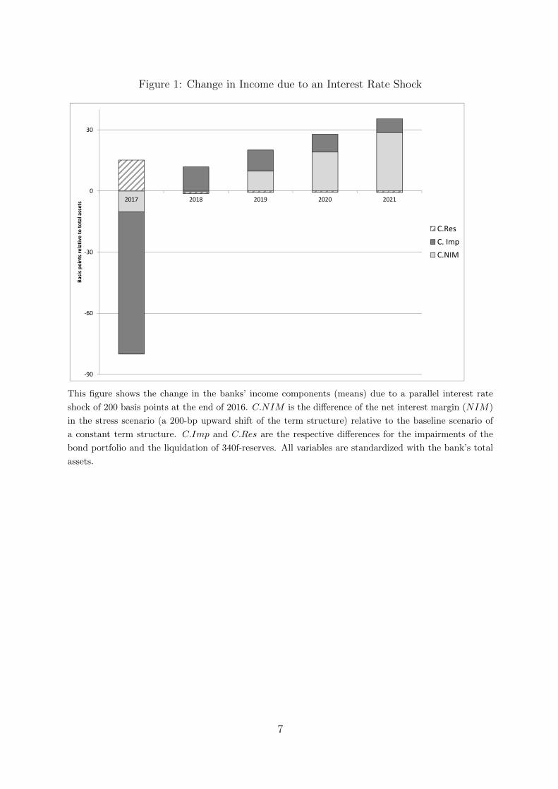
Figure 1: Change in Income due to an Interest Rate Shock

-90

-60

-30

0

30

2017 2018 2019 2020 2021

Ba

sis

po

ints

re

lati

ve

to

to

tal

ass

ets

C.Res

C. Imp

C.NIM

This figure shows the change in the banks’ income components (means) due to a parallel interest rate

shock of 200 basis points at the end of 2016. C.NIM is the difference of the net interest margin (NIM)

in the stress scenario (a 200-bp upward shift of the term structure) relative to the baseline scenario of

a constant term structure. C.Imp and C.Res are the respective differences for the impairments of the

bond portfolio and the liquidation of 340f-reserves. All variables are standardized with the bank’s total

assets.

7

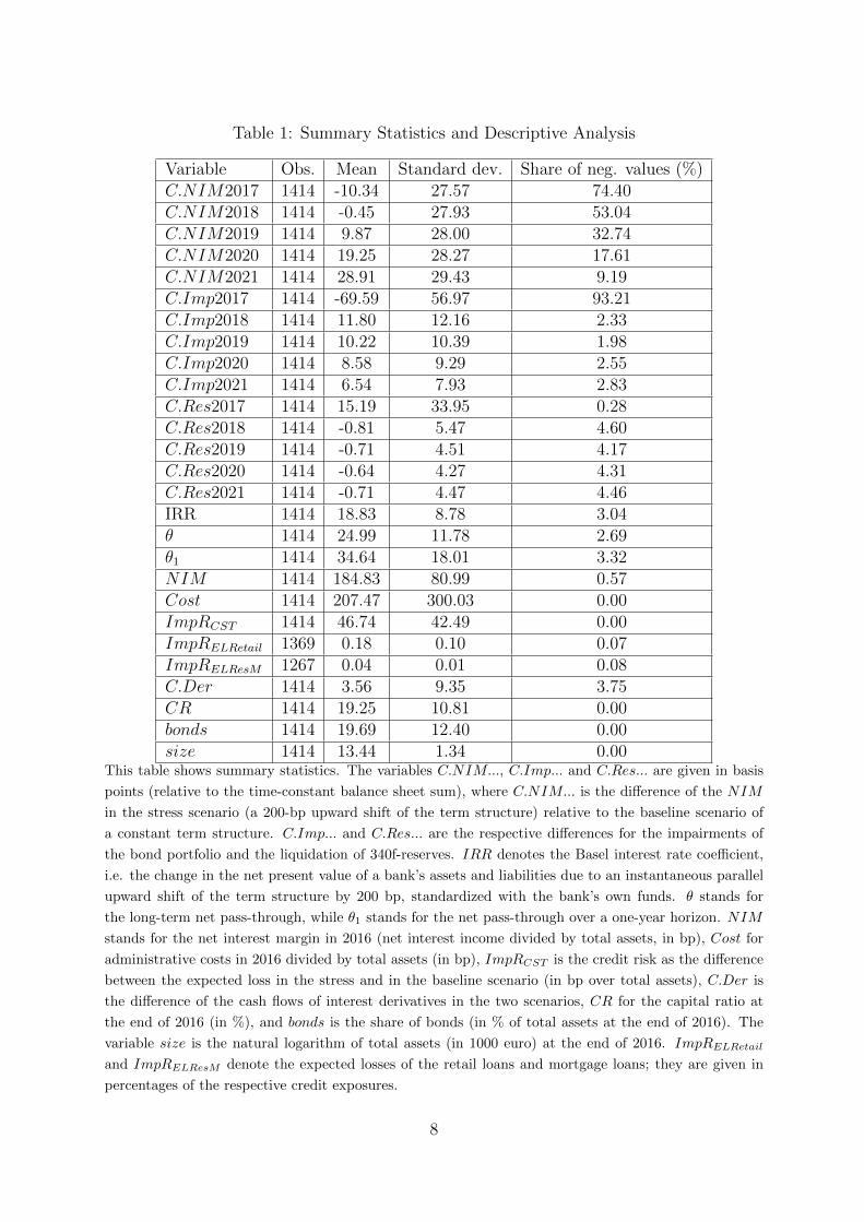
Table 1: Summary Statistics and Descriptive Analysis

Variable Obs. Mean Standard dev. Share of neg. values (%)C.NIM2017 1414 -10.34 27.57 74.40C.NIM2018 1414 -0.45 27.93 53.04C.NIM2019 1414 9.87 28.00 32.74C.NIM2020 1414 19.25 28.27 17.61C.NIM2021 1414 28.91 29.43 9.19C.Imp2017 1414 -69.59 56.97 93.21C.Imp2018 1414 11.80 12.16 2.33C.Imp2019 1414 10.22 10.39 1.98C.Imp2020 1414 8.58 9.29 2.55C.Imp2021 1414 6.54 7.93 2.83C.Res2017 1414 15.19 33.95 0.28C.Res2018 1414 -0.81 5.47 4.60C.Res2019 1414 -0.71 4.51 4.17C.Res2020 1414 -0.64 4.27 4.31C.Res2021 1414 -0.71 4.47 4.46IRR 1414 18.83 8.78 3.04θ 1414 24.99 11.78 2.69θ1 1414 34.64 18.01 3.32NIM 1414 184.83 80.99 0.57Cost 1414 207.47 300.03 0.00ImpRCST 1414 46.74 42.49 0.00ImpRELRetail 1369 0.18 0.10 0.07ImpRELResM 1267 0.04 0.01 0.08C.Der 1414 3.56 9.35 3.75CR 1414 19.25 10.81 0.00bonds 1414 19.69 12.40 0.00size 1414 13.44 1.34 0.00

This table shows summary statistics. The variables C.NIM..., C.Imp... and C.Res... are given in basis

points (relative to the time-constant balance sheet sum), where C.NIM... is the difference of the NIM

in the stress scenario (a 200-bp upward shift of the term structure) relative to the baseline scenario of

a constant term structure. C.Imp... and C.Res... are the respective differences for the impairments of

the bond portfolio and the liquidation of 340f-reserves. IRR denotes the Basel interest rate coefficient,

i.e. the change in the net present value of a bank’s assets and liabilities due to an instantaneous parallel

upward shift of the term structure by 200 bp, standardized with the bank’s own funds. θ stands for

the long-term net pass-through, while θ1 stands for the net pass-through over a one-year horizon. NIM

stands for the net interest margin in 2016 (net interest income divided by total assets, in bp), Cost for

administrative costs in 2016 divided by total assets (in bp), ImpRCST is the credit risk as the difference

between the expected loss in the stress and in the baseline scenario (in bp over total assets), C.Der is

the difference of the cash flows of interest derivatives in the two scenarios, CR for the capital ratio at

the end of 2016 (in %), and bonds is the share of bonds (in % of total assets at the end of 2016). The

variable size is the natural logarithm of total assets (in 1000 euro) at the end of 2016. ImpRELRetail

and ImpRELResM denote the expected losses of the retail loans and mortgage loans; they are given in

percentages of the respective credit exposures.

8

3.5 Descriptive Analysis

In a first step, we look at descriptive analyses of the interest rate shock, especially atthe variables with the C.-operator because, for these variables, we know for sure that theeffect of the increase in the interest level – directly (NIM , Imp, Der) or indirectly (Res)– is the cause for their change as we have the counterfactual of an unchanged interestlevel.The change in net interest income is the effect that first comes to mind when thinkingabout changes in the interest level. However, we see in the summary statistics in Table1 and in Figure 1 that the largest effect by far – at least in the first year after the shock– comes from impairments in the bond portfolio, amounting to almost 70 bp (relative tototal assets) on average in 2017. In the subsequent years (2018-2021), there are write-ups.The net effect due to the impairments in the first year is still negative after five years(32 bp, or 46.7% relative to the impairments in the first year). The impairments in thefirst year are to some degree attenuated by liquidating hidden reserves. This liquidationsoftens the effect by – on average – a bit more than 15 bp (relative to total assets), whichgives a net effect of the impairments of 55 bp (relative to total assets).Looking at the mean of the difference in the net interest margins C.NIM... for the differ-ent years, we see an upward trend from around -10 bp to 29 bp (relative to total assets),meaning that an increase in the interest level is – after some time – beneficial for thebanks. The average difference in the net interest margins is negative in 2017 and slightlynegative in 2018, but strongly positive in 2019 and thereafter, i.e. between 2018 and 2019the effect turns from negative to positive. This is in line with Busch, Drescher, and Mem-mel (2017), who analyzed the data of the corresponding survey of 2015 as to the questionof dynamic versus constant balance sheets, and with Table 2, where – for the median bank– the last year without improvement in the net interest margin is 2018. In Busch andMemmel (2017), the time span during which rising interest levels have a negative impacton the net interest margin is 1.5 years, compared to more than 2 years in this survey.The different time spans may result from different assumptions as to bank management’sreactions: Whereas the time span in Busch and Memmel (2017) is estimated under theassumption that banks can also adjust their balance sheet, the assumption in this surveyis a constant balance sheet. The sum over the period of five years of the difference in thenet interest margins is 47 bp. Hence, as to the net interest margin, the overall effect ofan increase in the interest rate level is positive (for the average bank).Table 2 states the last year (in Appendix A, this horizon is denoted as t∗) where a bank’snet interest margin in the scenario of an upward shift of the term structure relative tothe baseline scenario of a constant term structure is negative or zero (and consequentlypositive in previous years). It only encompasses banks for which the net interest mar-gin (relative to the scenario of a constant term structure) monotonically increases in theperiod 2017-2021, i.e. the net interest margin (relative to the baseline scenario of a con-stant term structure) of 2017 is less than or equal to the one of 2018 and so forth. Themonotonicity is given for 1183 banks out of 1414 banks (share of 83.6%). For instancein the case where 2018 is the ”[l]ast year without improvement”, there are 271 bankswhere the net interest margin (relative to the baseline scenario) in 2018 is negative (orzero) and positive (or zero) from 2019 on. The highest number of banks (299, or 25.27%)experience a deterioration of their net interest margin only in 2017 and, from 2018 on,

9

Table 2: Dynamics of Net Interest Margins

Year Last year without improvement IRRNumber of banks Share (in %) (average)

2016 258 21.81 15.362017 299 25.27 18.722018 271 22.91 20.392019 192 16.23 22.492020 101 8.54 23.362021+ 62 5.24 23.13sum 1183 100.00 19.61

This table shows the last year, in the scenario of a 200-bp upward shift of term structure, in which no

improvement of a bank’s net interest margin manifests (compared to the scenario of a constant term

structure). Only banks whose net interest margin dynamics in the period 2017-2021 are monotonically

increasing are considered (1183 out of 1414, which equals 83.6%).

an improvement of their net interest margin relative to the baseline scenario. However,there are banks that have lower net interest margins (relative to the baseline scenario)even after five years (62 banks).The year with the turning point, i.e. the last year without improvement and the follow-ing year with the improvement, shows considerable variation, reaching from immediateimprovement to five years or more after the interest shock took place. Moreover, whenlooking at the third column of Table 2, where the mean exposure to interest rate risk(measured by the Basel interest rate risk coefficient at the end of 2016) of the respectivegroup of banks is given, it seems as if the exposure to interest rate risk (IRR) is relatedto the speed of improvement: The exposure to interest rate risk (IRR) is positively as-sociated with the length of the time span (t∗) with no improvement concerning the netinterest margin. This is in line with the rather mechanical model in Appendix A (seeEquations (22) and (23)).

4 Risk Management

4.1 Tactical Risk Exposure

In the short run, when faced with valuation losses in the bond portfolio, banks can takedifferent measures to attenuate the impact on the profit and loss statement, for instancethey can liquidate a special kind of hidden reserves (340f-reserves) or they can reclassifytheir bonds from Umlaufvermogen (current assets) to Anlagevermogen (fixed assets) (seeSubsection 3.2). However, we employ data which were generated applying the assumptionof a static balance sheet and, therefore, reclassification is not permitted. Besides, as theinterest rate shock in this survey is assumed to be permanent, the reclassification of thebonds is not an option because, in the event of a permanent shock, bonds classified asAnlagevermogen also have to be written down.To investigate the relationship between the liquidation of reserves and the impairment

10

Table 3: Change in Reserves

Variables C.Res2017 C.Res2018 C.Res2019 C.Res2020 C.Res2021C.Imp -0.245*** -0.079*** -0.075*** -0.067*** -0.049**

(0.027) (0.023) (0.021) (0.021) (0.022)size 0.316 -0.119 -0.076 -0.064 0.086

(0.621) (0.090) (0.071) (0.075) (0.090)CR 0.109** -0.009 -0.007 -0.006 -0.004

(0.052) (0.007) (0.006) (0.006) (0.005)const. -8.207 1.893 1.208 0.916 -1.468

(9.067) (1.306) (1.053) (1.121) (1.314)R-sq 0.169 0.031 0.030 0.021 0.009Nobs 1414 1414 1414 1414 1414

This table shows the estimation results of Equation (1) for different years; robust standard deviations in

brackets; *** and ** denote significance levels of 1% and 5%. R − sq is the coefficient of determination

R2 and Nobs is the number of observations.

losses in the bond portfolio, we run the following regression:

C.Rest,i = αt + βt · C.Impt,i + γ′tXi + εt,i, (1)

where Impt,i is bank i’s impairment of the values of bonds (divided by the bank’s to-tal assets) in year t, Rest,i is the amount of liquidated hidden reserves on bonds (dividedby the bank’s total assets) in year t = 2017, ..., 2021, where the C. operator states thatwe use the difference of the respective variables in the shock scenario (a sudden rise inthe interest level) and the baseline scenario (constant term structure). This allows us toexclusively look at the effect due to an increase in the interest level. Xi is a vector thatcontains the control variables sizei and capital ratio (CRi). β2017 can be interpreted asthe euro amount of immediately liquidated hidden reserves as a consequence of an interestrate shock that leads to one euro of impairments in the bond portfolio.As stated above, we expect that the negative impact on the P&L through higher impair-ments after a positive shock in the interest rate will be attenuated by the liquidation ofreserves. Thereby, we expect that a reduction in the difference for impairments in the+200-bp scenario versus the scenario with the constant term structure (higher negativeeffect on P&L) will be associated with an increase in the difference in reserve flows inthe +200-bp scenario versus the scenario with the constant term structure. Hence, weexpect a negative βt in Equation (1) where we show the results of this equation in Table3. Especially in the first year, we observe a highly significant and negative estimate witha coefficient of determination of almost 17%. This estimate can be interpreted such thatan impairment of one euro leads to 24.5 cents of immediate liquidation of 340f-reserves.As to credit risk, banks are allowed to use these hidden reserves as well. However, ourdata do not make it possible to quantify the usage in this case.

Note that from 2018 on, the banks on average build reserves (instead of liquidatingthem). The sign of the respective coefficients remains negative although the change inreserves alters its sign (see Table 1). This is so because, from 2018 on, there are on averageno longer write-downs in the bond portfolio, but write-ups due the pull-to-par effect.

11

Table 4: Impairments

Variables C.Imp2017 C.Imp2018 C.Imp2019 C.Imp2020 C.Imp2021IRR -1.224*** 0.223*** 0.204*** 0.197*** 0.149***

(0.171) (0.048) (0.043) (0.042) (0.038)bonds -2.546*** 0.462*** 0.404*** 0.331*** 0.274***

(0.139) (0.039) (0.034) (0.032) (0.027)size 4.900*** 0.114 0.007 -0.092 -0.114

(0.981) (0.200) (0.171) (0.158) (0.131)CR -0.157* 0.011 0.001 -0.003 -0.012

(0.085) (0.040) (0.040) (0.040) (0.041)const. -59.253*** -3.237 -1.709 -0.340 0.115

(13.647) (2.872) (2.496) (2.299) (1.912)R-sq 0.443 0.297 0.318 0.285 0.261Nobs 1414 1414 1414 1414 1414

This table shows the estimation results of Equation (2) for different years; robust standard deviations in

brackets; *** and * denote significance levels of 1% and 10%. R − sq is the coefficient of determination

R2 and Nobs is the number of observations.

The amount of impairments as a consequence of the interest rate shock C.Impt,i in abank’s bond portfolio is likely to depend on this bank’s exposure (IRRi) to interest raterisk and the size (bondsi) of its bond portfolio:

C.Impt,i = αt + β1,t · IRRi + β2,t · bondsi + γ′tXi + εt,i (2)

As said above, the variable IRRi denotes the Basel interest rate coefficient under a+200 basis points shock, that is, the present value loss in the valuation of fixed assetsgiven a sudden parallel increase in the yield curve by 200 bp, divided by the regulatoryown funds of the bank. As stated in Subsection 3.3, we use this as a proxy for the bank’sexposure to interest rate risk, which is a common assumption (see, for instance, DeutscheBundesbank (2015)).As to the explanation of the impairments of the bond portfolios, we show the resultsof estimating Equation (2) in Table 4. These results are important for top-down stresstesting, because, as explanatory variables, only information is used that is available beforethe stress tests and that is part of the normal supervisory reporting. According to theseresults, a bank’s exposure to interest rate risk (IRR) and the size of its bond portfolio(bonds) are important determinants for its write-downs in the bond portfolio. Not onlyare the coefficients highly significant, but the explained variation, especially in the firstyear, is remarkably high at more than 44%.

In principle, a bank could be exposed to interest rate risk without many bond holdings.For instance, a bank could invest into loans with a long fixed-interest period (instead of:into corresponding bonds). This would reduce the impairments resulting from a rise inthe interest level because a loan only has to be written down if the creditworthiness ofthe borrower deteriorates, but not (unlike a bond) if the risk-free interest rate increases(see Subsection 3.2). Not to use bonds as a liquidity reserve requires elaborate riskmanagement, which, we hypothesize, could consist in the holding of derivatives to manage

12

the exposure to interest rate risk. To investigate whether banks with more instrumentsto adjust their risk profile have different impairments in their bond portfolio, we run thefollowing regression (for 2017):

C.Impi = α+αD ·Di+β1·IRRi+β1,D ·IRRi·Di+β2·bondsi+β2,D ·bondsi·Di+γ′Xi+εi (3)

where Di is a dummy variable that takes the value of one if bank i uses interestderivatives.

Questions as to the usage of interest derivatives (Equation (3)) are treated in this sub-section with the short-term measures, although, for about 80% of the banks (507 out of626 banks), their on-balance sheet net interest income and the cash flows of their interestderivatives move in opposite directions in the event of an interest rate shock. If the usageof interest derivatives were solely a means of fine-tuning risk exposures, we would observethat about 50% of the cash flows of the derivative position move in sync and about 50%of the cash flows move in opposite directions. Nevertheless, we count the usage of theinterest derivatives among the short-term measures because – once the decision to usederivatives has been made – the exact position of the derivatives can be adjusted in nextto no time.In Table 5, the results of Equation (3) are shown. This equation makes it possible to inves-tigate whether the relationship between the impairments Imp in a bank’s bond portfolioand its exposure to interest rate risk and the size of its bond portfolio depends on theusage of interest derivatives. As can be seen from the F − test, which tests whetherthe three coefficients βD, γD and αD in Equation (3) are jointly zero, this relationship ishighly significantly different. When calculated at the respective means of the exposureto interest rate risk (IRR), of the relative size of the bond portfolio (bonds) and of thecontrol variables (see Table 1), the expected impairment after the shock in the interestlevel by 200 bp is 81 bp (relative to the bank’s total assets) and 55.2 bp (relative to thebank’s total assets) for banks without derivatives and with derivatives, i.e. banks withinterest derivatives have on average 25.8 bp lower impairments in their bond portfolio, ofwhich 15.3 bp are due to bank characteristics (other than the usage of derivatives) and10.5 bp are due to the usage of derivatives.A possible explanation of this latter result is that banks with interest derivatives canbetter steer their interest rate risk and liquidity risk so that they can invest a larger partof their assets into illiquid loans (that are not written down in the event of an interestrate shock, but only in the event of deteriorating creditworthiness of the borrowers (seeSubsection 3.2)). This estimate is backed up when we look at the results of a regressionthat explains the loan share loans:5

loans = 41.851 + 5.937 ·D + 0.060 ·NIM − 0.001 · IRR + 0.865 · size− 0.369 · CR + ε

(11.139) (0.940) (0.029) (0.068) (0.475) (0.127) (4)

The loan share loans (relative to the bank’s total assets) is significantly larger forbanks which use interest derivatives (dummy variable D), almost 6 percentage points. Bycontrast, the exposure to interest rate risk IRR does not seem to be related to the size of

5Robust standard errors in brackets; R2 of the cross-sectional regression amounts to 22.61%.

13

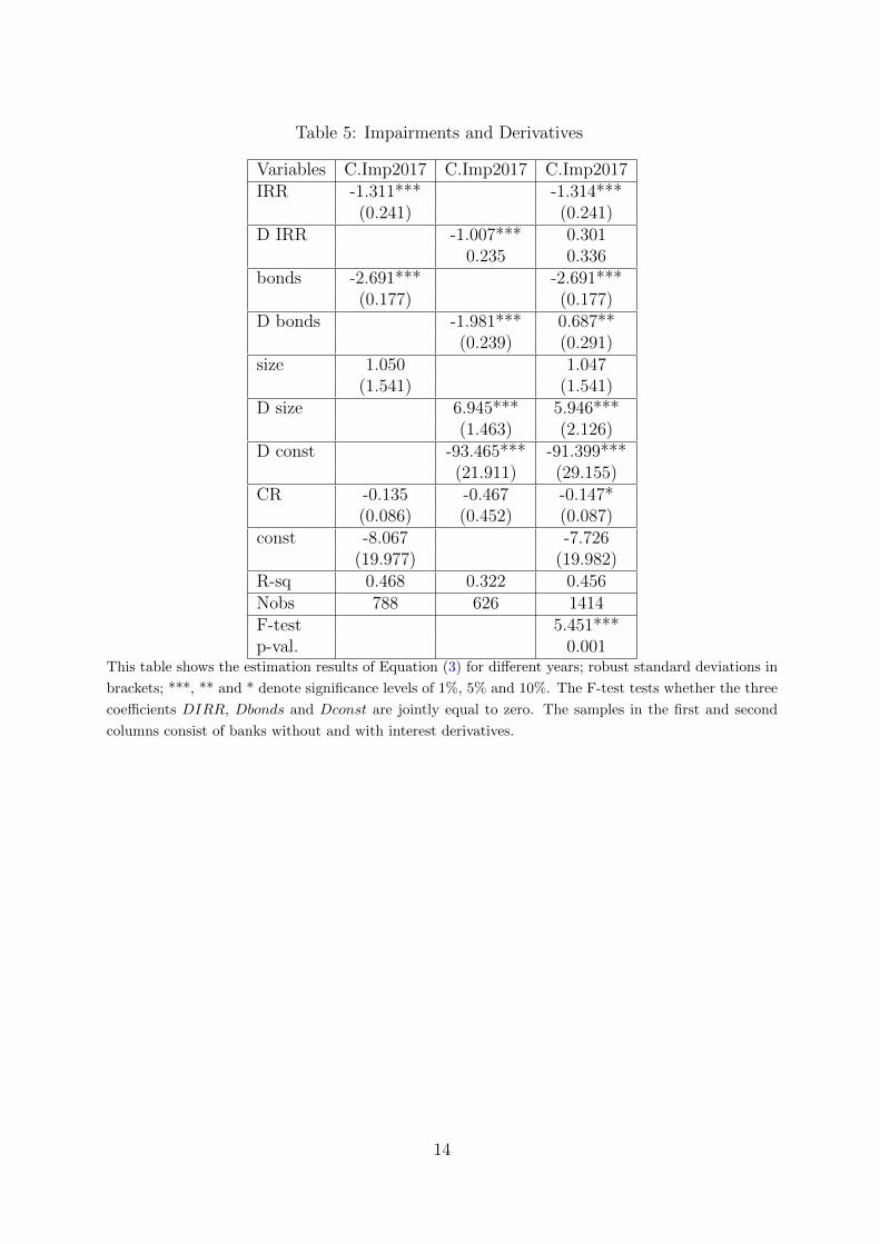
Table 5: Impairments and Derivatives

Variables C.Imp2017 C.Imp2017 C.Imp2017IRR -1.311*** -1.314***

(0.241) (0.241)D IRR -1.007*** 0.301

0.235 0.336bonds -2.691*** -2.691***

(0.177) (0.177)D bonds -1.981*** 0.687**

(0.239) (0.291)size 1.050 1.047

(1.541) (1.541)D size 6.945*** 5.946***

(1.463) (2.126)D const -93.465*** -91.399***

(21.911) (29.155)CR -0.135 -0.467 -0.147*

(0.086) (0.452) (0.087)const -8.067 -7.726

(19.977) (19.982)R-sq 0.468 0.322 0.456Nobs 788 626 1414F-test 5.451***p-val. 0.001

This table shows the estimation results of Equation (3) for different years; robust standard deviations in

brackets; ***, ** and * denote significance levels of 1%, 5% and 10%. The F-test tests whether the three

coefficients DIRR, Dbonds and Dconst are jointly equal to zero. The samples in the first and second

columns consist of banks without and with interest derivatives.

14

the customer loan portfolio, suggesting that customer loans do not have a different interestrate exposure than the rest of the assets. Note that these results are not necessarily basedon causal effects, but are derived from a correlation analysis. An example may illustratethis point: for the variable NIM , the net interest margin, we observe a significantly pos-itive relationship to the loan share loans. From an economic point of view, it is unclearwhether the higher net interest margin NIM is due to better earning opportunities fromgranting customer loans loans or whether an unobservable third factor, for instance aprosperous economic environment in the region where the bank operates, is responsiblefor a high net interest margin NIM and – at the same time – for a large portfolio ofcustomer loans.The result according to which banks with usage of interest derivatives have lower im-pairment losses in their bond portfolio indicates that the hedging of interest rate risk isnot a pure redistribution of this risk from one bank to another bank (if both contractuaylparties are banks). Instead, the result suggests that there are banks that are better suited(for instance banks that use interest derivatives) than others.

4.2 Strategic Risk Exposure

In the long-run perspective, banks can adjust their business environment to some extent.Some parameters can be adjusted more easily than others. One parameter that is pre-sumably difficult to adjust is a bank’s long-term net pass-through (the long-term effect ofa change in the interest level on a bank’s net interest margin; in our study denoted as θ)because it depends on the bank’s business model and this cannot be easily changed. Forinstance, a bank with a traditional business model, i.e. of granting customers loans andtaking in deposits, is likely to have a significantly positive long-term net pass-through θ,i.e. in the event of an increase in the interest level, this bank’s net interest margin largelyimproves. By contrast, an investment bank that buys and issues bonds is likely to have anet pass-through in the long term that is close to zero.Memmel (2018) derives the following relationship between a bank’s difference in its netinterest margin (NIMt,i) in the scenario with a upward shift of the term structure rela-tive to the scenario with a constant term structure, the net long-run pass-through (θi) ofassets and liabilities and its exposure to interest rate risk (IRRi) (see also Appendix A,Equation (17)):

C.NIMt,i = β1,t · θi + β2,t · IRRi + εi (5)

where β1,t and β2,t are positive and negative parameters, respectively. The intuitionbehind this relationship is that a bank’s net interest margin (NIM) usually benefitsfrom a higher interest level (see Busch and Memmel (2017) and Claessens, Coleman, andDonnelly (2018)). This is so because the long-run pass-through on the asset side is usuallygreater than on the liability side, where the extent of the net effect is measured by thevariable θ. Again, we refer to the extreme case of a simplified central bank where its assets– loans to banks – are closely tied to the (short-term) interest level and its liabilities –mostly banknotes – are not remunerated at all, irrespective of the interest level. In thiscase, the long-run net pass-through θ would be one, meaning that an increase in theinterest level by 100 bp leads to an increase in the net interest margin by 100 bp as well.As to the exposure to interest rate risk IRR, it can be seen as a measure of the difference

15

in the fixed-interest periods on the asset and on the liability side. If this difference is large,i.e. the exposure to interest rate risk IRR is high, there is a significantly smaller share ofnew business (which is adjusted to the new interest level) on the asset side than on theliability side so that it takes longer until a rise in the interest level leads to an improvementin the net interest margin NIM (see Appendix A for a model), which explains that thecoefficients β2,t are negative.In this study, having at hand a unique data set on interest rates for a large sample ofbanks, we are able to further analyze the variable θ. More precisely, for each bank i, wecan distinguish between a short-run pass-through in the first year, based on the (non-)repricing of maturing (and existing) business (θ1,i), and a long-term pass-through (θi).Basically, the definitions of both variables are

θi =∑

j sgnjptjwij , (6)

θ1,i =∑

j sgnjptijwij , (7)

where the sum goes over all interest-bearing asset and liability positions j, sgnj = 1 ifposition j is on the asset side and sgnj = −1 if position j is on the liability side, and wijdenotes the weight of position j in the respective bank. The difference between the twodefinitions lies in the variable pt: While ptj is an average pass-through per balance sheetposition as derived in Memmel (2018), in this study, we have the possibility of extractingthe bank-individual pass-through in a one-year horizon ptij. Thus, any variation in θ1does not only stem from different balance sheet compositions, but also from different(bank-individual) pass-throughs. It is interesting (but not unexpected) that the standarddeviation of θ1 is much larger than that of θ, however, a different dataset was used forcalculating both variables. When testing whether the variability of θ1 is mainly drivenby wij or ptij, it turns out that for a given balance sheet position j, the variation ofptij is much larger than for wij. This means that the variation of the pass-through ismuch greater than the variation of the balance sheet composition – this result may beconsidered surprising. As to the origin of the variation, as noted above, one key may lie inthe level of competition in the market in which a bank operates (see Heckmann-Draisbachand Moertel (2019)). There is empirical evidence that the bank-individual pass-throughdepends on the degree of competition a bank experiences (see Heckmann-Draisbach andMoertel (2019)). However, this question is not in the focus of the current analysis. In allanalyses, we use both definitions of θ and are able to shed some light onto the variationof this variable.In Tables 6 and 7, the results of Equation (5) are displayed, where the control variablesCR and size have been additionally included (consistent with the previous section) andthe two different versions of θ and θ1 are used in the respective tables.

It turns out that for both definitions of θ, both variables of interest, i.e. θ or θ1, the netpass-through, and IRR, the bank’s exposure to interest rate risk, are highly significantwith the predicted sign. Whereas the coefficient for IRR is around -1 for all horizons,we observe an increase for the variables θ and θ1, which is in line with the derivation inMemmel (2018) where the coefficient for θ is equal to the share of liabilities that havealready matured by the year t. The coefficient of determination, R2, amounts to about17% for all horizons, when using θ. For θ1, however, the value of R2 increases with an

16

Table 6: Difference of Net Interest Margins in the Scenarios

Variables C.NIM2017 C.NIM2018 C.NIM2019 C.NIM2020 C.NIM2021θ 0.220*** 0.499*** 0.666*** 0.806*** 0.947***

(0.076) (0.077) (0.081) (0.082) (0.085)IRR -1.289** -1.286*** -1.193*** -1.050*** -0.890***

(0.164) (0.159) (0.154) (0.152) (0.152)size 0.460 1.115* 1.389** 1.475** 1.304

(0.683) (0.669) (0.662) (0.662) (0.684)CR 0.145 0.114 0.094 0.071 0.064

(0.142) (0.132) (0.128) (0.126) (0.125)const. -0.543 -5.876 -4.801 -2.321 3.238

(12.040) (11.745) (11.521) (11.482) (11.787)R-sq 0.169 0.176 0.175 0.171 0.167Nobs 1414 1414 1414 1414 1414

This table shows the estimation results of Equation (5) for different years when using θ as defined in

Equation (6); robust standard errors; ***, ** and * denote significance levels of 1%, 5% and 10%. R− sqis the coefficient of determination R2 and Nobs is the number of observations, respectively.

Table 7: Difference of Net Interest Margins in the Scenarios

Variables C.NIM2017 C.NIM2018 C.NIM2019 C.NIM2020 C.NIM2021θ1 0.257*** 0.411*** 0.525*** 0.619*** 0.723***

(0.077) (0.076) (0.075) (0.075) (0.077)IRR -1.322*** -1.290*** -1.188*** -1.037*** -0.874***

(0.142) (0.138) (0.134) (0.132) (0.133)size -0.146 -0.014 -0.085 -0.285 -0.757

(0.667) (0.653) (0.653) (0.645) (0.658)CR 0.153 0.146 0.140 0.127 0.131

(0.133) (0.121) (0.112) (0.106) (0.101)const. 4.664 6.975 12.507 18.721 27.963**

(12.832) (12.508) (12.272) (12.040) (12.075)R-sq 0.187 0.203 0.213 0.216 0.224Nobs 1414 1414 1414 1414 1414

This table shows the estimation results of Equation (5) for different years when using the one-year net

pass-through θ1 as defined in Equation (7). Robust standard errors; ***, ** and * denote significance

levels of 1%, 5% and 10%. R − sq is the coefficient of determination R2 and Nobs is the number of

observations, respectively.

17

increasing horizon.Given some assumptions (not necessarily those in Appendix A), the relationship in

Equation (5) should be valid. However, without data about the difference in the NIMin different scenarios, this relationship cannot be tested, at least not in a direct way.For instance, as Memmel (2018) had no data about the differences in the banks’ netinterest margins in the different scenarios (C.NIMt,i), he could only indirectly test thisrelationship. He further assumes that banks try to stabilize their future net interestincome, i.e. to minimize the variance of C.NIMt,i,

minIRRi

var (C.NIMt,i) = (β1,t · θi + β2,t · IRRi)2 var(∆R) + σ2

ε (8)

Taking θi as given and only being able to vary the exposure IRRi to interest raterisk, he obtains a relationship between θi and IRRi, namely that these two variables areassociated in a positive way. In other words: If we further assume that bank managementtries to stabilize the net interest margin in the mid-term by optimizing the exposure tointerest rate risk (IRR), we will observe a positive relationship between a bank’s interestrate risk exposure IRR and its long-term net pass-through θ, i.e. that β1 in Equation (9)is positive.

As a further focus of our study, we analyze the interdependence of interest rate riskand credit risk. It is empirically documented that banks have an internal risk budgetwhich they allocate to interest rate risk (IRRi) and credit risk (ImpRCST,i) (see Schrandand Unal (1998) and Memmel (2018)).

To test the validity of the behavioural assumptions, i.e. variance minimization offuture net interest margins as in Equation (8) and a joint risk budget, we run the followingregression:

IRRi = α + β1 · θi + β2 · ImpRCST,i + γ′Xi + εi. (9)

As a measure for credit risk ImpRCST,i, we use in this case the expected loss for 2017under the stress scenario and substract the expected loss without stress. We think this isa good measure for credit risk in this context because this measure gives the additionalcredit losses in the stress test. We expect β1 and β2 to be positive and negative, respec-tively. Although the relationship in Equation (9) is rather mechanical and involves littleeconomic reasoning, it is not always the case that it empirically holds: Banca d’Italia(2013) finds for a sample of 11 Italian banks that there is only a weak link between abank’s exposure to interest rate risk and the change in its net interest income given aninterest rate shock, which may be due to relatively low interest rate risk exposure of thebanks in the sample.In Table 8, first column, we find evidence for the reasoning according to which bankstry to stabilize their net interest margin: The coefficient in front of θ is highly positivelysignificant. More specifically, the coefficient for θ is larger (by nearly a factor of 2) thanthe coefficient for θ1. This means that the long-term net pass-through is a stronger deter-minant of the exposure to interest rate risk than the short-term (one-year) pass-through.In addition, we see that the exposure to credit risk and to interest rate risk are negativelyassociated, where the coefficients vary slightly in the two different specifications, from-0.026 to -0.023. This suggests that banks have a risk budget which they allocate eitherto credit risk or to interest rate risk. These findings are in line with Schrand and Unal(1998) and Memmel (2018). Note that the exposures to interest rate risk and the exposure

18

Table 8: Determinants of IRR and NIM

Variables IRR IRR NIMIRR 0.187***

(0.049)θ 0.174***

(0.027 )θ1 0.089***

(0.016)ImpR-CST -0.023*** -0.026*** 0.969***

(0.005) (0.005) (0.177)Cost 0.292***

(0.048)CR -0.124*** -0.111*** -0.743***

(0.031) (0.025) (0.193)size -0.302 -0.625*** -8.761***

(0.197) (0.194) (1.099)const. 22.018*** 27.524*** 236.096***

(2.943) (2.763) (22.756)R-sq 0.093 0.074 0.352Nobs 1414 1414 1380

This table shows the estimation results of Equations (9) and (10). Robust standard errors in brackets;

*** denotes a significance level of 1%. R − sq is the coefficient of determination R2 and Nobs is the

number of observations. Observations of the variable Cost that are larger than the median plus five

times the interquartile range are removed.

to credit risk are measured relative to the shock sizes of different stress tests so that thesize of the coefficient cannot be interpreted, only its sign.

As to the level of the net interest margin NIM (and not the differences in the scenariosas above), we hypothesize that banks with high exposure to interest rate risk IRR andhigh credit risk ImpRCST have a high net interest margin NIM , i.e. β1 > 0 and β2 > 0,because interest rate risk and credit risk should be remunerated in the form of a highernet interest margin.

NIMi = α + β1 · IRRi + β2 · ImpRCST,i + β3 · Costi + γ′Xi + εi, (10)

In Equation (10), we additionally include the variable Cost, which gives the bank’sadministrative costs. We do so because these variables are found in the literature toimpact the net interest margin (see, for instance, Saunders and Schumacher (2000) andBusch and Memmel (2016)).In Table 8, third column, the results of the corresponding regression (10) are displayed.We see that banks with more interest rate risk IRR and more credit risk have a signifi-cantly higher net interest margin NIM . However, as to the credit risk, it is unclear fromthis result whether the increase in the banks’ net interest margin (NIM) only covers theexpected losses or (additionally) a risk premium. Below, we will come back to this issue.In addition, the variable Cost as a proxy for the services a bank provides is positively

19

significant: Banks with one euro more of administrative costs have – ceteris paribus –about 30 cents more of net interest income, when comparing institutions with the samebalance sheet sum.

Above, we looked at the risk from the whole credit portfolio. In the following, weemploy the richness of our data set and look at more granular data, i.e. at different typesof loans and the corresponding expected losses. Especially, we are interested in the issueof how banks deal with their expected losses in the credit portfolio as to the setting ofbank rates. Expected losses are a cost component of loan granting and this componentshould be reflected in the level of the corresponding bank rates if banks price credit risk(see, for instance, Edelberg (2006) and Magri and Pico (2011)). In order to empiricallycheck the hypothesis of a positive relation between bank rates and credit risk, we estimatethe following relation between the bank rates and the expected loss per exposure amount,i.e. the impairment rate (ImpREL,i,j = LGDi,j · PDi,j), at the exposure class level (j)with bank individual data (i):

IRi,j = α + β1 · ImpREL,i,j + β2 · Costi + γ′Xi + εi,j, (11)

In addition, we estimate the equation above with fixed effects for each bank. Thereby, wecontrol for unobservable bank characteristics. Note that in this analysis, we can includeas control variables in the vector Y only variables that vary across banks’ balance sheetpositions and not only across banks.

IRi,j = αi + β · ImpREL,i,j + γ′Yi,j + δi + εi,j, (12)

Estimating Equation (11) for the two exposure classes retail and loans secured byresidential mortgages, we find that our hypothesis is confirmed (see Table 9, first andsecond columns). Expected credit losses are significantly positively related to bank ratescontrolling for the bank’s administrative costs Cost, its capital ratio CR, its total assetssize, its interest rate risk IRR and the loans’ residual fixed-interest period (fixed-interestperiod). This is especially true for retail loans where additionally the R2 is almost 3percentage points higher than for mortgage loans. It seems as if the low expected lossesof mortgage loans (see Table 1) were not a decisive cost component. In the third columnof Table 9, we report the results of the fixed effects panel regression (12) and find thatthe positive relation between expected losses and bank rates is even more significantlysupported.Turning to the control variables, we find that the capital ratio CR is positively – butinsignificantly – related to the bank rate. One possible explanation for this finding isthat, from a bank’s perspective, capital is relatively costly and the bank will price inthese costs which are reflected in higher bank rates. The finding of an often negativerelation between the loans’ residual fixed-interest period and the bank rate could be dueto the fact that loans with a long fixed-interest period lead to additional income so thatprofit-maximising banks find it optimal to lower the bank rates. This is just the oppositereasoning as with the administrative costs where we observe a positive relation.

As the relationship between an increase in the marginal costs and the corresponding

20

price is not trivial (see Appendix B),6 we generate a new regressor which is equal topti,j times ImpREL,i,j (instead of ImpREL,i,j alone). The variable pti,j gives the pass-through of another cost component, namely the interest level rf , and we assume thatthe pass-through for all cost components is the same for each type of loan a bank offers.For instance, if Bank A increases its rates for mortgage loans (j = 1) by 180 bp aftera shock of 200 bp to the risk-free rate, our assumption states that the pass-throughptA,1=90%=180/200 is the same for each cost component of Bank A’s mortgage loans(expected losses, refinancing, proceeds of bearing interest rate risk, ... ).Controlling for the bank’s administrative costs, its capital ratio, its size, its interest raterisk and the residual fixed-interest period of the loans, we expect that the correspondingcoefficient is one (see Appendix B) if the banks treat all cost components in the sameway, irrespective of their nature (here: expected credit losses and interest level). In orderto test our hypothesis, we estimate the following two equations:

IRi,j = α + β1 · pti,j · ImpREL,i,j + β2 · Costi + γ′Xi + εi,j, (13)

IRi,j = αi + β · pti,j · ImpREL,i,j + γ′Yi,j + εi,j, (14)

When we introduce the variable pt ∗ ImpREL consisting of the pass-through times ex-pected losses as an explanatory variable (instead of the expected losses alone), as suggestedin Equations (13) and (14), (see Table 9, columns four to six), we can quantitatively in-terpret the coefficient in front of this variable (see Appendix B). A coefficient of 1 meansthat expected losses are priced-in in the bank rate in the same way as the risk-free interestrate. If, however, the banks not only price in the expected losses, but a risk premium forthe credit risk as well, then the coefficient β1 in Equation (13) and β in Equation (14)are larger than one. We see that the coefficient in the panel specification (column 6) issignificantly larger than one, hinting that a risk premium is included in the bank rate.

5 Conclusion

In this paper, we use data from a quantitative survey among small and medium-sizedGerman banks to learn about banks’ interest and credit risk management. In the case ofan upward shift of the interest level, we find that most of the reduction in earnings in thefirst year after this shock results from write-downs in the bond portfolio. We also see thatbanks tend to dampen these write-downs by liquidating hidden reserves (about 24 cent foreach euro of write-downs) and that banks which use interest derivatives are less exposedto the risk of write-downs in the bond portfolio. Moreover, we find that interest rate riskand credit risk are remunerated in the sense that banks with more exposure to these risks(ceteris paribus) have higher net interest margins. Looking at more granular data of thecredit portfolio, we see that banks seem to be compensated for the expected losses. Weeven find hints of a risk premium that banks include in their loan rates. In addition,banks seem to stabilize their mid-term net interest margins by exposing themselves to

6Bulow and Pfleiderer (1983) theoretically show that producers pass through less or even more thanthe change in the variable costs and that the extent of the pass-through strongly depends on the functionalform of the demand function.

21

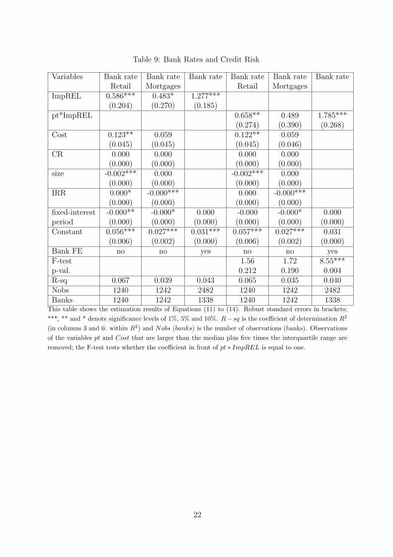
Table 9: Bank Rates and Credit Risk

Variables Bank rate Bank rate Bank rate Bank rate Bank rate Bank rateRetail Mortgages Retail Mortgages

ImpREL 0.586*** 0.483* 1.277***(0.204) (0.270) (0.185)

pt*ImpREL 0.658** 0.489 1.785***(0.274) (0.390) (0.268)

Cost 0.123** 0.059 0.122** 0.059(0.045) (0.045) (0.045) (0.046)

CR 0.000 0.000 0.000 0.000(0.000) (0.000) (0.000) (0.000)

size -0.002*** 0.000 -0.002*** 0.000(0.000) (0.000) (0.000) (0.000)

IRR 0.000* -0.000*** 0.000 -0.000***(0.000) (0.000) (0.000) (0.000)

fixed-interest -0.000** -0.000* 0.000 -0.000 -0.000* 0.000period (0.000) (0.000) (0.000) (0.000) (0.000) (0.000)Constant 0.056*** 0.027*** 0.031*** 0.057*** 0.027*** 0.031

(0.006) (0.002) (0.000) (0.006) (0.002) (0.000)Bank FE no no yes no no yesF-test 1.56 1.72 8.55***p-val. 0.212 0.190 0.004R-sq 0.067 0.039 0.043 0.065 0.035 0.040Nobs 1240 1242 2482 1240 1242 2482Banks 1240 1242 1338 1240 1242 1338

This table shows the estimation results of Equations (11) to (14). Robust standard errors in brackets;

***, ** and * denote significance levels of 1%, 5% and 10%. R− sq is the coefficient of determination R2

(in columns 3 and 6: within R2) and Nobs (banks) is the number of observations (banks). Observations

of the variables pt and Cost that are larger than the median plus five times the interquartile range are

removed; the F-test tests whether the coefficient in front of pt ∗ ImpREL is equal to one.

22

interest rate risk and they act as if they have a risk budget which they either allocate tocredit risk or to interest rate risk.

A Appendix: Exposure to Interest Rate Risk and

the Dynamics of the Net Interest Margin

In this section, we formulate and formalize our expectations concerning the dynamics ofthe net interest margin. We assume a bank with a stylized balance sheet (the assumptionsare similar to Busch and Memmel (2017) and Memmel (2018)): On the asset side, thereare default-free loans (share: θA) that are granted in a revolving manner, i.e. whenever aloan matures, it is replaced by a new one. These loans have a maturity MA and a couponc equal to the then prevailing interest level. The other assets are cash (share: 1 − θA).On the liability side, there are default-free loans (share: θL) with maturity ML that thebanks issues in a revolving manner; the rest of the liabilities consist of non-remuneratedcurrent accounts (share: 1 − θL). Please note that θA (and θL) can also be interpreteddifferently: Instead of the share of assets that have a pass-through of 100%, it can alsobe interpreted as the average pass-through on the asset side. This interpretation is morein line with the use of the variable θ := θA − θL in the main sections of this paper.Given these assumptions and a parallel shift ∆R of the term structure in t = 0, thedifference of the net interest margin (NIM) to the case of no interest rate shock is:

C.NIM = (φAθA − φLθL) · ∆R (15)

where φA and φL denote the share of loans and bonds that have already matured by timet. The interest rate risk (IRR) of such a bank is:

IRR =1

2(MAθA −MLθL) (16)

Combining Equations (15) and (16) and setting t = 1 such that φA = 1/(2 ·MA) andφL = 1/(2 ·ML) (see Busch and Memmel (2017)), we obtain

C.NIM

∆R=

(φL +

1

2 ·MA

)θ − 1

MA ·ML

IRR. (17)

More generally, we have for Mk > 1 with k = A,L:

φk(t) =

t/2Mk

if t ≤ 1t−1/2Mk

if 1 < t < Mk + 1/2

1 if t ≥Mk + 1/2

(18)

We thus expect that the temporal development of the net interest margin in the shockscenario, compared to the case of no shock, depends in a characteristic way on the averagematurities of the asset and liability side, respectively. Of course, we do not expect a realbank to have a business model and a balance sheet as simple as in our assumptions.However, since the data contains information on the average maturity, we check whetherthe prediction of our model is in line with this information. Indeed, when evaluating the

23

temporal evolution of C.NIM for groups of banks with different average maturities, weobserve that the higher ML, the smaller is the increase of C.NIM from 2017 to 2021. Forbanks with 0.5y < ML < 1.5y, the increase 42.7 basis points (relative to the balance sheetsum), while it is only 23.7 bp for banks with ML > 4.5y. For different buckets of MA, weobserve that the increase of C.NIM is higher with increasing MA. These results indicatethat, despite the simplicity of the model, our formulation of the temporal development ofC.NIM captures some important features of the real dynamics of the net interest margin.

For 1 < ML < t− 1/2 < MA, Equation (15) becomes

C.NIM

∆R=t− 1/2

MA

θA − θL. (19)

Equation (16) can be transformed to

MA =2 · IRR +MLθL

θA. (20)

Combining Equations (19) and (20), we obtain

C.NIM

∆R=

(t− 1

2

)θ2A

2 · IRR +MLθL− θL. (21)

Let t∗ be the horizon, for which C.NIM = 0 in Equation (21), i.e. the horizon where thenegative effect of an increase in the interest level ends and the positive effect starts:

0 =

(t∗ − 1

2

)θ2A

2 · IRR +MLθL− θL. (22)

One can show (applying the theorem about implicit functions) that this horizon increasesif the interest rate risk goes up:

∂t∗

∂IRR=

2

2 · IRR +MLθL> 0 (23)

This is line with the results shown in Table 2.

B Appendix: Loan Rate and Expected Losses

In this appendix, we want to outline our idea of how to establish a relationship betweenthe bank rate and the expected losses. We start with three examples that show that banksmaximising their profits choose the extent of the pass-through depending on the marketsituation and that, however, the relationship between market power and the pass-throughis not monotone (see Bulow and Pfleiderer (1983) on whom our examples are based).In the first example, we assume a bank that faces demand D for loans according to thedemand function D(IR) = a− b · IR, where IR is its loan rate and a and b are (positive)parameters. Concerning loan granting, the bank has variable costs c. Maximising its

24

profits Π = D(IR) · (IR− c), it sets its loan rate IR∗M to

IR∗1 =a

2b+c

2(24)

In the second example, we assume a bank that faces a demand curve with constantelasticity −η > 1: D(IR) = b · IRη. Profit maximization implies

IR∗2 = c · η

η + 1(25)

By contrast (third example), a bank facing perfect competition will set its loan rate IR∗3equal to the variable costs c:

IR∗3 = c (26)

These three examples show that banks with market power may pass on less (∂IR∗1/∂c =1/2) or more (∂IR∗2/∂c = η/(η+1) > 1) than the actual change in the marginal costs andthat banks without market power (∂IR∗3/∂c = 1) pass on the entire change in marginalcosts.To circumvent the problem of the differing (and non-monotonic) pass-throughs, we makeuse of our rich data set: We know the pass-through for the loan rate IR∗i with respectto one cost component, namely with respect to changes in the risk-free interest rate rf ,denoted by pti = ∂IR∗i /∂rf . We assume that the pass-through for other cost componentsis the same for the same bank i, for instance for the expected losses ImpREL,i:

pti :=∂IR∗i∂rf

=∂IR∗i

∂ImpREL,i

(27)

Under this assumption, we can express the change in bank i’s loan rate as

∆IR∗i = pti · ∆ImpREL,i. (28)

In our data, there are the bank rates IRi,j for different asset classes j, the correspond-ing pass-throughs pti,j for a change in the interest level and the expected rate of lossesimpREL,i,j. This may lead to the following empirical relationship:

IRi,j = α + β · (pti,j · ImpREL,i,j) + εi,j (29)

which corresponds to Equations (13) and (14) in the main text. If the assumptions fromabove hold, we expect the variable β to equal one. If not only the expected losses, butalso a risk premium is priced-in, then β is larger than one. Note that the pass-throughpti,j is derived from the observations for the same bank in two different scenarios, whereaswe use the cross-sectional variation for the estimation of regression (29).

References

Angbazo, L. (1997). Commercial bank net interest margins, default risk, interest rate riskand off balance sheet activities. Journal of Banking and Finance 21, 55–87.

25

Banca d’Italia (2013). Financial Stability Report. Number 6/2013.

Bornemann, S., T. Kick, C. Memmel, and A. Pfingsten (2012). Are banks using hiddenreserves to beat earnings benchmarks? Evidence from Germany. Journal of Banking &Finance 36, 2403–2415.

Brewer, E., B. A. Minton, and J. T. Moser (2000). Interest rate derivatives and banklending. Journal of Banking and Finance 24, 353–379.

Bulow, J. I. and P. Pfleiderer (1983). A note on the effect of cost changes on prices.Journal of Political Economy 91(1), 182–185.

Busch, R., C. Drescher, and C. Memmel (2017). Bank stress testing under differentbalance sheet assumptions. Discussion Paper 07/2017, Deutsche Bundesbank.

Busch, R. and T. Kick (2015). Income structure and bank business models: Evidence onperformance and stability from the German banking industry. Schmalenbach BusinessReview 67, 226–253.

Busch, R. and C. Memmel (2016). Quantifying the components of the banks’ net interestmargin. Financial Markets and Portfolio Management 30(4), 371–396.

Busch, R. and C. Memmel (2017). Banks’ net interest margin and the level of interestrates. Credit and Capital Markets 50(3), 363–392.

Claessens, S., N. Coleman, and M. Donnelly (2018). ”Low-For-Long” interest rates andbanks’ interest margins and profitability: Cross-country evidence. Journal of FinancialIntermediation 35, 1–16.

Deutsche Bundesbank (2015). Financial Stability Review 2015.

Drechsler, I., A. Savov, and P. Schnabl (2018). Banking on deposits: Maturity transfor-mation without interest rate risk. CEPR Discussion Paper No. DP 12950.

Edelberg, W. (2006). Risk-based pricing of interest rates for consumer loans. Journal ofMonetary Economics 53, 2283–2298.

Heckmann-Draisbach, L. and J. Moertel (2019). Hampered monetary policy transmission- a supply side story? mimeo.

Hoffmann, P., S. Langfield, F. Pierobon, and G. Vuillemey (2018). Who bears interestrate risk? European Central Bank Working Paper No 2176.

Magri, S. and R. Pico (2011). The rise of risk-based pricing of mortgage interest rates inItaly. Journal of Banking and Finance 35, 1277–1290.

Memmel, C. (2014). Banks’ interest rate risk: the net interest income perspective versusthe market value perspective. Quantitative Finance 14, 1059–1068.

Memmel, C. (2018). Why do banks bear interest rate risk? Schmalenbach BusinessReview 70 (3), 231–253.

26

Purnanandam, A. (2007). Interest rate derivatives at commercial banks: An empiricalinvestigation. Journal of Monetary Economics 54, 1769–1808.

Saunders, A. and L. Schumacher (2000). The determinants of bank interest margins: Aninternational study. Journal of International Money and Finance 19, 813–832.

Schrand, C. and H. Unal (1998). Hedging and coordinated risk management: Evidencefrom thrift conversions. The Journal of Finance 53 (3), 979–1013.

Sierra, G. E. and T. J. Yeager (2004). What does the Federal Reserve’s economic valuemodel tell us about interest rate risk at U.S. community banks. Review/Federal ReserveBank of St. Louis 86, 45–60.

Wong, K. P. (1997). On the determinants of bank interest margins under credit andinterest rate risk. Journal of Banking and Finance 21, 251–271.

27