Interannual modulation of eddy kinetic energy in the southeastIndian Ocean by Southern Annular Mode

Fan Jia,1 Lixin Wu,1 Jian Lan,1 and Bo Qiu2

Received 2 October 2010; revised 19 November 2010; accepted 8 December 2010; published 19 February 2011.

[1] Interannual variability in the mesoscale eddy field over the southeast Indian Ocean of15°S–35°S and 60°E–110°E is investigated on the basis of 16 year satellite altimetryobservations. Eddy kinetic energy (EKE) in this region appears stronger in 2000–2004 andweaker in 1993–1996, 1998–2000, and 2007. It is found that this interannual modulationof EKE is mediated by the Southern Annular Mode (SAM), with a positive (negative)SAM corresponding to weak (strong) eddy activity in this region. The interannualmodulation of the EKE by the SAM is through modulating the baroclinic instabilityassociated with the surface‐intensified South Indian Countercurrent (SICC) and theunderlying South Equator Current (SEC) system. In the positive phase of the SAM, thesoutheastern subtropical Indian Ocean is dominated by an anomalous Ekman upwelling,which slackens the southward tilt of the isotherms and thus reduces the SICC. This shallreduce the vertical velocity shear of the SICC‐SEC current system, leading to a weakinstability and thus a weak eddy activity.

Citation: Jia, F., L. Wu, J. Lan, and B. Qiu (2011), Interannual modulation of eddy kinetic energy in the southeast Indian Oceanby Southern Annular Mode, J. Geophys. Res., 116, C02029, doi:10.1029/2010JC006699.

1. Introduction

[2] Ocean mesoscale eddies play an important role indetermining large‐scale ocean circulations and transport ofmomentum, heat, freshwater and nutrients. Recent studies ofsatellite altimeter observations have provided evidence thatthe large‐scale climatic variations, for instance, the PacificDecadal Oscillation (PDO) [e.g., Qiu and Chen, 2010b] andthe North Atlantic Oscillation (NAO) [e.g., Eden andBöning, 2002; Penduff et al., 2004] can modulate eddyactivities over the extratropical North Pacific and Atlantic,respectively.[3] Vigorous eddy activities have been found in the

western boundary current regions because of their strongnonlinearity. High eddy kinetic energy (EKE) has been alsodetected in the southeast Indian Ocean (15°S–35°S, 60°E–110°E) [Jia et al., 2011]. This high‐EKE band is located inthe region of the South Indian Ocean Countercurrent (SICC)[Siedler et al., 2006; Palastanga et al., 2007]. The eastwardflowing SICC extends above the deep reaching, westwardflowing SEC, forming a unique baroclinic current systemsimilar to the STCC‐NEC system in the North Pacific [Qiu,1999; Qiu and Chen, 2010a]. The EKE over the southeastIndian Ocean displays a distinct seasonal cycle, which hasbeen demonstrated to be associated with the baroclinicinstability of the SICC‐SEC system because of seasonal

changes of the wind‐induced Ekman convergence and sur-face heat flux [Jia et al., 2011].[4] While the seasonal variability of the EKE over the

southeast Indian Ocean is predominantly by local forcing, itis naturally wondered whether there are significant varia-tions at interannual time scales. This question is raisedbecause the southeast Indian Ocean is subject to multipleforcing of large‐scale climate variations including the IndianOcean dipole event [Saji et al., 1999; Webster et al., 1999],the Indian Ocean basin mode [Yang et al., 2007], theEl Niño–Southern Oscillation (ENSO), and the SouthernAnnular Mode (SAM) [Thompson and Wallace, 2000] (seea recent review by Schott et al. [2009]).[5] On the basis of the 16 year satellite altimetry obser-

vations, here we found that the EKE in the southeast IndianOcean indeed displays significant interannual variability,which is mainly mediated by the SAM. The SAM is thedominant mode of atmospheric variability in the SouthernHemisphere [Thompson and Wallace, 2000; Marshall,2003]. Studies have indicated that the SAM cannot onlyinfluence climate in the Antarctic regions but also the sub-tropical oceans [Thompson and Wallace, 2000; Mo, 2000;Hall and Visbeck, 2002; Marshall et al., 2006; Silvestri andVera, 2009]. In particular, Hall and Visbeck [2002] foundthat in the atmosphere, the positive SAM is associated withan intensification of the westerlies at about 55°S and aweakening at about 35°S, which accounts for nearly all thevariability in zonal‐mean surface winds at these locations. Inaddition, the meridional poleward heat transport for a positiveSAM is increased by about 15% around 30°S and reduced by∼20% in the circumpolar region. A more recent modelingstudy byMa andWu [2011] suggests that the oceanic changesin the ACC region can impact the southeast trades more

1Physical Oceanography Laboratory, Ocean University of China,Qingdao, China.

2Department of Oceanography, University of Hawai’i at Mānoa,Honolulu, Hawaii, USA.

Copyright 2011 by the American Geophysical Union.0148‐0227/11/2010JC006699

JOURNAL OF GEOPHYSICAL RESEARCH, VOL. 116, C02029, doi:10.1029/2010JC006699, 2011

C02029 1 of 9

effectively through the surface wind–evaporation–SST(WES) coupled feedback at seasonal time scales. In thisstudy, we found that the EKE in the southeast Indian Oceancan be modulated substantially by the SAM.[6] The paper is outlined as follows. In section 2, we start

with a brief description of the data used here. The interan-nual variability of EKE in the southeast Indian Ocean ispresented in section 3. Section 4 discusses the influence ofdifferent large‐scale climate variability modes. Section 5explores the mechanism underlying the interannual EKEvariability through stability analysis. The paper is concludedwith a summary and discussions in section 6.

2. Data

[7] The data used in this study, including temperature,currents, surface wind stresses and net surface heat flux, areall from the ocean reanalysis product Simple Ocean DataAssimilation (SODA 2.0.2–4) [Carton et al., 2000]. TheSODA product is available in the monthly average formatwith a grid of 0.5° × 0.5° × 40 level. The SODA has aclimatology similar to observations (not shown), and beenused in the past to study the Indian Ocean interannual cli-mate variability, for example, by Xie et al. [2002] and Raoand Behera [2005].[8] We also use the satellite altimetry “Ref” (M) SLA

Delayed Time Products produced by Ssalto/Duacs and dis-tributed by Aviso with support from the CNES, whichcontain the multimission (T/P, ERS‐1/2, Jason‐1, Jason‐2)gridded sea surface heights computed with respect to a7 year mean. The data set has a weekly format on a 1/3° × 1/3°Mercator grid and covers the period from October 1992 toJuly 2009.[9] For the climate indices in section 4, the Nino3.4 index

is directly taken from the Earth System Research Laboratoryof NOAA (http://www.esrl.noaa.gov/psd/forecasts/sstlim/timeseries/), and the SAM index is taken from the ClimatePrediction Center (CPC) (http://www.cpc.noaa.gov/products/precip/CWlink/daily_ao_index/aao/aao.shtml). The loadingpattern of SAM is defined as the first leading mode from the

EOF analysis of monthly mean 700 hPa height anomaliespoleward of 20° latitude for the Southern Hemisphere.Monthly SAM indices are constructed by projecting themonthly mean 700 hPa height anomalies onto the leadingEOF mode and then normalized by the standard deviation ofthe monthly index (1979–2000 base period). The IOB indexis calculated as the SST anomaly averaged in the tropicalIndian Ocean (20°S–20°N, 40°E–120°E). Following Sajiet al. [1999], the IOD index is defined as the differencein SST anomaly between the tropical western Indian Ocean(50°E–70°E, 10°S–10°N) and the tropical southeasternIndian Ocean (90°E–110°E, 10°S–equator). The SST datausing here is from the Hadley Center Sea Surface Temper-ature data set (HadISST) [Rayner et al., 2003].

3. Interannual Changes of EKE in the SoutheastIndian Ocean

[10] The EKE is estimated on the basis of geostrophiccalculation as follows:

EKE ¼ 1

2U ′2

g þ V ′2g

h i

Ug′ ¼ � g

f

D�′

Dy;Vg′ ¼ g

f

D�′

Dx

ð1Þ

where U ′g and V ′g are the geostrophic velocities, f theCoriolis parameter, and h′ the SLA.[11] Figure 1a shows the time series of EKE averaged in

the southeast Indian Ocean (15°S–35°S, 60°E–110°E).Notice that EKE in this region displays a distinct seasonalcycle with maximum in austral summer (November–December–January) and minimum in austral winter (May–June–July). In addition to the seasonal variation, the EKE inthe southeast Indian Ocean also displays significant inter-annual variability with weak eddy activities in 1993–1996,1998–2000, 2007, strong eddy activities in 2000–2004, andnormal eddy activities in 1995, 2005–2006, and 2008–2009(Figure 1b). The spatial pattern of the EKE between eddy‐rich and eddy‐weak years is demonstrated in Figure 2. An

Figure 1. (a) Time series of EKE averaged in the southeast Indian Ocean (15°S–35°S, 60°E–110°E).(b) One year low‐pass‐filtered EKE in Figure 1a.

JIA ET AL.: MESOSCALE EDDY KINETIC ENERGY AND SAM C02029C02029

2 of 9

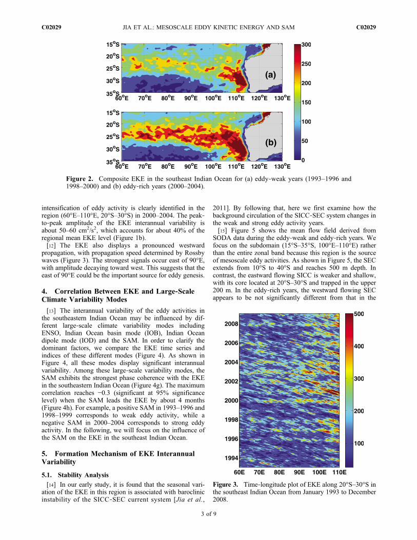
intensification of eddy activity is clearly identified in theregion (60°E–110°E, 20°S–30°S) in 2000–2004. The peak‐to‐peak amplitude of the EKE interannual variability isabout 50–60 cm2/s2, which accounts for about 40% of theregional mean EKE level (Figure 1b).[12] The EKE also displays a pronounced westward

propagation, with propagation speed determined by Rossbywaves (Figure 3). The strongest signals occur east of 90°E,with amplitude decaying toward west. This suggests that theeast of 90°E could be the important source for eddy genesis.

4. Correlation Between EKE and Large‐ScaleClimate Variability Modes

[13] The interannual variability of the eddy activities inthe southeastern Indian Ocean may be influenced by dif-ferent large‐scale climate variability modes includingENSO, Indian Ocean basin mode (IOB), Indian Oceandipole mode (IOD) and the SAM. In order to clarify thedominant factors, we compare the EKE time series andindices of these different modes (Figure 4). As shown inFigure 4, all these modes display significant interannualvariability. Among these large‐scale variability modes, theSAM exhibits the strongest phase coherence with the EKEin the southeastern Indian Ocean (Figure 4g). The maximumcorrelation reaches −0.3 (significant at 95% significancelevel) when the SAM leads the EKE by about 4 months(Figure 4h). For example, a positive SAM in 1993–1996 and1998–1999 corresponds to weak eddy activity, while anegative SAM in 2000–2004 corresponds to strong eddyactivity. In the following, we will focus on the influence ofthe SAM on the EKE in the southeast Indian Ocean.

5. Formation Mechanism of EKE InterannualVariability

5.1. Stability Analysis

[14] In our early study, it is found that the seasonal vari-ation of the EKE in this region is associated with baroclinicinstability of the SICC‐SEC current system [Jia et al.,

2011]. By following that, here we first examine how thebackground circulation of the SICC‐SEC system changes inthe weak and strong eddy activity years.[15] Figure 5 shows the mean flow field derived from

SODA data during the eddy‐weak and eddy‐rich years. Wefocus on the subdomain (15°S–35°S, 100°E–110°E) ratherthan the entire zonal band because this region is the sourceof mesoscale eddy activities. As shown in Figure 5, the SECextends from 10°S to 40°S and reaches 500 m depth. Incontrast, the eastward flowing SICC is weaker and shallow,with its core located at 20°S–30°S and trapped in the upper200 m. In the eddy‐rich years, the westward flowing SECappears to be not significantly different from that in the

Figure 2. Composite EKE in the southeast Indian Ocean for (a) eddy‐weak years (1993–1996 and1998–2000) and (b) eddy‐rich years (2000–2004).

Figure 3. Time‐longitude plot of EKE along 20°S–30°S inthe southeast Indian Ocean from January 1993 to December2008.

JIA ET AL.: MESOSCALE EDDY KINETIC ENERGY AND SAM C02029C02029

3 of 9

weak‐eddy years, but the eastward flowing SICC appears tobe stronger than that in the weak‐eddy years. The changes inthe velocity become clearer in Figure 6 where the verticalprofile of the zonal velocity is shown. The change of theSICC reaches about 0.7 cm/s, accounting for about 50% ofthe mean speed; while the change of the SEC is about0.1 cm/s, which only accounts for about 10% of the meanspeed. Here we define the vertical velocity shear as thezonal velocity difference between the upper (50 m) andlower (300 m) layers. So, the vertical velocity shear is

stronger in the eddy‐rich years (∼0.033 m/s) than in theeddy‐weak years (∼0.027 m/s).[16] In order to clarify how the interannual variation of

EKE relates to the vertical shear, both of them are displayedin Figure 7. The variations of the vertical velocity shearcorrelate well with the EKE with a lead of a few months(Figure 7a). This is confirmed in Figure 7b, which showsthat the maximum correlation between the two time seriesoccurs when the vertical shear leads the EKE by ∼5 months.[17] How does the change of the vertical shear associated

with the SICC‐SEC current system modify the EKE level?

Figure 4. Time series and correlation of the EKE in the southeast Indian Ocean and different climatevariability mode indices: (a, b) Nino3.4 index, (c, d) IOB index, (e, f) IOD index, and (g, h) SAM index.All indices are low‐pass filtered (>1 year), and the dashed lines indicate 95% significance level.

Figure 5. Latitude‐depth profile of temperature (solid contours, units °C) and zonal velocity (shading,units m s−1) along 100°E–110°E in the southeast Indian Ocean during (a) eddy‐weak years and (b) eddy‐rich years.

JIA ET AL.: MESOSCALE EDDY KINETIC ENERGY AND SAM C02029C02029

4 of 9

Following Qiu [1999], we adopt a 2.5‐layer reduced‐gravitymodel with two active upper layers and an infinitely deepabyssal layer to analyze the stability of the SICC‐SECcurrent system. This method was also used in analyzing theseasonal modulation of EKE in this region [Jia et al., 2011].The governing quasi‐geostrophic equation for the active twoupper layers can be expressed by

@

@tþ Un

@

@x

� �qn þ @Pn

@y

@�n

@x¼ 0 ð2Þ

where Un is the zonal geostrophic velocity, qn the pertur-bation potential vorticity, �n the perturbation stream func-tion, Pn the mean potential vorticity in the nth layer (n = 1

and 2). Assume that the mean flow Un is meridionallyuniform, qn and the meridional gradient of Pn can beexpressed by

qn ¼ r2�n þ �1ð Þn�2n

�1 � �2 � �n�2ð Þ ð3Þ

Pny ¼ � � �1ð Þn�2n

U1 � U2 � �nU2ð Þ ð4Þ

where gn =�n��1�3��2

is the stratification ratio, ln2 = �2��1ð ÞgHn

�0f 20is the

square of the internal Rossby radius in layer n, b = 2W cos80R

and f0 is the Coriolis parameter at the reference latitude 25°S.

Figure 6. Vertical profiles of zonal velocity averaged over the region (15°S–35°S, 100°E–110°E) ineddy‐weak (dotted line) and eddy‐rich (solid line) years.

Figure 7. (a) EKE (shaded areas) and vertical velocity shear (solid line). (b) Lagged correlation betweenEKE and vertical velocity shear shown in Figure 7a. The vertical velocity shear is defined as du = u(50 m) −u(300m) using the SODA product averaged in (15°S–35°S, 100°E–110°E). All time series are smoothed byapplying a 1 year low‐pass filter.

JIA ET AL.: MESOSCALE EDDY KINETIC ENERGY AND SAM C02029C02029

5 of 9

[18] Assume that equation (2) has a normal modesolution:

�n ¼ An cos kxþ ly� kctð Þ ð5Þ

substituting �n into equation (2) and a dispersion rela-tionship as well as the necessary and sufficient conditionfor instability in the 2.5‐layer model can be obtained:

c2 � U1 þ U2 � P þ Q

R

� �cþ U1U2 þP1yP2y

R� U1P

R� U2Q

R

� �¼ 0

ð6Þ

and

U1 � U2ð Þmin> �22� þ �2U2 ð7Þ

where P, Q and R are functions of k, l, d and l (see Qiu[1999] and Qiu and Chen [2004] for details). Equation (6)is the dispersion relationship for the complex wave speedc (c = cr + ici) from which we may detect the growth rate(kci) of the SICC‐SEC system and compare with theobserved results. The instability criterion equation (7)implies that once the condition (7) is satisfied, the sys-tem becomes baroclinically unstable. With the parametersappropriate for the southeast Indian Ocean (Table 1), this

requires U1 > l22b + (g2 + 1)U2max = −0.08 cm s−1. In

the SICC‐SEC system, the eastward flow SICC neverchanges directions, so the system is always baroclinicunstable.[19] With the parameters in Table 1, the dispersion rela-

tionship (equation (6)) is solved and the growth rates for theunstable waves are displayed in Figure 8. The system isunstable under both eddy‐weak and eddy‐rich conditions(ci ≠ 0) and the preferred wavelength scale of the mostunstable waves is ∼200 km, which corresponds well with theobserved mesoscale eddy propagation wavelength scale. Butthere are also many differences. The most unstable wave ineddy‐rich years has kci = 0.01 d−1, or an e‐folding time scaleof 100 days (Figure 8b), while the most unstable wave ineddy‐rich years is 0.007 d−1 or an e‐folding time scale of140 days (Figure 8a). In addition, the window for permis-sible unstable waves in eddy‐rich years is broader than thatin eddy‐weak years (Figure 8b versus Figure 8a). Therefore,the system in eddy‐rich years is baroclinically more unstablethan that in eddy‐weak years.[20] Notice that the major difference between the two is

the parameter U1 or the vertical velocity shear. In eddy‐richyears U1 is 0.0229 m s−1 and the vertical shear U1 − U2 is0.033 m s−1; well in eddy‐weak years U1 decreases to0.0174 m s−1 and U1 − U2 is 0.027 m s−1. The strongervertical velocity shear in eddy‐rich years work to intensifybaroclinic instability and result in enhanced mesoscale eddyactivities after the e‐folding time scale of the unstablewaves.[21] In summary, the 2.5‐layer reduced‐gravity model

results support the argument that the interannual variation inthe intensity of baroclinic instability of the SEC‐SICCcurrent system caused by the vertical shear modulates theeddy kinetic energy in the southeast Indian Ocean.

5.2. Modulation of the Vertical Velocity Shear by SAM

[22] According to the analysis above, the vertical velocityshear plays an important role in modulating the interannualchanges of EKE in the southeast Indian Ocean. In the fol-lowing, we will analyze how the SAM modulates the ver-tical velocity shear. The vertical velocity shear can be

Table 1. Parameter Values of the Region 15°S–35°S, 100°E–110°Ein Eddy‐Weak and Eddy‐Rich Yearsa

Parameter Eddy‐Weak Years Eddy‐Rich Years

f0 −6.16 × 10−5 s−1 −6.16 × 10−5 s−1

b 2.07 × 10−11 s−1 m−1 2.07 × 10−11 s−1 m−1

U1 0.0174 m s−1 0.0229 m s−1

U2 −0.01 m s−1 −0.01 m s−1

H1 150 m 150 mH2 300 m 300 mr1 24.40 s� 24.40 s�r2 26.71 s� 26.71 s�r3 27.80 s� 27.80 s�

aThe reference latitude for f0 and b is taken at 25°S; the other parametervalues are estimated from the SODA data.

Figure 8. Growth rate of unstable waves as a function of zonal and meridional wave number for(a) eddy‐weak years and (b) eddy‐rich years. Units for the growth rate are d−1. Parameters used in theanalysis are averaged in (15°S–35°S, 100°E–110°E).

JIA ET AL.: MESOSCALE EDDY KINETIC ENERGY AND SAM C02029C02029

6 of 9

related to the meridional temperature gradient through thethermal wind balance:

f@Ug

@z¼ �g

@T

@yð8Þ

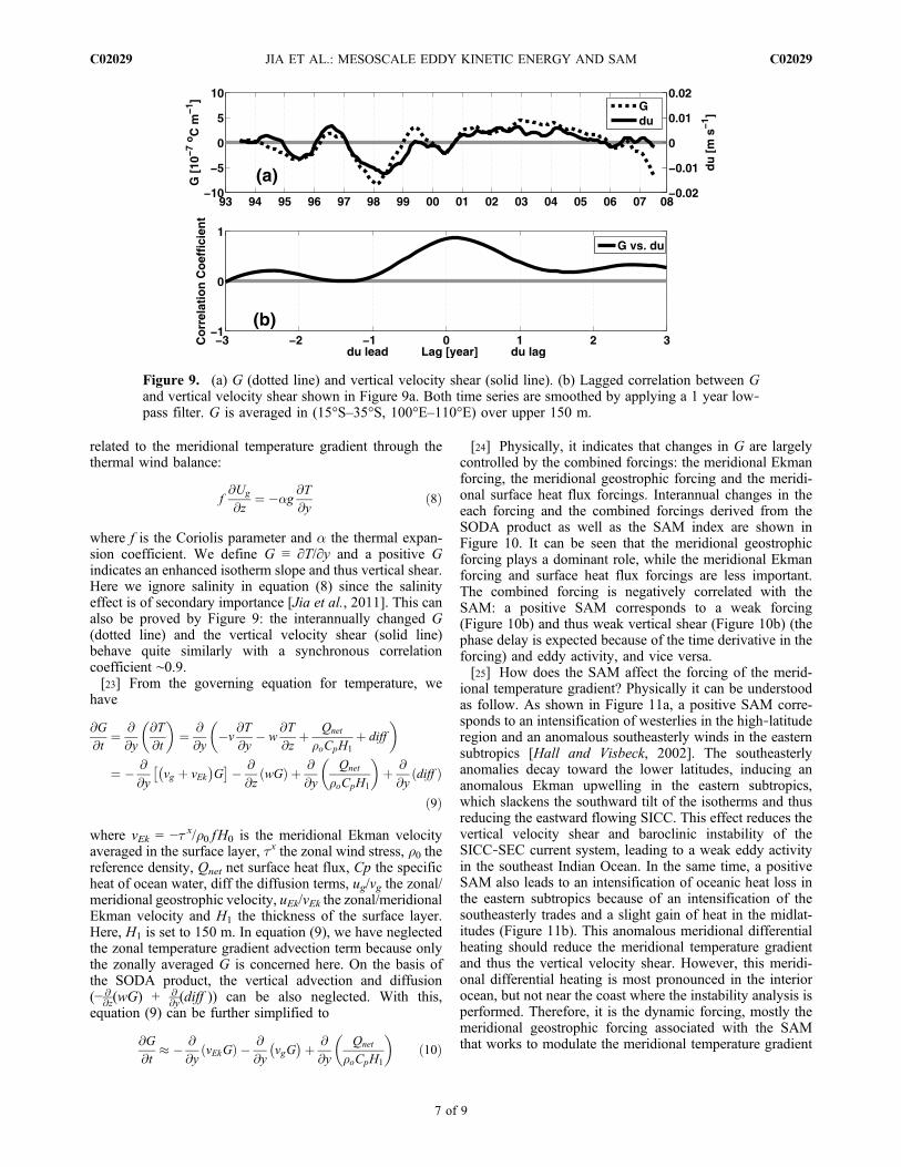
where f is the Coriolis parameter and a the thermal expan-sion coefficient. We define G ≡ ∂T/∂y and a positive Gindicates an enhanced isotherm slope and thus vertical shear.Here we ignore salinity in equation (8) since the salinityeffect is of secondary importance [Jia et al., 2011]. This canalso be proved by Figure 9: the interannually changed G(dotted line) and the vertical velocity shear (solid line)behave quite similarly with a synchronous correlationcoefficient ∼0.9.[23] From the governing equation for temperature, we

have

@G

@t¼ @

@y

@T

@t

� �¼ @

@y�v

@T

@y� w

@T

@zþ Qnet

�oCpH1þ diff

� �

¼ � @

@yvg þ vEk� �

G� �� @

@zwGð Þ þ @

@y

Qnet

�oCpH1

� �þ @

@ydiffð Þ

ð9Þ

where vEk = −t x/r0 fH0 is the meridional Ekman velocityaveraged in the surface layer, tx the zonal wind stress, r0 thereference density, Qnet net surface heat flux, Cp the specificheat of ocean water, diff the diffusion terms, ug/vg the zonal/meridional geostrophic velocity, uEk/vEk the zonal/meridionalEkman velocity and H1 the thickness of the surface layer.Here, H1 is set to 150 m. In equation (9), we have neglectedthe zonal temperature gradient advection term because onlythe zonally averaged G is concerned here. On the basis ofthe SODA product, the vertical advection and diffusion(− @

@z(wG) + @@y(diff )) can be also neglected. With this,

equation (9) can be further simplified to

@G

@t� � @

@yvEkGð Þ � @

@yvgG� �þ @

@y

Qnet

�oCpH1

� �ð10Þ

[24] Physically, it indicates that changes in G are largelycontrolled by the combined forcings: the meridional Ekmanforcing, the meridional geostrophic forcing and the meridi-onal surface heat flux forcings. Interannual changes in theeach forcing and the combined forcings derived from theSODA product as well as the SAM index are shown inFigure 10. It can be seen that the meridional geostrophicforcing plays a dominant role, while the meridional Ekmanforcing and surface heat flux forcings are less important.The combined forcing is negatively correlated with theSAM: a positive SAM corresponds to a weak forcing(Figure 10b) and thus weak vertical shear (Figure 10b) (thephase delay is expected because of the time derivative in theforcing) and eddy activity, and vice versa.[25] How does the SAM affect the forcing of the merid-

ional temperature gradient? Physically it can be understoodas follow. As shown in Figure 11a, a positive SAM corre-sponds to an intensification of westerlies in the high‐latituderegion and an anomalous southeasterly winds in the easternsubtropics [Hall and Visbeck, 2002]. The southeasterlyanomalies decay toward the lower latitudes, inducing ananomalous Ekman upwelling in the eastern subtropics,which slackens the southward tilt of the isotherms and thusreducing the eastward flowing SICC. This effect reduces thevertical velocity shear and baroclinic instability of theSICC‐SEC current system, leading to a weak eddy activityin the southeast Indian Ocean. In the same time, a positiveSAM also leads to an intensification of oceanic heat loss inthe eastern subtropics because of an intensification of thesoutheasterly trades and a slight gain of heat in the midlat-itudes (Figure 11b). This anomalous meridional differentialheating should reduce the meridional temperature gradientand thus the vertical velocity shear. However, this meridi-onal differential heating is most pronounced in the interiorocean, but not near the coast where the instability analysis isperformed. Therefore, it is the dynamic forcing, mostly themeridional geostrophic forcing associated with the SAMthat works to modulate the meridional temperature gradient

Figure 9. (a) G (dotted line) and vertical velocity shear (solid line). (b) Lagged correlation between Gand vertical velocity shear shown in Figure 9a. Both time series are smoothed by applying a 1 year low‐pass filter. G is averaged in (15°S–35°S, 100°E–110°E) over upper 150 m.

JIA ET AL.: MESOSCALE EDDY KINETIC ENERGY AND SAM C02029C02029

7 of 9

and thus the vertical velocity shear and the baroclinicinstability of the SICC‐SEC system.

6. Summary and Discussions

[26] In this paper, interannual modulation of mesoscaleeddy activities in the southeast Indian Ocean along ∼25°S isinvestigated on the basis of the 16 year satellite altimetryobservations. It is found that the dynamic forcing associatedwith the SAM can modulate the baroclinic instability of theSICC‐SEC current system, leading to changes of the EKE inthe southeast Indian Ocean.[27] Here, we emphasize the role of the SAM in the

interannual modulation of the EKE in the southeast IndianOcean, but do not exclude other impacts. Mesoscale eddyactivities here can also be affected by other processes

because of a unique circulation system in this region,including the Leeuwin Current (LC). Studies have indicatedthat the LC variability also has a well‐defined seasonal andinterannual cycle [e.g., Feng et al., 2003;Morrow and Birol,1998; Peter et al., 2005]. Feng et al. [2003] studied theENSO related interannual variations of the Leeuwin Currentat 32°S in this region and found the Leeuwin Current isstronger during a La Niña year and weaker during anEl Niño year. Eddies and baroclinic Rossby waves are foundto be generated by the LC variations and then propagate tothe west [e.g., Rennie et al., 2007; Morrow et al., 2003;Birol and Morrow, 2001, 2003]. This appears to be sup-ported by the correlation between the EKE in the southeastIndian Ocean and the Nino3.4 index, which shows a sig-nificant correlation when the Nino3.4 leads the EKE by

Figure 11. Synchronous correlation between the Southern Annular Mode index and (a) the wind stress(arrows) and Ekman pumping (shaded) and (b) net surface heat flux (positive downward). The data arelow‐pass filtered by applying a 1 year low‐pass filter.

Figure 10. Time series of (a) meridional Ekman forcing term (dotted line), geostrophic forcing term(solid line), heat flux forcing term (dash‐dotted line), and the SAM index (shaded areas) and (b) combinedforcing (shaded bars), the vertical velocity shear (solid line), and the SAM index (dotted line). The forcingis averaged in (15°S–35°S, 100°E–110°E) over upper 150 m.

JIA ET AL.: MESOSCALE EDDY KINETIC ENERGY AND SAM C02029C02029

8 of 9

about 1 year (Figure 4b). Future studies are needed toquantify the effects of the eastern boundary processes inmesoscale processes in the interior ocean.

[28] Acknowledgments. This work is supported by China NationalNatural Science Foundation Projects (40788002, 40876001), China ForeignExpert “111” project through the Ministry of Education, and NSFCCreative Research Group Project (40921004). We are also very gratefulto the two anonymous reviewers for their constructive comments.

ReferencesBirol, F., and R.Morrow (2001), Source of the baroclinic waves in the south-east Indian Ocean, J. Geophys. Res., 106, 9145–9160, doi:10.1029/2000JC900044.

Birol, F., and R. Morrow (2003), Separation of the quasi‐semiannualRossby waves from the eastern boundary of the Indian Ocean,J. Mar. Res., 61, 707–723, doi:10.1357/002224003322981110.

Carton, J. A., G. Chepurin, X. Cao, and B. Giese (2000), A simple oceandata assimilation analysis of the global upper ocean 1950–95. Part I:Methodology, J. Phys. Oceanogr., 30, 294–309, doi:10.1175/1520-0485(2000)030<0294:ASODAA>2.0.CO;2.

Eden, C., and C. Böning (2002), Sources of eddy kinetic energy in the Lab-rador Sea, J. Phys. Oceanogr., 32, 3346–3363, doi:10.1175/1520-0485(2002)032<3346:SOEKEI>2.0.CO;2.

Feng, M., G. Meyers, A. Pearce, and S. Wijffels (2003), Annual andinterannual variations of the Leeuwin Current at 32°S, J. Geophys.Res., 108(C11), 3355, doi:10.1029/2002JC001763.

Hall, A., and M. Visbeck (2002), Synchronous variability in the SouthernHemisphere atmosphere, sea ice, and ocean resulting from the annularmode, J. Clim., 15, 3043–3057, doi:10.1175/1520-0442(2002)015<3043:SVITSH>2.0.CO;2.

Jia, F., L. Wu, and B. Qiu (2011), Seasonal modulation of eddy kineticenergy and its formation mechanism in the southeast Indian Ocean,J. Phys. Oceanogr., in press.

Ma, H., and L. Wu (2011), Global teleconnections in response to fresheningover the Antarctic Ocean, J. Clim., doi:10.1175/2010JCLI3634.1, in press.

Marshall, G. J. (2003), Trends in the Southern Annular Mode from obser-vations and reanalyses, J. Clim., 16, 4134–4143, doi:10.1175/1520-0442(2003)016<4134:TITSAM>2.0.CO;2.

Marshall, G. J., A. Orr, N. P. M. van Lipzig, and J. C. King (2006), Theimpact of a changing Southern Hemisphere Annular Mode on AntarcticPeninsula summer temperatures, J. Clim., 19, 5388–5404, doi:10.1175/JCLI3844.1.

Mo, K. C. (2000), Relationships between low‐frequency variability in theSouthern Hemisphere and sea surface temperature anomalies, J. Clim.,13, 3599–3610, doi:10.1175/1520-0442(2000)013<3599:RBLFVI>2.0.CO;2.

Morrow, R., and F. Birol (1998), Variability in the southeast Indian Oceanfrom altimetry: Forcing mechanisms for the Leeuwin Current, J. Geophys.Res., 103, 18,529–18,544, doi:10.1029/98JC00783.

Morrow, R., F. Fang, M. Fieux, and R. Molcard (2003), Anatomy of threewarm‐core Leeuwin Current eddies, Deep Sea Res., 50, 2229–2243,doi:10.1016/S0967-0645(03)00054-7.

Palastanga, V., P. J. van Leeuwen, M. W. Schouten, and W. P. M. de Ruijter(2007), Flow structure and variability in the subtropical Indian Ocean:Instability of the South Indian Ocean Countercurrent, J. Geophys. Res.,112, C01001, doi:10.1029/2005JC003395.

Penduff, T., B. Barnier, W. K. Dewar, and J. J. O’Brien (2004), Dynamicalresponse of the oceanic eddy field to the North Atlantic Oscillation: A

model‐data comparison, J. Phys. Oceanogr. , 34 , 2615–2629,doi:10.1175/JPO2618.1.

Peter, B. N., P. Sreeraj, and K. G. Vimal Kumar (2005), Structure andvariability of the Leeuwin Current in the south eastern Indian Ocean,J. Indian Geophys. Union, 9(2), 107–119.

Qiu, B. (1999), Seasonal eddy modulation of the North Pacific SubtropicalCountercurrent: TOPEX/Poseidon observations and theory, J. Phys.Oceanogr., 29, 2471–2486, doi:10.1175/1520-0485(1999)029<2471:SEFMOT>2.0.CO;2.

Qiu, B., and S. Chen (2004), Seasonal modulations in the eddy field of theSouth Pacific Ocean, J. Phys. Oceanogr., 34, 1515–1527, doi:10.1175/1520-0485(2004)034<1515:SMITEF>2.0.CO;2.

Qiu, B., and S. Chen (2010a), Interannual variability of the North PacificSubtropical Countercurrent and its associated mesoscale eddy field,J. Phys. Oceanogr., 40, 213–225, doi:10.1175/2009JPO4285.1.

Qiu, B., and S. Chen (2010b), Eddy‐mean flow interaction in the decadallymodulating Kuroshio Extension system, Deep Sea Res., Part II, 57,1097–1110, doi:10.1016/j.dsr2.2008.11.036.

Rao, S. A., and S. K. Behera (2005), Subsurface influence on SST in thetropical Indian ocean: Structure and interannual variability, Dyn. Atmos.Oceans, 39, 103–135, doi:10.1016/j.dynatmoce.2004.10.014.

Rayner, N. A., D. E. Parker, E. B. Horton, C. K. Folland, L. V. Alexander,D. P. Rowell, E. C. Kent, and A. Kaplan (2003), Global analyses of seasurface temperature, sea ice, and night marine air temperature since thelate nineteenth century, J. Geophys. Res. , 108(D14), 4407,doi:10.1029/2002JD002670.

Rennie, S. J., C. B. Pattiaratchi, and R. D. McCauley (2007), Eddy forma-tion through the interaction between the Leeuwin Current, LeeuwinUndercurrent and topography, Deep Sea Res., Part II, 54, 818–836,doi:10.1016/j.dsr2.2007.02.005.

Saji, N. H., B. N. Goswami, P. N. Vinayachandran, and T. Yamagata(1999), A dipole in the tropical Indian Ocean, Nature, 401, 360–363,doi:10.1038/43854.

Schott, F. A., S.‐P. Xie, and J. P. McCreary Jr. (2009), Indian Ocean cir-culation and climate variability, Rev. Geophys., 47 , RG1002,doi:10.1029/2007RG000245.

Siedler, G., M. Rouault, and J. R. E. Lutjeharms (2006), Structure andorigin of the subtropical South Indian Ocean Countercurrent, Geophys.Res. Lett., 33, L24609, doi:10.1029/2006GL027399.

Silvestri, G., and C. Vera (2009), Nonstationary impacts of the SouthernAnnular Mode on Southern Hemisphere climate, J. Clim., 22,6142–6148, doi:10.1175/2009JCLI3036.1.

Thompson, D. W. J., and J. M. Wallace (2000), Annular modes in theextratropical circulation, part I: Month‐to‐month variability, J. Clim.,13, 1000–1016, doi:10.1175/1520-0442(2000)013<1000:AMITEC>2.0.CO;2.

Webster, P. J., A. M. Moore, J. P. Loschnigg, and R. R. Leben (1999),Coupled oceanic‐atmospheric dynamics in the Indian Ocean during1997–98, Nature, 401, 356–360, doi:10.1038/43848.

Xie, S.‐P., H. Annamali, and F. Schott (2002), Structure and mechanismsof south Indian Ocean climate variability, J. Clim., 15, 864–878,doi:10.1175/1520-0442(2002)015<0864:SAMOSI>2.0.CO;2.

Yang, J., Q. Liu, S.‐P. Xie, Z. Liu, and L. Wu (2007), Impact of the IndianOcean SST basin mode on the Asian summer monsoon, Geophys. Res.Lett., 34, L02708, doi:10.1029/2006GL028571.

F. Jia, J. Lan, and L. Wu, Physical Oceanography Laboratory, OceanUniversity of China, 238 Songling Rd., Qingdao 266100, China.(afanayang31@163.com)B. Qiu, Department of Oceanography, University of Hawai’i at Mānoa,

100 Pope Rd., Honolulu, HI 96822, USA.

JIA ET AL.: MESOSCALE EDDY KINETIC ENERGY AND SAM C02029C02029

9 of 9