interactive discovery of coordinated relationship chains...

39

Interactive Discovery of Coordinated Relationship Chainswith Maximum Entropy Models

HAO WU*, Virginia Tech

MAOYUAN SUN*, University of Massachusetts Dartmouth

PENG MI, Virginia Tech

NIKOLAJ TATTI, Aalto University

CHRIS NORTH, Virginia Tech

NAREN RAMAKRISHNAN, Virginia Tech

Modern visual analytic tools promote human-in-the-loop analysis but are limited in their abilityto direct the user toward interesting and promising directions of study. This problem is especiallyacute when the analysis task is exploratory in nature, e.g., the discovery of potentially coordinatedrelationships in massive text datasets. Such tasks are very common in domains like intelligenceanalysis and security forensics where the goal is to uncover surprising coalitions bridging multipletypes of relations. We introduce new maximum entropy models to discover surprising chains ofrelationships leveraging count data about entity occurrences in documents. These models areembedded in a visual analytic system called MERCER that treats relationship bundles as first classobjects and directs the user toward promising lines of inquiry. We demonstrate how user inputcan judiciously direct analysis toward valid conclusions whereas a purely algorithmic approachcould be led astray. Experimental results on both synthetic and real datasets from the intelligencecommunity are presented.

CCS Concepts: •Mathematics of computing→Exploratory data analysis; •Human-centeredcomputing →Visual analytics; •Computing methodologies →Maximum entropy mod-eling; •Information systems →Data mining;

Additional Key Words and Phrases: Maximum entropy models, multi-relational pattern mining,

interactive visual data exploration

ACM Reference format:Hao Wu*, Maoyuan Sun*, Peng Mi, Nikolaj Tatti, Chris North, and Naren Ramakrishnan. 2010.Interactive Discovery of Coordinated Relationship Chains with Maximum Entropy Models. ACMTrans. Knowl. Discov. Data. 9, 4, Article 39 (March 2010), 36 pages.DOI: 0000001.0000001

*These authors contributed equally to this work.

Author’s addresses: H. Wu and N. Ramakrishnan, Discovery Analytics Center, Virginia Tech, Arlington,

VA, USA; M. Sun, Computer and Information Science, University of Massachusetts Dartmouth, Dartmouth,MA, USA; P. Mi, VMWare Inc., Palo Alto, CA, USA; N. Tatti, Department of Information and Computer

Science, Aalto University School of Science, Aalto, Finland; C. North, Discovery Analytics Center, VirginiaTech, Blacksburg, VA, USA.Permission to make digital or hard copies of all or part of this work for personal or classroom use is granted

without fee provided that copies are not made or distributed for profit or commercial advantage and that

copies bear this notice and the full citation on the first page. Copyrights for components of this workowned by others than ACM must be honored. Abstracting with credit is permitted. To copy otherwise,

or republish, to post on servers or to redistribute to lists, requires prior specific permission and/or a fee.Request permissions from [email protected].

© 2010 ACM. 1556-4681/2010/3-ART39 $15.00

DOI: 0000001.0000001

ACM Transactions on Knowledge Discovery from Data, Vol. 9, No. 4, Article 39. Publication date:

March 2010.

39:2 H. Wu et al.

1 INTRODUCTION

Unstructured exploration of relationships from large text datasets is a crucial problemin many application domains, for example, intelligence analysis, biomedical discovery,analysis of legal briefs and opinions. The state-of-the-art today involves two broad classesof techniques. Visual analytic tools, for example Jigsaw [47], support the exploration ofrelationships extracted from large text datasets. While they promote human-in-the-loopanalysis, identifying promising leads to explore is left to the creativity of the user. At theother end of the spectrum, text relationship exploration techniques such as storytelling [21]provide interesting artifacts (for example, stories, summaries) for analysis but are limited intheir ability to incorporate user input to steer the discovery process.

Our goal here is to realize an amalgamation of algorithmic and human-driven techniquesto support the discovery of coordinated relationship chains from document collections. Acoordinated relationship (also called a bicluster) is one in which a group of entities arerelated to another group of entities via a common relation. It is thus a generalization ofa relationship instance. A chain of such coordinated relationships enables us to bundlegroups of entities across various domains and relate them through a succession of individualrelationships. The primary artifact of interest are thus chains summarizing how entities in adocument collection are related. We introduce new maximum entropy (MaxEnt) models toidentify surprising chains of interest and rank them for inspection by the user. In intelligenceanalysis, such chains can reveal how hitherto unconnected people or places are relatedthrough a sequence of intermediaries. In biomedical discovery, such chains can reveal howproteins involved in distinct pathways are related through cross-talk via other proteins orsignaling molecules. In legal briefs, one can use chains to determine how rationale for courtopinions vary over the years and are buttressed by the precedence structure implicit in legalhistory.

As shown in Fig. 1 (left), we propose an interactive approach wherein user feedback iswoven at each stage and used to rank the most interesting chains for further exploration.Such user feedbacks are also taken into account by the algorithm for further investigationsof the data. We will demonstrate through case studies how such an approach gets usersto their intended objectives compared to a purely algorithmic approach (Fig. 1 (right)).The work presented here is implemented in a system – Maximum Entropy Relational ChainExploRer (MERCER) that uses a variety of visual exploration strategies and algorithmicmeans to foster user exploration.

Our key contributions are:

(1) MERCER is a marriage of two of our prior works [51, 61] but supercedes the state-of-the-art in these papers in significant, orthogonal, ways. MERCER is a significantimprovement over the work presented by Sun et al. [51] because the authors providesupport for only manual exploration of coordinated relationships. MERCER is alsoa significant improvement over the work presented by Wu et al. [61] because thiswork only presents approaches to rank chains involving a binary maximum entropymodel whereas MERCER introduces more general maximum entropy approachesfor real-valued data.

(2) We present two path strategies (full path and stepwise) to help analyze datasets.Using our proposed maximum entropy models, the full path strategy discovers themost surprising bicluster chains from all possible chains involving an analyst-selectedbicluster. The stepwise strategy evaluates biclusters neighboring a user-specifiedone, and prioritizes possible connected information with the current pieces under


March 2010.

Interactive Discovery of Coordinated Relational Chains 39:3

Fig. 1. Illustration of MERCER. (left) Discovery of coordinated relationship chains is aided by regularincorporation of user feedback. (right) Unaided algorithmic discovery of relationship chains leads to longlists of patterns that might not lead to the desired answer.

investigation. Both strategies directs analysts to reveal hidden plots involvingsurprising relational patterns.

(3) We describe new visual encodings and summary as well as detailed views to supportuser-guided exploration of coordinated relationships in massive datasets. Besidesbasic color codings (for example, connection-oriented highlighting [51]), MERCERoffers highlighting mechanisms aimed at pointing out surprising information. En-hanced with the proposed maximum entropy models, this highlighting capabilitynot only directs user’s attention to important connected pieces of information, butalso visually prioritizes them in a usable manner.

(4) We describe experimental results on both large, synthetic datasets (to illustrateefficiency and effectiveness of our algorithms) and small, real datasets (to illustratehow users can interactively explore a realistic text dataset). In particular, we showhow MERCER enables the user to more quickly arrive at plots of interest than thetraditional manual approach described in our previous work [51].


March 2010.

39:4 H. Wu et al.

……

………………

…………

……

……

……

……

……

……Do

cs

𝑈" 𝑈#… 𝑈$ …Doc-EntityMatrix

……

……

……

……

……

…

……

……

……

……

……

………

……

……

……

……

…

Entity-EntityRelations(Sec.4)

𝑈 "

𝑈%

𝑈 $

𝑈& 𝑈#

𝑈 ' ……

MaxEntModel(Sec.3)

Biclusters

Background

Inform

ation

Visualization(Sec.5)

Visualize

AnalystInteractions

Feedback

…

………

Chains Plots

&

Fig. 2. MERCER system workflow.

2 PRELIMINARIES

Figure 2 illustrates the workflow in MERCER. By taking the background information fromthe document-entity transactional matrix, the MERCER system infers the maximum entropymodel, which will be described in detail in Section 3. From the document-entity matrix,multiple entity-entity relations are extracted and surprisingness measure for relationalpatterns is defined based on the MaxEnt model (Section 4). By interacting with analysts,our visualization interface displays the surprising relational patterns discovered from themultiple entity-entity relations, and also provides analysts’ feedback to the MaxEnt model,which will in turn help to further discover additional surprising patterns (Section 5). Inthis section, we introduce some preliminary concepts and notations that will be useful tounderstand the MERCER system and the rest of this paper.


March 2010.


Multi-relational schema. Suppose that we have l domains or universes which will bedenoted by Ui, where i = 1, 2, . . . , l, throughout the paper. An entity is a member of Ui andan entity set is just a subset of Ui. We use R = R(Ui, Uj) to represent a binary relationbetween some domains Ui and Uj . Given a set of domains U = {U1, U2, . . . , Ul} and aset of relations R = {R1, R2, . . . , Rm}, a multi-relational schema S(U ,R) is defined as aconnected bipartite graph whose vertex set is given by U ∪R and edge set is the collectionof edges each of which connects a relation Rj ∈ R and a domain Ui ∈ U that the relationRj involves. In this paper, we will focus on binary relationships, e.g. each Rj is a binaryrelation. Thus, all the vertices in R in the bipartite graph will have degree of two. Binaryrelations usually can be represented as binary data matrices. In the rest of this paper, wewill use these two terms interchangeably depending on which one is easier to use to presentand explain our proposed model and algorithm.

Tiles. A tile [14] T is essentially a rectangle in a binary data matrix. Formally, it isdefined as a tuple T = (r(T ), c(T )) where r(T ) is a set of row identifiers (e.g., row IDs)and c(T ) is a set of column identifiers (e.g., column IDs) over the data matrix. This mostgeneral form definition imposes no constraints on values of the matrix entries identified by atile. Thus, each element in a tile can be any valid value in the data matrix. In the binarycase, when all entries within a tile T have the same value (i.e., either all 1s or all 0s), T isan exact tile. Otherwise we say it is a noisy tile.

Biclusters. As local patterns of interest over binary relations, we consider binary biclusters.Although the concept of biclusters was first introduced over real-valued data [5], as ageneralization of this concept to binary data, we will use the word biclusters to refer tothe local patterns over binary relations defined below in the rest of this paper. A bicluster,represented by B = (Ei, Ej), on a relation R = R(Ui, Uj), consists of two entity sets Ei ⊆ Uiand Ej ⊆ Uj such that Ei × Ej ⊆ R. As such a bicluster is a special case of an exact tile,one in which all the elements are 1. Further, we say a bicluster B = (Ei, Ej) is closed if forevery entity ei ∈ Ui \ Ei, there is some entity ej ∈ Ej such that (ei, ej) /∈ R and for everyentity ej ∈ Uj \Ej , there is some entity ei ∈ Ei such that (ei, ej) /∈ R. In other words, Eiis maximal (w.r.t. Ej) so that we cannot add more elements to Ei without violating thepremise of a bicluster. If a pair of entities ei ∈ Ui, ej ∈ Uj belongs to a bicluster B, werepresent this fact by (ei, ej) ∈ B. In the rest of this paper, all the biclusters we mentionrefer to closed biclusters.

Redescriptions. Suppose that we have two biclusters B = (Ei, Ej) and C = (Fj , Fk),where Ei ⊆ Ui, Ej , Fj ⊆ Uj , and Fk ⊆ Uk. Note that Ej and Fj lie in the same domain.Assume that we are given a threshold 0 ≤ ϕ ≤ 1. We define that B and C are approximateredescriptors of each other, which we represent by B ∼ϕ,j C if the Jaccard coefficient|Ej ∩ Fj | / |Ej ∪ Fj | ≥ ϕ. The threshold ϕ is usually specified by users, consequently weoften drop ϕ from the notation and write B ∼j C. The index j indicates the commondomain over which we should take the Jaccard coefficient. When this domain is clear fromthe context we often ignore the index j from the notation. If B ∼1,j C, then we must haveEj = Fj in which case we say that B is an exact redescription of C. This definition coincideswith the definition given by Zaki and Ramakrishnan [64], who define redescriptions foritemsets over their mutual domain, transactions, such that the set Ej consists of transactionscontaining itemset Ei and the set Fj consists of transactions containing itemset Fk.


March 2010.

39:6 H. Wu et al.

Bicluster Chains. We define a bicluster chain C as an ordered set of biclusters {B1, B2, . . . , Bk}and an ordered bag of domain indices {j1, j2, . . . , jk−1} such that for each pair of adjacentbiclusters they are redescriptions of each other, e.g. Bi ∼ji Bi+1. Note that this definitionimplicitly requires that two adjacent biclusters share a common domain. If a bicluster BRi

is a member of a bicluster chain C, we will denote this by BRi ∈ C in this paper.

Surprisingness. In the knowledge discovery tasks studied here, the primary goal is toextract novel, interesting, or unusual knowledge. That is, we aim to discover results thatare highly informative compared to what we already know—we are not so much interestedin what we already do know, or what can be trivially induced from such knowledge. To thisend, we suppose a probability distribution p that represents the user’s current beliefs aboutthe data. When mining the data (e.g., for a bicluster or chain), we can use p to determinethe likelihood of a result under our current beliefs: if the likelihood is high, this indicatesthat we probably already know about it, and thus, reporting it to users would provide littlenew information. In contrast, if the likelihood of a result is very low, the result would bequite interesting, thus potentially conveying a lot of new information. In Section 3, we willdiscuss how to infer such a probability distribution for both binary and real-valued datamatrices.

Problem Statement. Given a multi-relational dataset, a bicluster chain across multiplerelations describes a progression of entity coalitions. We are particularly interested inchains that are surprising w.r.t. what we already know since these could help to uncoverthe plots hidden in the multi-relational dataset. More formally, given a multi-relationaldataset schema S(U ,R), where U = {U1, U2, . . . , Ul} and R = {R1, R2, . . . , Rm}, we aim toiteratively discover non-redundant bicluster chains that are most surprising with respectto each other and w.r.t. the background knowledge with the assistance of visual analysistechniques.

3 TILE-BASED MAXIMUM ENTROPY MODEL

Our problem statement is based on a notion of a multi-relational schema. In practice, oneapproach to infer such multi-relational datasets from a transactional dataset is to rely onthe item co-occurrence information in transactions where these items involved in binaryrelations are from different domains (e.g., entities discovered from a document collection,and then subsequently related by co-occurrence). More specifically, we assume that ourschema was generated from a transactional data matrix D (see Fig. 2). This data matrixcan be viewed as a matrix of size N -by-M . We will introduce the method of obtaining aschema from D in Section 4. In this approach the columns of D correspond to the entitiesof the schema. Hence, we will refer to the columns of D as entities.

3.1 Maximum Entropy Model for Binary Data

In this section, we will formally define the maximum entropy (MaxEnt) model for binarydata matrices using tiles as background knowledge—recall that a tile is a more generalnotion than a bicluster. In order to understand the model derivation in the context of binarydata, we first introduce some notations for binary MaxEnt model. Then, MaxEnt theory formodeling binary data given tiles as background information will be reviewed, and finally, wewill identify how we can estimate the model by maximizing the likelihood.


March 2010.


3.1.1 Notation for Tiles. Suppose we are given a binary data matrix D of size N -by-Mand a tile T , we define the (relative) frequency of T in D, fr(T ;D), as

fr(T ;D) =1

|σ(T )|∑

(i,j)∈σ(T )

D(i, j) . (1)

Here, D(i, j) denotes the entry (i, j) in D, and σ(T ) = {(i, j) | i ∈ r(T ), j ∈ c(T )} representsthe cells covered by tile T in the data matrix D. Remember that a tile T is called ‘exact’ ifthe corresponding entries D(i, j) are all 1 (resp. 0) for all (i, j) ∈ σ(T ). This indicates forexact tiles, fr(T ;D) = 1 or fr(T ;D) = 0. Otherwise, it is called a ‘noisy’ tile.

Let D be the space of all the possible binary data matrices of size N -by-M , and p be theprobability distribution defined over the data matrix space D. Then, the expected frequencyof the tile T with respect to the data matrix probability distribution p is defined as

fr(T ; p) = E [fr(T ;D)] =∑D∈D

p(D)fr(T ;D). (2)

By combining these definitions, we can derive the following lemma.

Lemma 3.1 ([61]). Given a dataset distribution p and a tile T , the expected frequency oftile T is

fr(T ; p) =1

|σ(T )|∑

(i,j)∈σ(T )

p ((i, j) = 1) ,

where p((i, j) = 1) represents the probability of a data matrix having 1 at entry (i, j) underthe data matrix distribution p.

Lemma 3.1 can be trivially proved by substituting fr(T ;D) in Equation (2) with Equa-tion (1) and switching the summations.

3.1.2 Global MaxEnt Model from Tiles. Suppose we are given a set of tiles T , and each tileT ∈ T is associated with a frequency γT—which typically can be trivially calculated fromthe data. This tile set T provides information about the data at hand, and we would like toestimate a distribution p over the space of all the possible data matrices D which conformwith the information given in T . In other words, we would like to be able to determine howprobable is a data matrix D ∈ D given the tile set T .

To derive a good statistical model, we adopt a principled approach and apply the maximumentropy principle [23] from information theory. Generally speaking, the MaxEnt principleidentifies the best distribution given background knowledge as the unique distributionwhich represents the provided background information but is maximally random otherwise.MaxEnt modeling has recently attracted much attention in the realm of data miningas a tool for identifying subjective interestingness of results with respect to backgroundknowledge [10, 29, 55, 60].

To formally define a MaxEnt distribution, we first specify the space of probability dis-tribution candidates. Here, these are all the possible data matrix distributions which areconsistent with the information given by the tile set T . Hence, we define the data matrix dis-tribution space as: P = {p | fr(T ; p) = γT ,∀T ∈ T }. Among all these possible distributioncandidates, we choose the distribution p∗T that maximizes the entropy,

p∗T = arg maxp∈P

H(p) .


March 2010.

39:8 H. Wu et al.

Here, H(p) denotes the entropy of the data matrix probability distribution p, which isdefined as

H(p) = −∑D∈D

p(D) log p(D) .

Next, to infer the MaxEnt distribution p∗T , we rely on a classical theorem about how MaxEntdistributions can be factorized. In particular, Theorem 3.1 proved by Csiszar [6] states thatfor a given set of testable statistics T (background knowledge, here a tile set), a distributionp∗T is the maximum entropy distribution if and only if it can be written as

p∗T (D) ∝

{exp

( ∑T∈T

λT · |σ(T )| · fr(T ;D))

D 6∈ Z

0 D ∈ Z ,

where λT is the weight for fr(T ;D) and Z is a collection of data matrices such that p(D) = 0,for all p ∈ P.

De Bie [10] formalized the MaxEnt model for a binary matrix D given row and columnmargins—also known as a Rasch [37] model. Here, we consider a more general scenario ofbinary data and tiles. In this case, we additionally know [Theorem 2 in 29, 55] that given atile set T , with T (i, j) = {T ∈ T | (i, j) ∈ σ(T )}, we can further factorize the maximumentropy distribution p∗T as

p∗T =∏

(i,j)∈D

p∗T ((i, j) = D(i, j)) ,

where

p∗T ((i, j) = 1) =exp

(∑T∈T (i,j) λT

)exp

(∑T∈T (i,j) λT

)+ 1

or 0, 1 .

This result allows us to represent the MaxEnt distribution p∗T of binary data matrices givenbackground information in the form of a set of tiles T by a product of Bernoulli randomvariables, each of which denotes a single entry in the data matrix D. We need to emphasizehere that this model is a different MaxEnt model compared to that when independencebetween rows in the data matrix D is assumed [see, e.g., 35, 54, 60]. Here, for example,in the special case where the given tiles are all exact (γT = 0 or 1), the resulting MaxEntdistribution will have a very simple form:

p∗T ((i, j) = 1) =

{γT if ∃T ∈ T such that (i, j) ∈ σ(T )12 otherwise.

3.1.3 Inferring the MaxEnt Distribution. To estimate the parameters of the Bernoullirandom variables mentioned above, we follow a standard approach and apply the well knownIterative Scaling (IS) algorithm [7] to infer the tile based MaxEnt model over binary datamatrices. Algorithm 1 illustrates the details of this IS algorithm for binary data. Brieflyspeaking, for each tile T ∈ T , the algorithm updates the probability distribution p suchthat the expected frequency of 1s under the distribution p matches the given frequency γT .Clearly, during this iterative update procedure, we may change the expected frequenciesof other tiles, and hence several iterations are required until the probability distribution pconverges. For the proof of convergence, please refer to Theorem 3.2 proved by Csiszar [6].In practice, the algorithm typically takes on the order of seconds to converge.


March 2010.


ALGORITHM 1: Iterative Scaling Algorithm (binary dataset)

input : a tile set T , target frequencies {γT | T ∈ T }.output : maximum entropy distribution p∗T ← p.

1 p← a N -by-M matrix with all values of 12;

2 for T ∈ T , γT = 0, 1 do3 p(i, j)← γT , for all (i, j) ∈ σ(T );

4 end

5 while not converged do6 for T ∈ T , 0 < γT < 1 do

7 find x such that: fr(T ; p) =∑

(i,j)∈σ(T )x·p(i,j)

1−(1−x)·p(i,j) ;

8 p(i, j)← x·p(i,j)1−(1−x)·p(i,j) , for all (i, j) ∈ σ(T );

9 end

10 end

3.2 Maximum Entropy Model for Real-valued Data

In this section, we introduce the MaxEnt model for real-valued data with tiles as backgroundknowledge. We first extend the concept of tiles from binary transactional matrix to areal-valued transactional matrix. Then, we formulate the global MaxEnt model over thereal-valued transactional data, and finally, we provide an efficient algorithm to infer thereal-valued MaxEnt distribution.

3.2.1 Notation for Tiles. As stated earlier, a document-entity transactional matrix Dusually contains occurrence (count) information for each entity in every document of thecorpus. Count data is integer valued but without loss of generality, the entries in thereal-valued transactional matrix D is considered to be normalized into the range of [0, 1](e.g. each entry of D can be divided by the maximum entry of D).

A tile T over a real-valued matrix D is still defined as the tuple T = (r(T ), c(T )) whichidentifies a sub-matrix from D. Compared to the frequency of a tile defined in the binarycase, more descriptive statistical measures can be defined for real-valued tiles. In our scenario,we choose the sum of the values and sum of the squared values identified by a tile T , whichare represented by fm and fv respectively. More specifically, fm and fv are defined as:

fm(T | D) =∑

∀(i,j)∈σ(T )

D(i, j), (3)

fv(T | D) =∑

∀(i,j)∈σ(T )

D2(i, j).

3.2.2 Global MaxEnt Model from Tiles. A real-valued MaxEnt model was first proposedby Kontonasios et al. [28]. Here, we are given a set of real-valued tiles T where for everyentry (i, j) in the matrix D, there exists at least a tile T ∈ T such that (i, j) ∈ σ(T ).

Each tile T ∈ T is associated with its basic statistics, here fm(T ) and fv(T ) which can becomputed from the given real-valued data matrix. Then, the probability distribution spaceof real-valued data matrices can be defined as

P = {p | Ep[fm(T | D)] = fm(T ),Ep[fv(T | D)] = fv(T ),∀T ∈ T } .


March 2010.

39:10 H. Wu et al.

Here, Ep[·] represents the expectation with respect to the probability distribution p. Amongall the candidate distribution p ∈ P, we choose the one that maximizes the entropy, that is,

p∗T = argmaxp∈P

−∫D

p(D) log p(D)dD

.

To be more specific, inferring the MaxEnt distribution could be formulated as the followingoptimization problem:

p∗T = argmaxp

−∫D

p(D) log p(D)dD

(4)

s.t.

∫D

p(D)fm(T | D)dD = fm(T ), ∀T ∈ T

∫D

p(D)fv(T | D)dD = fv(T ), ∀T ∈ T

∫D

p(D)dD = 1, p(D) ≥ 0.

Since the optimization problem defined above is convex, by applying the approach of Lagrangemultipliers, we can derive that the MaxEnt distribution has the following exponential form:

p∗T (D) =1

Zexp

(−∑T∈T

λ(m)T fm(T | D)−

∑T∈T

λ(v)T fv(T | D)

).

Substituting fm(T | D) and fv(T | D) with their definitions from Equation (3), the MaxEntdistribution could be simplified as

p∗T =1

Z

∏(i,j)∈D

exp(−βi,jD2(i, j)− αi,jD(i, j)

)(5)

=∏

(i,j)∈D

pi,j(D(i, j)),

where

pi,j(D(i, j)) =

√βi,jπ

exp

−(D(i, j) +

αi,j

2βi,j

)21/βi,j

αi,j =

∑(i,j)∈σ(T )T∈T

λ(m)T , βi,j =

∑(i,j)∈σ(T )T∈T

λ(v)T .

Equation (5) indicates that the real-valued MaxEnt distribution over the matrix D couldbe factorized into the product of the distributions of D(i, j), where each D(i, j) follows theGaussian distribution,

D(i, j) ∼ N(− αi,j

2βi,j,

1

2βi,j

).


March 2010.


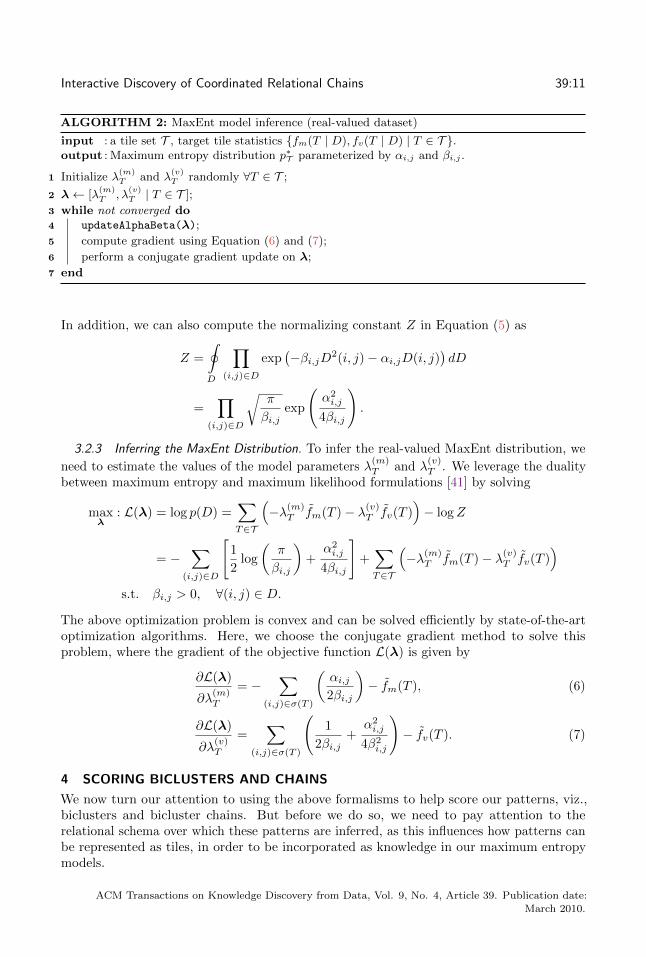
ALGORITHM 2: MaxEnt model inference (real-valued dataset)

input : a tile set T , target tile statistics {fm(T | D), fv(T | D) | T ∈ T }.output : Maximum entropy distribution p∗T parameterized by αi,j and βi,j .

1 Initialize λ(m)T and λ

(v)T randomly ∀T ∈ T ;

2 λ← [λ(m)T , λ

(v)T | T ∈ T ];

3 while not converged do4 updateAlphaBeta(λ);

5 compute gradient using Equation (6) and (7);

6 perform a conjugate gradient update on λ;

7 end

In addition, we can also compute the normalizing constant Z in Equation (5) as

Z =

∮D

∏(i,j)∈D

exp(−βi,jD2(i, j)− αi,jD(i, j)

)dD

=∏

(i,j)∈D

√π

βi,jexp

(α2i,j

4βi,j

).

3.2.3 Inferring the MaxEnt Distribution. To infer the real-valued MaxEnt distribution, we

need to estimate the values of the model parameters λ(m)T and λ

(v)T . We leverage the duality

between maximum entropy and maximum likelihood formulations [41] by solving

maxλ

: L(λ) = log p(D) =∑T∈T

(−λ(m)

T fm(T )− λ(v)T fv(T ))− logZ

= −∑

(i,j)∈D

[1

2log

(π

βi,j

)+

α2i,j

4βi,j

]+∑T∈T

(−λ(m)

T fm(T )− λ(v)T fv(T ))

s.t. βi,j > 0, ∀(i, j) ∈ D.

The above optimization problem is convex and can be solved efficiently by state-of-the-artoptimization algorithms. Here, we choose the conjugate gradient method to solve thisproblem, where the gradient of the objective function L(λ) is given by

∂L(λ)

∂λ(m)T

= −∑

(i,j)∈σ(T )

(αi,j2βi,j

)− fm(T ), (6)

∂L(λ)

∂λ(v)T

=∑

(i,j)∈σ(T )

(1

2βi,j+

α2i,j

4β2i,j

)− fv(T ). (7)

4 SCORING BICLUSTERS AND CHAINS

We now turn our attention to using the above formalisms to help score our patterns, viz.,biclusters and bicluster chains. But before we do so, we need to pay attention to therelational schema over which these patterns are inferred, as this influences how patterns canbe represented as tiles, in order to be incorporated as knowledge in our maximum entropymodels.


March 2010.

39:12 H. Wu et al.

4.1 Entity-Entity Relation Extraction

In this section, we describe the approach to construct a multi-relational schema S(U ,R)from a transaction data matrix D. Recall that whenever an element D(r, ei) has a non-zerovalue (e.g. 1 in the binary case or a fraction in the range of [0, 1] in the real-valued case), thisdenotes that entity ei appears in row r of D. As an example, when considering text data,an entity would correspond to a word or concept, and a row to a document in which thisword occurs. (Thus, note that when considering text data we currently model occurrencesof entities at the granularity of documents. Admittedly, this is a coarse modeling in contrastto modeling occurrences at the level of sentences, but it suffices for our purposes.)

To extract entity-entity relations from transaction data matrix D, we utilize the entityco-occurrence information. To be more specific, each binary relation in R stores the entityco-occurrences in data matrix D between two entity domains, e.g. for each R = R(Ui, Uj) inR, (e, f) ∈ R for e ∈ Ui, f ∈ Uj , and e and f appear at least once together in a row in D.

4.2 Background Model Definition

Next, to discover non-trivial and interesting patterns, we need to incorporate some basicinformation about the multi-relational schema S(U ,R) into the model. For such basicbackground knowledge over D we use the column marginals and the row marginals for eachentity domain. To this end, following Wu et al. [61] we construct a tile set Tcol consisting ofa tile per column, a tile set Trow consisting of a tile per row per entity domain, and a tileset Tdom consisting of a tile per entity domain but spanning all rows. Formally, we have

Tcol = {(UD, e) | e ∈ U,U ∈ U},Trow = {(r, U) | r ∈ UD, U ∈ U}, and

Tdom = {(UD, U) | U ∈ U}.

Here, UD represents the domain of all the documents in the dataset (e.g. the set of all rowsin the data matrix D). We refer to the combination of these three tile sets as the backgroundtile set Tback = Trow ∪Tcol ∪Tdom . Given the background tiles Tback , the background MaxEntmodel pback can be inferred using iterative scaling (see Sect. 3.1.3) and the conjugate gradientmethod (see Sect. 3.2.3) for binary and real-valued cases, respectively.

4.3 Quality Scores

To assess the quality of a given bicluster B with regard to our background knowledge, weneed to first convert it into tiles such that we can infer the corresponding MaxEnt model.Below we specify how we do this conversion for biclusters from entity-entity relations. For agiven bicluster B = (Ei, Ej), we construct a tile set TB consisting of |Ei| |Ej | tiles as

TB = {(rows(X;D), X) | X = {ei, ej} with (ei, ej) ∈ B} , (8)

where rows(X;D) is the set of rows that contain X in D, e.g. the corresponding entries forX in the matrix D that have non-zero values.

To evaluate the quality of a bicluster chain C, for each bicluster B ∈ C, we construct theset of tiles TB as illustrated by Equation (8), and the tile set that corresponds to a biclusterchain C is then TC =

⋃B∈C TB .

Next, we describe the metrics that measure how much information a bicluster B (or thecorresponding tile set TB) gives with regard to the background model pback . Motivated


March 2010.


by De Bie [9], the global score is defined as

sglobal(B) = KL(pB ||pback ) , (9)

where pB represents the MaxEnt distribution inferred over the background tile set Tback andthe tile set TB for the bicluster B.

For both of binary and real-valued MaxEnt model, the MaxEnt distribution p(D) can befactorized as

p(D) =∏

(i,j)∈D

p(D(i, j)) .

Thus, this global score can be written as

sglobal(B) =

∮D

pB(D) logpB(D)

pback (D)dD

=

∮D

∏(i,j)∈D

pB(D(i, j))∑

(i,j)∈D

logpB(D(i, j))

pback (D(i, j))dD

=∑

(i,j)∈D

∫ +∞

−∞pB(Di,j) log

pB(D(i, j))

pback (D(i, j))dD(i, j)

=∑

(i,j)∈D

KL(pB(D(i, j))||pback (D(i, j))) . (10)

For the binary MaxEnt model, D(i, j) follows the Bernoulli distribution

D(i, j) ∼ Bernoulli(q), where q =exp

(∑T∈T (i,j) λT

)exp

(∑T∈T (i,j) λT

)+ 1

,

and the global score for binary MaxEnt model would be

sglobal(B) =∑

(i,j)∈D

(qB log

qBqback

+ (1− qB) log1− qB

1− qback

).

For the real-valued MaxEnt model, D(i, j) follows the Gaussian distribution

D(i, j) ∼ N(− αi,j

2βi,j,

1

2βi,j

).

Given any two normal distribution PN1= N (µ1, σ

21) and PN2

= N (µ2, σ22), we can verify

that the KL-divergence between these two normal distribution is

KL(PN1||PN2

) = logσ2σ1

+σ21 + (µ1 − µ2)

2

2σ22

− 1

2. (11)

Combining Equation (10) and (11), the global score for the real-valued maximum entropymodel is

sglobal =∑

(i,j)∈D

1

2log

β(B)i,j

β(back)i,j

+β(back)i,j

2β(B)i,j

+ β(back)i,j

(α(back)i,j

2β(back)i,j

−α(B)i,j

2β(B)i,j

)2

− 1

2

. (12)

However, using the global score defined above requires us to re-infer the MaxEnt modelfor every candidate bicluster that needs to be evaluated, which could be computationallyexpensive and thus not applicable to our interactive mining sitting. Moreover, sglobal


March 2010.

39:14 H. Wu et al.

Fig. 3. Visual representations of a bicluster that includes three entities in D1 and three entities in D2.(A) displays all individual relationships between the two sets of entities from the two domains, D1 andD2. (B) Realtionships are aggregated as an edge bundle that represents a bicluster.

evaluates a candidate globally, whereas typically most information is local : at most a fewentries in the maximum entropy distribution will be affected by adding B into the model.Making use of this observation and considering the ease of computation, to reduce thecomputational cost of candidate bicluster evaluation, we define the score slocal(B) thatmeasures the local surprisingness of a tile set as

slocal(B) = −∑T∈TB

∑(i,j)∈σ(T )

log pback (D(i, j)) , (13)

which is an approximation of the local negative log-likelihood of the bicluster B. For bothbinary and real-valued MaxEnt model, pback (D(i, j)) indicates the probability (or probabilitydensity) evaluated at the value D(i, j) under the current background MaxEnt model. Noticethat although the global and local scores are described using the notation of biclustershere, they can also be directly adopted to assess the quality of bicluster chains becausefundamentally these scores are defined around the concept of tiles and bicluster chains (andcan thus be trivially converted to a set of tiles as described at the beginning of this section).

5 MERCER

MERCER is a visual analytics system, supported by the maximum entropy model above, tosupport interactive exploration of coordinated relationships using biclusters. Coordinatedrelationships are groups of relations, connecting sets of entities from different domains(e.g., people, location, organization, etc.), which potentially indicate coalitions betweenthese entities. MERCER extends a recently proposed bicluster visualization, BiSet [51], byincorporating MaxEnt models to support user exploration of entity coalitions for sensemakingpurposes. In this section, we first briefly introduce BiSet, followed by the enhancements thatMERCER provides.

5.1 BiSet Technique Overview

The key idea is that BiSet visualizes the mined biclusters in context as edge bundles betweensets of related entities. BiSet uses lists as the basic layout to present entities and biclusters.Figure 3 shows an example of a visualized bicluster in BiSet. In Figure 3, (A) shows allindividual edges between related entities and (B) presents the same bicluster as an edgebundle. BiSet enables both ways to show the coalition of entities with two modes: linkmode and bicluster mode. Link mode displays the individual connections among entitiesin a dataset, while bicluster mode offers a more clear representation to show identifiedbiclusters in the dataset. Based on these visual representations, BiSet can visually show


March 2010.


Fig. 4. An example of four bicluster-chains (b1 - b4, b2 - b4, b2 - b5 and b3 - b5). These chainsconsist of entities from three domains, D1, D2 and D3. b1 and b4 are connected through e1. b2 andb4 share e1 and e2. b2 and b5 are linked by e3. b3 and b5 are connected by e3 and e5.

bicluster-chains as connected edge bundles through their shared entities. Figure 4 shows fourbicluster-chains (b1 - b4, b2 - b4, b2 - b5 and b3 - b5) visualized using BiSet. Each of themconsists of two different biclusters including entities from three domains. The two biclustersin each chain are visually connected through one or two shared entities. For example,bicluster b2 and b4 are connected by entity e1 and e2. With edges, BiSet enables users tosee members of bicluster-chains and how these biclusters are connected. This potentiallyguides users to interpret the coalition among sets of entities from multiple domains in anorganized manner (e.g., checking connected biclusters from left to right).

To support exploratory analysis, BiSet treats edge bundles as first class objects, so userscan directly manipulate them (e.g., drag and move) to spatially organize them in meaningfulways. BiSet also offers automatic ordering for entities and biclusters to help users organizethem. For example, entities can be ordered based on their frequency in a dataset andbiclusters can be ordered by size (i.e., the number of entities participating in a bicluster).Moreover, BiSet can highlight bicluster-chains as users select their members (e.g., entitiesand biclusters). This provides visual clues for users to follow in conducting their analysis.

5.2 Adaptions from BiSet to MERCER

Key adaptions, from BiSet to MERCER, lie in two levels: representation-level (specificallyvisual encoding), and interaction-level, (human-model interaction, in particular). MERCERshares the basic visual encodings in shape and size (to represent entities, biclusters and edges)with BiSet, but it introduces surprisingness oriented highlighting, which is not included inBiSet. Detailed visual encodings in MERCER is discussed in Section 5.3. This surprisingnessoriented highlighting aims at supporting human-model interactions in MERCER. Thecapability of enabling human-model interactions is the essential difference between BiSet andMERCER. This capability helps to address recently identified usability challenges of usingbiclusters for sensemaking (e.g., bicluster evaluation and prioritization) [49, 52]. Withouthuman-model interactions, in BiSet, users have to check biclusters or bicluster-chains (basedon connection oriented highlighting) and manually figure out potentially useful ones. Thismay take much cognitive effort, especially when data is large. However, in MERCER, users


March 2010.

39:16 H. Wu et al.

Fig. 5. Detailed visual encodings in MERCER. 1a, 2a and 3a depict the normal state of an entity, abicluster and edges, respectively. 1b, 2b and 3b depict the connection-oriented highlighting state of anentity, a bicluster and edges, when users select bicluster 2c, hover over entity 1f and select entity 1c.1e, 2d and 3c illustrate the surprisingness-oriented highlighting state of an entity, a bicluster and edges.1d demonstrates larger fonts of entities as users hover the mouse pointer over their previously selectedentity 1c. Moreover, 2e represents a bicluster (in the normal state) with its edges chosen to be hiddenby users.

can explicitly request computation to help them find potentially useful biclusters or bicluster-chains, by directly interacting with a bicluster. Moreover, by revealing the surprisingnessoriented highlighting, MERCER helps to prioritize biclusters and bicluster-chains to supportuser explorations. The human-model interaction capability and evaluation strategies arediscussed in Section 5.4 and Section 5.5, respectively.

5.3 MERCER Visual Encoding

5.3.1 Shape and Size. In MERCER, entities and biclusters are represented as rectangles(e.g., 1a and 2a in Figure 5), and edges are visualized as Bezier curves. We use Bezier curvesbecause they can generate more smooth edges, compared with polylines [32]. Rectanglesindicating entities are equal in length, while those representing biclusters are not. MERCERapplies a linear mapping function to determine the length of a bundle based on the totalnumber of its related entities. In a bicluster rectangle, MERCER uses two colored regions(light green and light gray) to indicate the proportion between its related entities in listsof both sides (left and right). In an entity rectangle, a small rectangle is displayed on theleft to indicate its frequency in a dataset. The length of these rectangles is determinedby the frequency of the associated entities with a linear mapping function. These helpsusers to visually discriminate entities from biclusters. Moreover, when users hover overa selected entity or bicluster (e.g., entity 1c and bicluster 2c in Figure 5), the font of itsrelated entities is enlarged (e.g., comparing 1d with 1b in Figure 5). This helps users reviewrelevant information of their previous selections.

5.3.2 Color Coding. MERCER applies color coding to entities, biclusters and edges toindicate their states and allows users to hide edges of biclusters to reduce visual clutter (see2e in Figure 5). In MERCER, entities, biclusters and edges have two basic states: normal


March 2010.


Fig. 6. The human-model interaction flow in MERCER. Visual representations in MERCER enable theinteraction between users and the proposed maximum entropy models.

and highlighted. The normal state is the default state for entities, biclusters and edges.Examples of the normal state for them are shown as 1a, 2a and 3a, respectively, in Figure 5.To encode surprisingness, MERCER supports two types of highlighting states: connectionoriented highlighting (colored as orange in Figure 5) and surprisingness oriented highlighting(color as red in Figure 5), which encode two levels of information: the coalition of entities andthe surprisingness of the coalition. The former indicates the linkage of entities, emphasizingthe connections between entities. The latter reveals the model-evaluated surprisingness ofdifferent sets of entity coalitions. In Figure 5, examples of connection-oriented highlightingfor entities, biclusters and edges are shown as 1b, 2b and 3b, respectively; while examples ofsurprisingness-oriented highlighting are presented as 1e, 2d and 3c.

The connection oriented highlighting state is triggered as users hover or select an entity ora bicluster. For example, when users hover the mouse pointer over the entity 1f, its directlyconnected bicluster 2b is highlighted and other entities that belong to this bicluster arealso highlighted. The surprisingness oriented highlighting state is triggered by explicit userrequest of model evaluation. For instance, in Figure 5, as users request to find the mostsurprising chains with bicluster 2c as the starting point, MERCER highlights entities andbiclusters in a chain that has the highest score given by the proposed maximum entropymodel (the approach to discover such a chain will be described in Section 5.5 below). Withour color codings, MERCER empowers users to explore entity coalitions by directing themto computationally identified surprising chains.

5.4 Human-model Interaction

MERCER allows human-model interaction with visualizations to support visual analytics ofentity coalitions. To enable this capability, we incorporate the proposed maximum entropymodels into MERCER. Figure 6 illustrates the human-model interaction flow in MERCER.Visual representations in MERCER work as the bridge to enable the interaction betweenusers and the proposed models. After inspecting the visualized biclusters and bicluster-chains,users can explicitly request model evaluations using right click menus on a bicluster. Thisfurther triggers the maximum entropy model to evaluate either all paths passing throughthe requested bicluster or its neighboring biclusters. Then, based on results of the modelevaluation, MERCER highlights the most surprising bicluster-chain including the userrequested bicluster or neighboring biclusters. We address this with a detailed discussion inSection 5.5. Moreover, users can mark highlighted bicluster(s), based on model evaluation,as useful one(s) by using a right click menu on the bicluster(s). This implicitly evokes amodel update function, which informs the model that the information in a marked biclusterhas been known by users. Then the model updates its background information to take the


March 2010.

39:18 H. Wu et al.

marked bicluster(s) into account and prepare for further user requested evaluations. Thishuman-model interaction flow in MERCER enables the combination the human cognitionwith computations for the exploration of entity coalitions.

5.5 Model Evaluation Strategies

MERCER offers two strategies to evaluate bicluster-chains, using the proposed maximumentropy models, based on explicit user requests: full path evaluation and stepwise evaluation.Both ways require users to explicitly specify a bicluster based on its visual information, e.g.size of a bicluster, frequency of corresponding entities, etc., to initiate the chain. The formerevaluates all bicluster-chains passing through the bicluster that users request for evaluation,while the latter evaluates neighboring biclusters that satisfy a certain degree of overlap withthe user-specified one. MERCER enables users to explicitly issue an evaluation request froma bicluster with a right click menu. From the menu, users can choose the desired way ofevaluation.

5.5.1 Full Path Evaluation. The full path evaluation in MERCER includes three key steps:1) path search, 2) path evaluation, and 3) path rank. In MERCER, a path, passing througha bicluster, refers to a set of biclusters (e.g., {b2, b4} in Figure 4), which can be connectedthrough certain entities to form a bicluster-chain. In the path search step, MERCER findsall possible paths passing through the bicluster that users request for evaluation. Similarto tree search, MERCER treats the user requested bicluster as a root node and appliesdepth-first search to find all paths starting from this bicluster. If the user requested biclusteris not from the left or right most relation in the user specified multi-relational schema,MERCER performs bidirectional search and then combines identified paths in the left andthose in the right together to obtain all paths going through this bicluster. Then in the pathevaluation step, MERCER converts each bicluster-chain, found in the previous step, intoa unique set of tiles following the Equation (8) in Section 4.3, and applies the maximumentropy models to score them. Finally, based on the score from the model, in the path rankstep, MERCER ranks these bicluster-chains and visually highlights the one that has thehighest score (e.g., {2c, 2d} in Figure 5). Thus, with the full path evaluation in MERCER,users can get the most surprising bicluster-chain for the bicluster requested for evaluation.

5.5.2 Stepwise Evaluation. The stepwise evaluation in MERCER examines neighboringbiclusters for the one that users request for evaluation. Neighboring biclusters for a specificbicluster refers to those that can meet certain degree of overlaps, with respect to participatedentities, with a user requested bicluster. MERCER uses the Jaccard coefficient to measurethe degree of overlaps between two biclusters with a default threshold set as 0.1. Thus, for aspecific bicluster, its potential neighboring biclusters are those sharing at least one domain(e.g., people, location, date, etc.) with this one.

Similar to the full path evaluation, the stepwise evaluation also has three key steps,including: 1) neighboring bicluster search, 2) neighboring bicluster evaluation, and 3)neighboring bicluster coloring. Based on a user specified bicluster for evaluation, MERCERfirst identifies its neighboring biclusters using the Jaccard coefficient. Then, MERCERconverts the identified neighboring biclusters into different sets of tiles following Equation (8)and employs the maximum entropy models to score them. Based on the model evaluationscore, BiSet applies a linear mapping function to assign the opacity value of surprisingnessoriented highlighting color to these biclusters. The more red a color is, and the higherscore this neighboring bicluster gets, which indicates more surprising information. Figure 7


March 2010.


Fig. 7. Exampled results from the stepwise evaluation in MERCER. (a) shows the bicluster selected by auser to initiate the maximum entropy model evaluation. (b) represents the most surprising bicluster inthe same bicluster list as the one requested for evaluation. (c) illustrates the most surprising bicluster inanother bicluster list.

Fig. 8. Document view mode in MERCER. (A) depicts the bicluster ID, relevant document ID(s) andassociated entities. (B) shows the content of a document. (C) lists all document IDs in a dataset with asearch function.

gives an example of the stepwise evaluation in MERCER. In this example, users request toevaluate a bicluster (see a), MERCER highlights neighboring biclusters based on their modelevaluation scores. Of these highlighted biclusters, bicluster b shows the most surprisingone in the same bicluster list as that requested for evaluation, and bicluster c is the mostsurprising bicluster in the adjacent bicluster list. Although bicluster b here could not beused to extend the users selected bicluster a, it has the potential to reveal entities related tothe bicluster a and the plots. Thus, we also take the most surprising bicluster from the samerelation of the users selected bicluster into account. Such stepwise evaluation potentiallyenables to involve users in the process of building a meaningful bicluster-chain. Each timeafter a stepwise evaluation, users can investigate highlighted neighboring biclusters, identifyand then select useful one(s) for further exploration. Users can iterate this process and builda bicluster-chain that is meaningful for them.


March 2010.

39:20 H. Wu et al.

5.6 Bicluster based Evidence Retrieval

In MERCER, users can directly retrieve related documents from biclusters by using a rightclick menu. Users can use a right click menu to open a popup view, where relevant documentsare listed, as is shown in Figure 8. This helps users review information relevant to thisbicluster and verify computationally identified coalitions of entities. This document view ison top of the relationship exploration view with transparency, so users can simultaneouslysee both the visualized relationships and corresponding documents. Moreover, after readingdocuments, users can quickly return to the relationship exploration view by closing it.

6 EXPERIMENTS

We describe the experimental results over both synthetic and real datasets. For real datasets,we focus primarily on datasets from the domain of intelligence analysis. Through a casestudy, we demonstrate how the proposed maximum entropy models embedded in our visualanalytics approach helps analysts to explore text datasets, such as used in intelligenceanalysis. All experiments described in this section were conducted on a Xeon 2.4GHzmachine with 1TB memory. Performance results (for synthetic data) were obtained byaveraging over 10 independent runs.

6.1 Results on Synthetic Data

To evaluate the runtime performance of the proposed maximum entropy models with respectto the data characteristics, we generate synthetic datasets. Since we focused on the runtimeperformance of the proposed models here, and the multi-relational schema of the dataset willnot affect how the proposed models are inferred over the data matrix D, we will temporarilyignore the multi-relational schema of the dataset in the synthetic data for now. The syntheticdatasets are parameterized as follows. The data matrix D consists of N rows and M columns,or entities, and β denotes the density of the data matrix D. For each entry in the datamatrix D, we set its value to be non-zero with probability β. For the binary case, thenon-zero values would naturally be one, and for the real-valued case, the non-zero valuesare generated from a standard uniform distribution. In order to avoid the scenario that toomany rows or columns in D contains only zeros, a non-zero value is placed randomly in arow or column if it only contains zeros.

In our experiments, we explore data matrix D sizes of (N = 1000,M = 1000), (N =2000,M = 2000), and (N = 3000,M = 3000), and varied the density β of the data matrixD from 0.01 to 0.05 in steps of 0.01. To infer the maximum entropy models, we use columnmargin and row margin tiles as the set of constraint tiles for the proposed model (see Sect. 3).We first investigate the time needed to infer the maximum entropy models. Figure 9 showsthe model inference time for the binary and real-valued maximum entropy formulations.As expected, model inference increases with dataset size and requires more time for thereal-valued model. Since the real-valued maximum entropy model adopts the conjugategradient method, model inference time heavily depends upon the structure of the givendataset, the number of constraint tiles, and how fast the model converges to the optimalsolution along the gradient direction. For example, in our experiments we used the rowand column margin tiles as the constraints for the real-valued maximum entropy model,the dimension of the gradient could be 2(M + N) (that would be 4,000 dimension whenN = 1000,M = 1000 for our synthetic datasets).

Another interesting phenomenon we observed here is that as the density β of the datamatrix D increases, the inference time required by the real-valued maximum entropy model


March 2010.


Fig. 9. Time to infer the binary (left) and real-valued (right, Y-axis is in log scale) maximum entropymodel on synthetic datasets. The error bars represent the standard deviation

Fig. 10. Time to evaluate a set of tiles with the binary (left) and real-valued (right) maximum entropymodel on synthetic datasets. The set of solid lines on the top represents the results of global score, andthe set of dash lines at the bottom represents the results of local score. The error bars represent thestandard deviation, and the Y-axis is in log scale.

decreases. One explanation for this phenomenon is that denser data matrices providemore information to the maximum entropy model about the underlying data generationdistribution through the constraint tiles. This aids the model in rapidly learning the structureof the data space and search for the optimal solution with fewer iterations of the conjugategradient algorithm.


March 2010.

39:22 H. Wu et al.

We also measured the runtime performance of evaluating tile sets with the proposedbinary and real-valued maximum entropy models since the patterns (biclusters or biclusterchains) whose qualities we would like to assess will eventually be converted into a set oftiles in our framework. To be more specific, we randomly generated a set of tiles over thesynthetic data matrix, and compared the time required to evaluate this tile set with bothglobal score and local score using converged binary and real-valued models, and Figure 10illustrates the results. As we can see from this figure, in both binary and real-valuedmaximum entropy model, evaluating tile sets using the global score requires more time thanthe local score, which is expected since the global score requires a complete re-inferenceof the model. The difference of runtime performance between global and local scores issignificant in the real-valued model due to this model inference step. When applying the real-valued maximum entropy model in practical applications, such as the one here necessitatingreal-time interaction, we can employ an asynchronized model inference scheme, e.g. creatinga daemon process to infer the model when the system is idle, and adopt the local score toevaluate tile sets.

6.2 Evaluation on Real Dataset: A Usage Scenario

In this section, we walk through an intelligence analysis scenario to demonstrate howMERCER, particularly incorporating the proposed maximum entropy models for identifyingsurprising entity coalitions, can support an analyst to discover a coordinated activity viavisual analysis of entity coalitions. For ease of description, we use a small dataset, viz.The Sign of the Crescent [22], which includes 41 fictional intelligence reports about threecoordinated terrorist plots in three cities. Each plot involves at least four suspicious people.24 of these reports are relevant to the plots. We use LCM [58] to identify closed biclustersfrom this dataset with the minimum support parameter set to 3. This assures that eachbicluster has at least three entities from one domain. This generates 337 biclusters from284 unique entities and 495 individual relationships (based on entity co-occurrence in thereports).

In order to try to discover all the possible plots hidden in the Crescent dataset, inMERCER, we set the threshold for the Jaccard coefficient as 0.05, which is a loose constraint.This enables the model to evaluate those neighboring biclusters that has a few entity overlapswith user specified biclusters for assessment. Although MERCER fully supports patternevaluations with the real-valued maximum entropy model, we observed that the modelevaluation results of a given bicluster were similar when using the binary and the real-valuedmaximum entropy models in our experiments over the Crescent dataset. Thus, we onlypresent the use case study using the binary maximum entropy model here to demonstratethe effectiveness of the proposed MERCER technique when assisting analysts in conductingintelligence analysis tasks.

To illustrate the benefits of integrating the maximum entropy models into visual analytictools, in this intelligence analysis scenario, we use BiSet [51] as the baseline approach forcomparison purposes. Notice that BiSet does not has the capability of model evaluations,and thus it just provides the connection oriented highlighting function for users to manuallyexplore entity coalitions. We begin our discussions with the use case of BiSet, and thendiscuss the use case of MERCER.

In our scenario, suppose that Linda is an intelligence analyst. She has a task to readintelligence reports and identify potential terrorist threats and key persons from the Crescentdataset. She opens BiSet, picks four identified domains (people, location, phone number and


March 2010.


date), and starts her analysis. Figure 11 to Figure 16 demonstrate Linda’s key analyticalsteps using BiSet. Figure 17 and Figure 18 show the key steps of Linda’s analytical processusing MERCER. The BiSet use case and Figure 17 are informed by the previous publicationof the BiSet technique [51].

6.2.1 BiSet Use Case. Linda starts analysis by checking people’s names. When she hoversthe mouse over an entity, BiSet highlights its related bundles and entities. Immediately shenotices that A. Ramazi is active in three bundles. This indicates that he may be involvedin three coordinated activities. Linda selects it (Figure 11) to focus on the highlightedentities of these bundles. She finds that A. Ramazi is involved in two cells with five people(S. Khallad, T. al Adel, B. Dhaliwal, C. Webster and F. Goba). One cell is in Germanyand the other cell is more broadly located in four countries. A. Ramazi is the only personconnecting the two cells. Moreover, two overlapped groups of people (sharing A. Ramaziand C. Webster) are involved in the broader cell, and each group has its unique person, B.Dhaliwal and F. Goba, respectively.

Fig. 11. Selecting A. Ramazi and finding that there are two similar bundles and two cells.

Then Linda decides to investigate the two overlapped groups, since she aims to knowwhat brings the unique people to them. She checks B. Dhaliwal first. After hovering themouse over it, two bundles are highlighted. Following their edges, Linda finds that twopeople’s names (B. Dhaliwal and C. Webster) and four locations (Charlottesville, Virginia,Afghanistan and Richmond) are shared by them, and the bigger one is connected with anew name, H. Pakes (see Figure 12). Then she checks F. Goba in the same way. This timethree names (M. Galab, Y. Mosed and Z. al Shibh) and three bundles are highlighted, andone name, M. Galab, has a high frequency (see Figure 13).

Linda quickly notices this, so she decides to temporarily pause her analysis of B. Dhaliwal,and moves on with F. Goba. Linda hovers the mouse over M. Galab to check what additionalinformation it can lead to. However, no additional bundles or names are highlighted. Lindarealizes that people potentially connected with M. Galab have already been highlighted inthe current view. The bundle (shown in Figure 13 as the black box in the middle) revealstwo people (F. Goba and Y. Mosed) related with M. Galab, and all their activities are inthe US, including Charlottesville, Virginia, Atlanta, Los Angeles, New Orleans and Georgia.Linda get this key insight based on the group of locations in this bundle. The relationsfrom this bundle are important, and Linda hypothesizes that the three people (M. Galab, Y.


March 2010.

39:24 H. Wu et al.

Fig. 12. When hovering the mouse over B. Dhaliwal, one name and two bundles are highlighted.

Fig. 13. When exploring F. Goba, three names and three bundles are highlighted.

Mosed and Z. al Shibh) may work on something together in the US. Thus, by following thistail [25], she wants to find more related information.

After Linda selects this useful bundle, BiSet highlights its related bundles that can formbicluster chains. Five bundles, between the location list and the phone number list, arehighlighted (Figure 14), and two bundles, between the phone number list and the datelist, are highlighted (Figure 15). Relevant entities in these lists are also highlighted. Forthese newly highlighted bundles, Linda finds that there are two big ones (relatively longershown in Figure 14 and Figure 15). These two bundles seem useful since they have morerelations. Linda decides to check them and find how bundles from different relationship lists


March 2010.


Fig. 14. After selecting a useful bundle, five bundles (in-between the list of location and phone number)are highlighted. Checking connected entities of the first and the third bundles.

Fig. 15. After selecting a useful bundle, two bundles (in-between the list of phone number and date)are highlighted.

are connected. For bundles between the location list and the phone number list (from topto bottom in Figure 14), Linda finds that the first and the third bundle share two locations(Charlottesville and Virginia) with the selected bundle, and other highlighted bundles justshare one location with the selected one. Compared with the first bundle, the third oneis related with less locations that are not associated the selected bundle. Linda choosesto focus on information highly connected with the selected bundle, instead of additionalinformation, so she considers the third bundle a useful one. Using a similar strategy inanother bicluster list (between the phone number list and the date list), she finds that thebigger bundle (the top listed one in Figure 15) is more useful.

After this, Linda uses the right click menu to hide edges of other bundles for creating aclear view (see Figure 16). Then, in her workspace, there are three bundles connecting witheach other through two shared locations (Charlottesville and Virginia) and three sharedphone numbers (703-659-2317 and 804-759-6302 and 1070173). Linda feels that she hasfound a good number of relations, connecting four groups of entities, which may reveal asuspicious activity. Therefore, she decides to read relevant documents to collect detailsabout these connections and make her hypothesis.

These three connected bundles direct Linda to eight reports, and all of them are relevantto the plot. By referring to the entities with bright shading in the four connected groups(shown in Figure 16), Linda reads these reports. The darker shading indicates that an entityis shared more times. This information helps to direct her attention to more important


March 2010.

39:26 H. Wu et al.

entities in the reports. After reading these reports, she identifies four key persons involvedin a potential threat as follows:

F. Goba, M. Galab and Y. Mosed, following the commands from A. Ramazi,plan to attack AMTRAK Train 19 at 9:00 am on April 30.

In this use case, Linda has to manually check details about shared entities to determinewhich biclusters are meaningful and useful, because BiSet does not provide the functionof model based bicluster or chain evaluation. With just connection oriented highlighting,Linda has to verify many connected biclusters to find potentially useful ones. This limits heranalysis strategy as stepwise search, and such search focuses on checking the shared entitiesof investigated biclusters. Thus, it takes Linda significant effort to work at the entity-levelinformation to identify a meaningful bicluster chain.

6.2.2 MERCER Use Case. Similar to the previous case, Linda begins analysis by hoveringindividual entities in the list of people. MERCER highlights related bundles and entities asshe hovers the mouse over an entity. Immediately she finds that A. Ramazi is active in threebundles (Figure 17 (1)), which indicates that this person is involved in three coordinatedactivities. Based on edges, Linda finds that two bundles are similar (see the black dottedbox in Figure 17 (1)) due to the number of their shared entities. Thus, she decides to furtherinvestigate them.

With the right click menu on the two bundles, Linda uses the stepwise evaluation function,provided by MERCER, to find their neighboring bundles that contain the most surprisinginformation (Figure 17 (2) and (3)). Based on evaluated scores from the maximum entropymodel, MERCER highlights their most surprising neighboring bundles. She finds that themost surprising bundles connected with the two investigated bundles are the same. Thisindicates that the model-suggested most surprising bundle may be important and worthy offurther inspection, and so Linda decides to find more relevant information from it.

Linda chooses the full path evaluation function on this model-suggested bundle to findthe most surprising bicluster-chain. MERCER highlights the path (Figure 17 (4)) passingthrough this bundle having the highest evaluation score from the maximum entropy model.This provides four connected sets of entities from all the selected domains (people, location,phone and date). Linda feels that she has discovered enough information for a story, so shechecks entities involved in this chain and reads documents from the three connected bundles.The three bundles directs Linda to nine reports in total, and eight of them are relevant toeach other. After reading these relevant reports, she identifies a potential threat with fourkey persons as follows:

F. Goba, M. Galab and Y. Mosed, following the commands from A. Ramazi,plan to attack AMTRAK Train 19 at 9:00 am on April 30.

Linda is satisfied with this finding and marks the bundles in this model suggested chainas useful, using the right click menu. This informs the integrated maximum entropy modelin MERCER that the information in these bundles has been known to the analyst, and sothe model updates its background information for further evaluations.

The content of one report, from the bundle in the middle of the surprising chain (ain Figure 17 (4)), is irrelevant to that of the other eight, but the entities extracted fromthis report are connected with those in the identified threat. Thus, Linda considers theinformation in this report as potentially useful clues, which may lead to some other threatplot(s). In order to check what new information it can bring in, she uses the full pathevaluation function on the bundle in the middle of the surprising chain (a in Figure 17


March 2010.


Fig

.16

.U

sin

ga

righ

t-cl

ick

men

ufr

omed

geb

un

dle

sto

hid

eed

ges.

Ref

erri

ng

toth

efo

ur

con

nec

ted

grou

ps

ofu

sefu

len

titi

es,

thro

ugh

thre

eb

un

dle

s(a

,b

andc

),fo

rh

ypo

thes

isg

ener

atio

n.

Th

ese

enti

ties

are

tho

sein

sid

eth

eb

oxes

wit

hd

ott

edb

ord

ers.


March 2010.

39:28 H. Wu et al.

Fig

.1

7.

Apro

cesso

ffi

nd

ing

on

em

ajorth

reatp

lot

with

keystep

s.(1

):B

asedo

nA.Ram

azi,fi

nd

ing

that

there

aretw

osim

ilarb

un

dles.

(2):

Fin

din

gth

em

ost

surp

rising

bu

nd

leevalu

atedb

yth

emaxim

um

entro

pymodel

foro

ne

of

the

two

similar

bu

nd

les.(3

):F

ind

ing

the

mo

stsu

rprisin

gb

un

dle

evaluated

by

themaxim

um

entro

pymodel

forth

eo

ther

on

eo

fth

etw

osim

ilarb

un

dles.

(4).

Th

em

ost

surp

rising

biclu

ster-chain

sug

gested

by

the

maxim

um

entro

pymodel

forth

em

ost

surprisin

gb

un

dle

iden

tified

inprevio

us

steps.


March 2010.


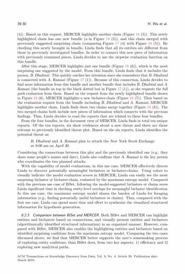
Fig

.1

8.

Ap

roce

sso

ffi

nd

ing

ano

ther

key

thre

atp

lot.

(5):

Fin

din

gth

em

ost

surp

risi

ng

bic

lust

er-c

hai

nb

yth

emaxim

um

entropymodel

fro

mth

eb

un

dle

mar

ked

inth

eb

lack

do

tted

box

.(6

):R

equ

esti

ng

thestepwise

eval

uat

ion

on

the

bu

nd

lea

in(5

).(7

):B

ased

on

the

mo

stsu

rpri

sin

gb

un

dle

show

nin

(6),

req

ues

tin

gto

fin

dit

sm

ost

surp

risi

ng

bic

lust

er-c

hai

n.

(8):

Bas

edon

the

shar

eden

tity

,B.Dhaliwal

,re

qu

esti

ng

tofi

nd

the

mos

tsu

rpri

sin

gb

iclu

ster

-ch

ain

fro

mth

eb

un

dle

that

incl

ud

esB.Dhaliwal

andA.Ram

azi.

Th

ech

ain

fro

mth

isst

epan

dth

atfr

om

the

prev

iou

sst

epm

erg

eto

get

her

.


March 2010.

39:30 H. Wu et al.

(4)). Based on this request, MERCER highlights another chain (Figure 18 (5)). This newlyhighlighted chain has one new bundle (a in Figure 18 (5)), and this chain merged withpreviously suggested surprising chain (comparing Figure 17 (4) with Figure 18 (5)). Bychecking this newly brought in bundle, Linda finds that all its entities are different fromthose in previously investigated bundles. In order to connect this new piece of informationwith previously examined pieces, Linda decides to use the stepwise evaluation function onthis bundle.

After this stage, MERCER highlights just one bundle (Figure 18 (6)), which is the mostsurprising one suggested by the model. From this bundle, Linda finds that it includes theperson, B. Dhaliwal. This quickly catches her attention since she remembers that B. Dhaliwalis connected with A. Ramazi (Figure 17 (1)). Because of this connection, Linda decides tofind more information from this bundle and another bundle that includes B. Dhaliwal and A.Ramazi (the bundle on top in the black dotted box in Figure 17 (1)), so she requests the fullpath evaluation from them. Based on the request from the newly highlighted bundle shownin Figure 18 (6), MERCER highlights a new bicluster-chain (Figure 18 (7)). Then based onthe evaluation request from the bundle including B. Dhaliwal and A. Ramazi, MERCERhighlights another chain. Linda finds these two chains merge together (Figure 18 (8)). Thetwo merged chains both include new pieces of information which connects with the previousfindings. Thus, Linda decides to read the reports that are related to these four bundles.

From the four bundles, in the document view of MERCER, Linda finds in total ten uniquereports. Of the ten reports, six show evidences about a new threat and three are thoserelevant to previously identified threat plot. Based on the six reports, Linda identifies thepotential threat as:

B. Dhaliwal and A. Ramazi plan to attack the New York Stock Exchangeat 9:00 am on April 30.

Considering the connections between this plot and the previously identified one (e.g., theyshare some people’s names and date), Linda also confirms that A. Ramazi is the key personwho coordinates the two planned attacks.

With the capability of model evaluations, in this use case, MERCER effectively directsLinda to discover potentially meaningful biclusters or bicluster-chains. Using colors tovisually indicate the model evaluation scores in MERCER, Linda can easily see the mostsurprising bicluster or bicluster-chain, evaluated by the maximum entropy model. Comparedwith the previous use case of BiSet, following the model-suggested biclusters or chains savesLinda significant time in checking entity-level overlaps for meaningful bicluster identification.In this use case, the maximum entropy model shares the burden of Linda for foraginginformation (e.g., finding potentially useful biclusters or chains). Thus, compared with thefirst use case, Linda can spend more time and effort to synthesize the visualized structuredinformation for hypothesis generation.

6.2.3 Comparison between BiSet and MERCER. Both BiSet and MERCER can highlightentities and biclusters based on connections, and visually present entities and biclusters(algorithmically identified structured information) in an organized manner. However, com-pared with BiSet, MERCER also enables the highlighting entities and biclusters based onidentified surprising coalitions from the maximum entropy model. Comparing the two casesdiscussed above, we find that MERCER better supports the user’s sensemaking processof exploring entity coalitions, than BiSet does, from two key aspects: 1) efficiency and 2)exploring new analytical paths.


March 2010.


Compared with BiSet, MERCER more effectively directs users’ attention to potentiallyuseful biclusters or bicluster-chains by visually prioritizing them with colors based on theirmaximum entropy model evaluation scores. The model evaluation function provided inMERCER eases the process for users to find useful biclusters, particularly compared withmanually entity overlap investigation. For example, in the first use case, a user has toexamine in total 9 biclusters (4 in the left most bicluster list, 5 in the middle bicluster listand 2 in the right most bicluster list as shown in Figure 16), before she finally identifies ameaningful bicluster-chain that covers the information of a potential threat. However, inthe second use case, MERCER directs the user to a bicluster-chain after she investigates 3biclusters (in the left most bicluster list shown in Figure 17). Although this chain is slightlydifferent from the manually identified one in the first use case, it covers the same amount ofinformation as the other one does. Thus, in the second use case, MERCER saves the userfrom checking highlighted biclusters in the other two lists, and effectively provides a usefulbicluster-chain for users to explore.

Based on the four user selected domains (visualized as a fixed schema), it is hard toidentify all three threat plots in the Crescent dataset because not all pre-identified biclusterscan be shown. However, from the two cases, we can find that MERCER can direct usersfrom one identified plot to a new plot via a surprising bicluster-chain. However, when usersmanually forage relevant information, it is not easy for them to make such transitions dueto cognitive tunneling [56]. In the first use case, the key bundle that can lead to a new plotis actually identified not as useful as the one shown as b in Figure 16. Thus, MERCERsignificantly aids in identifying coalitions of entities worthy of further exploration.

7 RELATED WORK

In this section we survey related work. In particular, we discuss work related with regard tomining surprising patterns, iterative data mining, mining multi-relational datasets, findingplots in data, and bicluster visualizations for data exploration.

7.1 Mining Biclusters

Mining biclusters is an extensively studied area of data mining, and many algorithms formining biclusters from varied data types have been proposed, e.g. [2, 5, 39, 42, 57, 59, 63].Bicluster mining, however, is not the primary aim in this paper; instead it is only a componentin our proposed framework. Moreover, the above mentioned studies do not assess whetherthe mined clusters are subjectively interesting. A comprehensive survey of biclusteringalgorithms was given by Madeira and Oliveira [34].

7.2 Mining Surprising Patterns

There is, however, significant literature on mining representative/succinct/surprising patterns[e.g., 27] as well as on explicit summarization [e.g., 8]. Wang and Parthasarathy [60]summarized a collection of frequent patterns by means of a row-based MaxEnt model,heuristically mining and adding the most significant itemsets in a level-wise fashion. Tatti[54] showed that querying such a model is PP-hard. Mampaey et al. [35] gave a convexheuristic, allowing more efficient search for the most informative set of patterns. De Bie[10] formalized how to model a binary matrix by MaxEnt using row and column marginsas background knowledge, which allows efficient calculation of probabilities per cell in thematrix. Kontonasios et al. [28] first proposed a real-valued MaxEnt model for assessingpatterns over real-valued rectangular databases. These papers all focus on mining surprising


March 2010.

39:32 H. Wu et al.

patterns from a single relation. They do not explore the multi-relational scenario, and canhence not find connections among surprising patterns from different relations—the problemwe focus on.

7.3 Iterative Data Mining

Iterative data mining as we study was first proposed by Hanhijarvi et al. [18]. The generalidea is to iteratively mine the result that is most significant given our accumulated knowledgeabout the data. To assess significance, they build upon the swap-randomization approach ofGionis et al. [15] and evaluate empirical p-values. With the help of real-valued MaxEnt model,Kontonasios et al. [30] proposed a subjective interestingness measure called Information Ratioto iteratively identify and rank the interesting structures in real-valued data. Mampaeyet al. [35] and Kontonasios et al. [30] show that ranking results using a static MaxEntmodel leads to redundancy in the top-ranked results, and that iterative updating provides aprincipled approach for avoiding this type of redundancy. Tatti and Vreeken [55] discussedcomparing the informativeness of results by different methods on the same data. They gavea proof-of-concept for single binary relations, for which results naturally translate into tiles,and gave a MaxEnt model in which tiles can be incorporated as background knowledge. Inthis work we build upon this framework, translating bicluster chains (over multiple relations)into tiles to measure surprisingness with regard to background knowledge using a maximumentropy model.

7.4 Multi-relational Mining

Mining relational data is a rich research area [12] with a plethora of approaches rangingfrom relational association rules [11] to inductive logic programming (ILP) [33]. The idea ofcomposing redescriptions [64] and biclusters to form patterns in multi-relational data was firstproposed by Jin et al. [24]. Cerf et al. [4] introduced the DataPeeler algorithm to tackle thechallenge of directly discovering closed patterns from n-ary relations in multi-relational data.Later, Cerf et al. [3] refined DataPeeler for finding both closed and noise-tolerant patterns.These frameworks do not provide any criterion for measuring subjective interestingness ofthe multi-relational patterns. Ojala et al. [36] studied randomization techniques for multi-relational databases with the goal to evaluate the statistical significance of database queries.Spyropoulou and De Bie [43] and Spyropoulou et al. [46] proposed to transform a multi-relational database into a K-partite graph, and to mine maximal complete connected subset(MCCS) patterns that are surprising with regard to a MaxEnt model based on the margins ofthis data. Spyropoulou et al. [45] extended this approach to finding interesting local patternsin multi-relational data with n-ary relationships. Bicluster chains and MCCS patternsboth identify redescriptions between relations, but whereas MCCS patterns by definitiononly identify exact pair-wise redescriptions (completely connected subsets), bicluster chainsalso allow for approximate redescriptions (incompletely connected subsets). All except forthe most simple bicluster chains our methods discovered in the experiments of Section 6include inexact redescriptions, and could hence not be found under the MCCS paradigm.Another key difference is that we iteratively update our MaxEnt model to include all patternswe mined so far. Later, Spyropoulou and De Bie [44] further extended MCCS patternsto support discovering approximate multi-relational patterns (α-CCS), where dense localpatterns (e.g. dense tiles but not biclusters in our scenario) from binary relations are allowedto be used to construct the α-CCS patterns. Compared to our bicluster chain approachproposed in this paper, these are two different fundamental approaches to formulate and


March 2010.


solve the same problem. However, the differences between these two approaches from thetheoretical perspective and whether they perform similarly or not over the same datasetneed to be further investigated in future work.

7.5 ‘Finding Plots’

The key difference between finding plots, and finding biclusters or surprising patternsis the notion of chaining patterns into a chain, or plot. Commercial software such asPalantir provide significant graphic and visualization capabilities to explore networks ofconnections but do not otherwise automate the process of uncovering plots from documentcollections. Shahaf and Guestrin [40] studied the problem of summarizing a large collectionof news articles by finding a chain that represents the main events; given either a start orend-point article, their goal is to find a chain of intermediate articles that is maximallycoherent. In contrast, in our setup we know neither the start nor end points. Further,in intelligence analysis, it is well known that plots are often loosely organized with nocommon all-connecting thread, so coherence cannot be used as a driving criterion. Mostimportantly, we consider data matrices where a row (or, document) may be so sparse orsmall (e.g., 1-paragraph snippets) that it is difficult to calculate statistically meaningfulscores. Storytelling algorithms [e.g., 20, 21, 31] are another related thread of research; theyprovide algorithmic ways to rank connections between entities but do not focus on entitycoalitions and how such coalitions are maintained through multiple sources of evidence. Wuet al. [61] proposed a framework to discover the plots by detecting non-obvious coalitions ofentities from multi-relational datasets with maximum entropy principle and further supportiterative, human-in-the-loop, knowledge discovery. However, no visualization framework wasdeveloped to enable analysts to be involved when discovering the surprising entity coaliationsin that work. Moreover, we also propose the full path and step-wise chain search strategiesand combine them together to help analyts to explore the data.

7.6 Bicluster Visualizations

Finally, we give an overview of work on bicluster visualization techniques. Biclusters offer ausable and effective way to present coalitions among sets of entities across multiple domains.Various visualizations have been proposed to present biclusters for sensemaking of data indifferent fields. One typical application domain of bicluster visualizations is bioinformatics,where biclusters are visualized to help bioinformaticians to identify groups of genes that havesimilar behavior under certain groups of conditions (e.g., BicAt [1], Bicluster viewer [19],BicOverlapper 2.0 [38], BiGGEsTS [16], BiVoc [17], Expression Profiler [26], GAP [62] andFurby [48]). In addition, Fiaux et al. [13] and Sun et al. [50] applied biclusters in Bixplorer, avisual analytics tool, to support intelligence analysts for text analytics. Evaluations of thesetools show promising results, which indicates that using visualized bicluster to empowerdata exploration is beneficial.

In order to systematically inform the design of bicluster visualizations, a five-level designframework has been proposed [53] and the key design trade-off to visualize biclusters has beenidentified: Entity-centric and relationship-centric [51]. This design framework highlightsfive levels of relationships that underlie the notions of biclusters and bicluster chains. Thedesign trade-off suggests that bicluster visualizations should visually represent both themembership of entities and the overlap among biclusters in a human perceptible and usablemanner.


March 2010.

39:34 H. Wu et al.

8 CONCLUSION

Our approach to discover multi-relational patterns with maximum entropy models in avisual analytics tool is a significant step in formalizing a previously unarticulated knowledgediscovery problem and supporting its solution in an interactive manner. We have primarilyshowcased results in intelligence analysis; however, the theory and methods presented areapplicable for analysis of unstructured or discrete multi-relational data in general—such asfor biological knowledge discovery from text. The key requirement to apply our methods isthat the data should be transformed into our data model.

Some of the directions for future work include (i) obviating the need to mine all biclustersprior to composition, (ii) improving the scalability of the proposed models and frameworkto be able to deal with even larger datasets, (iii) enabling dynamic and flexible multi-relational schema generation to support better sensemaking and hidden plot discovery, (iv)incorporating weights on relationships to account for differing veracities and trustworthinessof evidence. Ultimately, the key is to support more expressive forms of human-in-the-loopknowledge discovery.

ACKNOWLEDGMENTS

This research has been supported by US National Science Foundation grants CCF-0937133, IIS-1447416, DGE-1545362, IIS-1633363 and the Institute for Critical Technology and AppliedScience, Virginia Tech. The funders had no role in study design, data collection and analysis,decision to publish, or preparation of the manuscript.

REFERENCES

[1] Simon Barkow, Stefan Bleuler, Amela Prelic, Philip Zimmermann, and Eckart Zitzler. 2006. BicAT: abiclustering analysis toolbox. Bioinformatics 22, 10 (2006), 1282–1283.

[2] Andrea Califano, Gustavo Stolovitzky, and Yuhai Tu. 2000. Analysis of Gene Expression Microarrays

for Phenotype Classification. In Proc. Int. Conf. Intell. Syst. Mol. Biol. 75–85.[3] Loıc Cerf, Jeremy Besson, Kim-Ngan T. Nguyen, and Jean-Francois Boulicaut. 2013. Closed and

noise-tolerant patterns in n-ary relations. Data Min. Knowl. Discov. 26, 3 (2013), 574–619.

[4] Loıc Cerf, Jeremy Besson, Celine Robardet, and Jean-Francois Boulicaut. 2009. Closed Patterns MeetN-ary Relations. TKDD 3, 1, Article 3 (March 2009), 36 pages.

[5] Yizong Cheng and George M. Church. 2000. Biclustering of Expression Data. In Proceedings of the

Eighth International Conference on Intelligent Systems for Molecular Biology. AAAI Press, 93–103.[6] I. Csiszar. 1975. I-Divergence geometry of probability distributions and minimization problems. The

Annals of Probability 3, 1 (1975), pp. 146–158.[7] J. N. Darroch and D. Ratcliff. 1972. Generalized Iterative Scaling for Log-Linear Models. The Annals

of Mathematical Statistics 43, 5 (1972), pp. 1470–1480.

[8] Warren L. IV Davis, Peter Schwarz, and Evimaria Terzi. 2009. Finding representative association rulesfrom large rule collections.. In SDM’09. SIAM, 521–532.

[9] Tijl De Bie. 2011. An Information Theoretic Framework for Data Mining. In KDD ’11. ACM, 564–572.

[10] Tijl De Bie. 2011. Maximum entropy models and subjective interestingness: an application to tiles inbinary databases. Data Min. Knowl. Discov. 23, 3 (2011), 407–446.

[11] Luc Dehaspe and Hannu Toironen. 2000. Discovery of relational association rules. In Relational Data

Mining, Saeso Dezeroski (Ed.). Springer-Verlag New York, Inc., 189–208.[12] S. Dzeroski and N. Lavrac (editors). 2001. Relational Data Mining. Springer, Berlin.[13] Patrick Fiaux, Maoyuan Sun, Lauren Bradel, Chris North, Naren Ramakrishnan, and Alex Endert.

2013. Bixplorer: Visual analytics with biclusters. Computer 46, 8 (2013), 90–94.[14] Floris Geerts, Bart Goethals, and Taneli Mielikainen. 2004. Tiling databases. In Discovery Science ’04.

Springer, 278–289.[15] Aristides Gionis, Heikki Mannila, Taneli Mielikainen, and Panayiotis Tsaparas. 2007. Assessing data

mining results via swap randomization. TKDD 1, 3 (2007), 167–176.


March 2010.


[16] Joana P Goncalves, Sara C Madeira, and Arlindo L Oliveira. 2009. BiGGEsTS: integrated environmentfor biclustering analysis of time series gene expression data. BMC Research Notes 2, 1 (2009), 124.

[17] Gregory A Grothaus, Adeel Mufti, and TM Murali. 2006. Automatic layout and visualization of

biclusters. Algorithms for Molecular Biology 1, 1 (2006), 15.[18] Sami Hanhijarvi, Markus Ojala, Niko Vuokko, Kai Puolamaki, Nikolaj Tatti, and Heikki Mannila. 2009.

Tell me something I don’t know: randomization strategies for iterative data mining. In KDD’09. ACM,

379–388.[19] Julian Heinrich, Robert Seifert, Michael Burch, and Daniel Weiskopf. 2011. BiCluster viewer: a

visualization tool for analyzing gene expression data. In Advances in Visual Computing. Springer,

641–652.[20] M.S. Hossain, J. Gresock, Y. Edmonds, R. Helm, M. Potts, and N. Ramakrishnan. 2012. Connecting

the Dots between PubMed Abstracts. PLoS ONE 7, 1 (2012).

[21] M. Shahriar Hossain, Patrick Butler, Arnold P. Boedihardjo, and Naren Ramakrishnan. 2012. Storytellingin entity networks to support intelligence analysts. In KDD’12. ACM, 1375–1383.

[22] F Hughes and D Schum. 2003. Discovery-proof-choice, the art and science of the process of intelligenceanalysis-preparing for the future of intelligence analysis. Washington, DC: Joint Military IntelligenceCollege (2003).

[23] E. T. Jaynes. 1957. Information Theory and Statistical Mechanics. Phys. Rev. 106, 4 (1957), 620–630.[24] Ying Jin, T. M. Murali, and Naren Ramakrishnan. 2008. Compositional mining of multirelational

biological datasets. TKDD 2, 1, Article 2 (April 2008), 35 pages.

[25] Youn-ah Kang, C Gorg, and John Stasko. 2009. Evaluating visual analytics systems for investigativeanalysis: Deriving design principles from a case study. In Visual Analytics Science and Technology,2009. VAST 2009. IEEE Symposium on. IEEE, 139–146.

[26] Misha Kapushesky, Patrick Kemmeren, Aedın C Culhane, Steffen Durinck, Jan Ihmels, ChristineKorner, Meelis Kull, Aurora Torrente, Ugis Sarkans, Jaak Vilo, and others. 2004. Expression Profiler:next generation-an online platform for analysis of microarray data. Nucleic acids research 32, suppl 2(2004), W465–W470.

[27] Jerry Kiernan and Evimaria Terzi. 2008. Constructing comprehensive summaries of large event sequences.In KDD’08. 417–425.

[28] K. Kontonasios, J. Vreeken, and T. De Bie. 2011. Maximum Entropy Modeling for Assessing Results

on Real-Valued Data. In ICDM’ 11. 350–359.

[29] Kleanthis-Nikolaos Kontonasios and Tijl DeBie. 2012. Formalizing Complex Prior Information toQuantify Subjective Interestingness of Frequent Pattern Sets. In IDA’12. Springer-Verlag, 161–171.

[30] Kleanthis-Nikolaos Kontonasios, Jilles Vreeken, and Tijl De Bie. 2013. Maximum Entropy Models forIteratively Identifying Subjectively Interesting Structure in Real-Valued Data. In ECMLPKDD’13.Springer, 256–271.

[31] Deept Kumar, Naren Ramakrishnan, Richard F. Helm, and Malcolm Potts. 2006. Algorithms for

storytelling. In KDD’06. 604–610.[32] A Lambert, R Bourqui, and D Auber. 2010. Winding Roads: Routing edges into bundles. Computer

Graphics Forum 29, 3 (Aug. 2010), 853–862.[33] N. Lavrac and P.A. Flach. 2001. An Extended Transformation Approach to Inductive Logic Programming.

ACM Transactions on Computational Logic Vol. 2, 4 (Oct 2001), pages 458–494.

[34] Sara C. Madeira and Arlindo L. Oliveira. 2004. Biclustering Algorithms for Biological Data Analysis:A Survey. IEEE/ACM Trans. Comput. Biol. Bioinformatics 1, 1 (Jan. 2004), 24–45.

[35] Michael Mampaey, Jilles Vreeken, and Nikolaj Tatti. 2012. Summarizing Data Succinctly with the Most

Informative Itemsets. TKDD 6 (2012), 1–44. Issue 4.[36] Markus Ojala, Gemma C. Garriga, Aristides Gionis, and Heikki Mannila. 2010. Evaluating Query

Result Significance in Databases via Randomizations. In SDM’10. 906–917.

[37] G. Rasch. 1960. Probabilistic Models for Some Intelligence and Attainnment Tests. Danmarkspaedagogiske Institut.

[38] Rodrigo Santamarıa, Roberto Theron, and Luis Quintales. 2014. BicOverlapper 2.0: visual analysis forgene expression. Bioinformatics (2014), btu120.

[39] Eran Segal, Ben Taskar, Audrey Gasch, Nir Friedman, and Daphne Koller. 2001. Rich probabilistic

models for gene expression. Bioinformatics 17, suppl 1 (2001), S243–S252.[40] Dafna Shahaf and Carlos Guestrin. 2012. Connecting Two (or Less) Dots: Discovering Structure in

News Articles. TKDD 5, 4, Article 24 (Feb. 2012), 31 pages.


March 2010.

39:36 H. Wu et al.

[41] Amnon Shashua. 2008. Introduction to Machine Learning - 67557 Lecture Notes. http://arxiv.org/pdf/0904.3664.pdf. (2008).

[42] Qizheng Sheng, Yves Moreau, and Bart De Moor. 2003. Biclustering microarray data by Gibbs sampling.

Bioinformatics 19, suppl 2 (2003), ii196–ii205.[43] Eirini Spyropoulou and Tijl De Bie. 2011. Interesting Multi-relational Patterns. In ICDM’11. 675–684.[44] Eirini Spyropoulou and Tijl De Bie. 2014. Mining approximate multi-relational patterns. In DSAA’14.

477–483.[45] Eirini Spyropoulou, Tijl De Bie, and Mario Boley. 2013. Mining Interesting Patterns in Multi-relational

Data with N-ary Relationships. In Discovery Science. Lecture Notes in Computer Science, Vol. 8140.

Springer Berlin Heidelberg, 217–232.[46] Eirini Spyropoulou, Tijl De Bie, and Mario Boley. 2014. Interesting pattern mining in multi-relational

data. Data Min. Knowl. Discov. 28, 3 (2014), 808–849.

[47] John Stasko, Carsten Gorg, and Zhicheng Liu. 2008. Jigsaw: supporting investigative analysis throughinteractive visualization. Information visualization 7, 2 (2008), 118–132.

[48] Marc Streit, Samuel Gratzl, Michael Gillhofer, Andreas Mayr, Andreas Mitterecker, and Sepp Hochreiter.2014. Furby: fuzzy force-directed bicluster visualization. BMC bioinformatics 15, Suppl 6 (2014), S4.

[49] Maoyuan Sun. 2016. Visual Analytics with Biclusters: Exploring Coordinated Relationships in Context.

Ph.D. Dissertation. Virginia Tech.[50] Maoyuan Sun, Lauren Bradel, Chris L North, and Naren Ramakrishnan. 2014. The role of interactive

biclusters in sensemaking. In Proceedings of the Conference on Human Factors in Computing Systems.

ACM, 1559–1562.[51] Maoyuan Sun, Peng Mi, Chris North, and Naren Ramakrishnan. 2016. BiSet: Semantic Edge Bundling

with Biclusters for Sensemaking. IEEE transactions on visualization and computer graphics 22, 1

(2016), 310–319.[52] Maoyuan Sun, Peng Mi, Hao Wu, Chris North, and Naren Ramakrishnan. 2016. Usability Challenges

Underlying Bicluster Interaction for Sensemaking. In Human Centered Machine Learning Workshop atACM CHI 2016.

[53] Maoyuan Sun, Chris North, and Naren Ramakrishnan. 2014. A Five-Level Design Framework forBicluster Visualizations. IEEE transactions on visualization and computer graphics 20, 12 (2014),1713–1722.

[54] Nikolaj Tatti. 2006. Computational complexity of queries based on itemsets. IPL 98, 5 (2006), 183–187.[55] Nikolaj Tatti and Jilles Vreeken. 2012. Comparing Apples and Oranges - Measuring Differences between

Exploratory Data Mining Results. Data Min. Knowl. Discov. 25, 2 (2012), 173–207.

[56] Lisa C Thomas and Christopher D Wickens. 2001. Visual displays and cognitive tunneling: Frames of

reference effects on spatial judgments and change detection. In Proceedings of the Human Factors andErgonomics Society Annual Meeting, Vol. 45. SAGE Publications, 336–340.

[57] Robert Tibshirani, Trevor Hastie, Mike Eisen, Doug Ross, David Botstein, and Pat Brown. 1999.

Clustering methods for the analysis of DNA microarray data. Technical Report. Stanford University.[58] Takeaki Uno, Tatsuya Asai, Yuzo Uchida, and Hiroki Arimura. 2004. An efficient algorithm for

enumerating closed patterns in transaction databases. In Discovery Science. Springer, 16–31.[59] Takeaki Uno, Masashi Kiyomi, and Hiroki Arimura. 2005. LCM Ver.3: Collaboration of Array, Bitmap

and Prefix Tree for Frequent Itemset Mining. In Proceedings of the 1st International Workshop on

Open Source Data Mining: Frequent Pattern Mining Implementations (OSDM ’05). ACM, New York,NY, USA, 77–86.

[60] Chao Wang and Srinivasan Parthasarathy. 2006. Summarizing itemset patterns using probabilistic

models. In KDD’06. 730–735.[61] Hao Wu, Jilles Vreeken, Nikolaj Tatti, and Naren Ramakrishnan. 2014. Uncovering the Plot: Detecting

Surprising Coalitions of Entities in Multi-relational Schemas. In ECMLPKDD’14. Springer.

[62] Han-Ming Wu, Yin-Jing Tien, and Chun-houh Chen. 2010. GAP: A graphical environment for matrixvisualization and cluster analysis. Computational Statistics & Data Analysis 54, 3 (2010), 767–778.

[63] M.J. Zaki and C.-J. Hsiao. 2005. Efficient algorithms for mining closed itemsets and their latticestructure. TKDE 17, 4 (2005), 462–478.

[64] Mohammed J. Zaki and Naren Ramakrishnan. 2005. Reasoning about sets using redescription mining.

In KDD’05. ACM, 364–373.

Received December 2015; revised August 2016; revised Janunary 2017; accepted January 2017


March 2010.

http://arxiv.org/pdf/0904.3664.pdf

http://arxiv.org/pdf/0904.3664.pdf

interactive discovery of coordinated relationship chains...

Documents