Interactive and Anisotropic Geometry ProcessingUsing the Screened Poisson Equation

Ming Chuang∗

Johns Hopkins UniversityMichael Kazhdan†

Johns Hopkins University

Figure 1: Anisotropic detail sharpening: Starting with an initial model (a), global sharpening is applied to the geometry to enhance thedetail (b). By adapting the direction of sharpening to the curvature in different ways, a rich space of geometry-aware sharpening filters arerealized (c-e). Though the model consists of almost one million vertices and a new system is constructed and solved each time the filter ischanged, our method still supports geometry processing at interactive rates.

Abstract

We present a general framework for performing geometry filteringthrough the solution of a screened Poisson equation. We show thatthis framework can be efficiently adapted to a changing Riemannianmetric to support curvature-aware filtering and describe a paralleland streaming multigrid implementation for solving the system. Wedemonstrate the practicality of our approach by developing an in-teractive system for mesh editing that allows for exploration of alarge family of curvature-guided, anisotropic filters.

CR Categories: I.3.5 [Computer Graphics]: Computational Ge-ometry and Object Modeling—Curve, surface, solid, and objectrepresentations

Keywords: Laplace-Beltrami, multigrid, real-time, surface editing

Links: DL PDF

∗e-mail: ming@cs.jhu.edu†e-mail: misha@cs.jhu.edu

1 Introduction

With the increased proliferation of 3D scanners, the ability to per-form geometry-aware filtering has become an important aspect ofgeometry processing. This has included operations such as edge-aware smoothing, for removing the unwanted effects of scannernoise, and sharpening, for exaggerating geometric detail.

This type of processing is made hard by the fact that the specificfilter is often not known in advance and an essential step in editingthe geometry is determining the type of filter that should be used.Figure 1 shows an example in which the detail in the dragon (a)is enhanced using different sharpening filters (b-e). Although allthe edits accentuate the detail, the specific effects vary with the fil-ter profile and the desired editing effects are only realized throughinteractive exploration of the filter space.

Previous work has shown that the filtering of mesh geometry canbe expressed in terms of the solution to a Poisson equation [Pinkalland Polthier 1993; Taubin 1995; Desbrun et al. 1999] and thatgeometry-awareness can be incorporated by anisotropically weight-ing the Laplace operator [Clarenz et al. 2000; Tasdizen et al. 2002].

However, using these methods in practice has proven challengingbecause applying a filter requires defining and solving a large sparselinear system – limiting these approaches either to small meshes orto non-interactive settings.

Contribution We address this challenge by proposing a real-timesystem for anisotropic filtering of geometric detail. The specificcontributions of our approach are three-fold:

• We extend the screened Poisson formulation of gradient-domain image processing described by Bhat et al. [2008;2010] to meshes, providing a general framework that supportslocalized editing using anisotropic filters.

• We describe the implementation of the first multigrid solvercapable of relaxing mesh-based Poisson systems comprisedof over 3×400,000 degrees of freedom, at a rate of 20 fps.

• We show that the integration required for defining the finite-elements system can be expressed independent of the choiceof Riemannian metric, allowing us to not only solve the sys-tem, but also adapt it to a user-prescribed metric interactively.

Outline The remainder of the paper is organized as follow: Westart with a brief survey of related work in Section 2. After that, wedescribe the continuous formulation of our system in Section 3 andits discretization in Section 4. We present the interactive construc-tion and solution of the linear system in Section 5 and discuss ourinterface for exploring the space of filters in Section 6. We eval-uate our approach in Section 7 and conclude with a summary anddiscussion of future directions in Section 8.

2 Related Work

The Laplace operator arises in numerous mesh processing appli-cations. This section briefly reviews some of the more commonapplications in mesh editing and discusses methods for solving theassociated linear system.

2.1 Mesh Editing

Using the analogy between the eigenvectors of the Laplacian andthe Fourier basis, Taubin [1995] describes a frequency-space ap-proach in which fairing is performed by low-pass filtering: First,the geometry of the mesh is represented as a function over the sur-face. Then, the function is decomposed in terms of the eigenvec-tors of the Laplacian. And finally, the coefficients are multipliedby a transfer function which decays with frequency (eigenvalue).Though a direct approach was infeasible, Taubin shows that an ap-proximation to the smoothing can be implemented by leveragingresults from scale-space theory [Witkin 1983] that relate the lin-earization of Gaussian smoothing to the Laplacian.

This approach is extended by Guskov et al. [1999] who use a pro-gressive mesh structure in conjunction with an up-sampling opera-tor to define the analog of a Laplacian pyramid [Burt and Adelson1983] over a mesh. By modulating the levels of the pyramid in dif-ferent ways, the authors simulate convolution with a broad class oftransfer functions. Though this approach supports a broader classof shape edits, it is only approximates convolution in that the lowerlevels of the hierarchy do not explicitly correspond to subspacesspanned by the lower-frequency eigenvectors of the Laplacian. It isonly with the recent work of Vallet and Levy [2008], who use theshift-invert spectral transform in a pre-processing phase to local-ize the solution of the eigenvalue problem, that a direct frequency-space filtering approach has become possible.

In parallel with the signal processing interpretation, Kobbelt etal. [1998] formulate mesh fairing as the problem of energy mini-mization. In this context, the approach of Taubin can be interpretedas a Jacobi step of a solver aimed at minimizing the energy andlarger-scale smoothing is performed by using a multigrid solver de-fined over a hierarchy of meshes. This approach is further devel-oped in [Desbrun et al. 1999] which views Laplacian smoothing asa time-integration of the heat equation. In this context, the earlierwork on mesh fairing can be interpreted as an explicit integrationand Desbrun et al. propose a more efficient and more stable ap-proach using semi-implicit integration.

From Homogeneity to Anisotropy While methods suchas [Taubin 1995; Kobbelt et al. 1998; Desbrun et al. 1999; Guskovet al. 1999; Ohtake et al. 2000] perform mesh fairing by solvinga homogenous system of equations, there has also been significantresearch in the use of anisotropic diffusion for performing feature-aware geometry processing [Clarenz et al. 2000; Meyer et al. 2002;Bajaj et al. 2002; Tasdizen et al. 2002]. The idea behind theseapproaches is to use the curvature information to define an inner-product on the tangent space that slows the diffusion along direc-tions that cross feature lines.

2.2 Poisson Solvers

For many of the above methods, the editing of the geometry re-quires the solution of a Poisson-like equation. While general“black-box” algebraic multigrid solvers have been used, there havealso been techniques focused on developing multiresolution hierar-chies that support multigrid, including methods based on mesh sim-plification [Kobbelt et al. 1998; Aksoylu et al. 2003], graph coars-ening [Shi et al. 2006], and octrees [Chuang et al. 2009].

3 Continuous Formulation

We begin by reviewing the screened Poisson equation and dis-cussing its applications in geometry processing. Then, we describehow the method can be extended to account for a general Rieman-nian metric. (We refer the reader to the work of Bhat et al. [2008]for an elegant description of the screened Poisson equation in thecontext of image processing.)

3.1 The Screened Poisson Equation

Consider the linear system that arises when trying to interpolatethe values of a function defined on a mesh M while simultaneouslyamplifying (resp. dampening) the gradients in order to achieve asharpening (resp. smoothing) effect. Given an initial function F ,the best-fit function G is obtained by finding the minimizer of thesum of square norms:

E(G) = α2∥∥G−F

∥∥2+∥∥∇MG−β∇MF

∥∥2

where α is a weight that trades off between the desire for value fi-delity and gradient modulation, β is a gradient scaling term, and ∇Mis the gradient operator, taken with respect to the differential struc-ture on M. Applying the Euler-Lagrange equation, the minimizer isthe solution to the screened Poisson equation1:(

α2 · id−∆M

)G =

(α

2 · id−∇M · (β∇M))

F (1)

where ∇M and ∇M · are the gradient and divergence operators (withrespect to M) and ∆M = ∇M ·∇M is the Laplace-Beltrami operatoron M (the analog of the Laplacian on a manifold).

Applications to Geometry Processing Treating the originalembedding of the surface as a function on M, we can edit the geom-etry using the screened Poisson equation. In particular, if we set F :M→ R3 to be the original coordinate function, F(p) = x◦(p) = p,then the solution G = x : M→ R3 becomes the function assigning

1Note that this expression of the linear system in terms of the screenedPoisson equation assumes that the mesh does not have a boundary. In prac-tice, we do not require such an assumption because we define the systemby integrating the dot-products of gradients, rather than the product of func-tions and Laplacians, so our formulation defines the correct minimizer evenfor surfaces with boundary.

Figure 2: Homogenous detail sharpening and smoothing: Examples of geometric effects obtained by solving a screened Poisson equation.The surfaces, from left to right, are obtained with: low fidelity and gradient amplification (α = 1, β = 2), high fidelity and gradient ampli-fication (α = 5, β = 2), no gradient scaling (original model, β = 1), high fidelity and gradient dampening (α = 5, β = 0), low fidelity andgradient dampening (α = 1, β = 0).

Figure 3: Anisotropic detail smoothing: Examples of geometric effects obtained by adapting the Riemannian metric to the curvature. Startingwith the original model (left), global smoothing constraints were applied. The surfaces, from left to right, are obtained by amplifying thefidelity term in directions of: large negative curvature, large positive curvature, large absolute curvature.

new positions to the vertices of the mesh, with the parameters α andβ dictating the fidelity and detail modulation of the new geometry.

Figure 2 shows examples achieved with this approach, when β isconstant. The center image shows the original geometry, β = 1,the images to the left show the results with gradient amplification,β > 1, and the images to the right show gradient dampening, β < 1.For this visualization, models further from the center correspond tosolutions with more weakly weighted interpolation constraints.

Relationship to Mesh Fairing An advantage of the screenedPoisson formulation is that the use of a general scaling functionsupports a rich family of possible edits. For example, setting β = 0in Equation 1, we get:(

id− 1α2 ·∆M

)x = x◦

which describes a semi-implicit step of mean-curvature flow withtime-step 1/α2. Thus, the mean-curvature fairing described byDesbrun et al. [1999] can be viewed as a specific instance of solvinga screened Poisson equation for mesh filtering.

More generally, β can be defined to be any spatially varying func-tion, providing a way to prescribe that the mesh should smoothedin some regions and sharpened in others. (See Figure 5.)

3.2 General Riemannian Metrics

Borrowing from Eckstein et al. [2007], we generalize the class ofsurface edits characterized by the screened Poisson equation by al-lowing the Riemannian metric to change. Specifically, if A is aspatially varying inner-product on the tangent space of M, we set:

EA (x) =∥∥x−x◦

∥∥2A +

∥∥∇Mx−β∇Mx◦∥∥2

A.

In this case, the function minimizing the energy is the solution tothe (anisotropic) screened Poisson equation:(√|A|−∇M ·

√|A|A−1

∇M

)x=

(√|A|−∇M ·

√|A|A−1

β∇M

)x◦.

(2)Here, |A(p)| is the determinant of A, corresponding to the (squared)area distortion at p and A−1 maps the (dual of the) gradient withrespect to the metric defined by the embedding into the (dual ofthe) gradient defined with respect to the metric defined by A.

Note that setting A = α2 · id gives the solution to the isotropicscreened Poisson equation with weight α2. In the context of meshfairing (β = 0), this is a restatement of the fact that the speed ofmean-curvature flow is inversely proportional to mesh size.

Figure 3 shows examples achieved with this approach, when β is seteverywhere to zero (to smooth the model) and A is spatially vary-

ing. The image to the left shows the original geometry. To its right,we see results obtained by setting A to be large in directions oflarge negative curvature (center left), large positive curvature (cen-ter right), and large absolute curvature (right).

As the figures indicate, specifying that A should be large in a par-ticular direction down-plays the gradient constraints fitting in favorof the interpolation constraint. So, for example, when A is large indirections of large negative curvature (center left and right), sharpconcave creases are preserved. Similarly, setting A to be large indirections of large positive curvature (center right and right), sharpconvex creases are preserved.

Spectral Analysis When α and β are constant, the spectral anal-ysis of Bhat et al. carries over directly to the context of a mesh. Iffλ is an eigenvector of the Laplace-Beltrami operator with eigen-value −λ 2, then solving the screened-Poisson equation is equiva-lent to multiplying the fλ component of the input signal by:

Hα,β (λ ) =α2 +βλ 2

α2 +λ 2 =1+β (λ/α)2

1+(λ/α)2 .

This transfer function satisfies Hα,β (0) = 1 and Hα,β (∞) = β , im-plying that it preserves the lower frequencies and either dampens oramplifies higher frequencies, depending on whether β is less thanor greater than one. The efficiency with which the transfer func-tion converges to β in the frequency domain is determined by thefidelity value α , with smaller values resulting in more pronounceddampening or amplification at lower frequencies.

The transfer function can be also interpreted to be independent ofthe choice of fidelity weight. To this end, we recall that scaling theRiemannian metric by α defines a Laplace-Beltrami operator withthe same eigenvectors but with modified eigenvalues, λ → λ/α .Thus, the property that Hα,β (λ ) = H1,β (λ/α) can be interpretedto mean that in scaling the metric we still use the original (α = 1)transfer function, but now evaluated on the modified spectrum.

This generalizes to the metric defined by any (positive-definite) A.That is, for constant β the transfer function remains:

Hβ (λ ) =1+βλ 2

1+λ 2

but now defined with respect to the spectrum of the Laplace-Beltrami operator defined by A.

4 Discrete Formulation

We now describe the way in which a finite-elements approach canbe used to discretize the continuous system. We briefly review thefinite-elements of Chuang et al. [2009] on which we base our so-lution. Then, we describe how to construct the linear system andshow that the computationally expensive integration required to de-fine the finite-elements system can be expressed independent of thechoice of metric and gradient scale.

4.1 Choosing a Discretization

To define a function space, Chuang et al. embed the mesh M ina regular 3D grid. Then, first-order B-spline are associated withthe corners of the grid cells, and test functions {B1(p), . . . ,Bn(p)} :M → R are defined by restricting the B-splines to the surface ofthe mesh. Since only those B-splines whose support overlaps thegeometry need to be considered in defining the linear system, thecoefficients of the system can be indexed by the corners of an octreethat is adapted to the surface.

The inset shows a visualization of thetest-functions for a 2D curve. Since theyare first-order, B-splines centered at avertex are supported within the grid cellsadjacent to that vertex (orange and redregions). Equivalently, for any grid cellthat intersects the curve (green region),there are exactly four B-splines whosesupport intersect that cell (the B-splines centered on the cell’s cor-ners). As a result, many B-splines are supported off of the surface(white dots) and do not contribute to the definition of the system.

4.2 Discretizing the System

Representing the Embeddings The system is discretized byonly considering solutions spanned by the test functions:

x(p) = ∑i~ciBi(p), ~ci ∈ R3.

Note that since the first-order B-splines satisfy the linear reproduc-tion property, the initial embedding x◦(p) lies within the span of thetest functions. In particular, setting I to be the index of the vertexcentered at (i, j,k) and~c◦I = (i, j,k), we have:

p = x◦(p) = ∑I~c◦I BI(p).

For simplicity, we will continue to index the test-functions as BI ,with I denoting both the index of the test-function within the systemand the 3D coordinates of the corner on which BI is centered.

Representing the Homogeneous System We begin by consid-ering the homogeneous system in Equation 1, assuming that bothα and β are constant. This system is discretized by taking the dot-product of both sides with each of the test-functions, giving:⟨

(α2 · id−∇M ·∇M)x,BI

⟩=⟨(α2 · id−∇M ·β∇M)x◦,BI

⟩for all test-function indices I. Since~c◦ and~c are the coefficients ofthe original and new embeddings, this gives the linear system:

Sα~c =~bα,β

where~bα,β is the constraint vector and Sα is the n×n system ma-trix, obtained by iterating over the grid cells c and integrating:

~bα,βI = ∑

J

(∑c

∫c∩M

α2BI ·BJ +β 〈∇MBI ,∇MBJ〉d p

)~c◦J

SαIJ = ∑

c

∫c∩M

α2BI ·BJ + 〈∇MBI ,∇MBJ〉d p. (3)

Here, ∇MBI(p) is the gradient of the I-th B-spline with respect tothe embedding of M, obtained by projecting the gradient of the 3DB-spline at p onto the tangent plane of M at p.

Representing the Anisotropic System The anisotropic systemin Equation 2 corresponds to a choice of spatially varying, symmet-ric, positive-definite, bilinear form A. Although we do not supportall inner-products, we show how to support the curvature-drivenforms commonly used for geometry-aware filtering.

Following the approach of Clarenz et al. [2000], we restrict our-selves to the subset of forms that diagonalize with respect to the

principal curvature directions. Setting {v1(p),v2(p)} to the prin-cipal curvature directions at the point p and {κ1(p),κ2(p)} to theassociated principal curvature values, we have:

A(p) = α21 (p) · (v1(p)⊗ v1(p))+α

22 (p) · (v2(p)⊗ v2(p))

where v⊗ v is the matrix obtained by taking the outer-product of vwith itself and αi(p) is a positive function which depends only onthe position p and the principal curvature κi:

αi(p) = α (p,κi(p))> 0.

(Though principal curvature directions are not uniquely defined atumbilics, the fact that α only depends on the position and the prin-cipal curvature values implies that the A(p) is still well-defined atthese points.)

Incorporating the metric A and the scale term β into the linear sys-tem amounts to modulating the integral computed over each gridcell by the values of α1, α2, and β within the cell:

~bA,βI = ∑

J∑c

( ∫c∩M

α1 ·α2 ·BI ·BJd p

+∫

c∩M

βα1 ·α2

α21〈∇MBI ,v1〉〈∇MBJ ,v1〉d p

+∫

c∩M

βα1 ·α2

α22〈∇MBI ,v2〉〈∇MBJ ,v2〉d p

)~c◦J

SAIJ = ∑

c

( ∫c∩M

α1 ·α2 ·BI ·BJd p

+∫

c∩M

α1 ·α2

α21〈∇MBI ,v1〉〈∇MBJ ,v1〉d p

+∫

c∩M

α1 ·α2

α22〈∇MBI ,v2〉〈∇MBJ ,v2〉d p

). (4)

Here, the term α1 ·α2 accounts for the area scale and the terms1/α2

1 and 1/α22 account for the fact that scaling a function by α

scales its second derivative by 1/α2.

4.3 Metric and Gradient Scale Independent Integration

One of the difficulties of using the formulation in Equation 4 is thatthe system coefficients are expressed in terms of integrals of the testfunctions, weighted by the coefficients of the metric α1 and α2, andthe scaling function β . Thus, it would seem that modifying eitherthe metric or the gradient scales would require costly computation,prohibiting the interactive construction of the linear system.

We show that by making a simple assumption on the structure ofthese functions, the computationally expensive integration can bemade independent of both the metric and gradient scaling.

Examining Equation 4, we observe that while the definition of thesystem requires that the BI be weakly differentiable, the incorpora-tion of the functions α1, α2, and β only require that they be inte-grable over a grid cell c. Thus, while we use first-order B-splines torepresent the BI , we can represent α1, α2, and β by functions thatare piecewise constant on the grid cells.

This has the desirable property of neither raising the degree of thepolynomial integrated over the triangles nor making it rational, sothat simple quadrature rules can be used to compute the integrals.

Furthermore, the piecewise-constant representation of these func-tions means that we can pull their contribution outside the integrals,allowing us to compute the integrals off-line:

ρIJ(c) =∫

c∩M

BI ·BJd p `iIJ(c) =

∫c∩M

〈vi,∇MBI〉〈vi,∇MBJ〉d p

and recombine them efficiently at run-time.

5 Interactive Surface Editing

We now describe our implementation of an interactive system formesh editing. Starting with an input mesh and given prescribedediting constraints by the user, our system solves for the functionx which, evaluated at the original vertices, gives the positions ofthe vertices on the edited surface. To do this, we must set up thelinear system (Equation 3), solve the screened Poisson equation,and evaluate the positions of the new vertices.

We decompose the implementation of the system into two phases.

5.1 Preprocessing

Off-line, we read in the mesh, set the coefficients~c◦ of the initialcoordinate function~x◦(p), construct the vertex evaluation matrix E,and compute the integrals needed for setting the system coefficients.

Setting~c◦

As described in the Section 4, we can set the coefficients of the orig-inal embedding function by using the linear-reproduction propertyof first-order B-splines, setting the value of coefficient~c◦I , centeredat corner I = (i, j,k), to~c◦I = (i, j,k).

Constructing the Evaluation Matrix

To compute the positions of the vertices on the edited mesh, we willneed to evaluate the new coordinate function:

x(p) = ∑I~cIBI(p)

at each of the original vertices {~v◦1, . . . ,~v◦m} ⊂M. Since evaluationis linear in the function coefficients, we can express this as a matrixmultiplication. Specifically, letting~v denote the m×3-dimensionalvector of new vertex positions, we have:

~v = E~c

where E is the m×n evaluation matrix, defined by E jI = BI(~v◦j).

Since the matrix E only depends on the test functions and the posi-tion of the original vertices, we only need to compute it once in thepreprocessing phase.

Pre-Computing Integrals

As discussed in Section 4.3, the representation of the functions α1,α2 and β by piecewise constant functions makes it possible to com-pute the integrals independent of the choice of metric or gradientscale. In the preprocessing, we compute the integrals ρIJ(c), `1

IJ(c),and `2

IJ(c), splitting the triangles of the mesh to the faces of the gridcells and using sixth-order quadrature rules [Cowper 1973] to inte-grate the polynomial functions over the (sub)-triangles.

5.2 Run-Time

In the on-line step, we construct the new system matrix and con-straint vector, down-sample the matrices to obtain a multigrid hier-archy, solve for the coefficients of the new coordinate function, andevaluate the new vertex positions. Although we only update thesystem when the values of the functions α1, α2, and β are changed,we follow the real-time system for image editing proposed by Mc-Cann et al. [2008] and relax the linear system at every frame. Sincewe initialize the solution with the coefficients from the previousframe, when the metric and gradient scales are not being changed,the solution to the screened Poisson equation is continuously beingrefined and the residual norm decreases with each frame.

Constructing the System

Having pre-computed the integrals in the preprocessing stage, wetake the linear combination of these values, weighted by the valuesof α1, α2, and β on the different grid cells to get the coefficients ofthe system matrix and constraint vector. In particular, if C (I) arethe eight grid cells in the support of test function BI , and I (c) arethe indices of the eight test functions supported on c, we set:

~bA,βI = ∑

c∈C (I)J∈I (c)

α1(c)α2(c)

(ρIJ(c)+β (c)

(`1

IJ(c)α2

1 (c)+

`2IJ(c)

α22 (c)

))~c◦J

SAIJ = ∑

c∈C (I)J∈I (c)

α1(c)α2(c)

(ρIJ(c)+

`1IJ(c)

α21 (c)

+`2

IJ(c)α2

2 (c)

).

Though it may seem that this computation incurs a heavy cost (bothin terms of time and in terms of space) this turns out not to bethe case. Using the fact that the test-functions are derived fromfirst-order B-splines, it follows that the support of BI overlaps withthe support of (at most) 27 other test functions – the test functionscentered at corners J = I + (δ1,δ2,δ3) with δi ∈ {−1,0,1}. Ofthese, the support of one, |δ1|+ |δ2|+ |δ3| = 0, will overlap withthe support of BI on all eight cells. The support of six, |δ1|+ |δ2|+|δ3| = 1, will overlap on four cells. The support of twelve, |δ1|+|δ2|+ |δ3|= 2, will overlap on two cells. And, the support of eight,|δ1|+ |δ2|+ |δ3|= 3, will overlap on one cell.

Thus, on average, a non-zero matrix coefficient SAIJ , is expressed as

the linear combination of only 64/27≈ 2.4 values in ρ , `1, and `2.

Down-sampling the Matrices

To support a multigrid solver, we also need to compute the lowerresolution system matrices when the values α1 and α2 are changed.

Although the Galerkin conditions can be directly satisfied by usingthe prolongation operator Pl+1

l to express the matrix at level l interms of the matrix at level l +1:

SA(l) =(

Pl+1l

)TSA(l+1)

(Pl+1

l

),

we have found that it is more efficient to first compute the linearcombination of the integrals at the finest resolution:

ιAIJ(c) = α1(c)α2(c)

(ρIJ(c)+

`1IJ(c)

α21 (c)

+`2

IJ(c)α2

2 (c)

).

Then, using the fact that the integrals at level l can be expressed aslinear combinations of integrals at level l +1, we iteratively down-sample the integrals to the coarser levels and combine the down-sampled integrals to get the corresponding system matrices. (This

Figure 4: Parallelization of Gauss-Seidel Relaxation: By decom-posing the solution coefficients into overlapping blocks and shrink-ing the vertical extent of relaxed coefficients on subsequent updates,threads can perform multiple updates in parallel, without having tosynchronize coefficient values between passes.

is more efficient because the integral tables have a regular struc-ture, with each cell contained in the support of exactly eight test-functions, so down-sampling can be easily performed in parallel,using SSE vectorization, and without fine-level branching.)

Solving the System

To support an interactive solver, we exploit multi-threading to solvethe screened Poisson equation. Using multigrid, we perform fourbasic operations in solving the system: (1) We relax the linear sys-tem using Gauss-Seidel iterations. (2) We compute the residual,corresponding to the constraints that have not been satisfied by re-laxation. (3) We restrict the residual to obtain the constraints at thenext coarser resolution. And, after solving at the coarser resolution,(4) we prolong the coarser solution to obtain the correction term forthe current resolution.

While the last three steps only require a matrix multiplication,which is readily parallelizable, relaxation requires more attention.

The key to our implementation lies in the observation that althoughthe mesh we are processing may be unstructured, our test functionsinherit the regularity of the 3D lattice on which the B-splines arecentered. This allows us to leverage parallelization and temporalblocking techniques designed for regular grids.

Parallelization To implement multiple Gauss-Seidel relaxationsin parallel, we use an approach inspired by domain decomposi-tion [Smith et al. 1996] and the “safe-zones” of Weber et al. [2008].The idea is to redundantly decompose the data into overlappingblocks, allowing each processor to perform multiple relaxations onthe solution within its block, without requiring synchronization be-tween relaxations.

An example visualization is shown in Figure 4, for two processorsperforming three Gauss-Seidel relaxations in parallel. The quadtreedefining the coefficients is shown on the left. The coefficients atdepth four, visualized as the corners of the quadtree cells, are shownnext. These are grouped into sparsely populated vertical “slices”and the two logical partitions associated with the threads are high-lighted in different colors. The physical decomposition is shownnext, indicating how the coefficients are laid out in memory, witheach thread maintaining a copy of the coefficients in its partitionplus the coefficients from the three slices across its boundary.

Using this decomposition, the two threads perform three Gauss-Seidel updates in parallel. In the first pass, the coefficients in athread’s partition, plus those in the two slices beyond the boundary

are updated. In the next pass, coefficients in the thread’s partitionplus those in the slice immediately beyond the boundary are up-dated. And, in the last update, only the coefficients in the thread’spartition are updated. Finally, the coefficients are synchronized bycopying the last three slices of the first thread’s partition into theoverlapping slices in second thread and vice-versa.

Temporal Blocking In addition to providing an ordering thatsupports parallelization, the grouping of coefficients into slices alsosupports cache-friendly memory access through temporal block-ing [Pfeifer 1963; Douglas et al. 2000; Kazhdan and Hoppe 2008].

As an example, we describe the case when two Gauss-Seidel relax-ations are performed. In the direct implementation, after relaxingthe coefficients in slice i, a thread would proceed to the relaxationof coefficients in slice i+ 1. As a result, when returning to updatethe coefficients in slice i a second time, all the required data is likelyto have been evicted from the cache, requiring an expensive mem-ory load before the update could proceed. In a temporally blockedsolver the order of updates is modified, so that after updating coef-ficients in slice i for the first time, the thread returns to slice i− 1and updates its coefficients a second time. Only after performingthe second update of coefficients in slice i−1 does it proceed to theupdate of coefficients in slice i+1.

Since the two updates of the coefficients in a slice are now tem-porally proximal, data loaded into the cache for the first update islikely to still be resident when the second update begins, allowingus to avoid having to re-load memory into cache redundantly.

Vertex Evaluation

After obtaining the coefficients~c of the new coordinate function,we evaluate the product~v = E~c to set the positions of the verticeson the edited mesh. When the number of vertices is noticeablylarger than the number of coefficients, m� n, this evaluation canbecome a bottleneck for two reasons: First, though the evaluationcan be expressed as a matrix-vector multiply, the matrix is now ofsize m× n so evaluating the positions can become as expensive assolving the system. Second, even after evaluating the positions,we must still transfer the new vertices to the GPU, which can beprohibitive when the number of vertices is large.

We address this by performing the vertex evaluation on the GPU.After computing the evaluation matrix E in the preprocessing step,we transfer it to the GPU where it resides for the remainder of theediting session. Then, at run-time, after computing the coefficientvector~c on the CPU, we stream the coefficients to the GPU, wherea CUDA kernel is invoked to evaluate the new vertex positions andrelease them to OpenGL via a shared vertex buffer object.

6 Specifying Editing Constraints

To support the interactive editing of surface geometry, our systemprovides interfaces for specifying the gradient scale and Rieman-nian metric.

6.1 Scaling the Gradients

To allow the user to specify how the gradients should be scaled, weprovide two interfaces.

The first is a simple slider used to set a constant gradient scale β

for the entire surface. This is shown at the tops of Figures 1-3,where dragging the slider to the left results in global smoothing anddragging it to the right results in global sharpening.

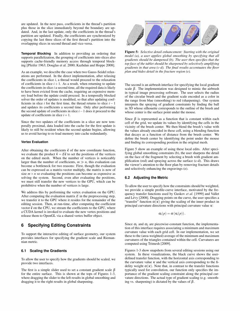
Figure 5: Selective detail enhancement: Starting with the originalmodel (a), a user applies global smoothing by specifying that allgradients should be dampened (b). The user then specifies that thetop face of the tablet should be sharpened by selectively amplifyinggradients in that area (c-d). The final results accentuates the floorplan and hides detail in the fracture region (e).

The second is an airbrush interface for specifying the local gradientscale β . The implementation was designed to mimic the airbrushin typical image processing software. The user selects the radiusof the circular brush and the gradient scale encoded as a color inthe range from blue (smoothing) to red (sharpening). Our systeminterprets the spraying of gradient constraints by finding the ballin 3D whose silhouette corresponds to the outline of the brush andwhose center is the surface point under the mouse.

Since β is represented as a function that is constant within eachcell of the grid, we update its values by identifying the cells in thevicinity of the brush center. We then blend the brush’s value withthe values already encoded in these cell, using a blending functionthat decays as a function of distance from the brush center. Wedefine the brush center by identifying the point under the mouseand finding its corresponding position in the original mesh.

Figure 5 show an example of using these local edits. After speci-fying global smoothing constraints (b), the user sharpens the detailon the face of the fragment by selecting a brush with gradient am-plification (red) and spraying across the surface (c-d). This drawsthe viewer’s attention to the floor plan by removing fracture detailsand selectively enhancing the engravings (e).

6.2 Adjusting the Metric

To allow the user to specify how the constraints should be weighted,we provide a simple profile-curve interface, motivated by the fre-quency transfer functions used by Guskov et al. [1999] and Valletand Levy [2008]. Dragging points on the curve, the user specifies a“transfer” function α(κ) giving the scaling of the inner product inprincipal curvature directions with principal curvature value κ:

αi(p) = α (κi(p)) .

Since α1 and α2 are piecewise-constant function, the implementa-tion of this interface requires associating a minimum and maximumcurvature value with each grid cell. In our implementation, we setthese to the (area-weighted) average of the minimum and maximumcurvatures of the triangles contained within the cell. Curvatures arecomputed using Trimesh [2009].

Figures 1-3 show snapshots from several editing sessions using oursystem. In these visualizations, the black curve shows the user-defined transfer function, with the horizontal axis corresponding tothe curvature value κ and the vertical axis corresponding to the fi-delity weight α(κ). Note that, in contrast to the transfer functionstypically used for convolution, our function only specifies the im-portance of the gradient scaling constraint along the principal cur-vature directions. The actual type of gradient scaling (e.g. smooth-ing vs. sharpening) is dictated by the values of β .

Figure 6: Efficiency (left and center) and accuracy (right) of oursolver: The plots show results for finite-elements systems defined byoctrees at different depths and highlight the contributions of paral-lelization and temporal blocking in different architectures.

7 Evaluation and Discussion

To evaluate our system, we study how accuracy and efficiency areaffected by the different design choices. We begin with an analysisof the solver itself and then look at the system as a whole. Weconclude with a discussion of our method.

7.1 Solver Evaluation

To analyze the performance of our solver outside the context of anediting system, we would like to determine how running time andsolution accuracy behave as functions of (1) problem size, (2) num-ber of iterations, (3) parallelization, and (4) temporal blocking. Forthese experiments, we assume no prior knowledge so we instantiatethe solution to zero and solve using a W-cycle multigrid solver. Weevaluate the accuracy of our solver as the ratio of the norm of theresidual to the norm of the initial constraints.

We run the experiments on two architectures, a desktop with a 2.66GHz Intel Core i7 920 processor and a notebook with a 2.54 GHzIntel Core 2 Extreme Q9300 processor. Both have four cores. Thedesktop shares an 8MB L3 cache between the cores and the note-book splits a 6 MB L2 cache in a two-by-3 MB configuration.

The results of our experiments with the Forma Urbis Romae frag-ment, using double-precision arithmetic, can be seen in Figure 6.

The plots show the running time (left and center) and accuracy(right) of the solvers and compare the performance of serial imple-mentations without temporal blocking (solid line), parallel imple-mentations without temporal blocking (dashed line), and parallelimplementations with temporal blocking (dotted line). The plotsalso compare the performance across systems of different resolu-tions, using a function basis derived from an octree of depth 7 (or-ange), depth 8 (blue), and depth 9 (red), with 7.9×104, 3.2×105,and 1.3×106 leaf nodes at the finest level, respectively. The ac-curacy and running time are given as a function of the number ofW-cycles performed, with five Gauss-Seidel relaxations performedat each level of the multigrid hierarchy.

The results highlight different features of our implementation. Forexperiments run on the desktop, the cache is sufficiently large thatmemory access does not bottleneck the system. As a result, thesolver shows a 200% improvement with parallelization, but only anadditional 5% improvement with temporal blocking. In contrast, onthe cache-constrained notebook, parallelization across four proces-sors only shows a 150% improvement in running time, while theimprovement due to temporal blocking increases to roughly 20%.

In the accuracy plots, we see that the parallelization and tempo-ral blocking give errors that are indistinguishable from the serial,

Figure 7: Efficiency of our interactive solver: The chart shows thecontribution, measured in increased interactivity, gained by per-forming the vertex evaluation on the GPU, leveraging paralleliza-tion, and using temporal blocking at different octree depths, d.

non-blocking solver. This confirms that our system correctly im-plements Gauss-Seidel relaxations and that parallelization and tem-poral blocking do not affect the precision of the solver.

7.2 System Evaluation

In the context of an interactive editing system, we assume that thesolution to the screened Poisson equation in one frame should be agood initial guess for the relaxation in the next. As a result, we usea less aggressive solver, performing a V-cycle to relax the solution,with just two Gauss-Seidel relaxation steps per level.

Since this solver exposes different performance characteristics fromthose exhibited by the stand-alone solver, we re-evaluate the run-ning time as a function of (1) problem size, (2) parallelization, and(3) temporal blocking. Additionally, we look at the performancegains obtained by using the GPU to evaluate the vertex positions.

For these experiments, we use the desktop described above,equipped with an NVIDIA GeForce GTX 260 video card.

The results of these experiments are shown in Figure 7, which givesthe frames-per-second achieved with our solver, for three differ-ent models, using the finite-element systems defined by octrees ofdifferent depths. The charts compare the performance of differentimplementations of the solver, allowing us to explore the benefitsgained by relegating the vertex evaluation to the GPU, paralleliz-ing the solver, and using temporal blocking. As expected, whenthe depth of the octree is low, the solution of the screened Pois-son equation is less computationally expensive than the evaluationof the vertex positions, and using the GPU to evaluate the vertexpositions provides the greatest gains. However, as the depth is in-creased, the solution of the system starts playing a more significantrole, and the contributions of an efficient solver, measured in in-creased frames-per-second, become more apparent.

Frames/Second SolverVertices DoFs Solve RHS Matrix Speed-Up

Lucy 2.6·105 3×1.5·10

5 40 20 8 ×2.7Buddha 5.4·10

5 3×2.1·105 31 15 6 ×2.6

Armadillo 1.7·105 3×2.6·10

5 30 13 5 ×3.3Dragon 4.4·10

5 3×2.7·105 27 12 5 ×3.0

Isidore 1.1·106 3×2.8·10

5 27 12 4 ×3.0Forma 1.0·10

6 3×3.2·105 24 11 4 ×3.0

David 2.0·106 3×4.2·10

5 20 9 3 ×3.3

Table 1: Model summary: Statistics of the geometric complexity,numbers of degrees of freedom, frame-rate, and speed-up due toparallelization and temporal blocking for the models in this work.

A summary of the performance for the different models discussedin this work can be seen in Table 1. The statistic reflect the perfor-mance when the finite-elements system is defined by an octree ofdepth 8 and the speed-up is measured over a non-blocking, serial,single-precision, implementation that performs the vertex evalua-tion on the GPU.

The three running times correspond to the three states of the system:

1. Solve: When the user has not specified any edits, the systemperforms a multigrid solve at each frame and then updates thevertex positions.

2. RHS: When the user modifies the gradient scales, the right-hand-side of the system is computed before solving and up-dating the vertex positions.

3. Matrix: When the user modifies the filter by adjusting themetric, both the system matrices and right-hand-side are com-puted before solving and updating the vertex positions.

As the table shows, our solver exhibits a roughly three-fold im-provement in performance for all of the models and supports inter-active modification of both the gradient scale and the underlyingRiemannian metric for high-resolution models.

Evaluating the accuracy of our interactive solver, we find that evenafter significant modifications to both the gradient scale and thetransfer function, the residual norm drops below 10−4 after just afew frames. In practice this means that we can process models likethe David head, which define a 4× 105-dimensional system, in afraction of a second and obtain an artifact free visualization of ourediting choices. In contrast, the recent solver of Shi et al. [2006]takes almost a second and a half to converge to a residual norm thatis smaller than 10−3 for a 4.1×105-dimensional system.

7.3 Discussion

Smoothness and Aliasing To implement our interactive system,we use an octree-based finite-elements system with first-order B-splines defining the test functions. The use of the octree allowsus to bound the dimensionality of the system independent of thenumber of vertices in the mesh, while the piecewise-tri-linearity ofthe functions reduces their support, resulting in a sparser system.Though our choices enable an efficient solver, the limitations ofthese choices become apparent as the resolution of the octree isreduced to push efficiency to its limit.

An example of the limitations of these choices is visualized in Fig-ure 8, which shows the result of applying gradient dampening to the“Isidore Horse” model. The top row shows the original model, themodel obtained as a result of gradient dampening at depth 8, and aclose-up of the detail on the horse’s head. The middle row showsclose-ups from the results of gradient dampening at different octreedepths, using first-order B-splines.

The figure shows that as the depth of the octree is reduced fromeight, to six, to four, the support of the B-splines is more denselysampled by the vertices in the mesh, revealing the C0 nature of thetest functions. To validate that these visual artifacts are the resultsof the piecewise-linear nature of the first-order B-splines and notaliasing, we re-ran the gradient dampening with second-order el-ements, using an offline solver. As the images in the bottom rowof Figure 8 indicate, the switch to smoother functions successfullyremoves the first-order discontinuity artifacts.

Examining the figures more carefully, we find that the expectedaliasing artifacts do arise at lower depths, though they are moresubtle. They are particularly evident in the results obtained usingan octree of depth four, and are manifest as detail that could not

Figure 8: Limitation of our approach: Due to the use of first-orderB-splines in defining our finite-elements, the piecewise-linear na-ture of the functions becomes apparent when the element resolutionis much coarser than the mesh resolution. Though transitioning tosecond-order B-splines is computationally more expensive, it caneffectively alleviate these limitations by providing C1 continuity.

be smoothed out through gradient dampening, such as the eye, thenostril, and the reigns. Informally, we have found that the alias-ing artifacts become more prevalent as the gradient scale deviatesfrom β = 1, but we are still exploring a more concrete relationshipbetween the resolution of features on the mesh, support-size of theB-splines, magnitude of the gradient scale, and aliasing artifacts.

GPU-Based Implementation In our work, we have chosen topursue a CPU-based implementation of the solver. In the future,we would like to adapt the GPU-based Poisson solver of Zhouet al., designed for surface reconstruction [2010], to our context.One challenge of doing so is that the GPU-based implementationwas designed for solving a (stationary) volumetric Poisson equa-tion. In that context, the value of the IJ-th matrix coefficient onlydepends on the relative position of cells I and J, allowing for thememory-efficient representation of the Laplace operator by a small(3× 3× 3) stencil. In contrast, both the anisotropy of our sys-tem, and the fact that coefficients depend on how the surface passesthrough the grid cells, require the explicit computation and storageof each matrix coefficient.

We also note that though the construction of our linear system isimplemented on the CPU and the system is non-stationary, our per-formance is still within a factor of about three of the performanceof the stationary, GPU-based implementation of Zhou et al. For ex-ample, our method constructs and solves the matrix for a 4.2×105-dimensional system in roughly 0.3 seconds. By comparison, theGPU implementation of Zhou et al. constructs and solves the ma-trix for a 6.7×105-dimensional system in roughly 0.15 seconds.

8 Conclusion

In this work, we have described a general framework for perform-ing curvature-aware geometry filtering through the solution of ascreened Poisson equation. We have shown that the system can beefficiently adapted to a changing Riemannian metric and have de-scribed a parallel and streaming multigrid implementation for solv-ing the system. Combining these, we develop the first interactive

system that supports the exploration of a rich landscape of meshfilters for real-time geometry processing.

Though our presentation has focused on the real-time editing of ge-ometry, our approach can be generalized in a number of ways. Thesystem can easily be adapted to the editing of other per-vertex quan-tities, such as colors and normals. The temporal blocking used tostream through memory can be leveraged to develop an out-of-coresolver. And, the decomposition of coefficients enabling coarse-grained parallelization can be used to develop a distributed solver.

Finally, we would also like to enrich our system by supporting theuse of a palette of profile-curves. This would allow users to applydifferent curvature transfer functions to different parts of the mesh,further expanding the types of filtering operations supported.

References

AKSOYLU, B., KHODAKOVSKY, A., AND SCHRODER, P. 2003.Multilevel solvers for unstructured surface meshes. SIAM Jour-nal of Scientific Computing 26.

BAJAJ, C. L., XU, G. L., BAJAJ, R. L., AND T, G. X. 2002.Anisotropic diffusion of subdivision surfaces and functions onsurfaces. ACM Transactions on Graphics 22, 4–32.

BHAT, P., CURLESS, B., COHEN, M., AND ZITNICK, L. 2008.Fourier analysis of the 2D screened Poisson equation for gra-dient domain problems. In Proceedings of the 10th EuropeanConference on Computer Vision, 114–128.

BHAT, P., ZITNICK, L., COHEN, M., AND CURLESS, B. 2010.Gradientshop: A gradient-domain optimization framework forimage and video filtering. ACM Transactions on Graphics 29,10:1–10:14.

BURT, P., AND ADELSON, E. 1983. The Laplacian pyramid as acompact image code. IEEE Transactions on Communication 31,532–540.

CHUANG, M., LUO, L., BROWN, B., RUSINKIEWICZ, S., ANDKAZHDAN, M. 2009. Estimating the Laplace-Beltrami operatorby restricting 3D functions. Computer Graphics Forum (Sympo-sium on Geometry Processing), 1475–1484.

CLARENZ, U., DIEWALD, U., AND RUMPF, M. 2000. Anisotropicgeometric diffusion in surface processing. Visualization Confer-ence, IEEE 0, 70.

COWPER, C. 1973. Gaussian quadrature formulas for triangles.International Journal of Numerical Methods in Engineering 7,405–408.

DESBRUN, M., MEYER, M., SCHRODER, P., AND BARR, A.1999. Implicit fairing of irregular meshes using diffusion andcurvature flow. In ACM SIGGRAPH Conference Proceedings,317–324.

DOUGLAS, C., HU, J., KOWARSCHIK, M., RUDE, U., ANDWEISS, C. 2000. Cache optimization for structured and un-structured grid multigrid. Electronic Transactions on NumericalAnalysis 10, 21–40.

ECKSTEIN, I., PONS, J.-P., TONG, Y., KUO, C., AND DESBRUN,M. 2007. Generalized surface flows for mesh processing. InSymposium on Geometry Processing, 183–192.

GUSKOV, I., SWELDENS, W., AND SCHRODER, P. 1999. Mul-tiresolution signal processing for meshes. In ACM SIGGRAPHConference Proceedings, 325–334.

KAZHDAN, M., AND HOPPE, H. 2008. Streaming multigrid forgradient-domain operations on large images. ACM Transactionson Graphics (SIGGRAPH ’08) 27.

KOBBELT, L., CAMPAGNA, S., VORSATZ, J., AND SEIDEL, H.1998. Interactive multi-resolution modeling on arbitrary meshes.In ACM SIGGRAPH Conference Proceedings, 105–114.

MCCANN, J., AND POLLARD, N. 2008. Real-time gradient-domain painting. ACM Transactions on Graphics (SIGGRAPH’08) 27.

MEYER, M., DESBRUN, M., SCHRODER, P., AND BARR, A.2002. Discrete differential-geometry operators for triangulated2-manifolds. Visualization and Mathematics 3, 34–57.

OHTAKE, Y., BELYAEV, A., AND BOGAEVSKI, I. 2000. Poly-hedral surface smoothing with simultaneous mesh regulariza-tion. In Proceedings of the Geometric Modeling and Processing(GMP ’00), 229–237.

PFEIFER, C. 1963. Data flow and storage allocation for the PDQ-5 program on the Philco-2000. Communications of the ACM 6,365–366.

PINKALL, U., AND POLTHIER, K. 1993. Computing discrete min-imal surfaces and their conjugates. Experimental Mathematics 2,15–36.

SHI, L., YU, Y., BELL, N., AND FENG, W. 2006. A fast multigridalgorithm for mesh deformation. ACM Transactions on Graphics(SIGGRAPH ’06) 25, 1108–1117.

SMITH, B., BJORSTAD, P., AND GROPP, W. 1996. DomainDecomposition: Parallel Multilevel Methods for Elliptic PartialDifferential Equations. Cambridge University Press.

TASDIZEN, T., WHITAKER, R., BURCHARD, P., AND OSHER, S.2002. Geometric surface smoothing via anisotropic diffusion ofnormals. In VIS ’02: Proceedings of the conference on Visu-alization ’02, IEEE Computer Society, Washington, DC, USA,125–132.

TAUBIN, G. 1995. A signal processing approach to fair surfacedesign. In ACM SIGGRAPH Conference Proceedings, 351–358.

TRIMESH 2.9, 2009.www.cs.princeton.edu/gfx/proj/trimesh2/.

VALLET, B., AND LEVY, B. 2008. Spectral geometry processingwith manifold harmonics. Computer Graphics Forum (Proceed-ings Eurographics) 27, 251–160.

WEBER, O., DEVIR, Y., BRONSTEIN, A., BRONSTEIN, M., ANDKIMMEL, R. 2008. Parallel algorithms for approximation ofdistance maps on parametric surfaces. ACM Transactions onGraphics 27.

WITKIN, A. 1983. Scale-space filtering. In International JointConference on Artificial Intelligence, 1019–1022.

ZHOU, K., GONG, M., HUANG, X., AND GUO, B. 2010. Data-parallel octrees for surface reconstruction. IEEE Transactionson Visualization and Computer Graphics.