Technical report from Automatic Control at Linköpings universitet

Interactive analysis of time-varying sys-tems using volume graphics

Jimmy Johansson, David Lindgren, Matthew Cooper,Lennart LjungDivision of Automatic ControlE-mail: jimjo@itn.liu.se, lindgren@isy.liu.se,matco@itn.liu.se, ljung@isy.liu.se

14th June 2007

Report no.: LiTH-ISY-R-2798Accepted for publication in Proc. Conference on Decision and Control,Bahamas 2004

Address:Department of Electrical EngineeringLinköpings universitetSE-581 83 Linköping, Sweden

WWW: http://www.control.isy.liu.se

AUTOMATIC CONTROLREGLERTEKNIK

LINKÖPINGS UNIVERSITET

Technical reports from the Automatic Control group in Linköping are available fromhttp://www.control.isy.liu.se/publications.

Abstract

We show how 3-dimensional volume graphics can be used as a tool in

system identi�cation. Time-dependent dynamics often leave a signi�cant

residual with linear, time-invariant models. The structure of this residual is

decisive for the subsequent modelling, and by using advanced visualization

techniques, the modeller may gain a deeper insight into this structure than

that which can be obtained by standard correlation analysis. We present

a development platform that merges a rich variety of estimation programs

with state of the art visualization techniques.

Keywords: identi�cation

Interactive Analysis of Time-Varying Systems usingVolume Graphics

Jimmy Johansson, David Lindgren, Matthew Cooper and Lennart Ljung

Abstract— We show how 3-dimensional volume graphics canbe used as a tool in system identification. Time-dependentdynamics often leave a significant residual with linear, time-invariant models. The structure of this residual is decisive forthe subsequent modelling, and by using advanced visualizationtechniques, the modeller may gain a deeper insight into thisstructure than that which can be obtained from standardcorrelation analysis. We present a development platform thatmerges a rich variety of estimation programs with state of theart visualization techniques.

I. I NTRODUCTION

A. Interaction in System Identification

System Identification is inherently an interactive art.Results from preliminary model building are studied bythe user. Based on such studies, decision about new modelstructures are taken. The studies are typically of visualnature, often simple 2-dimensional line plots of correlationfunctions and residuals. Visualization techniques have gonethrough a significant development during the past decade. Itis an interesting problem to study what such new techniquesmay offer in terms of improved interaction in systemidentification. The purpose of the present contribution isto give some illustrations of what can be achieved in thisway. No new identification methods and no new modelindicators will be introduced, but new ways to visualize theinformation in a suggestive manner. The study is a resultbetween a research group in system identification and onein scientific visualization.

B. Time Invariant Models and Time-varying Systems

Fitting a time-invariant model to data sampled from asystem with time-varying dynamics is, of course, possiblebut often results in a large-magnitude time-varying residual.Unless we are aware from the beginning of the time-variantnature of the system dynamics the cause of the large residualmagnitude will, perhaps, not be evident. Covariation andauto-covariation estimates reveal that something is wrongbut give no clue to whether the bad fit is due to wrongmodel order, non-linearities or time-variant dynamics. Atthis point, it is actuallydifficult to gain insight into themodel discrepancies. Volume graphics in 3 dimensions,however, offers a means to go beyond standard summarystatistics measures for model validation. By assigning each

Jimmy Johansson,jimjo@itn.liu.se , and Matthew Cooper,matco@itn.liu.se , are with the Department of Science and Tech-nology, Linkoping University, Sweden

David Lindgren, david@isy.liu.se , and Lennart Ljung,ljung@isy.liu.se , are with the Division of Automatic Control,Linkoping University, Sweden

data point to a semi-transparent volume in a 3-dimensionalspatial/temporal space, the modeller may explore and inter-pret large-scale process data sets (104-105 sample points).

The process ofsystem identification[9] can be brokendown into 3 steps:

1) Select model structure.2) Estimate model parameters given data sampled from

a system and generate the model residual – the partof the output that is left unmodelled.

3) Validate the model. If the residual issatisfactorythen finish, else select another model structure andstart again. A satisfactory residual is, for instance, aresidual small in magnitude and independent of themodel/system input.

In this work we show how step 3 above can be aided bythe use of interactive 3-dimensional volume graphics, inparticular, how time-varying dynamics and other potentialinadequacies of the model can be effectively detected.

Being able to visualize data with multiple visualiza-tion techniques in multiple views can be powerful whenanalysing complex data. There exist a large number ofvisualization techniques for 2- and 3-dimensional data.One of the simplest and most widely used techniques isthe 2-dimensional scatter plot which simply shows therelationship between two variables (Fig. 1). A more sophis-ticated way of visualizing data is to use a volume graphicstechnique [4]. Volume graphics is used for visualizingsampled functions of three spatial dimensions by computing2-dimensional projections of a coloured, semitransparentvolume. One common application area of volume graphicsis in the medical imaging domain where, for example, datacan be constructed from the output of an X-ray ComputedTomography (CT) scanner. However, visualization alone isusually not enough in order to fully understand the data.Of equal importance are also correct pre-processing of thedata and the ability to interact and manipulate with theresult. Using linked views [11], [14] is one technique, whichenables the investigation of the same data in several views atthe same time. This facilitates the discovery of unexpectedrelationships since multiple views are used. With linkedviews, a movement in one view is automatically propagatedto all other views. In combination with different zoomlevels, a setup of two or three linked views is useful tocreate a focus-plus-context [3] configuration. Many othercombinations are possible where linked views reduce theuser’s cognitive load compared to the case of two indepen-dent views.

−3 −2 −1 0 1 2 3−1

−0.5

0

0.5

1

1.5

2

ut

et

Fig. 1. A simple scatter plot showing samples from two dependent butuncorrelated random variables.

C. Related Work

The visualization and estimation techniques we use inthis work are well-known in their respective disciplines.Using volume graphics as an interactive tool for systemidentification, however, we have not seen elsewhere. Whatwe have seen, though, are great efforts being made tovisualize complex process data, for instance, by means ofscatter plot matrices and parallel coordinates, [5], [7] Theapplications have mainly been for decision support, see [8].For an overview of concepts and taxonomies of visual dataexploration, see [2].

II. M ODEL VALIDATION

We will use a linear discrete time-invariant state spacemodel {

xt+1 = Axt +But

yt = Cxt .(1)

Here, ut is the input signal (common to the system andmodel), yt the simulated model output andyt the sampledoutput signal of the system to be identified. The modelordern is the same as the dimensionality of the state spacevector xt . Given n (design parameter), a set{ut ,yt}N

1 withsampled data points and some assumption of the initialstatex0, techniques to estimate the model parametersA,B,Care well-known (state-space subspace system identification),see [12]. Programs for this task are available commercially,for instance theSystem Identification Toolbox[10] for usewith MATLAB.

Once the model parameters are estimated and ˆy simulatedaccording to (1), the model residual is calculated as

et = yt − yt , t = 1,2, . . . ,N. (2)

If the model is a correct description of the sampled system,the residual will depend only on some unknown noiseprocess, not on the input. In fact, if the residual is inde-pendent of present and past inputs, nothing more is left to

+

−

Model

Residual, e

Noise

t

t

t

System output, y

Model output, y

Input, ut System(discrete)

Fig. 2. Model validation. The outputyt of the system, here discrete, iscompared to the output of the model, ˆyt . The difference between the twomakes the residual,et . If the residual is dependent on the noise only, noton the inputut , then there is nothing more to model.

be modelled and the process is complete. Fig. 2. illustratesthe signal paths.

A standard measure of the dependence between twoscalar, zero-mean samples is the sample cross covariance,

Reu(τ) =1

N− τ

N−τ

∑t=1

et+τut . (3)

If some Reu(τ) is significantly larger than 0, this indicatesthe model is not sufficient. Plotting{et} against{ut+τ} indifferent 2-dimensional scatter plots forτ = 0,1, . . . mayhowever reveal dependencies not reflected byReu at all.Fig. 1 illustrates this by plotting samples from two evidentlydependent random variables that are totally uncorrelated,Reu(0) = 0. To also visualizetime-varyingdependencies itwill be necessary to use 3-dimensional graphics to displayet+τ , ut , and t. This gives rise to a number of issues wewill address in the subsequent sections.

III. I MPLEMENTATION

Our software platform exploits the system identificationtoolbox in MATLAB together with a powerful object-oriented visualization system, AVS/Express [1]. This systemis based on individual modules and an application is built bycombining these through a visual network editor. MATLABand AVS/Express have been seamlessly integrated througha common user interface with which the user can inter-actively pre-process, analyse and visualize their data. Ourapplication has also been extended from an ordinary desktopPC to a much larger semi-immersive stereoscopic display.This type of visualization creates the psychological illusionof being inside the computer-generated environment, ratherthan viewing it from the outside through a screen. The usercan interact with the visualization to navigate through andcontrol the positions of the objects. Stereoscopic visionseems to be specially promising when analysing largecomplex data.

A. Application Overview

A simplified work flow of our application is shown inFig. 3. The work flow begins with loading data from a

file into MATLABs workspace. The user can choose tovisualize the original data set but can also perform a numberof pre-processing operations on the data. The next stepin the analysis process is to choose an appropriate modelstructure and to perform the estimation. Through the userinterface, the user can look at a preview of the estimationresult in a 2-dimensional scatter plot. This process is highlyinteractive so the user can at any time go back and changethe parameters of the model to further improve the resultof the visualization. When the user has identified an areaof interest, it can be visualized using a volume graphicstechnique. In Fig. 4 this is illustrated on data from a sampledfeed-back system where the closed loop gain is increasedat the end of the sequence. The axes aret, et and ut−1.To further investigate the data, linked views can be used toanalyse a cross-section of the data.

To manage the communication between MATLAB andAVS/Express, we have developed a communication module.This module handles all control messages and the entireflow of data between the two systems. Since system iden-tification data may be large, the data is (as far as possible)handled locally by MATLAB. It is only when the userexplicitly requests data that it is transferred from MATLABto AVS/Express. Also, it is only the selected subset thatis sent, never the entire data set. This makes the process-ing of large data sets much easier and the visualizationprocess highly interactive. Our module can be used in allAVS/Express applications and can be downloaded for freefrom the International AVS Centre [6].

Estimate model

MatlabAVS/Express

Browse for data

Calculate data statistics

Pre−process data

Choose model

Visualize data Data

Specify parameters

Read data from file

Flow of data

Control messages

Steps in the analysis process

Fig. 3. The work flow between AVS/Express and MATLAB.

B. Interactive Volume Graphics

In the analysis process it is possible to perform a volumegraphics visualization of a selection of variables. This 3-dimensional visualization technique effectively reveals anytime-variations and is an important part of the analysis

process (Fig. 5). To some extent it can also be used toidentify non-linear dependencies but more work needs tobe done to systemise the process.

To make the volume graphics visualization interactive weneed to re-calculate the volume data every time the usermakes a change in the parameter settings. How quickly thiscan be done primarily depends on the volume size and onthe type of platform used. The calculation, described below,and rendering of the visualization of a 128× 128× 256volume on a desktop PC can be done with only one or twoseconds of delay. The size of the volume can dynamicallybe changed to speed up the calculations on a slower PC. Toconstruct the volume data we extract a subsetd of the 2-dimensional data (Fig. 6). Each plane in the volume consistsof an n×m matrix of bins and the data points, scaled by asuitable factor in each dimension, are aggregated into thesebins as a simple population count. The scaling factors arecalculated so that{

xscaledi = m

max(~x)xi

yscaledi = n

max(~y)yi .(4)

This procedure is done for every subset, which gives usa volume of sizem×n× t

d .

x y

n

m

time (t)

time (t)

d

d

d

Fig. 6. A subset of the 2-dimensional data is scaled and aggregated. Thisis done for every subsetd, which gives a volume of sizen×m× t

d .

C. Application Performance and Timing

To perform a complete analysis of a data set, a numberof visualization modules and MATLAB libraries are used.We have identified the model estimation to be the mosttime consuming operation in our application. The time forestimating a third order linear state-space model of a dataset with 40,000 observations may be ten times as long asloading the data, which is the second most time consumingoperation.

We have conducted a series of performance tests onour model estimation library. These tests were done on aPC running Windows XP with an Intel Pentium 4 CPU(2.40 GHz) with 256 MB RAM. As test data we used atime-varying data set where we used one input and oneoutput variable, with a growing number of observations.The results are presented in Fig. 7, where we can see that

Fig. 4. Six different view angles of time-varying data visualized using a 3-dimensional volume graphics technique.

Fig. 5. Our application running on a semi-immersive display. The 2-dimensional scatter plot in the upper left view shows the relationship betweenutandet . From the visualization we can clearly see that there is a correlation, which implies that there are still information left to be described. There isalso another region, which is less correlated and the problem is that the 2D scatter plot gives no information about where in time these separate regionsare. Visualizing the same variables with a volume graphics technique (right view) gives the necessary temporal information. To further investigate therelationship between these variables, the cross-section from the clip plane is displayed in the lower left view. The plane can also be animated throughthe entire time sequence.

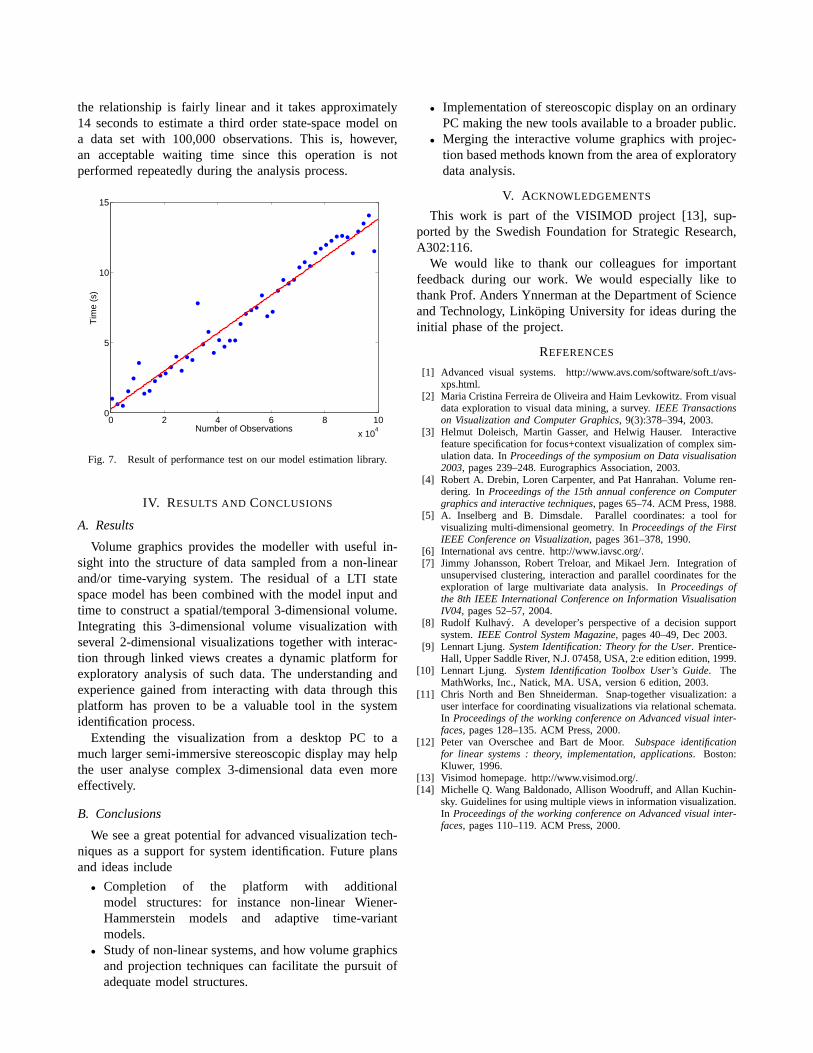
the relationship is fairly linear and it takes approximately14 seconds to estimate a third order state-space model ona data set with 100,000 observations. This is, however,an acceptable waiting time since this operation is notperformed repeatedly during the analysis process.

0 2 4 6 8 10

x 104

0

5

10

15

Number of Observations

Tim

e (s

)

Fig. 7. Result of performance test on our model estimation library.

IV. RESULTS AND CONCLUSIONS

A. Results

Volume graphics provides the modeller with useful in-sight into the structure of data sampled from a non-linearand/or time-varying system. The residual of a LTI statespace model has been combined with the model input andtime to construct a spatial/temporal 3-dimensional volume.Integrating this 3-dimensional volume visualization withseveral 2-dimensional visualizations together with interac-tion through linked views creates a dynamic platform forexploratory analysis of such data. The understanding andexperience gained from interacting with data through thisplatform has proven to be a valuable tool in the systemidentification process.

Extending the visualization from a desktop PC to amuch larger semi-immersive stereoscopic display may helpthe user analyse complex 3-dimensional data even moreeffectively.

B. Conclusions

We see a great potential for advanced visualization tech-niques as a support for system identification. Future plansand ideas include

• Completion of the platform with additionalmodel structures: for instance non-linear Wiener-Hammerstein models and adaptive time-variantmodels.

• Study of non-linear systems, and how volume graphicsand projection techniques can facilitate the pursuit ofadequate model structures.

• Implementation of stereoscopic display on an ordinaryPC making the new tools available to a broader public.

• Merging the interactive volume graphics with projec-tion based methods known from the area of exploratorydata analysis.

V. ACKNOWLEDGEMENTS

This work is part of the VISIMOD project [13], sup-ported by the Swedish Foundation for Strategic Research,A302:116.

We would like to thank our colleagues for importantfeedback during our work. We would especially like tothank Prof. Anders Ynnerman at the Department of Scienceand Technology, Linkoping University for ideas during theinitial phase of the project.

REFERENCES

[1] Advanced visual systems. http://www.avs.com/software/softt/avs-xps.html.

[2] Maria Cristina Ferreira de Oliveira and Haim Levkowitz. From visualdata exploration to visual data mining, a survey.IEEE Transactionson Visualization and Computer Graphics, 9(3):378–394, 2003.

[3] Helmut Doleisch, Martin Gasser, and Helwig Hauser. Interactivefeature specification for focus+context visualization of complex sim-ulation data. InProceedings of the symposium on Data visualisation2003, pages 239–248. Eurographics Association, 2003.

[4] Robert A. Drebin, Loren Carpenter, and Pat Hanrahan. Volume ren-dering. InProceedings of the 15th annual conference on Computergraphics and interactive techniques, pages 65–74. ACM Press, 1988.

[5] A. Inselberg and B. Dimsdale. Parallel coordinates: a tool forvisualizing multi-dimensional geometry. InProceedings of the FirstIEEE Conference on Visualization, pages 361–378, 1990.

[6] International avs centre. http://www.iavsc.org/.[7] Jimmy Johansson, Robert Treloar, and Mikael Jern. Integration of

unsupervised clustering, interaction and parallel coordinates for theexploration of large multivariate data analysis. InProceedings ofthe 8th IEEE International Conference on Information VisualisationIV04, pages 52–57, 2004.

[8] Rudolf Kulhavy. A developer’s perspective of a decision supportsystem.IEEE Control System Magazine, pages 40–49, Dec 2003.

[9] Lennart Ljung.System Identification: Theory for the User. Prentice-Hall, Upper Saddle River, N.J. 07458, USA, 2:e edition edition, 1999.

[10] Lennart Ljung. System Identification Toolbox User’s Guide. TheMathWorks, Inc., Natick, MA. USA, version 6 edition, 2003.

[11] Chris North and Ben Shneiderman. Snap-together visualization: auser interface for coordinating visualizations via relational schemata.In Proceedings of the working conference on Advanced visual inter-faces, pages 128–135. ACM Press, 2000.

[12] Peter van Overschee and Bart de Moor.Subspace identificationfor linear systems : theory, implementation, applications. Boston:Kluwer, 1996.

[13] Visimod homepage. http://www.visimod.org/.[14] Michelle Q. Wang Baldonado, Allison Woodruff, and Allan Kuchin-

sky. Guidelines for using multiple views in information visualization.In Proceedings of the working conference on Advanced visual inter-faces, pages 110–119. ACM Press, 2000.

Avdelning, Institution

Division, Department

Division of Automatic ControlDepartment of Electrical Engineering

Datum

Date

2007-06-14

Språk

Language

� Svenska/Swedish

� Engelska/English

�

�

Rapporttyp

Report category

� Licentiatavhandling

� Examensarbete

� C-uppsats

� D-uppsats

� Övrig rapport

�

�

URL för elektronisk version

http://www.control.isy.liu.se

ISBN

�

ISRN

�

Serietitel och serienummer

Title of series, numberingISSN

1400-3902

LiTH-ISY-R-2798

Titel

TitleInteractive analysis of time-varying systems using volume graphics

Författare

AuthorJimmy Johansson, David Lindgren, Matthew Cooper, Lennart Ljung

Sammanfattning

Abstract

We show how 3-dimensional volume graphics can be used as a tool in system identi�cation.Time-dependent dynamics often leave a signi�cant residual with linear, time-invariant mod-els. The structure of this residual is decisive for the subsequent modelling, and by usingadvanced visualization techniques, the modeller may gain a deeper insight into this structurethan that which can be obtained by standard correlation analysis. We present a developmentplatform that merges a rich variety of estimation programs with state of the art visualizationtechniques.

Nyckelord

Keywords identi�cation