Technical Report SL-94- 15I ~july94

AD-A283 088US Army Corpsof EngineersWaterways ExperimentStation

A Model for Assessment of DynamicInteraction Between Magnetically LevitatedVehicles and Their Supporting Guideways

by James C. Ray, Mostafiz R. Chowdhury

"% 94-25150

"ELECTE

Approved For Public Release; Distribution Is Unlimited

DTXC QtTAu r V94 8Prepared for Headquarters, U.S. Army Corps of Engineers

National Maglev Initiativeand U.S. Army Engineer Division, Huntsville

The contents of this report are not to be used for advertising,publication, or promotional purposes. Citation of trade namesdoes not constitute an official endorsement or approval of the useof such commercial products.

A

O F3DfIIDON RUYN PAIUt

Technical Report SL-94-15July 1994

A Model for Assessment of DynamicInteraction Between Magnetically LevitatedVehicles and Their Supporting Guidewaysby James C. Ray, Mostafiz R. Chowdhury

U.S. Army Corps of EngineersWaterways Experiment Station3909 Halls Ferry RoadVicksburg, MS 39180-6199

Final reportApproved for public release; distribution is unlimited

Prepared for Headquarters, U.S. Army Corps of EngineersWashington, DC 20314-1000

National Maglev InitiativeWashington, DC 20590

and U.S. Army Engineer Division, Huntsville

Huntsville, AL 35805

UWder Project E8691 R003, Task 5

US Army Corpsof EngineersWaterways Experimentt"g n" DataStation - i

Ray, James C.

LAOATOM AI• r'O

,IlDOIMOR LAN NAIM TO.I~ l

A model for assessment of dynamic interaction between magneticallylevitated vehicles and their supporting guldeways I by James C. Ray,Mostafiz R. Chowdhury; prepared for Headquarters, U.S. Army Corps ofEngineers, National Maglev Initiative, and U.S. Army Engineer Division,Huntsville.

73 p. : ill. ; 28 cm. - (Technical report ; SL-94-1 5)Includes bibliographic references.1 . Magnetic levitation vehicles. 2. High speed ground transportation -

Design and construction. I. Chowdhury, Mostafiz R. I1. United States.Army. Corps of Engineers. Il1. United States. Army. Corps of Engineers.Huntsville Division. IV. National Maglev Initiative. V. Structures Labora-tory (U.S.) VI. U.S. Army Engineer Waterways Experiment Station. VII.Title. VIII. Series: Technical report (U.S. Army Engineer Waterways Ex-periment Station) ; SL-94-15.TA7 W34 no.SL-94-15

POAE

DTIC T,;•t !

Contents

I--cuctioo ......................................... I

c ow .................. ..................... 3.Objective ........................................... . 2sU ope .. . . . . . .. . . . . . . . . . . . . . . . 3

2- VGI Model ......................................... 5

Model Description .................................... 5Vehicle Ride Quality Analysis Code (RQAC) ................. 9Guideway Analysis Code (GAC) .......................... 14

Genemal ......................................... 14FE mesh creation ................................ 15Modal analysis .................................... 17Strctural analysis ................................ 18

Solution Verification ................................... 22Limitations of VOl Model ............................... 23

Coupled~incoupled* natural frequencies.................... 23Guideway modal contribution............................ 27Multispan analyses ................................. 28

3-VG1 Model Verification ................................ 29

Appromach ........................................... 29Closd-form Solution .................................. 30Finite Element Analysis .............................. 32VGI Model ...................................... 33Results ............................................ 34

4-VGI Model Application ................................. 41

Introduction ......................................... 41FE Mesh Creation .................................. 43Modal Analysis ...................................... 47

Iil

Vehicular Loads ...................................... 52

Structural Analysis .................................... 52

5-Conclusions and Recommendations ........................ 55

Conclusions ......................................... 55Recommendations ..................................... 56

References ............................................ 57

Appendix A: FORTRAN Source Code for Use of DLOAD .......... 59

Appendix B: ABAQUS Input Files ........................... 65

SF298

List of Figures

Figue l. Pictorial of VGl model ........................... 6

Figure 2. Flowchart of VOI model .......................... 8

Figure 3. General vehicle-guideway interaction solution ............ 9

Figure 4. Simplified maglev system .......................... 10

Figure 5. Minimal mesh to represent a simple beam .............. 16

Figure 6. Demonstration of DLOAD subroutine ................. 20

Figure 7. Vehicle definition method for DLOAD subroutine ........ 21

Figure 8. Ordering of foree columns and definitions of the variable"NORMAL" for the DLOAD subroutine ............... 22

Figure 9. Simplified vehicle/guideway model ................... 24

Figure 10. Shift in natural frequencies with relative guideway stiffness .. 25

Figure I1. Influence of vehicle position on coupled frequencies ....... 26

Figure 12. Simplified maglev system ......................... 29

Figure 13. Free-body diagram for the system .................... 30

Iv

Figure 14. Finite element models ............................ 33

Figure 15. Comparison of analytical methods ................... 34

Figure 16. System response for passage speed of 140 mps ........... 35

Figure 17. Vehicle displacement as a function of velocity ........... 36

Figure 18. Bogie displacement as a function of velocity ............ 37

Figure 19. Midspan guideway deflections ...................... 37

Figure 20. Variation of bogie loads with vehicle velocity ........... 39

Figure 21. Foster-Miller maglev system concept .................. 42

Figure 22. Foster-Miller guideway concept ..................... 43

Figure 23. First six bending modes for a two-span continuous beam .... 44

Figure 24. Foster-Miller SCD vehicle ......................... 45

Figure 25. Finite element mesh of Foster-Miller guideway ........... 46

Figure 26. Mode shapes for Foster-Miller guideway ............... 48

Figure 27. Midspan displacements for spans I and 2 of Foster-Millerguideway .................................. . 53

List of Tables

Table 1. Maglev System Parameters ......................... 27

V

Preface

The research reported herein was sponsored by the National MaglevInitiative, Washington. DC, through the U.S. Army Engineer Division,Huntsville, under Project E8691R003. Task 5. Mr. Rick Suever was theProgram Monitor.

All work was carried out by Mr. James C. Ray and Dr. Mostafiz R.Chowdhury, Structural Mechanics Divison (SMD), Structures Laboratory (SL),U.S. Army Engineer Waterways Experiment Station (WES), under the generalsupervision of Mr. Bryant Mather, Director, SL; Mr. J. T. Ballard, AssistantDirector, and Dr. Jimmy P. Balsara, Chief, SMD. The work was conductedduring the period January-December 1993 under the direct supervision ofMr. Ray.

At the time of publication of this report, Director of WES was Dr. RobertW. Whalin. Commander was COL Bruce KL Howard, EN.

M mow a jp m rww am semt t be Medfor eAwtge-. pwblkwd.,or p euduuu pu9wpa CImdwa of &a* maws dml. ao cmaMwl m

".jca uaueusmt or 4s~WlOW fr *W oft eSieh Co~Merdal PA7duc

vi

L -

1 Introduction

Background

Practical superconducting magnetic levitation (Maglev) was firstinvented in the United States in the 1960s. Development of this concept waspursued for a short time in the United States, but in the 1970s, federal fundingwas cut and thus development in the United States effectively ceased. Foreigngovernments however continued development and today, both Germany andJapan have working prototypes.

As a result of the evolving foreign technology and increasingtransportation needs, the United State's interest in Maglev was renewed in1990. In December 1990, the National Maglev Initiative (NMI) was formed bythe Department of Transportation, the Corps of Engineers, and the Departmentof Energy. Its purpose was to continue the analyses conducted earlier inevaluating the potential for Maglev to improve intercity transportation in theUnited States and to determine the appropriate role for the Federal Governmentin advancing this technology.

As part of its evaluation, the NMI sought industry's perspective on thebest ways to implement Maglev technology. They awarded four SystemConcept Definition (SCD) contracts to teams led by Bechtel Corp., Foster-Miller, Inc., Grumman Aerospace Corp., and Magneplane International, Inc..These contracts resulted in very thorough descriptions and analyses of fourinnovative Maglev concepts.

The NMI also formed an independent Government Maglev SystemAssessment (GMSA) team. This team consisted of scientists and engineersfrom the U.S. Army Corps of Engineers (USACE), the U.S. Department ofTransportation (USDOT), and Argonne National Laboratory (ANL), pluscontracted transportation specialists. The team assessed the technical viabilityof the four SCD concepts, the German TRO7 Maglev design, and the FrenchTGV high-speed train (Lever, 1993). Part of these assessments included theuse of existing analytical tools to study and compare various high-risk or high-cost concerns related to each system, such as the guideway structures,magnetic suspensions and stray magnetic fields, motor and power systems, andvehicle/guideway interaction. As a result of these assessments, shortcomingswere recognized in the state-of-the-art of available analytical tools for thispurpose. To address these shortcomings, the NMI funded several

. . .--- m I h h al Imn

projects to further develop specific analytical tools for use in future evaluationsof Maglev designs. The development of the vehicle/guideway interaction(VGI) model reported herein was part of that effort.

VGI refers to the dynamic interaction (coupling) between two separatedynamic systems, the Maglev vehicle and its supporting flexible guideway.The vehicle motion is caused by the roughness and flexibility of its supportingguideway; and the guideway motion is caused by the passage of the vehicle andits time varying suspension forces. In order to accurately predict theperformance of either the vehicle or the guideway, the dynamic interactionbetween the two must be considered.

As a result of previous work related to Maglev, the VNTSC alreadyhad a basic computer model for the assessment of vehicular ride quality overflexible and rough guideways. The model was considered "basic" because itonly allowed two degrees of freedom for the vehicle: pitch and bounce. It wasused successfully in the report by Lever (1993) to perform ride qualityassessments.

Also as a result of previous Maglev work (Lever, 1993), the U.S.Army Engineer Waterways Experiment Station (WES) had determined that theABAQUS Finite Element (FE) program offered the greatest degree offlexibility and accuracy for the dynamic analyses of the diverse range ofpossible Maglev guideway designs. This program was used successfully in thereport by Lever (1993) to perform both two- and three-dimensional static anddynamic guideway analyses.

As seen above, previous work had shown that the analytical capabilityexisted to successfully perform both vehicular ride quality analyses andguideway structural analyses. However, these analyses were completelyindependent of each other and thus a truly coupled analysis between the vehicleand guideway was not accomplished. The work reported herein describes thedevelopment of a model, which intimately links these two analysis procedurestogether and provides a true VGI analysis.

The model has two distinct applications: It can be used to accuratelypredict the vehicle ride quality to be expected from a given vehicle andguideway design; and to accurately predict the dynamic deflections and stressesexperienced throughout the guideway structure as a result of a vehicle passage.Ride quality results are necessary to design a vehicle suspension system and todetermine the guideway stiffness required to meet specific ride quality criteria.Dynamic structural analyses are necessary to produce safe, economical andaccurate guideway designs.

Objective

The objective of this work was to develop a methodology (referred toherein as a "model") for the assessment of the dynamic interaction betweenMaglev vehicles and their supporting guideways. This model will be used topredict the ride quality and stability of Maglev vehicle/guideway designs andthe dynamic response of the guideway as a result of vehicle passage,

2 C8pW 1 In#rouc•m

Scope

The first portion of the project involved the development of a model

for the coupling of two separate analytical processes: one for vehicle ridequality analyses and one for dynamic structural analysis. Once the model wasdeveloped, efforts were focused on improvement and refinement of the existinganalytical processes and verification of the validity and accuracy of the model.The following paragraphs describe these efforts:

The existing vehicle analysis programs only accounted for vehicularpitch and bounce in the vertical plane. These programs were modified to alsoinclude roll, yaw, and lateral sway. All work in this area was accomplished bythe VNTSC. Therefore, only an overview of this portion of the model isprovided herein. A detailed report of this work can be obtained through theVNTSC.

A computer program was written to convert time-varying vehicle bogieforces (determined in the vehicle analysis) into time- and spatially-varyingforces on the FE model of the guideway. This program provided the intimatelink between the vehicle and guideway analytical processes.

The accuracy and validity of the model were verified with a series ofcomparative analyses of a simplified system. The system consisted of a singlemass (representing the vehicle) suspended by both a primary and secondarysuspension (linear springs), which are separated by an intermediate mass(which represents a bogie). This "vehicle' -was moved across the flexible beam(representing the guideway) at various speeds. The response of this systemwas determined and compared using three different solution methods: the VGImodel developed herein, a Closed-form analytical solution, and a FiniteElement analytical solution. In addition to the verification of the VGI model,the model was used to conduct a series of basic parameter studies on thissimplified system. These results were used to study and demonstrate somebasic concepts which are important to the design of a Maglev system.

SFor the purpose of demonstration, the VGI model was applied to theFoster-Miller SCD. This analysis is presented in a step-by-step manner todemonstrate the usage of the VGI Model.

Ctmqt I noducWn 3

2 VGI Model

Model Description

VGI analysis involves the solution of two completely separate andequally complex dynamic systems: the vehicle with its unique 3-dimensionalsuspension and control characteristics; and the guideway with its unique 3-dimensional flexibility characteristics. Since the capabilities existed for each ofthese analyses separately (the vehicle with VNTSC and the guideway withWES), initial consideration was given to the combination of these analyses intoa singular all-in-one VGI model. However, this was found to be impracticaldue to the enormity of each of the calculational processes and the fact that asingular model would severely limit its required flexibility to address allpossible Maglev system designs. Therefore, a "VGI Model" was developedwhich intimately coupled the VNTSC Ride Quality Analysis Code (RQAC) tothe WES Guideway Analysis Code (GAC). The function of the VGI Model isdepicted in the Figure 1. It is also depicted in flowchart form in Figure 2.

Referring to Figures I and 2, the first step in the Model is to build theFE mesh of the guideway (consisting of nodes, elements, and boundaryconditions) and perform a modal analysis with the GAC to determine itsdynamic tnoote shapes and frequencies. These guideway properties are used bythe RQAC to account for the guideway flexibility in the ride quality analysis(Step 2 in the Model). In addition to vehicular accelerations (used for the ridequality assessment), the RQAC also provides a summary of the time variationin bogie forces at the guideway level as a result of passage over the flexibleand randomly-rough guideway. These force-time histories are used to load theFE mesh of the guideway to obtain dynamic deflections and stresses for theguideway (Step 4). Thus, the complete circle is made and the dynamicinteraction between the vehicle and guideway is accounted for in both analyses.The loop is "closed" (i.e. checked for accuracy) in Step 5. The guidewaydeflections predicted by the guideway equation in the RQAC are compared tothose obtained from the GAC. If they do not compare to within reasonablelimits (+/- 15 percent), the process must be repeated using more guidewaymode shapes in the RQAC. The following sections describe in greater detailthe components of the VGI Model and the methods used to link them together.

Ompler 2 VOl Modal 5

0

CL

E

00

X-6-

OW 2 0G O

ii d i ui:n IL

a tif

CWWm 2 VOI Mode7l

S . a a Iii • II I I I

0

0C.

UlU)

.0 0IIItozE

so o

01L

. 0

8 ~ChqdIsr 2 VGI Mo"e

Vehicle Ride Quality Analysis Code (RQAC)

All work on the RQAC was accomplished by the VNTSC. Therefore,only an overview of this portion of the model is provided in the followingparagraphs. A detailed report of the work accomplished on the RQAC can beobtained through the VNTSC.

Figure 3 shows the general vehicle-suspension-guideway interactionproblem. As the vehicle moves along the guideway, it is acted upon byexternal forces and by the suspension system forces which cause linear androtational accelerations of the vehicle. If the vehicle has appreciableflexibility, the forces may also cause significant deformation of the vehiclebody. The suspensions react to the vehicle body and guideway surfacemotions, where the latter include geometric irregularities, intentional camber,and elastic deformations, and produce suspension forces acting on the vehicleand on the guideway. The guideway beams deflect dynamically in response tothe moving, unsteady suspension forces and the reaction forces and momentsgenerated at the support. Finally, the support motions are determined by thesupport and foundation dynamic characteristics and the guideway beam forcesand moments. This strongly coupled situation is extremely complicated ingeneral and simplifying assumptions must be made in order to makeengineering analysis feasible.

EMMAl Guideway

Forces IrrgularityS~+ Camber

Metld Mool • Ve e Foce Gfdde"My

Or le Forces Suspension Dynamics.

and SailDynamics

Figure 3. General vehicle-guideway interaction solution

chapier 2 VGl ModM 9

Figure 4 shows a simplified model which has been employed widely inthe literature for vehicle-guideway dynamic analysis (Richardson and Wormely1974). For this model, only motions in the vertical plane are considered andthe vehicle is assumed to have a rigid body with mass mv and moment ofinertia J about its center of mass. The front and rear suspensions each includea primary suspension (composed of a spring, kp, and damper, cp) which actsdirectly against the guideway, and a secondary suspension consisting of aspring, ks, and damper, cs, or including active elements. A bogie with mass,mb, separates the primary and secondary suspensions.

---- X = Vt--- - .•..- r-- .. , • If - -

.....-• , .... . .... ..

kp' LpCS k , kp f

Figure4. Simplified Maglev system

The governing equations for the vehicle are:

F, 2 { '.+ : It, m-- S 21, (Y J ,

(I)

10 cp2 vG Mode

ow

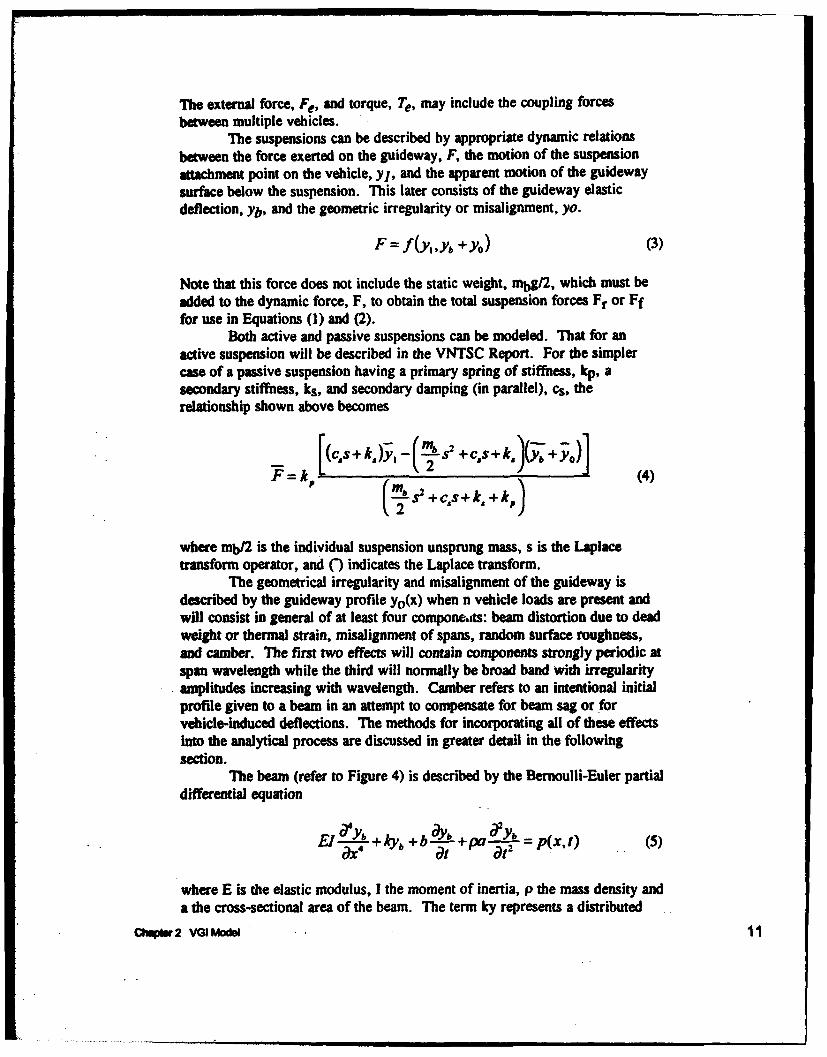
The external force, Fe, and torque, Te, may include the coupling forcesbetween multiple vehicles.

The suspensions can be described by appropriate dynamic relationsbetween the force exerted on the guideway, F, the motion of the suspensionattachment point on the vehicle, yl, and the apparent motion of the guidewaysurface below the suspension. This later consists of the guideway elasticdeflection, Yb, and the geometric irregularity or misalignment, yo.

F = f(y0,yb + yo) (3)

Note that this force does not include the static weight, mbg/2, which must beadded to the dynamic force, F, to obtain the total suspension forces Fr or Fffor use in Equations (1) and (2).

Both active and passive suspensions can be modeled. That for anactive suspension will be described in the VNTSC Report. For the simplercase of a passive suspension having a primary spring of stiffness, kp, asecondary stiffness, ks, and secondary damping (in parallel), cs, therelationship shown above becomes

-(2 S2 +cs+k] (4)( -s2 +c~s+k, +k,)

where mbI2 is the individual suspension unsprung mass, s is the Laplacetransform operator, and ') indicates the Laplace transform.

The geometrical irregularity and misalignment of the guideway isdescribed by the guideway profile yo(x) when n vehicle loads are present andwill consist in general of at least four compone,,ts: beam distortion due to deadweight or thermal strain, misalignment of spans, random surface roughness,and camber. The first two effects will contain components strongly periodic atspan wavelength while the third will normally be broad band with irregularityamplitudes increasing with wavelength. Camber refers to an intentional initialprofile given to a beam in an attempt to compensate for beam sag or forvehicle-induced deflections. The methods for incorporating all of these effectsinto the analytical process are discussed in greater detail in the followingsection.

The beam (refer to Figure 4) is described by the Bernoulli-Euler partialdifferential equation

?Yb dyb a'YbE1-+Ayb +b=+pa T--=p(x,t) (5)

where E is the elastic modulus, I the moment of inertia, p the mass density anda the cross-sectional area of the beam. The term ky represents a distributed

ChMPws2 VGl Moe 11

elastic restraint (elastic foundation) and is zero for discretely supported beams.The damping coefficient b represents a dissipative force acting between thebeam and ground and is usually used to approximate all damping effects in thestructure. The suspension force is described by a spatial distribution ofpressure which moves along the beam with the vehicle velocity, V.

The modal analysis method (Biggs 1964) is used in the Vehicle Modelto solve the guideway dynamics problem. The Bernoulli-Euler equation isused as the basis for the modal solution technique and the space and timevarying motion Yb(x,t) of the guideway is represented as a summation of thenatural mode solutions of the equation

Yb((X) = Z A. (1)0,.(x) (6)m=I

where Am are the modal amplitudes, independent of x, and Om are the modalsbape functions which are orthogonal over the interval 0 < x < L andfunctions only of x.

The mode shapes 0 rm(x) are determined from the natural unforcedvibration of the span and are affected by the support boundary conditions at theends of the beams and at intermediate supports in the case of multiple-spanbeams. The time-varying amplitude functions Am depend on the forcingfunction p(x,t) in Equation (5) while the natural modal shape functions satisfythe homogeneous part of the equation. By substituting (6) into (5) with p(x,t)-0, a set of modal shape functions O~m and corresponding undamped naturalfrequencies om can be determined for any prescribed support conditions andtabulated. Using the orthogonality property of Om and assuming the shapefunctions are normalized so that

Saset of ordinary differential equations is derived for each modal coefficient ofthe f(rm

where •m is the modal damping ratio and (') indicates d/dt. Since theguideway loading p(xt) usually consists of a specified pressure profile whichmoves with the vehicle velocity, v, and varies in magnitude with time, theright side of (8) can be integrated explicitly to obtain a function of time only.Equations (8), (1), (2), and (3) are then solved simultaneously to find thepgleway and vehicle motions and associated forces. For the closely coupledcase herein- where p(x,t) depends strongly on vehicle and suspension motion, apoint-by-point integration of the equations is required where the timesteps mustbe small enough to capture all of the important frequencies within the system.

12 chqps. 2 V0 Mode

Note that additional bogies and vehicles will greatly increase the number of

simultaneous equations and thus the complexity of the problem solution.Equation (8) can only be used to describe the dynamic response of very

simple structures, where the modal frequencies, om, and modal shape

functions, 4m(X), can be easily defined with conventional closed-formsolutions. The modal parameters for complex guideway structures, such as

those defined by the SCD contractors, cannot be defined in this manner.Therefore, the Finite Element Method (FEM) must be used to define thesemode shapes in discrete terms, which can replace the 4m(x) term in Equation

(8). The FEM can also provide accurate values for modal frequencies, o(m.Whereas Equation (8) describes the dynamic equation of motion for the

guideway using the method of Modal Superposition, the following is the FEMequation of motion for the guideway:

[M](Y} + [c]{ýj + [K]{yl = {f(,)1 (9)

where [C] is constrained to be Rayleigh damping:

[C] = a[M] + P[] (10)

Both sides of the equation can be multiplied by the transpose of a matrix, [H]

of the mode shapes (eigenvectors). This matrix is not required to be square,and should only contain the mode shapes associated with the lower modeshapes, i.e. the mode shapes that contribute the most to the displacement of theguideway. This matrix should contain the mode shape associated with thelowest frequency (eigenvalue) up to the mode shape associated with afrequency about three times greater than the highest crossing frequency to beanalyzed. This process is shown in Equation (11):

[H]'[M]{y} + [H]'[C] ,- + [H]'[K]M} = [H]'{f()} 11)

The coordinate transformation described in Equation (12) below can besubstituted in equation (11), resulting in Equation (13).

{.y = [H]{z} (12)

[H]'[MIH]{'} + [H]'[CIH]{-} + [Hf][KH]{z} = [H]'[f (1)} (13)

[HY[MIH] is the modal mass, while [H]' [CIH] is the modal damping and

[HT[KJH] is the modal stiffness. These modal parameters are outputs of theFE analysis, along with the mode shapes. Equation (13) can be rewritten as

[']ti} + [c']ti + [K']1:1 = [H]'[f } (14)

Qiqw2 VGoI!Aael 13

In general, the matrices of Equation (14) will be substantially smaller than thematrices of equation (9). Equation (9) may have matrices that are severalthousand rows with an equal number of columns, while Equation (14) mayhave matrices that are only tens of rows with an equal number of columns.Equation (14) is relatively simple to integrate as the modal matrices [M*J ,[C*]

and [M] are all diagonal. Equations (14), (1), (2), and (3) are then solvedsimultaneously using a point to point integration scheme to find the guidewayand vehicle responses and associated forces. Using simpler terms to representthe vehicular equations of motion, the simultaneous equations for the VGIsystem can be represented as follows:

[ <,' 0.J2,}[ o+{[}.r0v ]{.Y0}{, (15)

where

F = [H][{f ()} (16)

The nodal forces (f(t)) are a vector of the forces generated by thevehicle acting on the nodes of the guideway FE model. The loads generated bythe vehicle move as the vehicle traverses the guideway. In general, thelocation of these loads at specific integration time increments will not coincidewith nodes of the FE model. The loads generated by the vehicle model rangefrom pressure forces of arbitrary distribution to point loads. The methodologyused to distribute the loads to surrounding nodes of the FE model is describedin the following portions of this chapter.

Guideway Analysis Code (GAC)

The guideway dynamics of the VGI Model are determined using thegeneral-purpose ABAQUS Finite Element Code (HKS Inc 1992). The finiteelement method of structural analysis is well documented in the literature andthus its theory will not be discussed in detail herein. Gallagher (1975)provides an excellent overview of the FE methodology. The basic crncept ofthe method, when applied to problems of structural analysis, is that acontinuum (the total structure) can be modeled analytically by its subdivisioninto regions (the finite elements). The behavior of each of these regions isdescribed by a separate set of assumed functions representing the stresses ordisplacements in that region. These sets of functions are often chosen in aform that ensures continuity of the described behavior throughout the completecontinuum. Much like the alternative procedures for the accomplishment ofnumerical solutions for problems in structural mechanics, the finite element

14 ChpWW 2 VGl Mode

method requires the formation and solution of systems of algebraic equations.The special advantages of the method reside in nts suitability for automation ofthe equation formation process and in the ability to represent highly irregularand complex structures and loading situations.

As previously described, the GAC is used for two specific purposeswithin the VGI Model. It is first used to determine the discrete modalparameters which will be used in the modal superposition portion of the RQACto account for guideway flexibility. Then, once the ride quality analysis isaccomplished and dynamic vehicle forces obtained, these forces are used by theGAC to calculate three-dimensional deflections and stresses in the guidewaydue to the vehicle passage. The following paragraphs describe thecomponents of the GAC and its adaptation to the VGI model.

FE Mesh Creation

In order to perform an FE analysis of any structure, it must first bedescritized into a "mesh" of finite elements. The boundaries of the elementsare defined by nodes. The elements composing the mesh of a given structuremay be of any size and number. However, the refinement of the mesh (i.e.number of elements and nodes composing the mesh) must be carefully chosenin each case in order to obtain accurate results with the greatest economy ofcomputational requirements. Numerous guidelines are provided in theliterature for the effective idealization of structures with finite elements.Meyer (1987) provides an excellent discussion of this topic for conventionalstructures. For use in the GAC, the size of the elements must be based onseveral other primary factors:

The FE mesh must be of such refinement that its solution will correctlyreproduce those characteristic mode shapes of the real structure which arelikely to be excited by the loads. For the case of a Maglev vehicle traversingan accurately-constructed (i.e. smooth) guideway, the loading frequency ismainly a function of the vehicle crossing speed and bogie spacing. It willdepend to a limited extent upon the bogie load variation resulting from suchthings as guideway roughness and misalignment. However, these loadvariations will be of very high frequency, generally small in magnitude forsmooth guideways, and thus will have little affect on the overall guidewayresponse. Richardson and Wormely (1974) indicate that for guideways with kequal spans, the number of modes important for accurate displacementcalculations will be equal to k and that for bending moment and stress can begreater than 3k. Thus, for a single-span guideway, the mesh should besufficiently refined to accurately represent the first 3 bending modes (all in thesame global direction) if moments and stresses are to be determined. Aminimal mesh of this type is depicted in Figure 5.

If a study of localized deflections and stresses is desired, a more

.cqptr2 VGo Mode 15

Mode I

Mod&3---- i --- --- ? --- ---4---

,,d L ,,& i, 0 0 0 0 , 6.

Figure 5. Minimal mesh to represent a simple beam

refined mesh must be used. Note however that the high frequency modesassociated with localized responses will only be excited if the passing vehiclehas high. frequency loads associated with it.Significant loads of this nature are often not produced from soft-sprungMaglev-type suspensions. Therefore, complex localized deflections andstresses can often be most efficiently studied using a very refined mesh incombination with static load applications. The dynamics of the system can bestudied with a considerably coarser mesh.

Based on the above discussion, the mesh density for use in the GACcan generally be relatively coarse, resulting in minimal computer computationalrequirements. However, an additional criterion unique to the GAC is that thelength of any loaded finite element must always be less than 2 times theshortest bogie length on the loading vehicle. This is a requirement set forth bythe discrete loading methodology of the DLOAD subroutine and will bediscussed in detail in that later section.

16 Chapter 2 VGI Model

Modal Analysis

Once the FE mesh of the guideway -is constructed. the ABAQUS FEcode is used to obtain all of the necessary 3-d mode shapes and modalparameters. These data are then used in the modal superposition portion of theRQAC to obtain the total solution to the dynamic equation of motion (Equation(9) above). In the modal superposition method, the total response is obtainedby summing the forced responses of each of the individual natural modes offree vibration of the guideway. Modal analysis is discussed in numerousreferences. However, the following paragraph provides a brief explanation ofthe process:

The problem of free vibration requires that the force vector {F} beequal to zero in the guideway equation of motion (See Equation (9) above).The equation thus becomes:

[M]{y1 + [C]{&} + [K]{y! = {o} (16)

For free vibrations of the undamped structure, the solutions of Equation (16)will have the form

y, =a, sin (W -a) i = 1,2 ..... n

or in vector notation

[y} = {[a}sin(of - a), (17)

where ai is the amplitude of motion of the ith coordinate and n is the numberof degrees of freedom. The substitution of Equation (17) into Equaiton (16)gives:

-6o[M{a} sin(o1 - a) +[K]{a} lsin(o - a) = {o},

or rearranging terms:

[[K] - 02 [M]]{a} = {0}, (18)

which for the general case is a set of n homogeneous (right-hand side equal tozero) algebraic system of linear equations with n unknown displacements ai andan unknown parameter (02 . The nontrivial solution, that is, the solution forwhich not all ai = 0, requires that the determinant of the matrix factor of (a)be equal to zero. In this case,

I[K]- (0i[M]I = 0. (19)

In general, Equation (19) results in a polynomial equation of degree n in (02

Chqar2 VG MoMl 17

which should be satisfied for n values of (02. This polynomial is know as the"characteristic equation of the system". For each of these values of 0)2

satisfying the characteristic Equation (19), Equation (18) can be solved for an,in terms of an arbitrary constant.

A modal analysis using the ABAQUS FE code will result in all of theindividual 3-d mode shapes (an infinite number actually exist) which make upthe total dynamic response to loading. However, the RQAC only utilizes aminimal number of guideway modes in order to simplify the integration Lf theVGI equations. Therefore, the mode shapes chosen for use in the RQAC mustbe thole which have the greatest effect on the vehicle response. This can beaccomplished through use of modal participation factors. These factors arepart of the ABAQUS modal output and reflect the degree to which each modeparticipates in the total flexural response in each of the six principal directions(x, y, z, ex, 0 y, Oz). Once the important mode shapes are chosen, they mustbe provided in a usable form for the RQAC. As seen in Figure 1, the FEguideway modes are 3-dimensional (3-U). Yet the RQAC requires 2-dimensional (2-d) guideway modes. Since the vehicle will only be in contactwith the guideway along specific slide lines (i.e. where the levitation magnetsslide along the guideway), the displacements along these lines are all that isactually required by the RQAC. Since the magnet lines on each side of theguideway are generally parallel, this will effectively allow the reduction of a 3-d mode shape to a 2-d shape at each of the magnet slide lines as shown inFigure 1. The displacement coordinates of the 2-d shapes are provided only atthe nodes of the FE mesh since these are the only locations where loads areallowed to act upon the FE mesh. By providing the predominant 2-d modes inall directions (i.e. vertical, horizontal, and torsional) to the RQAC, theappropriate 3-d response of the vehicle will be excited, and as a result, theappropriate 3-d loadings will be re-applied to the guideway FE model for theguideway analysis.

Structural Analysis

The second function of the GAC is to perform a dynamic analysis ofSthe guideway structure to determine its response to the vehicular loadings. Theresults from this analysis are dynamic deflections and stresses at any locationon the guideway structure. The general principals of Finite Element analysisof structures are well documented in the literature and thus will not bediscussed herein. The ABAQUS code was used herein for all FE analyses.

Although the FE analysis of these types of structures is relativelystraight-forward, the loading of the FE mesh for the analysis is far fromstraight-forward. The mesh must be loaded with the resulting time-dependentbogie forces from the RQAC. This is difficult since the ABAQUS code doesnot allow the application of a moving, time-varying load. The RQAC providesseparate force-time histories for each bogie of the vehicle and for eachprincipal direction of loading. The force-time history represents the variationin bogie force as it traverses the guideway during the ride quality analysis.

18 Chaplet 2 VGI Model

Therefore, these forces must be applied to the guideway mesh at not only thecorrect time, but also at the appropriate location on the mesh. In effect, a setof fixed-location node or element force-time histories must be produced thatrepresent the moving and time-varying bogie loads. This was accomplished bydeveloping a special subroutine, named "DLOAD*, that is executed along withthe ABAQUS FE code. It acts basically as a co-processor to calculate theelement loadings at each time increment within the FE analysis.

The use of a DLOAD subroutine is an option normally available in theABAQUS code to allow the application of non-uniform pressure loadings toelements. For a dynamic FE analysis, the DLOAD routine is called at thebeginning of each time increment for each integration point within each loadedelement. A specific pressure loading is calculated and applied over the area ofthe element enc mpassed by that integration point. Since each element hasmultiple integration points, this results in a non-uniform pressure distributionover the element. Thus, a time-varying non-uniform pressure can be applied toany desired element within the FE mesh. The DLOAD subroutine and severalsupporting computer codes, as written specifically for use in the GAC of theVGI Model, are provided in hardcopy form in Appendix A. The followingparagraphs describe the logic of the DLOAD routine.

Once the FE mesh of the guideway is constructed, selected elementswithin the mesh are defined as "loaded" elements; i.e. the bogie loads will beeffectively swept across and applied to these elements at the desired vehicularvelocity. These elements are defined with the ELSET option within theABAQUS input file. Figure 6 represents a row of loaded elements within anFE mesh. Although only one row is shown, any number of rows may beloaded. The elements mr- be of any type (beam, solid, shell, etc.). All FEcalculations are performed at integration points within the elements. The 8-noded elements in Figure 6 each have 9 unique integration points on theirsurfaces, arranged according to a Gaussian distribution. Once calculated, allDLOAD pressures will be applied to the portion of the element areaencompassed by that specific integration point, which for the case in Figure 6,will be 1/9 of the total element face area.

ChapW 2 VGI Mode 19

Now.I I I IIi

adanc = (Waoctiy)(TOW)----,

"---- Bogie Length---

IL'/ Bogle -- 0 ve wry Ard• s kwe a = n

(See Note 801ow) ArmAlyms Two =t

FlowLoaded ElenunP1 .mK in 1 2 3 4 2 'oS

FEo If 4MJ7

kmtg.UO pah

NOTE Thets a preesuresuegliWa oartvebogle IsWgh and total hagt a loded F aoetuns (In Ot me oamow hgh). ThePeeue roy be in eithr o both a Nomal da9 ~Elerto Shmr diradion as owm hiere.

Figure 6. Demonstration of DLOAD Subroutine

The "DLINGEN" program (short for DLOAD Input Generator) waswritten to automate the input of specific vehicle information to the DLOADroutine. Its source code is also provided in Appendix A. The input variablesare discussed as follows: As shown in Figure 7, the vehicle is defined as asuccession of bogie sets, where a set consists of one bogie on each side of thevehicle at the same z-location along the length of the vehicle (i.e. right and leftbogies). Set number I starts at the beginning of the guideway mesh (i.e. atz=O) and the successive sets are behind it at specifically-defined z-locations(dependent upon the vehicle design). Each of the bogie sets have finite lengthsand heights over which the bogie pressure is applied to the mesh. Sincepressures are applied to the loaded element sets, the bogie height (or width,depending upon orientation) must correspond to the total height (or width) ofthe loaded element set. Pressures can be applied in either or both the vertical(y-axis) or transverse (x-axis) direction(s). Depending upon the orientation ofthe loaded elements, this will translate into normal or shear loadings on theelements. The variable "NORMAL" must be defined for the DLOAD routineas shown in Figure 8 to distinguish the direction of loadings on the FE mesh.

During a dynamic analysis, the ABAQUS code calls the DLOADsubroutine at the beginning of each time increment for each integration point ofthe loaded elements. With time, t, and vehicular velocity as constants, theDLOAD routine calculates the exact location of each of the bogie sets anddetermines which integration points should be loaded during that timestep. Forexample, referring to Figure 6, all of the integration points of Elements 3 and4 and the first 3 integration points of Element 5 are covered by Bogie I attime, t. The bogie pressure (bogie force at time, t, div ided by bogie area) will

20 Chapter 2 VGl Model

Y

Maglev Vehicle • - Velocity

50gbe Bogie B0g10Setn Set 3 Set 2 setI

zBn zFn zB3 zF3 zB2 zF2 ZB1 zFI=O

Positive z-coordinates for Vehicle m Positive z-coordinates for Guidemay

Z0

Side View

Figure 7. Vehicle definition method for DLOAD subroutine

thus be applied to these points only. At the next time increment, Bogie I willbe further along, covering more points within Element 5 and less points inElement 3. The bogie force (from which bogie pressure is calculated) at thespecific time, t, is obtained from the force data file (normally supplied from theRQAC), as shown in Appendix A. Each row of this file must have the formatof: time, shear forcen, normal forcen, up to n bogie sets. The bogie forcecomponents at each time should be given in columnar format in the ordershown in Figure 8. The force values in this file are given at specific times andthus a linear interpolation must be made to get the force at a specific time, t.Normal and shear loads are applied simultaneously to the same point bymaking two DLOAD calls from the ABAQUS input file, one for JLTYP=20(normal loading) and one for JLTYP=2 (shear loading).

An integration point is considered to have pressure on it if its z-coordinate is less than or equal to that for the front of a bogie set and is greaterthan or equal to that for the rear of the bogie set. In Figure 6, all of theintegration points of elements 3 and 4, and the first three of element 5 arecovered and thus loaded. No rise or decay time is given to the loadings. Thiscauses a slight delay in the loading of the integration points and thus a slightlag in the structural response. For example (referring to Figure 6), theintegration points of Element 1 will not see any loading until the first bogie hastraveled a distance of the element length divided by 6. If the element lengthsare relatively short, this effect should be negligible.

From Figure 6. it can be seen that the analytical timesteps (At) must besmall enough to match the frequency of the integration points within theelements. Specifically, At should always be less than or equal to the

ch@PW 2 VGI Model 21

-2/

V.tical vehice load R11 7 applied normal to3 element,,.

NORMAL - 1"

LoadedElemerns

/10NORMAL=2

Figure 8. Ordering of force columns and definition of the variable "NORMAL" forthe DLOAD Subroutine

integration point spacing divided by vehicle velocity. In addition, the logic ofthe DLOAD routine requires that the bogie length should never be less thanapproximately 1/2 element length in order to insure that a bogie does not endup in between two sets of integration points during a timestep, thus producingno load on the element. For normal Maglev-type vehicles, these "rules ofthumb* should not present a problem.

Solution Verification

Step 5 in the VGI Model (refer to Figure 2) is to check the accuracy ofthe VGI analysis. This is done by comparing guideway deflections determinedfrom both the RQAC (Step 2) and the GAC (Step 4). If these deflections checkto within reasonable limits (+/- 15%), it should be apparent that all of theimportant guideway bending modes were included in the RQAC and itsguideway deflections, and thus its ride quality and vehicular force predictions,were accurate. If deflections do not closely compare, the VGI analysis should

22 ChapW 2 VGI Model

be redone, beginning with Step 2 and including additional guideway modes inthe RQAC.

It is important to note that even though guideway deflections arecalculated by the RQAC, it cannot be used to determine the stresses in theguideway. The stresses are related to the spatial derivative of thedisplacement. Numerically evaluating derivatives amplifies errors, and thesmall errors allowed when only a few modes are used to calculate displacement(as done in the RQAC) can cause substantial errors if derivatives are taken. Asa result, the follow-on dynamic FE guideway analysis is required for stressanalysis.

Limitations of VGI Model

As with any numerical model, assumptions and simplifications werenecessary in the development of the VGI model. All of these items weredescribed in the previous sections. Their impact on the accuracy and validityof the model is addressed in the following paragraphs:

Coupled/Uncoupled Natural Frequencies

Although not discussed in detail in this report, several assumptions aremade in the RQAC which should be presented herein for a thoroughunderstanding of the VGI Model. The following discussion comes mostly fromTyrell (1993).

The forcing functions on the right-hand side of the vehicle andgoideway equations (Equation 15 herein) can be expanded into terms thatinclude the vehicle suspension stiffness and the guideway mode shape.Consequently, they are dependent upon the vehicle and guideway position andvelocity. If expanded, they could be combined with similar ones on the left-hand sides of the equations. However, it is substantially less difficultcomputationally and in the formulation of the specific system equations to keepthese terms on the right-hand sides, thus keeping the natural frequenciesindependent of each other. This simplification should be valid for mostMaglev systems since the vehicle suspension is soft in relation to the stiffnessof the guideway.

The model shown in Figure 9 was used by Tyrell (1993) to check thevalidity of this simplification. Neglecting damping, expanding forcing terms,and moving the appropriate factors to the right-hand side results in thefollowing equation:

Chqi 2 Vo, MoM 23

2

i2j~ ~ _'.1 (0

Y, +-Rog (A,2 R~o), y, -RgO{) 20

where:

0 = (Uncoupled vehicle natural frequency)

E , (Uncoupled guideway first-mode natural frequency)Rm

R (Vehicle/Guideway mass ratio)MAL%F2 . Rxr= - M -f (Guideway first-mode spatial shape)

The natural frequencies of the system are:

22 2s= :[.(.2 +~.)---~I+(2•'R- +($R2 ",I + (L

(21a)

n [ (0•2 [i l 2 .2R+ i'](o, ,'+(2.2R •(2•..1+(*R2 +*2R+i)22. =2,i-- 2- W++ -- (4R R+

(21b)

YV

y0

Figure 9. Simplified vehicle/guideway model

24 Chapter 2 VGI Model

The couplitig terms in Equation (21) all include the spatial mode shape + andthe vehicle/guideway mass ratio, R. The value of + is zero when the vehicle islocated at the ends of the beam and is maximum when the vehicle is located inthe center of the beam. Consequently, the coupling of the vehicle andguideway is weakest when the vehicle is near the end of the beam and strongestwhen near the center of the beam. In addition, the coupling between thevehicle and guideway is weak when Rt is small (i.e. with a relatively lightvehicle compared to the guideway) and when the uncoupled natural frequenciesare well separated.

Figure 10 shows the shift in natural frequencies for the system whenthe vehicle is at the center of the beam (that is, + is maximum) for threedifferent values of R. The figure shows that the uncoupled natural frequenciesat the center of the beam are reasonably accurate for values of R less than 0.75when the uncoupled guideway natural frequency and the uncoupled vehiclenatural frequency differ by 50 percent or more. It also shows that for values ofR less than 0.25, the uncoupled natural frequencies at the center of the beamare reasonably accurate when the uncoupled guideway natural frequency andthe uncoupled vehicle natural frequency differ by 10 percent or more.

2- a

- - Ru.7S

R56

I .50

0 1 2 3 .4 5

Scupe qw nM•t uraml isd W" ural ht cy

Figure 10. Shift in natural frequencies with relative guideway stiffness(Tyrell 1993)

Chqis 2 VGI MOM 25

Figure 11 shows the influence of the vehicle position on the couplednatural frequencies associated with the guideway and the vehicle when theweight of the vehicle is half the weight of the beam, and the uncoupled naturalfrequency of the beam is 1.25 times the uncoupled natural frequency of thevehicle. In this case, the coupling of the vehicle and the guideway is strongestwhen the vehicle is in the center-third of the beam.

2-

R - 0.50

WOWvu 125

I ' I0 0.2 0.4 0.6 0.8 1

Vshide ahoiWng nanonUzd raceong tonm

Figure 11. Influence of vehicle position on coupled frequencies (Tyrell 1993)

In general, those vehicle configurations which incorporate a primaryand secondary suspension may be expected to have less than 25 percent of thevehicle mass acting on a guideway section. Because of ride qualityrequirements, vehicle configurations which incorporate a single suspensionmay be expected to have vehicle natural frequencies which are substantiallylower than the guideway natural frequencies. Table 1 lists the parameters forseveral specific Maglev systems. For these systems, the maximum error in theeigenvalues is less than 10 percent. For the TRO7 system, the primarysuspension natural frequency is the same as the guideway first-mode naturalfrequency. However, the primary suspension/guideway mass ratio is 0.092.Because of this small ratio, the dynamic coupling of the vehicle and guidewayis very weak. For the Foster-Miller SCD, the guideway is massive comparedto the vehicle, and consequently the dynamiccoupling between the guideway and vehicle is weak. The dynamic coupling isminimized in the Grumman SCD because the guideway first-mode naturalfrequency is approximately half the natural frequency of the vehicle suspensionand the vehicle/guideway mass ratio is moderately low.

26 chop* 2 VGI Mo•

Table IMaglev System Parameters (Tyrsa 1993)

System Suspensin Suspenson Firs Mode VehialsOdwyNat Freq. (Hz) Nat. Freq. (Hz) Not Eq. (Hz) Me Reo

TR07 6.0 1.0 6.0 0.65Foester-1w 4.3 1.2 6.4 0.08

Gnnmman 9.1 N/A 4.4 0.28

Therefore, the solution approach used in the RQAC appears to be validfor the evaluation of ride comfort and the determination of the low frequency(less than about 15Hz) variations in the vertical forces acting between thevehicle and guideway. As shown above, the dynamic coupling between thevehicle and guideway is reduced by the relationship between their naturalfrequencies, the ratio of their masses, and the spatial mode shapes of theguideway. For vehicle/guideway combinations that do not fall within thecriteria discussed above, a different numerical solution technique may berequired.

Guideway Modal Contrbutions

As previously shown in Equation (11), only a minimum number ofguideway bending modes should be utilized in the RQAC in order to simplifythe integration of the VGI equations. These modes must be carefully chosen inorder to insure that all load-excitable modes are included. Tyrell (1993) statesthat the mode shape matrix should include the mode with the lowest bendingfrequency and all other modes with frequencies up to about three times greaterthan the highest vehicle crossing frequency to considered. A similar guidelineis also recommended by Richardson and Wormely (1974). As an example ofthis guideline: The Foster-Miller SCD (Foster-Miller 1993) has a vehicularbogie spacing of approximately 27m and a guideway span length of 27m. Fora vehicular velocity of 14One/s, the crossing frequency will be approximately 5Hz. Thus, all guideway modes with frequencies less than 15 Hz should beincluded in the RQAC solution.

For complex guideways such as that for the Grumman SCD (Grumman1993), the above guidelines for choice of mode shapes may not be sufficient.Another method is the use of modal participation factors, as describedpreviously in the "Modal Analysis" section of this report. These factors arestandard output from the ABAQUS FE modal analysis. They directly reflectthe degree to which each mode contributes to deflection in each direction.

chopm 2 VGo Me 27

MumpMan Anayes

The RQAC can be used to predict ride quality over numerousconsecutive guideway spans. This is a very important capability sincevehicular accelerations can in some cases be multiplied or damped with eachsuccessive span passage. This variation in vehicular accelerations will alsoaffect the bogie forces that are transmitted to the guideway. Thus, in somecases, multiple spans should also be considered in the GAC to insure that themaximum vehicular loadings are applied to the guideway. However, the GACis not as conducive to multispan analyses since each span must be discretizedinto finite elements, each of which will increase computer CPU requirements.Several different options can be used to address this limitation if multiple spansmust be considered in the GAC:

If a relatively coarse FE mesh can be used (refer to the "MeshCreation* section above for this criteria), multiple spans can likely beanalyzed without over-taxing the computer. If a refined FE mesh is required,only a limited number of span lengths will be possible for the GAC. In thiscue, the bogie force input file (output from the RQAC) can be scanned todetermine the times at which the maximum forces occurred and only thisportion applied to the limited number of spans in the GAC.

28 COap. 2 VGI Model

3 VGI Model Verification

Approach

The accuracy and validity of the VGI model was verified with a seriesof comparative analyses of the simplified system shown in Figure 12. Thesystem consisted of a single mass (representing the vehicle) suspended by botha primary and secondary suspension (linear springs), which are separated by anintermediate mass (which represents a bogie). This "vehicle" was movedacross the flexible beam (representing the guideway) at various speeds. Thesystem was simplified in that it only considered motion in the vertical planeand only represented one support point (i.e. one bogie set) on a Maglevvehicle, which in reality would be supported in multiple locations.

The response of this system was determined and compared using threedifferent solution methods: the VGI model, a closed-form analytical solution,and a finite element analytical solution. In addition to the verification of theVGI model, the model was used to conduct a series of basic parameter studieson this simplified system. These results were used to study and demonstratesome basic concepts which are important to the design of a Maglev system.

L m Vehicle

Y -ESecondarySuspensionT- V

M2 IBogle

Primary

TY2 PSuspenslon

Guideway Beam

Figure 12. Simplified maglev system

chupb 3 VGI Model vwcalin 29

Closed-form Solution

The system in Figure 11 can be represented by the free-body diagramsshown in Figure 13. Note that all displacements are measured from the staticequilibrium position.

c1(YI Y2) k1(y1-y2)

k~bYb)b.......... .. ..................

Figure 13. Free-body diagram for the system

The dynamic deflection, Yb, of the beam can be computed by using the methodof 'Modal Superposition". The Bernoulli-Euler equation is used as the basisfor this technique and the space and time varying motion yb(x,t) of the beam isrepresented as a summation of the natural mode solutions of the equation

N

yb (Xh) = , A,(t),(x) (22)

where A, are the modal amplitudes, independent of x, and •, are the modalshape functions which are orthogonal over the length of the beam and functionsonly of x. For the simply-supported beam in Figure 12, the modal shape,,(x) is

00(x) sin L (23)

30 ChWpu 3 VGI M~ode Verlfcuaton

Using Modal Superposition and neglecting damping, the lincoupled equation of

motion for a simply-supported beam subjected to a moving, constant-velocity

point load, q, is,

+ ) q,(X) (24)

where wo and *, are the modal frequency and mode shape, respectively, for the

nt. mode; x is the instantaneous position of the point load measured from the

end of the span; m is the mass per unit length. For a simple beam, the integral

in Equation (24) becomes ml/2. The point force, q, applied to the beam may

be expressed as:q,*., = k2 (Y2 - Yb)

q.t= k2[Y2 - A, sin(L)]+ mig+ mg (25)

Substituting Equation (25) into Equation (24), the uncoupled Equations ofMotion in terms of the modal displacement are obtained. The Equations ofMotion for the system in Figure 13 are given in Matrix form as follows:

[m]{.} + [k]{y} = f(t)} (26)

Where:

mi,]) - m. o Y0m~}[ 1E ]{! --I }.

k k, __0 j[k]{y}= -k, (k,+k,) -k2 sin BY2

0 -k, sinB k, sin 2 B + , Yb.L2

(m, + m,)g sin B

L

cDpier 3 VOl Model Verftiaon 31

Note that for calculation simplicity, only the 1st modal contribution to the

beam response is included. For simply-supported beams, this is a reasonablesimplification.

The equations in the matrix were solved using the Runga-Kutta method(Scarborough 1966). The variables were defined to somewhat represent atypical Maglev-type system as follows:

Vehicle: m, = 22,630 kg;Secondary Suspension: k, = 0.60x 106 N/m, cl = 0;Bogie Mass: m2 = 7,380 kg;Primary Suspension: k2 = 2.65x10' N/m, c, = 0;Beam: L= 25m, p = 2,400 kg/m3, E= 30x10' N/m2

Width= 1.0m, Height= 2.96m

Finite Element Analysis

The ABAQUS FE code was used to analyze the system shown inFigure 12 with all of the same variable definitions as described above. Theguideway was modeled in two different ways: as a 2-D simple beamconstructed from 2-node linear beam elements; and as a 3-D slab with avertical flexural stiffness equivalent to the 2-D beam model, constructed from8-node doubly-curved shell elements. The equivalent mass and moment ofinertia of the slab were obtained by equating the modal frequencies of bothsystems. This equivalency insured similar dynamic behavior for both systemsas demonstrated later.

The vehicle and bogie were modeled as lumped masses coupledtogether with linear springs. Two sets of vehicle and bogie elements (eachwith half the mass of those in the 2-D model, and connected to each other with"Link Elements') were used in the 3-D model, with one set at each edge of theslab, in order to load the slab more uniformly. The elements were moved overthe guideway models at constant velocities. Their interaction with theguideway was modeled with 2- and 3-D Slide Line Contact elements, an optionin ABAQUS which provides a frictionless, moving interaction surface betweentwo components. Both FE models are depicted in Figure 14. The ABAQUSinput file for this analysis is provided in Appendix A.

32 Chapter 3 VGI Model Verification

kl .. ISL21 (2-D Slide Une. ...... Contact Elements)

a. 2-dimensional simple beamý.

1

V Lk2-ISL32 (3-0 Slide Une"k2 Contact Eemwents)

b. 3-dimensional equivalent slab.

Figure 14. Finite element models

VGI Model

The response of the slab shown in Figure 14 was also obtained usingthe VGI Model as described in Chapter 2. Since a vehicle ride qualityanalysis was not desired from this analysis, Steps 2 and 3 of the Model (referto Figure 2) were not performed. The time-varying vehicular bogie forces atthe guideway level, as required for input to the DLOAD routine (Step 4 of theModel), were obtained fiom the previously discussed Closed-form solution ofthis problem. These forces will be shown and discussed in the "Results"section of this Chapter. For a normal VGI analysis using this model, the bogieforces will be obtained from the VNTSC Ride Quality Model. The FE modelof the slab was the same as that used in the above-described FE analysis.

As previously described, the DLOAD routine serves to convert time-varying bogie forces into time- and spatially varying pressures on specificelements of the FE model of the structure; For the slab in Figure 14, the twooutermost rows of elements (along the length) were defined as the loadedelements. The bogie loads were spread out over a length (defined as "bogie

cOmplr 3 VGI Model Verifcation 33

length" in DLOAD) of Im and a width of Im, the width being determined bythe widths of the loaded elements. It is important to point out that the loadswere applied as point loads in the other two analytical methods describedabove, whereas these were applied as pressure loadings over a im by lm areaon each side of the slab. This made a slight difference in the slab responsesand will be pointed out in the "Results" section of this chapter.

Results

Midspan beam deflections predicted by the four comparable analyticalmethods (one Closed-Form, two FE using slide lines, and one with the VGIModel) are compared in Figure 15. A vehicle velocity of 83m/s was used ineach case. As expected, the responses for both the beam and slab FE modelswere almost identical, with the slight variation likely due to additional 3-Dmodes in the slab model. Likewise, the Closed-Form Solution method showeda slightly lower maximum response because only one beam flexural mode wasconsidered in that analysis.

0.0

0.3

0. •... FE Beam Model /FE Equiv. Slab Model

E - Closed Form SolutionC= ..3 VGI Model wI DLOAD -0

-. 9 -- - -- - -- - - --. ..................... . ....... .. .. ........ ... . .

" ~~~~~-1.2 v..... .

"0. 0.1 0.2 0.3 0.4 0.5 0.6 0.7 0.8 0.9 1.

Non-dimensionalized Time = Vt/L

Figure 15. Comparison of analytical methods

The main purpose of conducting both the FE analysis and the ClosedForm analysis was to verify the accuracy of the VGI Model described in thisreport. As can be seen in Figure 15, the results from the VGI Modelcompared very closely to all of the other analytical results. The slab responsepredicted by the VGI Model lagged approximately 0.008 seconds behind that

34 Chapter 3 VGI Model Verification

from the other analyses. With a vehicle velocity of 83m/s, this corresponds toa distance of 0.66m, which is about half an element length in the FE model of

the slab. This lagging response is due to the manner in which the integrationpoints within the finite elements are loaded by the DLOAD routine and the factthat no rise or decay time is used for the loadings (Refer to the description ofthe DLOAD routine in Chapter 2). Although this causes a slight lag in theresponse of the structure, it only amounts to a very small error and thus shouldproduce no real problem in an actual VGI analysis. However, if necessary,additional work can be done on the DLOAD routine to add the effect of loadrise and decay on the loaded areas.

Figure 16 shows the 2-D Closed-Form Solution response of the entiresystem (i.e. beam, bogie, and vehicle) for a vehicle passage velocity of 140meters per second (naps). The differences in the deflection magnitudes andlagging response times of the bogie and vehicle show the combined effect oftheir associated masses and suspension stiffnesses. The importance ofconducting a VGI analysis over a series of multiple spans is demonstrated inthis plot by the fact that both the vehicle and bogie masses are significantlydisplaced from their original positions as they reach the end of the first span.This would require a completely different set of initial conditions for theanalysis of the next span.

0.8

04 ••--E .....-- --... -/- ....

0 -. 4

%E0 _1.2__

"2"0'. 0.1 0.2 0.3 0.4 0.5 0.6 0.7 0.8 0.S 1.

Non-dimensionalized Time = VtUL

Figure 16. System response for passage speed of 140 mps

The effect of span-crossing velocity on vehicle displacement is shownin Figure 17 (from the Closed-Form Solution method). It indicates that for thesystem under consideration, lower span-crossing velocities result in greatervehicle movement. However, since all of the vehicles (except for the 30mps

chaper 3 VG1 Model Verfi.cation 35

S. "N.

E . ....6• ;

..91 . .8 .... ........ I............................ .. .4 ....... ................ .---

Figure 17. ~Vehictedslaeen V safntinoelocity (/)

o -15

- -- - - 140

-2.0.01 0.2 0.3 0.4 0.5 0.6 0.7 0.8 0.9 1.

time (sec)

Figure 17. Vehicle displacement as a function of velocity

vehicle) were still moving downward as they reached the end of the span, thistrend may not be the case for the next span. While this information is usefulfor some portions of a vehicle design (such as required suspension clearances),the acceleration experienced by the vehicle is the design variable of greatestimpact for determining ride quality of the vehicle.

Unlike the vehicle, the vertical displacements of the bogie(s) in aMaglev system are a very important design criterion. The primary suspensionis actually a very narrow magnetic gap between the bogie and the guidewaywhich defines the maximum allowable bogie displacement. If thedisplacements of a bogie exceed the gap, the bogie will strike the guideway.As a result, the primary suspension of a Maglev system with a small magneticgap must be very stiff and of relatively low mass in order to closely follow theguideway displacements. Bogie displacement as a function of crossing velocityis shown in Figure 18 for the system under consideration. In each case, thebogie followed the displacements of the guideway (Figure 19) much moreclosely than did the vehicle (Figure 17) due to its lower mass and much stiffersuspension of the bogie. While all of the bogie displacements were small, theyshould actually be compared to the corresponding displacement of theguideway in order to determine the minimum allowable magnetic gap for theprimary suspension and to ensure against a magnet strike on the guideway.This is demonstrated using Figure 16 (for the 140 mps crossing velocity) andthe relationship for the I' shape given in Equation (22). Figure 16 shows thatthe maximum bogie displacement (2.34 mm) occurs at a Vt/L of approximately0.95, which for a 25 id span and V= 140 mps corresponds to t= 0.17 sec andthus a location on the span of x= 23.75 m. According to Equation (1),considering the first mode only with an upward midspan deflection of 0.0003m

36 Chapter 3 VGI Model Verification

0.87

0.4 /0.4

ES -.4 .... ............ ... . .. ..... .......... * - ... ................ .......

82 . I \.. .............. .• - • : ............ .

-2-4.q.' 0.1 0.2 0.3 0.4 0.5 0.6 0.7 0.8 0.9 1.

VtfL

Figure 18. Bogie displacement as a function of velocity

0.5

V velocity (S):

0.• 30

--. • \/14 • .40

25

1. I ........................... • \./ .. " .. ..... ....... ............-1.S

S 0.1 0.2 0.3 0.4 0.5 0.6 0.7 0.8 0.9 1.

Vt"L

Figure 19. Midspan guideway deflections

ONO 3 VGl Mode Verflcation 37

0.5 i I I

at that time, the vertical displacement of the guideway at that location and timewill be

Yb = 0.20003. si x ) 0.000016m. S0 (27)

The minimum allowable magnetic gap will thus be the sum of the bogie andguideway displacement, which in this case will be 2.34 mm + 0 = 2.34 mm.

Figure 19 compares the midspan guideway deflections at different spancrossing velocities. To better demonstrate the dynamic effect, thedisplacements are shown as the ratio of dynamic deflection to the maximumdeflection if the load were applied statically (1.51 umm for this case). Thisratio is often referred to as the "Dynamic Load Factor" (DLF) and for anelastic structural system, allows the application of static design principles toaccount for the dynamic response. Note in Figure 19 that the DLF increasedas the span-crossing velocity increased. The DLFs ranged from 1.05 atV=30mps to 1.54 at V= 140 mps. At a crossing velocity of 140 mps, the spanloading frequency will be 140 mps / 25.0 m= 5.6 Hz. This frequency isapproaching resonance with the first mode natural frequency of the span of 7.6Hz, which explains the large increase in deflection observed at that crossingvelocity. This points out the fact that resonance situations can be a problemwith high velocity vehicles and must be carefully considered in each design. Infact, DLFs greater than 2.0 can easily occur in the case of multiple successivebogies traversing a span at high speeds (Lever 1993).

Although superconducting technology has greatly improved thecapabilities of magnets, required forces from the magnets must still be keptwithin specific design limits. Otherwise, the gap limits may be exceeded,resulting in a magnet strike on the guideway, or even possibly a vehicleseparation from the guideway (in the case of a "repulsive" type of magneticsuspension). A plot of the primary suspension force variation (whichrepresents the magnet forces) for the system under consideration is shown inFigure 20 for varied span crossing velocities. A maximum force variation ofonly approximately 2.1 percent occurred with the 140 mps crossing velocity.Since the force variations were so small, a comparative FE analysis wasconducted where a constant unsprung force was moved across the same FEbeam model. The force was equivalent to the combined static weight of thesprung masses in the previous analytical cases. As expected, the beamresponse was almost identical to that where the sprung mass was used, showingthat the effect of VG! was minimal for this case. Again however, the VGIeffect would likely be greater if more than one span were considered in theanalysis and VGI should never be ignored until comparative analyses areconducted.

38 ChaPi 3 VGI Mod Vrftabon

307.5

306 ........... ...................................................... ..... ........30

l li6 .s ............. .... .. ... ' .. . ............................. • ........ ...... .... ........ ........ .......... .

3045 - --I

303. ... .. t....

~301.

297.1

0'50. 0.1 0.2 0.3 0.4 0.5 0.6 0.7 0.8 0.9 1.vt/I

Figure 20. Variation of bogie loads with vehicle velocity

Oc pbr 3 VGI Mode Verification 39

4 VGI Model Application

Introduction

The VGI Model was used to analyze the Foster-Miller SCD (Foster-Miller 1993). This was done in order to demonstrate the use of the VGIModel and to verify its applicability to a,,tual Maglev systems. The Foster-Miller SCD was chosen for this demonstration because it offered both achallenging and yet somewhat generic application of the VGI Model. It isimportant to note that this analysis was done only for demonstration purposesand its results should not be used for an actual assessment of the Foster-MillerSCD.

The Foster-Miller concept is an EDS (Electro-Dynamic System)generally similar to the prototype Japanese MLUO02. Superconducting vehiclemagnets generate lift by interacting with null-flux levitation coils located in thesidewalls of a U-shaped guideway. Similar interaction with series-coupledpropulsion coils provides null-flux guidance. Its unique propulsion scheme iscalled a locally commutated linear synchronous motor (LCLSM). Figure 21shows an overall view of the concept.

The baseline Foster-Miller vehicle consists of two 75-passengermodules with attached nose and tail sections. Fabrication of smaller or largervehicles is possible by incorporating fewer or additional passenger modules.The two-car baseline vehicle was used for the demonstration herein since prioranalyses by Foster-Miller (Foster-Miller 1993) showed this combination toproduce the worst-case loading on the guideway.

The Foster-Miller guideway concept is shown in Figure 22. Theguideway superstructure is a unique open-cell, integral sidewall structureconstructed from modular units. Two symmetric halves are coupled togetherby a series of intermittently spaced truss-type diaphragms. The units are heldtogether by posttensioning tendons that run transversely through the sections.The outer beam portions are reinforced longitudinally by a combination of pre-and posttensioned steel tendons in the lower half and FRP (Fiber ReinforcedPlastic) tendons in the upper half. The girders are erected on their piersupports as simply-supported spans and then made two-span continuous withthe application of external FRP posttensioning at every other support.

ciOWr 4 VG1 Mod Aplcon 41

V4,

LL

42 ChqApem4 VGI MOMeAppgcabon

7"'-

PPostTwwoaanng rr ebi

PotTKW Me ~ sadaTwslo

For TWW Deed Member

HSdw Swt"

For.72 DeadleeeLmoadsL ~ ~ ~ n Viewmndmei

Go GeiuleStSaids

P~h 2n mu

Longouds'ma (S Stands Unbonded ForShd Beenng Locoions 1.7 m Owr each send)

FElo Mes CreationPot-onioe

spaigue2. AcostrdMingtoter criteriay cofnchapte2,ionygdwadeecon

were ofcocrn, otpnl the firs twoudewais mognraetes woul haes ofetennuieesary. toerepreseiitnt. Howevera since aistrcturald anCalyispaert 2or the mesh

Modacuaely (ie. rsnl bending momentshaandastresses)teand the gviewaiistwospa

continuous, the finite elements for this mesh had to be short enough (along thelength of the guideway) to accurately represent the first six (i.e. 3k, three times

CIOPbr 4 VGI MOdM Appkiation 43

the number of spans) vertical guideway bending modes. Only vertical bendingmodes were required since only vertical loadings were applied. If horizontalloadings were also applied, the same criteria should also be applied in decidinghow many of those modes to represent.

The first six general bending modes for a two-span continuous beamare shown in Figure 23. Approximately 15 to 20 elements per span would berequired to adequately represent all of these modes. Using 20 elements, themaximum element length would be 27m/20- 1.4 meters.

Two-Sgan Con, n•ous Beam

*2

3

4

5

Figure 23. First six bending modes for a two-span continuous beam

Although the above generic criteria should usually be sufficient toinsure accuracy of the mesh, it is also prudent to specifically compare theguideway loading frequency to the modal frequencies as follows: The Foster-Miller vehicle is depicted in Figure 24. Its bogies are approximately 24m oncenter. For a vehicle ve;•:city of 140m/s (the maximum requirement for theSCDs), the guideway loading frequency will be approximately 140m/s divided

44 Chapr 4 VGl Mod Aplication

S23.44m 2.525m 23.44m

Carbody I Carbody 2

252m 22m 20.92 m 2525 m

11 .14F . 1".. " 0 .9 r -7M7.. . .

S5.20 m _} ýý520m M { -- - "

1.34 m 1.34 m

7.16 m 716 m

SIDE VIEW

Figure 24. Foster-Miller SCD Vehicle

by 24m, which equals to 5.8 Hertz. This frequency is very close to the firstand second bending mode frequencies for the guideway (calculated based onthe guideway bending stiffness and span length) and thus will primarily exciteonly these modes. Therefore, the above general requirement of a mesh torepresent the first six bending modes was sufficient.

The other VGI-specific criterion for the FE mesh is that the loadedelements must be less than two times the shortest bogie length. The vehiclebogies in Figure 24 are all 5.2m in length. Therefore, the element lengthsmust be less than (5.2)(2)= 10.4m. The above criteria require much shorterlengths than this and thus will control the mesh size.

The FE mesh of the guideway is shown in Figure 25. Only thesuperstructure of the guideway was modeled since the substructure responsewill generally be of such low frequency that it will not affect the vehicular ridequality. The lengths of the elements (longitudinally along the guideway) were0.5 m, much smaller than actually required by the above criteria. This meshwas actually one from a previous set of analyses (Lever 1993) in whichlocalized bending stresses in the sidewalls were studied, which required a morerefined mesh. While a more refined mesh will only improve the accuracy ofthe VGI solution, it unnecessarily increased the size and complexity of the FEsolution and thus the required computer CPU time.

chapler 4 VGI Mod Applicatbn 45

J

I0

.3*10LI..5-0-CU

E>4 SE

S.3

('4S

0IL

46 chq�e. 4 VGI Model Application

Modal Analysis

Once the FE mesh of the guideway was constructed, the

"FREQUENCY" analysis option of the ABAQUS FE code was used to obtain

all of the necessary mode shapes and modal parameters. The deflected shapesfor the first four vertical modes are shown in Figure 26. Once these resultswere obtained, the deflected shapes of the first six modes were reviewed toinsure that the mesh was sufficiently refined to accurately represent theirshape. In this case, the smooth deflected shapes indicated that the meshrefinement was more than sufficient.

Certain of the mode shapes were then chosen for use in the RQAC. Asdiscussed in Chapter 2, only those with frequencies less than three times thevehicular crossing frequency should be used. These are the only ones whichsignificantly contribute to the vehicular response. In this case, the vehicularcrossing frequency was approximately 5 Hz. Thus, all vertical bending modeswith frequencies less than 15 Hz were chosen. For the Foster-Millerguideway, this corresponded to the first four modes shown in Figure 26. Theyhad modal frequencies of 5.7, 8.5, 8.5, and 10.3 Hz, respectively. Note thatthe first two modes were of conventional shapes for two-span continuousbeams (refer to Figure 23). Yet, the third and fourth modes were unique to theFoster-Miller concept due to its modular construction. They were basically thefirst and second bending modes (Figures 26a and 26b) acting out of phase onopposite sides of the guideway. These modes will significantly contribute tovehicular roll motion. These unconventional mode shapes emphasize theimportance of 3-d analyses of complex structures. Modal Participation Factors(also part of the ABAQUS FREQUENCY analysis output) could also havebeen used to determine modes of importance for use in the RQAC.

The 3-d mode shapes of Figure 26 were reduced to a 2-d form asrequired for use in the RQAC. Since the vehicle only contacts the guidewayalong specific lines (i.e. along the vertical sidewalls on each side), thedisplacements along these lines were all that were actually required. In thiscase, only the vertical VGI response was being considered. Therefore, onlythe vertical deflections along the lines were required. The 2-d displacements ofthe mode shapes are also shown in Figure 26. Note that only one set of 2-ddata is shown for each mode shape. For use in the RQAC, this data wouldactually be applied to both sides of the vehicle (i.e. two magnet lines) in orderto excite the vehicle's roll response. It is important to note here that theRQAC portion of the VGI Model was not used in this example and thus thisportion of the exercise only served to demonstrate how the 2-d data would besupplied to the RQAC in the event of its use.

chapler 4 VGI Model Applicafton 47

0

S

-C

0> .0-i EL 0a?' I e;O"omha Pj N

a Cm

48~~~~~~~ Chpe .G MdlApcb

c

z

vC

E 7

E >5

- s 0 0 0a

msaqdg ppow

0

CD

0

Chapler 4 VGI Model Application 49

a. CL

MEW~~ ,oi-

lid

50~~~~~~ CW 5G oi paai

I 'H' -ro

ri

I>

.g3

ca~per 4 VGI ModgI Aplcauon 5

Vehicular Loads

Modifications to the RQAC by the VNTSC were not completed at thetime of this report. Therefore, the vehicular bogie load output from theRQAC, required for input to the GAC, was manually generated in a simplifiedform. The resulting analysis was equivalent to the propagation of the staticforces due to the distributed vehicle weight across the guideway.

The two-vehicle consist as analyzed was previously shown in Figure24. The vehicle weights were distributed out evenly to the bogies, resulting inthe forces at the guideway level of 70.5 kN for the front and rear bogies and129 kN for the middle bogie. These forces were used in the BOGLOAD.DATfile shown in Appendix B. It is important to note that this file would havebeen much larger if the time-varying bogie loads from the RQAC had beenavailable.

Structural Analysis

The "DYNAMIC" analysis option was used to perform the dynamicanalysis of the FE mesh shown in Figure 25. The loadings from theBOGLOAD.DAT file were applied to the loaded element set (ELSET) throughuse of the DLOAD subroutine. The pertinent portions of the ABAQUS inputfile are shown in Appendix B. The vehicle input data stored in theVEHINPUT.DAT file is also shown in Appendix B. This file was builtautomatically through execution of the DLINGEN.FOR program (Refer toAppendix A).

As discussed in Chapter 2, a small analysis timestep was required inorder. to insure that loads were applied to each of the integration points withinthe loaded elements. Since the integration point spacing was approximately0.25m and the vehicle velocity was 140m/s, the maximum timestep was chosenas 0.25/140= 0.002. The analysis was run for a total time of 0.76 seconds inorder for the 52-meter long vehicle (traveling at 140m/s) to get completelyonto and off of the 54-long guideway. With 0.002 second timesteps, thiscorresponded to a total of 380 analysis increments.

The resulting midspan displacements of the guideway for spans 1 and 2are shown in Figure 27 as a function of the location of the front of the vehicle(i.e. head position). These results compared very closely to those from aprevious dynamic analysis of this system using a somewhat less-refinedanalytical technique (Lever 1993). Although not accomplished in this example,the analysis output could also include guideway accelerations, stresses, strains,and reaction forces.

The final step in the VGI Model application is to verify the overallsolution accuracy by comparing the guideway deflections predicted by theRQAC and GAC. However, since the RQAC was not used in this exercise,this could not be accomplished.

52 Chapter 4 VGI Model Application

128

1.2 I .S

0 .5

SI . . . . ... ........ .................. .... 4 -

-1.8

" 0. 0.5 1. 1.5 2. 2.5 3. 3.5 4. 4 .5

Non-dimensional (VtJLt- Vehicle Head Position

Figure 27. Midspan displacements for spans I and 2 of Foster-Miller guideway

chapW 4 VGI Model Applaton 53

5 Conclusions andRecommendations

Conclusions

A VGI Model was developed between the WES and the VNTSC. TheModel consists of a methodology and toolkit for the linkage of two separateanalytical codes, the RQAC and the GAC. By making the input/output fromeach of these codes interactive, the vehicle-guideway interaction process istaken into account in both analyses. The Model has two distinct applications:It can be used to predict the vehicle ride quality to be expected from a givenvehicle and guideway design; and to accurately predict the dynamic deflectionsand stresses experienced throughout a complex guideway structure as a resultof a vehicle passage.

The Model was verified and validated successfully in Chapter 3. Theresults from all three VGI analytical methods (closed-form solution, FEsolution, and the VGI Model) compared very closely. The structural responsepredicted by the VGI Model lagged slightly behind that from the otheranalyses. This was attributed to the manner in which the integration pointswithin the finite elements are loaded by the DLOAD routine and the fact thatno rise or decay time is used for the loadings. Although this causes a slightlag in the response of the structure, it only amounts to a very small error andthus should produce no real problem in an actual VGI analysis.

The RQAC was not discussed in detail in this report. However, it wasdemonstrated in Chapter 2 that the solution approach used in the RQAC isvalid for the evaluation of ride comfort and the determination of the lowfrequency (ess than about 15Hz) variations in the vertical forces actingbetween the vehicle and guideway. Specific criteria for vehicle/guidewaycombinations were given for which the RQAC approach is valid. The currentGerman TRO7 Maglev system and the four U.S. Maglev SCDs were comparedand found to meet these criteria. For vehicle/guideway combinations that donot meet these criteria, a different numerical solution technique may berequired.

Ride quality requirements for Maglev vehicles will generally severelylimit vehicle movements and thus the variation in vehicular forces at theguideway level. As a result, a complete VGI analysis may not always be

Ch sW 5 Coh•is iOW RecoWneu= 55

necessary for guideway analysis/design considerations. In many cases,movement of static vehicular gravity loadings across the guideway mesh, asdone in Chapter 4, will likely be sufficient for all guideway concerns.However, this assumption must be used with great care and should only beapplied after careful review of the specific system under consideration.

Recommendations

Because all Maglev systems are unique and present different analyticalconcerns, application of the VGI Model to specific problems must be done withgreat care, and only by personnel experienced in its use. In order to gainexperience in the use of this Model, future work should include its applicationto specific Maglev systems, such as the existing German and Japanese systemsand the current U.S. Maglev concepts. However, this work should only beaccomplished after completion of the RQAC development (currently underway)when the entire Model can be utilized.

The VGI Model is currently very "code specific" in that it wasdeveloped specifically around the ABAQUS FE code and the VNTSC vehicledynamics code. As a result, it will have limited use to those without access toand experience with these codes. However, with some effort, the Model couldbe adapted to any structural and vehicle dynamics codes. Future work in thisarea should be directed toward the development of a more generic, widelyusable VGI Model. The FE method discussed in Chapter 3 showed greatpromise in this respect. This method would allow a single FE analysis code,such as ABAQUS, to be used for the entire VOI analysis; i.e. both the vehicleand the guideway. It would also allow for the consideration of parameterswhich are not available in the current VGI Model such as curved guideways,wind loadings on the vehicle, and.flexible vehicles.

56 C.opler 5 Conclusiorn i= Rnumu rnde ion

References

Biggs, J.M. (1964). Introduction to Structural Dynamics. McGraw-HillBook Company, New York.

Foster-Miller, Inc. (1992). "Maglev System Concept Definition," FinalReport, Office of Research and Development, Washington, DC.

Gallagher, R.H. (1975). Finite Element Analysis Fundamentals. Prentice-

Hall, Inc., Englewood Cliffs, NJ.

HKS Inc. (1992). ABAQUS Users Manual, Version 5.2.

Lever, J.H. (Editor). (March, 1993). "Technical Assessment of MaglevSystem Concepts, Final Report by the Government Maglev SystemAssessment Team", U.S. Army Cold Regions Research and EngineeringLaboratory, Hanover, NH.

Meyer, C. (Editor). (1987). Finite Element Idealization for Linear ElasticStatic and Dynamic Analysis of Structures in Engineering Practice. Preparedby the Task Committee on Finite Element Idealization of the Committee onElectronic Computation of the Structural Division of the American Society ofCivil Engineers. Published by the American Society of Civil Engineers,New York, NY.

Richardson and Wormley. (June 1974). "Transportation Vehicle/Beam-Elevated Guideway Dynamic Interactions: A State-of-the-Art Review,"Journal of Dynamic Systems, Measurement, and Control.

Scarborough, J.B. (1966). Numerical Mathematical Analysis. Sixth Edition,The John Hopkins Press, Baltimore, MD.

Rghmncss 57

Tyrell, D.C. (1993). Two Consecutive, Unpublished U.". Department ofTransportation Memorandums to James C. Ray of the U.S. Army EngineerWaterways Experiment Station. Subject of Memo 1, dated June 25, 1993,was "Computational Approach Used to Integrate the MaglevVehicle/Guideway Equations of Motion". Subject of Memo 2, dated August19, 1993, was "Modeling Maglev Vehicle/Guideway Interaction UsingGuideway Mode Shapes.

U.S. Army Engineer Division, Huntsville. (1993). "Maglev for the UnitedStates," Huntsville, AL.

58 Reference

Appendix AFortran Source Code for Use ofDLOAD

File "DLINGEN.FOR" is the first file accessed by the user. It prompts theuser for the appropriate input and then builds an input file which is used toprovide input directly to the "DLOAD.F" subroutine during execution of theABAQUS FE analysis program. The file which contains the actual bogieforce-time histories must be entitled "BOGLOAD.DAT"

Program DLINGENFOR

cC This file will create an input deck for the DLOAD subroutine

C

CHARACTER *72 OUTFILEINTEGER *4 NUMGRPREAL *8 BOGLNTH,BOGHT,THICK,V,NORMAL,ZF(lOO),ZB(100)

C

c Read bogie informationC

write(*,*) 'This program creates an input deck for the DLOAD Sub'write(*,*) 'Enter the name of the output File for DLOAD:'read(*,'(A30)') outfileopen(unit=61,file=outfile,status= 'unknown')

Cwrite(*,*) ' Enter bogie length (meter):'read(f,*) boglnth

Appendi A 59

write(*,*) ' Enter bogie height in meter:'read(*,*) boght

write(*,*) ' Enter vehicle speed in mps:'read(*,*) v

Cwrite(*,*) ' Enter element thickness in m:'write(*.*) ' Element thickness only important for shear type loadings

&where the pressure is distributed over the volume of the element'read(*,*) thick

cwrite(*,*) ' Enter number of group of bogies:'read(*,*) numgrp

c

write(*,*) ' Enter "I" if vertical vehicle loads are applied Normal to&loaded elements, Enter "2" if applied in Shear:'

read(*,*) normal

c Read the front and back coordinates for each bogiec

Do I= l,numgrpwrite(*,*)'Enter z-cord for the', I,'th front magnet group:'read(*,*) zf(i)

cwrite(*,*) 'Enter z-cord for the', I,'th back magnet group:'read(*,*) zb(i)

end Doc

cwrite(61,*) boglnth,boght,v,thick,numgrp

c

Do i- =l,numgrpwrite(61 ,*)zf(i),zb(i)

end Doc

c to compile fortran file do the following:Cc create a source code, for example the name of this file is conv.fcc type:cf77 -o name conv.f <- to compile cony fortran source codecc execute the fortran file by typing:name < -name of the compiled fileC

stopend

60 Appeeft A

Subroutine DLOAD.F

SUBROUTINE DLOAD(F,KSTEP,KINC,TIME,NOEL,NPT, COORDS,JLTYP)C

INCLUDE 'ABAPARAM.INC'C

DIMENSION TIME(2), COORDS(3)C

CC This routine assumes ABAQUS units are meterscC This file will be called by the maglev FE input deck for eachc loaded intergration point and at each increment of time step.cc NOTE: external file created by 'DLINGEN.F' willc be called in by this subroutine. It can have any name, but is named

"VEHINPUT.DAT" herein.C

C

c CHARACTER *72 OUTFILEINTEGER *4 NUMGRP, NUMROWREAL *8 BOGLNTH, BOGHT, V, THICK,NORMAL,

ZF(IOO),ZB(IO0),+ READAR(2,81 ), DELF

cc 'BOGLOAD.DAT' contains the bogie load-time history data with thefollowing format:c first line: n - number of data pointsc successive lines: (4*numgrp+ 1) columnscc The file generated by 'DLINGEN.F' (called VEHINPUT.DAT herein)contains the

vehicle information in the following format:c Ist line: boglength.hoght,v,numgrp,normalc following lines: zb(i).zf(i) -i from I to numgrpc

OPEN(unit =61,file='/BOGLOAD.DAT',status ='old')OPEN(unit=62.file= '/VEHINPUT.DAT',status = 'old')

cc Read bogie information fron input file unit 62c

READ(62,*) boglnth,boght,v,thick,numgrp,normalC

AppYAdx A 61

Do i= 1,numgrpread(62, *)zf(i),zb(i)

end Do

C end of definable parametersCCC Zero out array 'READAR'C

J= (NumGrp * 4 + 1)

Do i= 1,JREADAR(1,i)= 0READAR(2,i)= 0

end DoCC

CF=0

C start w/ F=0 for case of no bogie over the integ. pointCC Now, w/ the current integration point defined by COORDS(3), check to seeifC any bogies are over itC

iGroup = 0C stays 0 unless a bogie is found over the integ. pointC

Do 100 1 = 1,NumGrpIF (((V * TIME(1) - zf(i)) .GE. COORDS(3))

+.AND. ( (V * TIME(l) - zb(i)) .LE. COORDS(3))) theniGroup =igo to 6

END IFc

100 continuec

GO TO 10C i.e. If no bogie over the point, go to endc6 CONTINUECC The following is VERY dependent upon proper order of Bogie load inputc file and the definition of the variable NORMALC

If (JLTYP .EQ. 2) GO TO 7062 Appenrix A

c JLTYP=2 correspornds to body force BYNUC

If (JLTYP .EQ. 20) GO TO 80c JLTYP=20 ccresponds to normal force PNUcc Write(*,*) 'wrong JLTYP, must be 20 or 2'c

70 If (NORMAL .EQ. 1) GO TO 81If (NORMAL .EQ. 2) GO TO 71

c

80 If (NORMAL .EQ. 1) GO TO 71If (NORMAL .EQ. 2) GO TO 81

C71 If (COORDS(1) .GE. 0) NUMCOL - (igroup*4)-2

If (COORDS(1) .LT. 0) NUMCOL = (igroup*4)GO TO 91

C81 If (COORDS(1) .GE. 0) NUMCOL = (igroup*4)-I

If (COORDS(1) .LT. 0) NUMCOL = (igroup*4)+ 1C91 CONTINUECC

CC Now we know from which NumCol in the BOGLOAD.DAT file to read theForce. WeC must now perform an algorithm to read thru the load file and find the TIMEC of interest (i.e. appropriate row), We will actually bracket 2 time valuesC that are above and below the time of interest, and interpolate a FORCE

valueCC Create a Matrix consists of time and wheel load corresponding to

nunicol.cc NOTE: Numcol identifies the column corresponding to position (left or

right)c and direction (shear or normal) of the bogie load.cC NunmRow is the number of rows in the BOGLOAD.DAT filec READAR(j, 1) - time increment columnC. READAR(o,NUMCOL)-required bogie load columnc

READ(6 1, *) nunirowDO J lnumrow

READ(61 ,*) (READAR(2,KK),KK= 1,NUMCOL)IF RA RME(I) tEQ. READAR(2,I)) THEN

AppendX A 63

F=READAR(2,NUMCOL)GO TO 50

END IFc

IF (TIME(l) .GT. READAR(2,1)) THEN GO TO 11ELSE GO TO 20

c END IFc NOTE: Change the Value of F when JLTYPE .EQ. 2 (shear typeloading on the element)CII CONTINUE

DO KK= 1,NUMCOLREADAR(1 ,KK)=READAR(2,KK)

END DOc

END DOcC The time corresponding to jth row of input filec is less than the current value of time step.c Hence, the current force is in between jth andc (j-l) th row of input file. Where, timerow has the jth value.CC Interpolate between 2 lines of input to find specificc magnet force at specific MAGtime.c20 Fdif= (READAR(2,numcol) - READAR(1,numcol))

Tdif= (READAR(2, I)-READAR(1, 1))delF = Fdif/Tdif*(TIME(1)-READAR( 1,1))

IF(delf .GE. 0.) thenF-READAR(1,numcol)+delf

ELSEF=READAR(2,numcol)+delf

END IFC

C Next, get F in terms of pressurec50 IF(JLTYP. EQ. 20) THEN

F= F/(BOGInth*BOGHT)else

F=F/(BOGinth*BOGHT*rHICK)

END IFC Subroutine Complete10 CLOSE(unit = 61 ,status= 'keep')

CLOSE(unit = 62.status = 'keep')ReturnEnd

64 Appendix A

Appendix BABAQUS Input Files

Note: This file is the specific input file used for the slab analysis using theVGI Model as discussed in Chapter 3:

*HEADINGSIMULATION OF LOAD-INPUT FOR A MAGLEV SYSTEM

*** An input file to illustrate the use of DLOAD external subroutine"~ S in an ABAQUS file.**

*NODE

1,-2,0,051 ,-2,0,25.2001 , 2,0,0.2051, 2. , 0.,25.*NGEN,NSET =LEFT1, 2001 ,250

*NGEN,NSET=RIGHT51,2051, 250*?4FILLLEFT,RIGHT,50, I**

*NSET, NSET= FIX, GENERATE1, 51, 1251,301, 12001,2051, 11751, 1801, 1*ELEMENT,TYPE = S8R51, 1,3,503,501, 2,253,502,251*ELGEN,ELSET= SLAB1,4,500,100,25,2,1

Appenm 8 65

*ELSET,ELSET= LWHELL,GENERATE

1,25,1*ELSET,ELSET= RWHELL,GENERATE301,325,1*MATERIAL,NAME= MGUIDE*ELASTIC

30E9 , 0.3*DENSITY

954.72**2400.00 for beam element*SHELL SECTION, MATERIAL= M GUIDE,ELSET= SLAB

1.8647, 7*BOUNDARYLEFT, 1,3RIGHT, 1,2

*USER SUBROUTINES,INPUT=dload.f

*STEP,INC = 330LOAD INPUT*DYNAMIC,DIRECT, NOHAF.005,0.30*DLOAD,OP= NEWLWHELL,PNURWHELL,PNU

*NODE FILE

'U'

*END STEP

66 Appenciix B

Boeie Load Data File. BOGLOAD.DAT.As Used For VGI Analysis of Slab in Chanter 3

Note: This file actually has 201 lines of data. However, only one page isshown ir the interest of space:

2010 35350 0 35350 00.001506 35349.3198208 0 35349.3198208 00.003012 35347.2858233 0 35347.2858233 00.004518 35343.9175744 0 35343.9175744 00.006024 35339.247506 0 35339.247506 00.00753 35333.3206484 0 35333.3206484 00.009036 35326.1942585 0 35326.1942585 00.010542 35317.9373476 0 35317.9373476 00.012048 35308.6301111 0 35308.6301111 00.013554 35298.3632658 0 35298.3632658 00.01506 35287.2372984 0 35287.2372984 00.016566 35275.3616323 0 35275.3616323 00.018072 35262.8537187 0 35262.8537187 00.019578 35249.8380582 0 35249.8380582 00.021084 35236.4451626 0 35236.4451626 00.02259 35222.8104623 0 35222.8104623 00.024096 35209.0731702 0 35209.0731702 00.025602 35195.3751091 0 35195.3751091 00.027108 35181.8595134 0 35181.8595134 00.028614 35168.6698132 0 35168.6698132 00.03012 35155.9484106 0 35155.9484106 00.031626 35143.8354594 0 35143.8354594 00.033132 35132.4676549 0 35132.4676549 00.034638 35121.9770469 Ci 35121.9770469 00.036144 35112.489882 0 35112.489882 00.03765 35104.1254878 0 35104.1254878 00.039156 35096.9952051 0 35096.9952051 00.040662 35091.2013788 0 35091.2013788 00.042168 35086.8364146 0 35086.8364146 00.043674 35083.9819107 0 35083.9819107 00.04518 35082.7078696 0 35082.7078696 00.046686 35083.0719989 0 35083.0719989 00.048192 35085.1191062 0 35085.1191062 00.049698 35088.8805927 0 35088.8805927 00.051204 35094.3740516 0 35094.3740516 00.05271 35101.602974 0 35101.602974 00.054216 35110.5565662 0 35110.5565662 00.055722 35121.209679 0 35121.209679 00.057228 35133.5228527 0 35133.5228527 00.058734 35147.4424761 0 35147.4424761 00.06024 35162.9010598 0 35162.9010598 0

Apperdx 8 67

REPORT DOCUMENTATION PAGE ome fo.t o0M7-r

colhectj"On f informastion. including suagettioo for reuigthis burd"n. to Watshington "eadituaners lervaces Directoaet information Operations and Reports. 121 IS )vferionOaVus Highway. $wite 1204. Arlington. QA 22202-4302. and* tthe Offict of Managemhent and Budget. Paperwork Reduction Project (070" 188). Weslunglon. DC 20103.

1. AGENCY USE ONLY (Ler.blank) 12. RE PORT DATE 1*REPORT TYPE ANCD DATES COVEREDI July 1994 Final report

4. MITTE AND SUBTITLE S. FUNDING NUMBERSA Model for Assessment of Dynamic Interaction Between Project E8691R003,Magnetically Levitated Vehicles and Their Supporting Guideways Task 5

IL AUTHO(S)

James C. Ray, Mostafz R. Chowdhury

7. PERFORMG ORGANIZATION NAME(S) AND ADDRESSES) 6. PERFORMING ORGANIZATION

U.S. Army Engineer Waterways Experiment Station REPORT NUMBER

3909 Halls Ferry Road Technical ReportVicksburg, MS 39180-6199 SL-94-15

9. SPONSORING IMONITORING AGENCY NAME(S) AND ADDRESSVES) 10. SPONSORING/ MONITOh Gsee reverse. AGENCY REPORT NUMBER

11. SUPPLEMENTARY NOTES

Available from the National Technical Information Service, 5285 Port Royal Road, Springfield, VA 22161.

12a. DISTRISTION /AVAIIAUILITY STATEMENT 12b. DISTRIBUTION CODE

Approved for public release; distribution is unlimited.

I& ABSTRACT (Maximum 200 words)

This report describes the development and verification of an analytical model to study the dynamicinteraction between a moving maglev-type vehicle and its supporting flexible guideway, referred to as"vehicle/guideway interaction (VGI)." The theoretical basis and computer coding for the model are describedin detail. For verification purposes, the model is applied to a very simple case study and compared to aclosed-form solution to the same problem. The results compared very closely, indicating that the modelprovides an accurate VGI analysis tool. To demonstrate the use of the model, it is applied to an actual Maglevsystem. The results from this analysis also compared very closely to those from similar analyses usingdifferent analytical methods.

The VGI model has two distinct applications: it can be used to accurately predict the vehicle ride qualityto be expected from a given vehicle and guideway design and to accurately predict the dynamic deflectionsand stresses experienced throughout the guideway structure as a result of a vehicle passage. Ride qualityresults are necessary to design a vehicle suspension system and to determine the guideway stiffness requiredto meet specific ride quality criteria. Dynamic structural analyses are necessary to produce safe, economical,and accurate guideway designs.

14. SUBIECT TERMS 1S. NUMBER OF PAGES

See reverse. 7316. PRICE CODE

17. SECURITY CLASSIFICATION "1. SECURITY CLASSIFICATION 19. SECURITY CLASSIFICATION 20. LIMITATION OF ABSTRACT

OF REPORT OF THIS PAGE OF ABSTRACT

UNCLASSIFIED UNCLASSIFIED INSN 7540-01-230-5500 Standard Form 298 (Rev. 2-89)PreKcribed by ANSI Std Z39-ti

29-I0Z

9. (Concluded).

Headquartms, U.S. Army Corps of Engineers,Washinaon, DC 20314-1000

National Maglev Initiative,Washington, DC 20590

U.S. Army Engineer Division, Huntsville,Huntsville, AL 35805

14. (Concluded).

Guideway Structural analysisMaglev Structural dynamicsMagnetic levitation Vehicle/guideway inwracdion