Intensity Interferometry & Optical Astronomy @ ASTRI !

Dainis Dravins, dainis@astro.lu.se

Lund Observatory, Box 43, SE-22100 Lund, Sweden; October 2014

1. Introduction

2. Context: Angular resolution in astronomy

3. The technique of intensity interferometry

3.1. Role of air Cherenkov telescopes

4. Optical image synthesis

5. Microarcsecond astrophysics

6. Potential of the ASTRI Mini-array

7. Potential of the ASTRI prototype telescope

8. Observing with the ASTRI prototype telescope

8.1. Constraining stellar fluxes with color filters

8.2. Digital correlators

8.3. Understanding correlation functions

8.4. Characterizing detector properties

8.5. Electronic connection to the correlator

8.6. Observing targets for intensity interferometry

9. Pulsars and high-time-resolution-astrophysics

10. Atmospheric intensity scintillation

11. Characterizing mechanical vibrations

12. Preparations for observing

12.1. Preparing the detector and its ancillary filter mount

12.2. Purchase of additional equipment

12.3. Travels and observing runs

13. References

1. Introduction

A long-held vision is to realize diffraction-limited optical imaging over kilometer baselines. This will enable

imaging of stellar surfaces and their environments, and reveal interactions of stellar winds and gas flows in

binary star systems. An opportunity is emerging with arrays of air Cherenkov telescopes, in particular CTA.

Such telescopes can be electronically connected and used also for intensity interferometry. The error budget

is set by the electronic time resolution of a few nanoseconds. Corresponding light-travel distances are on the

order of one meter, making the method insensitive to atmospheric turbulence or optical imperfections,

permitting both very long baselines and observing at short optical wavelengths. With numerous baselines,

the spatial coherence function of the source can be measured by cross-correlating intensity fluctuations

between pairs of telescopes, and its two-dimensional image can be retrieved.

A particular role can be played by the ASTRI mini-array, and already by its first telescope. The mini-array

will extend to baselines up to ~700 m, enabling angular resolutions an order of magnitude beyond what is

possible with current optical interferometers operating in the near infrared. Already the single first ASTRI

prototype telescope could enable a series of interesting observations. For intensity interferometry, this

includes measuring the spatial coherence of single and binary stars as averaged over the single telescope.

Other observations within high time resolution astrophysics would include surveying the optical pulsar in the

Crab nebula for possible very rapid transients, and measuring what signatures that atmospheric intensity

scintillation may have in a telescope with a segmented mirror. Experience with detectors and signal

processing will be built up, preparing for future work with the full ASTRI mini-array.

This document provides a background to the science cases, and describes possible observing programs for

actual observations on Serra La Nave. These concepts have emerged following various discussions with

colleagues, in particular during meetings held during the recent CTA consortium meeting in Giardini Naxos.

2. Context: Angular resolution in astronomy

Much of the progress in astronomy is led by improved imaging, and science cases for constantly

higher angular resolution are driving many projects and instrumentation developments. In the

optical range, the highest resolutions are envisioned by applying the technique of intensity

interferometry with the telescopes of CTA, the planned Cherenkov Telescope Array.

The aim is to realize full two-dimensional optical imaging of objects such as stellar surfaces with

unprecedented spatial resolutions on the order of 30 microarcseconds (µas). Bright stars have

typical sizes of a few milliarcseconds, requiring optical aperture synthesis over some kilometer to

enable such surface imaging.

3. The technique of intensity interferometry

Intensity interferometry was pioneered by Hanbury Brown & Twiss long ago (Hanbury Brown,

1974), for the original purpose of measuring stellar sizes, and a dedicated instrument was built at

Narrabri, Australia. It measures the second-order coherence of light (of intensity, not of phase or

amplitude), from temporal correlations of arrival times between photons recorded in different

telescopes. This two-photon process is often considered to be the first quantum-optical experiment.

The name intensity interferometer is a misnomer: nothing is interfering; the name was chosen for its

analogy to ordinary (phase/amplitude) interferometers. At the time of its design (and even now),

the understanding of its functioning was nontrivial and only later could be fully described with the

quantum theory of optical coherence; a key person here was Roy Glauber (Nobel in physics 2005).

Angular resolution reachable with different

facilities at different wavelengths. Today’s

highest resolutions come from VLBI, very

long baseline radio interferometry while

similar resolutions in the optical will become

feasible with stellar intensity interferometry

(SII) on the Cherenkov Telescope Array,

following the pioneering work with the

Narrabri Stellar Intensity Interferometer

(NSII) years ago. (Dravins et al. 2012)

Intensity interferometry: Two telescopes observe a

source, and its very rapid (nanosecond) random

intensity fluctuations are cross-correlated. Telescopes

close together (within the source’s coherence area) see

the same fluctuations, but far apart the correlation

drops. This change with baseline yields the second-

order spatial coherence, the square of the visibility

observed in a classical phase/amplitude interferometer.

(Dravins et al. 2012)

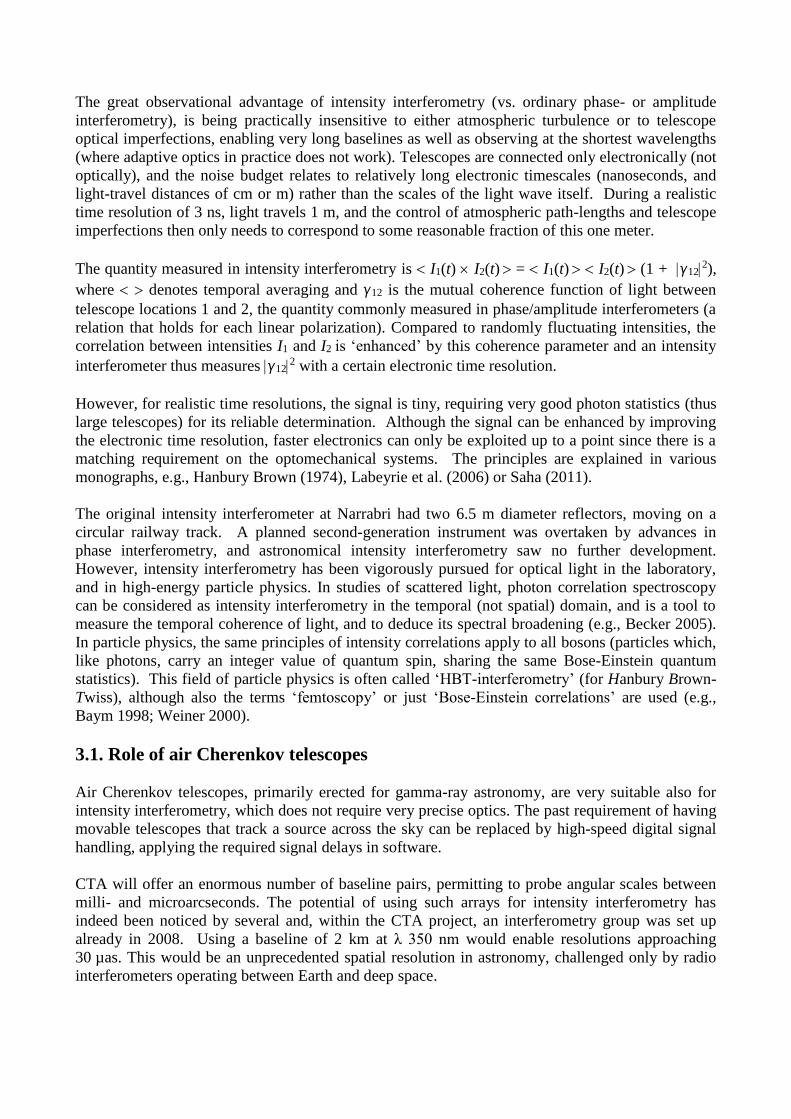
The great observational advantage of intensity interferometry (vs. ordinary phase- or amplitude

interferometry), is being practically insensitive to either atmospheric turbulence or to telescope

optical imperfections, enabling very long baselines as well as observing at the shortest wavelengths

(where adaptive optics in practice does not work). Telescopes are connected only electronically (not

optically), and the noise budget relates to relatively long electronic timescales (nanoseconds, and

light-travel distances of cm or m) rather than the scales of the light wave itself. During a realistic

time resolution of 3 ns, light travels 1 m, and the control of atmospheric path-lengths and telescope

imperfections then only needs to correspond to some reasonable fraction of this one meter.

The quantity measured in intensity interferometry is I1(t) I2(t) = I1(t) I2(t) (1 + 122),

where denotes temporal averaging and 12 is the mutual coherence function of light between

telescope locations 1 and 2, the quantity commonly measured in phase/amplitude interferometers (a

relation that holds for each linear polarization). Compared to randomly fluctuating intensities, the

correlation between intensities I1 and I2 is ‘enhanced’ by this coherence parameter and an intensity

interferometer thus measures 122 with a certain electronic time resolution.

However, for realistic time resolutions, the signal is tiny, requiring very good photon statistics (thus

large telescopes) for its reliable determination. Although the signal can be enhanced by improving

the electronic time resolution, faster electronics can only be exploited up to a point since there is a

matching requirement on the optomechanical systems. The principles are explained in various

monographs, e.g., Hanbury Brown (1974), Labeyrie et al. (2006) or Saha (2011).

The original intensity interferometer at Narrabri had two 6.5 m diameter reflectors, moving on a

circular railway track. A planned second-generation instrument was overtaken by advances in

phase interferometry, and astronomical intensity interferometry saw no further development.

However, intensity interferometry has been vigorously pursued for optical light in the laboratory,

and in high-energy particle physics. In studies of scattered light, photon correlation spectroscopy

can be considered as intensity interferometry in the temporal (not spatial) domain, and is a tool to

measure the temporal coherence of light, and to deduce its spectral broadening (e.g., Becker 2005).

In particle physics, the same principles of intensity correlations apply to all bosons (particles which,

like photons, carry an integer value of quantum spin, sharing the same Bose-Einstein quantum

statistics). This field of particle physics is often called ‘HBT-interferometry’ (for Hanbury Brown-

Twiss), although also the terms ‘femtoscopy’ or just ‘Bose-Einstein correlations’ are used (e.g.,

Baym 1998; Weiner 2000).

3.1. Role of air Cherenkov telescopes

Air Cherenkov telescopes, primarily erected for gamma-ray astronomy, are very suitable also for

intensity interferometry, which does not require very precise optics. The past requirement of having

movable telescopes that track a source across the sky can be replaced by high-speed digital signal

handling, applying the required signal delays in software.

CTA will offer an enormous number of baseline pairs, permitting to probe angular scales between

milli- and microarcseconds. The potential of using such arrays for intensity interferometry has

indeed been noticed by several and, within the CTA project, an interferometry group was set up

already in 2008. Using a baseline of 2 km at λ 350 nm would enable resolutions approaching

30 µas. This would be an unprecedented spatial resolution in astronomy, challenged only by radio

interferometers operating between Earth and deep space.

4. Optical image synthesis

The original intensity interferometer in Australia used two telescopes to ‘only’ deduce angular sizes

of stars. Multiple telescopes over numerous baselines enable more complete image reconstructions.

The van Cittert-Zernike theorem, fundamental for interferometric imaging, tells that the quantity

measured by a [phase] interferometer for a given baseline, is a component of the Fourier transform

of the surface intensity distribution of the source. Thus, multiple separations and orientations of

interferometric pairs of telescopes, sample the (u;v)-plane of the Fourier-transform, permitting to

reconstruct the source image with an angular resolution corresponding to the longest baseline.

In intensity interferometry, a certain complication enters since the correlation function for the

electric field in light is not directly measured, but only the square of its modulus. Since phase

information is not preserved, direct inversion of observations into images is not possible. However,

while not feasible with just one single pair of telescopes, this is enabled by large telescope arrays.

With many flux collectors, the number of baselines formed in software becomes very large: N

telescopes can form N (N1)/2 baseline pairs. With telescopes fixed on the ground, the baselines

trace out curves in the Fourier (u;v)-plane, as an object moves across the sky. With digital signal

handling, all measurements can be allocated to their specific (u;v)-coordinates, producing a highly

filled (u;v)-plane, with practically all orientations across the source image. Such complete data

coverage strongly constrains the image geometry, enabling reconstruction of the phases of the

Fourier components, and a full image reconstruction (except a non-uniqueness of mirror images).

For multiple telescopes, another advantage of intensity interferometry emerges. Since those are

connected by software only, there is no loss of signal when synthesizing any number of baselines:

the digital signal from each telescope is simply copied. By contrast, phase interferometry in the

optical (as opposed to radio) requires beams of actual starlight between the telescopes. For aperture

synthesis with many baselines, starlight from each telescope must then be split, diluted, and sent to

several others, each with its own optical delay-line system. While this might work for a small

number of telescopes, the complexity rapidly becomes unrealistic for any larger array.

5. Microarcsecond astrophysics

Tantalizing results from current optical interferometers (e.g., ESO VLTI, or CHARA in California)

– revealing circumstellar shells or oblate shapes of rapidly rotating stars – show how we are just

beginning to view stars as a vast diversity of objects, and a great step forward will be enabled by

improving angular resolution by merely another order of magnitude. Observing programs, listing

targets selected for both their astrophysical interest and practical observability have been prepared

(Dravins et al. 2012, 2013); the figure below highlights some types of envisioned early science:

Reconstructed image of a star with three hot spots from

simulated intensity interferometry observations with a CTA-

like array. The pristine image has a temperature of 6000 K,

and the spots have temperatures of 6500 K (top right and left)

and 6800 K (lower). ‘PSF’ shows the theoretical resolution

limit. These data correspond to a star of apparent brightness

mv = 3 and 10 hours of integration (Nuñez et al. 2012).

Targets for kilometer-scale optical interferometry. Top: Stellar shapes and surfaces affected by rapid rotation –

The shape of Achernar; expected equatorial bulge and polar brightening of a very rapid rotator; deduced surface

brightness of the rapid rotator Vega, seen pole-on; possible donut-shape for a rapidly and differentially rotating star.

Middle: Disks and winds – Circumstellar disk of the Be-star ζ Tau; stellar winds compress circumstellar disks;

magnetic fields distort stellar-wind outflows; wind in a binary opens up cavities around the other star (the Wolf-

Rayet star 2 Vel deduced from interferometry). Bottom: Stellar surroundings – Interferometric image of T Lep

surrounded by its molecular shell; the giant Aur, partially obscured by a circumstellar disk; artist’s view of the

interacting Lyr system; adaptive-optics image of Car, the brightest star in the Galaxy. (Dravins et al. 2013)

A vision of future microarcsecond optical imaging: Expected resolution for an assumed transit of a hypothetical

exoplanet across the disk of Sirius, using the Cherenkov Telescope Array as an intensity interferometer. Stellar

diameter = 1.7 solar, Distance = 2.6 pc, Angular diameter = 6 mas; assumed planet of Jupiter size and oblateness;

Saturn-type rings; four Earth-size moons; equatorial diameter = 350 µas. With the CTA array spanning 2 km, a 50

µas resolution provides more than 100 pixels across the stellar diameter. (Dravins & Lagadec 2014)

6. Potential of the ASTRI Mini-array

The layout of the ASTRI mini-array foresees 5, 7 or perhaps even 9 telescopes with telescope-pair

separations of ~300 m. Even if only a small subset of the full CTA, such a layout makes the array

attractive for intensity interferometry. With maximum baselines extending to ~700 meters, the

angular resolution obtainable at 400 nm, say, would require a baseline of more than 3 km at 1.8

µm, that near-infrared wavelength that often is used in interferometers. The mini-array could thus

improve the resolution by an order of magnitude beyond what currently is reached with the largest

ground-based phase/amplitude optical interferometers. All other existing groups of Cherenkov

telescopes are more tightly positioned and cannot cover the corresponding parameter space.

7. Potential of the ASTRI prototype telescope

With only one telescope, possible observations are somewhat limited in scope but – even if not

reaching into new astrophysical domains – a number of measurements should still be possible.

The intensity-fluctuation signal measured in one single telescope can be written as I1(t) I1(t)

which equals I1(t) I1(t) (1 + 112) , and thus is a function of the spatial coherence function

112 of the source, averaged over the collecting area of that single telescope. In case the source is

of small angular extent, i.e., spatially not resolvable by a baseline equal to the telescope diameter,

there is full coherence over the telescope area and 112 = 1. However if the source is incoherent,

for example of large angular size or a binary star, 112 is correspondingly less, as is the intensity-

fluctuation signal. Comparisons between measurements of single small stars and of large or binary

ones would illustrate realistic signals for intensity interferometry and permit to identify possible

noise sources and methods for optimizing observations without awaiting the full mini-array.

In principle, this intensity-fluctuation signal could be obtained as the temporal autocorrelation of the

measured stellar flux. In practice, however, auto-correlations are not likely to provide adequately

useful data, the reason being various detector imperfections, in particular afterpulsing. Every type

Planned layout on the ground for the ASTRI mini-array envisions maximum baselines up to some 700 meters,

significantly longer than any other current array of Cherenkov telescopes. (Gabriele Rodeghiero: Intensity

Interferometry with the ASTRI/CTA mini array, Workshop on Hanbury-Brown and Twiss Interferometry,

Observatoire de la Côte d’Azur, Nice, 2014)

of detector is likely to show some degree of correlated false signals. Even if the afterpulsing

probability is ‘tiny’, a fraction of one percent, it immediately appears in the correlation functions,

mimicking true astrophysical correlations. Examples of afterpulsing signatures for silicon

avalanche diodes (SPADs) are shown in Section 8.4 below. Those for photomultipliers are

qualitatively similar, except that certain discrete timescales can be identified and traced to electron

travel times between different dynodes.

This problem practically disappears if one instead computes the cross-correlation of the signal

between two different detectors. Afterpulsing and other parasitic signals are not correlated in time

between separate detectors, and (except for very small higher-order effects) the cross-correlation

signal is ‘clean’ from detector imperfections.

This is the procedure foreseen for intensity interferometry, measuring the signals between different

and separated telescopes. For measuring the one signal in a single telescope, one could introduce a

beamsplitter that divides the light and directs half of it to each of two different detectors, whose

outputs are then cross-correlated. (A procedure used in our laboratory measurements.)

However, it turns out that such arrangements are not needed. The point-spread-function of the

ASTRI telescope is such, that on its present SiPM detector, it covers two of its neighboring detector

‘pixels’ of 33 mm2 each, whose signals are independently processed. Each cell of these in

principle records the same astrophysical signal, and an intensity cross-correlation between both

detector cells in principle yields the telescope-aperture averaged spatial coherence of the source.

However, it must be cautioned that multi-element semiconductor detectors might well possess some

nontrivial properties (optical or electronic crosstalk, optical afterglow, or other) that might appear at

some level also in the cross-correlation functions. Even if such signatures exist, they need not be

problematic if they are stable over time and can be calibrated. Already a short observing run should

be sufficient to indicate possible such issues.

It can also be noted that the correlator electronics will provide also the autocorrelation functions for

all detectors, and thus tell about their possible afterpulsing, and other statistical properties.

8. Observing with the ASTRI prototype telescope

8.1. Constraining stellar fluxes with a color filter

To reach maximum signal-to-noise, it is desirable to observe bright targets. However, the flux from

bright stars can be overwhelming and must be moderated.

A very bright zero-magnitude star (such as Vega) has a flux in the visual V-band on the order of one

million photons/s/cm2. An ASTRI-sized telescope (~10 m2) will then collect ~1011 photons/second.

Assuming a system throughput of atmospheric and telescopic transmissions, detector quantum

efficiency, etc., of 10%, say, then implies photon rates of ~10 GHz. However, such count rates

cannot be handled, and must be reduced by perhaps two orders of magnitude to ~100 MHz or less.

Signal-to-noise in intensity interferometry has the (perhaps non-intuitive) property of in principle

being independent of the optical bandpass, be it wide-band white light or a narrow spectral line.

The smaller photon flux in the latter case is exactly compensated by the correspondingly longer

optical coherence time. The same applies to linearly polarized light: in each polarization, the light

flux is reduced, causing more photon noise, but that is compensated by an enhanced physical signal.

(These properties imply that S/N in intensity interferometry could be improved by simultaneous

measurements in multiple spectral bandpasses, although that is not a current option with ASTRI.)

Thus, in order to maintain the S/N while decreasing the photon flux to practical levels, it is required

to use some color filter with a narrow optical bandpass, on order of 1% of the optical range, i.e.,

~5 nm. Such are commonly available as interference filters on plane substrates. However, their

functioning presupposes that light is collimated to be parallel and incident perpendicular to the filter

surface. Light incident under other angles will have the transmitted wavelength shifted, and light

with a variety of angles will have the effective filter transmission widened.

The Schwarzschild–Couder optical system of the ASTRI telescope is extremely fast, f/0.5. In front

of the detector, a small filter should be placed. It seems not practical to introduce additional optics

to collimate the light but the use of a conventional interference filter in that location will cause a

poorly defined transmission due to the strongly differing angles of incoming light of the fast beam.

A possible solution could be an interference filter on a strongly curved surface, where the incoming

light would be perpendicular to it, and thus obtain a well-defined wavelength transmission. An

equivalent solution might be a plane filter, but where the thickness of the interference layers

gradually change in a radially symmetric manner from its center, to compensate for the gradually

changing angles of incident light. It is not clear, whether such filters can be produced and if so, at

what cost, but inquiries have been sent to a few optical companies (Altechna, Andover, Knight).

Further options could include mounting several small plane interference filters onto a roughly

spherical structure (maybe in pentagonal and hexagonal segments forming part of a classical

football?), in order to at least approximately match the angles of the incoming light.

Narrow-band filters can also be based on other optical principles, such as “Christiansen filters”.

These consist of an optical cell with crushed glass immersed in a liquid. At that wavelength where

the indices of refraction for glass and liquid are equal, the cell is transparent, while at all other

wavelengths, the light is reflected, scattered or refracted away at the many interfaces between the

tiny glass pieces and the liquid. Bandpasses on order ~10 nm have been documented in the

literature, but we are not aware of any commercial suppliers.

If schemes such as these would not be practical, ordinary broader-band glass filters made with color

dyes could be used, with another sharp-cut filter in series. This would constitute the simplest short-

term solution although they would probably not provide a very narrow wavelength selection nor the

highest transmission, but should anyway be adequate for any initial observations.

8.2. Digital correlators

An essential element of an intensity interferometer is the correlator, which provides the temporally

averaged product of the intensity fluctuations I1 I2 in two telescopes, normalized by the

product of average intensities in each of them, I1 I2.

Photon correlators are commercially available for primary applications in light scattering against

laboratory specimens. Based upon experiences from previous hardware correlators from different

manufacturers, current units available at Lund Observatory were custom-made (by Correlator.com)

for applications in intensity interferometry, featuring sampling frequencies up to 700 MHz, able to

handle continuous photon-count rates of more than 100 MHz per channel without any deadtimes,

and with on-line data transfer to a host computer. Their output contains the cross correlation

function between pairs of telescopes (as well as autocorrelation functions for each of them), made

up of about a thousand points. For small delays, the sampling is made with the shortest timesteps of

just a few ns, increasing in a geometric progression to large values to reveal the full function up to

long delays of even seconds or more. Nominal price per correlator unit is on order ~10 k€.

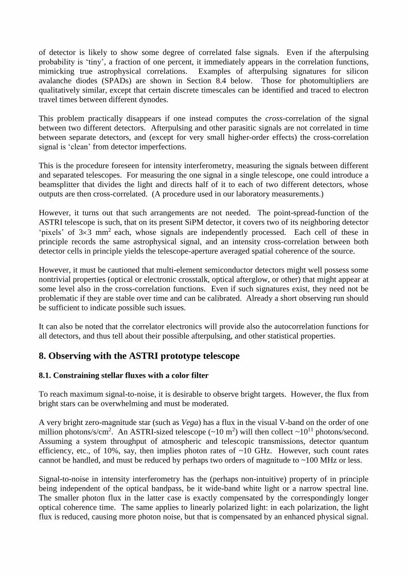
Digital photon correlators used in laboratory experiments, and planned for ASTRI. These particular ones are based

upon Field Programmable Gate Arrays (FPGA) with 700 MHz clock rate, 1.4 ns time resolution, handling up to 200

MHz photon-count rates at TTL-level voltages. Each of these handles signals from eight telescopes simultaneously.

The size of each box is slightly below 12104 cm, with the USB and BNC connectors protruding some additional

cm. Our other correlators have somewhat differing electronic parameters but the same physical size.

The inside of a digital 8-channel hardware correlator.

Electronic principles of digital photon correlators: Correlation functions are produced in real time, processing large

amounts of data, eliminating the need for their further handling and storage (e.g., one channel running at 50 MHz

during an 8-hour observing night processes more than 1 TB. A disadvantage is that, if something needs to be

checked afterwards, the original data are no longer available, and alternative signal processing cannot be applied.

Correlator operation: The detectors measure the intensity of the light I(t) and their output signals are fed to the

correlator via coaxial cables. It calculates the temporal correlation between the two signals, i.e., I1(t) I2(t +t).

The correlator also normalizes the function, so that it goes towards the value 1 for long delay times. The correlation

functions are sent to a computer through a USB 2.0 port. (Tiphaine Lagadec, MSc thesis, Lund Observatory, 2014)

Even if the correlators usually perform as expected, these are research-class devices and do not have

consumer-class reliability nor documentation. Their software runs under Windows 32-bit operating

systems (the hardware drivers are specific to the 32-bit versions) and, from experience, one should

avoid running other applications simultaneously on the host computer. They actually offer several

further computing modes, which have as yet not been much explored, including the possibility to

store the entire photon-pulse stream to computer (for moderate count rates). What is then stored is

not some absolute time-tag but rather a sequence of numbers that specify the number of correlator

clock cycles (in units of a few ns) that have elapsed since the previously recorded photon count.

It should also be noted that, for realistic observations in intensity interferometry, the desired signal

is only a small fraction of the full (Poisson-noise) intensity correlation in the raw data, and the

signal must be analyzed to many decimal digits, differentially to calibration measurements.

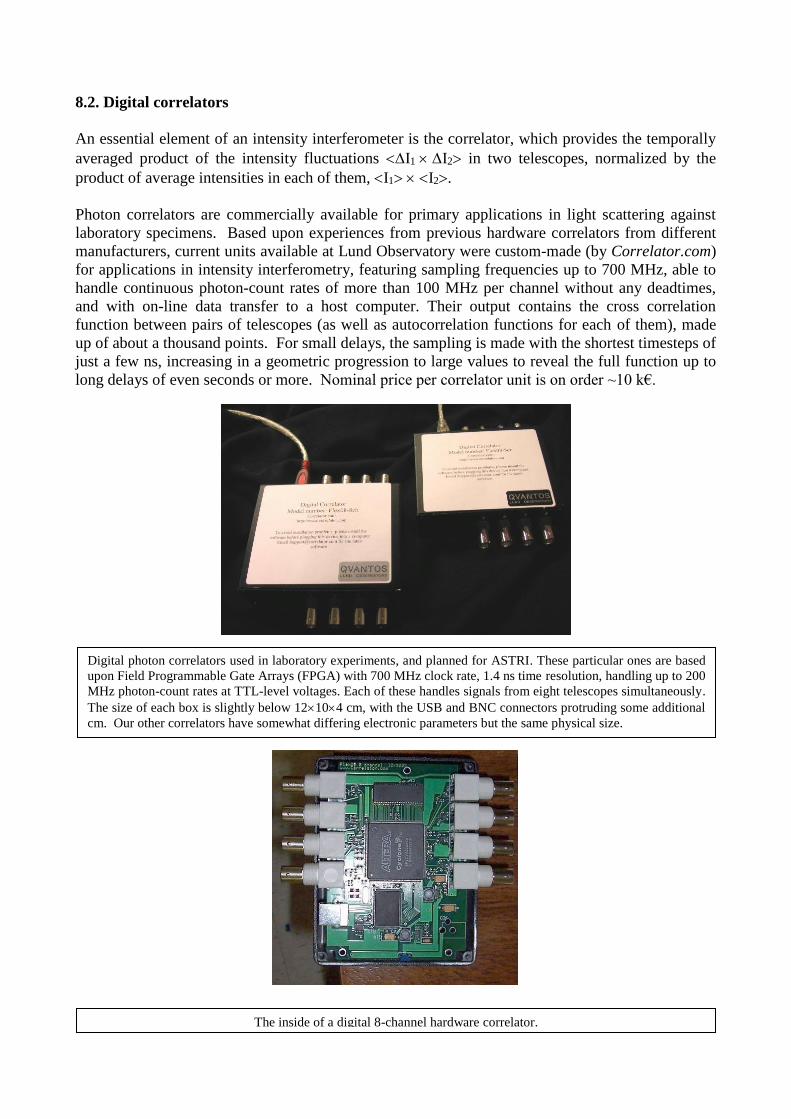
Sample computer screenshot of the correlator software interface. Among the correlation modes offered, here the

‘QUAD-mode’ is used for the signals entering channels A and B, to simultaneously obtain all auto- and cross-

correlations (AA, BB, AB and BA). Integration time is selected at the bottom. To start measurements, one

clicks ‘START’. The intensity trace at top right shows the (possibly varying) intensity during the integration; the

instantaneous count rates for both channels are in bottom left. The two main windows show the four correlations.

After the integration, a click on the ‘save’ button stores the file in a specific *.SIN format. (Tiphaine Lagadec, MSc

thesis, Lund Observatory, 2014)

8.3. Understanding correlation functions

The correlation functions reveal the timescales of source variability. These sample measurements

illustrate how optical variability is detected on timescales differing by many orders of magnitude:

8.4. Characterizing detector properties

When analyzed with sufficient precision, all detectors display some kind of imperfections or

specific signatures. The examples below serve as examples of such, which can be studied with

correlators. These are for single-photon-counting silicon avalanche photo-diodes (SPADs). They

are operated in ‘Geiger mode’, where each detected photon triggers an electronic avalanche as a

signature of photon detection. Following a detection, a certain deadtime occurs, during which

further detections are not possible. In addition to dark counts, detectors also show some level of

afterpulsing. There remains a possibility that an avalanche electron occasionally is caught in the

potential well around some semiconductor impurity site. If that trapped electron is released after a

time longer than the deadtime, it may trigger a new avalanche, correlated with the real photon

event. Since, in intensity interferometry, one searches for correlated signals, such afterpulsing may

appear as a false correlation. Of course, the afterpulsing is a property inside each one detector and

will not (except as a small higher-order effect) be correlated between two separate ones.

Correlation functions of fluctuations in intensity reveal variability on timescales over many orders of magnitude.

Here, laboratory measurements of three different classes of sources are shown: (a) A stabilized He-Ne laser is

constant over all timescales. (b) A xenon arc lamp is stable on short timescales but periodically variable on scales

of a fraction of a second. (The mechanism is modulation of the emission arc by the acoustic noise from the rotating

cooling fan.) (c) A blue 442 nm He-Cd laser is stable on longer timescales but variable over very short

timescales, with frequencies around 200 kHz. (The mechanism is plasma oscillations, a phenomenon known for

these particular lasers). (D.Dravins, H.O.Hagerbo, L.Lindegren, E.Mezey & B.Nilsson; Lund Observatory)

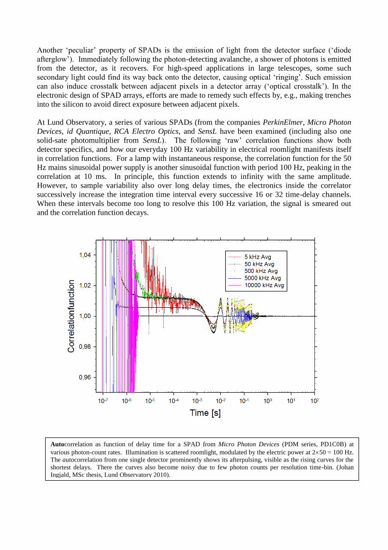
Another ‘peculiar’ property of SPADs is the emission of light from the detector surface (‘diode

afterglow’). Immediately following the photon-detecting avalanche, a shower of photons is emitted

from the detector, as it recovers. For high-speed applications in large telescopes, some such

secondary light could find its way back onto the detector, causing optical ‘ringing’. Such emission

can also induce crosstalk between adjacent pixels in a detector array (‘optical crosstalk’). In the

electronic design of SPAD arrays, efforts are made to remedy such effects by, e.g., making trenches

into the silicon to avoid direct exposure between adjacent pixels.

At Lund Observatory, a series of various SPADs (from the companies PerkinElmer, Micro Photon

Devices, id Quantique, RCA Electro Optics, and SensL have been examined (including also one

solid-sate photomultiplier from SensL). The following ‘raw’ correlation functions show both

detector specifics, and how our everyday 100 Hz variability in electrical roomlight manifests itself

in correlation functions. For a lamp with instantaneous response, the correlation function for the 50

Hz mains sinusoidal power supply is another sinusoidal function with period 100 Hz, peaking in the

correlation at 10 ms. In principle, this function extends to infinity with the same amplitude.

However, to sample variability also over long delay times, the electronics inside the correlator

successively increase the integration time interval every successive 16 or 32 time-delay channels.

When these intervals become too long to resolve this 100 Hz variation, the signal is smeared out

and the correlation function decays.

Autocorrelation as function of delay time for a SPAD from Micro Photon Devices (PDM series, PD1C0B) at

various photon-count rates. Illumination is scattered roomlight, modulated by the electric power at 250 = 100 Hz.

The autocorrelation from one single detector prominently shows its afterpulsing, visible as the rising curves for the

shortest delays. There the curves also become noisy due to few photon counts per resolution time-bin. (Johan

Ingjald, MSc thesis, Lund Observatory 2010).

8.5. Electronic connection to the correlator

‘Clean’ plot showing detector deadtime and afterpulsing. The autocorrelation of measured intensity in this

particular SPAD detector is zero below 80 ns which is its deadtime, within which only one photon can be recorded

(the effect also seen as a small bump at twice that value). For the shortest delay times, the autocorrelation rises due

to afterpulsing. Although its probability after any photon detection is small, it stands out strongly in the statistics.

For delays beyond 1 µs, the autocorrelation seen in this particular measurement is physical. In cross-correlation

between the signals from two separate detectors (without physical correlation), these instrumental effects practically

vanish since afterpulsing is rare and not correlated between different detectors. (Dravins & Lagadec 2014)

Cross-correlation as function of delay time between two SPADs from Micro Photon Devices (PDM series,

PD1C0B) at various photon-count rates. Illumination is scattered roomlight, modulated by the electric mains power

at 250 = 100 Hz. The cross-correlation between two detectors essentially eliminates signatures from afterpulsing

at short delay times. (Johan Ingjald, MSc thesis, Lund Observatory 2010).

8.5. Electronic connection to the correlator

The figure below shows typical photon-detection pulses produced by SPAD modules used for

intensity interferometry experiments in the laboratory. It is a stream of such pulses (of TTL

standard) that, through 50 BNC coaxial cables, are fed to the correlator for real-time computation

of various statistical functions. Laboratory experiments have shown no noticeable degradation for

cable lengths of up to 20 meters (longer ones have not been tried).

The width of these pulses reflect the deadtimes and the pulse-shaping electronics of the SPAD

modules. For some of our correlators, experiments have been performed to check what are the

minimum pulse widths and amplitudes, where the correlators still perform normally. It seems that

the pulse amplitude can be decreased significantly from the normal 5 V value to about 2 V without

noticeable effects, but not much below such a value. The pulse-width can also be decreased

significantly, probably to 10 ns or less (although all combinations of amplitudes and widths have

not been tested). Maximum sustained count rates into the correlators have been around 40 MHz per

input channel. Such values are higher than the deadtime-limited maximum rates from SPAD

modules but were achieved by high-speed digitization of photomultiplier signals.

It appears that a suitable mode of operation at ASTRI would involve the digitization of the detector

outputs, then shaping pulses for each photon detection, adjusting the amplitudes and pulse-widths to

reach the maximum count rates that can be safely processed by the correlator.

8.6. Observing targets for intensity interferometry

The ‘easiest’ targets for tests of intensity interferometry are bright and hot single stars of small

angular size, producing a spatially coherent signal across the full telescope aperture. For measuring

an incoherent signal (where the stellar diameter is resolved across the telescope aperture), any

bright red-giant star can be used, or – for more precise measurements – some binary star with

known component separation and brightness.

Examples of stars unresolved by a single ASTRI telescope (single stars without bright components),

observable during different seasons of year:

Examples of pulse shapes from a SPAD detector module, measured by a digital oscilloscope for different photon-

count rates (from left: 50 kHz, 500 kHz, 5000 kHz). These form the stream of TTL pulses that are sent from the

detector over a coaxial BNC cable to the correlator. (Johan Ingjald, MSc thesis, Lund Observatory 2010).

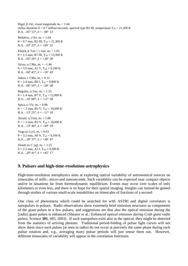
Rigel, Ori, visual magnitude mv = 1.64

stellar diameter = 0.7 milliarcseconds, spectral type B2 III, temperature Teff = 21,300 K

R.A. = 05h 15m, = 08 12

Bellatrix, Ori, mv = 1.64

= 0.7 mas, B2 III, Teff = 21,300 K

R.A. = 05h 25m, = +06 21

Elnath, Tau = Aur, mv = 1.65

= 1.5 mas, B7 III, Teff = 13,500 K

R.A. = 05h 26m, = +28 36

Sirius, CMa, mv = 1.46

= 5.9 mas, A1 V, Teff = 9,100 K

R.A. = 06h 45m, = 16 43

Adara, CMa, mv = 0.12

= 2.4 mas, B8 I, Teff = 9,800 K

R.A. = 06h 59m, = 28 58

Regulus, Leo, mv = 1.35

= 1.4 mas, B7 V, Teff = 12,000 K

R.A. = 10h 08m, = +11 58

Spica, Vir, mv = 0.98

= < 2 mas, B3 V, Teff = 18,000 K

R.A. = 13h 25m, = 11 10

Alcaid, Uma, mv = 1.86

= < 2 mas, B3 V, Teff = 18,000 K

R.A. = 13h 48m, = +49 19

Vega ( Lyr), mv = 0.03

= 3.2 mas, A0 V, Teff = 9,100 K

R.A. = 18h 37m, = +38 47

Deneb ( C yg), mv = 1.25

= 2.2 mas, A2 I, Teff = 9,300 K

R.A. = 20h 41m, = +45 17

9. Pulsars and high-time-resolution-astrophysics

High-time-resolution astrophysics aims at exploring optical variability of astronomical sources on

timescales of milli-, micro-and nanoseconds. Such variability can be expected near compact objects

and/or in situations far from thermodynamic equilibrium. Events may occur over scales of only

kilometers or even less, and there is no hope for their spatial imaging. Insights can instead be gained

through studies of various small-scale instabilities on timescales of fractions of a second:

One class of phenomena which could be searched for with ASTRI and digital correlators is

nanopulses in pulsars. Radio observations show extremely brief emission structures as components

of the giant pulses in a few pulsars, and suggestions are that also the optical emission during the

[radio] giant pulses is enhanced (Shearer et al.: Enhanced optical emission during Crab giant radio

pulses, Science 301, 493, 2003). If such nanopulses exist also in the optical, they might be detected

from the statistics of arriving photons. Traditional period-folding of pulsar light curves will not

show them since such pulses (at seen in radio) do not occur at precisely the same phase during each

pulsar rotation and, e.g., averaging many pulsar periods will just smear them out. However,

different timescales of variability will appear in the correlation functions:

The point-spread function in Cherenkov telescopes gives a significant contribution from the night-

sky background. However, on very short timescales of microseconds and less, this background

actually is very modest. In the optical, the Crab pulsar has been observed with different Cherenkov

telescopes:

Analogous light-curves for the Crab pulsar have been measured with H.E.S.S. (Franzen et al.:

Optical observations of the Crab pulsar using the first H.E.S.S. Cherenkov Telescope, The 28th

International Cosmic Ray Conference, 2003) and with HEGRA (Oña-Wilhelmi et al., Determination

of the night sky background around the Crab pulsar using its optical pulsation, Astropart.Phys. 22,

95, 2004).

Autocorrelation of the photon stream from the Crab pulsar, measured with the 1.3 m telescope at the Skinakas

Observatory on Crete, using silicon SPAD detectors in the OPTIMA instrument from MPE, Max-Planck-Institute

for Extraterrestrial Physics in Garching, real-time processed by digital correlators from Lund Observatory. The first

two maxima of the autocorrelation function around 10 ms indicate the times between the main pulse and interpulse,

and vice versa; the first sharp peak marks the pulsar period of 33 ms; other peaks are harmonics. The rise below

1 µs is due to detector afterpulsing.

Optical flux from the Crab pulsar measured with the MAGIC central-pixel PMT in an analog mode. Observations

over 20 minutes were period-folded. (Lucarelli et al.: Development and first results of the MAGIC central pixel

system for optical observations, The 29th International Cosmic Ray Conference, 2005)

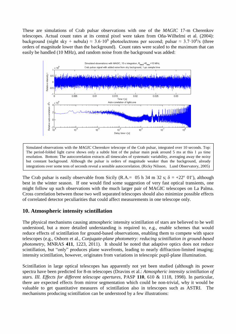
These are simulations of Crab pulsar observations with one of the MAGIC 17-m Cherenkov

telescopes. Actual count rates at its central pixel were taken from Oña-Wilhelmi et al. (2004):

background (night sky + nebula) ≈ 3.6·109 photoelectrons per second; pulsar ≈ 3.7·106/s (three

orders of magnitude lower than the background). Count rates were scaled to the maximum that can

easily be handled (10 MHz), and random noise from the background was added:

The Crab pulsar is easily observable from Sicily (R.A.= 05 h 34 m 32 s; = +22 01), although

best in the winter season. If one would find some suggestion of very fast optical transients, one

might follow up such observations with the much larger pair of MAGIC telescopes on La Palma.

Cross correlation between those two well separated telescopes should also minimize possible effects

of correlated detector peculiarities that could affect measurements in one telescope only.

10. Atmospheric intensity scintillation

The physical mechanisms causing atmospheric intensity scintillation of stars are believed to be well

understood, but a more detailed understanding is required to, e.g., enable schemes that would

reduce effects of scintillation for ground-based observations, enabling them to compete with space

telescopes (e.g., Osborn et al., Conjugate-plane photometry: reducing scintillation in ground-based

photometry, MNRAS 411, 1223, 2011). It should be noted that adaptive optics does not reduce

scintillation, but “only” produces plane wavefronts, leading to nearly diffraction-limited imaging;

intensity scintillation, however, originates from variations in telescopic pupil-plane illumination.

Scintillation in large optical telescopes has apparently not yet been studied (although its power

spectra have been predicted for 8-m telescopes (Dravins et al.: Atmospheric intensity scintillation of

stars. III. Effects for different telescope apertures, PASP 110, 610 & 1118, 1998). In particular,

there are expected effects from mirror segmentation which could be non-trivial, why it would be

valuable to get quantitative measures of scintillation also in telescopes such as ASTRI. The

mechanisms producing scintillation can be understood by a few illustrations:

Simulated observations with the MAGIC Cherenkov telescope of the Crab pulsar, integrated over 10 seconds. Top:

The period-folded light curve shows only a subtle hint of the pulsar main peak around 5 ms at this 1 μs time

resolution. Bottom: The autocorrelation extracts all timescales of systematic variability, averaging away the noisy

but constant background. Although the pulsar is orders of magnitude weaker than the background, already

integrations over some tens of seconds reveal a sensible autocorrelation. (Ricky Nilsson, Lund Observatory, 2005)

Pupil image (telescope main mirror, with secondary-mirror obscuration visible) for a bright star. Brighter and

darker patches are ‘flying shadows’ from starlight caused by upper-atmospheric turbulence. Intensity scintillation

results from incomplete intensity averaging of this pattern as it is both intrinsically evolving, and carried by winds.

(1 ms exposure on a 1-m telescope on La Palma (Applied Optics group, Imperial College, London)

Atmospheric intensity scintillation: Shadow bands (‘flying shadows’) are seen on the ground during short moments

near solar-eclipse totality, when the remaining fraction of the solar disk takes on the character of a point source

This painting shows shadow bands moving across a house in Sicily(!) during a solar eclipse in 1870. A stationary

observer perceives these patterns as rapid fluctuations of intensity. (Codona, Sky & Tel. 81, 482, 1991)

Sunlight patterns on the bottom of a pool of water are determined by refraction in random ‘lenses’ formed at the

water surface. If the water is flowing like a river, the effects are analogous to ‘flying shadows’ in air.

On first sight, it would appear that large telescopes should perceive only very small amounts of

scintillation, given their large averaging apertures. However, the scintillation signal might be quite

complex because the entrance pupil (in e.g., E-ELT and ASTRI) is incompletely filled in a because

of the narrow gaps between the primary-mirror segments. This makes them sensitive to small

spatial scales of scintillation and the gap orientation makes them sensitive to also the direction of

flying shadows, i.e., to the direction of the atmospheric wind velocity.

If the wind and its ensuing flying shadows are parallel to the mirror gaps, there will be some

averaging along the full length of these gaps, but if it is perpendicular to those, there will be a

filtering on the small scale of the distance between adjacent mirror segments. Of course, whether

this will influence some particular observations may be determined by how precisely, i.e. to which

decimal place one can push any measurements.

Since scintillation originates from the projected intensity pattern on the telescope entrance pupil,

thus occurs before any telescopic focusing of the light, and is insensitive to atmospheric or

instrumental phase errors (which affect the diffraction and the focused image), and therefore can be

fully measured also by Cherenkov telescopes such as ASTRI, despite their limited imaging quality.

In this case, what is needed is a star that is sufficiently much brighter than the sky background in

order for that not to contribute significantly. The flux on the detector can be adjusted to the desired

level by some neutral or broad-band color filter; interference filters are not required.

The scintillation signal in large apertures is bound to be quite small and require correspondingly

sensitive methods for detection; high-speed photon-counting and subsequent signal analysis with

correlation electronics should be suitable here. Calibration against some (almost) non-scintillating

source will require one of large angular extent, perhaps part of the Moon or a planet.

Simulated ‘flying-shadow’ pattern on an extremely large telescope. Besides scintillation in intensity, diffraction by

this pattern throws parasitic light into the far wings of any focused stellar image. Suppression of this effect is

essential to enable direct imaging of faint extrasolar planets close to their host stars. (Hubin et al.: EPICS, Earth-

like planets imaging camera spectrograph, ESO OWL instrument concept study, 2005)

11. Characterizing mechanical vibrations

Correlation functions can reveal ‘all’ variability in measured starlight, both intrinsic and such

caused by the instrumentation. The latter include vibrations of the telescope itself, caused by wind

gusts or perhaps irregularities in tracking. The sensitivity to detecting such effects is greater for a

conventional telescope focusing a small stellar image onto a small detector, but might well be

applicable also to ASTRI, and used to supplement the characterization of its telescope mechanics.

12. Preparations for observing

12.1. Preparing the detector and its ancillary filter mount

It is understood that a photon-counting detector unit will be placed at a central location in the focal

plane. In order to analyze the output with the presently available correlators, the outputs from the

two adjacent ‘pixels’ of 33 mm2 in the detector have to be formatted into TTL-type pulse streams,

connecting to the correlator via BNC cables (as described in Sect. 8.5 above).

An important component is some mechanical arrangement that enables the mounting of optical

filters in front of the detector. For intensity interferometry, good S/N ratios requires observing

bright stars with the highest possible photon-count rates that can be handled. However, bright stars

could generate extremely high count rates which must be reduced by optical filters. Detector

properties could be measured with any simple neutral filter, but to retain the physical signal

measurable by intensity interferometry requires the reduction in photon flux to be made by a filter

with a narrow bandpass in wavelength. Due to the telescope’s extremely fast optical system, this is

somewhat challenging since an ordinary plane interference filter will not retain its wavelength

transmission profile due to the variable angles of incident light (as described in Sect. 8.1 above).

For experiments in observing faint sources (such as the Crab Pulsar) or for studying atmospheric

scintillation, these restrictions do not apply. It is understood that expected count rates from each

pixel during a moonless night may be around 12 MHz, reaching upwards of 100 MHz during a full-

Moon night. Since the dark signal is only small fraction of these values, the count rates can be

Identifying telescope vibrations in real time: Vibrations of the 1.3 m telescope of the Skinakas Observatory on

Crete are excited when pointing the telescope into the direction of a strong wind. Oscillation features at timescales

~ 0.15 s, corresponding to ~ 6.8 Hz, are prominent in the measured autocorrelation functions of two different stars

and identify the resonance frequency of the mechanical telescope structure. (Ricky Nilsson, MSc thesis, Lund

Observatory, 2005)

adjusted to practical values by an ordinary color dye filter or a combination of two filters in series,

possibly combined with also a polarizer.

The first priority should then be some ‘simple’ mechanical mount to enable the placement of two

or three ordinary glass filters on top of another, close in front of the detector. Depending on

available space, suitable dimensions of each filter are either 25 mm circular or 50 mm square, 3 mm

thick, sizes readily available from commercial suppliers.

Such a filter mount will enable a series of measurements that should be able to characterize the

detector suitability for intensity interferometry, enable some pulsar observations, and provide some

measurements of atmospheric intensity scintillation. At this time of writing, the optimum optical

solution for incorporating also truly narrow-band filters is not clear, and it is suggested to consider

that as ‘second priority’, until more experience has been gained with mounting the ‘simpler’ filters.

12.2. Purchase of additional equipment

Some funds are available at Lund Observatory for laboratory and field experiments in intensity

interferometry, high-speed astrophysics, and the like. From existing grants, there is still (at this

time of writing) an amount of almost 15 k€ remaining, out of which perhaps up to one half could be

used for purchases needed in these experiments (these funds are thus available already now).

Another application to a local academy for a new grant is pending, with a decision expected in

November. In the use of these funds, however, some rules must be followed:

Important 1: These funds may be used for the purchase of any ‘items’ (i.e., equipment,

instrumentation, apparatus, components, software, etc.) but can not be used to pay any salaries,

honoraria, or other costs for personnel.

Important 2: The items purchased may be placed at any suitable location (Serra La Nave, Catania,

Lund, or elsewhere). However, irrespective of to where the items are delivered, for legal reasons, it

is only possible to pay invoices that are addressed by the seller to Lund University. It is thus not

possible to pay invoices addressed to some other institute or person. However, if another institute

would make a purchase, it is possible for that institute, in turn, to write another invoice addressed to

Lund University, specifying the expenses occurred. However, before making any purchases, please

contact us to specify the exact invoice address (different from our postal address), and the Lund

University VAT registration number (needed for purchases inside the EU).

Important 3: If a purchase reaches a significant sum (on order 1000 € or more), an effort should be

made to combine that purchase with others, to reach a total invoice sum of not less than 20,000 SEK

(approx. 2,100 €), exclusive of VAT. Our university regulations levy very significant overhead

costs (about 90%) onto ‘running costs’ but zero overhead if the transaction is larger and classified

as ‘investment’. The separation between these categories is defined as an invoice amount of SEK

20,000. Thus, a purchase of SEK 19,999 costs about twice as much for the grant, as a purchase of

SEK 20,001 ! I refrain from discussing the logic of this system but these are the current rules, at

least for 2014. It is not necessary that the ‘expensive’ item is one single piece: it can be a multitude

of things, but the items should somehow ‘belong together’ (which they will automatically do, if

they are all planned for ASTRI observations), and should be billed on the same invoice. If there has

been a first invoice that is above SEK 20,000, it can still be possible to avoid overhead also for

future smaller purchases made within 12 months of the first one, if it is explained that the items on

the smaller invoices belong together with the larger one. Again, before making any purchases,

please contact me to specify the detailed procedures.

12.3. Travels and observing runs

It is envisioned that ‘we’ (i.e., myself, probably together with some student or colleague) will visit

Sicily sometime around the timeframe late spring/early summer of 2015 to participate in a first

round of optical observations with the ASTRI telescope. We will then bring one or two correlators

(of which probably one can be left at Serra La Nave), together with software and a laptop computer

for its operation. For a first run of test observations, it seems reasonable to aim for something like 5

nights, in which case a total visit duration on the order of 10 days or so seems sensible, allowing

also a few days of evaluating quick-look data, and discussing prospects for possible further

observing runs. We will cover all our travel costs.

13. References

G.Baym: The physics of Hanbury Brown-Twiss Intensity Interferometry: From stars to nuclear collisions

Acta Physica Polonica B 29, 1839 (1998)

W.Becker: Advanced Time-Correlated Single Photon Counting Techniques. Springer (2005)

D.Dravins, T.Lagadec: Stellar intensity interferometry over kilometer baselines: Laboratory simulation of

observations with the Cherenkov Telescope Array, Proc. SPIE 9146, 91460Z (2014)

D.Dravins, S.LeBohec, H.Jensen, P.D.Nuñez: Stellar Intensity Interferometry: Prospects for sub-

milliarcsecond optical imaging, New Astron. Rev., 56, 143 (2012)

D.Dravins, S.LeBohec, H.Jensen, & P.D.Nuñez, for the CTA Consortium: Optical Intensity Interferometry

with the Cherenkov Telescope Array, Astropart. Phys., 43, 331 (2013)

D.Dravins, L.Lindegren, E.Mezey, & A.T.Young: Atmospheric Intensity Scintillation of Stars. III. Effects for

Different Telescope Apertures, Publ.Astron.Soc.Pacific, 110, 610-633, erratum: ibid. 110, 1118 (1998)

R.Hanbury Brown: The Intensity Interferometer. Taylor & Francis (1974)

A.Labeyrie, S.G.Lipson, P.Nisenson: An Introduction to Optical Stellar Interferometry. Cambridge (2006)

P.D.Nuñez, R.Holmes, D.Kieda, J.Rou, S.LeBohec: Imaging Sub-Milliarcsecond Stellar Features with

Intensity Interferometry Using Air Cherenkov Telescope Arrays, Mon.Not.Roy.Astron.Soc. 424, 1006 (2012)

S.K.Saha: Aperture Synthesis. Methods and Applications to Optical Astronomy. Springer (2011)

R.M.Weiner: Introduction to Bose-Einstein Correlations and Subatomic Interferometry. Wiley (2000)

-----------------------------------------------------------------------------------------------------------------------------------

-----------------------------------------------------------------------------------------------------------------------------------