intelligent decision support system for greenhosue tomato...
TRANSCRIPT

Decision Support Systems forGreenhouse Tomato Production
Item Type text; Electronic Dissertation
Authors Fitz-Rodriguez, Efren
Publisher The University of Arizona.
Rights Copyright © is held by the author. Digital access to this materialis made possible by the University Libraries, University of Arizona.Further transmission, reproduction or presentation (such aspublic display or performance) of protected items is prohibitedexcept with permission of the author.
Download date 28/04/2018 23:51:17
Link to Item http://hdl.handle.net/10150/195798
DECISION SUPPORT SYSTEMS FOR GREENHOUSE TOMATO PRODUCTION
by
Efrén Fitz-Rodríguez
________________________ Copyright © Efrén Fitz-Rodríguez 2008
A Dissertation Submitted to the Faculty of the
DEPARTMENT OF AGRICULTURAL AND BIOSYSTEMS ENGINEERING
In Partial Fulfillment of the Requirements For the Degree of
DOCTOR OF PHILOSOPHY
In the Graduate College
THE UNIVERSITY OF ARIZONA
2008
2
THE UNIVERSITY OF ARIZONA GRADUATE COLLEGE
As members of the Dissertation Committee, we certify that we have read the dissertation prepared by EFREN FITZ-RODRIGUEZ entitled DECISION SUPPORT SYSTEMS FOR GREENHOUSE TOMATO PRODUCTION . and recommend that it be accepted as fulfilling the dissertation requirement for the Degree of DOCTOR OF PHILOSOPHY ____________________________________________________Date: October 3, 2008 Dr. Gene A. Giacomelli ____________________________________________________Date: October 3, 2008 Dr. Chieri Kubota ____________________________________________________Date: October 3, 2008 Dr. Christopher Y. Choi ____________________________________________________Date: October 3, 2008 Dr. Young Jun Son Final approval and acceptance of this dissertation is contingent upon the candidate’s submission of the final copies of the dissertation to the Graduate College. I hereby certify that I have read this dissertation prepared under my direction and recommend that it be accepted as fulfilling the dissertation requirement. ___________________________________________________ Date: October 3, 2008 Dissertation Director: Dr. Gene A. Giacomelli

3
STATEMENT BY AUTHOR This dissertation has been submitted in partial fulfillment of requirements for an advanced degree at The University of Arizona and is deposited in the University Library to be made available to borrowers under rules of the Library. Brief quotations from this dissertation are allowable without special permission, provided that accurate acknowledgment of source is made. Requests for permission for extended quotation from or reproduction of this manuscript in whole or in part may be granted by the copyright holder.
SIGNED: Efrén Fitz-Rodríguez .

4
ACKNOWLEDGEMENTS I would like to thank my advisor and mentor Dr. Gene A. Giacomelli for his guidance, help and continuous support during the development of this research. An equal gratitude goes to Dr. Chieri Kubota for her support in reviewing each of the manuscripts and for being a role model not only as a scientist, but also as an educator. Many thanks to Dr. Christopher Y. Choi for his guidance in the beginning of my graduate studies and for giving me the opportunity of lecturing in his ABE 320 class, which gave me experience as an educator. My appreciation to Dr. Young Jun Son for the constructive criticism in the development of my dissertation. My infinite gratitude goes to Dr. Donald Slack for his continuous support during my graduate studies in the ABE department. A special appreciation to Dr. Merle Jensen for his vision in creating CEAC and for his continuous advice in practical and futuristic CEA applications. Many thanks to the rest of the CEAC faculty and staff that make the work at the CEAC interesting, and encourage me to work in this field of advanced agricultural technologies. My appreciation to the rest of the ABE faculty and staff that made it feel like home. Thanks to Kathleen Crist, Kimberly Heath, Daniela Ibarra and everyone else. To my friends and colleagues at the Controlled Environment Agriculture Center (Paula Costa, Nadia Sabeh, Jenn Nelkin, Armando Suarez, Min Wu, Ian Justus, Myles Lewis, Jason Licamele, José Chen and everyone else) who flavored the CEAC discussions with diverse and often with non CEA related topics.
CEAC Paper # T-125933-01-08. Supported by CEAC, the Controlled Environment Agricultural Center, College of Agriculture and Life Sciences, The University of Arizona. Financial support also provided by the United State Department of Agriculture, Cooperative State Research, Education, and Extension Service Higher Education Challenge Grant (3 years).

5
DEDICATION
To my lovely wife Ma. Cristina Ramirez-Ponce, who patiently waited for me on those
long nights of hard work and of studying, for her love, companionship, and endless
support, and for taking care of our “little corn tassel”, my infinite gratitude.
To my daughter Ahtziri –Little Corn Tassel, who spiced this journey of discovery in
science, for giving me the opportunity of relearning the human learning process, and for
all the joy she put into our lives.
To my parents Efrén and Fidelina who I love equally –I’m the product of your efforts.
To my siblings: Griselda, Gonzalo, Lluvia, Sol y Lucero – Never stop pursuing your
dreams.
6
TABLE OF CONTENTS
LIST OF FIGURES .......................................................................................................... 9
LIST OF TABLES .......................................................................................................... 10
ABSTRACT..................................................................................................................... 11
INTRODUCTION........................................................................................................... 13
BACKGROUND ......................................................................................................... 13 Definition of greenhouse crop production ............................................................ 13 Technological levels ................................................................................................ 14 Greenhouse crop production in North America .................................................. 15 Operational management of greenhouse production systems ............................ 16 The biophysical (crop-greenhouse) system ........................................................... 19
PROBLEM STATEMENT ........................................................................................ 24 LITERATURE REVIEW .......................................................................................... 29
Mechanistic and empirical models of the biophysical system............................. 29 Plant-based models ............................................................................................. 29 Greenhouse-oriented models.............................................................................. 31 Greenhouse-oriented models with optimization principles............................. 32
Decision-making in greenhouse production systems ........................................... 33 Intelligent decision support systems in greenhouse production systems ........... 37 Neural networks on greenhouse systems .............................................................. 38 Fuzzy logic on greenhouse systems........................................................................ 40
PROJECT OBJECTIVES.......................................................................................... 41 DISSERTATION FORMAT...................................................................................... 45
Proposed paper contribution 1: ............................................................................. 45 Proposed paper contribution 2: ............................................................................. 47 Proposed paper contribution 3: ............................................................................. 48
PRESENT STUDY.......................................................................................................... 49
OVERALL SUMMARY ............................................................................................ 49 DYNAMIC MODELING AND SIMULATION OF GREENHOUSE ENVIRONMENTS UNDER SEVERAL SCENARIOS: A WEB-BASED EDUCATIONAL APPLICATION (APPENDIX A) ........................................... 49 TOMATOES LIVE! 2.0: A WEB-BASED GREENHOUSE MONITORING SYSTEM (APENDIX B)......................................................................................... 50 YIELD PREDICTION AND GROWTH-MODE CHARACTERIZATION OF GREENHOUSE TOMATOES WITH NEURAL NETWORKS AND FUZZY LOGIC (APPENDIX C) ......................................................................................... 52
OVERALL CONCLUSIONS AND RECOMMENDATIONS ............................... 53
7
TABLE OF CONTENTS – Continued
REFERENCES................................................................................................................ 57
APPENDIX A: DYNAMIC MODELING AND SIMULATION OF GREENHOUSE ENVIRONMENTS UNDER SEVERAL SCENARIOS: A WEB-BASED EDUCATIONAL APPLICATION................................................................................ 67
ABSTRACT................................................................................................................. 68 INTRODUCTION....................................................................................................... 69 MATERIALS AND METHODS ............................................................................... 73
Climate data ............................................................................................................ 73 Greenhouse structure and components ................................................................ 74 Mathematical model ............................................................................................... 76 Energy balance equation ........................................................................................ 76 Mass (water vapor) balance equation ................................................................... 78 Numerical solution .................................................................................................. 79 Initial conditions ..................................................................................................... 80 Control functions .................................................................................................... 81
RESULTS AND DISCUSSION ................................................................................. 82 Greenhouse environment simulation with ventilation......................................... 83 Greenhouse environment simulation with evaporative cooling.......................... 84 Greenhouse environment simulation with shade curtains .................................. 85 Greenhouse environment simulation with heating .............................................. 86 Limitations of the model......................................................................................... 87
CONCLUSION ........................................................................................................... 88 REFERENCES............................................................................................................ 89
APPENDIX B: TOMATOES LIVE! 2.0: A WEB-BASED GREENHOUSE MONITORING SYSTEM............................................................................................ 104
ABSTRACT............................................................................................................... 105 INTRODUCTION..................................................................................................... 107
Description of greenhouse climate controllers ................................................... 108 Opportunities for improving the monitoring of greenhouse crops .................. 109 Internet technologies in greenhouse climate controllers ................................... 109 Motivation for further developments.................................................................. 110 Current status of greenhouse monitoring systems............................................. 111
NEW PROPOSED ARCHITECTURE................................................................... 113 Hardware and Infrastructure .............................................................................. 113
Data communication ......................................................................................... 114 Wireless infrastructure..................................................................................... 116 Visual monitoring.............................................................................................. 116
Software component ............................................................................................. 117

8
TABLE OF CONTENTS – Continued
Data collection and pre-processing.................................................................. 117 Plant-oriented climate summary ..................................................................... 119 Data storage and backup.................................................................................. 123 User interface .................................................................................................... 124
GENERAL DISCUSSION ....................................................................................... 125 FINAL REMARKS................................................................................................... 128 REFERENCES.......................................................................................................... 129
APPENDIX C: YIELD PREDICTION AND GROWTH-MODE CHARACTERIZATION OF GREENHOUSE TOMATOES WITH NEURAL NETWORKS AND FUZZY LOGIC .......................................................................... 131
ABSTRACT............................................................................................................... 132 INTRODUCTION..................................................................................................... 134 MATERIALS AND METHODS ............................................................................. 139
Crop records and climate data ............................................................................ 139 Neural network model .......................................................................................... 142
Input /output parameters ................................................................................. 143 Network architecture........................................................................................ 144 Network training ............................................................................................... 146
Fuzzy logic model .................................................................................................. 147 RESULTS AND DISCUSSION ............................................................................... 151
Neural network modeling..................................................................................... 151 Fuzzy modeling...................................................................................................... 154
CONCLUSION ......................................................................................................... 156 REFERENCES.......................................................................................................... 158

9
LIST OF FIGURES Figure 1. Relationships among the greenhouse production system phases and its
corresponding managerial level. ................................................................................ 17
Figure 2. Overall steps and processes within a greenhouses production system.............. 18
Figure 3. Diagram of the biophysical (crop-greenhouse) production system................... 19
Figure 4. Crop parameters used as inputs in the decision-making process of the operational management of the biophysical system. These parameters are the biological feedback to adjust the overall system. ...................................................... 20
Figure 5. Relationships of monitored plant conditions, directly or indirectly affected by each of the plant control mechanism managed by the greenhouse grower ............... 21
Figure 6. Weekly harvest rates variations among greenhouse managers in a commercial operation during two production cycles. ................................................................... 25
Figure 7. Total yield variation per week as a function of production area and several harvest rates differences. ........................................................................................... 27
Figure 8. Diagram of a feed-forward multi-layer perceptron showing its processing elements (nodes) and interconnection weights (lines)............................................... 39

10
LIST OF TABLES Table 1. Decision-making phases and steps for greenhouse production management..... 34
11
ABSTRACT
The purpose of greenhouse crop systems is to generate a high quality product at high
production rates, consistently, economically, efficiently and in a sustainable way. To
achieve this level of productivity, accurate monitoring and control of some processes of
the entire biophysical system must be implemented. In addition, the proper selection of
actions at the strategic, tactical and operational management levels must be implemented.
Greenhouse management relies largely on human expertise to adjust the appropriate
optimum values for each of the production and environmental parameters, and most
importantly, to verify by observation the desired crop responses. The subjective nature of
observing the plant responses, directly affects the decision-making process (DMP) for
selecting these ‘optimums’. Therefore, in this study several decision support systems
(DSS) were developed to enhance the DMP at each of the greenhouse managerial levels.
A dynamic greenhouse environment model was implemented in a Web-based
interactive application which allowed for the selection of the greenhouse design, weather
conditions, and operational strategies. The model produced realistic approximations of
the dynamic behavior of greenhouse environments for 28-hour simulation periods and
proved to be a valuable tool at the strategic and operational level by evaluating different
design configurations and control strategies.
A Web-based crop monitoring system was developed for enhancing remote
diagnosis. This DSS automatically gathered and presented graphically environmental data
and crop-oriented parameters from several research greenhouses. Furthermore, it allowed
for real-time visual inspection of the crop.
12
An intelligent DSS (i-DSS) based on crop records and greenhouse environment data
from experimental trials and from commercial operations was developed to characterize
the growth-mode of tomato plants with fuzzy modeling. This i-DSS allowed the
discrimination of “reproductive”, “vegetative” and “balanced” growth-modes in the
experimental systems, and the seasonal growth-mode variation on the commercial
application.
An i-DSS based on commercial operation data was developed to predict the weekly
fluctuations of harvest rates, fruit size and fruit developing time with dynamic neural
networks (NN). The NN models accurately predicted weekly and seasonal fluctuations of
each variable, having correlation coefficients (R) of 0.96, 0.87 and 0.94 respectively,
when compared with a dataset used for independent validation.
13
INTRODUCTION
BACKGROUND
Greenhouse production systems have been successfully utilized for the production of
vegetables, ornamentals, transplants and many other plant materials with high economic
value. Recently, they have shown potential in advanced applications such as plant bio-
processing for providing environmental remediation of soil, air and water; and for the
phytochemical production of nutraceuticals and in the bio-pharmaceutical production of
functional antigens (Chikwamba et al., 2002; Sijmons et al., 1993; Stevens et al., 2007).
The first implementations of greenhouse production systems started in cold climate
regions at northern latitudes in order to extend the production season of plants, or to
enhance plant production where and when usually they would not grow optimally.
However, many factors have contributed to the proliferation of these production systems
throughout many places in the world. These factors include: an available market
demanding high quality and healthier produce throughout the year, the availability of
technology and building materials, and the increased availability of transportation and
communication media. Proper design selection combined with these factors has made it
feasible to economically implement greenhouse crop production systems in a variety of
climates (Enoch and Enoch, 1999).
Definition of greenhouse crop production
Greenhouse crop production is a form of protected agriculture where depending on
the technological level implemented, the degree of environmental (aerial and root zone)
control will be sufficient to induce optimal plant growth. There is debate on how to
14
define greenhouse production systems, as most of the greenhouse production in North
America (Canada, United States and Mexico), as well as Europe (Spain, Italy, Germany,
Netherlands, etc.), implement a variety of technologies allowing for different degrees of
environmental control. Although greenhouse production systems usually refers to fixed
structures with a translucent glazing material and with a varying degree of aerial
environment controllability (Jensen and Malter, 1995), a recent classification of
greenhouse crop production by the North American Greenhouse Hothouse Vegetable
Grower Association includes only those fixed structures with glass or impermeable
plastic which implement computerized irrigation and climate control systems, uses
soilless media and hydroponic methods, and practice integrated pest managements
(NAGHVG, 2008). The latter classification falls within the controlled environment
agriculture (CEA) systems, which also include growth chambers, advanced life support
systems and plant factories, where there is automatic control of the aerial and root zone
environments (Giacomelli, 2004; Jensen, 2002).
Technological levels
The productivity and produce quality of greenhouse crops had been directly
associated with the technological level implemented, which in turn is directly related to
the level of investment (Pardossi et al., 2004). The three types of greenhouses defined by
the level of investment (in year 2000 US dollars) include: 1) low technology greenhouses
–with investments of less than $25 m-2, which include very simple production
technologies where the internal climate is strongly dependent on external conditions, 2)
medium technology greenhouses –with investments of 25 to $75 m-2, which include

15
advanced production and mechanization technologies, where the greenhouse climate is
dependent on the external weather only in extreme conditions, and 3) high technology
greenhouses –with investments of more than $75 m-2, which include very sophisticated
equipment where the inside greenhouse condition is completely independent from
external factors (Tognoni et al., 1999). The potential productivity of greenhouse tomatoes
has been reported according to the technological level implemented, based on
management practices and available technologies as of year 2005. This includes potential
yields of 10 to 20 kg m-2 in low technology greenhouses, 20 to 50 kg m-2 in a medium
technology greenhouses, and more than 50 kg m-2 in high technology greenhouses (Costa
and Giacomelli, 2005).
Although a high productivity with high quality produce is always desired, a high
technological level is not always economically feasible for all climate conditions and for
all markets. A proper selection must be based according to the local climate conditions
and to the targeted market, while assuring a technical support in all aspects of the crop
management (Costa and Giacomelli, 2005).
Greenhouse crop production in North America
The greenhouse industry in the USA has a total of approximately 12,684 ha, with
almost 600 ha dedicated to the production of vegetables, and 12,085 ha dedicated to the
floriculture crop production (USDA, 2002). Tomato is the vegetable most grown in
greenhouses, and the fresh tomato industry in North America (Canada, United States and
Mexico) has changed its dynamics since the early 1990s when large amounts of tomatoes
started to be grown in greenhouses. In 2003 there were approximately 1726 ha of
16
greenhouses in North America dedicated to the production of tomatoes and they provided
for 37 % of the fresh tomato in the retail market of the US (Cook and Calvin, 2005).
Although Mexico had the larger greenhouse production area in 2003 (950 ha)
compared to 330 ha in the US, and 446 ha in Canada, it showed the lowest average
productivity rate of tomato (15.6 kg m-2) compared to 48.4 and 49.4 kg m-2 in the U.S.
and Canada respectively. This low productivity was due to the low technological level of
their greenhouse facilities and that most of the greenhouses tomatoes were still cultivated
in soil and not hydroponically (Cook and Calvin, 2005). However, Mexico is the only
country in North America where greenhouse production continues with an accelerated
growth, and currently there is a greenhouse production area of 4305 ha of vegetables,
where 75 % of this area is dedicated to the production of tomatoes (Castellanos and
Borbón-Morales, 2008).
Operational management of greenhouse production systems
The management of greenhouse production systems can be divided into three general
phases, namely, pre-production, production and post-production. Each of these phases is
sequentially connected and the steps and processes in each of them interact at different
time intervals, and consequently they are managed at different levels. A well accepted
management scheme in greenhouse production systems was proposed by Challa and van
Straten (1993), which consisted of three managerial levels, including: 1) a strategic – that
imply a planning horizon of several years, 2) a tactical –that entail a planning horizon of
months, for example when defining crop cycles, and 3) an operational – dealing with the
day to day operations in the production phase.

17
Greenhouse operators implement an appropriate set of choices in each of the phases
of the greenhouse production management. The relationship among these phases and its
managerial level is shown in Figure 1. The Pre-production phase includes both, strategic
and tactical management. In the strategic management the long term planning is
implemented, and this includes the location of the production site, greenhouse design and
climate control configurations according to the crop needs and climate conditions. In the
tactical management the type of crops, cultivars and the planning of the production cycles
are decided.
Figure 1. Relationships among the greenhouse production system phases and its corresponding managerial level.
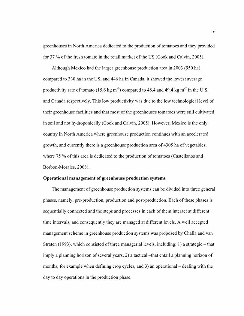
The steps and processes within each of the phases are further detailed in Figure 2.
Each component is equally important and the proper management will contribute to the
overall success of the production system. Most decision-making processes are
concentrated in the production phase, where the majority of the management options for
directly or indirectly ‘steering’ the growth, development and plant growth-mode, has
been automated with the advances in computer control technologies.
Pre-production Production Post-Production
Transplanting Harvesting
Tactical management (Crop cycles)
Operational management (daily)
Strategic management (Several years)
18
Greenhouse (Tomato) Production
Pre-production Production Post-production
Long term planning (Years)
Site selection
Greenhouse design
Seasonal planning (months)
Crop selection
Cultivar selection
Production planning
Preparation (seasonal)
Cleaning and disinfecting
Seedling preparation
Management (weekly/daily/minutes)
Shoot environment
Root environment
Crop maintenance
Pest and diseases (IPM)
Air Temperature
Humidity (RH, VPD)
Water
Nutrients (EC, pH, ratios)
CO2
Light (PAR)
Short term planning (weekly/daily)
Cleaning
Sorting
Packing
Storing & Distribution
Marketing
Leaves and side-shoots removal
Fruit pruning
Plant training (clipping, leaning and lowering)
Growth, Development and Plant Health
Figure 2. Overall steps and processes within a greenhouses production system
19
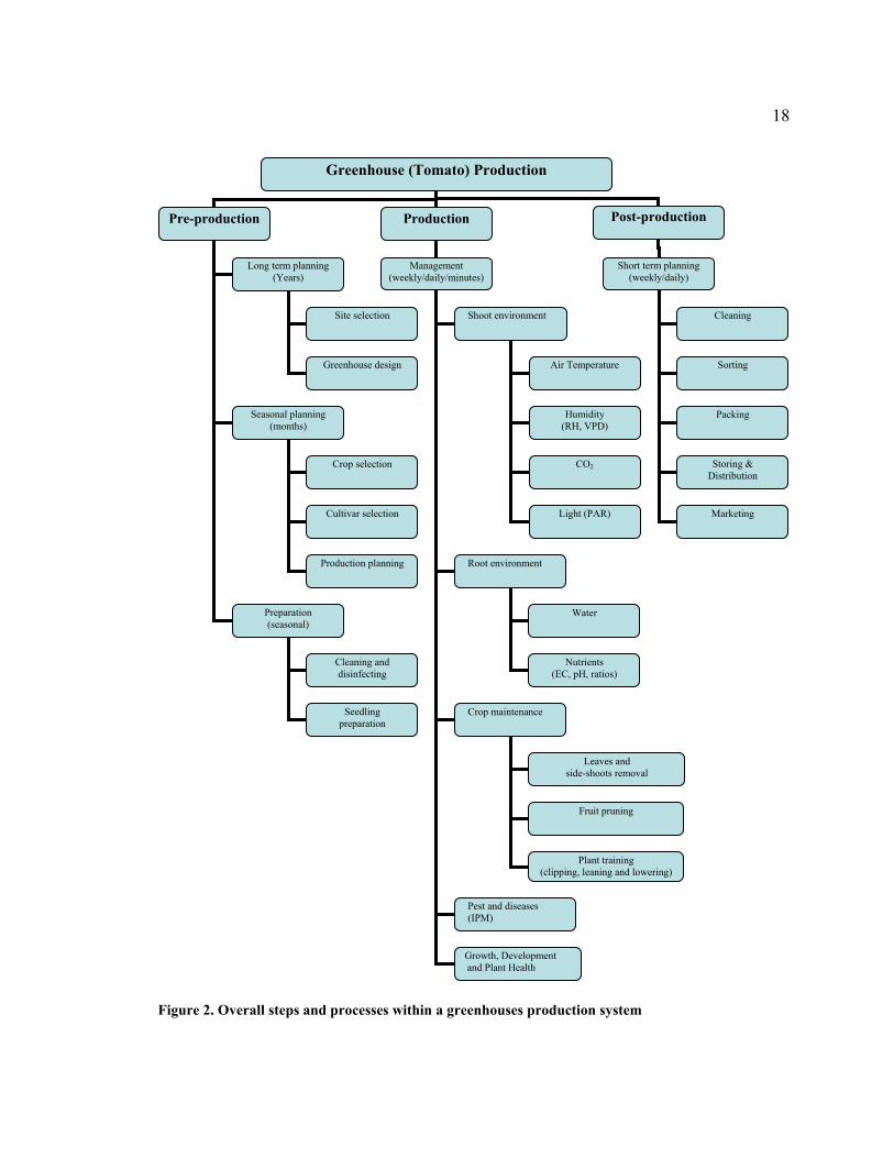
The biophysical (crop-greenhouse) system
The interactions between the biological and physical components of the crop-
greenhouse system are simplified and represented in Figure 3. This representation is
adapted from the one proposed by van Henten and Bontsema , where a hierarchical
decomposition of the optimal greenhouse climate management is proposed to integrate
the slow and fast dynamic response time of the biological and physical components,
respectively.
Figure 3. Diagram of the biophysical (crop-greenhouse) production system
The management of both, the shoot and root environments is highly automated and
consists only of defining the set-points of each of the parameters to be controlled, and
then implementing them with the computer-based climate controller. These parameters in
Greenhouse environment (aerial and root zone)
Crop
Feedback from crop observations and environmental parameters mapped into a set of environmental control actions
External disturbances
20
the shoot environment include: 1) air temperature, 2) humidity, 3) CO2 concentration, and
4) light intensity and quality, and in the root environment, the parameters are: 1)
irrigation frequency, and 2) the nutrients provided as characterized by EC (electrical
conductivity), pH, and dissolved oxygen. These are all of equal importance for
production of a quality crop. However, the management of the other three control
mechanism (pest and disease management, crop maintenance, and growth-mode) for
influencing the growth and development of the crop depend completely on the human
observation and on the experience of the grower for detecting critical information and for
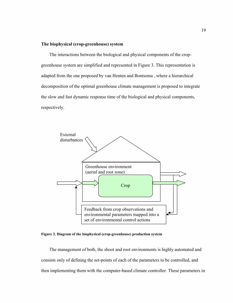
implementing adequate actions. These crop observations are shown in Figure 4 in a
hierarchical way.
Plant Monitoring
Yield (kg m-2 )
Quality: • Fruit size • Fruit disorders • Flavor & • Nutritional content
Developing Time (days from fruit set to harvest)
• Growth • Development • Growth-mode (Reproductive,
Balanced, Vegetative)
Plant Health: • Nutrient deficiencies • Fruit disorders • Diseases
1) Detection level
2) Evaluation level
Figure 4. Crop parameters used as inputs in the decision-making process of the operational management of the biophysical system. These parameters and plant evaluation factors are the biological feedback to adjust the overall system.
21
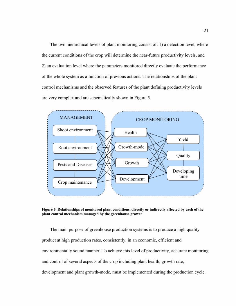
The two hierarchical levels of plant monitoring consist of: 1) a detection level, where
the current conditions of the crop will determine the near-future productivity levels, and
2) an evaluation level where the parameters monitored directly evaluate the performance
of the whole system as a function of previous actions. The relationships of the plant
control mechanisms and the observed features of the plant defining productivity levels
are very complex and are schematically shown in Figure 5.
MANAGEMENT CROP MONITORING
Shoot environment HealthYiel
Figure 5. Relationships of monitored plant conditions, directly or indirectly affected by each of the plant control mechanism managed by the greenhouse grower
The main purpose of greenhouse production systems is to produce a high quality
product at high production rates, consistently, in an economic, efficient and
environmentally sound manner. To achieve this level of productivity, accurate monitoring
and control of several aspects of the crop including plant health, growth rate,
development and plant growth-mode, must be implemented during the production cycle.
Root environment
Pests and Diseases
Crop maintenance
Growth-mode
Growth
Development
d
Quality
Developing time
22
The desired features of a healthy, productive and balanced crop are achieved by
controlling: 1) the shoot environment, 2) the root environment 3) adequate crop
maintenance, 4) pests and diseases, and 5) the plant growth-mode, to optimum levels
appropriate for the stage of the crop, season of the year and current objectives for the
crop by the grower.
The two main plant control mechanisms, directly affecting the physiological
processes, and ultimately affecting the growth, development and plant growth-modes are:
1) the shoot environment where the factors controlled by the climate control system are
the air temperature, humidity, carbon dioxide (CO2) concentration, and solar radiation;
and 2) the root environment where the frequency and timing of the irrigation and supply
of nutrients are controlled by the nutrient delivery (hydroponic) system. Both of these
environments are automatically controlled, by following preset values, ‘set-points’, on
each of the environmental parameters.
The “optimum” environmental conditions have been heuristically determined and
defined by experienced growers and researchers through many years of crop production
and experimentation. Today these optimum conditions are successfully achieved at a
reasonable accuracy by implementing crop-specific blueprints for the manipulation of
several actuators (exhaust fans, ventilation openings, shade curtains, heaters, boilers,
water pumps, etc.) with basic control strategy to reach desired set-points.
With the advancements of computer technologies it has become possible to
simultaneously monitor and control several environmental parameters, and to implement
more sophisticated control techniques, including hierarchical control techniques that
23
solve the problem of the slow and fast dynamic responses of the biological and physical
components in the coupled crop-greenhouse system (van Henten and Bontsema, 1996).
These control schemes depend on mathematical models for describing the dynamics of
the coupled crop-greenhouse system, and to adjust set-points dynamically to optimize
crop growth for a given performance criterion (Seginer, 1993; van Straten et al., 2000).
Despite the technological advances and the sophistication of greenhouse hydroponic
and climate control systems, greenhouse operations primarily rely on human expertise to
decide and to adjust the appropriate optimum values for each of the production and
environmental parameters in the crop-greenhouse system, and most importantly, to verify
by observation the desired response of the crop. Besides the environmental control, the
three other mechanisms also influencing growth and development of the crop depend
completely on the human experience for detecting and properly implementing an action.
These mechanisms include: 1) proper crop maintenance (for tomato, cucumber and sweet
pepper, include deleafing, removing side shoots, fruit pruning, plant training, etc.), 2)
prompt identification and control of pests and diseases, and 3) balancing of the growth-
mode by maintaining appropriate biomass source-sink proportion.
24
PROBLEM STATEMENT
Greenhouse production systems are very complex and their operation requires
managing multiple critical processes simultaneously throughout the production cycle.
The overall task of greenhouse management consists of selecting the appropriate sets of
actions that will provide optimum productivity levels given the present conditions of
external factors and the current status of the crop. These actions will directly affect the
aerial and root zone environments and indirectly affect the crop status, plant health and
productivity.
A successful greenhouse production system begins with the proper selection of
actions at each of the managerial levels. For example, at the strategic level, the location
of the greenhouses are defined according to the needs of the crop to be grown, and to the
availability of water, land, roads, energy, markets, and labor supply (Nelson, 2003). In
the same way the greenhouse design, the orientation and the layout are properly defined
according to climate conditions and crop needs (Giacomelli, 1989). Many greenhouse
crop production systems have failed from the beginning due to the choices implemented
during the strategic planning phase. On the other hand, many other production systems
have failed during operational management due to the lack of experience to promptly
identify problems and implement corrective actions, or to properly assess the current
status of the crop which drives the decision-making process for adjusting the overall
system.
The subjective nature of observing each of the plants responses, indirectly affect the
decision-making process for selecting the ‘optimum’ set of actions to induce a growth
25
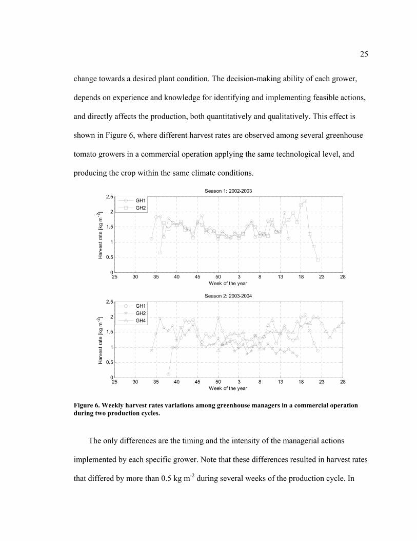
change towards a desired plant condition. The decision-making ability of each grower,
depends on experience and knowledge for identifying and implementing feasible actions,
and directly affects the production, both quantitatively and qualitatively. This effect is
shown in Figure 6, where different harvest rates are observed among several greenhouse
tomato growers in a commercial operation applying the same technological level, and
producing the crop within the same climate conditions.
25 30 35 40 45 50 3 8 13 18 23 280
0.5
1
1.5
2
2.5
Week of the year
Har
vest
rate
[kg
m -2
]
Season 1: 2002-2003
25 30 35 40 45 50 3 8 13 18 23 280
0.5
1
1.5
2
2.5Season 2: 2003-2004
Week of the year
Har
vest
rate
[kg
m -2
]
GH1GH2
GH1GH2GH4
Figure 6. Weekly harvest rates variations among greenhouse managers in a commercial operation during two production cycles.
The only differences are the timing and the intensity of the managerial actions
implemented by each specific grower. Note that these differences resulted in harvest rates
that differed by more than 0.5 kg m-2 during several weeks of the production cycle. In
26
addition, the differences in production actions probably caused dissimilar resource
(energy, water, CO2 consumption, gas, labor, etc.) usage as well.
These weekly productivity variations may seem insignificant, but when they occur
within large commercial operations they can be enormous, as their impact is proportional
to the production area which may be tens to hundreds of hectares. Besides the direct
impact on the revenues, the variations affect the management of resources, such as labor,
energy, gas, water, etc., and ultimately the marketing strategies that can be implemented.
In addition, increased and consistent production capability can eliminate the requirement
for construction of more greenhouse systems, thereby reducing capital investments.
The economic impact as a function of production area and harvest rate variations is
shown in Figure 7. Assuming a sales value of $1.0 kg-1 and a production area of 100 ha, a
small harvest rate variation of 100 g per square meter within a week represents 100,000
dollars per week, or 3.5 million dollars on a 35 weeks average production cycle. The
observed yield variation among growers in Figure 6 was of more than 500 g during
several weeks, which is directly proportional to the production area managed by each
grower.
The decision-making process in the operation of a greenhouse production system
starts with gathering descriptive information about the status of the crop-greenhouse
system, then, evaluating alternative actions and foresee their responses, and finally
selecting and implementing a set of actions appropriate for the actual condition. Having
an integral system capable of controlling and implementing the decision-making process
in each of the phases and steps of production is nearly impossible. Several decision

27
support systems (DSS) for specific plant processes in the operational management have
been proposed in the past and they will be discussed in the literature review.
0 20 40 60 80 100 1200
100
200
300
400
500
600
Production area [ha]
Tota
l yie
ld v
aria
tion
per w
eek
(x 1
000)
[kg
wee
k -1]
0.1 [kg m-2 week-1]0.20.30.40.5
Figure 7. Total yield variation per week as a function of production area and several harvest rates differences.
Greenhouse production systems have become the alternative production practice to
satisfy the consumer demand of healthier, safer and higher quality produce in a year-
round manner, while implementing environmentally friendly methods that make efficient
use of resources such as land, water, labor, capital and energy. However, they are highly
dependent on energy, skilled labor, effective management and increased knowledge of
growing specific crops (Giacomelli et al., 2007; Jensen, 2002).

28
In its most advanced technological level, greenhouse production systems are highly
capital intensive and a technologically demanding agricultural practice, which has come
to rely more on computer-based technologies for monitoring the plant environment,
organizing and evaluating plant response to the environment, and for making accurate
and informed decisions about the crop management within the different time scales,
ranging from hourly, daily, weekly, seasonally, to yearly for controlling each of the
processes in the production cycle.
Several computational systems implementing mechanistic and intelligent algorithms
were proposed for supporting the decision-making process at the strategic, tactical, and
operational managerial aspects for greenhouse tomato production. Although the tomato
crop was used in the implementation, the resulting systems could be adapted to other
greenhouse crop of long production cycles, such as cucumbers and sweet peppers.
29
LITERATURE REVIEW
Mechanistic and empirical models of the biophysical system
The relationships between the plant control mechanisms and the biological processes
in the plants have been modeled through mechanistic and empirical models with the
purpose of finding the proper set of actions that produce desired plant features. The
results of the models had been useful to increase the understanding of each of the
individual dynamic processes either in the plants, in the greenhouse environment, or
partially in integrated crop-greenhouse models.
Plant-based models
Tomato crop growth is a dynamic and complex phenomenon and it has been studied
through the development of mechanistic and empirical models for greenhouse tomato
crops. The two most complex and complete mechanistic models that describe the
dynamic growth of greenhouse tomato plants are TOMGRO (Jones et al., 1991; Jones et
al., 1999) and TOMSIM (Heuvelink, 1996; Heuvelink, 1999). Both models were based
on plant physiological processes of photosynthesis and maintenance respiration, and
model biomass partitioning, determining growth and yield of dry mass as a function of
climate conditions and plant physiological parameters. Their use has been limited for
practical application by growers, because of their complexity and by the difficulty to
obtain the model initial condition parameters required for implementation (Challa and
Heuvelink, 1996). However, the models have been important tools for developing the
30
theoretical foundation of the dynamic response of the biological component of the
greenhouse system.
Many plant-oriented models were developed to understand the effects on the growth,
development and yield in tomato plants under specific controlled environmental
conditions, such as, air temperature (Heuvelink, 1989), light intensity levels (Bruggink
and Heuvelink, 1987), atmospheric humidity (Bakker, 1991; Jolliet, 1994; Jolliet and
Bailey, 1992), and CO2 concentration (Willits and Peet, 1989). They have been used to
define the range of optimum environmental parameters for enhanced plant productivity.
Other models have focused on specific plant processes such as transpiration of
greenhouse crops (Stanghellini, 1987), as effected by VPD (Leonardi et al., 2000) or EC
(Li and Stanghellini, 2001), and the effect that they have on vegetative growth and the
quality of fruit yield in tomatoes.
Other plant-oriented models focused on the effects of crop maintenance practices
(labor) on the production rate and quality of the fruit yields. Crop maintenance practices
include the labor necessary for fruit pruning, which directly affects the fruit load and
ultimately the dry matter partitioning (Heuvelink, 1997), as well as, side shoot and leaf
removal which directly affect the overall crop canopy net photosynthesis (Acock et al.,
1978), and ultimately the supply of photosynthetic assimilates which affect growth, and
fruit yield (Heuvelink, 1995; Heuvelink, 1996)
Recent plant-oriented models have focused on the effect of specific pest and diseases
on plant growth and yield (Boulard, 2007; Tantau and Lange, 2003). The plant-oriented
models have helped to define the bounds of optimum plant growth and productivity. To

31
achieve the optimum environmental conditions the physics of the greenhouse must be
completely understood to implement the required environmental control strategies,
utilizing the available environmental control systems.
Greenhouse-oriented models
The “optimum” environmental conditions have been heuristically determined and
defined by growers and researchers through many years of experimentation, and today
these optimum conditions are successfully achieved by implementing simple on-off
control on the actuators which use set-points as reference points for activation. However,
with the advancements of computer technologies it has become possible to monitor and
control multiple parameters simultaneously, and to implement sophisticated control
techniques, which are based on modern control theories. These control schemes depend
on mathematical models, describing the dynamics of the coupled crop-greenhouse system,
to dynamically adjust set-points to optimize crop growth for a given performance
criterion (Seginer, 1993; van Straten et al., 2000).
Several greenhouse models, based on energy and mass balance equations, have been
investigated in the past and they can be classified as static or dynamic models (Stanhill
and Enoch, 1999). The more complex models are coupled with the crop dynamics (Jones
et al., 1988; Jones et al., 1990; Takakura et al., 1971), and they include several state
variables describing the status of the system over time. Some models were focused on
specific environmental control methods, for example, natural ventilation (Al-helal, 1998;
Boulard and Draoui, 1995; Boulard et al., 1999; Dayan et al., 2004; Jong, 1990), forced
32
ventilation (Arbel et al., 2003; Willits, 2003), evaporative cooling (Abdel-Ghany and
Kozai, 2006; Baille et al., 1994; Boulard and Baille, 1993; Boulard and Wang, 2000), or
heating systems (Bartzanas et al., 2005; Kempkes et al., 2000).
Greenhouse-oriented models with optimization principles
Newer research approaches for greenhouse climate control are based on optimization
principles, for example, for decreasing energy (Aaslyng et al., 2003; Körner, 2003; Zwart,
1996), and water (Blasco et al., 2007) consumption; for optimizing CO2 usage (Jones et
al., 1989; Linker et al., 1998; Seginer et al., 1986), or humidity control (Daskalov et al.,
2006; Jolliet, 1994; Korner and Challa, 2003; Stanghellini and van Meurs, 1992). Other
climate control studies implemented different types of control criteria, such as, economic-
based optimal control (Tap, 2000; van Henten, 1994), adaptive control (Udink ten Cate,
1983), multi-objective hierarchical control (Ramirez-Arias, 2005), or nonlinear predictive
control (El-Ghoumari, 2003).
Greenhouse production systems have a complex dynamic which is driven by external
factors (weather), influenced by control mechanisms (ventilation openings, exhaust fans,
heaters, evaporative cooling systems, etc.) and by the physiological processes of the crop
(transpiration). Thus as the physics of the greenhouse environment is better understood,
the greenhouse design and component selection will be enhanced such that the
greenhouse production system will have improved probably for success and improved
operational performance.
33
Decision-making in greenhouse production systems
Experienced greenhouse tomato growers and researchers assess plant responses and
growth-modes, based on real-time visual observations of plants morphological features.
They use this information for making decisions on climate control and crop management
practices to grow the plant for optimum results. The long-term goal is to direct the plant
growth towards a “balanced” growth-mode with appropriate proportion of vegetative
mass to support the existing fruit load, and appropriate proportion of fruit load to
maintain desired yield and fruit quality. Morphological observations include both
quantitative (length, diameter, and elongation rates, etc.) and qualitative (shape, color,
texture) features of the plant growing tip (head), stem, number of flowers and fruits,
trusses, and leaves (Jensen, 2004; Papadopoulos, 1991; Portree, 1996).
The decision-making (DM) process is a human activity that has been analyzed under
several frameworks. DM is a sequential and continuous process which includes a set of
phases and step activities. Table 1 includes a summary of the phases and steps on the
decision-making process proposed by Mora et al. (2003) and adapted to greenhouse
environment management.

34
Table 1. Decision-making phases and steps for management of greenhouse production systems. Adapted from Mora et al. (2003) Phases Steps Descriptions applied to greenhouse management
Data gathering Observe the qualitative and quantitative morphological features of the plant defining its growth-mode, and current and historical greenhouse climate data.
Intelligence
Problem recognition
Interpret collected data, by assessing the plant growth-mode, and overall health of the crop.
Model Formulation
Determine possible growth-mode imbalances, and problems with growth and development, and any other possible plant symptom (nutrient deficiencies, diseases, etc.)
Design
Model Analysis Define set of actions to steer the growth-mode to the proper level. (Increase or decrease air Temperature, humidity levels, CO2 concentrations, Irrigation frequencies, etc.)
Generation and Evaluation
Evaluate a set of actions most adequate to the current objectives
Choice
Selection Choose the optimum set of actions Result presentation
Translate actions into controllable options (set points) for each parameter to control.
Task planning Schedule the implementation of new set-points
Implementation
Task tracking Observe if the new adjustments are properly implemented (in the physical environment). Observe plant response in the next few days. (a new reality)
Outcome process analysis
Record control strategies associated with plant responses
Learning
Synthesis Communicate and discuss strategies with other growers.
As information technologies have evolved, decision support systems (DSS) have
developed from simple computational tools used to gather, store and access and report
information, into complex analytical tools that add creativity, robustness and intelligence
to the decision-making process. These information systems can be categorized as DSS,
executive information systems (EIS), artificial intelligent systems (AIS), knowledge-
35
based systems (KBS), machine learning system (MLS), and intelligent decision support
systems (IDSS), which is a combination of DSS and MLS. Many others are defined
according to the architecture and the inference mechanism for decision-making
(Forgionne, 2002). When decision support systems integrate several computerized
support tools to directly or indirectly support all the phases of the decision-making
process, they are collectively called Decision-Making Support Systems (DMSS). The
decision-making process is usually implemented for recognizing or diagnosing a problem
and then searching for a solution, or it may be used for identifying an opportunity and
seizing on the potential benefits.
In the case of greenhouse production management, several types of DSS have been
reported in the literature to enhance the decision-making process for each of the
managerial tasks. For example Ting et al. (1993) developed a DSS for single truss tomato
production, focusing on the processes of the production planning (scheduling production,
calculating plant densities and sizing seedling areas, calculating space utilization
efficiencies, calculating labor requirements and predicting yield and revenues).
A more integral DSS aimed to support the operational management of several
processes in low technology greenhouse for the cultivation of six vegetable crops,
including tomato, was the one proposed by Passam et al. (1997). This system integrated:
1) a diagnostic expert system (DES) for managing the most common pests, diseases and
nutritional deficiencies, 2) a control expert system (CES) for managing irrigation and
fertilization, 3) an information presentation package to provide decision support at the

36
tactical managerial level, and 4) a market presentation module to provide decision
support for the packaging and market presentation of produce.
Another suite of DSS tools were integrated in the Harrow Greenhouse Manager
(HGM) which includes a knowledge base for the management of pest and disease, and
general information for the production of greenhouse cucumbers and tomatoes (Clarke et
al., 1999)
Many other DSS reported in the literature, were focused on one component, or one
particular process, within the whole spectrum of processes in greenhouse production
systems. For example, there were DSS for managing the root environment, either
supporting the management of plant nutrition (Fynn et al., 1994; Fynn et al., 1989) or
irrigation under several conditions, in soilless cultures including saline conditions
(Ferentinos et al., 2003), or in closed loop irrigation (Bar-Yosef et al., 2004).
Other DSS attempted supporting the management of the shoot environment and
implemented different decision-making methodologies, such as KBS (Schotman, 2000)
and simple DSS of physical environment models (Chandra and Dogra, 2002; Schmidt,
2004), or proposed new greenhouse climate management paradigms, such as, the
dynamic daily generation of optimal set-points (Tchamitchian et al., 2006) or the
dynamic generation of climate control strategies based on temperature integration and the
DIF concept (Korner and Van Straten, 2008) for energy saving.
Greenhouse production systems face new challenges imposed by competitive
international markets, by new regulation on the use of chemicals, by the increased
consumer demand for healthier, safer, more nutritious, and eco-friendly products, by the

37
increasing energy costs for production and transportation, and by the increased concern
of making efficient use of resources (energy, land, water, and labor) to have a sustainable
production system. All these challenges add additional complexity to the already complex
system. It is evident that new tools to support the decision-making process under these
new challenges are required. Decision support tools that implement computational
intelligence techniques, such as, neural networks, fuzzy logic, genetic algorithms,
knowledge-based system, etc. are an alternative for these type of problems (Kamp and
van der Veen, 2002; Martin-Clouaire et al., 1996).
Intelligent decision support systems in greenhouse production systems
Intelligent decision support systems (i-DSS) extend the traditional DSS capabilities
by incorporating one or more computational intelligent techniques which could add
learning and reasoning capabilities (neural networks), or allow the incorporation of
specific domain knowledge (expert knowledge) in a quantitative and qualitative way
(fuzzy logic). A i-DSS must be able to include learning and reasoning capabilities,
elaborate and evaluate decision alternatives and specify relationships between criteria,
alternatives, events and choices (Phillips-Wren et al., 2006). The only known-to-date true
i-DSS applied in greenhouse production systems was SERRISTE (Tchamitchian et al.,
2006), which generated daily climate set-points for greenhouse tomato production. This
system incorporated crop management knowledge, derived from scientific research and
from expert growers, as a constraint satisfaction problem using fuzzy logic.
38
Computational intelligent techniques have been applied in many greenhouse plant
production applications, either for modeling or for controlling a specific process.
However these are not considered as decision support systems, because they describe
only one process and do not have the ability to simulate different scenarios or do not offer
the ability of interaction. Most of the reported applications are concentrated in the physics
of the greenhouse. Following is a brief description of the two most implemented
computational intelligent techniques in greenhouse plant production.
Neural networks on greenhouse systems
Computational neural networks are mathematical representations of the way
biological neurons process information as parallel computing units. They have proved to
be a powerful tool to solve several types of problems in different fields where
approximation of nonlinear functions, classification, identification and pattern
recognition were required. In general there are two types of neural network architectures:
1) static (feedforward), where no feedback or time delays exists, and 2) dynamic neural
networks, whose outputs depend on the current, or previous inputs, outputs or states of
the network (Demuth et al., 2007). One of the most widely used neural network
architectures is the multilayer perceptron (MLP), which has been proved to approximate
almost any continuous function over a compact subset of Rn, if given enough hidden
layers and neurons within them (Master, 1993). A MLP is a structure mapping an input
space Rn into an output space Rm, by adjusting the connection weights, linking each of the
input elements to the neurons in the hidden layers and throughout the output layer.
39
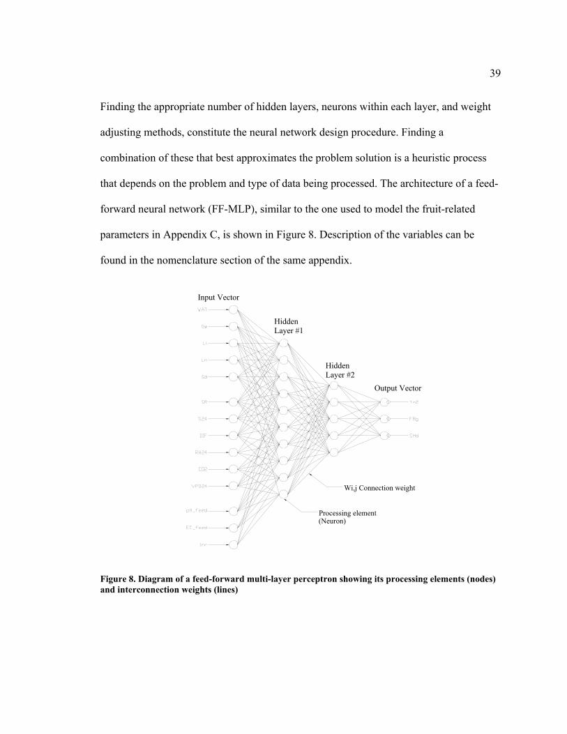
Finding the appropriate number of hidden layers, neurons within each layer, and weight
adjusting methods, constitute the neural network design procedure. Finding a
combination of these that best approximates the problem solution is a heuristic process
that depends on the problem and type of data being processed. The architecture of a feed-
forward neural network (FF-MLP), similar to the one used to model the fruit-related
parameters in Appendix C, is shown in Figure 8. Description of the variables can be
found in the nomenclature section of the same appendix.
Input Vector
Hidden Layer #1
Hidden Layer #2
Output Vector
Processing element (Neuron)
Wi,j Connection weight
Figure 8. Diagram of a feed-forward multi-layer perceptron showing its processing elements (nodes) and interconnection weights (lines)

40
Fuzzy logic on greenhouse systems
Fuzzy logic (FL) is an extended generalization of the classical two-valued logic for
reasoning within uncertainty (Zadeh, 1965). It implements fuzzy sets, which are sets with
un-sharp boundaries, and where notion of membership of a set becomes a matter of
degree. Fuzzy logic offers the advantage of evaluating imprecise data, because it allows
for the implementation of general knowledge (i.e. growers experience) by using a natural
language or linguistic variables through inferences systems capable of dealing with
uncertainty, and where qualitative and quantitative features can be combined to model
complex systems. Fuzzy rule-based models are used in control systems, decision making,
and pattern recognition among many others. Further details of the theory, history and
applications can be found in fuzzy logic references (Buckley and Eslami, 2002; Piegat,
2001; Yen and Langari, 1999).
In greenhouse production systems FL has been applied for modeling (Lanfang et al.,
2000; Salgado and Cunha, 2005) and controlling (Castaneda-Miranda et al., 2006;
Ehrlich et al., 1996) the aerial environment, as well as, to model processes such as
photosynthesis (Center and Verma, 1997) and growth (Weiping and Hanqin, 1988) in
tomato plants.
41
PROJECT OBJECTIVES
The complexity of greenhouse production systems imposed by the non-linear
behavior, the slow or fast time dynamic responses on each of its processes, and the
intrinsic interactions among all the components, results in ill-defined systems which are
difficult to represent in traditional mathematical models that attempt to describe precise
behavior. Although several models can be found in the literature that increase the
understanding by describing, 1) plant specific processes, such as, photosynthesis,
respiration, biomass production and partitioning, plant growth and development, etc., 2)
the physics of the greenhouse environment, and 3) the overall behavior of the coupled
crop-greenhouse system, none are known to have been implemented commercially
(Challa and Heuvelink, 1996; Lentz, 1998).
Despite the technological advances and the sophistication of greenhouse hydroponic
and climate control systems, the day-to-day operation primarily relies on the feedback
from the grower to adjust each of the plant control mechanisms to obtain a desired plant
condition.
Greenhouse management is an intensive decision-making activity in each of the
phases, steps and processes, and the proper combination of actions to manage all the
processes in the production system is important to a successful operation. Experienced
greenhouse managers and researchers assess plant responses and growth-mode, based on
visual morphological observations of the plants. They use this information for managing
the control mechanisms to induce a desired plant status.
42
The subjective nature of the assessment of the performance of the biological
component in greenhouse production systems motivates the development of
computational tools to enhance the decision-making process for the appropriate selection
of actions in managing greenhouse operations. There is an immediate niche for
knowledge-oriented systems to be integrated into the greenhouse production systems at
all three managerial levels and at each of its phases and steps.
Therefore, the overall objective of this study was to develop computational tools to
enhance the decision-making process at the strategic, tactical and operational managerial
level in several processes of greenhouse tomato production systems. The specific
objectives and its correspondent justifications were:
1. To develop and implement a dynamic greenhouse environment model for
simulating the greenhouse environment of user-selected greenhouse
configurations and control strategies under several climatic conditions.
The justification was that the success of greenhouse commercial operations start
with the adequate selection of the site location and with an adequate greenhouse
design configuration that will meet the crop needs and will overcome the climate
conditions. These selections are part of the strategic planning, and having a tool
that allows the evaluation of several alternatives of greenhouse designs and
different climate conditions will improve the decision-making process for the
adequate greenhouse design and optimum location.
2. To establish a Web-based crop monitoring system capable of retrieving
greenhouse climate data in semi-real time and images of the crop in real-time, for
43
purpose of remote diagnosis and analysis.
The justification was that at the operational level, the first step before adjusting
any of the mechanisms of plant manipulation is the assessment of the current
status of the crop-greenhouse system. By increasing the capability of remote
inspection more information and knowledge could be implemented in the proper
assessment and diagnosis of the crop conditions.
3. To characterize the growth-mode (vegetative, balanced, or reproductive) of
greenhouse tomatoes plants with Fuzzy modeling as a function of plant
morphological features currently recorded and utilized by most greenhouse
tomato growers.
The justification was that the growth-mode assessment is part of the day-to-day
operational management. It is a very subjective concept defined by the visual
inspection of quantitative and qualitative plant morphological features. Having a
system that characterizes the growth-mode in a simplified way (with a numerical
scale) by defining the type of growth and its degree, would enhance the decision-
making process for taking the proper set of actions to steer the crop towards a
desired growth-mode.
4. To model and predict fruit-related parameters (harvest rates, fruit size, and fruit
developing time) of greenhouse tomatoes with dynamic neural networks as a
function of current and historical data of the greenhouse environment and plant
morphological features.
The justification was that the overall performance of the greenhouse production
44
system is directly evaluated by the quantity, quality and production time of the
marketable product, in this study, tomatoes. Having a tool that models each of
these features could allow the evaluation of several management alternatives to
achieve a desired production level. In addition the management of other resources
such as labor, energy, water, and marketing strategies could be improved
according to projected productivity levels.
45
DISSERTATION FORMAT
The format of this dissertation follows the Agricultural and Biosystems Engineering
Departmental paper option. The findings on each of the manuscripts are put in the context
of the overall management of greenhouse production system, which is described in the
introduction and general discussion of the project.
In place of chapters, the manuscripts describe self-contained portions of this study.
Following is a general discussion of the main contributions towards the overall
managerial context of greenhouse production systems.
Proposed paper contribution 1: Appendix A. Dynamic modeling and simulation of greenhouse environments under several scenarios: a web-based educational application.
This research was part of broader, multi-institutional (The University of Vermont,
University of Florida, The Ohio State University, and The University of Arizona)
collaborative effort to develop Web-based multimedia instruments for improving
worldwide greenhouse education. The overall project included the development of: 1)
digital videos describing the greenhouse production systems at each location, 2) a
searchable repository of greenhouse educational material including images, videos and
software, 3) an instructor web-based student evaluation method to determine extent of
learned greenhouse concepts, and 4) a greenhouse environment simulator (Tignor et al.,
2006; Tignor et al., 2007). The greenhouse environment simulator that was developed
included a computer simulation program based on a greenhouse environment
mathematical model and was programmed in ActionScript 2.0, and integrated into an
46
interactive interface developed in Flash MX (Flash MX Pro 2004, Macromedia, San
Francisco) (Fitz-Rodriguez, 2006). The components of the simulation program included
climate data, database of greenhouse structure and hardware equipment features, and the
mathematical model representing the physics of the greenhouse and crop environment.
This appendix includes the first objective of the project, which was to develop and
implement a dynamic greenhouse environment model for simulating the environment of
several user-selected greenhouse configurations, control strategies and climatic
conditions.
Several simulations scenarios were conducted to validate the overall performance of
the models. These simulations allowed the comparison of the resulting greenhouse
environment when applying different control strategies, e. g. ventilation rates, heating
and cooling capacities, shading, and different crop sizes.
Specifically, Appendix A provides:
• A dynamic model for simulating the physics of the greenhouse environment.
• An interactive Web-based computational tool that allows the evaluation of diverse
user-selected greenhouse configurations, defined by the structural design, glazing
material, and diverse climate control components.
47
Proposed paper contribution 2: Appendix B. Tomatoes Live! 2.0: A Web-Based Greenhouse Monitoring System
This appendix includes the second objective of the project, which was to develop a
Web-based crop monitoring system for enhancing remote diagnosis. The resulting system
allowed the integration of different vendor-specific greenhouse climate controller and
data recording units implemented in several research greenhouses at the Controlled
Environment Agriculture Center (CEAC) of the University of Arizona.
The off-site monitoring of the crop-greenhouse system removed the spatial and
temporal limitations of current climate controllers, and allowed for the continuous
monitoring of the system status at the operational management level. By extending the
accessibility of information related to the current and past condition of the production
system, the decision-making process could be enhanced through remote diagnosis from
experts not locally available.
Specifically, Appendix B provides:
• An information system to extend the monitoring capabilities of the greenhouse
environment and direct plant observation with the use of Internet technologies.
• A systematic way for gathering data from different vendor-specific greenhouse
climate controllers and data recording units.
• Homogenized raw data to create grower-specific multi-factor parameters for
consistent comparison among multiple production units.
• Algorithms to process data and compute plant-oriented parameters
48
Proposed paper contribution 3: Appendix C. Yield prediction and growth-mode characterization of greenhouse tomatoes with neural networks and fuzzy logic
This appendix includes the third and fourth objectives of the project which were to
develop computational intelligent models to characterize plant growth-mode and to
predict yield, quality and production time in commercial greenhouse tomato production
systems. The ability to predict the outcomes of the system as a function of current and
historical data of climate and plant parameters is directly applicable in the operational
management to evaluate different control strategies. The data used for designing, training
and evaluating these computational intelligent models were derived from greenhouse
operations at the CEAC research facilities, and at a commercial greenhouse operation.
Specifically, this Appendix C provides:
• A fuzzy model to characterize plant growth-mode (vegetative, balanced, or
reproductive) as function of plant morphological observations (stem diameter and
distance to the first flower from the apical meristem).
• A dynamic neural network model to accurately predict yield, fruit size, and fruit
development time as a function of parameters (environmental and plant
morphology) currently recorded by greenhouse growers.
49
PRESENT STUDY
OVERALL SUMMARY
The contributions of this dissertation are included in three manuscripts, each in a
separate appendix. Each manuscript includes an introduction, methods, results and
conclusions. The following is a summary of the most important findings in each of the
manuscripts.
DYNAMIC MODELING AND SIMULATION OF GREENHOUSE ENVIRONMENTS UNDER SEVERAL SCENARIOS: A WEB-BASED EDUCATIONAL APPLICATION (APPENDIX A)
The primary objective of this study was to develop and implement a dynamic
greenhouse environment model to simulate the physics of the greenhouse environment
under different user-selected greenhouse configuration, control strategies and climate
conditions.
Currently, greenhouse crop production systems are located throughout the world
within a wide range of climatic conditions. To achieve environmental conditions
favorable for plant growth, greenhouses are designed with various components, and
structural shapes, with numerous types of glazing materials. They are operated differently
accordingly to each condition and crop in production. To improve the decision-making
process on the strategic management, this tool is useful in evaluating different design
configuration and different control strategies for a particular climate condition.
The greenhouse environment model, based on energy and mass balance principles,
was implemented in a Web-based interactive application which allowed for the selection
50
of the greenhouse design, weather conditions, and operational strategies. Several
scenarios were simulated to demonstrate how a specific greenhouse design would
respond environmentally for several climate conditions (four seasons of four
geographical locations), and to demonstrate what systems would be required to achieve
the desired environmental conditions. The greenhouse environment model produced
realistic approximations of the dynamic behavior of greenhouse environments with
different design configurations for 28 hour simulation periods.
Given the amount of choices available through the animated user interface of the
simulator, a staggering number (311,040) of possible scenarios can be replicated, which
makes it helpful as an educational tool for demonstration purposes, and as a decision-
making support tool for appropriate selection of greenhouse configuration and control
strategies in a given climate condition.
TOMATOES LIVE! 2.0: A WEB-BASED GREENHOUSE MONITORING SYSTEM (APENDIX B)
The goal of this study was to develop a Web-based crop monitoring system for
enhancing remote crop diagnosis. The resulting system allowed the integration of
different vendor-specific greenhouse climate controller and data recording units
implemented in several research greenhouses at the Controlled Environment Agriculture
Center (CEAC) of the University of Arizona.
Simple decision-making support tools consist of only information systems capable of
gathering and presenting information in an organized way to help make decision. In this
51
case the monitoring system gathered greenhouse climate data and presents it graphically
in a semi real-time. Also real-time images of the crop were available to make an
assessment of the current state for the crop system.
Knowing the status of the crop-greenhouse system in real time, requires the use of
sensors and controllers for monitoring and controlling each of the environmental
variables. Due to need of environmental control responses to the continually changing
outdoor climate, and the potential failure of the systems within the controlled
environment system, it is valuable to have an information system capable of off-site
monitoring of the greenhouse environment.
The resulting Web-based monitoring system called “Tomatoes Live!” was developed
to oversee greenhouse crop production in educational and research facilities. “Tomatoes
Live! 2.0” (the upgraded version) was accessible to researchers, students and the general
public through the Web at http://ag.arizona.edu/ceac/live2/, where an array of web-
cameras provides a visual accounting of the current crop conditions at each unit, while
semi real-time greenhouse environmental data and related plant oriented calculated
parameters were displayed. The system was successfully used since its implementation in
2001, and it has proved to be valuable not only as an educational tool, but also as an
instrument for remote diagnostics.
52
YIELD PREDICTION AND GROWTH-MODE CHARACTERIZATION OF GREENHOUSE TOMATOES WITH NEURAL NETWORKS AND FUZZY LOGIC (APPENDIX C)
The objective for this portion of the study was to develop computational intelligent
models to characterize plant growth-mode and to predict yield, quality and production
time in greenhouse tomato production systems. The ability to predict the outcomes of the
system as a function of current and historical data of climate and plant parameters is
directly applicable in the operational management to evaluate different control strategies.
Data from greenhouse environments and crop records from experimental production,
located in Tucson, AZ., and from a large scale commercial operation, located in Marfa,
TX., were used for modeling the growth-mode of tomato plants with fuzzy logic. Data
from the commercial operation were implemented to model weekly fluctuations of
harvest rate, fruit size and fruit developing time with dynamic neural networks (NN).
The NN models accurately predicted weekly and seasonal fluctuations of the fruit-
related parameters, having correlation coefficients (R) of 0.96, 0.87 and 0.94 respectively
for harvest rate, fruit fresh weight and fruit developing time, when compared with a
dataset used for independent validation. The fuzzy modeling of growth-mode allowed the
discrimination of reproductive and balanced growth-modes in the experimental systems,
and the seasonal growth-mode variation on the commercial applications. Both modeling
results are applicable to commercial operations for making decisions on greenhouse
climate control and overall crop management practices.
53
OVERALL CONCLUSIONS AND RECOMMENDATIONS
The four decision support systems presented in this study work independently and
potentially enhance the decision-making process at different managerial levels. The first
DSS, which included a dynamic greenhouse environment simulator, was to support the
decision-making process at the strategic and tactical managerial level. The three other
DSS were to support the decision-making process at the operational level. These included
a DSS for real-time monitoring of the overall biophysical system, an i-DSS for
characterizing systematically the plant growth-mode with a limited number of
morphological features (Sd, stem diameter and Th, truss height), and finally an i-DSS for
accurately predicting fruit-related variables (Ya, harvest rate, FRg, fruit size and SHd, fruit
growth period) as a function of current and past condition of the plants and the
environmental strategies implemented (aerial and root zone).
The potential impact and recommendations from each of the DSS proposed are
discussed.
1) At the strategic and tactical managerial level, the greenhouse environment
simulator DSS would improve the decision-making process for selecting an adequate
greenhouse configuration, location, and crop production cycle. This DSS was based on
the dynamic simulation of the greenhouse environment given by a set of greenhouse
configurations and outside climate conditions selected by the user. The capability of
evaluating several greenhouse configurations under several climate conditions,
potentially allowed for a selection of an optimal greenhouse design for the long term and
for the implementation of optimal climate control strategies throughout the production
54
cycle. A better resource planning could be projected given by the variable resource
(energy, water, labor, etc.) utilization throughout the year imposed by the changing
outside climate conditions and by the dynamic changes of international markets. The
flexibility of the DSS to evaluate several scenarios (more than 300 000) over a Web-
based interface, added an educational component useful not only at the college
educational level, but also in extension. Greenhouse managers and small greenhouse
growers could use it for enhancing the understanding of the basic principles of the
physics of the greenhouse environment, and also for evaluating several climate control
strategies. Although this DSS is limited to sixteen outside climate conditions imposed by
four geographic locations (AZ, FL, OH, and VT) and four seasons (spring, summer, fall,
and winter), it could be further improved by including a wider database of greenhouse
configurations, glazing materials and components, and also for allowing the input of new
outside climate conditions. These new features would increase the applicability and
potentially simulate infinite scenarios of greenhouse configurations and control strategies.
2) The DSS for real-time monitoring of the overall biophysical system consisted of a
crop monitoring system which automatically gathers, process and presents greenhouse
environmental data and plant images in real-time with accessibility through the Web,
which increases the capability for remote diagnosis. By increasing the capabilities of
remote diagnosis, the feedback from the current status of the biological component to
adjust the overall biophysical system is further improved by increasing the potential
outreach for expertise of consultants, scientist and educators to adequately assess the
current crop status. Although most of the variables in the aerial and root zone
55
environments are monitored and controlled automatically by computers, the plant
morphological features currently rely on the observations and manual recordings from the
grower. This subjective process continues requiring the grower’s expertise.
The records of the crop morphological features are key components in the final two
i-DSS for modeling fruit-related variables and for characterizing plant growth-mode. The
crop monitoring system not only oversees the performance of the biophysical systems,
but also allows for the detection of failures in the physical components by reviewing
historical data and detecting off-optimum values in the variables of interest.
3) At the operational management level the third DSS proposed potentially improves
the characterization of the plant growth-mode by reducing the number of morphological
features implemented (Sd, stem diameter and Th, truss height), and by reducing the
subjective nature of the assessment. The proposed i-DSS not only characterized the
growth-mode, but also assigned a degree of membership to this feature by implementing
fuzzy logic. The proper assessment of the growth-mode helps to assure the appropriate
adjustment of the overall biophysical system. If an out of balance growth-mode is
detected, a set of actions must be taken in order to induce the proper growth-mode
according to the objectives of production. These sets of actions include the adjustments of
set-points of environmental variables that will induce the desired plant response.
Immediate improvement could increase the applicability of this i-DSS if the two
parameters (Sd and Th) used as inputs were automatically measured. The inputs could be
provided automatically into the i-DSS for real-time assessment of the plant growth-mode.
The system could also be enhanced by defining a universe of sets of actions to induce
56
growth-modes, and include an inference system that would map the set of actions into a
set of set-points for the actuators adjusting the environmental variables.
4) The last i-DSS would enhance the decision-making process at the operational
management level by predicting yield, fruit size and fruit developing time as a function of
current and past conditions of the plants and the environmental strategies implemented.
This i-DSS was derived from full production cycles at a standard commercial tomato
facility, increasing the prediction capabilities of the fruit-related variables, which
included a wide range of plant growing conditions. Several environmental and crop
management strategies could be evaluated to select optimum set of actions resulting in
desired plant productivity.
Similar to the previous i-DSS, this system could be improved by automatically
providing the plant morphological features needed in the dynamic neural network model.
These features could be automatically measured, although it represents a challenge, with
image processing for identifying each of the morphological variables.
The four DSS were described independently to enhance the DM process at each
managerial level. However, they could be linked together to predict year-round
productivity given by a set of environmental and crop management strategies, and
potentially evaluate production costs.
57
REFERENCES
Aaslyng, J.M., J.B. Lund, N. Ehler, and E. Rosenqvist. 2003. IntelliGrow: a greenhouse component-based climate control system. Environmental Modelling & Software. 18: 657-666.
Abdel-Ghany, A.M.and T. Kozai. 2006. Dynamic modeling of the environment in a naturally ventilated, fog-cooled greenhouse. Renewable Energy. 31: 1521-1539.
Acock , B., D.A. Charles-Edwards, D.J. Fitter, D.W. Hand, L.J. Ludwig, W. Warrent, J., and A.C. Withers. 1978. The contribution of leaves from different levels within a tomato crop to canopy net photosynthesis: An experimental examination of two canopy models. J. Exp. Bot. 29: 815-827.
Al-helal, I.M. 1998. A computational fluid dynamics study of natural ventilation in arid region greenhouses. Ph.D. Thesis, The Ohio State University, Columbus, Ohio.
Arbel, A., M. Barak, and A. Shklyar. 2003. Combination of forced ventilation and fogging systems for cooling greenhouses. Biosystems Engineering. 84: 45-55.
Baille, M., A. Baille, and J.C. Laury. 1994. A simplified model for predicting evapotranspiration rate of nine ornamental species vs. climate factors and leaf area. Scientia Horticulturae. 59: 217-232.
Bakker, J.C. 1991. Analysis of humidity effects on growth and production of glasshouse fruit vegetables. Ph.D. Thesis, Wageningen Agricultural University, Wageningen.
Bartzanas, T., M. Tchamitchian, and C. Kittas. 2005. Influence of the heating method on greenhouse microclimate and energy consumption. Biosystems Engineering. 91: 487-499.
Bar-Yosef, B., S. Fishman, and H.P. Klaring. 2004. A model-based decision support system for closed irrigation loop greenhouses. Acta Hort. (ISHS). 654: 107-121.
Blasco, X., M. Martinez, J.M. Herrero, C. Ramos, and J. Sanchis. 2007. Model-based predictive control of greenhouse climate for reducing energy and water consumption. Computers and Electronics in Agriculture. 55: 49-70.
Boulard, T. 2007. Greenhouse-crop system control for a sustainable plant production. Acta Hort. (ISHS). 761: 503-511.
58
Boulard, T.and A. Baille. 1993. A simple greenhouse climate control model incorporating effects of ventilation and evaporative cooling. Agricultural and Forest Meteorology. 65: 145-157.
Boulard, T.and B. Draoui. 1995. Natural ventilation of a greenhouse with continuous roof vents: measurements and data analysis. Journal of Agricultural Engineering Research. 61: 27-36.
Boulard, T., R. Haxaire, M.A. Lamrani, J.C. Roy, and A. Jaffrin. 1999. Characterization and modelling of the air fluxes induced by natural ventilation in a greenhouse. Journal of Agricultural Engineering Research. 74: 135-144.
Boulard, T.and S. Wang. 2000. Greenhouse crop transpiration simulation from external climate conditions. Agricultural and Forest Meteorology. 100: 25-34.
Bruggink, G.T.and E. Heuvelink. 1987. Influence of light on the growth of young tomato, cucumber and sweet pepper plants in the greenhouse: Effects on relative growth rate, net assimilation rate and leaf area ratio. Scientia Horticulturae. 31: 161-174.
Buckley, J.J.and E. Eslami. 2002. An introduction to fuzzy logic and fuzzy sets. Physica-Verlag.
Castaneda-Miranda, R., J. Ventura-Ramos, Eusebio, R. del Rocio Peniche-Vera, and G. Herrera-Ruiz. 2006. Fuzzy Greenhouse Climate Control System based on a Field Programmable Gate Array. Biosystems Engineering. 94: 165-177.
Castellanos, J.Z.and C. Borbón-Morales. 2008. Panorama de la horticultura protegida en Mexico, p. 1-12. In: J.Z. Castellanos (ed.). Manual de producción de tomate de invernadero. INTAGRI, Mexico.
Center, B.and B.P. Verma. 1997. A fuzzy photosynthesis model for tomato. Transactions of the ASAE. 40: 815-821.
Challa, H.and E. Heuvelink. 1996. Photosynthesis driven crop growth models for greenhouse cultivation. Acta Hort. (ISHS). 417: 9-22.
Challa, H.and G. van Straten. 1993. Optimal diurnal climate control in greenhouses as related to greenhouse management and crop requirements, p. 320. In: Y. Hashimoto, G.P.A. Bot, W. Day, and H.J. Tantau (eds.). The computerized greenhouse. Academic Press, New York.

59
Chandra, P.and A.K. Dogra. 2002. A Decision support system for the management of greenhouse environment. Acta Hort. (ISHS). 578: 383-388.
Chikwamba, R., J. McMurray, H.X. Shou, B. Frame, S.E. Pegg, P. Scott, H. Mason, and K. Wang. 2002. Expression of a synthetic E-coli heat-labile enterotoxin B sub-unit (LT-B) in maize. Molecular Breeding. 10: 253-265.
Clarke, N.D., J.L. Shipp, A.P. Papadopoulos, W.R. Jarvis, S. Khosla, T.J. Jewett, and G. Ferguson. 1999. Development of the Harrow Greenhouse Manager: a decision-support system for greenhouse cucumber and tomato. Computers and Electronics in Agriculture. 24: 195-204.
Cook, R.and L. Calvin. 2005. Greenhouse tomatoes change the dynamics of the North American fresh tomato industry USDA Economic Research Report No. 2:86.
Costa, P.and G.A. Giacomelli. 2005. Ensuring success: Protected horticulture production based on levels of technology., Productores de Hortalizas, pp. 48-52.
Daskalov, P.I., K.G. Arvanitis, G.D. Pasgianos, and N.A. Sigrimis. 2006. Non-linear adaptive temperature and humidity control in animal buildings. Biosystems Engineering. 93: 1-24.
Dayan, J., E. Dayan, Y. Strassberg, and E. Presnov. 2004. Simulation and control of ventilation rates in greenhouses. Mathematics and Computers in Simulation
Selected papers of the IMACS/IFAC Fourth International Symposium on Mathematical Modelling and Simulation in Agricultural and Bio-Industries. 65: 3-17.
Demuth, H., M. Beale, and M. Hagan. 2007. Neural network toolbox 5: User's guide. The MathWorks, Inc., Natick, MA.
Ehrlich, H., M. Kühne, and J. Jäkel. 1996. Development of a fuzzy control system for greenhouses. Acta Hort. (ISHS). 406.
El-Ghoumari, M.Y. 2003. Optimización de la producción de un invernadero mediante control predictivo no lineal. PhD, Universidad Autónoma de Barcelona, Barcelona.
Enoch, H.Z.and Y. Enoch. 1999. The history and geography of the greenhouse, p. 1-15. In: G. Stanhill and H. Zvi Enoch (eds.). Greenhouse ecosystems 20. Elsevier.
60
Ferentinos, K.P., A. Anastasiou, D.G. Pasgianos, K.G. Arvanitis, and N. Sigrimis. 2003. A decision support system as a tool to optimal water management in soilless cultures under saline conditions. Acta Hort. (ISHS). 609: 289-296.
Fitz-Rodriguez, E. 2006. Greenhouse environment simulator 1.0: User's manual Vol. 2008.
Forgionne, G.A. 2002. An architecture for the integration of decision making support functionalities, p. 1-19. In: M. Mora, G. Forgionne, and J.N.D. Gupta (eds.). Decision making support systems. Idea Group Publishing, Hershey, PA.
Fynn, R.P., W.L. Bauerle, and W.L. Roller. 1994. Implementing a decision and expert system model for individual nutrient selection. Agricultural Systems. 44: 125-142.
Fynn, R.P., W.L. Roller, and H.M. Keener. 1989. A decision model for nutrition management in controlled environment agriculture. Agricultural Systems. 31: 35-53.
Giacomelli, G.A. 1989. Crop dominated decision-making for greenhouse design. Acta Hort. (ISHS). 257: 183-187.
Giacomelli, G.A. 2004. Engineering design of plant nutrient delivery systems. Acta Hort. (ISHS). 648: 71-81.
Giacomelli, G.A., R.L. Patterson, and P.D. Sadler. 2007. Telepresence technologies and practices for enabling remote semi-autonomous CEA food production. Acta Hort. (ISHS). 761: 21-31.
Heuvelink, E. 1989. Influence of day and night temperature on the growth of young tomato plants. Scientia Horticulturae. 38: 11-22.
Heuvelink, E. 1995. Growth, development and yield of a tomato crop: periodic destructive measurements in a greenhouse. Scientia Horticulturae. 61: 77-99.
Heuvelink, E. 1996. Tomato growth and yield: quantitative analysis and synthesis. Ph.D., Wageningen Agricultural University, Wageningen.
Heuvelink, E. 1997. Effect of fruit load on dry matter partitioning in tomato. Scientia Horticulturae. 69: 51-59.
61
Heuvelink, E. 1999. Evaluation of a dynamic simulation model for tomato crop growth and development. Ann Bot. 83: 413-422.
Jensen, M.H. 2002. Controlled environment agriculture in deserts, tropics and temperate regions -A world review. Acta Hort. (ISHS). 578: 19-25.
Jensen, M.H. 2004. Steering your tomatoes towards profit. Greenhouse Crop Production and Engineering Design Short Course, Tucson, AZ, January 18-21, 2004. p. 3.
Jensen, M.H.and A.J. Malter. 1995. Protected agriculture: A global review. World Bank Technical Paper No. 253.
Jolliet, O. 1994. HORTITRANS, a model for predicting and optimizing humidity and transpiration in greenhouses. J. agric. Engng. Res. 57: 23-37.
Jolliet, O.and B.J. Bailey. 1992. The effect of climate on tomato transpiration in greenhouses: measurements and models comparison. Agricultural and Forest Meteorology. 58: 43-62.
Jones, J.W., E. Dayan, L.H. Allen, H. van Keulen, and H. Challa. 1991. A dynamic tomato growth and yield model (TOMGRO). Transactions of the ASAE. 34: 663-672.
Jones, J.W., E. Dayan, P. Jones, Y. Hwang, and B.K. Jacobson. 1988. Modeling tomato growth for greenhouse environment control. International winter meeting of the ASAE, Chicago, IL.
Jones, J.W., E. Dayan, H. van Keulen, and H. Challa. 1989. Modeling tomato growth for optimizating greenhouse temperatures and carbon dioxide concentrations. Acta Hort. (ISHS). 248: 285-294.
Jones, J.W., A. Kening, and C.E. Vallejos. 1999. Reduced state-variable tomato growth model. Transactions of the ASAE. 42: 255-265.
Jones, P., J.W. Jones, and Y. Hwang. 1990. Simulation for determining greenhouse temperature setpoints. Transactions of the ASAE. 33: 1722-1728.
Jong, T.d. 1990. Natural ventilation of large multi-span greenhouses. Ph.D., Wageningen Agricultural University, Wageningen.

62
Kamp, P.G.H.and W.M.P. van der Veen. 2002. The integration of monitoring and decision support systems in Dutch Horticulture. Acta Hort. (ISHS). 593: 109-112.
Kempkes, F.L.K., N.J. Van de Braak, and J.C. Bakker. 2000. Effect of heating system position on vertical distribution of crop temperature and transpiration in greenhouse tomatoes. Journal of Agricultural Engineering Research. 75: 57-64.
Körner, O. 2003. Crop based climate regimes for energy saving in greenhouse cultivation. Ph.D., Wageningen Agricultural University, Wageningen.
Korner, O.and H. Challa. 2003. Process-based humidity control regime for greenhouse crops. Computers and Electronics in Agriculture. 39: 173-192.
Korner, O.and G. Van Straten. 2008. Decision support for dynamic greenhouse climate control strategies. Computers and Electronics in Agriculture. 60: 18-30.
Lanfang, P., W. Wanliang, and W. Qidi. 2000. Application of adaptive fuzzy logic system to model for greenhouse climate. Intelligent Control and Automation, 2000. Proceedings of the 3rd World Congress on. p. 1687-1691 vol.1683.
Lentz, W. 1998. Model applications in horticulture: a review. Scientia Horticulturae. 74: 151-174.
Leonardi, C., S. Guichard, and N. Bertin. 2000. High vapour pressure deficit influences growth, transpiration and quality of tomato fruits. Scientia Horticulturae. 84: 285-296.
Li, Y.L.and C. Stanghellini. 2001. Analysis of the effect of EC and potential transpiration on vegetative growth of tomato. Scientia Horticulturae. 89: 9-21.
Linker, R., I. Seginer, and P.O. Gutman. 1998. Optimal CO2 control in a greenhouse modeled with neural networks. Computers and Electronics in Agriculture. 19: 289-310.
Martin-Clouaire, R., P.J. Schotman, and M. Tchamitchian. 1996. A survey of computer-based approaches for greenhouse climate management. Acta Hort. (ISHS). 406: 409-423.
Master, T. 1993. Practical neural network recipies in C++. Morgan Kaufmann Publishers, San Francisco, CA.
63
Mora, M., G. Forgionne, J. Gupta, F. Cervantes, and O. Gelman. 2003. A framework to asses intelligent decision-making support systems. In: V. Palade, R.J. Howlett, and L.C. Jain (Eds.), Lecture Notes in Computer Science, KES 2003, Springer Berlin / Heidelberg, Oxford UK, pp. 59-65.
NAGHVG. 2008. North American Greenhouse Hothouse Vegetable Growers Association announces "Certified Greenhouse" program Vol. 2008, North American Greenhouse Hothouse Vegetable Growers Association (NAGHVG).
Nelson, P.V. 2003. Greenhouse operation and management. Prentice Hall.
Papadopoulos, A.P. 1991. Growing greenhouse tomatoes in soil and soilless media. Communications Branch, Agriculture Canada.
Pardossi, A., A. Tognoni, and L. Incrocci. 2004. Mediterranean greenhouse technology. Chronica Horticulturae. 44: 28-34.
Passam, H.C., A.B. Sideridis, and C.P. Yialouris. 1997. An IMIS-DSS for vegetable production in plastic-covered greenhouses. First European Conference for Information Technology in Agriculture, Copenhagen, Denmark, Jun,15-18.
Phillips-Wren, G., M. Mora, G.A. Forgionne, L. Garrido, and J.N.D. Gupta. 2006. A multicriteria model for the evaluation of intelligent decision-making support systems (i-DMSS), p. 3-24. In: J. Gupta, G. Forgionne, and M. Mora (eds.). Intelligent decision-making support systems. Springer-Verlag, London.
Piegat, A. 2001. Fuzzy modeling and control. Physica-Verlag, Heidelberg ; New York.
Portree, J. 1996. Greenhouse vegetable production guide. British Columbia Ministre of Agriculture, Fisheries and Food, Abbotsford, British Columbia.
Ramirez-Arias, A. 2005. Control jerárquico multiobjetivo de crecimiento de cultivos bajo invernadero. PhD, Universidad de Almería.
Salgado, P.and J.B. Cunha. 2005. Greenhouse climate hierarchical fuzzy modeling. Control Engineering Practice. 13: 613-628.
Schmidt, U. 2004. Decision support for greenhouse climate control using a computerized Mollier diagram. Acta Hort. (ISHS). 654: 187-193.

64
Schotman, P.J. 2000. Improving support for greenhouse climate management: an exploration of a knowledge-based system. Ph.D., Wageningen Agricultural University, Wageningen, The Netherlands.
Seginer, I. 1993. Crop models in greenhouse climate control. Acta Horticulturae. 328: 79-98.
Seginer, I., A. Angel, and D. Kantz. 1986. Optimal CO2 enrichment strategy for greenhouses: a simulation study. Journal of Agricultural Engineering Research. 34: 285-304.
Sijmons, P.J., A.J.J. Van Ooiijen, and A. Hockema. 1993. Protein production in transgenic crops: Analysis of plant molecular farming, p. 241-250. Industrial crop production. Elsevier, Amsterdam.
Stanghellini, C. 1987. Transpiration of greenhouse crops. Ph.D., Wageningen Agricultural University, Wageningen.
Stanghellini, C.and W.T.m. van Meurs. 1992. Environmental control of greenhouse crop transpiration. Journal of Agricultural Engineering Research. 51: 297-311.
Stanhill, G.and H.Z. Enoch. 1999. Greenhouse Ecosystems. In: D.W. Goodall (Ed., Ecosystems of the World 20 Vol. 20, Elsevier, pp. 423.
Stevens, G., E. Vories, M. Mulesky, M. Rhine, and D. Dunn. 2007. Irrigation to maximize vaccine antigen production in genetically modified tobacco. Agronomy Journal. 99: 1271-1277.
Takakura, T., K.A. Jordan, and L.L. Boyd. 1971. Dynamic simulation of plant growth and environment in the greenhouse. Transactions of the ASAE. 14: 964-971.
Tantau, H.-J.and D. Lange. 2003. Greenhouse climate control: an approach for integrated pest management. Computers and Electronics in Agriculture. 40: 141-152.
Tap, F. 2000. Economics-based optimal control of greenhouse tomato crop production. Ph.D., Wageningen Agricultural University, Wageningen.
Tchamitchian, M., R. Martin-Clouaire, J. Lagier, B. Jeannequin, and S. Mercier. 2006. SERRISTE: A daily set point determination software for glasshouse tomato production. Computers and Electronics in Agriculture. 50: 25-47.
65
Tignor, M.E., G.A. Giacomelli, S.B. Wilson, C. Kubota, E. Fitz-Rodriguez, T.A. Irani, E.B. Rhoades, and M.J. McMahon. 2006. Development of a web-based multi-media resource for environmental control modeling and greenhouse education. Acta Horticulturae. 719: 303-310.
Tignor, M.E., S.B. Wilson, G.A. Giacomelli, C. Kubota, E. Fitz-Rodriguez, T.A. Irani, E.B. Rhoades, and M.J. McMahon. 2007. Multi-institutional cooperation to develop digital media for interactive greenhouse education. Hort. Technology. 17: 297-399.
Ting, K.C., G.A. Giacomelli, and W. Fang. 1993. Decision support system for single truss tomato production. XXV CIOSTA–CIGR V Congress, Wageningen, The Netherlands. p. 70-76.
Tognoni, F., A. Pardossi, and G. Serra. 1999. Strategies to match greenhouses to crop production. Acta Hort. (ISHS). 481: 451-461.
Udink ten Cate, A.J. 1983. Modeling and (adaptive) control of greenhouse climates. Ph.D., Wageningen Agricultural University, Wageningen.
USDA. 2002. The Census of Agriculture Vol. 2008, National Agricultural Statistics Services.
van Henten, E.J. 1994. Greenhouse climate management: An optimal control approach. Ph.D., Wageningen Agricultural University, Wageningen.
van Henten, E.J.and J. Bontsema. 1996. Greenhouse climate control: a two time-scale approach. Acta Hort. (ISHS). 406: 213-219.
van Straten, G., H. Challa, and F. Buwalda. 2000. Towards user accepted optimal control of greenhouse climate. Computers and Electronics in Agriculture. 26: 221-238.
Weiping, J.and T. Hanqin. 1988. Fuzzy modeling on crop growth control systems. Acta Hort. (ISHS). 230: 241-244.
Willits, D.H. 2003. Cooling Fan-ventilated Greenhouses: a Modelling Study. Biosystems Engineering. 84: 315-329.
Willits, D.H.and M.M. Peet. 1989. Predicting yield responses to different greenhouse CO2 enrichment schemes: cucumbers and tomatoes. Agricultural and Forest Meteorology. 44: 275-293.
66
Yen, J.and R. Langari. 1999. Fuzzy logic, intelligence, control, and information. Prentice Hall.
Zadeh, L.A. 1965. Fuzzy sets. Information and Control. 8: 338-353.
Zwart, H.F.d. 1996. Analyzing energy-saving options in greenhouse cultivation using simulation model. Ph.D., Wageningen Agricultural University, Wageningen.

67
APPENDIX A: DYNAMIC MODELING AND SIMULATION OF GREENHOUSE ENVIRONMENTS UNDER SEVERAL SCENARIOS: A WEB-BASED EDUCATIONAL APPLICATION
E. Fitz-Rodríguez1, C. Kubota2, G. A. Giacomelli1, M. E. Tignor3, S. B. Wilson4, M. J. McMahon5
1Department of Agricultural and Biosystems Engineering, University of Arizona, 2Department of Plant Sciences, University of Arizona, Tucson, AZ
3Natural Resources Department, Haywood Community College, Clyde, NC 4Department of Environmental Horticulture, University of Florida, Fort Pierce, FL,
5Department of Horticulture and Crop Science, The Ohio State University, Columbus, OH

68
ABSTRACT
Greenhouse crop production systems are located throughout the world within a wide
range of climatic conditions. To achieve environmental conditions favorable for plant
growth, greenhouses are designed with various components, and structural shapes, with
numerous types of glazing materials. They are operated differently accordingly to each
condition. To improve the educational pedagogy and to improve the understanding of the
complexity and dynamic behavior of greenhouse environments with different
configurations, an interactive, dynamic greenhouse environment simulator was developed.
The greenhouse environment model, based on energy and mass balance principles, was
implemented in a Web-based interactive application which allowed for the selection of
the greenhouse design, weather conditions, and operational strategies. The greenhouse
environment simulator was designed to be used as an education tool for demonstrating
the physics of greenhouse systems and environmental control principles. Several
scenarios were simulated to demonstrate how a specific greenhouse design would
respond environmentally for several climate conditions (four seasons of four
geographical locations), and to demonstrate what systems would be required to achieve
the desired environmental conditions. The greenhouse environment model produced
realistic approximations of the dynamic behavior of greenhouse environments with
different design configurations for 28-h simulation periods.
Keywords: Greenhouse environment control, dynamic model, energy balance,
simulation, Web-based
69
INTRODUCTION
Greenhouse production systems were originally implemented in cold regions at
northern latitudes in order to extend the production season of plants, where usually they
will not grow optimally. However, current controlled environment agriculture (CEA)
industries operate in different climate regions throughout the world, including semiarid
and tropical regions. The spread of CEA industries located at diverse climate conditions
has been driven by the increased demand for high quality and healthier products in a
year-round fashion, by the availability of efficient transportation systems, by the
increased development of greenhouse technologies, and by the accessibility of glazing
and building materials. Proper design selection combined with these factors has made it
feasible to economically implement greenhouse crop production systems in a variety of
climates (Enoch and Enoch, 1999).
To overcome the less optimal climate conditions and to fulfill the specific
environmental needs of various crops that supply market demand, greenhouse designs
vary in structural shape, size, and glazing materials, and in the various types of
equipment required to achieve the desired environmental conditions. The main
environmental parameters controlled in a greenhouse include: 1) air temperature, 2) air
moisture content, 3) carbon dioxide (CO2) concentration and 4) photosynthetic photon
flux (PPF). Greenhouses are designed and equipped with exhaust fans, or ventilation
openings that are large enough to provide outside air and maintain the internal
atmosphere temperature, humidity and CO2 concentration at the optimum levels. More
efficient cooling methods, such as evaporative pads or fog systems may be provided in
70
hotter climates to reduce the inside air temperatures, in colder climates, heating systems
(hot air, soil heating or hot water pipes) may be utilized, and CO2 or light
supplementation may be required (von Zabeltitz, 1999).
The “optimum” environmental conditions have been heuristically determined and
defined by growers and researchers through many years of experimentation, and today
these optimum conditions are successfully achieved by implementing crop-specific
blueprints for the manipulation of several actuators (exhaust fans, ventilation openings,
shade curtains, heaters, boilers, water pumps, etc.) with simple on-off control to reach
desired set-points. However, with the advancements of computer technologies it has
become possible to monitor and control several parameters, and to implement more
sophisticated control techniques, which are based on modern control theories. These
control schemes depend on mathematical models, describing the dynamics of the coupled
crop-greenhouse system, to adjust set-points dynamically to optimize crop growth for a
given performance criterion (Seginer, 1993; van Straten et al., 2000).
As summarized by von Zabeltitz (1999)(1999) several greenhouse models, based on
energy and mass balance equations, have been investigated in the past and they can be
classified as static or dynamic models. The more complex models are coupled with the
crop dynamics (Jones et al., 1988; Jones et al., 1990; Takakura et al., 1971), and they
include several state variables describing the status of the system over time. Some models
address specific phenomena, for example natural ventilation (Al-helal, 1998; Boulard and
Draoui, 1995; Boulard et al., 1999; Dayan et al., 2004; Jong, 1990), forced ventilation
(Arbel et al., 2003; Willits, 2003), evaporative cooling (Abdel-Ghany and Kozai, 2006;
71
Baille et al., 1994; Boulard and Baille, 1993; Boulard and Wang, 2000), or heating
systems (Bartzanas et al., 2005; Kempkes et al., 2000).
Newer research approaches for greenhouse climate control are based on an
optimization principle, for example for decreasing energy (Aaslyng et al., 2003; Körner,
2003; Zwart, 1996), and water consumption (Blasco et al., 2007); for optimizing CO2
usage (Jones et al., 1989; Linker et al., 1998; Seginer et al., 1986), or humidity control
(Daskalov et al., 2006; Jolliet, 1994; Korner and Challa, 2003b; Stanghellini and van
Meurs, 1992). Other climate control schemes implement different type of control criteria
such as economic-based optimal control (Tap, 2000; van Henten, 1994), adaptive control
(Udink ten Cate, 1983), multi-objective hierarchical control (Ramirez-Arias, 2005), or
nonlinear predictive control (El-Ghoumari, 2003).
Greenhouse production systems have a complex dynamic driven by external factors
(weather), control mechanisms (ventilation openings, exhaust fans, heaters, evaporative
cooling systems, etc.), and internal factors (crop and internal components). Thus the more
we understand the physics of the greenhouse environment, the better the greenhouse
design and component selection, which will improve the possibilities for success. Several
efforts have been completed to increase the understanding of greenhouse crop production
systems through the development of educational material available on the Internet. Some
of these efforts allow the access to interactive digital media describing most of the U.S.
greenhouse industry (Tignor et al., 2006; Tignor et al., 2007; Tignor et al., 2005), to
living laboratories trough Web-based monitoring systems which enhanced an
asynchronous education (Fitz-Rodriguez et al., 2003), to virtual labs with emphasis in
72
control theory applied to greenhouse climate control (Guzmán et al., 2005b), or to a
scale-down greenhouse model for remotely test control strategies (Guzmán et al., 2005a).
While the latter two interactive tools allow for remote access and control, they are tied to
one greenhouse configuration design.
Several sophisticated and more complete greenhouse environment models currently
exist, however they are too complicated to be implemented into a generic model to
predict the behavior of a wide range of a greenhouse designs and climate conditions. The
current simplified greenhouse environment model, based on energy and mass balance
equations follows the models proposed by Takakura (1976), and Takakura and Fang
(2002).
The objective of the current project was to investigate and implement a dynamic
greenhouse environment model describing the dynamic behavior of the greenhouse
environment (inside global radiation, air temperature, and air moisture content) during a
28-h interval, which was applicable to different, user-selectable greenhouse design
configurations and geographic locations, yet simple enough to be implemented in a web-
based interactive application for educational purposes. The greenhouse environment
dynamics is a complex phenomenon. It is not the objective of the current research to fully
develop a model for detail and accuracy, but to simulate realistic environmental
responses for educational purposes by demonstrating the fundamental dynamics of the
greenhouse environment.
73
MATERIALS AND METHODS
This project was developed as part of a multi-institutional (The University of
Vermont, University of Florida, The Ohio State University, and The University of
Arizona) collaborative effort to develop Web-based educational materials for worldwide
greenhouse education. The project included the development of: 1) digital videos
describing the greenhouse production systems at each location, 2) a searchable repository
of greenhouse educational material including images, videos and software, 3) an
instructor web-based student evaluation method to determine extent of learned
greenhouse concepts, and 4) a greenhouse environment simulator (Tignor et al., 2006;
Tignor et al., 2007). The greenhouse environment simulator developed is a computer
simulation program based on a greenhouse environment mathematical model and was
programmed in ActionScript 2.0, and integrated into an interactive interface developed in
Flash MX (Flash MX Pro 2004, Macromedia, San Francisco) (Fitz-Rodriguez, 2006).
The components of the simulation program included climate data, database of
greenhouse structure and hardware equipment features, and the mathematical model
representing the physics of the greenhouse and crop environment.
Climate data
Climate data from the geographic locations representing each of the four universities
were used to provide the outside environmental conditions as inputs to the simulations.
Summarized by von Zabeltitz (1999) the two climate parameters defining the climate
control strategies and crop production cycles are average daily insolation, and average
daily air temperature. These are documented for the four sites in Figure 1. Although in all
74
four locations the limit of daily radiation (3.6 MJm-2d-1) for effective production is
exceeded, only Arizona and Florida have daily radiations above the minimum required
for feasible winter production (8.28 MJm-2d-1). Vermont and Ohio will require artificial
lighting on winter production. The daily average air temperature (Tout24) defines the type
of climate control required. In this way, on the months of April through October when
average air temperature is between 12 and 22 °C natural ventilation is enough to control
the greenhouse environment on Vermont and Ohio. On any other month when Tout24
<12 °C a heating systems are required. In contrast, the average air temperatures in Florida
are above the threshold value (Tout24>22 °C) defined for the need of an artificial cooling
system for most of the year. Arizona, have the three situations, in winter it requires
heating, climate control only with natural ventilation is possible for several months, and
in summer an artificial cooling system is required. All four sites provided a wide range of
possibilities to simulate the greenhouse environment during several production seasons.
Greenhouse structure and components
Greenhouse structures are designed to overcome the adversities of external (wind,
rain, snow, etc.) environmental factors, and internal (live and dead) loads, while
maximizing the solar radiation available for the crop. The greenhouse structural
components and their geometry directly affect solar radiation transmission. The shape
and size of the three greenhouse structural designs (Figure 2) used in the simulations
include: 1) A-frame, 2) Arch-roof and 3) Quonset style, which are some of the most
widely used in small production systems. The geometry of the greenhouse designs
75
implemented in the simulations is indicated in table 1. The length of each was assumed as
30 m, while the widths were 10, 10 and 8, respectively.
The glazing material used in the simulations included single layer (glass,
polyethylene film, and polycarbonate) and double layer (polyethylene film and
polycarbonate) glazing. Their material properties are summarized in table 2. Internal
shade curtains were optional in the simulator and included effective shading values of 0,
30, 50, and 70% reduction of outside solar radiation in addition to that reduction caused
by the glazing material.
Although there are many types and sizes of heating systems in greenhouses such as
steam, hot water, hot air and infrared radiation, only a hot air system was selectable.
Heaters, with a capacity of 75 kW each, could be included in the simulation with 1 or 2 or
none as possibilities.
The reduced air movement and air exchange within the greenhouse, imposed by the
glazing material, results in a greater air temperature than outside. The greenhouse air
temperature could be reduced with either natural or forced ventilation as selected within
the simulation. Ventilation is a highly complex phenomenon and it was not the objective
of the current research to rigorously model it. It was assumed that each simulated
greenhouse environment had a ventilation rate equivalent to 2, 10, 20, 30, 60 and 120 air
changes per hour (AC hr-1). The ventilation rates for each greenhouse design are slightly
different, because of the slight differences in greenhouse volumes. Corresponding values
are shown in Table 3.
76
Mathematical model
The mathematical model described the state of the greenhouse environment and
consisted of a system of three first-order differential equations which were derived from
energy and mass balance principles. The parameters described by the state equations
include: 1) Tin, air temperature (°C), 2) Win, absolute humidity (kg water kg-1dry air) and
3) Tground, ground temperature (°C).
Energy balance equation
Energy balance equations can be derived under steady-state conditions for the
thermal interaction of each of the greenhouse components. von Zabeltitz (1999) described
the energy balance equations of four interacting components (air, plants, floor and roof)
to define the resulting greenhouse environment. Figure 3 contains a depiction of the
energy and mass fluxes of a ventilated greenhouse. A simplified and augmented energy
balance equation to describe the greenhouse environment can be expressed as (ASAE,
2003):
GlazingIVHeaterGRin QQQQ +=+ (1)
where, QGRin is the net radiation absorbed within the greenhouse (W·m-2), QHeater is
the thermal energy provided by the heating system (W·m-2), QIV is the energy exchange
by infiltration and ventilation (W·m-2), QGlazing is the heat loss through the glazing (W·m-
2). In the present project, we assumed that the net long wave radiation emitted or stored
by plants, structure and glazing was negligible.
Net radiation, QGRin was estimated with the following equation:
GRoutgcGRin QQ ⋅−⋅= )1( ρτ (2)

77
where, τc is the solar radiation transmittance of the glazing material (dimensionless),
ρg is the reflectance of the solar radiation on the ground surface, and QGRout is the outside
global radiation (W·m-2).
The heat lost due to ventilation and infiltration (QIV) was computed with the
following equation:
)( outinpvIV TTCqELQ −⋅⋅⋅+⋅= ρ (3)
The two components in the right side of the equation 3 define the latent and sensible
heat losses, respectively, where L is the latent heat of vaporization of water (J kg-1), E is
the evapotranspiration rate within the greenhouse (kg m-2 s-1), qv is the ventilation rate
(m3 m-2 s-1), Cp is the specific heat of moist air (J kg-1 K-1), ρ is the specific mass of air
(kg dry air m-3), and (Tin – Tout) define the air temperature difference, inside and outside
the greenhouse, respectively.
The heat flux lost through the glazing (QGlazing) was calculated with the following
equation:
)( outinGlazing TTwkQ −⋅⋅= (4)
Where k is the overall heat transfer coefficient (W m-2 °C-1) and w is a ratio
(dimensionless) of the glazing (Agl) to ground (Afl) surfaces.
The thermal radiation provided by the heating system (hot air) was defined by a
constant function depending on the number of heaters (NH) of predefined capacity (Hcap)
and expressed per unit ground surface (Afl) as:
fl
capHHeater A
HNQ =
(5)
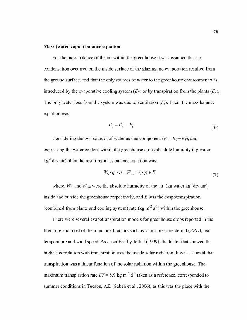
78
Mass (water vapor) balance equation
For the mass balance of the air within the greenhouse it was assumed that no
condensation occurred on the inside surface of the glazing, no evaporation resulted from
the ground surface, and that the only sources of water to the greenhouse environment was
introduced by the evaporative cooling system (EC) or by transpiration from the plants (ET).
The only water loss from the system was due to ventilation (Ev). Then, the mass balance
equation was:
VTC EEE =+ (6)
Considering the two sources of water as one component (E = EC +ET), and
expressing the water content within the greenhouse air as absolute humidity (kg water
kg-1 dry air), then the resulting mass balance equation was:
EqWqW voutvin +⋅⋅=⋅⋅ ρρ (7)
where, Win and Wout were the absolute humidity of the air (kg water kg-1dry air),
inside and outside the greenhouse respectively, and E was the evapotranspiration
(combined from plants and cooling system) rate (kg m-2 s-1) within the greenhouse.
There were several evapotranspiration models for greenhouse crops reported in the
literature and most of them included factors such as vapor pressure deficit (VPD), leaf
temperature and wind speed. As described by Jolliet (1999), the factor that showed the
highest correlation with transpiration was the inside solar radiation. It was assumed that
transpiration was a linear function of the solar radiation within the greenhouse. The
maximum transpiration rate ET = 8.9 kg m-2 d-1 taken as a reference, corresponded to
summer conditions in Tucson, AZ. (Sabeh et al., 2006), as this was the place with the
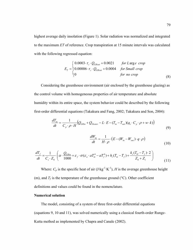
79
highest average daily insolation (Figure 1). Solar radiation was normalized and integrated
to the maximum ET of reference. Crop transpiration at 15 minute intervals was calculated
with the following regressed equation:
⎪⎩
⎪⎨
⎧+⋅⋅+⋅⋅
=cropnofor
cropSmallforQcropeLforQ
E GRoutc
GRoutc
T
00004.000006.0
arg0021.00003.0ττ
(8)
Considering the greenhouse environment (air enclosed by the greenhouse glazing) as
the control volume with homogeneous properties of air temperature and absolute
humidity within its entire space, the system behavior could be described by the following
first-order differential equations (Takakura and Fang, 2002; Takakura and Son, 2004):
( )))((1 kwCqTTELQQ
HCdtdT
pvoutinHeaterGRinp
in ⋅+⋅⋅−−⋅−+⋅⋅
= ρρ (9)
( )ρρ
⋅⋅−−⋅⋅
= qWWEHdt
dWoutin
in )(1
(10)
⎟⎟⎠
⎞⎜⎜⎝
⎛+
⋅−+−+−⋅⋅+⋅⋅
⋅=
10
44
0
2)()()(
10001
ZZTTk
TThaTaTQZCdt
dT fblsfinsfinaf
GRin
s
f εσεα (11)
Where: Cp is the specific heat of air (J·kg-1·K-1), H is the average greenhouse height
(m), and Tf is the temperature of the greenhouse ground (°C). Other coefficient
definitions and values could be found in the nomenclature.
Numerical solution
The model, consisting of a system of three first-order differential equations
(equations 9, 10 and 11), was solved numerically using a classical fourth-order Runge-
Kutta method as implemented by Chapra and Canale (2002).
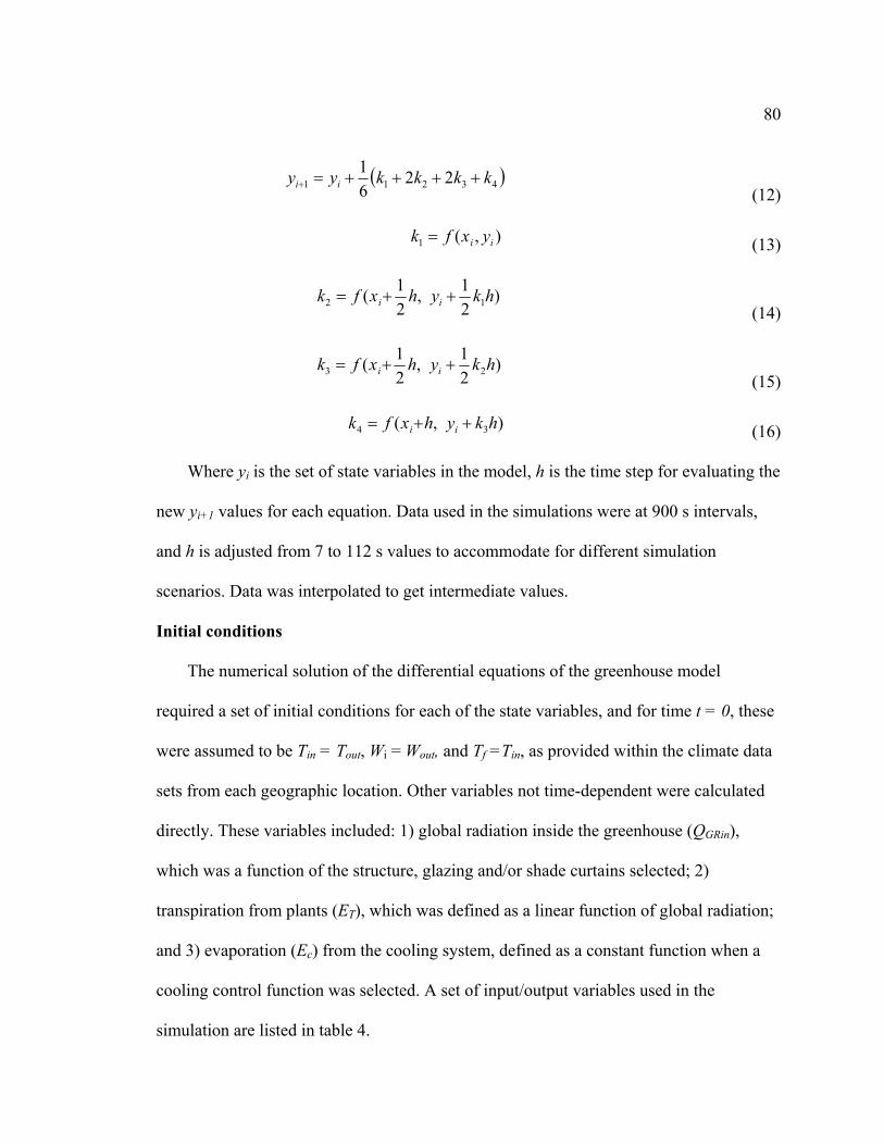
80
( )43211 2261 kkkkyy ii ++++=+
(12)
),(1 ii yxfk = (13)
)21,
21( 12 hkyhxfk ii ++=
(14)
)21,
21( 23 hkyhxfk ii ++=
(15)
),( 34 hkyhxfk ii ++= (16)
Where yi is the set of state variables in the model, h is the time step for evaluating the
new yi+1 values for each equation. Data used in the simulations were at 900 s intervals,
and h is adjusted from 7 to 112 s values to accommodate for different simulation
scenarios. Data was interpolated to get intermediate values.
Initial conditions
The numerical solution of the differential equations of the greenhouse model
required a set of initial conditions for each of the state variables, and for time t = 0, these
were assumed to be Tin = Tout, Wi = Wout, and Tf =Tin, as provided within the climate data
sets from each geographic location. Other variables not time-dependent were calculated
directly. These variables included: 1) global radiation inside the greenhouse (QGRin),
which was a function of the structure, glazing and/or shade curtains selected; 2)
transpiration from plants (ET), which was defined as a linear function of global radiation;
and 3) evaporation (Ec) from the cooling system, defined as a constant function when a
cooling control function was selected. A set of input/output variables used in the
simulation are listed in table 4.

81
Control functions
The resulting greenhouse environment for a specific scenario not only depended on
the external factors (climate), and the response of the inside conditions, but also on the
control schemes implemented on the components of the greenhouse. Control schemes
included reducing the greenhouse air temperature by using shade curtains, by ventilation
or by evaporative cooling, or increasing the air temperature with heaters or by reducing
the ventilation rate.
The simulation of the greenhouse environment was implemented for two general
scenarios: 1) uncontrolled, where initial greenhouse configurations were selected and the
control function of the actuators (shade curtains, ventilation, cooling system, and heaters)
were inactivated; and 2) controlled, where set-points for air temperature (TspD = 24 and
TspN = 18 °C for day and night, respectively) were implemented and the control function
for each component was defined with simple if-then rules to define the status (ON or
OFF) for each component. The values for each of the control components for the ON and
OFF conditions are listed on table 5. For the ON condition, there were 3 levels of Shade,
5 levels of Ventilation, 2 levels of Cooling, 2 levels of Plant sizes, and 2 levels of Heating.
All OFF conditions were zero, except for Ventilation which was 2 hr-1 which represented
a minimum infiltration rate.
The control logic for the shade curtains is defined as: if QGRout > QGRsp then shades
ON, else OFF, where QGRsp, was the threshold value for outside solar radiation, and was
equal to 800 Wm-2.

82
The greenhouse air temperature was controlled by ventilation, evaporative cooling or
by heating, depending if the inside air temperature was greater or less than the air
temperature set-point. In each case there were two conditions, if air temperature was
higher (Tin > Tsp) or lower (Tin < Tsp) than the set-points. In each situation the
corresponding logic values was assigned to activate or de-activate the ventilation, the
evaporative cooling or the heating systems accordingly.
RESULTS AND DISCUSSION
The greenhouse environment model was implemented in an interactive online Web-
based application (http://www.uv.edu/wge/), which incorporated user-selected
information from a database of greenhouse designs, operations, and geographic climate
conditions, and which graphically displayed dynamic changes in the greenhouse
environment. This computer simulation program allowed user/learners to simulate
changes in the plant-greenhouse environment based on climate, structure, and
environmental control choices (Figure 4).
The numerical solution provided a dynamic response of the greenhouse climate to
the outside climate conditions and for a particular greenhouse design. The design
incorporated user-selected inputs for climate, structure, glazing, and environmental
control systems. Each simulation demonstrated the response of a greenhouse system
design over a 28-hour period.
For the given amount of user-selected choices provided by the greenhouse
environment simulator, there are 311,040 possible scenarios which can be demonstrated.
83
The following greenhouse environment simulations were analyzed to show the
potential of the simulator as an educational tool for demonstrating the physics of
greenhouse systems and environmental control principles.
Although the results of the simulated scenarios were not validated with experimental
measurements, they were verified with the logical responses obtained with the control
strategies and the system implemented. As an educational tool the simulator allows for
many scenarios that could be compared side-by-side enhancing the learning experience.
Greenhouse environment simulation with ventilation
In Figure 5 the results of several simulated ventilation and cooling scenarios are
displayed, showing the effect of reduced air movement within a greenhouse. The
environment of an empty greenhouse (A-frame covered with glass) was simulated for the
summer conditions at each of the four locations, and for different ventilation rates (for N
= 2, 10, 20, 30, 60 and 120). The largest air temperature condition occurred when there
was no air exchange (N=2, air exchange due only to infiltration). Greenhouse air
temperatures reached maximum of between 35 and 40 °C in Columbus, OH, between 40
and 45 °C in Burlington, VT, and equal to or higher than 50 °C in Tucson, AZ and Fort
Pierce, FL. By increasing the ventilation rate capacity, the greenhouse air temperature
was reduced to nearly the outside conditions, which was still unfavorable (> 35 °C) for
growing plants. Therefore an artificial cooling mechanism was needed during the summer
season, to maintain the desired greenhouse air temperature (18 and 24 °C for day and
night time, respectively).
84
Greenhouse environment simulation with evaporative cooling
In the previous simulations it was demonstrated that artificial cooling, such as
evaporative cooling system, was required to decrease the greenhouse air temperature. The
cooling effect of the plant canopy on the greenhouse environment was not sufficient in
extremely hot environments, as it will be demonstrated in the following simulation
scenarios. The sensible energy removed by plant transpiration, or evaporated from the
cooling system (evaporative cooling pads, or fogging systems) into latent energy within
the greenhouse environment is affected at different ventilation rates. The cooling
efficiency decreases at higher ventilation rates. Forty-two scenarios were simulated for an
A-frame greenhouse structure covered with glass for spring season conditions in Tucson,
AZ. In Figure 6 each of the lines represents a simulation scenario (with plants size, P=0, s,
or L; and evaporative cooling efficiency, E=0, 1, or 2) at different ventilation rates
(corresponding to N = 2, 10, 20, 30, 60 and 120 h-1). The simulations scenarios include:
1) the cooling effect added by small (PsE0) and large (PLE0) plants with no cooling
system, 2) the effect of the cooling system itself with no transpiration from plants,
working at 50% (P0E1) and at 100% (P0E2) of its capacity, and 3) the combined effect of
transpiration from large plants and the evaporation from cooling systems (PLE1 and
PLE2). The reference values for crop transpiration (ET = 8.9 L m-2 d-1) and evaporation
from cooling system (EC = 14.8 L m-2 d-1) for summer conditions in Tucson, AZ was
determined by Sabeh et al. (2006).
A data point, with the highest air temperature differential (ΔT = Ti - Tout) in a
greenhouse with no ventilation and no evapotranspiration, was taken as a reference in all
85
simulations. This data point was used as a comparison of the air temperature differential
drop when combining the cooling effect of plant transpiration, evaporation from cooling
system and different ventilation rates. The reference point was taken at 13:15 when
outside conditions (Tout = 33.7 °C, RHout = 7.4 %, and QGRout = 1025 W m-2) provided the
greatest cooling needs of the day. To reach the air temperature set-point (24 °C) it was
required to have a ΔT = -9.7 °C which was only reached at simulated low ventilation
rates (N=2 and 10), with maximum cooling efficiency and a large crop (PLE2). The
simulated scenario with a large crop and a deficient cooling system (PLE1) at most will
reach outside conditions, which is not suitable for growing crops. The simulated
scenarios with no evaporative cooling and different crop sizes (PnE0, PsE1 and PnE2)
produced a greenhouse environment more extreme than the outside climate conditions.
Greenhouse environment simulation with shade curtains
The previous simulations scenarios were useful to show that even with a cooling
system the desired greenhouse environment conditions may not be reached, especially
during the hottest part of the day. A well established practice in the greenhouse industry
is the use of internal shade curtains or exterior paints to reduce the heat load during
periods of excessive solar radiation. Shade curtains have the advantage of being
controllable and deployed only when necessary. The following scenarios, which include
the use of shade curtains, were simulated in an Arch-roof greenhouse design covered with
a single layer of polyethylene film for summer conditions in Burlington, VT. The state
variables (QGRin, Tin, Tf, RHin, Win, and VPDin) resulting from the simulated scenarios are
shown in Figure 7. The simulation scenarios included the following combinations: S1

86
(SH=0, P=0, E=0 and N=2), S2 (SH=30, P=L, E=1, and N=30), S3(SH=50, P=L, E=1,
and N=20), and S4 (SH=70, P=L, E=2 and N=20); where SH refers to the % of shade
produced by the shade clothes selected, P refers to the plant size within the greenhouse (0
implies no plants, L is a large crop), E represents the evaporative cooling system capacity
(0 = no cooling system, 1=50 % and 2 = 100% of cooling capacity), and N represents the
ventilation rates expressed as air exchanges per hour. The effect of the shade curtains is
visible on the solar radiation inside the greenhouse for the period of time when the
curtains are deployed. During the daylight time the best greenhouse air temperature
conditions were provided with the scenarios S3 and S4 for the time period of deployed
shade curtains (QGRout > 800 W m-2), after that S4 provided the best conditions (close to
set-points) given the higher capacity of the cooling system. However, at night time S4
resulted in a sub-optimal plant environment with a saturated water vapor environment
due to the cooling system, which followed air temperature set-point.
Greenhouse environment simulation with heating
As shown in Figure 1, three (VT, OH and AZ) of the four locations selected for
simulations require supplementation of heat for some part of the year to maintain the
chosen set-point. This occurs when the average daily air temperature becomes less than
12 °C. The simulation scenarios using a heating system were implemented in an A-frame
structure covered with a single layer tempered glass for winter conditions in Columbus,
OH. Figure 8 include outside climate conditions and the results for each of the
greenhouse state variables at four different scenarios for three heating capacities, during a
28-hour interval. Simulation scenarios include S1 (P=0, N=2 and H0), S2 (P=L, N=2 and
87
H0), S3 (P=L, N=2 and H1), and S4 (P=L, N=2 and H2). Where, H refers to the number
of heating units selected (a single unit heater capacity was predefined as 75 kW). Under
this extreme low temperatures crop production at this season may not be economically
feasible. Scenario S1 shows the increased air temperature during daytime resulting by
solar heat load and the reduced ventilation rate (N2). However, air temperatures were
below freezing (-4 °C) during daytime and even lower during nighttime. Simulation
scenario S2 implemented the same climate control mechanisms (N2 and H0), but now
plants are included. Due to transpiration air temperature dropped 2 °C below the air
temperature of the previous scenario, but now the greenhouse air reached saturation (RH
= 100%) during daytime when plants transpired more water due to solar radiation.
Although air temperature is below freezing it was assumed plants were still alive and
transpiring. Simulation scenario S3 included a heater (H1 = 75 kW) and the simulated
greenhouse air temperature is above 0 °C, it did not reached the daytime and nighttime
set-points. Due to the increased air temperature the air was saturated only a small portion
of the daytime. Simulation scenario S4 included two heaters (H2 = 2 x 75 = 150 kW) and
the simulated greenhouse air temperature were close to the set-points. The increased
water holding capacity of the greenhouse air at the simulated air temperatures resulted in
no saturation and RH was less than 50%.
Limitations of the model
The numerical solution of the system of equations of the model depended on the
initial condition imposed. In all cases the initial conditions were selected equal to the
outside conditions. This was reflected on the lag response at the beginning of the
88
simulation on each of the state variables. Several time steps (h) values in the numerical
implementation were predefined, however they do not perform well in all possible
scenarios.
Input data to the simulator were established at 15 minute intervals. However, for
control purposes this was not an appropriate choice since the actuators response and
operation required time intervals of few second. This resulted in overshooting and
undershooting on the state responses. Also, the control functions for ventilation and
cooling were not staged and they operated at the maximum capacity on the ON position
and to the minimum capacity in the OFF position.
CONCLUSION
The greenhouse environment simulator is a computer simulation program designed
to be used as an education tool for demonstrating the physics of greenhouse systems and
environmental control principles. Given the amount of choices available through the
animated user interface of the simulator, a staggering number (311,040) of possible
scenarios can be replicated, which makes it helpful as an educational tool for
demonstration purposes. We used the simulator to demonstrate how a greenhouse design
could function for several climate conditions (given by the four seasons of four different
locations), and the simulator also indicated what systems may be needed to achieve the
desired environment conditions.
89
The simplified greenhouse environment model produced good approximations of the
dynamic behavior of greenhouse environments with different configurations for 28-hour
simulation periods. The model also was incorporated into a Web-based application where
the simulation scenarios could be replicated without expensive simulation software.
Acknowledgements
This research was funded by a U.S. Department of Agriculture Cooperative State
Research, Education, and Extension Service Higher Education Challenge Grant. We
gratefully acknowledge Marcela Pineros, Andrew Laing, and David Heleba for graphic
design and technical assistance.
REFERENCES
Aaslyng, J.M., J.B. Lund, N. Ehler, and E. Rosenqvist. 2003. IntelliGrow: a greenhouse component-based climate control system. Environmental Modelling & Software. 18: 657-666.
Abdel-Ghany, A.M.and T. Kozai. 2006. Dynamic modeling of the environment in a naturally ventilated, fog-cooled greenhouse. Renewable Energy. 31: 1521-1539.
Al-helal, I.M. 1998. A computational fluid dynamics study of natural ventilation in arid region greenhouses. Ph.D. Thesis, The Ohio State University, Columbus, Ohio.
Arbel, A., M. Barak, and A. Shklyar. 2003. Combination of forced ventilation and fogging systems for cooling greenhouses. Biosystems Engineering. 84: 45-55.
ASAE. 2003. Heating, ventilating and cooling greenhouses. ANSI/ASAE standard EP406.4: 741-749.
Baille, M., A. Baille, and J.C. Laury. 1994. A simplified model for predicting evapotranspiration rate of nine ornamental species vs. climate factors and leaf area. Scientia Horticulturae. 59: 217-232.
90
Bartzanas, T., M. Tchamitchian, and C. Kittas. 2005. Influence of the heating method on greenhouse microclimate and energy consumption. Biosystems Engineering. 91: 487-499.
Blasco, X., M. Martinez, J.M. Herrero, C. Ramos, and J. Sanchis. 2007. Model-based predictive control of greenhouse climate for reducing energy and water consumption. Computers and Electronics in Agriculture. 55: 49-70.
Boulard, T.and A. Baille. 1993. A simple greenhouse climate control model incorporating effects of ventilation and evaporative cooling. Agricultural and Forest Meteorology. 65: 145-157.
Boulard, T.and B. Draoui. 1995. Natural ventilation of a greenhouse with continuous roof vents: measurements and data analysis. Journal of Agricultural Engineering Research. 61: 27-36.
Boulard, T., R. Haxaire, M.A. Lamrani, J.C. Roy, and A. Jaffrin. 1999. Characterization and modelling of the air fluxes induced by natural ventilation in a greenhouse. Journal of Agricultural Engineering Research. 74: 135-144.
Boulard, T.and S. Wang. 2000. Greenhouse crop transpiration simulation from external climate conditions. Agricultural and Forest Meteorology. 100: 25-34.
Chapra, S.C.and R.P. Canale. 2002. Numerical Methods for Engineers: with software and programming applications. McGraw-Hill.
Daskalov, P.I., K.G. Arvanitis, G.D. Pasgianos, and N.A. Sigrimis. 2006. Non-linear adaptive temperature and humidity control in animal buildings. Biosystems Engineering. 93: 1-24.
Dayan, J., E. Dayan, Y. Strassberg, and E. Presnov. 2004. Simulation and control of ventilation rates in greenhouses. Mathematics and Computers in Simulation
Selected papers of the IMACS/IFAC Fourth International Symposium on Mathematical Modelling and Simulation in Agricultural and Bio-Industries. 65: 3-17.
El-Ghoumari, M.Y. 2003. Optimización de la producción de un invernadero mediante control predictivo no lineal. PhD, Universidad Autónoma de Barcelona, Barcelona.
Enoch, H.Z.and Y. Enoch. 1999. The history and geography of the greenhouse, p. 1-15. In: G. Stanhill and H. Zvi Enoch (eds.). Greenhouse ecosystems 20. Elsevier.
Fitz-Rodriguez, E. 2006. Greenhouse environment simulator 1.0: User's manual Vol. 2008.
91
Fitz-Rodriguez, E., C. Kubota, C. Pagliarulo, and G. Giacomelli. 2003. Asynchronous education in controlled environment agriculture. World Conference on E-Learning in Corporate, Government, Healthcare, and Higher Education 2003, Phoenix, Arizona, USA. p. 72-75.
Guzmán, J.L., M. Berenguel, F. RodrÍguez, and S. Dormido. 2005a. Web-based remote control laboratory using a greenhouse scale model. Computer Applications in Engineering Education. 13: 111-124.
Guzmán, J.L., F. Rodríguez, M. Berenguel, and S. Dormido. 2005b. Virtual lab for teaching greenhouse climate control. 16th IFAC World Congress, Prague, Czech Republic.
Hanan, J.J. 1998. Greenhouses : advanced technology for protected horticulture. CRC Press, Boca Raton, Fla. ; London.
Jolliet, O. 1994. HORTITRANS, a model for predicting and optimizing humidity and transpiration in greenhouses. J. agric. Engng. Res. 57: 23-37.
Jolliet, O. 1999. Water cycle, p. 303-326. In: G. Stanhill and H. Zvi Enoch (eds.). Greenhouse ecosystems 20. Elsevier.
Jones, J.W., E. Dayan, P. Jones, Y. Hwang, and B.K. Jacobson. 1988. Modeling tomato growth for greenhouse environment control. International winter meeting of the ASAE, Chicago, IL.
Jones, J.W., E. Dayan, H. van Keulen, and H. Challa. 1989. Modeling tomato growth for optimizating greenhouse temperatures and carbon dioxide concentrations. Acta Hort. (ISHS). 248: 285-294.
Jones, P., J.W. Jones, and Y. Hwang. 1990. Simulation for determining greenhouse temperature setpoints. Transactions of the ASAE. 33: 1722-1728.
Jong, T.d. 1990. Natural ventilation of large multi-span greenhouses. Ph.D., Wageningen Agricultural University, Wageningen.
Kempkes, F.L.K., N.J. Van de Braak, and J.C. Bakker. 2000. Effect of heating system position on vertical distribution of crop temperature and transpiration in greenhouse tomatoes. Journal of Agricultural Engineering Research. 75: 57-64.
Körner, O. 2003. Crop based climate regimes for energy saving in greenhouse cultivation. Ph.D., Wageningen Agricultural University, Wageningen.
Korner, O.and H. Challa. 2003. Process-based humidity control regime for greenhouse crops. Computers and Electronics in Agriculture. 39: 173-192.

92
Linker, R., I. Seginer, and P.O. Gutman. 1998. Optimal CO2 control in a greenhouse modeled with neural networks. Computers and Electronics in Agriculture. 19: 289-310.
Ramirez-Arias, A. 2005. Control jerárquico multiobjetivo de crecimiento de cultivos bajo invernadero. PhD, Universidad de Almería.
Sabeh, N.C., G.A. Giacomelli, and C. Kubota. 2006. Water use for pad and fan evaporative cooling of a greenhouse in a semi-arid climate. Acta Hort. (ISHS). 719: 409-416.
Seginer, I. 1993. Crop models in greenhouse climate control. Acta Horticulturae. 328: 79-98.
Seginer, I., A. Angel, and D. Kantz. 1986. Optimal CO2 enrichment strategy for greenhouses: a simulation study. Journal of Agricultural Engineering Research. 34: 285-304.
Stanghellini, C.and W.T.m. van Meurs. 1992. Environmental control of greenhouse crop transpiration. Journal of Agricultural Engineering Research. 51: 297-311.
Stanhill, G.and H. Zvi Enoch. 1999. Greenhouse Ecosystems. In: D.W. Goodall (Ed., Ecosystems of the World 20 Vol. 20, Elsevier, pp. 423.
Takakura, T. 1976. Development of VETH chart using computer, p. 96-97. Technical report on design standards of greenhouse environmental control systems. University of Tokyo.
Takakura, T.and W. Fang. 2002. Climate under cover. Kluwer Academic Publishers.
Takakura, T., K.A. Jordan, and L.L. Boyd. 1971. Dynamic simulation of plant growth and environment in the greenhouse. Transactions of the ASAE. 14: 964-971.
Takakura, T.and J.E. Son. 2004. Simulation of biological and environmental processes. Kyushu University Press.
Tap, F. 2000. Economics-based optimal control of greenhouse tomato crop production. Ph.D., Wageningen Agricultural University, Wageningen.
Tignor, M.E., G.A. Giacomelli, S.B. Wilson, C. Kubota, E. Fitz-Rodriguez, T.A. Irani, E.B. Rhoades, and M.J. McMahon. 2006. Development of a web-based multi-media resource for environmental control modeling and greenhouse education. Acta Horticulturae. 719: 303-310.
Tignor, M.E., S.B. Wilson, G.A. Giacomelli, C. Kubota, E. Fitz-Rodriguez, T.A. Irani, E.B. Rhoades, and M.J. McMahon. 2007. Multi-institutional cooperation to
93
develop digital media for interactive greenhouse education. Hort. Technology. 17: 297-399.
Tignor, M.E., S.B. Wilson, L. Hightower, E. Fitz, G.A. Giacomelli, C. Kubota, E.B. Rhoades, T.A. Irani, M.J. McMahon, A. Laing, D. Heleba, and S. Greenleaf. 2005. Integrating video, interactive animations, images, and assessment towards an expandable instructor resource. HortScience. 40: 1044.
Udink ten Cate, A.J. 1983. Modeling and (adaptive) control of greenhouse climates. Ph.D., Wageningen Agricultural University, Wageningen.
van Henten, E.J. 1994. Greenhouse climate management: An optimal control approach. Ph.D., Wageningen Agricultural University, Wageningen.
van Straten, G., H. Challa, and F. Buwalda. 2000. Towards user accepted optimal control of greenhouse climate. Computers and Electronics in Agriculture. 26: 221-238.
von Zabeltitz, C. 1999. Greenhouse structures, p. 17-69. In: H. Zvi Enoch (ed.). Greenhouse ecosystems 20. Elsevier.
Willits, D.H. 2003. Cooling Fan-ventilated Greenhouses: a Modelling Study. Biosystems Engineering. 84: 315-329.
Zwart, H.F.d. 1996. Analyzing energy-saving options in greenhouse cultivation using simulation model. Ph.D., Wageningen Agricultural University, Wageningen.
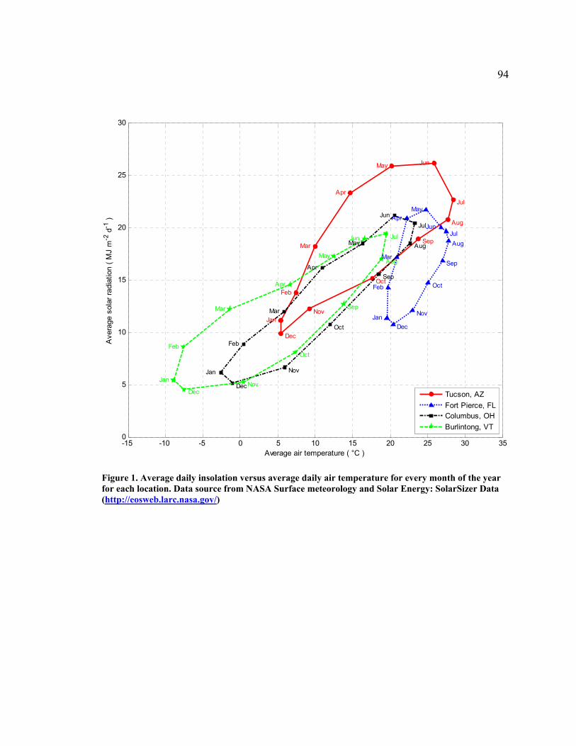
94
-15 -10 -5 0 5 10 15 20 25 30 350
5
10
15
20
25
30
Jan
Feb
Mar
Apr
May Jun
Jul
Aug
gSep
SeOct
Nov
Dec
Jan
JanJan
Feb
FebFeb
Mar
MarMar
Apr
Apr
Apr
May
May
May
Jun
Jun
Jun Jul
Jul
JulAugAu
Aug Sep
p
Sep
Oct
Oct
Oct
Nov
Nov
Nov
Dec
DecDec
Average air temperature ( °C )
Ave
rage
sol
ar ra
diat
ion
( MJ
m -2 d
-1 )
Tucson, AZFort Pierce, FLColumbus, OHBurlintong, VT
Figure 1. Average daily insolation versus average daily air temperature for every month of the year for each location. Data source from NASA Surface meteorology and Solar Energy: SolarSizer Data (http://eosweb.larc.nasa.gov/)

95
Figure 2. Structural designs implemented in the greenhouse environment simulator. All three designs have 30 m of length, and are single-span. Units are in meters.
α
ρ
τ
QGRout
QIV
QHeater
QGlazing
{Tin, RHin, Win}
QGround
{Tout, RHout, Wout}
EC
ETQGRin
EV ET
Figure 3. Energy and water vapor fluxes within the greenhouse which define the energy and mass balance equations. See Table of Nomenclature for definitions of each parameter and variable.

96
Figure 4. Screen capture of the simulator after running a simulation of the greenhouse environment for winter conditions in Tucson, AZ.
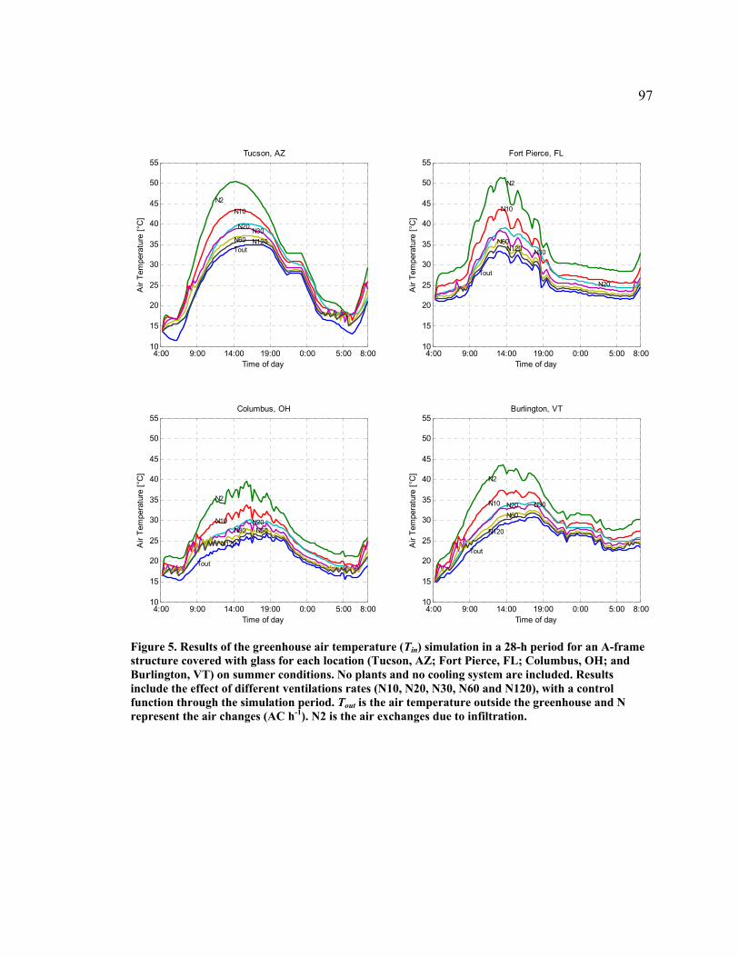
97
4:00 9:00 14:00 19:00 0:00 5:00 8:0010
15
20
25
30
35
40
45
50
55Tucson, AZ
Air
Tem
pera
ture
[°C
]
Tout
N2N10
N20 N30N60 N120
Time of day4:00 9:00 14:00 19:00 0:00 5:00 8:00
10
15
20
25
30
35
40
45
50
55Fort Pierce, FL
Air
Tem
pera
ture
[°C
]
Tout
N2
N10
N20
N30N60
N120
Time of day
4:00 9:00 14:00 19:00 0:00 5:00 8:0010
15
20
25
30
35
40
45
50
55Columbus, OH
Air
Tem
pera
ture
[°C
]
Tout
N2
N10 N20N30 N60
N120
Time of day4:00 9:00 14:00 19:00 0:00 5:00 8:00
10
15
20
25
30
35
40
45
50
55Burlington, VT
Air
Tem
pera
ture
[°C
]
Tout
N2
N10 N20 N30N60
N120
Time of day
Figure 5. Results of the greenhouse air temperature (Tin) simulation in a 28-h period for an A-frame structure covered with glass for each location (Tucson, AZ; Fort Pierce, FL; Columbus, OH; and Burlington, VT) on summer conditions. No plants and no cooling system are included. Results include the effect of different ventilations rates (N10, N20, N30, N60 and N120), with a control function through the simulation period. Tout is the air temperature outside the greenhouse and N represent the air changes (AC h-1). N2 is the air exchanges due to infiltration.

98
-15
-10
-5
0
5
10
15
20
0.003 0.014 0.029 0.043 0.086 0.172
Ventilation rate qv ( m3 m-2 s-1 )
(Tin
- T o
ut) (
°C) PnE0
PsE0PLE0PnE1PLE1PnE2PLE2
Figure 6. Simulation results of an A-frame structure covered with glass and located in Tucson, AZ. Data points represent the air temperature differential (Tin –Tout) during the hottest part of the day for spring conditions at different ventilation rates and different scenarios. Outside climate conditions are Tout = 33.7 °C, RHout = 7.4 %, and QGRout = 1025 W m-2. Simulation scenarios include no plants (Pn), small plants (Ps), large plants (PL), in combination with three evaporative cooling capacities, at 0, 50 and 100% (E0, E1, and E2 respectively).
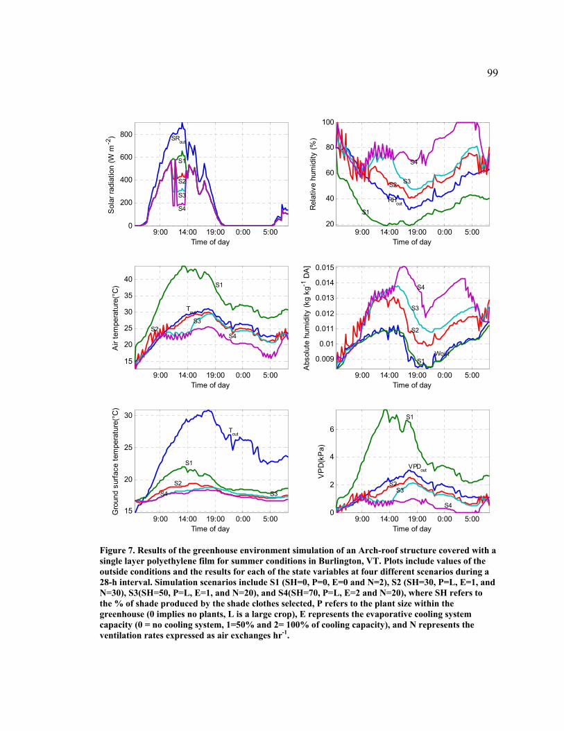
99
9:00 14:00 19:00 0:00 5:000
200
400
600
800
Sol
ar ra
diat
ion
(W m
-2) SRout
S1
S2
S3
S4
Time of day9:00 14:00 19:00 0:00 5:00
20
40
60
80
100
Rel
ativ
e hu
mid
ity (%
)
RHout
S1
S2 S3
S4
Time of day
9:00 14:00 19:00 0:00 5:00
15
20
25
30
35
40
Air
tem
pera
ture
(°C
)
Tout
S1
S2S3
S4
Time of day9:00 14:00 19:00 0:00 5:00
0.009
0.01
0.011
0.012
0.013
0.014
0.015
Abs
olut
e hu
mid
ity (k
g kg
-1 D
A]
WoutS1
S2
S3
S4
Time of day
9:00 14:00 19:00 0:00 5:0015
20
25
30
Gro
und
surfa
ce te
mpe
ratu
re(°
C)
Tout
S1
S2S3S4
Time of day9:00 14:00 19:00 0:00 5:00
0
2
4
6
VP
D(k
Pa)
VPDout
S1
S2S3
S4
Time of day
Figure 7. Results of the greenhouse environment simulation of an Arch-roof structure covered with a single layer polyethylene film for summer conditions in Burlington, VT. Plots include values of the outside conditions and the results for each of the state variables at four different scenarios during a 28-h interval. Simulation scenarios include S1 (SH=0, P=0, E=0 and N=2), S2 (SH=30, P=L, E=1, and N=30), S3(SH=50, P=L, E=1, and N=20), and S4(SH=70, P=L, E=2 and N=20), where SH refers to the % of shade produced by the shade clothes selected, P refers to the plant size within the greenhouse (0 implies no plants, L is a large crop), E represents the evaporative cooling system capacity (0 = no cooling system, 1=50% and 2= 100% of cooling capacity), and N represents the ventilation rates expressed as air exchanges hr-1.
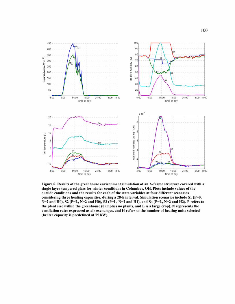
100
4:00 9:00 14:00 19:00 24:00 5:00 8:00
50
100
150
200
250
300
350
400
450S
olar
radi
atio
n (W
m-2
)SRout
SRin
Time of day4:00 9:00 14:00 19:00 24:00 5:00 8:00
20
30
40
50
60
70
80
90
100
Rel
ativ
e hu
mid
ity (%
) RHout
S1
S2
S3
S4
Time of day
4:00 9:00 14:00 19:00 24:00 5:00 8:00
-10
-5
0
5
10
15
20
Air
tem
pera
ture
(°C
)
Tout
S1
S2
S3
S4
Time of day4:00 9:00 14:00 19:00 24:00 5:00 8:001
2
3
4
5
6
x 10-3
Abs
olut
e hu
mid
ity (k
g kg
-1 D
A]
Wout S1
S2
S3
S4
Time of day Figure 8. Results of the greenhouse environment simulation of an A-frame structure covered with a single layer tempered glass for winter conditions in Columbus, OH. Plots include values of the outside conditions and the results for each of the state variables at four different scenarios considering three heating capacities, during a 28-h interval. Simulation scenarios include S1 (P=0, N=2 and H0), S2 (P=L, N=2 and H0), S3 (P=L, N=2 and H1), and S4 (P=L, N=2 and H2). P refers to the plant size within the greenhouse (0 implies no plants, and L is a large crop), N represents the ventilation rates expressed as air exchanges, and H refers to the number of heating units selected (heater capacity is predefined at 75 kW).

101
Table 1. Dimensions and properties of greenhouse designs used in the simulations Property A-frame Arch-Roof Quonset Length (m) 30 30 30 Width (m) 10 10 8 Gutter high (m) 4 4 - Ridge high (m) 6.3 6.3 4 Afl (m2) 300 300 240 Agl (m2) 713 692 427 Volume (m3) 1545 1680 745 w ratio (Agl/Afl) 2.5 2.3 1.8
Table 2. Properties of the greenhouse glazing materials used in the simulations
Layers
Greenhouse glazing
k-value A (W·m-2·°C-1)
Light Transmissivity B (%)
Glass 6.2 90
Polyethylene 6.2 87
Single
Polycarbonate 6.2 87
Polyethylene 4.0 76 Double
Polycarbonate 3.3 79
A Taken from ANSI/ASAE EP406.3 B Taken from Hanan (1998) Table 3. Ventilation rates (m3 m-2 s-1) implemented with the simulation for each greenhouse structural design. Air exchanges per hour (h-1)
Ventilation rate (m3 m-2 s-1)
N A-frame Arch-Roof Quonset 2 0.003 0.003 0.002
10 0.014 0.016 0.009 20 0.029 0.031 0.018 30 0.043 0.047 0.026 60 0.086 0.093 0.052 120 0.172 0.187 0.105

102
Table 4. Input and output parameters in the greenhouse environment model. Primary
Variables Units
Derived Variables
Units
Time s QGRout Wm-2 Wout kgwater kg-1
dry air Tout °C Wsout kgwater kg-1
dry air Input
RHout % VPDout kPa QGRin Wm-2 Tin °C Wsin kgwater kg-1
dry air Win kgwater kg-1
dry air RHin % Output
Tf °C VPDin kPa
Table 5. Values for the ON-OFF condition for each of the control components for modifying the greenhouse environment. Status Component Predefined value ON OFF Shade curtains Percent of Shades (%) 30
50 70
0
Ventilation rate (Natural or Forced)
Air exchanges N = (h-1) 10 20 30 60 120
2
Cooling system Ec = 14.8 (kg m-2d-1) A 0.5 1.0
0
Heating System NH (Hcap = 75 kW) 1 2
0
A Values taken from (Sabeh et al., 2006)
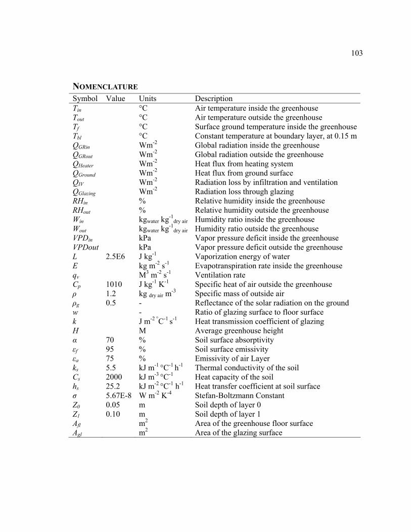
103
NOMENCLATURE Symbol Value Units Description Tin °C Air temperature inside the greenhouse Tout °C Air temperature outside the greenhouse Tf °C Surface ground temperature inside the greenhouseTbl °C Constant temperature at boundary layer, at 0.15 m QGRin Wm-2 Global radiation inside the greenhouse QGRout Wm-2 Global radiation outside the greenhouse QHeater Wm-2 Heat flux from heating system QGround Wm-2 Heat flux from ground surface QIV Wm-2 Radiation loss by infiltration and ventilation QGlazing Wm-2 Radiation loss through glazing RHin % Relative humidity inside the greenhouse RHout % Relative humidity outside the greenhouse Win kgwater kg-1
dry air Humidity ratio inside the greenhouse Wout kgwater kg-1
dry air Humidity ratio outside the greenhouse VPDin kPa Vapor pressure deficit inside the greenhouse VPDout kPa Vapor pressure deficit outside the greenhouse L 2.5E6 J kg-1 Vaporization energy of water E kg m-2 s-1 Evapotranspiration rate inside the greenhouse qv M3 m-2 s-1 Ventilation rate Cp 1010 J kg-1 K-1 Specific heat of air outside the greenhouse ρ 1.2 kg dry air m-3 Specific mass of outside air ρg 0.5 - Reflectance of the solar radiation on the ground w - Ratio of glazing surface to floor surface k J m-2 °C-1 s-1 Heat transmission coefficient of glazing H M Average greenhouse height α 70 % Soil surface absorptivity εf 95 % Soil surface emissivity εa 75 % Emissivity of air Layer ks 5.5 kJ m-1 °C-1 h-1 Thermal conductivity of the soil Cs 2000 kJ m-3 °C-1 Heat capacity of the soil hs 25.2 kJ m-2 °C-1 h-1 Heat transfer coefficient at soil surface σ 5.67E-8 W m-2 K-4 Stefan-Boltzmann Constant Z0 0.05 m Soil depth of layer 0 Z1 0.10 m Soil depth of layer 1 Afl m2 Area of the greenhouse floor surface Agl m2 Area of the glazing surface
104
APPENDIX B: TOMATOES LIVE! 2.0: A WEB-BASED GREENHOUSE MONITORING SYSTEM
E. Fitz-Rodríguez, and G. A. Giacomelli
Department of Agricultural and Biosystems Engineering, University of Arizona Tucson, AZ.
105
ABSTRACT
Greenhouse technologies are used in the production of vegetables, ornamentals,
transplants, and other plant products providing added value. Sophisticated greenhouse
production techniques rely on the use of computer technologies both for monitoring and
for precise control of the processes involved in the production cycle of high quality plant
products. Knowing the status of the plant-greenhouse system in real time, requires the use
of sensors and controllers for monitoring and controlling each of the environmental
variables. Due to need of environmental control responses to the continually changing
outdoor climate, and the potential failure of the systems within the controlled
environment system, it is valuable to have an information system capable of off-site
monitoring of the greenhouse environment. Internet technologies offer a possible means
of communication. A Web-based monitoring system called “Tomatoes Live! 2.0” was
developed to oversee greenhouse production in educational and research facilities. The
monitoring system was implemented in several research units and in a greenhouse
educational laboratory at the Controlled Environment Agriculture Center (CEAC) of The
University of Arizona. “Tomatoes Live! 2.0” is accessible to researchers, students and the
general public through the Web at http://ag.arizona.edu/ceac/live2/, where an array of
web-cameras provides a visual accounting of the current crop conditions at each unit,
while real-time greenhouse environmental data and related plant oriented calculated
parameters are displayed. The system has been successfully used since its implementation
in 2001, and it has proved to be valuable not only as an educational tool, but also as an
instrument for remote diagnostics.

106
Keywords: Greenhouse environment control, remote diagnosis, teleagriculture,
Web-based monitoring, crop monitoring system, Internet, Java, WLAN
107
INTRODUCTION
Crop production within Controlled Environment Agriculture (CEA) has been
successfully utilized for production of vegetables, ornamentals, transplants and many
other plant materials with high economic value. In the future it will be used not only for
such plant products, but in even more valuable applications of plant bio-processing. The
natural plant physiological processes will become the living plant bio-processors and
provide environmental remediation of soil, air and water, phytochemical production of
nutraceuticals, and bio-pharmaceutical production of functional antigens (Chikwamba et
al., 2002; Sijmons et al., 1993; Stevens et al., 2007).
The greenhouse industry in the USA has a total of approximately 12,684 ha, with
almost 600 ha dedicated to the production of vegetables, and 12,085 ha dedicated to the
floriculture crop production (USDA, 2002). Although CEA promises high efficiency in
the use of resources, such as land, water, labor, energy, capital, and increased
productivity and quality compared to traditional field production, CEA is highly
dependent on energy, skilled labor, effective management and increased knowledge of
growing specific crops (Giacomelli et al., 2007; Jensen, 2002). Energy and labor
availability and operations costs remain the most significant concern of a greenhouse
operation. Furthermore the increased consumer demand for environmentally friendly
production, healthy and safe foods, and locally grown products has contributed to the
growth of CEA from 7,934 ha in 1997 to 12,684 ha in 2002 (USDA, 2002). CEA is a
highly capital intensive and a technologically demanding agricultural practice, which has
come to rely more on computer-based technologies for monitoring the plant environment,
108
organizing and evaluating plant response to the environment (yields), and for making
accurate and informed decisions about the crop management within the different time
scales, ranging from hourly, daily, weekly, seasonally, to yearly for controlling each of
the processes in the production cycle.
A crop-greenhouse system is subject to unexpected disturbances, caused by variable
outdoor climate conditions, and the latent ineffective response of the climate control
systems to correct the disturbances and return the environment to nominal conditions.
Description of greenhouse climate controllers
Most commercially available greenhouse climate controllers consist of two
components: 1) the climate controller hardware which allows for automatic monitoring
and control, and includes the main computer controller, sensors and actuators; and 2) a
personal computer (PC) acting as a server that is directly connected (usually by a RS-232
serial port) to the climate controller. The server PC includes software that allows for data
recording and for accessing all the control features of the climate controller where real
time climate data and actuator status can be displayed, and provides for the manipulation
of set-point values on each of the controlled parameters. Access to the server PC could
be established by remote communication either by phone lines or Ethernet ports in a
single or multi-user fashion (depending on the capabilities of the climate controller
software). However most server software has a closed architecture which limits the
capability of implementing third party software or algorithms with models for climate
control with either plant-based or energy-efficiency objectives (Ehler, 1991; Ehret et al.,
2001). Another disadvantage of closed architectures is the obligatory use of the
109
proprietary software, limiting its ability to remotely access the information regarding the
status of the plant-greenhouse system.
Opportunities for improving the monitoring of greenhouse crops
Web-based technologies could extend the capabilities of off-site monitoring without
the need of special software, other than a web browser and a PC with access to the
Internet. This will increase the possibility of remote diagnosis through telepresence
(Giacomelli et al., 2007) when expertise is not locally available, as well as awareness of
the status of the plant-greenhouse system without being bounded in time or space.
In educational and research centers where multidisciplinary collaboration occurs,
having systems capable of off-site monitoring is of great importance because it both
allows researches and faculty to remotely view the ongoing research and oversee
potential problems, and allows access for students and the general public with interest in
the specific project, or CEA in general.
Internet technologies in greenhouse climate controllers
Despite its potential, internet technologies in CEA have been implemented mainly in
research facilities, for example Ehler and Aaslyng (2001) developed a dynamic internet
application which allowed access to real-time climate data and basic control parameters
from a greenhouses complex at the Royal Agricultural University of Copenhagen, DK.
They developed two components: BispArch and CYBGR4 (Aaslyng et al., 2005) which
were software components which enabled the synchronization of data from several
greenhouse climate computers into one computer and also the dynamic generation of

110
climate data into HTML format for automatic upload on a Web server. Further
development led to the creation of IntelliGro, a greenhouse climate control system suited
for decreasing energy consumption while achieving higher or equal plant production
(Aaslyng et al., 2003).
Morais and Cunha (2000) developed a networked system (Agritronics) to monitor
and control a group of university greenhouse facilities located in Portugal. Another web-
based application was developed by Lopes et al. (2002) using Java applets that were
designed to share images of crops within a controlled environment system in the
agricultural automation laboratory of the University of São Paulo, Brazil. This system
proved to be a low-cost and effective tool which enabled sharing images of the
production system over the Internet, and increased the capability of technical support
world wide.
Motivation for further developments
Controlled environment systems are technically advanced intensive agricultural
systems, and a failure of any part of the complex system, for even a short time period,
could lead to a loss of the highly valuable crop. For this reason it is beneficial to have a
monitoring system capable of provide real-time information of the entire system 24 hrs a
day which could be accessed from any computer or any other mobile device (cell phone
or other electronic communication device) with access to the Internet. A system with
these characteristics broadens our capabilities to share crop production expertise and
enhances learning. Also by remotely inspecting the crop, the probability of diagnosis and
problem correction in a timely manner will increase the potential for production success.

111
This system could also be useful in other arenas, for example, in academia where
regular visits to the facilities are not possible, in large production systems where qualified
staff is limited, or in production systems located in hostile environments, such as the
South Pole (Giacomelli et al., 2007).
The objective of the current research was to develop a web-based monitoring system
for plant production in controlled environments that provided historical and real-time
environmental data and real-time images of the plant-greenhouse system, in a reliable and
efficient way that would offer decision-support capabilities through telepresence
activities.
Current status of greenhouse monitoring systems
The development of research and educational facilities and their subsequent
monitoring and control systems is generally an evolutionary process that occurs in stages
over time resulting with various technologies (greenhouse climate controllers and the
software to operate them) in different research units. As a result, retrieving and sharing
data in a standardized way is complicated and cumbersome.
The greenhouse complex and research facilities of the Controlled Environment
Agriculture Center (CEAC), at the College of Agriculture and Life Sciences at The
University of Arizona which are located at and operated by the Campus Agricultural
Center (CAC), included several vendor-specific greenhouse climate control technologies,
including Grower’s Choice Environmental Controller (HortiMax USA Inc., formerly Q-
COM Corp, Rancho Santa Margarita, CA, USA), Argus Controls (Argus Control
Systems Ltd. White Rock, British Columbia, Canada), and Wadsworth climate
112
controllers (Wadsworth Control Systems Inc., Arvada, CO, USA). Also there are several
data acquisition systems tailored for specific research monitoring needs, including
Campbell data loggers (Campbell Scientific, Inc. North Logan, Utah, USA), and HOBO
Temp/RH Data Loggers (Onset Computer Corporation, Bourne, MA, USA). The
Grower’s Choice Environmental Controller and the Argus Controls systems include
proprietary software that do not allow a direct interaction with its software, and/or direct
communication with the hardware component due to a closed architecture or to the lack
of communication drivers to the micro-controllers. However they are capable of
producing a report in ASCII format that could be accessed with third party software and
thus extend their web-based capability. Originally data was only stored locally within the
climate controllers, or in the case of the data-loggers from Campbell Scientific (Models
21X and 23X), data was manually downloaded on a weekly basis by using transportable
data storage modules.
The first version of “Tomatoes live!” was implemented in 2001 (Choi et al., 2002;
Fitz-Rodriguez et al., 2003), where only a greenhouse educational lab was monitored
through the Grower’s Choice Environmental Controller, and provided real-time
environmental data, as well as two web cameras providing a panoramic view and a close
view of a cluster of tomatoes on the vine. The current version (Tomatoes Live! 2.0) has
been enhanced and includes the capabilities of the first version, as well as an extended
monitoring capabilities to several other research facilities and greenhouses operating with
different greenhouse climate controllers or data acquisition systems. In addition, data
processing was added to increase the capability of displaying a wider range of data,
113
including every 7-day period, and plant-oriented environmental parameters within the
graphical interface. Each site was also provided a network camera to permit visual
inspection of the plants and their production systems.
NEW PROPOSED ARCHITECTURE
The proposed architecture for the new Web-based greenhouse monitoring system
consisted of two parts: 1) a hardware component that included the greenhouse climate
controllers, data loggers and devices that integrate and extend the data communication
through the local area network (LAN) or wireless LAN (WLAN); and 2) a software
component, consisting of several scripts, programs and server applications that make the
information available trough the Web in near real-time (updated at 5 minute intervals)
Hardware and Infrastructure
The research greenhouses of the CEAC are located in close proximity to the CEAC
main buildings where LAN and WLAN infrastructure existed. Data communication from
the greenhouses was implemented trough Wired Ethernet LAN (IEEE 802.3) and
Wireless LAN (IEEE 802.11 b/g/n) of the existing infrastructure. Where necessary,
wireless devices were installed to extend the reach of data communication. Several
Access Points and Wireless Bridges were used in remote greenhouses where no Ethernet
infrastructure was available.
Each of the research greenhouses of the CEAC has a greenhouse climate micro-
controller and a PC directly connected through a RS-232 serial port. These computers run
a server program, specific for each greenhouse climate micro-controller, which is able to
114
display and record data from the sensors and actuators, and also to manipulate set-points
of environmental parameters. Each of these computers also has a direct connection
through the LAN or WLAN which enables the communication. Figure 1 includes a
diagram of the existing greenhouse infrastructure and a schematic representation of how
data was transmitted from the greenhouse microcontrollers and research-oriented data-
logger units, to the Web server where the information was readily available.
Data communication
The first layer of data communication occurred between the sensors/actuators and the
micro-controller of each greenhouse, or between the sensors and data-loggers units.
The second layer of data communication occurred between the micro-controller units
and a dedicated PC (personal microcomputer) with special software for each of the
systems. Up to this layer the systems are well established and operated successfully but
independently. Access to each of the dedicated PCs associated with each greenhouse
microcontroller and research-oriented data-logger unit was only possible, either on-site or
remotely, if a licensed remote desktop software (client/server) was available on each
dedicated PC, which is usually run over Internet protocols. This procedure, with remote
desktop is generally not satisfactory because it is too slow as a result of high network
traffic or slow Internet connectivity. Furthermore, most remote desktop applications are
limited to single sessions. The licensed client program although functional, requires
additional cost during the purchase of the monitoring system.
The third layer of communication occurred between the dedicated PC and a PC
acting as a data collector. Each dedicated PC shared a folder over the Microsoft®

115
Network, where new data was updated in text files (ASCII) at five minutes intervals. In
this stage the data collector PC ran several programs to pre-process raw data (implements
SI units, convert date and time from strings to numeric values, compute new parameters,
and check for data errors), and then upgraded new records within the stored files.
The fourth layer of communication was between the data collector PC and the Web
server, where the newly preprocessed and updated data was available and ready to be
transmitted to the Web server.
The fifth layer of communication occurred whenever a user sent a request to the
HTTP server by accessing the Web page of the greenhouse monitoring system
(http://ag.arizona.edu/ceac/live2/) through a client Web browser.
Q-COM Climate micro-controller
Wadsworth Climate controller &
Data Loggers
Argus Climate micro-controller
Computer Running Climate controller Software
(QCOM)
LAN
Computer Running Climate controller Software
(ARGUS)
RS232
RS232 to Wireless
RS232
Computer Running Data Logger Software
(LoggerNet)
Computer running software to gather data from all greenhouses and transfer
it to the Web server
HTTPServer
WLAN
Research Greenhouses
Web Browsers
(Client) (Server)
INTERNET
Layer 1
Layer 2
Layer 3
Layer 4
Layer 5 Data collector PC
Dedicated PCs
Figure1. Diagram of hardware components and data transmission

116
Wireless infrastructure
To extend the capabilities of data and image transmission at each of the research
greenhouses, an Ethernet LAN (IEEE 802.3) and a Wireless LAN (IEEE 802.11 b/g/n)
infrastructure was established. Network devices such as: Switches, Bridges, Wireless
Access Points, Wireless Routers, Wireless Network Cards, and Wireless Serial Servers,
were installed throughout the facilities.
Wireless communication was implemented at distant greenhouses for interfacing
data loggers and wireless networked cameras. For a direct communication to the data
loggers over the LAN or WLAN, two types of devices were implemented: 1) Wireless
802.11b/g Serial Servers models ES1AWB and ESR901W232 (B&B Electronics Mfg.
Co. Inc., Ottawa, IL, USA), which interfaced data loggers (Campbell Scientific 21X and
23x) from a RS-232 serial port directly to the WLAN; and 2) NL100 Network Link
Interface (Campbell Scientific, Inc. North Logan, Utah, USA) that communicate with
Campbell Scientific Data-loggers (21x and 23x) using and Ethernet 10-Base-T
communication link from the CS 1/O or RS-232 ports and directly to the LAN.
In remote greenhouses where Ethernet ports were not available, Wireless Bridges
model WET200 (Linksys, Cisco Systems Inc., Irvine, CA, USA) were installed to extend
the wireless signal range and to have local Ethernet ports available to connect NL100
devices, PCs or Network Cameras.
Visual monitoring
Several visual monitoring devices (web cameras) have been tested and implemented
throughout the development of this project. As the technology evolved, there was an

117
increase in capabilities and a reduction of costs. The two types of network cameras used
enabled communication through Wireless LAN (IEEE 802.11b).
The first type of web camera was the Axis network camera model 207MW (Axis
Communications AB, Lund, Sweden) which was used to have an overall view of the crop,
and for closer examination of a specific part of the plant (for example, to watch and
record a tomato cluster’s growth and development).
The second type of camera was a Sony Pan-Tilt-Zoom (PTZ) network camera model
SNC-RZ30N (Sony Corp., San Diego, CA, USA) which could be remotely controlled
over the internet. This camera allowed users to direct the web camera to specific
locations within the greenhouse, or on the crop, such as the whole plant, leaves, flowers,
stems, heads, etc.
Software component
The software component of the greenhouse monitoring system consisted of several
programs and scripts implemented in two computers: 1) a PC dedicated to pre-processing
and uploading of newly recorded data from all greenhouses and data-loggers, and 2) a
server hosting the user interface and readily available data.
Data collection and pre-processing
The data collector PC implemented and ran several scripts and programs for
retrieving data from the dedicated PCs (running software for each greenhouse climate
controller and for each data-logger) at different time intervals. The climate controller
software on each of the dedicated PCs created a text (ASCII) file which included new

118
records of parameters of interest. These files were placed within folders which were
password protected and shared over the Microsoft® Network. On the data collector PC,
the shared folders of the dedicated PCs were mapped into network drives for quick access.
A set of three batch files, which were scripts running several programs and commands,
were implemented in the data collector PC within the Microsoft® Windows Scheduler as
shown in Figure 2.
Microsoft Windows Scheduler
Script #1 “ClmUpdate” (running at 5-min intervals) • Copy raw data from dedicated PCs. • Run “clmUpdate.exe” program (to clean, transform,
convert units, and format data). • Transfer new created files to the Web Server via FTP
protocol.
Script #2 “ClmSummary” (running at 24-h intervals) • Copy recently formatted data file from script #1 into
a local directory. • Run “clmSummary.exe” program (to create a
summary of daily climate data). • Append daily climate summary to daily record.
Script #3 “ClmBackup” (running at 7-d intervals) • Copy raw data from dedicated PCs. • Run “clmBackup.exe” program (to create back-ups of
data from previous week). • Create data back-ups on the local PC and on the server
for access to historical data (older than seven days).
Figure 2. Scripts and programs running at the data collector PC.
Data from each of the greenhouse climate controllers and data loggers differed in
format, units, and methods by which they were stored. While Q-COM software stored
records on a single file, which included several columns of no usage, Argus software
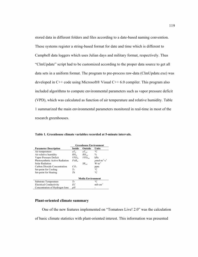
119
stored data in different folders and files according to a date-based naming convention.
These systems register a string-based format for date and time which is different to
Campbell data loggers which uses Julian days and military format, respectively. Thus
“ClmUpdate” script had to be customized according to the proper data source to get all
data sets in a uniform format. The program to pre-process raw-data (ClmUpdate.exe) was
developed in C++ code using Microsoft® Visual C++ 6.0 compiler. This program also
included algorithms to compute environmental parameters such as vapor pressure deficit
(VPD), which was calculated as function of air temperature and relative humidity. Table
1 summarized the main environmental parameters monitored in real-time in most of the
research greenhouses.
Table 1. Greenhouse climate variables recorded at 5-minute intervals.
Greenhouse Environment Parameter Description Inside Outside Units Air temperature aTin aTout °C Air relative humidity RHin RHout % Vapor Pressure Deficit VPDin VPDout kPa Photosynthetic Active Radiation PARin mmol·m-2·s-1 Solar Radiation SRout W·m-2 Carbon Dioxide Concentration CO2 ppm Set-point for Cooling Tc °C Set-point for Heating Th °C Media Environment Substrate Temperature Ts °C Electrical Conductivity EC mS·cm-1 Concentration of Hydrogen Ions pH -
Plant-oriented climate summary
One of the new features implemented on “Tomatoes Live! 2.0” was the calculation
of basic climate statistics with plant-oriented interest. This information was presented
120
graphically as part of the monitoring system, and the numerical values were also
available as text files.
It has been reported in the literature the direct correlation between the total
accumulated light and plant growth/yield, for different long-term greenhouse crops such
as tomatoes, peppers, and cucumbers (Bruggink, 1987); and control strategies for
consisting daily integrals in short-term greenhouse crops (lettuce) have been developed
already (Albright et al., 2000).
Although solar radiation is one of the main factors defining yield, not much control
is applied, except when it is excessive (summer) shade curtains or paints on the glazing
may be implemented. In contrast, during periods of low solar radiation such as winter,
supplemental light may be implemented. Due to the inability to control the incoming
solar radiation to a desired optimum, other control measures are applied to compensate
for this deficiency and produce an optimum plant response under the resulting
greenhouse environment. These control strategies may include the level adjustment of:
the CO2 supplementation, the EC on the nutrient solution, the watering frequency, and the
air temperature (Jensen, 2002).
Greenhouse air temperature is highly dependent on the incoming solar radiation, and
it is the main environmental parameter controlled. Its control is implemented as a crop
blueprint (set-point) for each of the greenhouse actuators (vents, fans, heaters, foggers,
shade curtains). The control schemes are defined for daytime (aTinD), nighttime (aTinN) or
more recently as a 24-hour (aTin24) average air temperature. Air temperature control is
based on its effect on plant growth (stem elongation), as reported in young tomato plants
121
(Heuvelink, 1989) and other greenhouse crops (Bertram and Karlsen, 1994) when
different day and night temperature regimes are implemented. This follows the concept of
DIF, the difference between day temperature (aTinD) and night temperature (aTinN) (DIF =
aTinD - aTinN). A new control scheme based on the temperature integration concept
(Korner and Challa, 2003a), has been implemented for process-based humidity control
(Korner and Challa, 2003b), and for energy consumption reduction (Korner et al., 2004).
After air temperature, the second most important parameter controlled is water
content within the greenhouse environment, which is affected by the water transpired
from the plants, the water evaporated from the ground, irrigation and cooling systems,
and the water lost by ventilation. Humidity has a different effect on each crop, and at
each crop stage. In low humidity conditions (dry hot climates) leaf stomata are closed to
avoid water stress, photosynthesis is reduced, and canopy temperature increases, having
all negative effects in plant growth and yield. In contrast, higher humidity levels not only
results in problems with fungal diseases, but also with low crop transpiration due to low
VPD, which may result in nutrient deficiencies (such as calcium) (Jolliet, 1999). Vapor
pressure deficit (VPD) is a better indicator for disease threat, condensation potential, and
the transpiration in greenhouse crops. The effect of different levels of VPD during the
day and at night have a significant effect on tomato yield (Jolliet, 1994).
The plant-oriented environmental parameters calculated and included in the
monitoring system were: 1) daily light integral (MJ m-2 d-1 or mmol·m-2·s-1, depending on
the greenhouse sensor), 2) average air temperature (°C) for daytime (aTinD), nighttime
(aTinN), daily (aTin24), and DIF, 3) average relative humidity (%) for daytime (RHinD),

122
nighttime (RHinN) and daily (RHin24), and 4) average VPD (kPa) for daytime (VPDinD),
nighttime (VPDinN) and daily (VPDin24).
To compute daytime or nighttime averages and derived or integrated parameters for
daily climate statistics, algorithms to determine sunrise and sunset times and day lengths
were implemented. Sunset and sunrise time values were calculated as function of day of
the year (Julian day) and geographic location.
The script to generate the daily climate summaries (“clmSummary”) ran at 24-hour
intervals, and was executed after midnight.
A graphical representation of the plant-oriented climate parameters calculated for a
greenhouse tomato crop (season 2007-2008) is shown in Figure 3.
Integrated daily solar radiation (Figure 3A) varies as a function of the day of the year.
While during the summer there were values of around 20 to 25MJm-2d-1, in winter there
was only 15 MJm-2d-1, which resulted in lower productivity.
The main environmental parameter controlled was air temperature (Figure 3B) which
was controlled consistently to daily averages (aTin24) at 20 °C (in fall) and 18 °C (in
winter). The performance of the climate controller in following the set-points for daytime
and nighttime was good as shown with the average air temperature for daytime (aTinD)
and nighttime (aTinN). A positive DIF (~ 7 °C) was maintained trough the crop season.
Relative humidity (Figure 3C) on average was controlled on the 40 to 60 % range.
VPD (Figure 3D), although not routinely controlled, was maintained in the range of 0.6
to 1.5 kPa which is a good level for growing greenhouse crops.

123
270 290 310 330 350 5 25 450
10
20
30S
olar
Rad
iatio
n (M
J m
-2 d
-1)
A
SR .
270 290 310 330 350 5 25 450
10
20
30
Air
Tem
pera
ture
( °C
)
B
aTin24
aTinD
aTinN
DIF
270 290 310 330 350 5 25 4520
40
60
80
100
Rel
ativ
e R
umid
ity (
% )
C
RHin24
RHinDRHinN
270 290 310 330 350 5 25 450
0.5
1
1.5
2
Julian Day
VP
D (
kPa
)
D
VPDin24
VPDinDVPDinN
Figure 3. Plant-oriented climate parameters of a greenhouse crop (2007-2008).
Data storage and backup
Continuous collection of data generated large data files. To avoid large files the
third script (“ClmBackup”) running at 7-day intervals refreshed the text files where the
dedicated PCs stored new records. Data was stored locally and remotely in a folder
structure following a “Greenhouse Name/wk_week of year” naming format and in 7-day
124
intervals. These files could also be accessed online for further analysis and
implementation on concurrent research projects.
User interface
The user interface, implemented as a Web-based application, allowed faculty,
researchers, students, and the general public to access all the components of the
greenhouse monitoring system through a Web page (http://ag.arizona.edu/ceac/live2/)
hosted at the HTTP server of the College of Agriculture and Life Science. This server
operated under a UNIX platform, and had the capability of handling multiple clients
accessing the same web pages (data) at the same time in a fast and reliable way. The main
page of “Tomatoes Live 2.0” included links to each of the research greenhouses and to a
Web page of real-time images of all greenhouses.
The components of the monitoring system, available to each of the greenhouses,
included: 1) real time data of the parameters of interest in tabular format, 2) graphics of
the data from the past 24-hour interval of the previous parameters, 3) real time images of
the crop, 4) graphics of the data from the past 7-day interval, 5) graphics of the climate
data summary, and 6) access to data older than 7 days stored in coma separated text files.
A plotting tool was developed using the Java™ programming language to present
numerical data graphically. This plotting tool was embedded as Java Applets on each of
the Web pages of the monitoring system. An image in Figure 4 includes several
components of the user interface including: real-time data, real-time crop images,
graphics of 24-hour data, buttons to access other data or to monitor other greenhouses.

125
Figure 4. User interface of the greenhouse monitoring system. Near real-time data, real-time crop images and plots of historical data in a 24-h period of one research greenhouse are displayed.
GENERAL DISCUSSION
The upgraded greenhouse monitoring system “Tomatoes Live! 2.0” could be
accessed through the Web page of the Controlled Environment Agriculture Center
(http://ag.arizona.edu/ceac/), allowing for the remote monitoring of the production of
greenhouse crops. This system was implemented on a greenhouse educational laboratory

126
and on several research greenhouses in the CEAC. The current system integrates the
outputs of different greenhouse climate controller software and data loggers, and displays
in near real-time graphs and numerical values of parameters of interest in controlled
environment agriculture.
Greenhouses are structures aimed to provide optimum environmental (aerial and root
zone) conditions for increased crop yield while making efficient use of resources. The
most popular parameters monitored include: air temperature, relative humidity, VPD,
CO2, and PAR (Table 1 and Figure 4). Some research units include the automated
monitoring of root zone conditions such as EC, pH, and substrate temperature.
The greenhouse monitoring system has proved to be a practical educational tool and
has been continuously used in several classes within the CEA program. These classes
(PLS217, PLS394, PLS475A, ABE483 and ENTO497C) cover several topics related to
greenhouse hydroponic crop production, physiology of plants under controlled
environments, greenhouse pest management and greenhouse engineering. In these classes
the students could oversee the current status of the crop and the operation of the physical
system. Furthermore, researchers, support staff, and even research granting agencies
could independently observe the operations and the crop response from remote locations.
For research purposes “Tomatoes Live!” has allowed researchers and faculty
working on collaborative projects to oversee the greenhouse operations and to have
access to real-time and historical data without time, spatial or software constrains;
allowing them to make decisions accordingly to the status of the crop. The multi-user
architecture of the system allowed monitoring the performance of the greenhouses by
127
many people, where several research experiments are conducted. This was especially
critical whenever a system failed to maintain the expected environmental conditions.
The prompt detection of failures on any of the components within greenhouse crop
production systems is always critically important, due to the risk of losing a crop or
experiment within a few hours or minutes, depending on the environmental situation and
on the specific failure of the control systems. Although greenhouse systems include
environmental alarms for failure of critical systems, the enhanced ability of remote
human monitoring has dramatically improved the resolution of determining off-nominal
conditions, thereby providing for greater foresight into problems as they develop.
Furthermore, having a web-based monitoring tool provides easy access to many
interested parties to help oversee the status of the system at any time from anywhere,
thereby significantly improving the climate conditions for the crops.
Examples of some of the systems failures that have been detected with the web-
based monitoring system include: 1) ventilation inlet openings that failed to open during
cooling mode, resulting in an increased greenhouse air temperature exceeding 50 °C
within less than 10 minutes, 2) in nighttime winter, when the outside climate conditions
were less than 4 °C, the heater’s capacity did not meet the heat load required to reach the
set-point of air temperature; although plants were not at risk, it showed that the system
could not perform well under those conditions, and 3) unusual sensor values that indicate
faulty sensors or the need to be calibrated or re-positioned for more accurate
measurements.

128
Although visual inspection of the plants is possible with the cameras, it is limited to
the resolution, current light conditions, and the manipulability of the cameras. Additional
information about the crop that climate data and images do not provide, is required in
order for the system to provide complete information of the status of the plant-
greenhouse system which then could be used for remote diagnosis by telepresence.
Additional information includes plant and fruit morphological and physiological features.
Currently some of the morphological properties are manually recorded but in the future
could be integrated with the web-based monitoring system by using a compatible data
base system, or possibly with additional sensors that have yet to be developed.
FINAL REMARKS
“Tomatoes Live!” 2.0 enabled a way for near real-time monitoring of greenhouse
plant production systems through any device (computer or mobile device) with access to
the Internet, without having temporal or spatial limitations. It has proved to be valuable
not only in academia and other collaborative research projects, but also as a potential tool
for remote diagnosis in large production systems where qualified staff was limited or in
production systems located in remote and/or hostile environments such as the South Pole.
The system has been reliable and continually operating since its initial implementation in
2001.
Acknowledgements
This research was initially funded by the Small Grant Program of the University of
Arizona and further developed with financial support from CEAC for equipment

129
acquisition. Special thanks to Neal Barto and Stephen Kania for hardware installation at
each of the greenhouses.
REFERENCES
Aaslyng, J.M., N. Ehler, and L. Jakobsen. 2005. Climate control software integration with a greenhouse environmental control computer. Environmental Modelling & Software. 20: 521-527.
Aaslyng, J.M., J.B. Lund, N. Ehler, and E. Rosenqvist. 2003. IntelliGrow: a greenhouse component-based climate control system. Environmental Modelling & Software. 18: 657-666.
Albright, L.D., A.-J. Both, and A.J. Chiu. 2000. Controlling greenhouse light to a consisting daily integral. Transactions of the ASAE. 43: 421-431.
Bertram, L.and P. Karlsen. 1994. A comparison study on stem elongation of several greenhouse plants. Scientia Horticulturae. 59: 265-274.
Bruggink, G.T. 1987. Influence of light on the growth of young tomato, cucumber and sweet pepper plants in the greenhouse: Calculating the effect of differences in light integral. Scientia Horticulturae. 31: 175-183.
Chikwamba, R., J. McMurray, H.X. Shou, B. Frame, S.E. Pegg, P. Scott, H. Mason, and K. Wang. 2002. Expression of a synthetic E-coli heat-labile enterotoxin B sub-unit (LT-B) in maize. Molecular Breeding. 10: 253-265.
Choi, C.Y., E. Fitz-Rodriguez, and G.A. Giacomelli. 2002. Web based monitoring in controlled environment agriculture. ASAE -CIGR Congress Annual International Meeting, Chicago IL, USA, July 29-31.
Ehler, N. 1991. Interfacing crop models to standard software for greenhouse climate control. Ecological Modelling. 56: 245-257.
Ehler, N.and J.M. Aaslyng. 2001. Real-time monitoring of greenhouse climate control using the internet. HortTechnology. 11: 639-643.
Ehret, D.L., A. Lau, S. Bittman, W. Lin, and T. Shelford. 2001. Automated monitoring of greenhouse crops. Agronomie. 21: 403-414.
Fitz-Rodriguez, E., C. Kubota, C. Pagliarulo, and G. Giacomelli. 2003. Asynchronous education in controlled environment agriculture. World Conference on E-Learning in Corporate, Government, Healthcare, and Higher Education 2003, Phoenix, Arizona, USA. p. 72-75.
Giacomelli, G.A., R.L. Patterson, and P.D. Sadler. 2007. Telepresence technologies and practices for enabling remote semi-autonomous CEA food production. Acta Hort. (ISHS). 761: 21-31.

130
Heuvelink, E. 1989. Influence of day and night temperature on the growth of young tomato plants. Scientia Horticulturae. 38: 11-22.
Jensen, M.H. 2002. Controlled environment agriculture in deserts, tropics and temperate regions -A world review. Acta Hort. (ISHS). 578: 19-25.
Jolliet, O. 1994. HORTITRANS, a model for predicting and optimizing humidity and transpiration in greenhouses. J. agric. Engng. Res. 57: 23-37.
Jolliet, O. 1999. Water cycle, p. 303-326. In: H. Zvi Enoch (ed.). Greenhouse ecosystems 20. Elsevier.
Korner, O., M.J. Bakker, and E. Heuvelink. 2004. Daily temperature integration: a simulation study to quantify energy consumption. Biosystems Engineering. 87: 333-343.
Korner, O.and H. Challa. 2003a. Design for an improved temperature integration concept in greenhouse cultivation. Computers and Electronics in Agriculture. 39: 39-59.
Korner, O.and H. Challa. 2003b. Process-based humidity control regime for greenhouse crops. Computers and Electronics in Agriculture. 39: 173-192.
Lopes, A.A., S.M. Paz, C.E. Cugnasca, and A.M. Saraiva. 2002. Sharing video images on the Internet using Java: An application to controlled environment. Procedings of the World Congress of Computers in Agriculture and Natural Resources, Iguacu Falls, Brazil, March 13-15. p. 114-118.
Morais, R.and J. Boaventura Cunha. 2000. Agritronics: a distributed data acquisition and control network for agricultural environments. Acta Hort. (ISHS). 534: 319-325.
Sijmons, P.J., A.J.J. Van Ooiijen, and A. Hockema. 1993. Protein production in transgenic crops: Analysis of plant molecular farming, p. 241-250. Industrial crop production. Elsevier, Amsterdam.
Stevens, G., E. Vories, M. Mulesky, M. Rhine, and D. Dunn. 2007. Irrigation to maximize vaccine antigen production in genetically modified tobacco. Agronomy Journal. 99: 1271-1277.
USDA. 2002. The Census of Agriculture Vol. 2008, National Agricultural Statistics Services.
131
APPENDIX C: YIELD PREDICTION AND GROWTH-MODE CHARACTERIZATION OF GREENHOUSE TOMATOES WITH NEURAL NETWORKS AND FUZZY LOGIC
E. Fitz-Rodríguez, G. A. Giacomelli
Department of Agricultural and Biosystems Engineering, University of Arizona Tucson, AZ.
132
ABSTRACT.
Despite the technological advances implemented in greenhouse crop production, its
operation relies on human expertise to decide the optimum values of each environmental
control parameter. Most importantly the selected values are determined by human
observation of the crop responses. Greenhouse tomatoes often show a pattern cycling
between reproductive and vegetative growth-modes. The growth-mode is a practical
visual characterization of the source-sink relations of the plants resulting from the
greenhouse environment (aerial and root zone). Experienced greenhouse tomato growers
assess the growth-mode based on morphological features, including quantitative (length,
diameter, elongation rates) and qualitative (shape and color) of the plant head, stems,
flowers, trusses, and leaves. Data from greenhouse environments and crop records from
experimental production, located in Tucson, AZ., and from a large scale commercial
operation, located in Marfa, TX., were used for modeling the growth-mode of tomato
plants with fuzzy logic. Data from the commercial operation were implemented to model
weekly fluctuations of harvest rate, fruit size and fruit developing time with dynamic
neural networks (NN). The NN models accurately predicted weekly and seasonal
fluctuations of the fruit-related parameters, having correlation coefficients (R) of 0.96,
0.87 and 0.94 respectively for harvest rate, fruit fresh weight and fruit developing time,
when compared with a dataset used for independent validation. The fuzzy modeling of
growth-mode allowed the discrimination of reproductive and balanced growth-modes in
the experimental systems, and the seasonal growth-mode variation on the commercial
133
applications. Both modeling results are applicable to commercial operations for making
decisions on greenhouse climate control and overall crop management practices.
Keywords. Greenhouse tomato, Growth mode, Vegetative, Reproductive, Pattern
recognition, Dynamic neural network, Fuzzy logic, Modeling.
134
INTRODUCTION
The fresh tomato industry in North America (Canada, United States and Mexico) has
changed its dynamics since the early 1990s when tomatoes started to be grown in
greenhouses. In 2003 there were approximately 1726 ha of greenhouses dedicated to the
production of tomatoes and they provided for 37 % of the fresh tomato in the retail
market of the US (Cook and Calvin, 2005).
Sixty-five percent of the US domestic production is provided by four large-scale
greenhouse tomato growers for a total of 190 ha (Selina and Bledsoe, 2002). These
production systems are characterized by high technology, which includes the use of
hydroponic systems, computer climate control, carbon dioxide (CO2) supplementation,
and indeterminate plant cultivars. These technologies have combined to allow year-round
production, resulting in yields of more than 65 kg m-2 yr-1 (up to 15 times more than field
growers) and increased quality (90% of marketable fruits, in contrast to 40 to 60% in the
field) (Selina and Bledsoe, 2002).
Year-round production requires the use of greenhouse crops of long growing cycles.
These crops are characterized by a vegetative phase (starting at the seedling stage and up
to the appearance of the first inflorescence), and a continuous reproductive phase
(starting with flower development, pollination and fruit setting) that ends when the crop
is terminated. After the onset of the reproductive phase, both vegetative and reproductive
organs are continually developed, but it is well recognized that the plants cycle between a
“more vegetative” and “more reproductive” growth modes which are often characterized
by a very subtle plant physical and possibly physiological properties, which combine to

135
influence the amount and quality of near term yields as well as future yields. These
growth modes are qualitatively described as, vegetative, having a greater than desired
proportion of foliage mass to fruit mass, and reproductive, having the opposite, or greater
than desired proportion of fruit mass to foliage mass. There is no absolute ratio that is
always correct, but one of variable proportion of foliage and fruit that will depend on the
season of the year, the previous harvest rates, and other factors that combine to require a
specific ratio that will provide for maximum annual yields. This is determined by the
expertise of the grower. It is influenced directly by the crop management practices, and
by the aerial and root zone environment provided to the plant. An imbalance or a greater
direction towards one of these two growth modes result in lower than expected total
yields.
Despite the technological advances and the sophistication of greenhouse hydroponic
and climate control systems, greenhouse operation relies largely on human expertise to
decide the optimum values for each of the parameters of the plant-greenhouse system,
and most importantly, to verify by observation the desired response of the crop.
Experienced greenhouse tomato growers and researchers assess plant responses and
growth-mode, based on visual morphological observations of the plants. They use this
information for making decisions on climate control and crop management practices to
shift the plant growth towards a “balanced” growth mode with appropriate proportion of
vegetative mass to support the existing fruit load, and appropriate proportion of fruit load
to maintain desired yield and quality. Morphological observations include both
quantitative (length, diameter, elongation rates, etc.) and qualitative (shape, color)
136
features of the plant growing tip (head), stem, number of flowers and fruits, trusses, and
leaves (Jensen, 2004; Papadopoulos, 1991; Portree, 1996).
A recent study quantified plant growth status within several environments, as defined
by aerial and root zone environmental conditions, which successfully induced vegetative
and reproductive growth-modes in greenhouse tomato plants. The stem diameter (Sd) was
the morphological feature that showed the greatest response and sensitivity to the
environment. Plants within a reproductive inducing environment exhibited a thinner stem
diameter than those plants within vegetative inducing environments (Costa, 2007).
Tomato crop growth is a dynamic and complex phenomenon and it has been studied
through the development of mechanistic models. Two of the proven dynamic growth
models are TOMGRO (Jones et al., 1991; Jones et al., 1999) and TOMSIM (Heuvelink,
1996; Heuvelink, 1999). Both models are based on physiological (photosynthesis and
maintenance respiration) processes, and model biomass partitioning, growth and yield
(dry mass) as a function of numerous climate and physiological parameters. Their use is
limited, especially for practical application by growers, by their complexity and by the
difficulty to obtain the initial condition parameters required for implementation (Challa
and Heuvelink, 1996). Furthermore, destructive measurements are required for
calibration and validation for each application.
Although less complex greenhouse tomato models to predict yield currently exist,
they are limited in the results provided, and have an inconsistency to predict long-
production cycles. Furthermore of the parameter calibration is required under new
conditions. TOMPOUSSE (Abreu et al., 2000) predicts yields in terms of number and
137
fresh weight of harvested fruits. This model was developed in France for heated
greenhouses and required the calibration of the linear relationships of both, flowering rate
and fruit growth period, with air temperature when implemented in unheated plastic
greenhouses in Portugal. The model performed poorly, in lieu of simplicity, and was only
tested for short production cycles of less than fifteen weeks of production.
Another greenhouse tomato model proposed by Adams (2002), implemented on a
graphical simulation tool (HIPPO), focused on explaining the weekly fluctuations of
greenhouse tomato yields as characterized by fruit size and harvest rates. This model
required hourly climate data for determining the rates of leaf, truss and flower production.
Even though the seasonal fluctuations of yield in greenhouse crops is well
understood as being influenced by the seasonal variation of solar radiation and air
temperature, greenhouse growers are also interested in the short and long term
fluctuations of yield and quality of the crop. Crop models that predict harvest rates and
produce quality are useful tools that could help growers in making short and long term
decisions, for example, in defining climate control strategies, in synchronizing crop
production with marked demands, in managing labor force, in developing marketing
strategies, and in maintaining a consistent year-round produce quality.
Neural networks and fuzzy logic offer the advantage of modeling nonlinear
relationships and add robustness in situations of imprecise and incomplete data, where
uncertainty exists. Some application examples are in the areas of forecasting, control,
optimization, and pattern recognition. Intelligence is added to the process by computing
the degree of uncertainty, and computing with linguistic terms (fuzzy variables). More
138
accuracy is obtained compared to mechanistic models, furthermore the amount of
parameters used to describe the system behavior are reduced.
There have been numerous studies applying either, neural networks or fuzzy logic in
greenhouse production systems. Most of them are focused on modeling the air
temperature in greenhouse environments (Frausto et al., 2003; Linker and Seginer, 2004;
Seginer, 1997; Seginer et al., 1994), or for optimal control of CO2 (Linker et al., 1998)
with neural networks. Recent techniques have included modeling the greenhouse
environment with hierarchical fuzzy modeling (Salgado and Cunha, 2005), or controlling
the environment with optimized fuzzy control (Ehrlich et al., 1996; Lafont and Balmat,
2002). Fewer studies implementing computational intelligence (CI) techniques for plant
modeling have been reported. Tien (1997) implemented a hybrid Neuro-Fuzzy approach
for the system identification and modeling of the total dry weight yield of tomato and
lettuce. Center and Verma (1997) developed a fuzzy model to predict net photosynthesis
of tomato crop canopies, and the results were highly correlated to the outputs of the
mechanistic model TOMGRO to model crop processes. Pucheta el al. (2005)
implemented Neuro-dynamic programming for the greenhouse optimal control for tomato
seedlings production. Ehret et al. (2008), used artificial neural networks to predict cuticle
cracking in greenhouse peppers and tomatoes.
The current research proposes the implementation of computational intelligence
techniques, and in particular dynamic neural networks for modeling and predicting
weekly harvest rates, and fuzzy logic for growth-mode characterization of greenhouse
tomatoes plants. The objectives of this study were to investigate the use of computational
139
intelligence techniques that could be implemented with current crop and climate records
from greenhouse growers, by implementing:
1. Computational neural networks for weekly yield prediction of greenhouse tomatoes
from environmental and crop related variables. Where yield was characterized by
yield per unit area, Ya (kg m-2), fruit fresh weight, FRg (g), and fruit growth period
SHd.
2. Fuzzy logic for characterizing plant growth mode (vegetative, balanced, or
reproductive) in greenhouse tomato plants as a function of plant morphological
features (stem diameter and truss height).
MATERIALS AND METHODS
Crop records and climate data
Crop records and climate data from a large scale 32.4 ha greenhouse tomato
operation located in Marfa, Texas, U.S. were used for designing and training
computational neural networks for yield prediction and for implementing a fuzzy
inference system for plant growth-mode characterization. These data included six data
sets from two production cycles (S1: 2002-2003 and S2: 2003-2004) and four
greenhouses (GH1, GH2, GH3, and GH4). Additional data sets from experimental trials
were used to derive the fuzzy inference system (FIS) for plant growth-mode
characterization. These experimental trials provided environmental conditions for
inducing reproductive and vegetative growth-modes on greenhouse beefsteak tomato
plants cv. ‘Rapsodie’ which were grown at the Controlled Environment Agriculture
140
Center (CEAC) of the University of Arizona in Tucson, AZ (Costa, 2007). Planting dates
and crop growth periods for both datasets are summarized in table 1.
Tomato on the vine (TOV) plants (cv. ‘Clarence’) and beefsteak tomatoes (cv.
‘Quest’) were grown in the commercial operation within Venlo-type glass greenhouses
on a high wire system with rockwool hydroponic substrate, CO2 supplementation, and
computer climate/irrigation control. The greenhouses were equipped with hot water
heating pipes, and roof vents for passive cooling. Plant density of the crop was 2.7 plants
m-2 and crop maintenance, including fruit pruning to 4 or 5 fruits per truss, shoot removal,
and deleafing were performed weekly.
Crop records, provided by the grower, included weekly measurement of 26 plant
morphological features, as described on table 2. Crop records included twelve plant
samples per greenhouse, which were randomly selected and continuously measured
during the production cycle.
Daytime, nighttime and 24-hour averages of daily climate data from the outside and
the inside of the greenhouse were also provided. Weekly averages were computed to
match the weekly records of the crop (Table 3).
The outside climate conditions of the greenhouse locations are summarized in Figure
1, where solar radiation is excellent for year-round production, and that greenhouse air
temperature control could be achieved with passive cooling for most of the year, except
in the June-August period where the 24-hour average air temperature approached 25 °C
requiring artificial cooling.
141
Three parameters were modeled and predicted by means of neural networks:
1. Yield (Ya, kg m-2 week-1), which is of interest for greenhouse grower for
developing short term crop management strategies. Also, it is useful for
developing long term marketing and labor management strategies. As previously
reported, greenhouse tomato cumulative yield can be described with a direct
linear relationships to cumulative solar radiation, either as fresh weight
(Cockshull, 1988) or dry mass (Heuvelink, 1995). Although these results were
important to describe the overall effect of solar radiation on yield and for
validating mechanistic models, respectively. Both studies were performed in
northern latitudes, without CO2 enrichment, for short production periods (<100
days), and plants were cultivated in soil, not hydroponically. These are not current
standard cultivation methods of most of the greenhouse growers implementing
high technology production. In Figure 2 the cumulative weekly yield for full
production cycles (>35 weeks of harvest) is shown as a function of cumulative
solar radiation for each data set. The results also show a linear relationship.
2. Fruit size expressed as fresh fruit weight, FRg (g), which is a direct indicator of
the produce quality according to the marketing grading standards, and it is also an
indirect indicator of tomato taste quality, as 50 % of the fruit dry matter content
are soluble solids and fruit dry matter represents from 4 to 8% of the fruit fresh
weight (Heuvelink and Dorais, 2005).
3. Fruit growth period, SHd (d), the time it takes a fruit to develop from anthesis to
harvest. It is used as a reference to fruit development as influenced mainly by fruit
142
temperature. This parameter is inversely related to fruit development rate and
shows a linear relation with air temperature (Heuvelink, 2005; Heuvelink and
Dorais, 2005). This relationship is shown in Figure 3 for SHd of all the dataset,
which had a correlation coefficient R=0.94 with air temperature Tin24 when
integrated over the same growth period. Degree-days is another predictor of fruit
growth period, and for greenhouse tomatoes it has been reported to be 940 degree-
days when using a base temperature of 4 °C (de Koning, 1994). The sum of
degree-days for each harvested cluster was calculated for each dataset and in
Figure 4, the values fluctuates between 800 and 970 °C d during the production
cycle.
Neural network model
Computational neural networks (CNN) have proved to be a powerful tool to solve
several types of problems in different fields where approximation of nonlinear functions,
classification, identification and pattern recognition are required. Neural networks are
mathematical representations of biological neurons in the way they process information
as parallel computing units. In general there are two types of neural network
architectures: 1) static (feedforward), where no feedback or time delays exists, and 2)
dynamic neural networks, whose outputs depend on the current, or previous inputs,
outputs or states of the network (Demuth et al., 2007).
One of the most widely used neural network architectures is the multilayer
perceptron (MLP), which has been proved to approximate almost any continuous
function over a compact subset of Rn, if given enough hidden layers and neurons within
143
them (Master, 1993). Its mathematical proof, based on the Stone-Weierstrass theorem,
can be found in Gupta et al. (2003), and it has also been studied by many other authors
such as (Blum and Li, 1991; Hornik, 1991). A MLP is a structure mapping an input space
Rn into an output space Rm, by adjusting the connection weights, linking each of the input
elements to the neurons in the hidden layers and throughout the output layer. Finding the
appropriate number of hidden layers, neurons within each layer, and weight adjusting
methods, constitute the neural network design procedure. Finding a combination of these
that best approximates the problem solution is a heuristic process that depends on the
problem and type of data being processed.
Input /output parameters
The architecture and training mode of the neural network depends on the inputs and
output parameters of the problem being solved. The tomato crop includes biological
entities that show a nonlinear dynamic behavior and its response depends not only on
several environmental (aerial and root zone) factors, but also on the current and previous
crop conditions, as the source-sink strengths are modified. Greenhouse tomatoes have
long production cycles and the growth and development of leaves, stems and fruits
(sources and sinks) happen concurrently and continuously.
The effects of several environmental factors (light, CO2, air humidity, and air
temperature) have both a short and long term impact on the source-sink strengths within
tomato plants. Air temperature is the most influential parameter that allows biomass
partitioning as it directly affects fruit growth (Heuvelink and Dorais, 2005). Even though
greenhouse air temperature is controlled to an optimum, greenhouse tomatoes have a
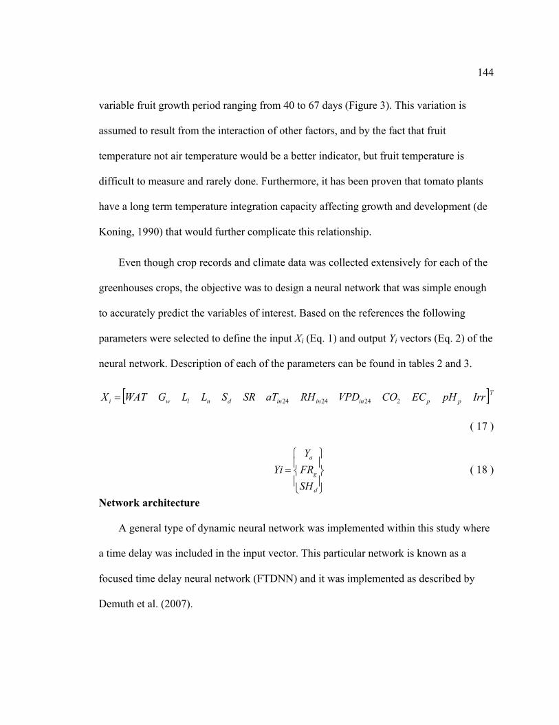
144
variable fruit growth period ranging from 40 to 67 days (Figure 3). This variation is
assumed to result from the interaction of other factors, and by the fact that fruit
temperature not air temperature would be a better indicator, but fruit temperature is
difficult to measure and rarely done. Furthermore, it has been proven that tomato plants
have a long term temperature integration capacity affecting growth and development (de
Koning, 1990) that would further complicate this relationship.
Even though crop records and climate data was collected extensively for each of the
greenhouses crops, the objective was to design a neural network that was simple enough
to accurately predict the variables of interest. Based on the references the following
parameters were selected to define the input Xi (Eq. 1) and output Yi vectors (Eq. 2) of the
neural network. Description of each of the parameters can be found in tables 2 and 3.
[ ]Tppininindnlwi IrrpHECCOVPDRHaTSRSLLGWATX 2242424=
( 17 )
⎪⎭
⎪⎬
⎫
⎪⎩
⎪⎨
⎧=
d
g
a
SHFRY
Yi ( 18 )
Network architecture
A general type of dynamic neural network was implemented within this study where
a time delay was included in the input vector. This particular network is known as a
focused time delay neural network (FTDNN) and it was implemented as described by
Demuth et al. (2007).
145
The neural network model was implemented using the Neural Network Toolbox™
5.1 of Matlab® 7.5 (The MathWorks, Inc., Boston, MA, USA). The general architecture
of the FTDNN is represented in Figure 5, which consists of one input vector, two hidden
layers and a single output (Xi - HL1 -HL2- Yi). Three networks were designed and trained,
one for each of the parameters predicted (yield, fruit weight, and fruit developing time).
This dynamic network architecture was chosen because of its memory association and the
learning capability with sequential and time-varying patterns, which is the biological
situation for tomato plants.
FTDNN have a similar architecture to a static feedforward multilayer perceptron
(MLP), except for the input time delay. It could be trained with backpropagation
algorithms, and in the same way with gradient-descent algorithms.
Following the same notation found in Demuth et al. (2007) the output of the network
is computed as:
)))((( 3211,111,222,33 bbbpIWfLWfLWfY +++= ( 19 )
Where IW i,j and LW i,j represent the weight matrix of the input and hidden layers,
respectively. Superscripts (i, j) define the connection of the current layer (i) to the output
of the previous layer (j). b are the connection weights of the bias input in each layer. f are
the transfer functions (activation functions) in each of the layers, f 1 and f 2 were defined
as hyperbolic tangent sigmoid, whose range is bounded in the [-1 1] interval:
nn
nn
eeeea −
−
+−
= ( 20 )

146
and f 3is a linear transfer function defined as:
na = ( 21 ) FTDNN implement the time delay in the input vector (p) and it is defined as:
[ ]TDtttt XXXXp )()2()1()( −−−= L ( 22 )
where, T is the transpose, and the subscript (t-D) is the number of delays D (in this
case, D weeks of data).
The size of the weight matrix of the input layer (IW 1,1) is defined by the number of
neurons in the first hidden layer and the size of the vector p. The layer weights (LW i,j) are
defined in the same way as a MLP, and depend on the number of neurons in each layer.
Network training
The training process implies the iterative adjustment of the weights and biases of the
network by minimizing a performance function when presenting input and target vectors
to the network. The mean square error (mse), selected as the performance function, was
calculated as the difference between the target output and the network output.
∑∑==
−==Q
k
Q
kkakt
Qke
Qmse
1
2
1
2 ))()((1)(1 ( 23 )
Where, t(k) and a(k) represent the target vector and network output, respectively. Q
is the number of samples presented to the network. Weights and bias were adjusted by
implementing the Levenberg-Marquardt algorithm as described by Hagan et al. (1995).
Once defined the performance function and the learning algorithm, the number of
neurons in each of the hidden layers and the length of the input delay were defined

147
heuristically by systematically searching over different combinations. The combination
resulting with the minimum root mean square error was selected as the final network
architecture (Table 4).
Once established the network architecture, further training was performed to improve
the network performance. The network was incrementally trained by presenting the input
and output data as sequences. Four initial datasets (S1G1, S1G2, S2G1, and S2G4) of
TOV-type tomato plants were included in the training, testing and validation process and
a full dataset (S2G2), also of TOV-type tomatoes, remained unused for independent
validation.
The initial data sets were randomly divided, so that 60% of the samples were
assigned to the training set, 20% to the validation set and 20% to the test set.
Generalization in each of the networks was improved by implementing the early stopping
method through the validation set.
After training each of the networks to a satisfactory performance the independent
validation set (S2G2) was used to evaluate the prediction performance of the neural
networks and to present the results.
Fuzzy logic model
The plant growth-mode of the crop was assessed at each of the stages in the
production cycle, as it is an indicator of the source-sink strengths of the crop which
defines the resulting crop yield. These assessments were subjective and rely on the
experience of the grower. They are based on the inspection of several qualitative and
148
quantitative plant morphological features. Plant growth-mode is referred in a qualitative
way and is described with the non desired and extreme growth-modes, i.e. vegetative or
reproductive. A balanced growth-mode is defined as having morphological features with
values lying between the two extremes.
Fuzzy logic (FL) offers the advantage of evaluating imprecise data, it allows for the
implementation of general knowledge (i.e. growers experience) by using a natural
language (linguistic variables) through inferences systems capable of dealing with
uncertainty and where qualitative and quantitative features can be combined to model
complex systems. Fuzzy rule-based models are used in control systems, decision making,
and pattern recognition among many others. Further details of the theory, history and
applications can be found in fuzzy logic references (Buckley and Eslami, 2002; Piegat,
2001; Yen and Langari, 1999).
The characterization of plant growth-mode was investigated with fuzzy logic
modeling by implementing a fuzzy inference system (FIS) that maps measurable
morphological features into plant growth-modes. The growth-mode is a qualitative
feature and it is expressed as a linguistic variable which includes a descriptive term and a
numerical value representing the degree of membership to a fuzzy set.
Most of the morphological features are qualitative and are difficult to record and to
make clear calculative decisions with these, however, experienced growers make
inferences with them to adjust the operation of the whole systems with huge financial
consequences. Two of the measurable morphological features that are most implemented
in commercial operations are: 1) stem diameter (Sd) – defined as the diameter of the plant
149
stem at 15 cm below the growing tip of the plant (apical meristem), and 2) truss height
(Th) – defined as the distance to the first open flower from the apical meristem were used
in a FIS.
Plants can be characterized as having a reproductive, balanced, or vegetative growth-
mode which were expressed as a function of the two previously mentioned morphological
features Sd and Th. A thin stem diameter is characteristic of a reproductive growth-mode.
In contrast thick stem diameters characterize a vegetative growth-mode. Meanwhile, a
balanced growth-mode has been learned by experience to have approximately a 10 mm
stem diameter. Similarly, truss height that is less than 10 cm is characteristic of
reproductive growth, while balanced growth-mode is defined with truss height in the
range from 10 to 15 cm, and finally a truss height greater than 15 cm defines a vegetative
growth-mode. These ranges were similar to those reported in the literature (Jensen, 2004;
Papadopoulos, 1991; Portree, 1996), as well as within experimental research trials
reported by Costa (2007). These numerical ranges are not exact and are most likely
cultivar, seasonal and geographically dependent. These slight differences can be
accounted for by the fuzzy logic which is robust with imprecise data.
The steps for the development of the FIS included: 1) Fuzzify the inputs/outputs
parameters, by defining the term sets and hedges for each of the input (Sd and Th) and
output (growth-mode) variables, and assign the membership functions to each fuzzy set;
2) define the fuzzy if-then rules, by application of the fuzzy operators on the antecedent
and the definition of an implication method; 3) define an aggregation method for
150
integrating all the outputs from the if-then rules, and 4) define a defuzzification method
to return a numeric value associated to a fuzzy set (qualitative feature).
The morphological features resulting from the experimental trials described by Costa
(2007) were used to define the universe of discourse (X) and the possibility distributions
(Figure 6 and Figure 7) defining each of the membership functions (Figure 8a and 8b) of
the fuzzy sets for the input parameters of the FIS. A Mamdani-type FIS was implemented,
where the outputs are defined also as fuzzy sets.
The universe of discourse for growth-mode was defined in a range from 0 to 10. A
hedge, “very”, was applied to the reproductive and vegetative growth-modes resulting in
five membership functions (Figure 8c). VR represents a “very reproductive” growth
mode, R a “reproductive”, V a “vegetative” growth mode and VV a “very vegetative”
growth-mode.
A fuzzy set A defined in a universe of discourse X, whose elements are denoted by x,
is defined as a set of ordered pairs.
}|)(,{ XxxxA A ∈= μ ( 24 )
Where μA(x) is the membership function (MF) of x in A, mapping each element into
a membership value between 0 and 1. The membership functions implemented were
Gaussian-type symmetric and double MF combined in the extreme values (Figure 8).
The inference system was defined with fuzzy if-then rules (table 5), mapping the
input variables into the new fuzzy variables defined for the growth-mode. Although the
antecedents of the fuzzy rules may combine multiple simple conditions, given by the two
151
inputs, it was selected to draw conclusions on each of the variables independently, given
by the natural non-existing conditions of having plants with thin Sd and long Th, or having
thick Sd and short Th, for stem diameter and truss height, respectively (table 6). Each rule
was evaluated in parallel, and assigned a weight of one.
The integration of the fuzzy sets representing the outputs of each of the if-then rules
was aggregated with the maximum operator, resulting in a fuzzy set describing the
growth-mode. Finally, the numeric value representing the degree of growth-mode (in a
numerical scale from 0 to 10) was calculated by defuzzifying the fuzzy set resulting in
the aggregation process with the centroid method. The FIS to characterize plant growth-
mode was implemented using the graphical interface of the Fuzzy Logic Toolbox™ Ver.
2.2.6 of Matlab ® 7.5 (The MathWorks, Inc., Boston, MA, USA).
RESULTS AND DISCUSSION
The results are presented in two sections. The first includes the results of modeling
and predicting fruit-related parameters with dynamic neural networks. The second
describes the results of modeling and characterizing the growth-mode of greenhouse
tomatoes plants with fuzzy logic.
Neural network modeling
The greenhouse environment achieved/applied in one of the greenhouses (S2GH2)
from a commercial operation is shown in Figure 9. Greenhouse air temperature,
expressed as 24-hour average, is the main environmental parameter controlled. It has a
seasonal variation ranging from approximately 25 °C during summer and decreasing to
152
approximately 18 °C during winter and early spring. Controlling air temperature also
affects other parameters such as air humidity and CO2 concentration levels.
Weekly and seasonal variations in the production were observed within three fruit-
related parameters, including: 1) Ya, weekly harvest rates (kg m-2 week-1) that fluctuated
from 0.78 and 1.6 for 10 weeks, and then fluctuated near 1.0 during the next 25 weeks of
production; 2) FRg, fresh fruit weight (g), indirectly expressing fruit size with weights
ranging from 153 to 174 g with no specific pattern; and 3) SHd, fruit growth period (d)
whose values increased from 40 to 64 days during the production cycle, in a non-
consistent pattern. These parameters, shown in the “Sample” datasets in Figure 10, are of
interest for making decision on the greenhouse operations, on crop and labor
management and on maintaining a consisting produce quality.
The inputs of the model (equation 1), parameters currently recorded by most of the
growers, included: 1) plant oriented observations (WAT, Gw, Ll, Ln, and Sd) which
embedded morphological features of plant development, 2) greenhouse aerial
environment (SR, aTin24, RHin24, VPDin24, and CO2) and 3) root zone environment (ECp,
pHp and Irr). It was assumed that the environment applied throughout the production
cycle was the optimum at every stage of the crop for achieving increased yield at the
lowest production cost. This assumption is based on the experience of the grower whose
yield surpassed 65 kg m-2 per year for the current datasets. Recent data not included in
this study reported a total annual production of 94 kg m-2 (HortiMax, 2008). Based on this
assumption, the resulting environment was used as the input parameters to model and
predict the fruit-related variables.
153
The proposed dynamic network architectures (table 4) performed well in modeling
and predicting each of the fruit-related parameters with the validation dataset, as well as
with the dataset (S2GH2) used as an independent validation (Figure 10). A regression
analysis between the predicted values by the neural network model and the corresponding
measured values for the independent dataset resulted in correlations coefficients (R) of
0.96, 0.87 and 0.94 for harvest rate, fruit size and fruit developing time, respectively. The
correlation coefficients and overall root mean square error (RMSE) for the measured and
predicted values on each of the parameters indicates the good performance of the neural
networks (table 4). Each of the trained networks predicted well not only the overall
seasonal variations, but also the weekly fluctuations.
Except for the recent work reported by Ehret et al. (2008), where data from
commercial operations were used to design and train neural networks to predict cuticle
cracking in tomatoes and peppers, no other results have been reported in the literature
that implements datasets from full crop production cycles from commercial operations.
The current study is also one of the first modeling studies implementing neural
networks to model and predict fruit-oriented parameters (Ya, FRg and SHd) for year-round
production cycles with standard management practices at large scale commercial
operations. Although the resulting neural networks models are capable of predicting the
seasonal and weekly variations of the fruit-oriented parameters, they do not provide a
mechanistic explanation of the factors influencing these fluctuations. However, knowing
this information in advance could be valuable for growers for making decision on climate
and crop management.

154
Some of the advantages of the NN model implemented include: 1) the input
parameters of the model are currently recorded by most growers which make it easy to be
implement, 2) the NN model could “learn” from datasets with new scenarios (new
cultivars, different control strategies, improved climate control, etc), and 3) less
experienced growers could use the system, where the decision making process of the
most experienced growers was captured by the data used in the trained networks, and the
production could become more consistent.
Fuzzy modeling
The growth-mode of greenhouse tomato plants was modeled and characterized with
fuzzy logic. The resulting FIS allowed the characterization of two types of tomatoes
including TOV and beefsteak. These crops were grown under experimental trials and
under standard commercial operations.
Data from the experimental trial, which included only beefsteak tomatoes cv.
‘Rapsodie’, were used for deriving the FIS. The resulting growth-mode characterization
for each treatment in the experimental trial is shown in Figure 11. Although environments
for inducing vegetative growth-modes (VPDLow and EC=2.5) were applied, plants did not
achieved a truly vegetative growth-mode, at most they were showing a balanced growth-
mode. However, reproductive growth-modes were achieved under harsher treatments
(VPDHigh and EC=8.0) and clearly differentiated with the FIS. In general the VPD factor
was more sensitive under treatments with EC=8.0 and reflected the shift of growth-mode
from balanced to reproductive when shifting the VPD from low to high, and vice versa
from reproductive to balanced when shifting a VPD from high to low. These results were

155
similar with the ones reported by Costa (2007) in the trends expected when shifting the
environments. The growth-mode progression through the production cycle was clearly
evident with the growth-mode modeled with fuzzy logic.
The results of characterizing the growth-mode of greenhouse tomato plants under
standard commercial operations are shown in Figure 12. Only one dataset included
beefsteak type tomatoes (S1:GH3), which is directly compared to the results from
experimental trials. As it is expected, in commercial operations the objective is to achieve
a balanced growth-mode for maximizing yield in the long term. At the beginning of the
season, immediately after transplanting the crop, a balanced growth-mode (~ 6) but
slightly inclined towards a vegetative growth-mode, was reached. This was desired to
build up the strength for supporting the newly formed fruits, and right after week 9 (when
the first harvest occurred) it decreased and remained at 5 (balanced growth-mode). On the
TOV cultivars (S1:GH1, GH2, S2:GH1, GH2, GH4) the growth-mode progression
throughout the production cycle was more evident, starting slightly inclined towards a
vegetative growth-mode when plants reached a full size (>1.5 m) and then again after
week 9, in full production, it fluctuated around 5 (a balanced growth-mode). It is also
evident which production units exhibited more fluctuation and variability in the crop,
which was reflected in the growth-mode.
Morphological features among different cultivars may show slight differences,
however, the patterns of plant growth-mode are consistent with the environments that
have caused the plant responses, indicating that this technique is useful for many types of
tomato crops.
156
The advantages of modeling the plant growth-mode with fuzzy logic include: 1) the
implementation of readily available data from crop records, 2) the capability of
combining quantitative and qualitative features, and 3) the results describe the growth-
mode in a qualitative and quantitative way with the fuzzy variable and the degree of
membership given by the numerical value.
CONCLUSION
It is feasible to implement computational intelligence techniques, including neural
networks and fuzzy logic for modeling and predicting two of the most important and
widely used plant morphological parameters for adjusting the operation of a greenhouse
tomato production system. These parameters are plant growth-mode (modeled with fuzzy
logic) and fruit-related (quantity, quality, and developing time) modeled with neural
networks.
Data from experimental trials and from commercial operations for complete
production cycles allowed the modeling of tomato responses under a wider range of
growing conditions, increasing the applicability possibilities.
Although, there are some differences among tomato cultivars, CI techniques are
robust in dealing with imprecise data, furthermore of having the learning capability when
presented with new scenarios.
Further research could be addressed to develop systems to automatically measure
plant morphological features (Sd and Th) and provide them to the fuzzy and neural
network models, eliminating imprecision on the quantitative plant morphological features.
157
A more complete inference system could be developed to characterize the plant growth-
modes, that also includes other qualitative morphological features (such as color and
shape of leaves, flowers and plant head) currently used by growers, and that may capture
the onset of a non-desired growth-mode.
The next step will be to develop an integral system that based on the current growth-
mode and on the current predicted yield, is able to suggest a corrective measure to steer
the plant growth-mode towards the appropriate direction given by the plant
characteristics, the market demand, and the seasonal climate expectations.
Acknowledgements
We would like to thank Paul Selina from Village Farms, and Dr. Paula Costa for
providing data of crop records that were used in the current project.
158
REFERENCES Abreu, P., J.F. Meneses, and C. Gary. 2000. TOMPOUSSE, a model of yield prediction
for tomato crops: calibration study for unheated plastic greenhouses. Acta Hort. (ISHS). 519: 141-150.
Adams, S.R. 2002. Predicting the weekly fluctuations in glasshouse tomato yields. Acta Hort. (ISHS). 593: 19-23.
Blum, E.K.and L.K. Li. 1991. Approximation theory and feedforward networks. Neural Networks. 4: 511-515.
Buckley, J.J.and E. Eslami. 2002. An introduction to fuzzy logic and fuzzy sets. Physica-Verlag.
Center, B.and B.P. Verma. 1997. A fuzzy photosynthesis model for tomato. Transactions of the ASAE. 40: 815-821.
Challa, H.and E. Heuvelink. 1996. Photosynthesis driven crop growth models for greenhouse cultivation. Acta Hort. (ISHS). 417: 9-22.
Cockshull, K.E. 1988. The integration of plant physiology with physical changes in the greenhouse climate. Acta Hort. (ISHS). 229: 113-123.
Cook, R.and L. Calvin. 2005. Greenhouse tomatoes change the dynamics of the North American fresh tomato industry USDA Economic Research Report No. 2:86.
Costa, P. 2007. A quantified approach to tomato plant growth status for greenhouse production in a semi arid climate. Ph.D, University of Arizona, Tucson, AZ.
de Koning, A.N.M. 1990. Long-term temperature integration of tomato. Growth and development under alternating temperature regimes. Scientia Horticulturae. 45: 117-127.
de Koning, A.N.M. 1994. Development and dry matter distribution in glasshouse tomato: a quantitative approach. Ph.D., Wageningen Agricultural University, Wageningen.
Demuth, H., M. Beale, and M. Hagan. 2007. Neural network toolbox 5: User's guide. The MathWorks, Inc., Natick, MA.
Ehret, D.L., B.D. Hill, D.A. Raworth, and B. Estergaard. 2008. Artificial neural network modeling to predict cuticle cracking in greenhouse peppers and tomatoes. Computers and Electronics in Agriculture. 61: 108-116.
Ehrlich, H., M. Kühne, and J. Jäkel. 1996. Development of a fuzzy control system for greenhouses. Acta Hort. (ISHS). 406.

159
Frausto, H.U., J.G. Pieters, and J.M. Deltour. 2003. Modeling greenhouse temperature by means of auto regressive models. Biosystems Engineering. 84: 147-157.
Gupta, M.M., L. Jin, and N. Homma. 2003. Static and dynamic neural networks : from fundamentals to advanced theory. Wiley-Interscience, Hoboken, N.J.
Hagan, M.T., H.B. Demuth, and M.H. Beale. 1995. Neural network design. Campus Publishing Service, University of Colorado, Boulder, CO.
Heuvelink, E. 1995. Growth, development and yield of a tomato crop: periodic destructive measurements in a greenhouse. Scientia Horticulturae. 61: 77-99.
Heuvelink, E. 1996. Tomato growth and yield: quantitative analysis and synthesis. Ph.D., Wageningen Agricultural University, Wageningen.
Heuvelink, E. 1999. Evaluation of a dynamic simulation model for tomato crop growth and development. Ann Bot. 83: 413-422.
Heuvelink, E. 2005. Developmental process, p. 339. In: E. Heuvelink (ed.). Tomatoes. CABI Publishing.
Heuvelink, E.and M. Dorais. 2005. Crop growth and yield, p. 339. In: E. Heuvelink (ed.). Tomatoes. CABI Publishing.
Hornik, K. 1991. Approximation capabilities of multilayer feedforward networks. Neural Networks. 4: 251-257.
HortiMax. 2008. Village Farms, USA, reports record tomato production Vol. 2008, HortiMax growing solutions.
Jensen, M.H. 2004. Steering your tomatoes towards profit. Greenhouse Crop Production and Engineering Design Short Course, Tucson, AZ, January 18-21, 2004. p. 3.
Jones, J.W., E. Dayan, L.H. Allen, H. van Keulen, and H. Challa. 1991. A dynamic tomato growth and yield model (TOMGRO). Transactions of the ASAE. 34: 663-672.
Jones, J.W., A. Kening, and C.E. Vallejos. 1999. Reduced state-variable tomato growth model. Transactions of the ASAE. 42: 255-265.
Lafont, F.and J.-F. Balmat. 2002. Optimized fuzzy control of a greenhouse. Fuzzy Sets and Systems. 128: 47-59.
Linker, R.and I. Seginer. 2004. Greenhouse temperature modeling: a comparison between sigmoid neural networks and hybrid models. Mathematics and Computers in Simulation. 65: 19-29.

160
Linker, R., I. Seginer, and P.O. Gutman. 1998. Optimal CO2 control in a greenhouse modeled with neural networks. Computers and Electronics in Agriculture. 19: 289-310.
Master, T. 1993. Practical neural network recipies in C++. Morgan Kaufmann Publishers, San Francisco, CA.
Papadopoulos, A.P. 1991. Growing greenhouse tomatoes in soil and soilless media. Communications Branch, Agriculture Canada.
Piegat, A. 2001. Fuzzy modeling and control. Physica-Verlag, Heidelberg ; New York.
Portree, J. 1996. Greenhouse vegetable production guide. British Columbia Ministre of Agriculture, Fisheries and Food, Abbotsford, British Columbia.
Pucheta, J., D. Patiño, R. Fullana, C. Schugurensky, and B. Kuchen. 2005. Neuro-dynamic programming-based optimal control for crop growth in precision agriculture. 16th IFAC World Congress, Prage.
Salgado, P.and J.B. Cunha. 2005. Greenhouse climate hierarchical fuzzy modeling. Control Engineering Practice. 13: 613-628.
Seginer, I. 1997. Some artificial neural network applications to greenhouse environmental control. Computers and Electronics in Agriculture. 18: 167-186.
Seginer, I., T. Boulard, and B.J. Bailey. 1994. Neural network models of the greenhouse climate. Journal of Agricultural Engineering Research. 59: 203-216.
Selina, P.and M.E. Bledsoe. 2002. U.S. Greenhouse/Hothouse hydroponic tomato timeline:20.
Tien, B.-T. 1997. Neural-fuzzy approach for system identification. Ph.D., Wageningen Agricultural University, Wageningen.
Yen, J.and R. Langari. 1999. Fuzzy logic, intelligence, control, and information. Prentice Hall.
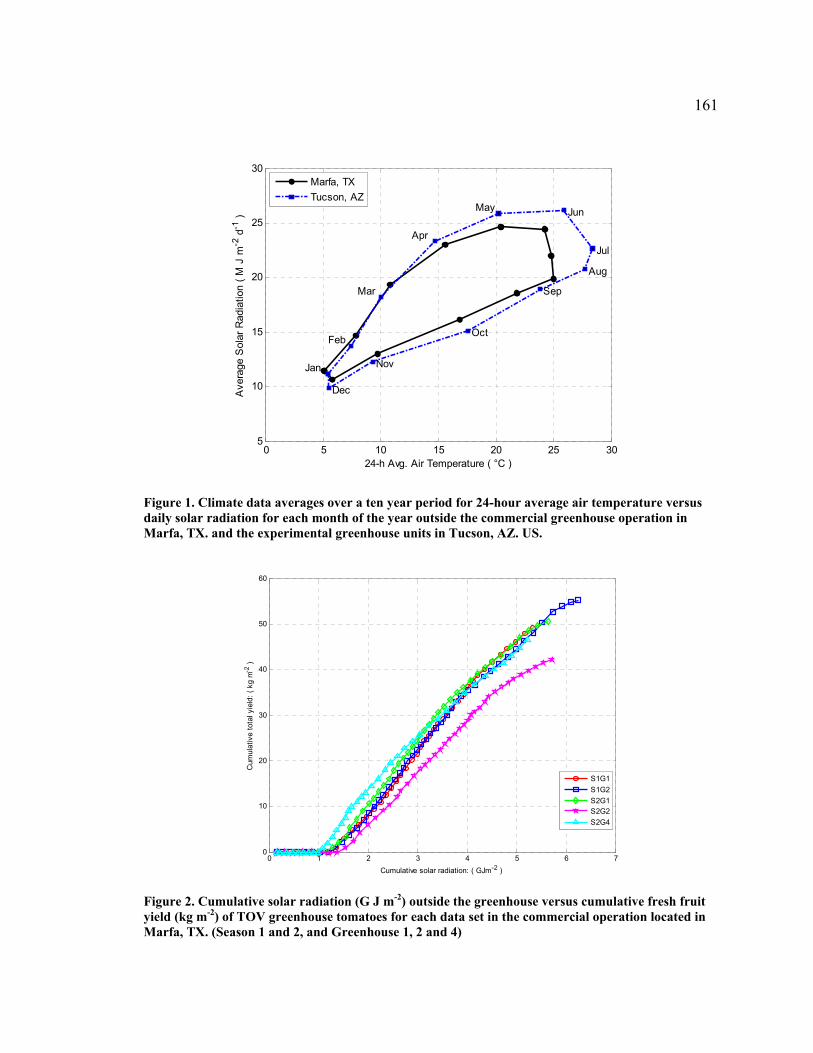
161
0 5 10 15 20 25 305
10
15
20
25
30
Jan
Feb
Mar
Apr
May Jun
Jul
Aug
Sep
Oct
Nov
Dec
24-h Avg. Air Temperature ( °C )
Ave
rage
Sol
ar R
adia
tion
( M J
m -2
d-1
)
Marfa, TXTucson, AZ
Figure 1. Climate data averages over a ten year period for 24-hour average air temperature versus daily solar radiation for each month of the year outside the commercial greenhouse operation in Marfa, TX. and the experimental greenhouse units in Tucson, AZ. US.
0 1 2 3 4 5 6 70
10
20
30
40
50
60
Cumulative solar radiation: ( GJm-2 )
Cum
ulat
ive
tota
l yie
ld: (
kg
m-2
)
S1G1S1G2S2G1S2G2S2G4
Figure 2. Cumulative solar radiation (G J m-2) outside the greenhouse versus cumulative fresh fruit yield (kg m-2) of TOV greenhouse tomatoes for each data set in the commercial operation located in Marfa, TX. (Season 1 and 2, and Greenhouse 1, 2 and 4)
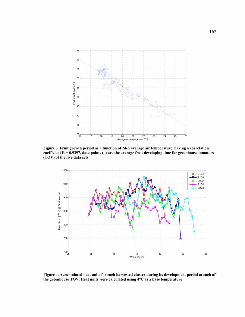
162
16 17 18 19 20 21 22 23 24 25 2630
35
40
45
50
55
60
65
70
75
Average air temperature ( °C )
Frui
t gro
wth
per
iod
( d )
Figure 3. Fruit growth period as a function of 24-h average air temperature, having a correlation coefficient R = 0.9397, data points (o) are the average fruit developing time for greenhouse tomatoes (TOV) of the five data sets
25 35 45 3 13 23 25700
750
800
850
900
950
1000
Week of year
Hea
t Uni
ts: [
o C d
] @ S
Hd
Inte
rval
S1G1S1G2S2G1S2G2S2G4
Figure 4. Accumulated heat units for each harvested cluster during its development period at each of the greenhouse TOV. Heat units were calculated using 4°C as a base temperature

163
Tapped Delay Line
Y
Output Hidden Layer 2
Hidden Layer 1
:
XR
:
:
X1
X2 X3 X4
X5
N1 N2 N3
:
:
NS2
:
NS1
N1 N2 N3
:
:
D1D2: Dd
Input Vector
Figure 5. Focused time-delay dynamic neural network architecture for modeling and predicting yield, fruit fresh weight, and fruit growth period of TOV greenhouse tomatoes
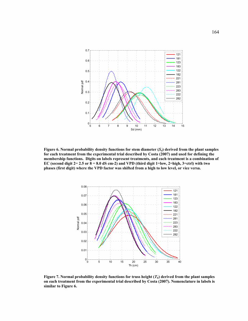
164
5 6 7 8 9 10 11 12 13 14 150
0.1
0.2
0.3
0.4
0.5
0.6
0.7
Sd (mm)
Nor
mal
121181123183122182221281223283222282
Figure 6. Normal probability density functions for stem diameter (Sd) derived from the plant samples for each treatment from the experimental trial described by Costa (2007) and used for defining the membership functions. Digits on labels represent treatments, and each treatment is a combination of EC (second digit 2= 2.5 or 8 = 8.0 dS cm-2) and VPD (third digit 1=low, 2=high, 3=ctrl) with two phases (first digit) where the VPD factor was shifted from a high to low level, or vice versa.
0 5 10 15 20 25 30 35 400
0.01
0.02
0.03
0.04
0.05
0.06
0.07
0.08
Th (cm)
Nor
mal
121181123183122182221281223283222282
Figure 7. Normal probability density functions for truss height (Th) derived from the plant samples on each treatment from the experimental trial described by Costa (2007). Nomenclature in labels is similar to Figure 6.
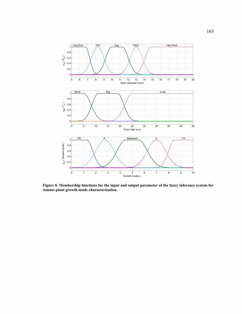
165
5 6 7 8 9 10 11 12 13 14 15 16 17 18 19 20
0
0.2
0.4
0.6
0.8
1
Stem diameter (mm)
μA (
Sd )
VeryThin Avg VeryThickThin Thick
0 5 10 15 20 25 30 35 40 45 50
0
0.2
0.4
0.6
0.8
1
Truss high (cm)
μB (
T h )
Short Avg Long
0 1 2 3 4 5 6 7 8 9 10
0
0.2
0.4
0.6
0.8
1
Growth mode(-)
μC
( G
row
th-m
ode
)
VR Balanced VVR V
Figure 8. Membership functions for the input and output parameter of the fuzzy inference system for tomato plant growth mode characterization.
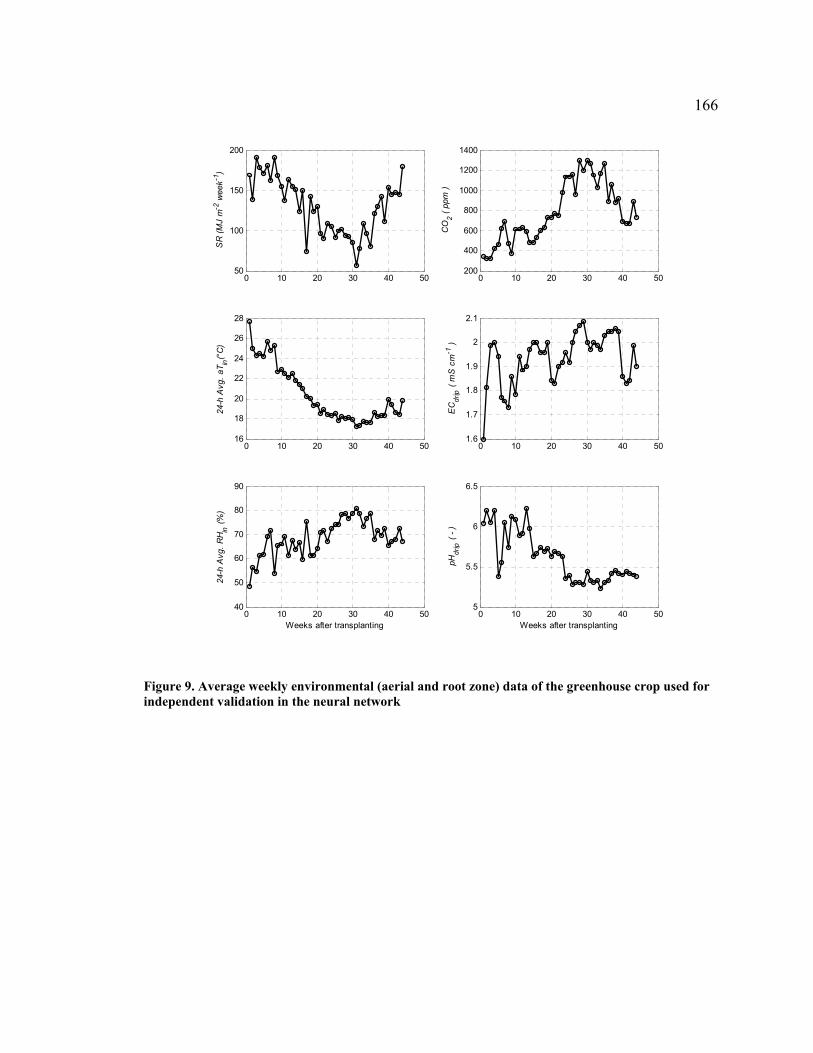
166
0 10 20 30 40 5050
100
150
200
SR
(MJ
m-2
wee
k-1)
0 10 20 30 40 5016
18
20
22
24
26
28
24-h
Avg
. aT in
(°C
)
0 10 20 30 40 5040
50
60
70
80
90
Weeks after transplanting
24-h
Avg
. RH in
(%)
0 10 20 30 40 50200
400
600
800
1000
1200
1400
CO
2 ( pp
m )
0 10 20 30 40 501.6
1.7
1.8
1.9
2
2.1
EC
drip
( m
S c
m-1
)
0 10 20 30 40 505
5.5
6
6.5
pH
drip
( - )
Weeks after transplanting
Figure 9. Average weekly environmental (aerial and root zone) data of the greenhouse crop used for independent validation in the neural network
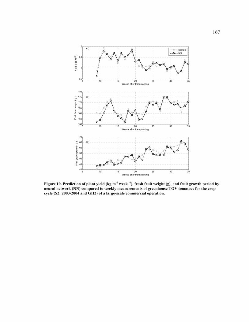
167
5 10 15 20 25 30 35150
155
160
165
170
175
180
Weeks after transplanting
Frui
t fre
sh w
eigh
t ( g
) B )
5 10 15 20 25 30 3540
45
50
55
60
65
70
Weeks after transplanting
Frui
t gro
wth
per
iod
( d ) C )
5 10 15 20 25 30 350.5
1
1.5
2
Weeks after transplanting
Yie
ld (
kg m
-2 )
A ) Sample
NN
Figure 10. Prediction of plant yield (kg m-2 week -1), fresh fruit weight (g), and fruit growth period by neural network (NN) compared to weekly measurements of greenhouse TOV tomatoes for the crop cycle (S2: 2003-2004 and GH2) of a large-scale commercial operation.

168
0 5 10 15 20 25 300
2
4
6
8
10
Weeks after Treatment
R
ep.<
---- B
alan
ced
---->
Veg
.
VPDLow VPDHigh A)
EC=2.5EC=8.0
0 5 10 15 20 25 300
2
4
6
8
10
Weeks after Treatment
R
ep.<
---- B
alan
ced
---->
Veg
.
VPDHigh VPDLow B)
0 5 10 15 20 25 300
2
4
6
8
10
Weeks after Treatment
R
ep.<
---- B
alan
ced
---->
Veg
.
VPDstd VPDstd C)
Figure 11. Growth-mode characterization of greenhouse beefsteak tomato plants during the production cycle for experimental trials inducing vegetative (Fig. A), reproductive (Fig. B) and balanced (Fig. C) growing conditions in Tucson, AZ for half of the experiment, then on WAT 16 the environment was switched to an opposite growth-mode.

169
0 10 20 30 400
2
4
6
8
10
R
ep.<
---- B
alan
ced
---->
Veg
.
Week After Transplanting
Season 1: 2002-2003
GH1)
0 10 20 30 400
2
4
6
8
10
Weeks after transplanting
R
ep.<
---- B
alan
ced
---->
Veg
. GH2)
0 10 20 30 400
2
4
6
8
10
Weeks after transplanting
R
ep.<
---- B
alan
ced
---->
Veg
.
Season 2: 2003-2004
GH1)
0 10 20 30 400
2
4
6
8
10
Weeks after transplanting
R
ep.<
---- B
alan
ced
---->
Veg
. GH2)
0 10 20 30 400
2
4
6
8
10
Weeks after transplanting
R
ep.<
---- B
alan
ced
---->
Veg
. GH4)
0 10 20 30 400
2
4
6
8
10
Weeks after transplanting
R
ep.<
---- B
alan
ced
---->
Veg
. GH3)
Figure 12. Growth-mode characterization of greenhouse tomato plant during the production cycle in a commercial operation in Marfa, TX.
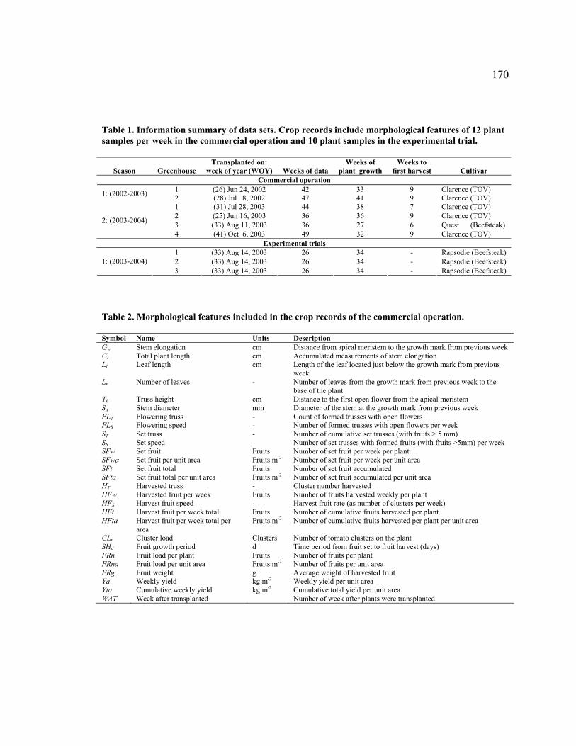
170
Table 1. Information summary of data sets. Crop records include morphological features of 12 plant samples per week in the commercial operation and 10 plant samples in the experimental trial.
Season
Greenhouse
Transplanted on: week of year (WOY)
Weeks of data
Weeks of plant growth
Weeks to first harvest
Cultivar
Commercial operation 1 (26) Jun 24, 2002 42 33 9 Clarence (TOV) 1: (2002-2003) 2 (28) Jul 8, 2002 47 41 9 Clarence (TOV) 1 (31) Jul 28, 2003 44 38 7 Clarence (TOV) 2 (25) Jun 16, 2003 36 36 9 Clarence (TOV) 3 (33) Aug 11, 2003 36 27 6 Quest (Beefsteak) 2: (2003-2004)
4 (41) Oct 6, 2003 49 32 9 Clarence (TOV) Experimental trials
1 (33) Aug 14, 2003 26 34 - Rapsodie (Beefsteak) 2 (33) Aug 14, 2003 26 34 - Rapsodie (Beefsteak) 1: (2003-2004) 3 (33) Aug 14, 2003 26 34 - Rapsodie (Beefsteak)
Table 2. Morphological features included in the crop records of the commercial operation.
Symbol Name Units Description Gw Stem elongation cm Distance from apical meristem to the growth mark from previous week Gt Total plant length cm Accumulated measurements of stem elongation Ll Leaf length cm Length of the leaf located just below the growth mark from previous
week Ln Number of leaves - Number of leaves from the growth mark from previous week to the
base of the plant Th Truss height cm Distance to the first open flower from the apical meristem Sd Stem diameter mm Diameter of the stem at the growth mark from previous week FLT Flowering truss - Count of formed trusses with open flowers FLS Flowering speed - Number of formed trusses with open flowers per week ST Set truss - Number of cumulative set trusses (with fruits > 5 mm) SS Set speed - Number of set trusses with formed fruits (with fruits >5mm) per week SFw Set fruit Fruits Number of set fruit per week per plant SFwa Set fruit per unit area Fruits m-2 Number of set fruit per week per unit area SFt Set fruit total Fruits Number of set fruit accumulated SFta Set fruit total per unit area Fruits m-2 Number of set fruit accumulated per unit area HT Harvested truss - Cluster number harvested HFw Harvested fruit per week Fruits Number of fruits harvested weekly per plant HFS Harvest fruit speed - Harvest fruit rate (as number of clusters per week) HFt Harvest fruit per week total Fruits Number of cumulative fruits harvested per plant HFta Harvest fruit per week total per
area Fruits m-2 Number of cumulative fruits harvested per plant per unit area
CLn Cluster load Clusters Number of tomato clusters on the plant SHd Fruit growth period d Time period from fruit set to fruit harvest (days) FRn Fruit load per plant Fruits Number of fruits per plant FRna Fruit load per unit area Fruits m-2 Number of fruits per unit area FRg Fruit weight g Average weight of harvested fruit Ya Weekly yield kg m-2 Weekly yield per unit area Yta Cumulative weekly yield kg m-2 Cumulative total yield per unit area WAT Week after transplanted Number of week after plants were transplanted
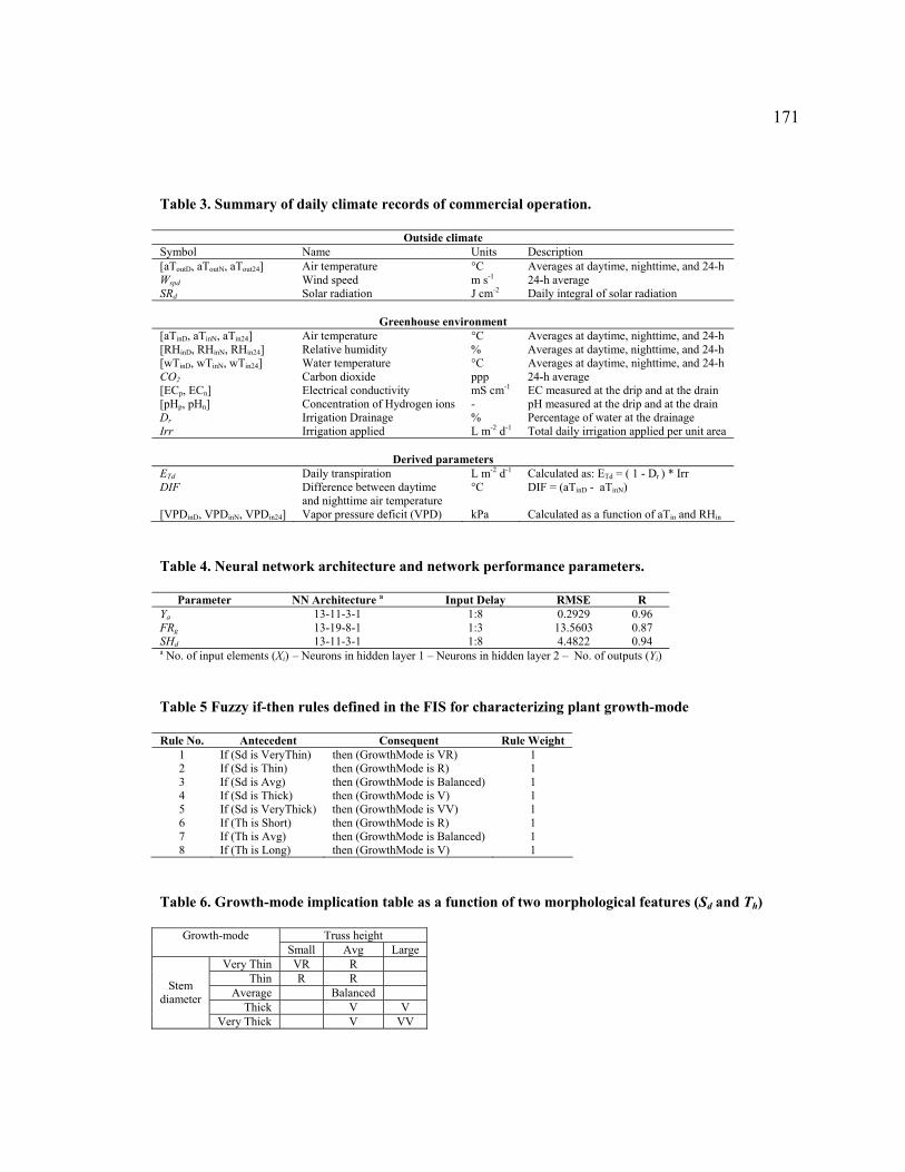
171
Table 3. Summary of daily climate records of commercial operation.
Outside climate Symbol Name Units Description [aToutD, aToutN, aTout24] Air temperature °C Averages at daytime, nighttime, and 24-h Wspd Wind speed m s-1 24-h average SRd Solar radiation J cm-2 Daily integral of solar radiation
Greenhouse environment
[aTinD, aTinN, aTin24] Air temperature °C Averages at daytime, nighttime, and 24-h [RHinD, RHinN, RHin24] Relative humidity % Averages at daytime, nighttime, and 24-h [wTinD, wTinN, wTin24] Water temperature °C Averages at daytime, nighttime, and 24-h CO2 Carbon dioxide ppp 24-h average [ECp, ECn] Electrical conductivity mS cm-1 EC measured at the drip and at the drain [pHp, pHn] Concentration of Hydrogen ions - pH measured at the drip and at the drain Dr Irrigation Drainage % Percentage of water at the drainage Irr Irrigation applied L m-2 d-1 Total daily irrigation applied per unit area
Derived parameters
ETd Daily transpiration L m-2 d-1 Calculated as: ETd = ( 1 - Dr ) * Irr DIF Difference between daytime
and nighttime air temperature °C DIF = (aTinD - aTinN)
[VPDinD, VPDinN, VPDin24] Vapor pressure deficit (VPD) kPa Calculated as a function of aTin and RHin
Table 4. Neural network architecture and network performance parameters.
Parameter NN Architecture a Input Delay RMSE R Ya 13-11-3-1 1:8 0.2929 0.96 FRg 13-19-8-1 1:3 13.5603 0.87 SHd 13-11-3-1 1:8 4.4822 0.94 a No. of input elements (Xi) – Neurons in hidden layer 1 – Neurons in hidden layer 2 – No. of outputs (Yi)
Table 5 Fuzzy if-then rules defined in the FIS for characterizing plant growth-mode
Rule No. Antecedent Consequent Rule Weight 1 If (Sd is VeryThin) then (GrowthMode is VR) 1 2 If (Sd is Thin) then (GrowthMode is R) 1 3 If (Sd is Avg) then (GrowthMode is Balanced) 1 4 If (Sd is Thick) then (GrowthMode is V) 1 5 If (Sd is VeryThick) then (GrowthMode is VV) 1 6 If (Th is Short) then (GrowthMode is R) 1 7 If (Th is Avg) then (GrowthMode is Balanced) 1 8 If (Th is Long) then (GrowthMode is V) 1
Table 6. Growth-mode implication table as a function of two morphological features (Sd and Th)
Truss height Growth-mode Small Avg Large
Very Thin VR R Thin R R
Average Balanced Thick V V
Stem diameter
Very Thick V VV