intelligence semi-automated wheelchair (obstacle …
TRANSCRIPT

INTELLIGENCE SEMI-AUTOMATED WHEELCHAIR
(OBSTACLE DETECTION SYSTEM)
LIEW YEE CHANG
A project report submitted in partial fulfilment of the
requirements for the award of Bachelor of Engineering
(Hons.) Mechatronics Engineering
Faculty of Engineering and Science
Universiti Tunku Abdul Rahman
May 2013

ii
DECLARATION
I hereby declare that this project report is based on my original work except for
citations and quotations which have been duly acknowledged. I also declare that it
has not been previously and concurrently submitted for any other degree or award at
UTAR or other institutions.
Signature : _________________________
Name : Liew Yee Chang
ID No. : 09UEB08350
Date : _________________________
iii
APPROVAL FOR SUBMISSION
I certify that this project report entitled “INTELLIGENCE SEMI-AUTOMATED
WHEELCHAIR (OBSTACLES DETECTION SYSTEM)” was prepared by
LIEW YEE CHANG has met the required standard for submission in partial
fulfilment of the requirements for the award of Bachelor of Engineering (Hons.)
Mechatronics Engineering at Universiti Tunku Abdul Rahman.
Approved by,
Signature : _________________________
Supervisor : Dr. LEONG WAI YIE
Date : _________________________

iv
The copyright of this report belongs to the author under the terms of the
copyright Act 1987 as qualified by Intellectual Property Policy of University Tunku
Abdul Rahman. Due acknowledgement shall always be made of the use of any
material contained in, or derived from, this report.
© 2013, LIEW YEE CHANG. All right reserved.
v
ACKNOWLEDGEMENTS
I would like to thank everyone who had contributed to the successful completion of
this project. I would like to express my gratitude to my research supervisor, Dr.
Leong Wai Yie for his invaluable advice, guidance and his enormous patience
throughout the development of the research. Besides that, I would like to thanks to
my lecturer, Mr Danny Ng Wee Kiat for giving me advice in term of hardware and
electronics design. At the same time, the lab officer, Mr Teoh Boon Yew always
provides good support in tooling and instrument.
In addition, I would also like to express my gratitude to my loving family for
giving me mentally support especially when I was under depression. Finally, I would
also thanks to my team members, Mr Fang Jin Yau, Mr Loh Jia Zhuan and Mr Ng
Ching Ruey for their contribution and team work.

vi
INTELLIGENCE SEMI-AUTOMATED WHEELCHAIR
(OBSTALES DETECTION SYSTEM)
ABSTRACT
An obstacle detection system that applies on an intelligence semi-automated
wheelchair was build. The system was specially built for patients who were slow in
response like patience with unsound mind or Parkinson. It was build to assist patients
in transportation so that they were more independent. The main purpose of this
system was to help the patient in preventing collision during travelling with
wheelchair. Therefore, this system will improve the safety factor. This project
focused in indoor use as it was design for the wheelchair used in hospital. Therefore,
situations in a hospital were more concern during the design process. Several
methods had been introduced for this type of system especially in smart mobile robot.
Method uses may affect by the sensor as there are several types of vision sensor with
different characteristics available in the market. Other similar projects were studied
to have a better understanding on the system before the system was design.
MaxSonar-EZ1 ultrasonic sensor from Cytron Technologies and PIC18F4520 from
MicroChip Technology were the hardware used in this project to build the obstacle
detection system. The surrounding information from the sensors were feed into the
microcontroller that having special algorithm for processing. Edge detection and wall
following concepts were used in the algorithm. After that, the microcontroller
provided the specific output to the driving system to react accordingly. Two modes,
semi-automated and automated were designed in the project for two control types.
Different tests were carried out for the system and the results were satisfied. The
system behaviour and reliability were discussed with the result. Finally, the system
was concluded that it was reliable to certain degree as it did behave according to
objectives. A recommendation section was included as the system was still able to
improve. Further study was needed to make the system perfect.

vii
TABLE OF CONTENTS
DECLARATION ii
APPROVAL FOR SUBMISSION iii
ACKNOWLEDGEMENTS v
ABSTRACT vi
TABLE OF CONTENTS vii
LIST OF TABLES x
LIST OF FIGURES xi
LIST OF SYMBOLS / ABBREVIATIONS xv
LIST OF APPENDICES xvi
CHAPTER
1 INTRODUCTION 1
1.1 Background 1
1.2 Aim and Objectives 2
1.3 Flow of Content 4
2 LITERATURE REVIEW 5
2.1 Introduction 5
2.2 Hardware 5
2.2.1 Introduction 5
2.2.2 Sensors 7
2.2.3 Microprocessor and DAQ 18
2.3 Software 24
2.3.1 Introduction 24

viii
2.3.2 MPLAB IDE 25
2.3.3 LabVIEW 26
2.4 Global and Local Planning 27
2.5 Concept and Algorithm 27
2.5.1 Introduction 27
2.5.2 Fuzzy Logic 28
2.5.3 Edge Detection 30
2.5.4 Wall-Following 32
2.5.5 Black Hole 34
2.5.6 Potential Field 34
2.5.7 Personal Concept 36
3 METHODOLOGY 38
3.1 Introduction 38
3.2 Ultrasonic Sensor 38
3.3 PIC Microcontroller 39
3.4 Mechanical Development 41
3.5 Electronics Development 41
3.6 Concept and Algorithm 42
4 RESULTS AND DISCUSSIONS 47
4.1 Mechanical Development 47
4.2 Study of Design’s Behaviour 51
4.3 Electronics Development 56
4.4 System Development 59
4.5 System Testing 63
4.5.1 Introduction 63
4.5.2 Semi-Automated Mode 64
4.5.3 Automated Mode 66
4.5.4 Discussion on System Test 69
4.6 Systems Combination 70
4.6.1 Introduction 70
4.6.2 Semi-Automated Mode 70

ix
4.6.3 Automated Mode 82
5 CONCLUSION AND RECOMMENDATIONS 88
5.1 Conclusion 88
5.2 Recommendations 88
REFERENCES 90
APPENDICES 92

x
LIST OF TABLES
TABLE TITLE PAGE
2.1 Characteristics of MaxSonar-EZ1 and HRLV-
MaxSonar-EZ 9
2.2 Characteristics of E3ZM-CT81 and E3Z LT86 14
2.3 Characteristics of Webcam C110 and FQ-
MS120-M 17
2.4 Sensors Comparison 17
2.5 Characteristics of NI DAQ Devices 23
2.6 Microcontroller and DAQ Comparison 24
4.1 Distance Measuring Test Result 52
4.2 Sensor Coverage Test Result 54
4.3 Percentage Error for Sensor Coverage Test
Result 55
4.4 Microcontroller Pin Assignment 62
4.5 Range Test Result 79
4.6 Range Test Result in Percentage 80
4.7 Random Moving Test Result 80
4.8 Automated System Test Result 83

xi
LIST OF FIGURES
FIGURE TITLE PAGE
2.1 Ultrasonic Sensors (MaxBotix, 2012) 7
2.2 Block diagram of the ultrasonic system (Mazo,
2001) 8
2.3 Beam Characteristics of HRLV-MaxSonar-EZ1
(MaxBotix, 2012) 9
2.4 Beam Characteristics of MaxSonar-EZ1
(Maxbotix, 2006) 10
2.5 Laser Sensors (OMRON, n.d.) 10
2.6 Object location: lightened scene (top) and
segmentation (bottom) (Mazo, 2001) 12
2.7 CAD drawing of active 3D triangulation laser
scanner integrated on the movable part of
Replicator robot (Fu et al, 2012) 13
2.8 Experiment result (Fu et al, 2012) 13
2.9 Vision Sensor (OMRON, n.d.) 14
2.10 Obstacle Avoidance Robot (Kinsky et al, 2011) 15
2.11 Experimental Result on Obstacles and Non-
obstacles (Kinsky et al, 2011) 16
2.12 Examples of PIC Microcontroller (Microchip
Technology Inc) 18
2.13 Harvard Architecture (Microchip Technology
Inc) 19
2.14 Examples of FPGA (Altera, 2006) 20

xii
2.15: Logic Cell in FPGA (Nicolle, J. P., 2006) 20
2.16 NI DAQmx 9.0.2 (National Instrument, 2012) 21
2.17 Data Sampling in ADC (National Instrument,
2012) 23
3.1 Position of Six MaxSonar-EZ1 Ultrasonic
Sensors 39
3.2 PIC18F4520 Pin Diagram (Microchip
Technology Inc, 2004) 40
3.3 Automated Mode 45
3.4 Semi-Automated Mode 46
4.1 Mechanical Design Version 1 47
4.2 Mechanical Design Version 2 48
4.3 Mechanical Design Version 3 with SolidWorks 49
4.4 Constructed Mechanical Design Version 3 49
4.5 Ultrasonic Sensor on Wheelchair 50
4.6 Ultrasonic Sensor Set 50
4.7 Distance Measuring Test Setting 51
4.8 Graph of Actual Distance vs Measured Distance 52
4.9 Graph of Percentage Error for Distance
Measuring Test 52
4.10 Sensor Coverage Test Setting 54
4.11 Mahjong Paper with Angles Setting 54
4.12 Graph of Percentage Error for Sensor
Coverage Test 56
4.13 Schematic and PCB Board of Obstacle
Detection System 58
4.14 Obstacle Detection System Board 58
4.15 Schematic and PCB Board of Power Board 58

xiii
4.16 Power Board 59
4.17 Ultrasonic Sensor Indicator 59
4.18 Combination between Electronics and
Mechanical 62
4.19 Testing Circuit on Breadboard 63
4.20 Testing Circuit Breadboard on Wheelchair 63
4.21 Front Sensor Test 65
4.22 Left Sensor Test 65
4.23 Right Sensor Test 65
4.24 Back Sensor Test 66
4.25 Multiple Sensors Test 66
4.26 Automated Test 1 68
4.27 Automated Test 2 68
4.28 Automated Test 3 68
4.29 Sensor Wave Interruption 70
4.30 Four Obstacles for Testing 74
4.31 Contact Tachometer 74
4.3 Determined rpm with Contact Tachometer 74
4.33 Full Speed Test with PC Box Obstacle 75
4.34 Random Moving Test Setting 75
4.35 Obstacle Detection with Forward Motion 78
4.36 Obstacle Detection with Right Turning Motion 79
4.37 Chance to Escape from Trap 79
4.38 Graph of Random Moving Test 81
4.39 Automated System Test 83
4.40 Graph of Automated System Test 84

xiv
4.41 Previous Automated Mode Flow Chart 86

xv
LIST OF SYMBOLS / ABBREVIATIONS
v speed of wheelchair, m/s
r radius of tachometer wheel, m
rpm number of revolution per minute, rpm
Vref voltage reference, V
TAD A/D conversion clock, s
Fosc oscillator clock frequency, Hz
TACQ acquisition time, s
s distance, m
u initial velocity, m/s = 0m/s
t time taken, s
a acceleration, m/s2

xvi
LIST OF APPENDICES
APPENDIX TITLE PAGE
A Coding 92
B Turnitin Report 101
C Time Schedule 104
D Gantt Chart 106
1
CHAPTER 1
1 INTRODUCTION
1.1 Background
Due to the advance in technology, autonomous had become a popular research topic
nowadays. Intelligent mobile robot like Honda ASIMO no longer odd to people and
more and more mobile robot with different application had been introduced. Under
medical field, wheelchair had been transform from a traditional wheelchair into an
autonomous wheelchair as well.
Wheelchair was first introduced in 1595 where the Spanish King, Philip II of
Spain who sat on a chair with small wheels mounted at the end of each leg. However,
the chair cannot be self-propelled and need a servant to push it. In 1881, larger
wheels are used and rim was added on each wheel for self-propelled purpose.
Furthermore, due to the need of man power, wheelchair again transformed into
motorized wheelchair in 1916 where user are able to control the movement with only
a controller like joystick. This kind of wheelchair is quite widely use nowadays, but
it is still insufficient when it came to patients who cannot control the wheelchair
properly with the joystick.
Patients with slow in response, unsound mind, Parkinson’s and so on is
having difficulty in controlling the motorized wheelchair with the controller.
Therefore, another advanced transformation is needed on the motorized wheelchair
to form an autonomous wheelchair. An autonomous wheelchair shall include extra
2
features like navigation system, obstacles detection system, auto-adjustable seat with
pre-set program, automatic speed control and so on. This wheelchair shall have the
ability to assist the patient or automatically transport the patient from a destination to
another destination safely.
Lots of study and research had to be gone through in order to come out with
an autonomous wheelchair. Some researches in intelligent mobile robot can be used
as a reference because it also has the similar features such as the obstacle detection.
Intelligent mobile robot with navigation system is usually come with an obstacle
detection feature to form a complete system. It is a huge study in obstacle detection
system as there are a lot of phenomena to be concerned. Therefore, this paper is
focusing and discuss on the obstacle detection system for the Intelligence Semi-
Automated Wheelchair.
Research on the obstacle detection system is not a new topic especially in
mobile robot. With obstacle detection system, a mobile robot is assumed to be
intelligent to a certain degree as it can transport without hitting an obstacle (Yi et al,
2009). With the development of sensor technologies, different types of obstacle
detection system had been introduced. Since human being is using vision to detect an
obstacle, vision sensor like ultrasonic sensor, camera, infrared sensor, or laser sensor
is used to build an obstacle detection system. Besides hardware, software also plays
an important role that work as the brain in the system. For example, neuron network
to allow the system to learn with samples and fuzzy logic control to control the
output (wheel) with a series of fuzzy control rule based on the input (sensor) given.
1.2 Aim and Objectives
The aim of this paper is to study on the obstacle detection system in term of the
hardware as well as the software. This system is going to combine with other features
like driving system and navigation system to form the Intelligence Semi-Automated
Wheelchair. The main purpose of this obstacle detection system is to detect obstacle,

3
identify the location of obstacle, and provide the right outputs to the driving system
to response accordingly. It must help the patient who is slow in response to detect
obstacle and prevent collision from happen. Safety of the user is the main concern in
this study as obstacle detection system provides the safety feature to the wheelchair
design. These abilities help the Intelligence Semi-Automated Wheelchair deal with
the unknown environment especially under the indoor environment which is full with
unexpected activities and limited space.
As mention previously, this system is going to combine with the driving
system and navigation system. The Intelligence Semi-Automated Wheelchair is
designed especially for hospital use where there will be a special track build for the
navigation system. During the automatic mode where the autonomous wheelchair is
running by itself, it will follow the track to travel from a destination to another
destination. Therefore, the main obstacle to be concerned by the obstacle detection
system is the obstacle that lies on the track. For examples, in a hospital, water bottle,
medicine box and trolley might be accidently left on the walkway and blocking the
wheelchair path. Besides static obstacles, moving object like human and moving
trolley might also happen to be blocking the wheelchair path in a short period.
Therefore, the obstacle detection system not just to obey the obstacle detection
feature but also has to be respond in time to overcome the emergency situation with
the moving obstacles.
Besides automated, the obstacle detection system also include semi-
automated mode. This mode is activated when the user is controlling the wheelchair
motion. The motion is decided by the user and the obstacle detection system works
as the supporter. The system limits the particular motion when it detects an obstacle
blocking the way. For example, it limits the forward motion from the user when there
are obstacles in front of the wheelchair. Therefore, the main objective of this mode is
to help the user in detecting the obstacles and preventing the user from controlling
the wheelchair move toward the obstacles.
As a conclusion, the objectives of the obstacle detection system in this project
are:
4
detect static obstacles like transparent water bottle, medicine box, chair and
table and then preventing collision
detect moving obstacle detection like kids and moving trolley and then
respond in time to avoid collision
detect obstacles that blocking the wheelchair path and then avoid it to
continue the movement (automated mode)
detect obstacles that present at the wheelchair surrounding and then limit
particular motion from user control (semi-automated mode)
communicate well with driving system to have an efficient and reliable
system
the algorithm shall provide a smooth travelling to maintain the user
comfortable
1.3 Flow of Content
The content of this paper is following the flow which starts with literature review
where other related researches were studied base on this paper. Research
methodology, the concepts or methods used in this paper, follow with the results and
discussions that present the outcome of this study and the analysis of the outcome.
Final part will be the conclusion and recommendations where a final conclusion base
on the whole research is presented and further improvement for the research is stated.

5
CHAPTER 2
2 LITERATURE REVIEW
2.1 Introduction
This section is going to discuss about the study of other research articles or reports
that related to this paper. It is divided into few subsections to discuss separately, so
that the paper is more organized and easy to be read. A final subsection is included in
each group of hardware to have a comparison between the components. The
comparison is done among the hardware instead of software because the choice of
software used is most likely depending on the hardware used. For example, MPLAB
was designed especially for supporting PIC microcontroller. The comparison is done
in table form which provides a better view for the author to choose the best and most
suitable component in this project. Besides that, concepts and algorithms used by the
researches were also being studied and discussed.
2.2 Hardware
2.2.1 Introduction
Hardware used in obstacles detection system is one of the important aspects that
should be paid more attention. Obstacles detection system is strongly rely on the
vision sensor used to get the information from the surrounding environment as the
input data for the system. There are many types of sensor available nowadays where

6
each of it is having their own characteristics that suits different conditions. The
mainly used sensors to avoid obstacles are ultrasonic sensors, vision sensors, infrared
sensors, laser sensors and proximity sensors (Yang et al, 2010). Some of the sensors
were studied and discussed based on their characteristics. There are a few companies
in Malaysia which producing electronics components. Therefore, the characteristics
of the sensors are taken from the datasheet provided to do the comparison.
Sensor itself is not enough to produce an intelligence system; a “brain” is
needed to process the input from the sensor and provides the intelligence decision.
The “brain” mentioned here will be the processor or commonly known as the
microprocessor in mobile robot field. Unfortunately, a microprocessor may not be
powerful enough to support a heavy processing. A computer processor is another
choice when come into handling a heavy processing task. This situation is common
when come to image processing. Due to the limited input ports of a computer, a data
transmitting body is needed to link between the sensors and computer for
communication purpose. The data transmitting body usually called as data
acquisition system (DAS or DAQ). Instead of microprocessor, microcontroller will
be a better choice because microcontroller is a microprocessor with extra features
like PWM. Besides that, it is also not rare to use a programmable logic device like
field-programmable gate array (FPGA) for fast signal processing (Gojić et al, 2011).
Therefore, PIC microcontroller, FPGA and NI DAQ board were studied and
discussed in this section.

7
2.2.2 Sensors
2.2.2.1 Ultrasonic Sensor
Figure 2.1: Ultrasonic Sensors (MaxBotix, 2012)
Figure 2.1 shows the examples of ultrasonic sensor. It is very clear that ultrasonic
sensor uses ultrasound to detect an obstacle. This kind of sensor is very common in
obstacles detection system as it is low in cost with mature technology and generates
simple range data. The location of the obstacle can be detected by the ultrasonic
distance that using the time difference. This can be explained through the working
principle of an ultrasonic sensor.
Ultrasonic sensor consists of a transmitter and a receiver. First, ultrasonic
transmitter launches ultrasonic wave in a direction which then spreads in the air. At
the same time of the wave launches, the sensor begins timing. When the ultrasonic
wave encounter an obstacle that blocking it from transmitting further, the wave will
immediately reflect back to the sensor and receive by the sensor receiver. The timing
will stop if the receiver receives a signal. In this way, it can calculate the distance of
obstacles from the launcher according to the velocity of the ultrasonic wave and the
time interval recorded by the sensor timer (Yi et al, 2009).
The disadvantage of ultrasonic sensor will be the poor direction and limited
angle ranging which caused single channel of ultrasonic ranging system insufficient
to meet the requirement of an obstacle detection system. Blind spots tend to occur
due to this disadvantage. In order to overcome this problem, a lot of researches
include multiple sensors in their design and compensated the readings to produce a
better and more accurate outcome. Usually, they combined a number of ultrasonic
sensors in a ring-shape distribution to form a module and then mounted a few sets of
8
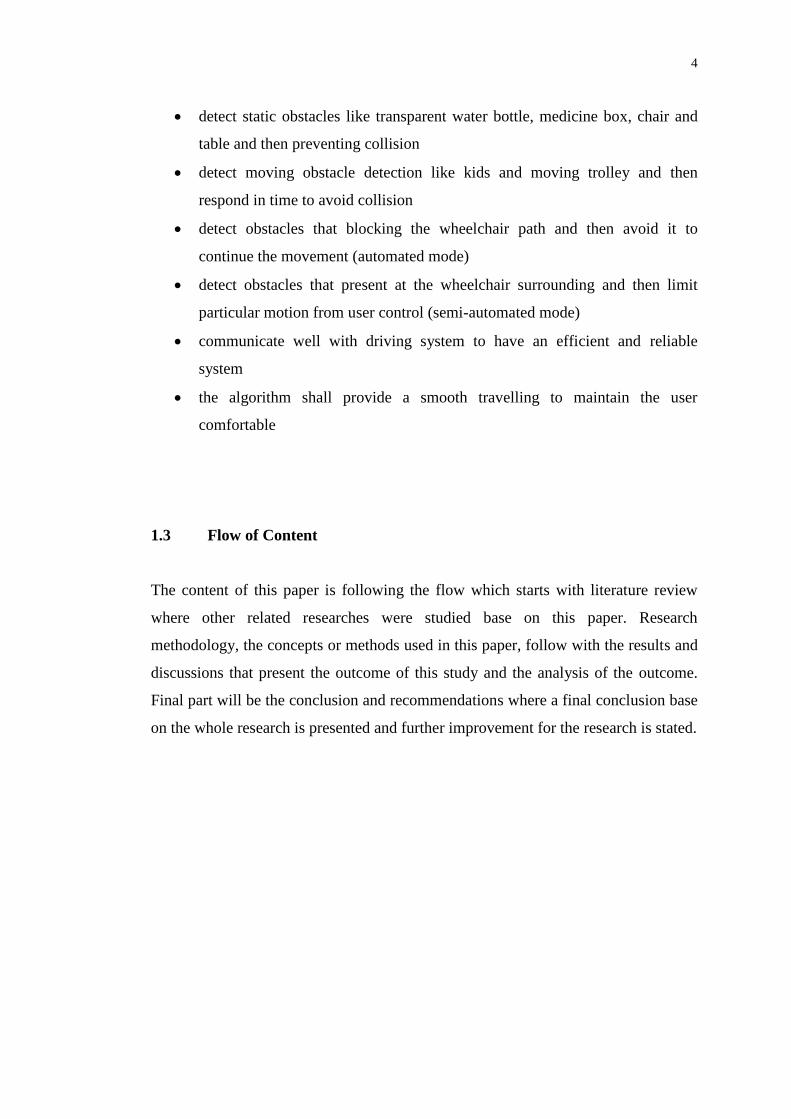
the module around the wheelchair. Figure 2.2 below shows the block diagram of the
ultrasonic system by Mazo 2001. In the figure, eight ultrasonic transducers were
combined to form a module and then four modules were mounted at each corner of
the wheelchair. It was clearly shows how the propagation of the ultrasonic wave had
covered the surrounding of the wheelchair. This was then overcome the blind spot
problem.
Figure 2.2: Block diagram of the ultrasonic system (Mazo, 2001)
There are two types of ultrasonic sensors produce by Cytron Technologies
Sdn Bhd that suited to be used in the obstacle detection system. Both of the sensors
can be refered to Figure 2.1 where the sensor on the left is MaxSonar-EZ1, and on
the right is a new model, HRLV-MaxSonar-EZ. The characteristic of both sensors
are taken from the datasheets provided by Cytron and presented in Table 2.1. Next,
the beam characteristics for both HRLV-MaxSonar-EZ and MaxSonar-EZ1 were
also studied and shown in Figure 2.3 and Figure 2.4 respectively.

9
Table 2.1: Characteristics of MaxSonar-EZ1 and HRLV-MaxSonar-EZ
Characteristic Ultrasonic Sensor
MaxSonar-EZ1 HRLV-MaxSonar-EZ
Range Detect Object: 0 – 254 in (6.45 m)
Sonar range: 6 – 254 in (0.15 – 6.45 m)
Detect Object: 1 mm – 5 m
Sonar range: 30 cm – 1 m
Supply
Voltage and
Current
Draw
5V supply with 2mA typical current
draw
2.5V to 5.5V supply with
nominal current draw of 2.5mA
to 3.1mA
Resolution 1 in (25.4 mm) 1 mm
Reading Rate 20 Hz (0.05 s) 10 Hz (0.1 s)
Outputs Serial (RS232)
Analog (10 mV/inch) (0.39 mV/mm)
Pulse width (147 uS/inch) (5.74
uS/mm)
Serial (RS232 or TTL)
Analog (0.92 mV/mm)
Pulse width (1 uS/mm)
Cost RM 138.00 RM 159.00
Figure 2.3: Beam Characteristics of HRLV-MaxSonar-EZ1 (MaxBotix, 2012)

10
Figure 2.4: Beam Characteristics of MaxSonar-EZ1 (Maxbotix, 2006)
2.2.2.2 Laser Sensor
Figure 2.5: Laser Sensors (OMRON, n.d.)

11
According to Fu et al, 2012, laser sensor could be categorized into time-of-flight
(TOF) and triangulation as shown in Figure 2.5 where TOF laser sensor emits a
straight line beam while triangulation laser sensor emits a triangular shape beam. The
TOF laser scanner has the advantages of a wide measuring range and high relative
accuracy at a long distance. In general application it can be considered as the ideal
straight line sensor to get the exact position of obstacle. Although TOF laser scanner
is having very high accuracy among the others, but it is very expensive and high
power consumption, so it is not practical to apply on an autonomous wheelchair that
makes the product unaffordable. Besides, the power source of a wheelchair is only
from the battery, so it is impossible to support a TOF laser sensor. On the other hand,
laser beam is harmful to human eyes. This is one of the factor causing laser scanner
is not widely used in mobile robot as it is moving around and may accidently emits
the laser beam on a human eye.
Comparing with TOF, triangulation laser sensor had a better advantage for
obstacle detection system. TOF emits only one narrow straight beam which only
detecting one point, while triangulation laser sensor had the ability to scan multiple
points simultaneously. This ability increases the scanning speed and yet improves the
system response. Besides that, triangulation laser sensor also lower in cost as well as
lower in power consumption as compare to TOF laser sensor. Due to these features,
triangulation laser sensor is more common used in mobile robot in detecting
obstacles as compare to TOF laser sensor. Laser sensor is used commonly to extract
the feature (obstacle) in 3D instead of 2D to have better information for advance
usage such as path selection.
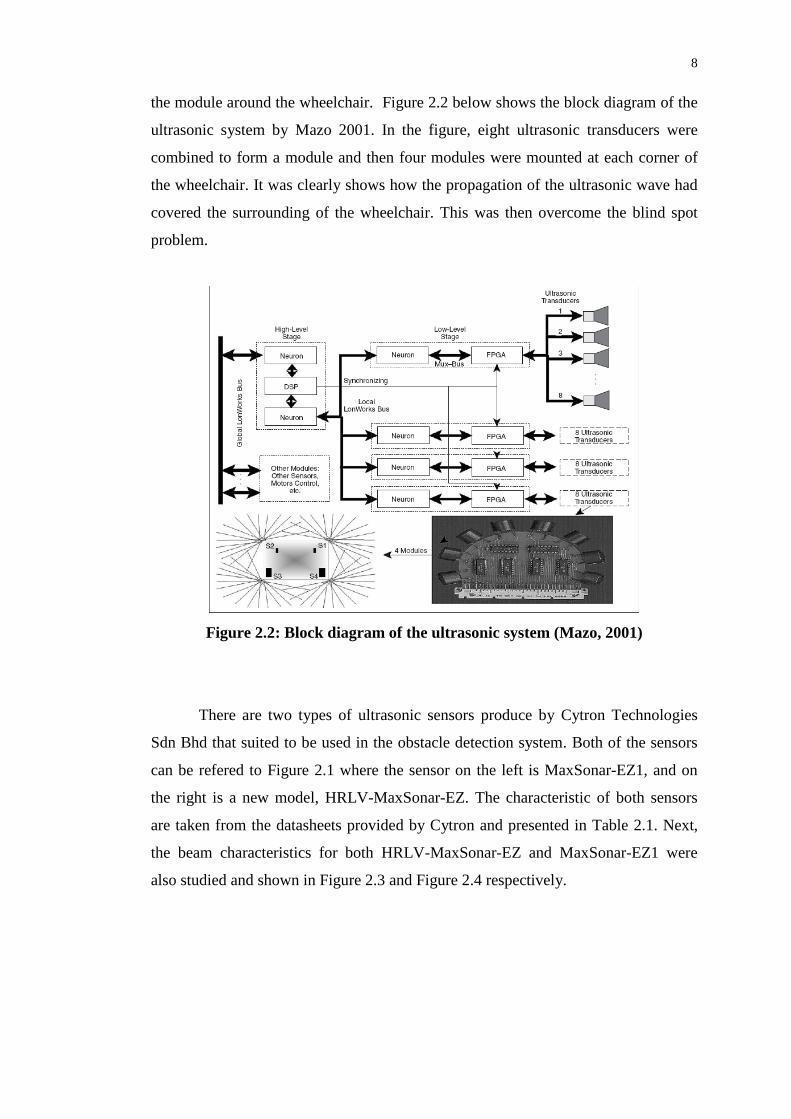
Refer to research by Mazo 2001, it used laser emitter and CCD camera to
detect obstacles in 3-D position of multiple points and space limits of the
environment. The laser beam was used to provide the position of the obstacles before
an image was captured by CCD camera. This made the segmentation process easier
and faster as the position of obstacle was determine clearly with red beam line in the
image as shown in Figure 2.6. After image processing, the result is shown in the
bottom image of Figure 2.6 where the whole image left only the beam lines for
further calculation.
12
Figure 2.6: Object location: lightened scene (top) and segmentation (bottom)
(Mazo, 2001)
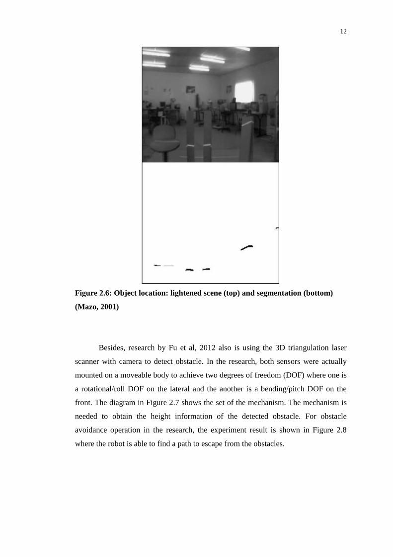
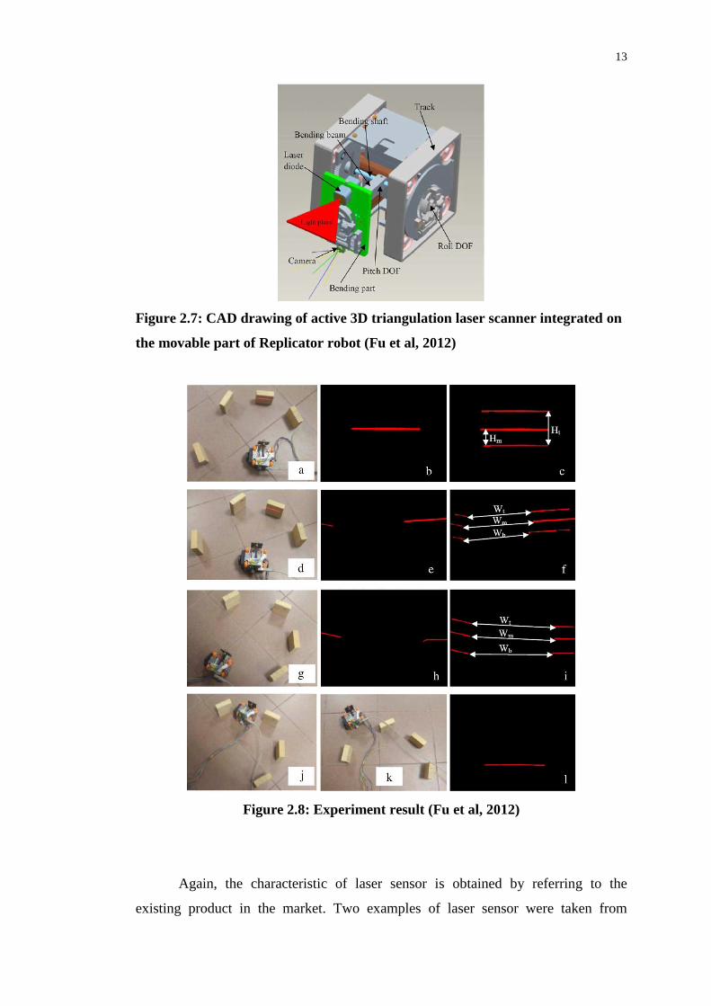
Besides, research by Fu et al, 2012 also is using the 3D triangulation laser
scanner with camera to detect obstacle. In the research, both sensors were actually
mounted on a moveable body to achieve two degrees of freedom (DOF) where one is
a rotational/roll DOF on the lateral and the another is a bending/pitch DOF on the
front. The diagram in Figure 2.7 shows the set of the mechanism. The mechanism is
needed to obtain the height information of the detected obstacle. For obstacle
avoidance operation in the research, the experiment result is shown in Figure 2.8
where the robot is able to find a path to escape from the obstacles.
13
Figure 2.7: CAD drawing of active 3D triangulation laser scanner integrated on
the movable part of Replicator robot (Fu et al, 2012)
Figure 2.8: Experiment result (Fu et al, 2012)
Again, the characteristic of laser sensor is obtained by referring to the
existing product in the market. Two examples of laser sensor were taken from

14
OMRON Industrial Automation, E3ZM-CT81 and E3Z LT86. The characteristics of
both products were extracted from the datasheet and presented in Table 2.2 below.
Table 2.2: Characteristics of E3ZM-CT81 and E3Z LT86
Characteristic Laser Sensor
E3ZM-CT81 E3Z LT86
Range 15 m 60 m
Standard Sensing
Object Opaque: 12 mm dia. min. Opaque: 12 mm dia. Min.
Minimum Detectable
Object (Typical)
6 mm dia. Opaque object at
3 m -
Supply Voltage 10 – 24 VDC 10 – 30 VDC
Current
Consumption
40 mA 35 mA
Response Time Operate or Reset: 1 ms max. Operate or Reset: 1 ms max.
2.2.2.3 Vision Sensor
Figure 2.9: Vision Sensor (OMRON, n.d.)
A vision sensor shows in Figure 2.9 actually is a camera that can be used as an
obstacle detection device. Vision sensor is the sensor which is having the most
similar vision as human being eye, stereo vision. The main advantage of vision
sensor on obstacles detection is the wide range detection ability which it can capture
an image and detect the whole obstacle or even multiple obstacles instead of just
detecting only one point on the obstacle. With this ability, it is able collect more

15
information such as the shape of an object and the speed of a moving object. With
multiple cameras or image sequences of a camera, the distance of the obstacle
detected from the sensor could be determined and the speed detection has also
become one of the ability of vision sensor.
Refer to the report from Kinsky et al, 2011, webcam which also consider as
one of the vision sensors was used in their project. Two webcams were mounted on
top of the obstacle avoidance robot to form the stereo vision as shown in Figure 2.10.
Figure 2.10: Obstacle Avoidance Robot (Kinsky et al, 2011)
With two sensors mounted, there will always be two images of the same
scene taken from different perspectives as shown in the example given in Figure 2.11.
Therefore, few processes had to pass through to form a single image before it could
proceed with the obstacle detection process. From the article, the experimental
results on real time are shown in Figure 2.11 where obstacles are present in white
boxes.

16
Figure 2.11: Experimental Result on Obstacles and Non-obstacles (Kinsky et al,
2011)
Since vision sensor grab image that consists of much information, image
processing is needed to handle all the information. This is the disadvantage of vision
sensor where time is needed to process the image before the system is able to
determine an obstacle. Lots of image processing like image smoothing, noise
filtering, edge enhancement and feature extraction needed a large calculation which
is also need much demanding on the central processor. This sensor considered bad in
real time situation as it is not able to provide fast response as needed in obstacle
detection system. Besides, this kind of sensor is highly affected by light intensity of
the surrounding, so it is not a very stable system when it comes to a different lighting
level environment. Next, it is also unable to detect obstacles that are transparent like
glass which may occurred in an unknown environment especially in hospital.
There are many types of vision sensor available in the market where
commercial type can be found in our daily life like webcam, while some of them are
from industrial sector. Therefore, two examples are taken from each fields and the
characteristic is presented in Table 2.3. The webcam example is from Logitech,
Webcam C110, while vision sensor from industrial field is FQ-MS120-M vision
sensor from OMRON.
17
Table 2.3: Characteristics of Webcam C110 and FQ-MS120-M
Characteristic Vision Sensor
Webcam C110 FQ-MS120-M
Optical Resolution True 640x480,
Interpolated 1.3MP -
Frame Rate 30 fps 60 fps (16.7 ms)
Focal Length 2.3 mm -
Supply Voltage - 21.6 – 26.4 VDC
Current
Consumption -
450mA max. (With FL-series
Strobe controller and lighting)
250mA max. (Without external
lighting)
Response Time Operate or Reset: 1 ms
max.
Operate or Reset: 1 ms max.
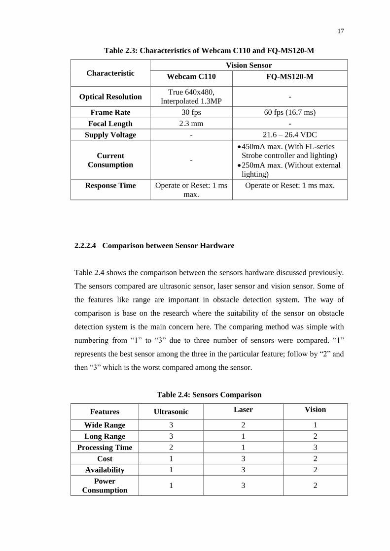
2.2.2.4 Comparison between Sensor Hardware
Table 2.4 shows the comparison between the sensors hardware discussed previously.
The sensors compared are ultrasonic sensor, laser sensor and vision sensor. Some of
the features like range are important in obstacle detection system. The way of
comparison is base on the research where the suitability of the sensor on obstacle
detection system is the main concern here. The comparing method was simple with
numbering from “1” to “3” due to three number of sensors were compared. “1”
represents the best sensor among the three in the particular feature; follow by “2” and
then “3” which is the worst compared among the sensor.
Table 2.4: Sensors Comparison
Features Ultrasonic Laser Vision
Wide Range 3 2 1
Long Range 3 1 2
Processing Time 2 1 3
Cost 1 3 2
Availability 1 3 2
Power
Consumption 1 3 2

18
The comparison shows that ultrasonic sensor is the best in term of non-
technical feature, while laser sensor is the best in term of technical feature. Vision
sensor is in the middle range among all three, but it is having a big problem with the
processing time. The time taken for processing is not suitable for real time
application like obstacle detection system where immediate response is needed as the
wheelchair is moving.
2.2.3 Microprocessor and DAQ
2.2.3.1 PIC Microcontroller
Figure 2.12: Examples of PIC Microcontroller (Microchip Technology Inc)
Figure 2.12 shows two example of PIC Microcontroller taken from MICROCHIP.
Due to the characteristics of PIC Microcontroller where low cost, low power
consumption, large user base, easy to use and easy to obtain, PIC Microcontrollers
are very popular among robot field. A PIC Microcontroller can be interpreted as a
mini computer where it has build in memory and RAM. In more details, PIC
Microcontroller has a central processing unit (CPU) to run the programs, random-
access memory (RAM) to hold variables, read-only memory (ROM) and input-output
line (I/O ports). As stated previously, PIC Microcontroller also includes extra built-in
peripheral like PWM, A/D and D/A converter (Premadi et al, 2009). PIC
Microcontroller can be programmed according to different application with all this
features. Unfortunately, the little PIC Microcontroller is unable to support huge
amount of programs like computer. It is useful in running a program and repeating

19
the program which is suitable to be used in robot field. Besides, it is less power
consumption that can support with only battery as carry by mobile robot.
PIC Microcontroller consider as the simplest processor where it consists low
number of instruction from about 35 instructions for the low-end PIC
Microcontroller to over 80 instructions for the high-end PIC Microcontroller. PIC
Microcontroller is using modified Harvard architecture (Figure 2.13) which
instructions and data come from separate sources. The architecture had simplified the
timing and microcircuit design greatly, which then improve the clock speed, reduce
the price and power consumption.
Figure 2.13: Harvard Architecture (Microchip Technology Inc)
MICROCHIP does provide some software like MPLAB, emulator and
compiler that support the PIC Microcontroller. With all this support tools, we can
write a program in some programming language like C language, compile the
language and burn into the PIC Microcontroller with the help of computer and
programmer device. The software also can be used in debugging mode to debug the
program before it is programmed into the microcontroller.

20
2.2.3.2 Field-Programmable Gate Array (FPGA)
Figure 2.14: Examples of FPGA (Altera, 2006)
As shown in Figure 2.14, FPGA is not just a single chip like PIC microcontroller but
it is actually an electronic board that consists of a lot of components. FPGA stands
for field-programmable gate array which is an integrated circuit designed with the
ability to be configured again by user after. This is why FPGA says to be “field-
programmable” that make it different from an application-specific integrated circuit
(ASIC). ASIC is customized for a particular use, while FPGA is manufactured for
general-purpose use. The FPGA configuration is generally specified using a
hardware description language (HDL).
FPGA contain many programmable logic components that call as logic cell.
Figure 2.15 shows the logic cell schematic that consists of a lookup table (LUT), a
D-flip flop and a 2-to-1 multiplexer. A logic cell can implement into any type of
logic function like AND or OR. All the logic cells in the FGPA can connect together
with the interconnect resources which are wires or multiplexes that placed around the
logic-cells. With this interconnect resources, different types of logic function can be
combined to create a complex logic function that useful in their corresponding
application. Therefore, FPGA is a good device to design digital logic application.
Figure 2.15: Logic Cell in FPGA (Nicolle, J. P., 2006)

21
Besides logic cell, FPGA also contains I/O cells where interconnect wires
will connect the cells to the boundary of FGPA. The function of this I/O cells is
similar to the I/O ports in PIC microcontroller that used to communicate with other
external element like sensor. FPGA is famous to be used in application where fast
speed process is needed. It is different from PIC microprocessor as it can run the
instructions in parallel. Multiple set of instruction can be run simultaneously with
FPGA as the cells can be separated and grouped accordingly.
As stated previously, hardware description language (HDL) is used in FPGA.
On other hand, a simple program structure can use schematic design to configure the
FPGA as it provides a clear visualization on the design. A common HDL uses
nowadays will be Verilog. Similar to microcontroller, FGPA companies also provide
their own software that supports their products. The software can be used to
complete the task like design entry, simulation, synthesis and place-and-route and
programming through special cable (JTAG). There are two main companies which
are Xilinx and Altera that controlling the FPGA market. Xilinx provides software
called ISE WebPack, while Altera provides Quartus II Web Edition. The software
will be further discussed in Software section.
2.2.3.3 DAQ Device
Figure 2.16: NI DAQmx 9.0.2 (National Instrument, 2012)

22
It is common that physical phenomenons around us like temperature, light and sound
provide us continuous signal which is called as analog signal. Unfortunately, analog
signal is not understandable by computer that use in processing the data. This is why
a data acquisition system is needed to sample the analog signals with a time of period
and convert the resulting samples into digital numeric values. Figure 2.16 shows an
example of DAQ device produced by National Instruments (NI). Data acquisition
system consists of three parts which are sensor, DAQ hardware and computer. DAQ
hardware will be the focus in this section.
DAQ hardware acts as the interface between a computer and signals from the
sensor that obtain from the measurement on the physical phenomenon on outside
world. It digitizes the analog signals into digital signals so that a computer can
interpret the data and use in processing. The three main components of DAQ
hardware are the signal conditioning circuitry, analog-to-digital converter (ADC),
and computer bus.
Signal conditioning circuitry is needed because the signal direct from sensor
may not powerful enough to be read or too powerful that may cause damage to the
electronic component. The signal from sensor has to be manipulated in order to suit
the requirement of the ADC component. This signal conditioning circuitry may
include amplification, attenuation, filtering, and isolation. Next, the analog signal
after signal conditioning stage will feed into ADC to be converted into digital signal.
Since analog signal vary continuously, it is impossible to sample the signal all the
time. ADC will sample an analog signal at a specific time and represent it in digital
form. One sample will take in every each time interval and from a digital signal as
shown in Figure 2.17.
From Figure 2.17, graph a) is the analog signal; follow by b) where each
signal value at each time interval is taken. Then, graph c) shows how to connect to
all reading to from a digital signal. Finally, graph d) shows the original signal is
reconstructed back from the digital signal by software. The digital signal will then
input into a computer with a computer bus. The computer bus serves as the
communication interface between the DAQ device and computer for passing
instructions and measured data. The examples of computer bus are USB, PCI, PCI

23
Express, Ethernet or even Wi-Fi. It is important when choosing the computer bus
because different type of bus suit different application condition.
Figure 2.17: Data Sampling in ADC (National Instrument, 2012)
Other than that, functions like digital-to-analog converter (DAC) to output
analog signals, digital I/O lines to input and output digital signals, and counter/timers
to count and generate digital pulses are also include in most of the DAQ hardware
nowadays. National Instruments is quiet popular with its DAQ device, so the
characteristic of NI DAQ device is study and shown in Table 2.5.
Table 2.5: Characteristics of NI DAQ Devices
Features Single Device
Portable DAQ Desktop DAQ
Bus USB, Wi-Fi, Ethernet PCI, PCI Express
Portability Best Good
Number of I/O Channels 1 – 100 1 – 100
I/O Configuration Fixed Fixed
Max Sample Rate 2 MS/s 10 MS/s
Built-In Signal Conditioning Available No
Synchronization/Triggering Good Better
Programming Languages LabVIEW, C, C++, VB .NET, C# .NET

24
2.2.3.4 Comparison between Microcontroller and DAQ
Similar to the sensor comparison, Table 2.6 showed the comparison between the
Microcontroller and DAQ. The hardware compared is PIC Microcontroller, FPGA
and NI DAQ device. Again, the way of comparison is base on the suitability of the
hardware on obstacle detection system. The comparing method is by numbering from
“1” to “3” due to three number of hardware are compared. “1” represents the best
among the three in the particular feature; follow by “2” and then “3” which is the
worst among the sensors.
Table 2.6: Microcontroller and DAQ Comparison
Features PIC
Microcontroller FPGA NI DAQ
Processing Speed 2 1 3
Familiarity (Author) 1 2 3
Popularity 1 2 3
Availability 1 2 3
Cost 1 3 2
From the comparison, it is clear that PIC Microcontroller is the best choice
among the other hardware. FPGA is good in handling processing as it can run
different instructions simultaneously that speed up the processing time. NI DAQ is
needed when come to a large and long processing like image processing by using
vision sensor.
2.3 Software
2.3.1 Introduction
Software always come in pair with the hardware where without software, the
hardware is meaningless. In this section, some useful software like MPLAB and
LabView are discussed.

25
2.3.2 MPLAB IDE
MPLAB IDE is a software produced by MICROCHIP to support their products.
Embedded system application can develop through this software with computer and
build into the microcontroller to function accordingly. IDE stands for Integrated
Development Environment that a single integrated environment to develop the
program or code for embedded microcontrollers. MPLAB provide components that
allow user to write, edit, debug and program the code.
First of all, the designer has to create or design the source code with either
assembly language or other natural programming language like C language. In this
stage, it is all depend to the designer to complete the task according to his own style
of writing the program. Next, the program will go through the compiler or assembler
or linker that uses to make sure the code created is understandable by machine. The
language tool will convert the program code into machine code that contain only
“ones and zeros”. This machine code will then become the firmware to be
programmed into the microcontroller. Before the firmware is programmed into the
hardware, MAPLAB actually provide a debugger to run on the program to check if
there is any error occurred. This is a very useful tool especially for complex program
coding. In debugger mode, the user can observe the result change according to the
program code. Through this code analyzing, the error can be easily detected and edit
again by the user repeating the development cycle.
MPLAB IDE provides the advantage to prevent any unwanted result on the
hardware itself as this may cause damage to the hardware. Program code with “bug”
may cause the hardware to behave wrongly or even crazily. This situation wills not
just damaging the microcontroller but it may also cause damage on other component
that connected with the microcontroller. Besides, it also saves time and cost in
developing stage. User just deal with the software at the design stage without wasting
time to program into the hardware for testing purpose. On the other hand, it may
difficult to detect the actual “bug” by only observing the hardware behaviour.
Therefore, MPLAB IDE produces by MICROCHIP give a big hand in embedded
system design when deal with the PIC microcontroller.

26
2.3.3 LabVIEW
LabVIEW is produced by National Instruments that using a graphically-based
programming language instead of word representation like C language and BASIC
language. It is common that graphical representation give a better and clearer view to
the user. Therefore, LabVIEW is popular for applications like test and measurement
(T&M), instrument control, data acquisition, and data analysis.
Virtual Instrument (VI) is a LabVIEW programming element that consists of
a front panel, block diagram, and an icon that represents the program. The front panel
displays all the interfaces for the user to control like knob and ON/OFF switch or
observe the output from indicators like LED. The front panel actually handles the
function of the inputs and outputs. Next, the blocks contained in the block diagram in
LABVIEW actually equivalent to the program code like in C language. Each of the
block diagrams represents different coding function where user just has to drag and
drop on the window and combine the blocks accordingly to form a complete program
code. On the other hand, the icon is a visual representation of the VI that has specific
connectors for program inputs and outputs. For complex program, multiple VIs can
be used and combined to form a large scale application.
Similar to MPLAB IDE, LabVIEW also provide feature for programming and
debugging. It has the flexibility of a programming language combined with built-in
tools designed specifically for test, measurement, and control. As mention previously,
NI has a product, DAQ device that use to acquire data from sensor measuring the
outside world physical phenomenon. The data required can use as the input of a
program and process accordingly to provide the output. LabVIEW will be the best
software to be use in this situation. For the obstacle detection system, the reading
from the ultrasonic sensors for example can acquire by using DAQ device and then
transmit into the computer to use in LabVIEW. The program will build in LabVIEW
to process the input and then produce the relevance output to control the driving
motors of the wheelchair.

27
2.4 Global and Local Planning
First of all, there are two levels of obstacle avoidance planning, global planning and
local planning. The concept of global obstacle avoidance planning is that the system
examines the “whole world” of the environment and store in the system. The
planning is base on the whole environment. On the other hand, local obstacle
avoidance planning is a reactive planning; it examine the area surrounding the
system and react accordingly. For example, if there is an unknown obstacle happened
to block the path that the system is taking, global planning system tends to take
another path to reach the destination as it knew all the paths of the environment. But,
system with local planning, it tries to find a way to avoid and swerve around the
unknown obstacle and then continue taking the same path to the destination.
A combination of both global and local planning made a system better, but
not all design is able to apply both planning. A small microcontroller is impossible to
examine the whole environment and store all the data in the system. Besides that, it is
hard for an indoor use system to fully identify the whole environment, not like
outdoor use system where GPS technology can be used together with the satellite
available globally.
2.5 Concept and Algorithm
2.5.1 Introduction
Concept and algorithm plays an important role in this obstacle detection system
design. Concept and algorithm can be explained as a solution for a problem. Concept
determines how the problem is being solved while algorithm is the procedures or
steps to go through in order to reach the output wanted. Algorithm can be considered
as the content of a concept and it uses to proof that the concept is workable. In
computer science or robotic field, algorithm usually represent in equation form and
mostly in a flow chart. Algorithm shows step by step procedure usually with more
than one equation for calculation, data processing and automated reasoning. It may

28
also divide into different stages to process with the same data input for comparison
before come out with the final output. By studying a system algorithm, the working
sequence or the concept of the whole system can be roughly understand.
Project with similar title “Obstacle Detection System” may use different
concept and algorithm. Although the similar hardware and software use, different
people may have different method to achieve the same objectives. Some of the
concepts and algorithm use in the studied projects will be discussed in this section.
2.5.2 Fuzzy Logic
Traditionally, logic theory is based on the binary set that include only two-valued
logic, “1” and “0”. In real case, it is common to present as true or false. But there are
many situations where true and false is not sufficient enough. For example, height of
people where short represents as “0”, tall represents as “1”; there will be no
representations that use to define quite tall in logic theory. Therefore, fuzzy logic is
introduced to modify the logic theory that consists of degree of truth. It is a form of
many-valued logic that can deals with approximate value rather than fixed value.
Fuzzy logic will have the range values from the value “0” to “1” which has the
ability to handle concept of partial truth.
In some situation, fuzzy logic may have few sets of range between the two
logic values which the degree of truth can actually being divided and managed into
some specific functions. Fuzzy logic is usually constructed by using the IF-THEN
rules with the form as shown in statement below. The number of statement is
depends to the number of set of range according to the degree of truth.
action THENproperty IS variableIF (2.1)
In the research of Yi et al, 2009, fuzzy logic is used in designing the
controlling system. The operation includes fuzzification, knowledge base, fuzzy
reasoning and defuzzification. Fuzzification converts the input variables into fuzzy

29
variables and being process in knowledge base that store relevant data and fuzzy
control rules. The fuzzy reasoning will then generate a resultant output with respect
to the fuzzy rules and finally the defuzzification will converts the fuzzy variables
back into output variables. The composition diagram of fuzzy-controller is shown in
Figure 2.20.
Figure 2.20: Composition Diagram of Fuzzy-Controller (Yi et al, 2009)
In the research, the readings from the nine ultrasonic sensors are used and
being classified according to their position in term of angle and distance. The inputs
to the fuzzy reasoning are the obstacle orientation angle relative to the robot heading
(θ) and the distances measured from obstacle to the orientation of left-front (dl),
right-front (dr) and front (df) side of the robot. The output is the robot rotation angle
(Ф) (Yi et al, 2009). With all this fuzzy variables, the research authors come out with
three-membership function as shown in Figure 2.21. Graph (a) shows the quantitated
distance including dl, dr and df, while Graph (b) shows the orientation angle, θ. The
final graph (c) shows domain of robot turning angle, Ф where LB indicates “left big”,
LM indicates “left middle”, LS indicates “left small”, Z in token of “zero”, RS
indicates “right small”, RM indicates “right middle” and RB indicates “right big”.

30
Figure 2.21: The Membership Functions of Variables (Yi et al, 2009)
IF-THEN rule is being applied in the research, but statements are not
included in the article. It provides an example where if the dl is“NEAR”, df is
“FAR”, dr is “FAR” and the θ orientation is “P”, then Ф will be RS. This is one of
the statements in the research that conclude, if the robot encounters such a situation,
it will turn toward right side slightly.
Fuzzy logic will be the simplest algorithm to be applied into obstacle
detection system as it is using the IF-THEN statement. With logical thinking, the IF-
THEN statements can be easily constructed base on the situation that may happen.
Unfortunately, this algorithm will be hard to apply when complex design obstacle
detection system occurred when more sensors are using. Large number of statement
may need for complex design which will consume more space on the processor and
yet need more time in processing in each reading.
2.5.3 Edge Detection
Edge detection is one of the famous concept uses in obstacle avoidance system. The
key of this concept is detecting the edge of the obstacle. System with edge detection
algorithm will always try to determine the position of the vertical edges and believe

31
that the space between two vertical edges will be an obstacle. The two vertical edges
will be the obstacle boundaries. Therefore, the system will always steer the robot to
go around the obstacle by turning left off the left vertical edge or turning right off the
right vertical edge.
This concept is simple and quite reliable to a certain degree. Unfortunately,
the main disadvantage of this concept will be the robot need to stop at the front of the
obstacle. This is because the system need time to detect the two vertical edges and
get a more accurate measurement about the obstacle. Besides that, the performance
of the system with this concept is highly depends to the sensitivity of the sensor
accuracy use. Depends to different sensor use for the system, different algorithm is
created to achieve this concept. In Borenstein & Koren 1988 research, ultrasonic
sensors are used with edge detection concept. Their system is having two distinct
modes of operation: scanning mode and measuring mode. As the robot is moving,
scanning mode is activated to scan is there any obstacle happen to present on the way.
The algorithm in this mode will keep checking the following statement:
IF Ri(j) AND TD < Ri(j)Ri(j-1) THEN ALARM (2.2)
where
TD = threshold
Ri(j)= range reading of transceiver i
Ri(j-1)= previous range reading of transceiver i
Once the statement is TRUE, it means there is an obstacle detected and the
robot will come to a stop in front of the obstacle. After that, the system will go into
measuring mode. In measuring mode, the robot will rotate the manipulator with the
ultrasonic transducer to a certain degree left and then right to scan the obstacle. The
two vertical edges are defined when the range reading is having a large change
during the rotation. Figure 2.22 shows that the position of the left vertical edge is
determined at point 9 to point 10 while the sensor, S1 is rotate. When there is a close-
to-far transition between subsequent range readings, it indicates that there is a
vertical edge.

32
Figure 2.22: Typical Scan of Vertical Obstacle (Borenstein & Koren, 1988)
2.5.4 Wall-Following
Wall following concept use only two basic modes of motion. First mode, directly
move toward the target. A straight line path is form from the origin position of the
system toward the target position set. If there is no obstacle present on the path, the
robot will directly move on the straight line path toward the target. Second mode will
be obstacle boundary following. Once the robot encounter an obstacle on the path,
the algorithm will move to this mode, and the robot will take the obstacle boundary
as the guide and travel along the boundary. Algorithm will then decide when the
robot has break away from the obstacle and then continue with the straight path
toward the target. The second mode will reactivate whenever an obstacle in detected
on the path. Since this concept uses only two modes which is focus only on the
robot’s surrounding, it is categorized under local decision.
A study on this wall following concept is done by Kamon & Rivlin 1995. An
algorithm with the name DistBug is introduced in this research. This algorithm
guaranteed the reach the target under an unknown environment or it will report if the
target is unreachable. As mention previously, DistBug consists of two basic modes of
motion. The two algorithm description is shown as below (Kamon & Rivlin, 1995):

33
1. Go directly to the target, until one of the following occurs:
a) The target is reached. Stop.
b) An obstacle is reached. Go to step 2.
2. Choose the boundary following direction. Follow the obstacle boundary
untll one of the following occurs:
a) The target is reached. Stop.
b) The free range in the direction to the target guarantees that the next hit
point will be closer to the target than the last hit point. Go to step 1.
c) The robot completed a loop around the obstacle The target is
unreachable. Stop.
From the algorihtm, the range data from the sensor is used to decide the
steering direction. The hit point mention mean the point where the robot meet an
obstacle, so the steering direction shall guarantee that the robot is keep approaching
near the target, not the otherwise. Figure 2.23 shows an example of how the wall
following is worked.
Figure 2.23: Example of Wall Following Technique (Kamon & Rivlin, 1995)
34
2.5.5 Black Hole
Previous concepts are deal more to one obstacle in one time, while black hole
technique is a way that examines all the obstacles in front of the robot. This is
because system with black hole technique attempts to identify all the empty holes
between the obstacles. From all the holes available, it will search for the largest hole
to pass through the obstacles area. Due to this concept, the shape and the size of the
robot shall well know by the system, so that the hole detect is big enough.
A research example regarding to this concept is by Bischoff 1999. The robot
design in this research will wander around with obstacle avoidance system to
recognize its environment. The robot is using camera as the visual sensor, so it has
the ability to detect multiple obstacles in once. After segmented the image taken, the
robot will move to the obstacle free region that having the largest space. Next, it will
go through algorithm to check the size of the hole and then come out with specific
steering angle to pass through the obstacles.
2.5.6 Potential Field
Potential Field method is about virtual forces form between the robot with the
obstacles and the goal. A final force is compute from all the virtual forces and then
an action of the robot is generated according to the final force. A repulsive force is
form between the robot and an obstacle, so that the force will repulses the robot away
from the obstacle. The number of repulsive force is depend to the number of obstacle
detect by the robot. On the other hand, there is always an attractive force between the
robot and goal, so that the robot is being attracted toward the goal. A resultant force
is calculated with the algorithm from all the virtual forces available. The resultant
force is then use to decide the desired heading and velocity of the robot. All the
virtual forces are representing in vector form in order to carry out the calculation.
System with this concept is having a major benefit where the robot does not have to
stop in front of the robot for further processing. Therefore, this concept allows the
robot to avoid the obstacles smoothly.

35
A study is done from Seki et al, 2008 based on this concept. A laser range
sensor is use in this study where it has a circular detection area that enable the system
to detect all the obstacles avaliable surrounding the robot. There is a special feature
in this study where there are two repulsive forces form from an obstacle. This
difference is mainly cause by the sensor used. In common project, multiple sensors
like ultrasonic sensor are use to surround the robot’s body, so different obstacle may
detect by different sensor. Therefore, the repulsive force is created between the
obstacle and the particular sensor that is detected the obstacle. In the project of Seki
et al, 2008, one point at the front, rf and one point at the rear, rr as shown in Figure
2.24 are taken as the reference point to determine the repulsive forces. The process of
the obstacle avoidance system by Seki et al, 2008 is followed the algorithm as shown
in Figure 2.25.
Figure 2.24: Reference Points on Robot (Seki et al, 2008)
Figure 2.25: Flowchart of proposed algorithm (Seki et al, 2008)

36
2.5.7 Personal Concept
In this section, the concept used by one of the studied research is presented. The
project is about Obstacle Avoidance Robot by Kinsky et al, 2011 that build a robot
with two webcam as the sensors. Due to two sensors included, there will always be
two images of the same scene taken from different perspectives. The images first go
through a module call Get Stereo Calibration to pair up both left and right images
with similar scene as the position of the webcams may change. After make sure that
both images are from the same scene, the images will then go through stereo
rectification to correct the intrinsic distortion of the cameras and align the images.
Next, sparse stereo module will finds out all the feature points in the left
image and then match with the right image. Feature points are areas that are visually
distinctive. By using the X and Y position of the points and their disparity between
the images, the points can be put into three-dimensional space as shown in Figure
2.26. Once sparse stereo module is done, it is important to determine the flat plane
which is the floor. It is common and logic that floor will be the most bottom region
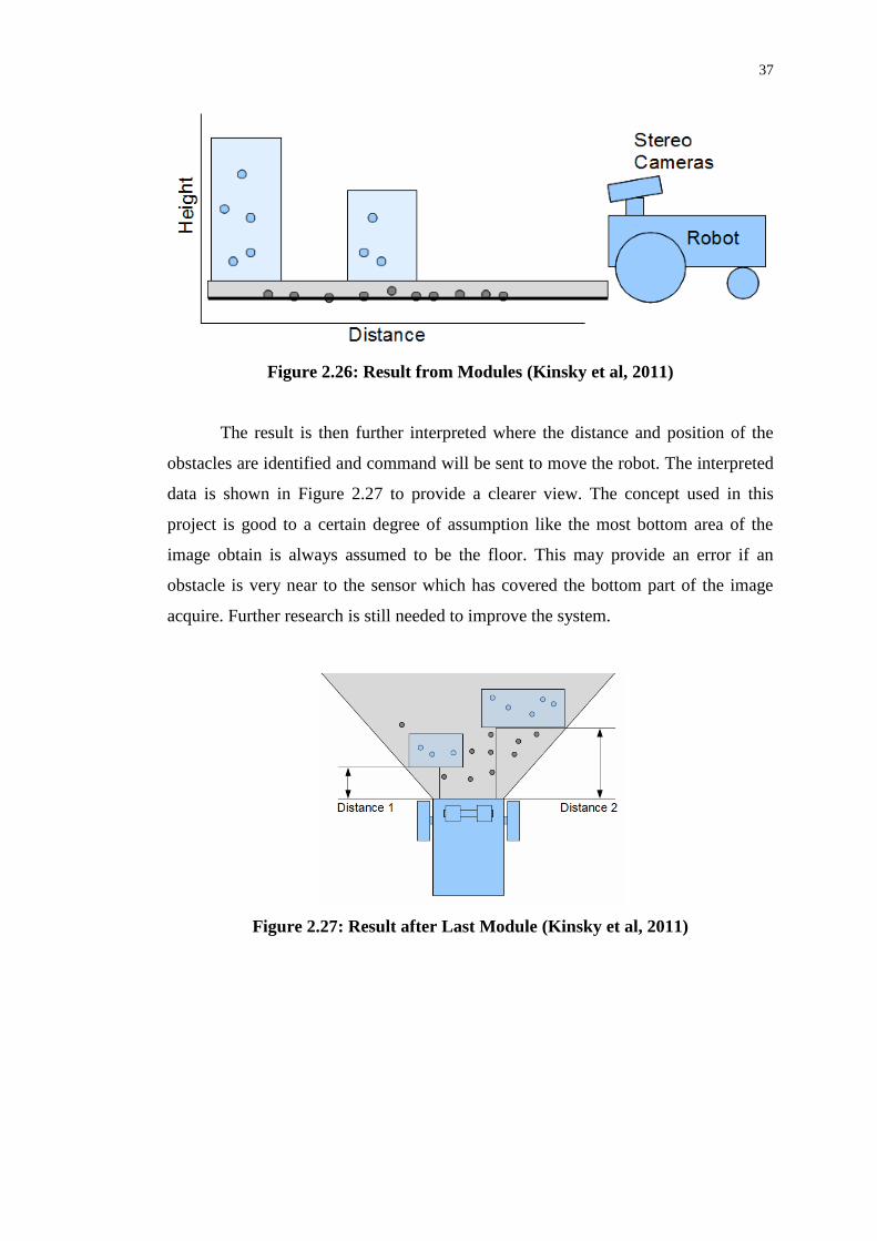
detected by a mobile robot. It is clearly shows in Figure 2.26 where the bottom 10
points highlighted in black is the floor.
Next stage will be the determination of the obstacle points. In this report, the
authors assume the points above the ground plane that exceed the preset distance as
the obstacle points. Figure 2.26 shows that points out of the black shaded box are the
obstacle points. Once the obstacle points have clearly defined, the next module will
combine the points which are close to each other into a cluster that represent as one
obstacle. Blue boundaries are used to frame the obstacle points as shown in Figure
2.26 where there will be two obstacles in the example.
37
Figure 2.26: Result from Modules (Kinsky et al, 2011)
The result is then further interpreted where the distance and position of the
obstacles are identified and command will be sent to move the robot. The interpreted
data is shown in Figure 2.27 to provide a clearer view. The concept used in this
project is good to a certain degree of assumption like the most bottom area of the
image obtain is always assumed to be the floor. This may provide an error if an
obstacle is very near to the sensor which has covered the bottom part of the image
acquire. Further research is still needed to improve the system.
Figure 2.27: Result after Last Module (Kinsky et al, 2011)

38
CHAPTER 3
3 METHODOLOGY
3.1 Introduction
Obstacle detection system consists of two hardware, sensor and microcontroller that
provide the intelligence of “see and observe” to the intelligence semi-automated
wheelchair. After the study of other existed research projects, vision sensor like
human eye plays the initial role where the situation of environment surround is being
identified. Ultrasonic sensor was the choice for this project for the intelligence semi-
automated wheelchair. Besides that, PIC Microcontroller was considered as the
programming hardware for this project. It is common that MPLAB is use to program
as this software is coupled with PIC Microcontroller. After that, the process of
mechanical and electronic developments was presented in the following section.
Finally, the concept and algorithm was discussed as the last section.
3.2 Ultrasonic Sensor
Ultrasonic sensor was the choice in this project due to its characteristics that suit this
project. The detect range from ultrasonic sensor was consider sufficient for obstacle
detection system. Sensor with far range like laser may assume to be overdesign for
this project. Besides, a wide spread detection area in short distance provided the
advantage to the robot to “observe” more about its front area. Moreover, ultrasonic
sensor provided simple data which can be process with a small microcontroller only.
39
Camera with computer as the processor will make the wheel chair become bulky and
heavy. Lastly, ultrasonic sensor was the most economical among all those vision
sensors discussed previously. This will then made the wheelchair design more
affordable to everyone.
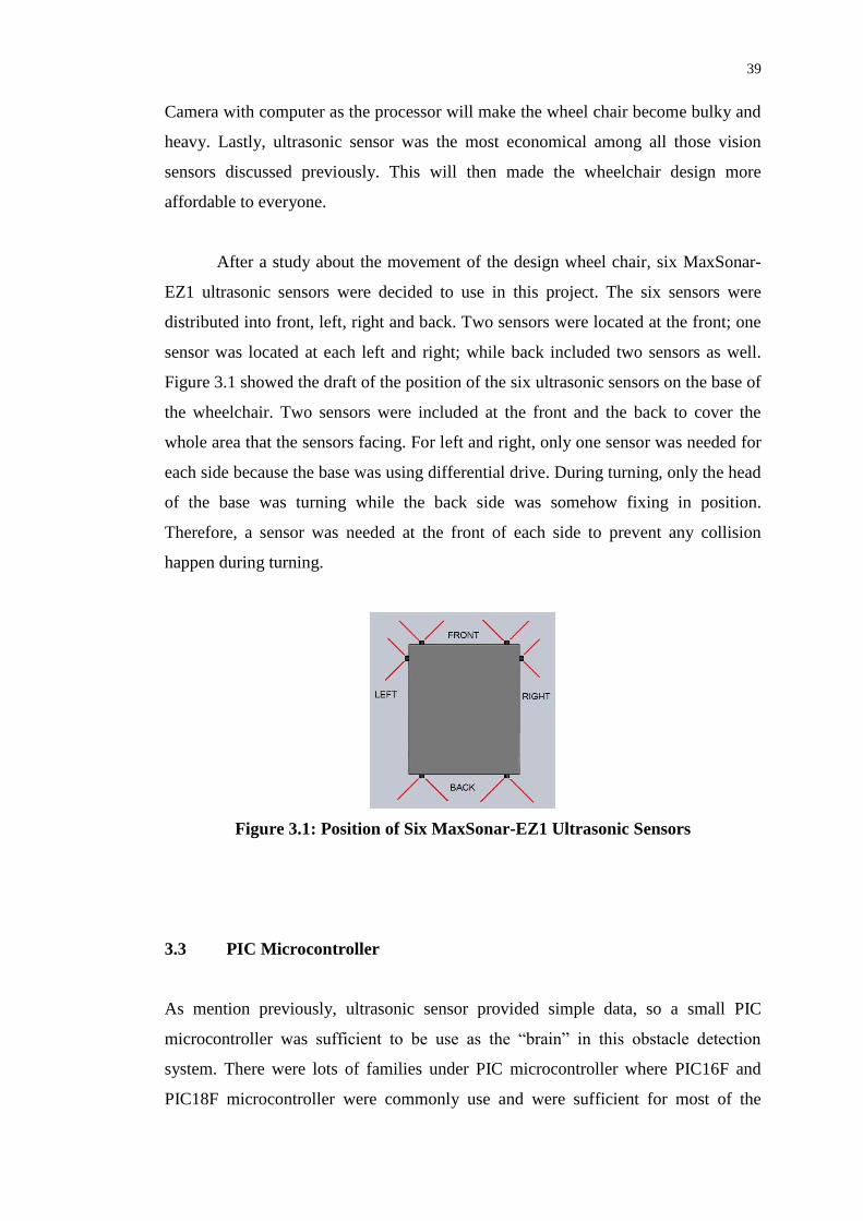
After a study about the movement of the design wheel chair, six MaxSonar-
EZ1 ultrasonic sensors were decided to use in this project. The six sensors were
distributed into front, left, right and back. Two sensors were located at the front; one
sensor was located at each left and right; while back included two sensors as well.
Figure 3.1 showed the draft of the position of the six ultrasonic sensors on the base of
the wheelchair. Two sensors were included at the front and the back to cover the
whole area that the sensors facing. For left and right, only one sensor was needed for
each side because the base was using differential drive. During turning, only the head
of the base was turning while the back side was somehow fixing in position.
Therefore, a sensor was needed at the front of each side to prevent any collision
happen during turning.
Figure 3.1: Position of Six MaxSonar-EZ1 Ultrasonic Sensors
3.3 PIC Microcontroller
As mention previously, ultrasonic sensor provided simple data, so a small PIC
microcontroller was sufficient to be use as the “brain” in this obstacle detection
system. There were lots of families under PIC microcontroller where PIC16F and
PIC18F microcontroller were commonly use and were sufficient for most of the
40
robotic application. PIC24 and 33 may make the design of this project overdesign.
Therefore, PIC18F4520 was chosen for this project due to its characteristic.
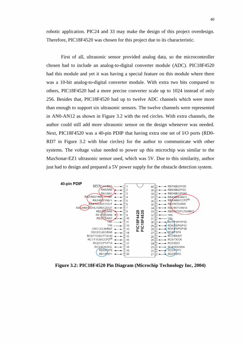
First of all, ultrasonic sensor provided analog data, so the microcontroller
chosen had to include an analog-to-digital converter module (ADC). PIC18F4520
had this module and yet it was having a special feature on this module where there
was a 10-bit analog-to-digital converter module. With extra two bits compared to
others, PIC18F4520 had a more precise converter scale up to 1024 instead of only
256. Besides that, PIC18F4520 had up to twelve ADC channels which were more
than enough to support six ultrasonic sensors. The twelve channels were represented
in AN0-AN12 as shown in Figure 3.2 with the red circles. With extra channels, the
author could still add more ultrasonic sensor on the design whenever was needed.
Next, PIC18F4520 was a 40-pin PDIP that having extra one set of I/O ports (RD0-
RD7 in Figure 3.2 with blue circles) for the author to communicate with other
systems. The voltage value needed to power up this microchip was similar to the
MaxSonar-EZ1 ultrasonic sensor used, which was 5V. Due to this similarity, author
just had to design and prepared a 5V power supply for the obstacle detection system.
Figure 3.2: PIC18F4520 Pin Diagram (Microchip Technology Inc, 2004)

41
3.4 Mechanical Development
Since this project was focusing on designing the systems for autonomous wheelchair,
a prototype of a wheelchair was enough to reduce the research cost. SolidWorks is
3D CAD design software that planned to use by the author to create the mechanical
design. It was very user friendly where author who was not specialty in mechanical
design field was still able to learn and pick up with the software.
Before any mechanical design was started, the author looked into the design
of motorized wheelchair that available at the market. From the study, the author
found out that most of the designs somehow separated the wheelchair into two parts,
the base and the chair. The base contained most of the components of the motorized
wheelchair like motor, wheels, battery and the control unit. On the other hand, the
chair part included the chair itself and the user interface like joystick. Obstacle
detection system was more to automated system and did not need any user interface
to control the system. Therefore, the design for this project was focusing on the base
only but not the chair design. Fabrication of the prototype will be carried out by the
author together with the members who were in charge in other systems of the
intelligence semi-automated wheelchair.
3.5 Electronics Development
As mention previously, PIC18F4520 microcontroller was chosen as the core
controller of the obstacle detection system. Six ultrasonic sensors were used in the
system to detect the obstacle. Next, this system was going to combine with the
driving system and navigation system of the wheelchair, so communication between
the systems was needed. Besides, an indicator to show the specific sensor that detects
an obstacle was planned to include for the ease of research study.
Similar to mechanical development, Eagle PCB software was used to design
the PCB circuit board. Schematic can be draw with this software to complete the
circuit of the system. Most of the electronics components were included in the
42
software with the correct dimension to ease the process. If the component was not in
the library, user could create the library with the software and included it in the
schematic. After that, the schematic can be converted into the PCB board layout. All
the components included in the schematic will display on the PCB board layout and
the user just dragged and placed to arrange the PCB board design.
3.6 Concept and Algorithm
This section was going to talk about the concepts and algorithms that going to apply
on this project for the obstacle detection system. In this project, concept used and
algorithm design shall obey the requirements shown in the list below in order to
achieve the objectives stated previously:
detect obstacle and send specific signal to the driving system to avoid the
obstacle
the algorithm clear about the size and shape of the system structure so that the
it will not collide with the obstacle when travelling
the algorithm always clear with the situation of the system surrounding
the algorithm shall provide a smooth travelling to maintain the user
comfortable
the algorithm shall make the system stop if there is obstacle that too near to
the system
the algorithm shall able to handle both static and moving obstacle
After study on other concepts and algorithms used by other similar project,
edge detection concept was suitable in this project circumstance. As discussed
previously, edge detection concept allows the system to determine where the edge of
the obstacle is. Then, the system will steer around the obstacle by turning left off the
left vertical edge or turning right off the right vertical edge. The choice of this
concept was highly base on the travelling method of the wheelchair. There were two
travelling modes design for the semi-automated wheelchair in this project.
43
First mode will be automatic mode where the wheelchair was travelling by
line following as designed in the navigation system. There will be a special path
provided for the wheelchair to travel around the building. The obstacle detection
system played the role in detecting obstacle that blocking the wheelchair path and
then send signal to the driving system to avoid the obstacle. The flow chart in Figure
3.3 was showing the working principle of this mode. Initially, the wheelchair was
moving with navigation system that following the track provided that aligned with
the left wall. This was set based on the traffic in Malaysia where car was always
taking the left lane when travelling. Once an obstacle was detected blocking the path
line, the obstacle detection system will take over the wheelchair control. As shown in
the flow chart, the wheelchair would slow down and then the lean right signal was
sent to the driving system to detect the obstacle edge. At this stage, edge detection
concept was used and identified the position of the edge. After that, the same signal
was continuous sent to the driving system for a short period so that the whole
wheelchair was having enough space to pass the edge without collision.
Once the edge had passed by, a forward signal was sent to the driving system
to move the wheelchair. At this stage, the left sensor was activated to detect another
edge of the obstacle which was considered as the end edge. After that, lean left signal
was sent and the wheelchair started to lean left. Toward the end, the wheelchair will
definitely avoid the obstacle and then back to the track prepared by the navigation
system. The navigation system will then take over the wheelchair control.
The algorithm used in this system can be explained as sensory based
algorithm where the system was directly used the information from the sensor to
response accordingly (Kamon & Rivlin, 1995). It also called as local planning
algorithm. The algorithm for the automatic mode will be as shown below:
1. Detect obstacle bloking the front path.
2. Slow down the speed and start to lean to the right.
a. Front sensor detect obstacle edge. Go to step 3.
b. If not. Repeat with step 2.
3. Steer another short period to the right.
4. Move forward with slightly to the left steer.
44
a. Front sensor detect obstacle. Go to step 3.
b. If no. Go to step 5.
5. Move forward with another short period.
6. Move forward with slightly left steering.
a. Detect line path (navigation system). Go to step 7.
b. If no. Repeat step 6.
7. Navigation system takes over the control.
The second mode was semi-automatic mode where the wheelchair was
controlled by the user to travel around, while the obstacle detection system worked
as the safety support element. Once an obstacle was detected, the obstacle detection
system cut off the user control and the wheelchair will then come to a stop. At this
stage, the user control was limited from the direction to the obstacle. For example, if
the obstacle was detected to be at the front of the wheelchair, the user was only able
to control left or right turning without any forward motion. Once the obstacle was no
longer blocking the way, the normal user control will reactivate back. The process
was clearly shown in the flow chart in Figure 3.4.
The algorithm used for semi automatic mode was presented as shown below:
1. Detect obstacle bloking the travel direction.
2. Slow down and stop the wheelchair.
3. Limit the user control from the direction of the obstacle present.
a. If obstacle still present in the sensor range. Repeat step 3.
b. If no. Go to step 4.
4. Normal user control is resume

45
Figure 3.3: Automated Mode

46
Figure 3.4: Semi-Automated Mode

47
CHAPTER 4
4 RESULTS AND DISCUSSIONS
4.1 Mechanical Development
Initially, the position of the wheels was very important to have a stable base. In the
first concept design, two differential wheels and two caster wheels were used in this
project. Differential drive was used due to its simplicity of driving control. Therefore,
each differential wheel was mounted with one DC motor. Caster wheel was chosen
as the front wheel so that the front part was free to move in any direction depending
to the driving wheel. Besides wheels and motors, battery was needed as the power
supply to the whole system. Since the two batteries had to remove from the base to
be charge from time to time, it was design to place above the motor. The batteries
were chosen to place together with the motor in order to create more space for the
control unit boards. A battery box was also design to hold both batteries, so that it
was easier to remove the batteries in one from the base. Figure 4.1 below showed the
first conceptual design in this project.
Figure 4.1: Mechanical Design Version 1

48
Next, the author found out that the first design was having weight distribution
problem, where the back part of the base was fill with the two main components of
the system that were heavy. The front base may lifted up when the base was having
acceleration. Therefore, the batteries were shift to the front to counter weight the
motors. At the same time, it was still obey the condition where the batteries were
ease to remove. Besides that, the mounting of the battery holder was complicated, so
the author did not included it in the second design. A special space was created to
place the battery with L-shape plate, so that the battery was stay in position when the
base was moving. Since the chair was above the base, it made the design complicated
if the batteries had to remove from above. Therefore, instead of placing the front
plywood permanently, the author designs the front plywood to be flexible so that it
could be open as shown in Figure 4.2. The middle space between the motor and
battery was reserved for the control unit boards.
Figure 4.2: Mechanical Design Version 2
The design was carried on with the ultrasonic sensor mounting for the
obstacle detection system. As mention previously, there were six ultrasonic sensors
in total to be mounted on the base with the distribution, two at the front, one at each
of the left and right and another two at the back. In order to have a simple design, the
ultrasonic sensors were design to mount on the plywood. Hole would be drill on the
plywood so that the ultrasonic sensor could directly mount on it as shown in Figure
4.3. This design was constructed out as shown in Figure 4.4.

49
Figure 4.3: Mechanical Design Version 3 with SolidWorks
Figure 4.4: Constructed Mechanical Design Version 3
Once the design version 3 was constructed, few tests were done on the design.
First of all, the most important component, ultrasonic sensor was tested.
Unfortunately, the reading from the ultrasonic sensor did not achieve the expectation.
Although there was no obstacle in front of the ultrasonic sensor, the sensor provided
a reading of 240.2 mV. This showed that it was only able to detect an obstacle that
was lower than 0.6 m away from the base. This distance was considers near and the
base would had not enough time to response to avoid the obstacle. The factor on this
problem was the height of the sensor on the base which was only 16.5 cm. In order to
overcome this problem, the height of the sensor mounting had to be increased, but
this would then cause the design became not practical. Therefore, the author decided
to mount the sensor on top of the base with a small tilt on the sensor holder as shown
in Figure 4.5 and Figure 4.6. This increased the distance that the base able to
measure, at the same time, it did not influence the base size. With an approximate 10
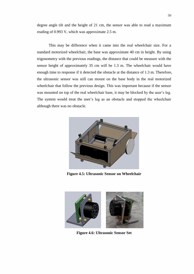
50
degree angle tilt and the height of 21 cm, the sensor was able to read a maximum
reading of 0.993 V, which was approximate 2.5 m.
This may be difference when it came into the real wheelchair size. For a
standard motorized wheelchair, the base was approximate 40 cm in height. By using
trigonometry with the previous readings, the distance that could be measure with the
sensor height of approximately 35 cm will be 1.3 m. The wheelchair would have
enough time to response if it detected the obstacle at the distance of 1.3 m. Therefore,
the ultrasonic sensor was still can mount on the base body in the real motorized
wheelchair that follow the previous design. This was important because if the sensor
was mounted on top of the real wheelchair base, it may be blocked by the user’s leg.
The system would treat the user’s leg as an obstacle and stopped the wheelchair
although there was no obstacle.
Figure 4.5: Ultrasonic Sensor on Wheelchair
Figure 4.6: Ultrasonic Sensor Set
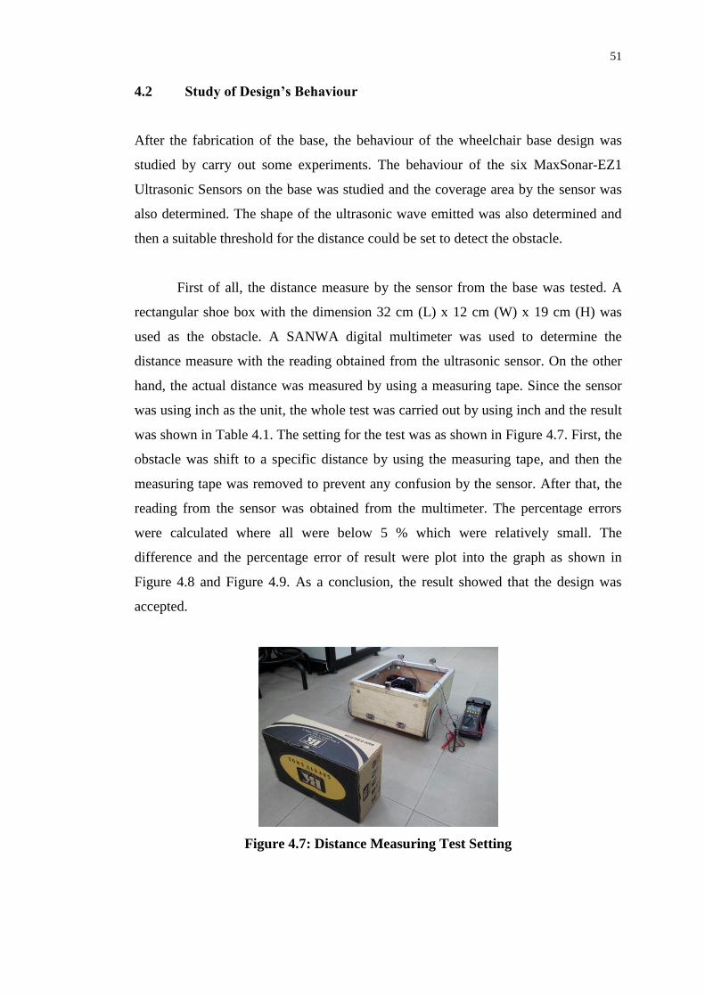
51
4.2 Study of Design’s Behaviour
After the fabrication of the base, the behaviour of the wheelchair base design was
studied by carry out some experiments. The behaviour of the six MaxSonar-EZ1
Ultrasonic Sensors on the base was studied and the coverage area by the sensor was
also determined. The shape of the ultrasonic wave emitted was also determined and
then a suitable threshold for the distance could be set to detect the obstacle.
First of all, the distance measure by the sensor from the base was tested. A
rectangular shoe box with the dimension 32 cm (L) x 12 cm (W) x 19 cm (H) was
used as the obstacle. A SANWA digital multimeter was used to determine the
distance measure with the reading obtained from the ultrasonic sensor. On the other
hand, the actual distance was measured by using a measuring tape. Since the sensor
was using inch as the unit, the whole test was carried out by using inch and the result
was shown in Table 4.1. The setting for the test was as shown in Figure 4.7. First, the
obstacle was shift to a specific distance by using the measuring tape, and then the
measuring tape was removed to prevent any confusion by the sensor. After that, the
reading from the sensor was obtained from the multimeter. The percentage errors
were calculated where all were below 5 % which were relatively small. The
difference and the percentage error of result were plot into the graph as shown in
Figure 4.8 and Figure 4.9. As a conclusion, the result showed that the design was
accepted.
Figure 4.7: Distance Measuring Test Setting

52
Table 4.1: Distance Measuring Test Result
No Actual
Distance, da (in)
Sensor Reading
(mV)
Calculated Distance, dc
(in)
Difference (in)
Error (%)
1 12.0 124.0 12.4 0.4 3.33
2 18.0 182.0 18.2 0.2 1.11
3 24.0 229.8 23.0 1.0 4.25
4 30.0 288.5 28.9 1.2 3.83
5 36.0 346.6 34.7 1.3 3.72
6 42.0 405.0 40.5 1.5 3.57
7 48.0 463.0 46.3 1.7 3.54
8 54.0 520.0 52.0 2.0 3.70
9 60.0 584.0 58.4 1.6 2.67
10 66.0 637.0 63.7 2.3 3.48
11 72.0 696.0 69.6 2.4 3.33
12 78.0 765.0 76.5 1.5 1.92
Figure 4.8: Graph of Actual Distance vs Measured Distance
Figure 4.9: Graph of Percentage Error for Distance Measuring Test

53
Second test was about the wave propagation and the coverage area of the
sensor. From the datasheet, the propagation angles of B and C were considered. By
using trigonometry equation, the angle of propagation of B was approximate 31.9˚,
while C was approximate 39.3˚. By drawing the propagation areas on a mah-jong
paper, the test was carried out as shown in Figure 4.10. Beside the specific angles,
angles from 0˚-180˚ with the resolution 15˚ were also included. The similar obstacle
was use in this test and it was place according to the angle set. In each angle, the
obstacle was place in four different distances to obtain the distance measured by the
sensor. Table 4.2 showed the result of the experiment.
The rows with yellow shaded represented the angle for the C propagation
angle as stated in the sensor’s datasheet. While, blue shaded rows were the B
propagation angle. Supposedly, according to the information from the datasheet, the
sensor would not detect any obstacle that was placed beyond the purple line as
shown in Figure 4.11. The shaded area in the Figure 4.11 and the thicker bolder in
Table 4.2 showed the detected area according to the sensor datasheet. Surprisingly,
after the experiment, the author found out that when the obstacle was placed at the
angle of 60˚ and 120˚, it was still able to detect the obstacle as shown in Table 4.2.
This make the system more reliable as the sensor coverage was wider compared to
the datasheet, which mean that it was able to obtain more information from the
surrounding. Percentage errors were calculated by using the difference between the
actual distance and measured distance for the detected area (60˚-120˚). Table 4.3
showed the result of the percentage error and a graph was prepared as shown in
Figure 4.12 to show the results in one. The result showed that the maximum
percentage error was 5% which was still considered as relatively low. In conclusion,
the result showed that the design was satisfied.

54
Figure 4.10: Sensor Coverage Test Setting
Figure 4.11: Mahjong Paper with Angles Setting
Table 4.2: Sensor Coverage Test Result
Distance (in)
15 30 45 60
Angle (˚)
0 No No No No
15 No No No No
30 No No No No
45 No No No No
60 14.30 28.70 43.30 57.90
70.35 (C) 14.42 28.75 43.50 56.90
74.06 (B) 14.27 28.77 43.40 57.00
75 14.28 28.80 43.30 56.90
90 14.30 28.80 43.50 57.00
105 14.32 28.77 43.40 57.00
105.90 (B) 14.32 28.75 43.40 57.00
109.65 (C) 14.28 28.75 43.40 57.00
120 15.20 29.80 43.40 58.80
135 No No No No
150 No No No No
165 No No No No
180 No No No No

55
Table 4.3: Percentage Error for Sensor Coverage Test Result
Angle (˚)
Actual Distance (15 in)
Measured
Distance
Difference
(in)
Error
(%)
60 14.30 0.7 4.67
70.35 (C) 14.42 0.6 3.87
74.06 (B) 14.27 0.7 4.87
75 14.28 0.7 4.80
90 14.30 0.7 4.67
105 14.32 0.7 4.53
105.90 (B) 14.32 0.7 4.53
109.65 (C) 14.28 0.7 4.80
120 15.20 0.2 1.33
Angle (˚)
Actual Distance (30 in)
Measured
Distance
Difference
(in)
Error
(%)
60 28.70 1.3 4.33
70.35 (C) 28.75 1.3 4.17
74.06 (B) 28.77 1.2 4.10
75 28.80 1.2 4.00
90 28.80 1.2 4.00
105 28.77 1.2 4.10
105.90 (B) 28.75 1.3 4.17
109.65 (C) 28.75 1.3 4.17
120 29.80 0.2 0.67
Angle (˚)
Actual Distance (45 in)
Measured
Distance
Difference
(in)
Error
(%)
60 43.30 1.7 3.78
70.35 (C) 43.50 1.5 3.33
74.06 (B) 43.40 1.6 3.56
75 43.30 1.7 3.78
90 43.50 1.5 3.33
105 43.40 1.6 3.56
105.90 (B) 43.40 1.6 3.56
109.65 (C) 43.40 1.6 3.56
120 43.40 1.6 3.56

56
Angle (˚)
Actual Distance (60 in)
Measured
Distance
Difference
(in)
Error
(%)
60 57.90 2.1 3.50
70.35 (C) 56.90 3.1 5.17
74.06 (B) 57.00 3.0 5.00
75 56.90 3.1 5.17
90 57.00 3.0 5.00
105 57.00 3.0 5.00
105.90 (B) 57.00 3.0 5.00
109.65 (C) 57.00 3.0 5.00
120 58.80 1.2 2.00
Figure 4.12: Graph of Percentage Error for Sensor Coverage Test
4.3 Electronics Development
As mention previously, six ultrasonic sensors were used in the system, so six ADC
pins of the microcontroller were needed as the input of the system. In order to have
communication with other system, ten I/O ports were included with the pin headers
for connection purpose. On the other hand, six I/O ports were set as output to be used
as the indicator. Besides that, CCP1 and CCP2 pins under PWM module were
included with pin headers as well so that the author was able to control and test with
the driving motors before combining with the driving system. Another two I/O ports,
RD0 and RD1 were included to control the direction of the driving motor. Lastly, the

57
author included a 10 ways box header in the circuit design to ease the programming
process.
In designing the obstacle detection system board, all of the components were
included in the Eagle library except the microcontroller. PIC18F4455 was taken to
replace PIC18F4520 because both were having the similar set of pins. The schematic
design and the board design for the obstacle detection system were as shown in
Figure 4.13. The board was fabricated out by the author and the product was as
shown in Figure 4.14.
Besides that, a power board circuit for the whole wheelchair system was also
designed by author. A readymade 5V/3.3V power stick from Cytron Technologies
was used to convert the power source 12V from the battery to the specific voltages.
The outputs from the power stick were duplicated out into few molex connectors to
supply power. At the same time, 24V from the battery was duplicated out into two
connectors for the driving motors and 12V for DC motors. Figure 4.15 showed the
schematic and PCB board design for the power board design. Since the power stick
was readymade, it did not included in the software library, so the author created the
library according to the dimension. Similar to the connector for the 12V and 24V, the
author created the library according to the dimension. Once the PCB design was
done, the board was fabricated out by the author and the product was as shown in
Figure 4.16.
Next, the author came out with a simple design circuit with six LEDs and six
4.7kΩ resistors to work as the indicator for the six ultrasonic sensors. Figure 4.17
showed the simple design where the LEDs were arranged according to the sensors
position. The top two LEDs in Figure 4.17 represented the front sensors. Follow on,
the left and right LED that represented the left and right of the sensors respectively.
Next, the final bottom two sensors represented the back sensors of the wheelchair.
With this indicator, the author was able to determine which sensor was detecting an
obstacle and which was not. This eased the study of the system behaviour.

58
Figure 4.13: Schematic and PCB Board of Obstacle Detection System
Figure 4.14: Obstacle Detection System Board
Figure 4.15: Schematic and PCB Board of Power Board
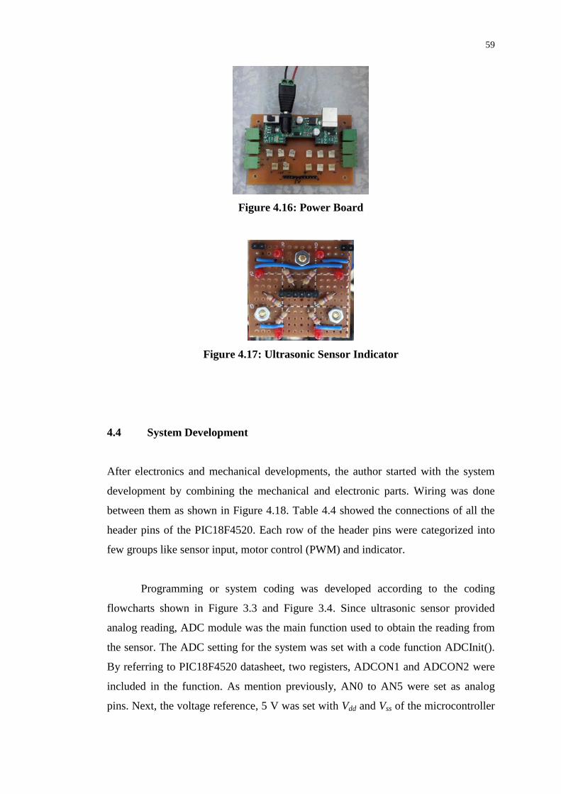
59
Figure 4.16: Power Board
Figure 4.17: Ultrasonic Sensor Indicator
4.4 System Development
After electronics and mechanical developments, the author started with the system
development by combining the mechanical and electronic parts. Wiring was done
between them as shown in Figure 4.18. Table 4.4 showed the connections of all the
header pins of the PIC18F4520. Each row of the header pins were categorized into
few groups like sensor input, motor control (PWM) and indicator.
Programming or system coding was developed according to the coding
flowcharts shown in Figure 3.3 and Figure 3.4. Since ultrasonic sensor provided
analog reading, ADC module was the main function used to obtain the reading from
the sensor. The ADC setting for the system was set with a code function ADCInit().
By referring to PIC18F4520 datasheet, two registers, ADCON1 and ADCON2 were
included in the function. As mention previously, AN0 to AN5 were set as analog
pins. Next, the voltage reference, 5 V was set with Vdd and Vss of the microcontroller

60
to simplify the circuit. Since the microcontroller provided a 10 bits ADC module, the
author calculated the resolution with the equation as shown below and the result was
1 bit represented 4.88mV.
102
refVresolution (4.1)
where
Vref = voltage reference, V
According to the sensor datasheet, the sensor provided a voltage output with a
range from 0V to 2.55V. Since the maximum output voltage was only 2.55V, it did
not use up all the 1024 bits (210
) of the ADC module. By dividing the maximum
voltage with the resolution obtained previously, it gives a result of 522.54 which was
round off to 522 bits. This showed that the microcontroller would read the sensor
reading in bit form from 0 bit to 522 bit that represented the distance detected.
According to the datasheet, the sensor was having a resolution of 10mV/in. This
means that every changes of the sensor reading (1 in) would make an approximate 2
bits change in the microcontroller. As a conclusion, the resolution of
microcontroller’s bits per inch was approximate 2bits/in. This resolution was
determined to ease the author in developing the coding especially in setting the
distance threshold to detect obstacle.
Next, the acquisition time in ADC module was a very important factor. The
acquisition time represented the time taken for the microcontroller to take a reading.
There were some requirements to obey when setting this factor like the minimum and
maximum of A/D conversion clock, TAD which were 0.7µs and 25µs respectively.
Since there were six sensors to be read in one time, the author set the acquisition time
as fast as possible. With the minimum requirement of TAD, the A/D conversion clock
was set to FOSC/32. By using the equation as shown below, TAD was calculated to be
1.6µs with 20MHz as the oscillator clock frequency. The result obeyed the
requirement where 1.6µs was higher than 0.7 µs.
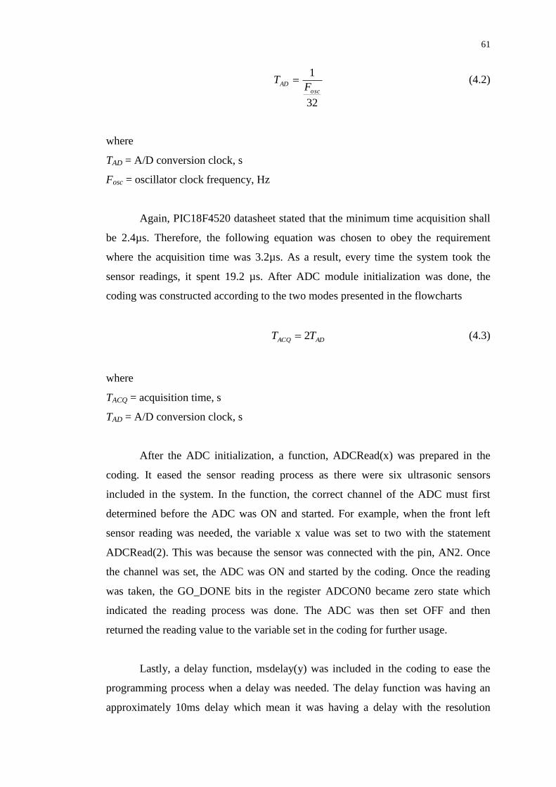
61
32
1
oscAD F
T (4.2)
where
TAD = A/D conversion clock, s
Fosc = oscillator clock frequency, Hz
Again, PIC18F4520 datasheet stated that the minimum time acquisition shall
be 2.4µs. Therefore, the following equation was chosen to obey the requirement
where the acquisition time was 3.2µs. As a result, every time the system took the
sensor readings, it spent 19.2 µs. After ADC module initialization was done, the
coding was constructed according to the two modes presented in the flowcharts
ADACQ TT 2 (4.3)
where
TACQ = acquisition time, s
TAD = A/D conversion clock, s
After the ADC initialization, a function, ADCRead(x) was prepared in the
coding. It eased the sensor reading process as there were six ultrasonic sensors
included in the system. In the function, the correct channel of the ADC must first
determined before the ADC was ON and started. For example, when the front left
sensor reading was needed, the variable x value was set to two with the statement
ADCRead(2). This was because the sensor was connected with the pin, AN2. Once
the channel was set, the ADC was ON and started by the coding. Once the reading
was taken, the GO_DONE bits in the register ADCON0 became zero state which
indicated the reading process was done. The ADC was then set OFF and then
returned the reading value to the variable set in the coding for further usage.
Lastly, a delay function, msdelay(y) was included in the coding to ease the
programming process when a delay was needed. The delay function was having an
approximately 10ms delay which mean it was having a delay with the resolution

62
10ms. The variable, y value represented the multiplier value of the delay. For
example, in order to achieve a 50ms delay, the value x was set to be five with the
statement msdelay(5).
Figure 4.18: Combination between Electronics and Mechanical
Table 4.4: Microcontroller Pin Assignment
Ultrasonic Sensor Input Sensor ON/OFF Control
Pin Position Pin Position
AN0 Front Right (FR) RC6 Back Right (BR)
AN1 Right (R) RC5 Back Left (BL)
AN2 Front Left (FL) RC4 Front Left (FL)
AN3 Left (L) RD3 Front Right (FR)
AN4 Back Left (BL) RD2 Off Automated Mode
(Input from driving system)
AN5 Back Right (BR)
Indicator Motor Control Driving System
Pin Position Pin Motor Pin Driving Signal
RB7 Left (L) CCP1 Motor Speed 1 RD7 Forward
RB6 Back Left (BL) CCP2 Motor Speed 2 RD6 Left
RB5 Front Left (FL) RD0 Motor Direction 1 RD5 Right
RB4 Front Right (FR) RD1 Motor Direction 2 RD4 Reverse
RB3 Back Right (BR) RC7 Mode Input
RB2 Right (R)
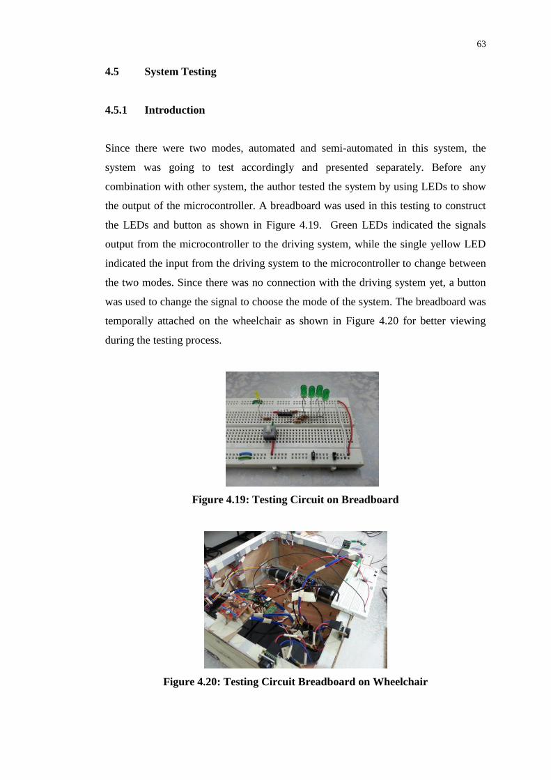
63
4.5 System Testing
4.5.1 Introduction
Since there were two modes, automated and semi-automated in this system, the
system was going to test accordingly and presented separately. Before any
combination with other system, the author tested the system by using LEDs to show
the output of the microcontroller. A breadboard was used in this testing to construct
the LEDs and button as shown in Figure 4.19. Green LEDs indicated the signals
output from the microcontroller to the driving system, while the single yellow LED
indicated the input from the driving system to the microcontroller to change between
the two modes. Since there was no connection with the driving system yet, a button
was used to change the signal to choose the mode of the system. The breadboard was
temporally attached on the wheelchair as shown in Figure 4.20 for better viewing
during the testing process.
Figure 4.19: Testing Circuit on Breadboard
Figure 4.20: Testing Circuit Breadboard on Wheelchair
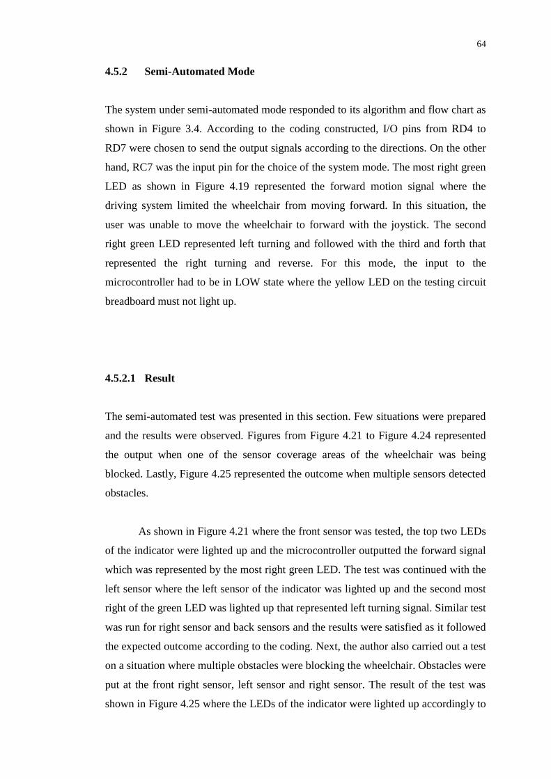
64
4.5.2 Semi-Automated Mode
The system under semi-automated mode responded to its algorithm and flow chart as
shown in Figure 3.4. According to the coding constructed, I/O pins from RD4 to
RD7 were chosen to send the output signals according to the directions. On the other
hand, RC7 was the input pin for the choice of the system mode. The most right green
LED as shown in Figure 4.19 represented the forward motion signal where the
driving system limited the wheelchair from moving forward. In this situation, the
user was unable to move the wheelchair to forward with the joystick. The second
right green LED represented left turning and followed with the third and forth that
represented the right turning and reverse. For this mode, the input to the
microcontroller had to be in LOW state where the yellow LED on the testing circuit
breadboard must not light up.
4.5.2.1 Result
The semi-automated test was presented in this section. Few situations were prepared
and the results were observed. Figures from Figure 4.21 to Figure 4.24 represented
the output when one of the sensor coverage areas of the wheelchair was being
blocked. Lastly, Figure 4.25 represented the outcome when multiple sensors detected
obstacles.
As shown in Figure 4.21 where the front sensor was tested, the top two LEDs
of the indicator were lighted up and the microcontroller outputted the forward signal
which was represented by the most right green LED. The test was continued with the
left sensor where the left sensor of the indicator was lighted up and the second most
right of the green LED was lighted up that represented left turning signal. Similar test
was run for right sensor and back sensors and the results were satisfied as it followed
the expected outcome according to the coding. Next, the author also carried out a test
on a situation where multiple obstacles were blocking the wheelchair. Obstacles were
put at the front right sensor, left sensor and right sensor. The result of the test was
shown in Figure 4.25 where the LEDs of the indicator were lighted up accordingly to

65
the sensors and the microcontroller outputted the signals to limit the motion of
forward, left and right. As a conclusion, the semi-automated system was working and
the results were satisfied.
Figure 4.21: Front Sensor Test
Figure 4.22: Left Sensor Test
Figure 4.23: Right Sensor Test

66
Figure 4.24: Back Sensor Test
Figure 4.25: Multiple Sensors Test
4.5.3 Automated Mode
After the testing on the semi-automated mode, this section presented the automated
mode test. Similar to semi-automated mode, the indicator and the testing circuit
breadboard were used. In this mode, the indicator instead of only showing the
specific position sensor detected an obstacle or not, it also used to show the stage of
the automated system. Since both automated and semi-automated would never work
at the same time, the same I/O ports from semi-automated mode were used. The
similar signals were sent by the microcontroller to control the wheelchair motion.
The only different was semi-automated mode limit the specific motion, but
automated mode wants the driving system to response according to the signal
provided. For example, if forward signal was sent by the obstacle detection system,
the driving system must run the wheelchair in a forward motion straight to the front.
As opposite from semi-automated mode, the input of the microcontroller must set to
67
HIGH state in order run the system in automated mode. The yellow LED on the
testing circuit must light up as shown in Figure 4.26.
4.5.3.1 Result
The result for automated test was presented in this section where the concept as
shown in the flow chart in Figure 3.3 was showed. Different from the semi-
automated mode, automated mode was a process in avoiding an obstacle that
blocking the front path during navigation. Therefore, instead of showing different
situations, the system was tested with the whole process and the results were shown
from Figure 4.26 to Figure 4.29.
The whole process was started when the front sensor detected an obstacle.
This activated the system to overwrite the navigation system to control the
wheelchair motion. The obstacle detection system was communicated with the
driving system. The two front LEDs of the indicator will lighted up as shown in
Figure 4.26 once it detected an obstacle at the front. As stated in the automated mode
algorithm, the wheelchair would slow down and then leaned right until the front left
sensor detected the obstacle’s edge. During the lean right motion (second left green
LED), the front right LED went off first followed by the front left LED as shown in
third photo of Figure 4.26. Once the front left detected the obstacle’s edge, the
wheelchair remained lean right motion for another two seconds to make sure that it
would not collide with the obstacle during the next motion. Then, the wheelchair was
commanded to move forward until the left sensor detected the obstacle’s edge. This
was why the left LED was lighted up in this stage and the most right green LED
represented the forward signal as shown in 4.27.
The process was carried on until the left sensor detected another obstacle’s
edge that indicated the wheelchair had come to the end of the obstacle. Forward
signal (most right green LED) was sent for four seconds so that the wheelchair was
totally passed the obstacle’s edge. Finally, the wheelchair was instructed to lean left
(second most right green LED) for two seconds followed by forward signal (most

68
right green LED) until the wheelchair was back to the navigation path. All the LEDs
result was showed in Figure 4.28. After that, the navigation system took back the
wheelchair motion control.
Figure 4.26: Automated Test 1
Figure 4.27: Automated Test 2
Figure 4.28: Automated Test 3

69
4.5.4 Discussion on System Test
From the tests presented above, both semi-automated and automated modes were
providing satisfied result. The system did follow the programming with the readings
from ultrasonic sensors and then outputted the wheelchair motion signal accordingly.
Each of the tests had repeated for ten times to ensure that both coding were useable
and reliable. From all the tests, failure did happen on the front or back sensors.
Ultrasonic waveforms from the sensors interrupted each other readings. This
was due to the similar frequency waveform used in MaxSonar-EZ1. For example,
when the front left sensor emitted a waveform and reflected by an obstacle which
was not perpendicular to the sensor, the waveform was then reflected to another
direction toward the front right sensor. With the reflected waveform, the front right
sensor did detect and assumed there was an obstacle located at the front. This
situation was presented in Figure 4.29. In order to overcome this situation, RX pin of
each of the sensors located at the front and back of wheelchair were connected to the
microcontroller of the system. This pin allowed the system to ON/OFF the sensor, so
the two sensors that located at the same row (front or back) were set to ON/OFF
alternatively. For example, if front left sensor was ON, front right sensor would set to
OFF, then front left sensor would take the reading. After that, the front left sensor
was set to OFF, while front right sensor was ON and took its reading. A short delay
was provided so the sensor had enough time (20µs) to startup. With this setting, both
sensors would never ON at the same time. The short delay time was decided to be
30ms after some try an error and testing. Although this method did improve the result,
but it was still having few minor interrupt. This was because the delay time was not
long enough which had to be approximate 0.1s. The system did not provide such a
long delay because it was going to affect the system response which was one of the
main factors in this project.

70
Figure 4.29: Sensor Wave Interruption
4.6 Systems Combination
4.6.1 Introduction
After individual system test, the obstacle detection system was combined with
driving system and navigation system to come out with whole semi-automated
wheelchair design. In semi-automated mode, the obstacle detection system
communicated with the driving system without the interference from the navigation
system. On the other hand, both obstacle detection system and navigation system
took turn to communicate with the driving system by providing the motion signals in
different situation during automated mode. Again, different types of testing were
conducted for both automation and semi-automated modes to study about the system
behaviour and its reliability.
4.6.2 Semi-Automated Mode
This mode was used when the user was manually control the wheelchair motion.
Similar to other existing motorized wheelchair, the driving system included an

71
analog joystick for the user to control the wheelchair motion. As mention previously,
the obstacle detection system worked as the supporter to the user in term of safety. It
helped the user in detecting an obstacle that tended to block the wheelchair and then
prevented the user to control the wheelchair toward the obstacle, which then
prevented collision with the obstacle. The obstacle detection system would send
signals to the driving system to limit the motion control from the user toward the
obstacle direction. For example, when there was an obstacle happened to block at the
front of the wheelchair, the user cannot moved the wheelchair to the front anymore.
The user either controlled the wheelchair in left or right turning, or the reverse
motion to avoid the obstacle. Once the obstacle was no longer blocking the
wheelchair, the forward motion was back to control.
Some tests were run through for the semi-automated system to study the
behaviour of the wheelchair. Four different obstacles were prepared as shown in
Figure 4.30 where the most left was a semi-transparent water bottle with cylindrical
shape, followed by a rectangular shoe box and a larger rectangular CPU box. The
most right obstacle would be a chair with irregular shape. Water bottle was prepared
to represent water bottle and medicine container that occurred in a hospital. On the
other hand, two different sizes of box were tested to observe the system detection
ability in term of size. Lastly, the chair represented any of the furniture and hospital
equipments like trolley that having irregular shape. On the other hand, moving
human represented the moving obstacle for the tests.
First of all, the system was tested in term of the sensor range coverage.
Before the test was carried out to study the system behaviour, trial and error method
was used to determine the best range to be set for the obstacle detection system. The
PC box obstacle was used because it was assumed to be the best obstacle for the
system to be detected. From the test, the front and back range was set to be 20in,
while 15in was set for left and right. A longer range was set for the front because it
was widely used, and the forward motion was more likely to achieve the maximum
speed. Therefore, a longer distance was needed for the wheelchair to come to a stop.
Once the ranges were set, the system was carried on with the other tests.
Since the system limited the motion in four directions, four tests were carried
out for each of the directions with the obstacles prepared. By using a contact
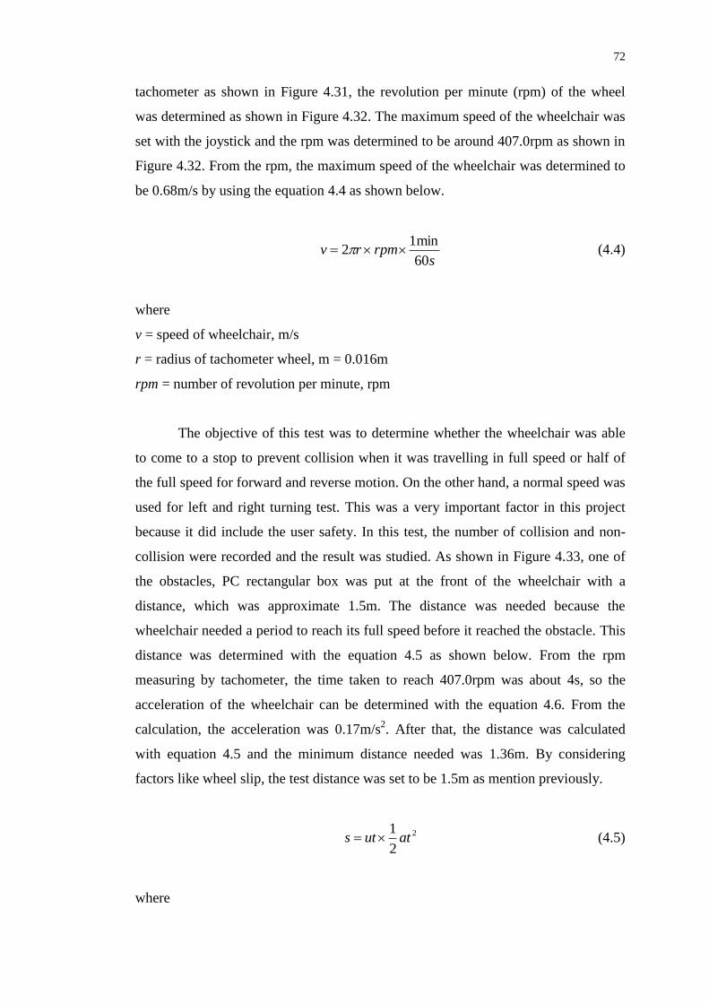
72
tachometer as shown in Figure 4.31, the revolution per minute (rpm) of the wheel
was determined as shown in Figure 4.32. The maximum speed of the wheelchair was
set with the joystick and the rpm was determined to be around 407.0rpm as shown in
Figure 4.32. From the rpm, the maximum speed of the wheelchair was determined to
be 0.68m/s by using the equation 4.4 as shown below.
s
rpmrv60
min12 (4.4)
where
v = speed of wheelchair, m/s
r = radius of tachometer wheel, m = 0.016m
rpm = number of revolution per minute, rpm
The objective of this test was to determine whether the wheelchair was able
to come to a stop to prevent collision when it was travelling in full speed or half of
the full speed for forward and reverse motion. On the other hand, a normal speed was
used for left and right turning test. This was a very important factor in this project
because it did include the user safety. In this test, the number of collision and non-
collision were recorded and the result was studied. As shown in Figure 4.33, one of
the obstacles, PC rectangular box was put at the front of the wheelchair with a
distance, which was approximate 1.5m. The distance was needed because the
wheelchair needed a period to reach its full speed before it reached the obstacle. This
distance was determined with the equation 4.5 as shown below. From the rpm
measuring by tachometer, the time taken to reach 407.0rpm was about 4s, so the
acceleration of the wheelchair can be determined with the equation 4.6. From the
calculation, the acceleration was 0.17m/s2. After that, the distance was calculated
with equation 4.5 and the minimum distance needed was 1.36m. By considering
factors like wheel slip, the test distance was set to be 1.5m as mention previously.
2
2
1atuts (4.5)
where

73
s = distance, m
u = initial velocity, m/s = 0m/s
t = time taken, s
a = acceleration, m/s2
t
uva
(4.6)
where
a = acceleration, m/s2
s = distance, m
u = initial velocity, m/s = 0m/s
t = time taken, s
The setting in Figure 4.33 showed the full speed test for the PC box obstacle
and the result was recorded in Table 4.5. The test was carried on with the half full
speed test with forward motion, and then repeated the both tests with the other
obstacles. Next, the tests were repeated with reverse motion. After that, a normal
speed was used for left and right turning test and the test was also repeated for the
four obstacles. Each of the tests was carried out for thirty times to obtain a better
result for observation. The result obtained was observed and discussed in the next
section
Next, a random moving test was carried out with all the obstacles presented at
the wheelchair surrounding as shown in Figure 4.34. By using the joystick prepared
by the driving system, the wheelchair was controlled to move from an end to another
passing through the obstacles presented randomly. The objective of this test was to
determine the reliability of the obstacle detection system according to a random
obstacle presented from time to time. The random moving test was repeated for thirty
times fore and back and the number of collision and non-collision were recorded.
The number of collision and non-collision was calculated when there was an obstacle
blocking the current motion. For example, if the wheelchair was turning left, and
there was an obstacle tended to block the way, the system suppose to limit the left

74
motion where the wheelchair will come to a stop if the joystick remain the left
turning. If the wheelchair comes to a stop without hitting the obstacle, it was counted
as non-collision, while it was counted as collision if the wheelchair hit the obstacle.
The result for this test was presented in Table 4.6. Again, the result was observed and
discussed in the next section.
Figure 4.30: Four Obstacles for Testing
Figure 4.31: Contact Tachometer
Figure 4.32: Determined rpm with Contact Tachometer

75
Figure 4.33: Full Speed Test with PC Box Obstacle
Figure 4.34: Random Moving Test Setting
4.6.2.1 Result and Discussion
The result obtained from the semi-automated system tests were presented and
discussed in this section. Table 4.5 showed the result from the range test and the
overall outcome showed a satisfied result. For example, there were only nine
collision happened over the one hundred and twenty tests on the full speed forward
test. In percentage, the result represented 7.5% which mean that there was only 7.5%
chance that collision may happened when the wheelchair was moving forward
toward an obstacle in full speed. In forward test, two situations, full speed and half
full speed was prepared. From the result, the tests were perfect without any collision
for both PC and shoe boxes that used as the obstacle. Unfortunately, the collision
tended to happen when the obstacle were water bottle and chair. When the
wheelchair was tested in full speed, there were six collisions happened for water
bottle and three collisions for chair. This result was better when the test came into
half full speed where there were only two collisions and one collision happened for
water bottle and chair respectively. Besides that, the system showed eight collisions
and five collisions when a moving human was the obstacle. On the other hand,

76
almost similar trend of result occurred in reverse motion test. Four and six collisions
happened during the full speed test for water bottle and chair respectively, while two
and three collisions during the half speed test. The main factor causing such a result
was the ultrasonic waveform reflection’s behaviour. Due to the round surface of the
water bottle and irregular shape of the chair, the waveform tended to reflect to
another direction instead of back to the sensor.
In left and right turning test, instead of having perfect zero collision, two
collisions happened during the right turning when the shoe box was used. For water
bottle and chair, there were also a number of collision happened. Comparing to the
forward and reverse motion, more collision happened in turning motion. Besides the
behaviour of the waveform reflection, the turning motion was also affecting the
sensor ability. When the wheelchair was turning, there was a large change in the
sensor coverage. As shown in Figure 4.35, if the obstacle blocking the front and the
wheelchair was moving forward, the obstacle was getting closer to the wheelchair
according to the speed of wheelchair. The obstacle would reach the threshold set, 20
in and slowly closer to the wheelchair. The situation was different during the turning
motion. Figure 4.36 shows the obstacle located at the right of the wheelchair. In the
first picture, the obstacle was not in the right sensor coverage. When the wheelchair
was turning, the obstacle tended to appear in the coverage in a sudden. Due to this
phenomenon, the obstacle had the high possibility to appear in the coverage with the
distance that much smaller compare to the threshold set, 15in. This was one of the
factor causing the wheelchair collided with the obstacle during the turning motion.
The result was converted into percentage to ease the observation of the result
and showed in Table 4.6. From the percentage, all the tests were having a success
percentage above 80% except right turning test with the water bottle which was
73.33%. The system was perfect in certain degree where 100% success was achieved
in the situation like forward motion with rectangular obstacle. With the percentage
result, it can be concluded that the system behaviour was acceptable and satisfied.
Next, Table 4.7 and Figure 4.38 below showed the result for the random
moving test. A graph of the result for the number of collision and non-collision was
constructed to have a better view of comparison. From the thirty trials, there were

77
total eighty eight times collision happened and one hundred and sixty times where no
collision happened. From the eighty eight time of collision, most of them were
happened with the chair and water bottle. As discussed about the ultrasonic
characteristic previously, the reflection of ultrasonic waveform may diverted to
another direction if the obstacle surface was not perpendicular to the sensor. This
was why the system unable to detect the obstacle and the system did not limit the
motion toward the obstacle. With the number of collision and non-collision, the
percentage of collision and non-collision can be calculated with the overall total, two
hundred and forty eight times as shown in equation 4.7. From the calculation, the
collision percentage was 35.5% while non-collision was 64.5%. There were few
factors affecting this result which cause the obstacle detection system became not
that reliable.
total
numberpercentage (4.7)
where
percentage = percentage of collision or non-collision
number = number of collision or non-collision
total = total number of events occur = 248
The main factor causing such a result was the imperfect fabrication of the
wheelchair. Four of the wheels were not touching the ground equally where the left
driving wheel was slightly higher compare to the right driving wheel. This caused the
turning motion imperfect especially during the right turning where the left wheel was
unable to contact with the floor. Although the driving wheels were being modified to
improve the grip level, it was not overcome the problem perfectly. Next, the
interruption between the ultrasonic waveform as mention previously was also one of
the factors causing the system became unstable. This interruption was causing the
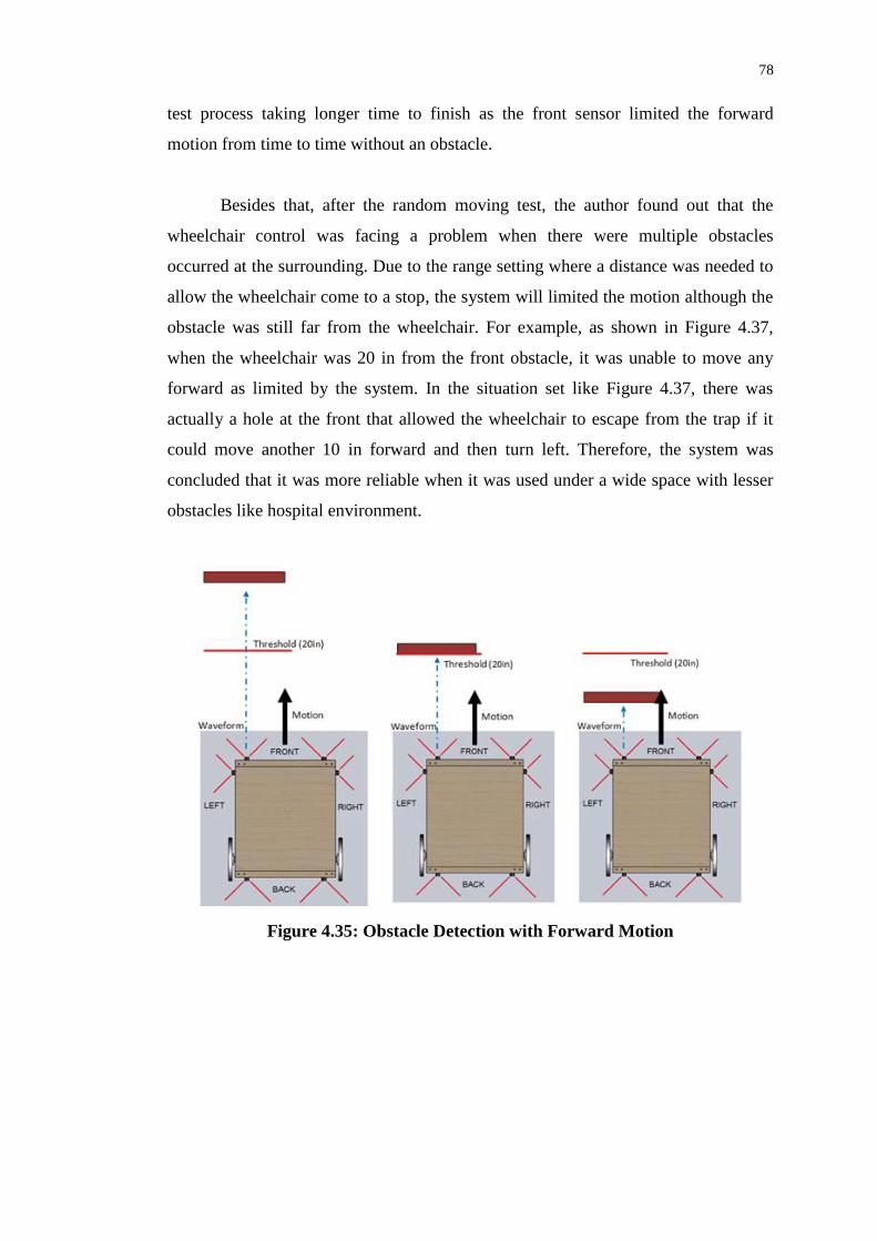
78
test process taking longer time to finish as the front sensor limited the forward
motion from time to time without an obstacle.
Besides that, after the random moving test, the author found out that the
wheelchair control was facing a problem when there were multiple obstacles
occurred at the surrounding. Due to the range setting where a distance was needed to
allow the wheelchair come to a stop, the system will limited the motion although the
obstacle was still far from the wheelchair. For example, as shown in Figure 4.37,
when the wheelchair was 20 in from the front obstacle, it was unable to move any
forward as limited by the system. In the situation set like Figure 4.37, there was
actually a hole at the front that allowed the wheelchair to escape from the trap if it
could move another 10 in forward and then turn left. Therefore, the system was
concluded that it was more reliable when it was used under a wide space with lesser
obstacles like hospital environment.
Figure 4.35: Obstacle Detection with Forward Motion
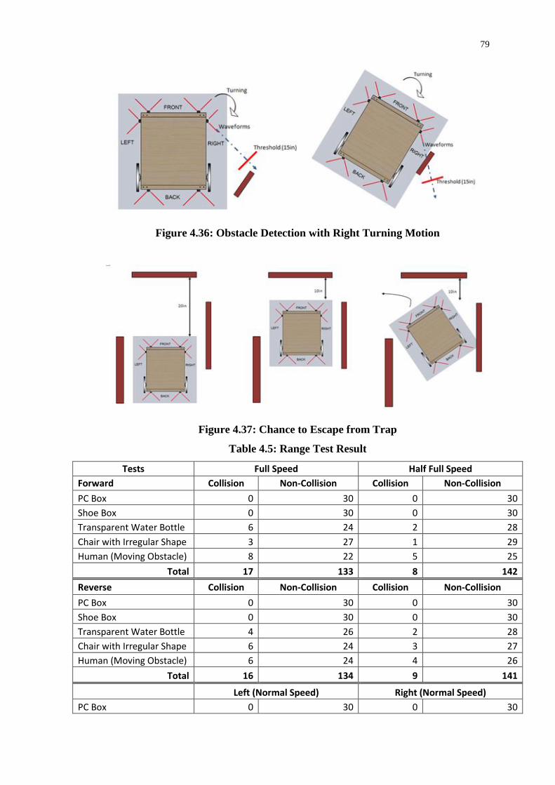
79
Figure 4.36: Obstacle Detection with Right Turning Motion
Figure 4.37: Chance to Escape from Trap
Table 4.5: Range Test Result
Tests Full Speed Half Full Speed
Forward Collision Non-Collision Collision Non-Collision
PC Box 0 30 0 30
Shoe Box 0 30 0 30
Transparent Water Bottle 6 24 2 28
Chair with Irregular Shape 3 27 1 29
Human (Moving Obstacle) 8 22 5 25
Total 17 133 8 142
Reverse Collision Non-Collision Collision Non-Collision
PC Box 0 30 0 30
Shoe Box 0 30 0 30
Transparent Water Bottle 4 26 2 28
Chair with Irregular Shape 6 24 3 27
Human (Moving Obstacle) 6 24 4 26
Total 16 134 9 141
Left (Normal Speed) Right (Normal Speed)
PC Box 0 30 0 30
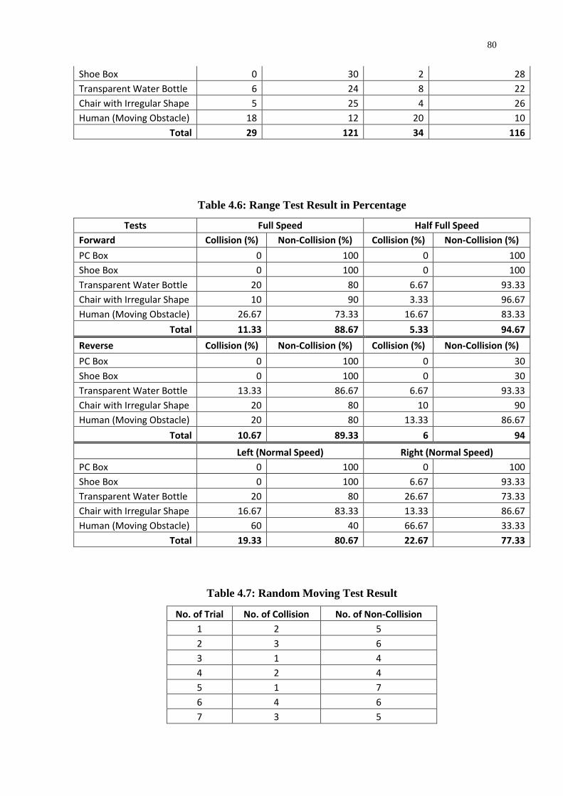
80
Shoe Box 0 30 2 28
Transparent Water Bottle 6 24 8 22
Chair with Irregular Shape 5 25 4 26
Human (Moving Obstacle) 18 12 20 10
Total 29 121 34 116
Table 4.6: Range Test Result in Percentage
Tests Full Speed Half Full Speed
Forward Collision (%) Non-Collision (%) Collision (%) Non-Collision (%)
PC Box 0 100 0 100
Shoe Box 0 100 0 100
Transparent Water Bottle 20 80 6.67 93.33
Chair with Irregular Shape 10 90 3.33 96.67
Human (Moving Obstacle) 26.67 73.33 16.67 83.33
Total 11.33 88.67 5.33 94.67
Reverse Collision (%) Non-Collision (%) Collision (%) Non-Collision (%)
PC Box 0 100 0 30
Shoe Box 0 100 0 30
Transparent Water Bottle 13.33 86.67 6.67 93.33
Chair with Irregular Shape 20 80 10 90
Human (Moving Obstacle) 20 80 13.33 86.67
Total 10.67 89.33 6 94
Left (Normal Speed) Right (Normal Speed)
PC Box 0 100 0 100
Shoe Box 0 100 6.67 93.33
Transparent Water Bottle 20 80 26.67 73.33
Chair with Irregular Shape 16.67 83.33 13.33 86.67
Human (Moving Obstacle) 60 40 66.67 33.33
Total 19.33 80.67 22.67 77.33
Table 4.7: Random Moving Test Result
No. of Trial No. of Collision No. of Non-Collision
1 2 5
2 3 6
3 1 4
4 2 4
5 1 7
6 4 6
7 3 5

81
8 2 5
9 5 4
10 3 6
11 2 5
12 5 5
13 1 8
14 4 7
15 2 5
16 3 6
17 6 6
18 5 4
19 4 6
20 3 4
21 1 4
22 2 7
23 4 6
24 5 4
25 3 5
26 2 6
27 2 5
28 1 4
29 3 5
30 4 6
Total 88 160
Figure 4.38: Graph of Random Moving Test

82
4.6.3 Automated Mode
Automated mode was used when the wheelchair was moved by itself without any
control from the user. Three systems, navigation system, obstacle detection system
and driving system were combined to form the whole system. Navigation system was
the one taking command from the user where the user had to set his current location
and then the destination. Once the user confirmed his choice, the navigation system
started to navigate to the destination with the wheelchair path prepared. During the
navigation, obstacle detection system was activated to detect if there was any
obstacle happened to block the path. Once an obstacle was detected, the system
would run its program and outputted the particular signals to the driving system to
avoid the obstacle. The wheelchair would back to the path after the obstacle had been
avoided. Once the wheelchair was back to the path, the navigation system was then
taken over the wheelchair control, while obstacle detection system was set back to
the detecting mode.
Again, trial and error method was used to determine the variables of the
coding like the threshold distance to detect an obstacle. After the coding was
completed, test was run for thirty times with the four obstacles prepared. Figure 4.39
showed the test setting where the setting was set on the navigation system testing
track and an obstacle was put at the front of the wheelchair. The wheelchair was
started by input the data of the current location and destination into the navigation
system. Once the obstacle prepared was detected by the system, the obstacle
detection system was taken over the wheelchair control by communicate with the
driving system. As set in the coding, the wheelchair leaned to the right side to avoid
the obstacle because the wheelchair path was decided to construct near to the left
wall. The result from tests was recorded in Table 4.8 and it was discussed in the next
section.

83
Figure 4.39: Automated System Test
4.6.3.1 Result and Discussion
The result for automated system test was presented in this section where Table 4.8
and Figure 4.40 were prepared. From Table 4.8, the test was perfect for PC box and
shoe box where there were zero collision for the thirty trials. Next, there was only
two collision happened when water bottle was the obstacle. With the result, the
success percentage was calculated to be 93.33% which was considered as a good
outcome. Unfortunately, the test becomes worse when the irregular shape chair was
used. The system failed to avoid the chair for twenty two times over thirty trials,
which gave a 26.67% of success rate only. The main factor causing such a result was
the irregular shape of the chair where there was no exact edge that presented as the
whole object edge. Due to its hollow design of the chair, the system was confuse on
determine front edge and end edge of the obstacle. Therefore, the system was failed
to avoid such an obstacle.
Table 4.8: Automated System Test Result
Obstacles Collision Non-Collision
PC Box 0 30
Shoe Box 0 30
Transparent Water Bottle 2 28
Chair with Irregular Shape 22 8
Total 24 96

84
Figure 4.40: Graph of Automated System Test
During earlier stage, instead of using edge detection concept only, the author
was combining edge detection and wall following concepts to construct the system.
The wall following was applied after the left sensor detected the front edge of the
obstacle. The system would then follow the obstacle boundary with the wall
following concept until it reached the end edge of the obstacle. Once the end edge
was detected by the left sensor, the wheelchair was concluded that it had pass by the
obstacle, and the wheelchair was started to move back to the wheelchair path. The
algorithm for the previous design was as shown as below, while the flowchart was
showed in Figure 4.41.
1. Detect obstacle bloking the front path.
2. Slow down the speed and start to steer to the right.
a. Front sensor detect obstacle edge. Go to step 3.
b. If not. Repeat with step 2.
3. Steer another short period to the right.
4. Move forward with slightly to the left steer.
a. Front sensor detect obstacle. Go to step 3.
b. If no. Go to step 5.
5. Move along obstacle boundary with left sensor.
a. Left sensor detect obstacle edge. Go to step 6.
b. If no. Repeat step 5.
6. Move forward with another short period.
7. Move forward with slightly left steering.

85
a. Detect line path (navigation system). Go to step 8.
b. If no. Repeat step 7.
8. Navigation system takes over the control.

86
Figure 4.41: Previous Automated Mode Flow Chart

87
Unfortunately, the system design failed to achieve the objectives. This was
because the obstacles prepared were not big enough for the wall following to take
part. Instead of finding a larger obstacle, the author concluded that it was impossible
for a large obstacle blocking the wheelchair path in a hospital. This was because the
path was specially constructed for the wheelchair and large object like furniture will
never put on the path. Therefore, the coding was modified to take out the wall
following concept and the outcome was as shown in result mentions previously.
Besides that, the surrounding condition for the system to avoid the obstacle
must clear from other obstacle. The system was build to avoid only one obstacle in a
time. If there was another obstacle tended to occur in the surrounding, the wheelchair
may collide with it. Further improvement on the automated system was needed and
was discussed in recommendation section.

88
CHAPTER 5
5 CONCLUSION AND RECOMMENDATIONS
5.1 Conclusion
The result showed in this project was acceptable and satisfied. It did achieve the
objectives of the project to a certain degree. I would like to conclude that semi-
automated mode achieved its objective in the sense that, it did help the wheelchair
preventing collision with the obstacle when the user was controlling. The system cut
off the particular motion control instead of giving warning to the user to stop the
wheelchair. Deceleration was provided instead of sudden stop to improve the
comfortable of the user. On the other hand, automated system was also concluded
that it did achieve the objective with the condition that there was only one obstacle
occurred in a time and the obstacle must has clear edges. Further study as mentioned
in recommendation section shall include in the project to improve the system.
5.2 Recommendations
Although the system was success to a certain degree, it was still can improve to make
the system perfect. A better fabrication of prototype may needs on future study so
that it is not the main factor affecting the result. Besides that, the automated system
has to improve so that it was able to deal with complex environment instead of one
obstacle in a time. For example, it may come to a stop first and check the
surrounding before take action in avoiding the obstacle that blocking the wheelchair

89
path. Next, the system may improve in the sense that the user was able to change the
mode of the system from time to time. For example, if the user is navigating from his
room to the cafeteria, he can change to semi-automated system so that he can control
the wheelchair to the toilet if needed.
90
REFERENCES
Bischoff, R., 1999. Advances in the Development of the Humanoid Service Robot
HERMES. In Second International Conference on Field and Service Robotics
(FSR’99). Pittsburgh, PA. Available at: http://www.rz.unibw-
muenchen.de/~161brai.
Borenstein, J. & Koren, Y., 1988. Obstacle avoidance with ultrasonic sensors. IEEE
Journal on Robotics and Automation, 4(2), pp.213–218. Available at:
http://ieeexplore.ieee.org/lpdocs/epic03/wrapper.htm?arnumber=2085
[Accessed December 14, 2012].
Fu, G., Menciassi, A. & Dario, P., 2012. Development of a low-cost active 3D
triangulation laser scanner for indoor navigation of miniature mobile robots.
Robotics and Autonomous Systems. Available at:
http://linkinghub.elsevier.com/retrieve/pii/S0921889012000929 [Accessed July
26, 2012].
Gojić, M., Brezak, M. & Petrović, I., 2011. Embedded computer control system for
service mobile robots. In MIPRO, 2011 Proceedings of the 34th International
Convention. pp. 711–716.
Kamon, I. & Rivlin, E., 1995. Sensory based motion planning with global proofs. In
Proceedings 1995 IEEE/RSJ International Conference on Intelligent Robots
and Systems. Human Robot Interaction and Cooperative Robots. IEEE Comput.
Soc. Press, pp. 435–440. Available at:
http://ieeexplore.ieee.org/lpdocs/epic03/wrapper.htm?arnumber=526253
[Accessed August 27, 2012].
Kinsky, P., Quan, Z. & YiMing, R., 2011. Obstacle Avoidance Robot, Available at:
http://www.wpi.edu/Pubs/E-project/Available/E-project-082811-
171143/unrestricted/Final_Report.pdf.
Mazo, M., 2001. An integral system for assisted mobility [automated wheelchair].
IEEE Robotics & Automation Magazine, 8(1), pp.46–56. Available at:
http://ieeexplore.ieee.org/lpdocs/epic03/wrapper.htm?arnumber=924361
[Accessed August 18, 2012].
Premadi, A. et al., 2009. Application of PIC microcontroller for online monitoring
and fiber fault identification. In 2009 International Conference on Electrical
Engineering and Informatics. IEEE, pp. 463–467. Available at:

91
http://ieeexplore.ieee.org/lpdocs/epic03/wrapper.htm?arnumber=5254693
[Accessed September 6, 2012].
Seki, H. et al., 2008. Practical obstacle avoidance using potential field for a
nonholonmic mobile robot with rectangular body. 2008 IEEE International
Conference on Emerging Technologies and Factory Automation, pp.326–332.
Available at:
http://ieeexplore.ieee.org/lpdocs/epic03/wrapper.htm?arnumber=4638414.
Yang, D., Xia, J. & Xi’ang, L., 2010. The Research on Intelligent Mobile Robot’s
Avoiding Obstacle by Ultrasound. 2010 International Conference on Artificial
Intelligence and Computational Intelligence, pp.77–79. Available at:
http://ieeexplore.ieee.org/lpdocs/epic03/wrapper.htm?arnumber=5656592
[Accessed July 27, 2012].
Yi, J. et al., 2009. Intelligent Robot Obstacle Avoidance System Based on Fuzzy
Control. In 2009 First International Conference on Information Science and
Engineering. IEEE, pp. 3812–3815. Available at:
http://ieeexplore.ieee.org/lpdocs/epic03/wrapper.htm?arnumber=5454890
[Accessed October 4, 2013].
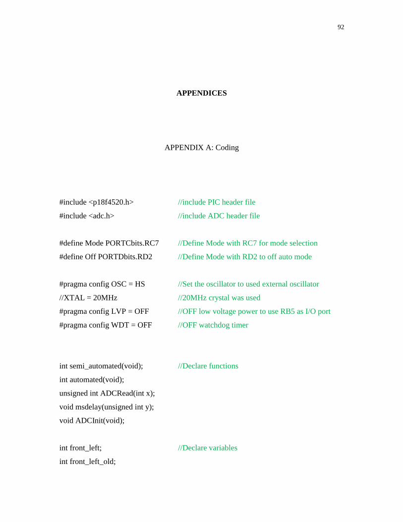
92
APPENDICES
APPENDIX A: Coding
#include <p18f4520.h> //include PIC header file
#include <adc.h> //include ADC header file
#define Mode PORTCbits.RC7 //Define Mode with RC7 for mode selection
#define Off PORTDbits.RD2 //Define Mode with RD2 to off auto mode
#pragma config OSC = HS //Set the oscillator to used external oscillator
//XTAL = 20MHz //20MHz crystal was used
#pragma config LVP = OFF //OFF low voltage power to use RB5 as I/O port
#pragma config WDT = OFF //OFF watchdog timer
int semi_automated(void); //Declare functions
int automated(void);
unsigned int ADCRead(int x);
void msdelay(unsigned int y);
void ADCInit(void);
int front_left; //Declare variables
int front_left_old;
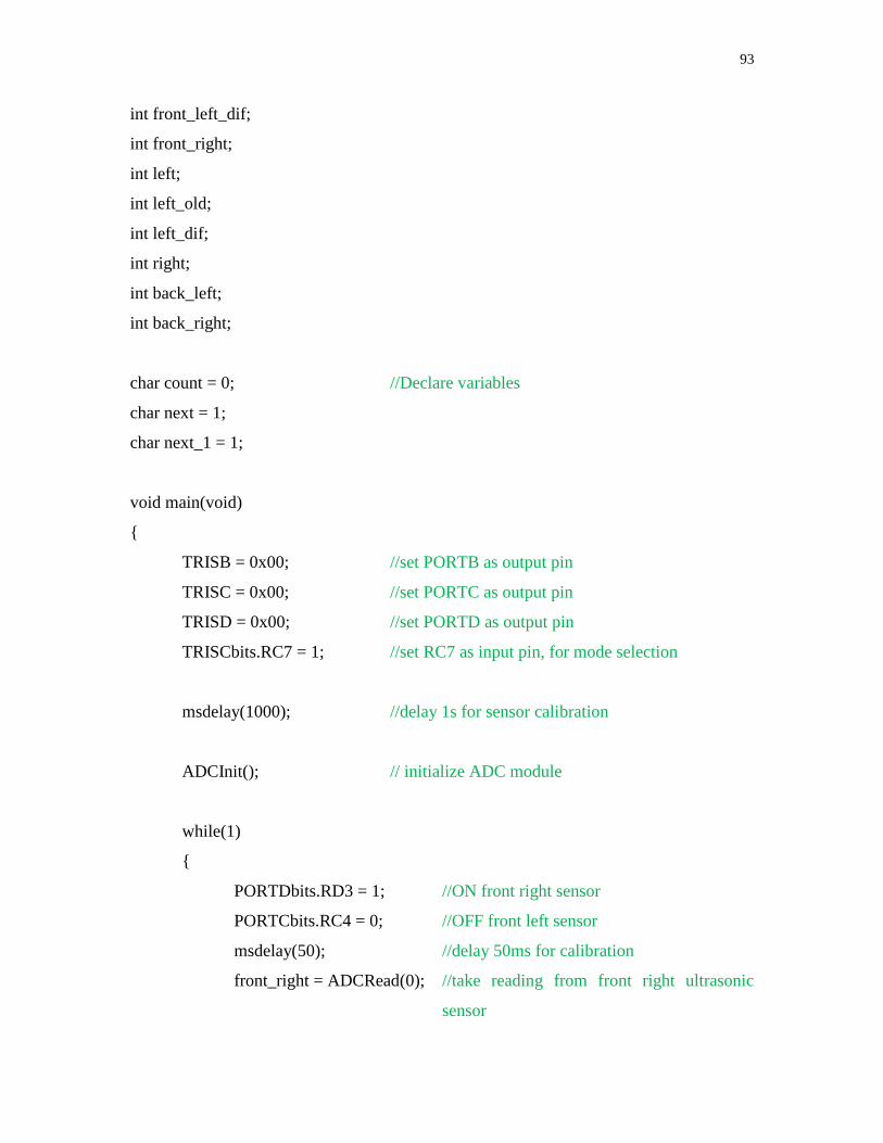
93
int front_left_dif;
int front_right;
int left;
int left_old;
int left_dif;
int right;
int back_left;
int back_right;
char count = 0; //Declare variables
char next = 1;
char next_1 = 1;
void main(void)
{
TRISB = 0x00; //set PORTB as output pin
TRISC = 0x00; //set PORTC as output pin
TRISD = 0x00; //set PORTD as output pin
TRISCbits.RC7 = 1; //set RC7 as input pin, for mode selection
msdelay(1000); //delay 1s for sensor calibration
ADCInit(); // initialize ADC module
while(1)
{
PORTDbits.RD3 = 1; //ON front right sensor
PORTCbits.RC4 = 0; //OFF front left sensor
msdelay(50); //delay 50ms for calibration
front_right = ADCRead(0); //take reading from front right ultrasonic
sensor

94
right = ADCRead(1); //take reading from right ultrasonic sensor
PORTDbits.RD3 = 0; //OFF front right sensor
PORTCbits.RC4 = 1; //ON front left sensor
msdelay(50); //delay 50ms for calibration
front_left = ADCRead(2); //take reading from front left ultrasonic
sensor
left = ADCRead(3); //Left ultrasonic sensor
PORTCbits.RC5 = 1; //ON back left sensor
PORTCbits.RC6 = 0; //OFF back right sensor
msdelay(50); //delay 50ms for calibration
back_left = ADCRead(4); //take reading from back left ultrasonic
sensor
PORTCbits.RC5 = 0; //OFF back left sensor
PORTCbits.RC6 = 1; //ON back right sensor
msdelay(50); //delay 50ms for calibration
back_right = ADCRead(5); //take reading from back right ultrasonic
sensor
if (Mode == 1) // automated mode
{
automated(); //call automated function
}
else if (Mode == 0) //semi-automated mode

95
{
semi_automated(); //call semi-automated function
}
}
}
int automated() // automated mode
{
PORTB = 0b00000000; //automated mode initialization
PORTD = 0b00000000;
front_left_dif = 0;
left_dif = 0;
//------Detect Obstacle------//
if (front_left <= 50 || front_right <= 50) // check obstacle? 25in distance (2bits/in)
{
PORTB = 0b00110000; //ON front left and front right indicator
PORTD = 0b00100000; //output lean right signal
//-----check whether front left sensor detect the front edge-----//
while (next)
{
PORTDbits.RD3 = 0; //OFF front right sensor
PORTCbits.RC4 = 1; //ON front left sensor
msdelay(50); //delay 50ms for calibration
front_left = ADCRead(2); //take reading from front left ultrasonic
sensor
front_left_old = front_left; //set front_left value into front_left_old
variable

96
msdelay(100); //delay 100ms
front_left = ADCRead(2); //take reading from front left ultrasonic
sensor
front_left_dif = front_left - front_left_old; //calculate the difference of
the front left sensor readings
if (front_left_dif >= 30) //if the difference larger than 15in (front edge
detected)
{
PORTB = 0b00100000; //ON front left indicator
PORTD = 0b10000000; //output forward signal
msdelay(2000); //delay for 2s
next = 0; //jump out of the while loop
}
}
}
//-----check whether left sensor detect the back edge-----//
while (next_1)
{
PORTB = 0b10000000; //ON left indicator
left = ADCRead(3); //take reading from left ultrasonic sensor
left_old = left; //set left value into left_old variable
msdelay(100); //delay 100ms
left = ADCRead(3); //take reading from left ultrasonic sensor
left_dif = left - left_old; //calculate the difference of the left sensor
readings
if (left_dif >= 30) //if the difference larger than 15in (end edge detected)
{

97
next_1 = 0; //jump out of the while loop
}
}
PORTB = 0b00000000; //OFF left indicator
msdelay(500); //blink left indicator with 500ms duration to show the stage
PORTB = 0b10000000; //ON left indicator
PORTD = 0b01000000; //output lean left signal
msdelay(4000); //delay 4s
PORTB = 0b00000000; //OFF front indicator
msdelay(500); //blink LED front indicator with 500ms duration to show stage
PORTB = 0b00110000; //ON front indicator
PORTD = 0b10000000; //output forward signal
while (end) //loop until navigation system take over
{
If (off == 1)
end = 1;
}
}
int semi_automated() //semi-automated mode
{
PORTD = 0; //semi automated mode initialization
if (front_left <= 40) // check obstacle? 20in distance (2bits/in)
{
PORTBbits.RB5 = 1; //ON front left indicator
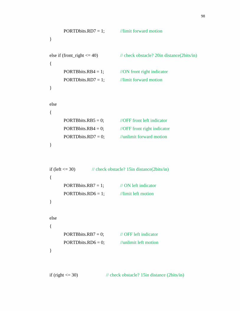
98
PORTDbits.RD7 = 1; //limit forward motion
}
else if (front_right <= 40) // check obstacle? 20in distance(2bits/in)
{
PORTBbits.RB4 = 1; //ON front right indicator
PORTDbits.RD7 = 1; //limit forward motion
}
else
{
PORTBbits.RB5 = 0; //OFF front left indicator
PORTBbits.RB4 = 0; //OFF front right indicator
PORTDbits.RD7 = 0; //unlimit forward motion
}
if (left <= 30) // check obstacle? 15in distance(2bits/in)
{
PORTBbits.RB7 = 1; // ON left indicator
PORTDbits.RD6 = 1; //limit left motion
}
else
{
PORTBbits.RB7 = 0; // OFF left indicator
PORTDbits.RD6 = 0; //unlimit left motion
}
if (right <= 30) // check obstacle? 15in distance (2bits/in)
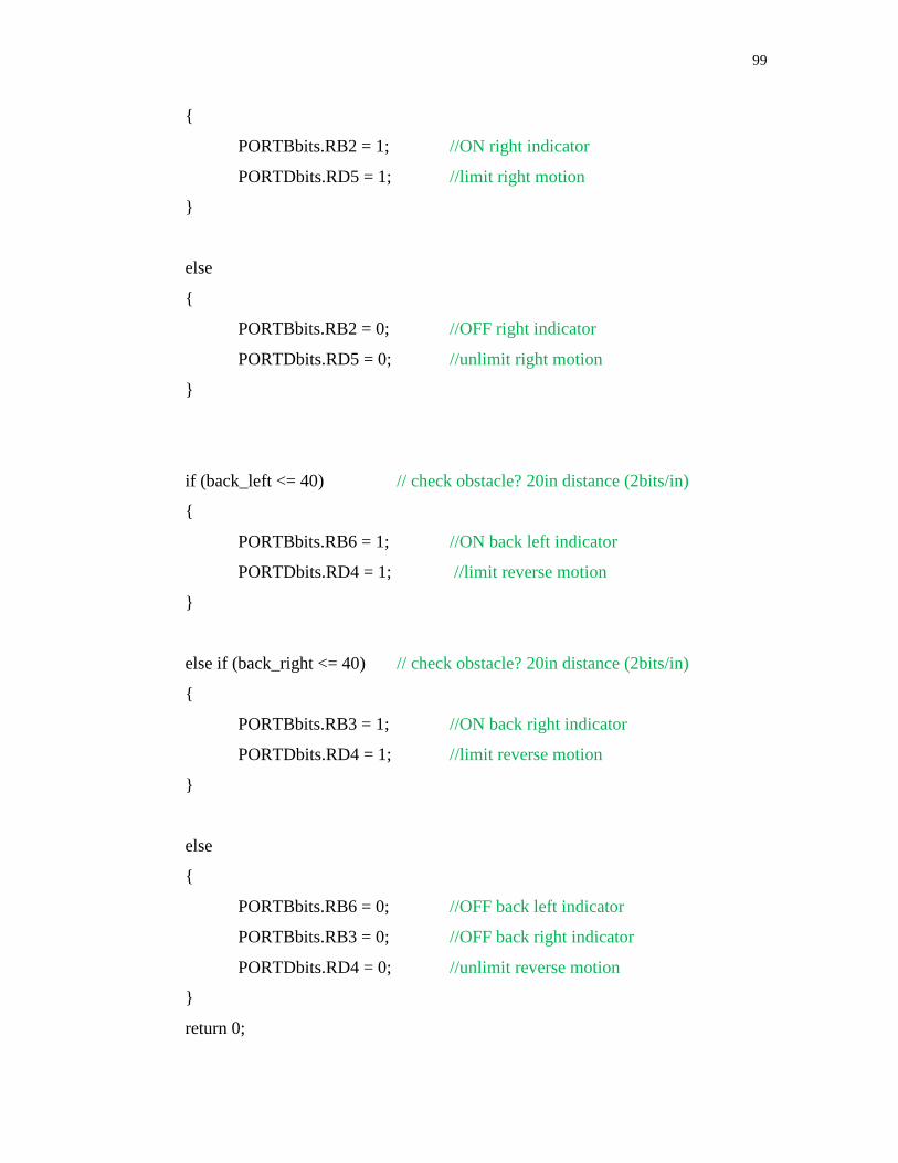
99
{
PORTBbits.RB2 = 1; //ON right indicator
PORTDbits.RD5 = 1; //limit right motion
}
else
{
PORTBbits.RB2 = 0; //OFF right indicator
PORTDbits.RD5 = 0; //unlimit right motion
}
if (back_left <= 40) // check obstacle? 20in distance (2bits/in)
{
PORTBbits.RB6 = 1; //ON back left indicator
PORTDbits.RD4 = 1; //limit reverse motion
}
else if (back_right <= 40) // check obstacle? 20in distance (2bits/in)
{
PORTBbits.RB3 = 1; //ON back right indicator
PORTDbits.RD4 = 1; //limit reverse motion
}
else
{
PORTBbits.RB6 = 0; //OFF back left indicator
PORTBbits.RB3 = 0; //OFF back right indicator
PORTDbits.RD4 = 0; //unlimit reverse motion
}
return 0;

100
}
}
void ADCInit(void)
{
ADCON1 = 0x08; //AN0,1,2,3,4,5 set to Analog, Vdd and Vss as voltage
reference
ADCON2 = 0x8a; //Right justified, 2Tad, Fosc/32
}
unsigned int ADCRead(int x)
{
ADCON0bits.CHS = x; //Select ADC channel
ADCON0bits.ADON = 1 ; //ON ADC
ADCON0bits.GO_DONE = 1; //Start ADC progress
while(ADCON0bits.GO_DONE); //wait for the conversion to finish
ADCON0bits.ADON = 0; //OFF ADC
return ADRES;
}
//-----provide 10ms per y-----//
void msdelay(unsigned int y)
{
unsigned int delval;
while(y)
{
delval = 380;
while(delval--);
y--;
}
}

101
APPENDIX B: Turnitin Report

102

103
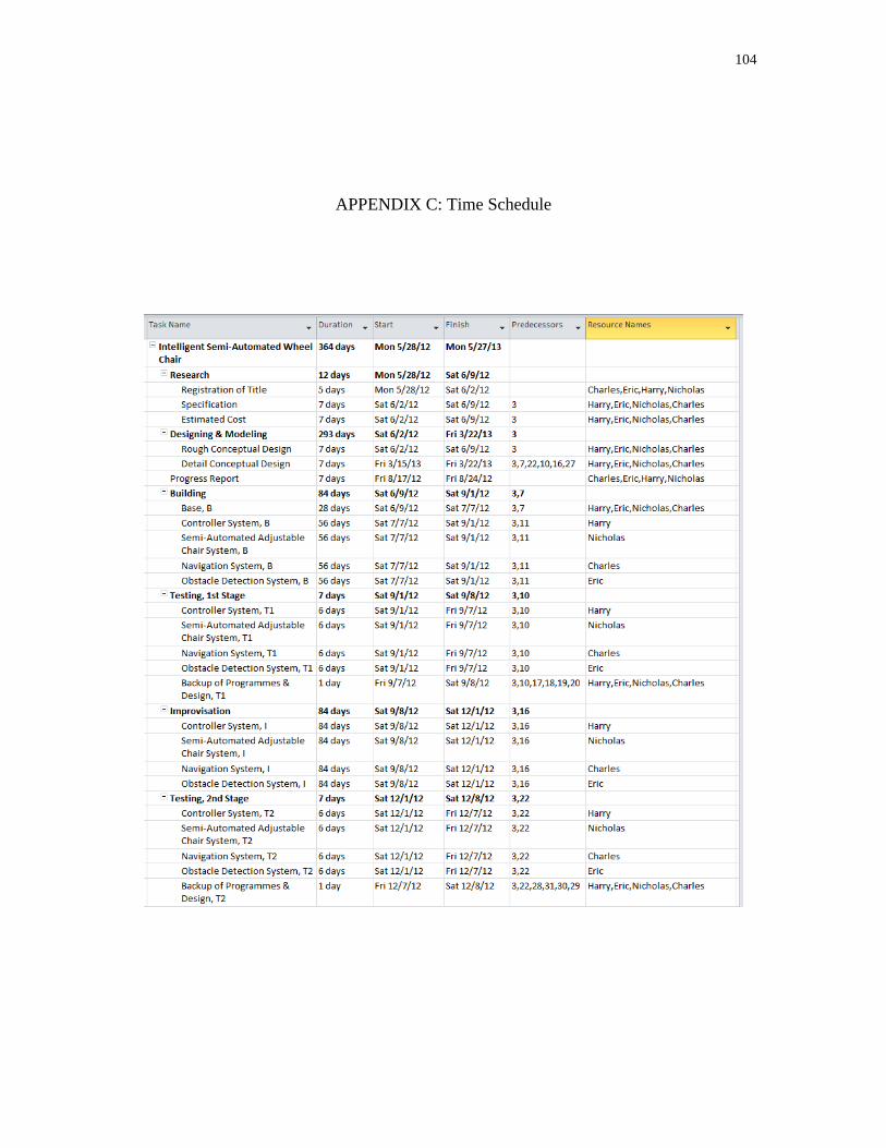
104
APPENDIX C: Time Schedule
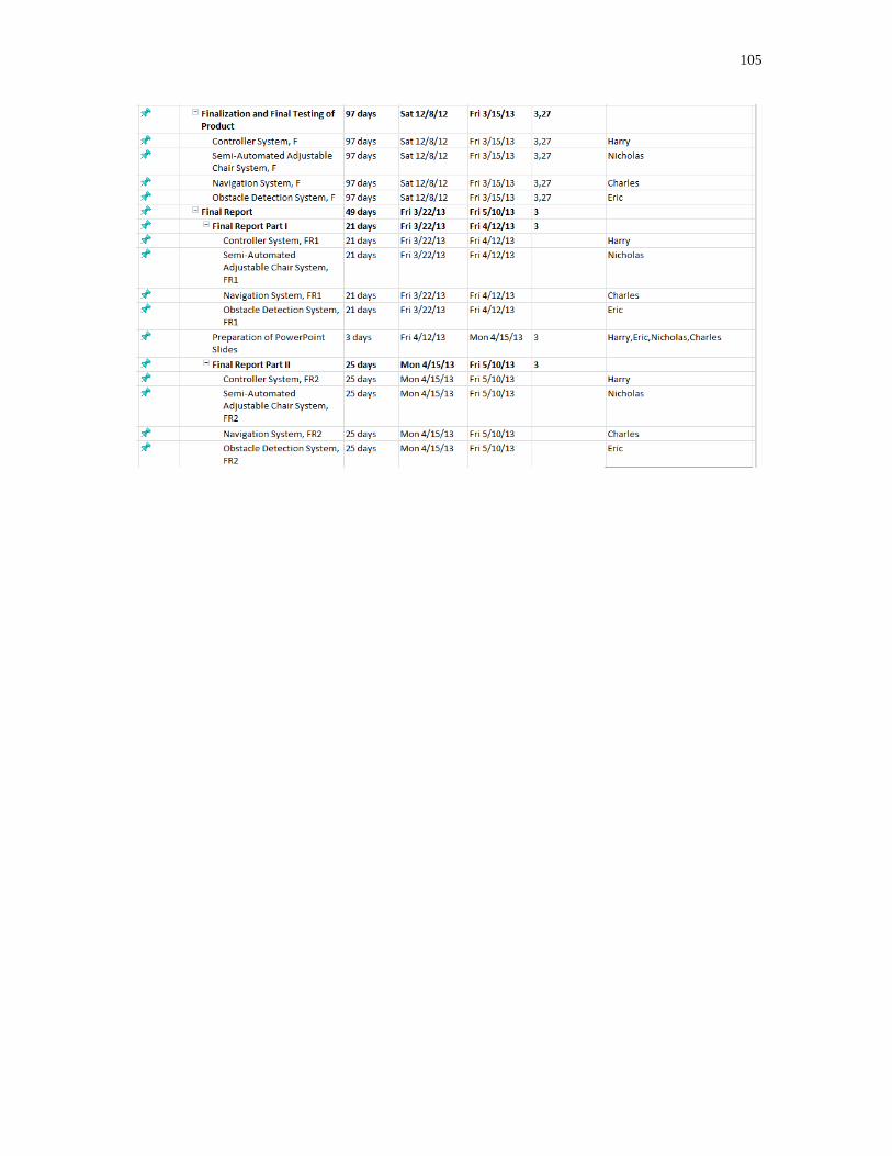
105

106
APPENDIX D: Gantt Chart

107
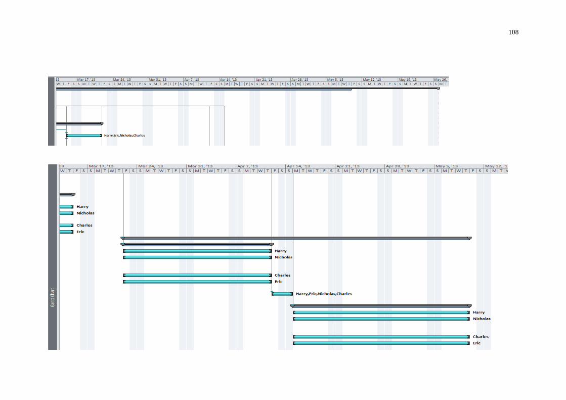
108