integrating remote-sensing and ground-based …...sandra brown (winrock international) george dyke...
TRANSCRIPT

Integrating remote-sensing and ground-based observations for estimation of emissions and removals of greenhouse gases in forests
Methods and Guidance from the Global Forest Observations Initiative
Version 1.0
January 2014

Citation
GFOI (2013) Integrating remote-sensing and ground-based observations for estimation of emissions and removals of greenhouse gases in forests: Methods and Guidance from the Global Forest Observations Initiative: Pub: Group on Earth Observations, Geneva, Switzerland, 2014.
ISBN 978-92-990047-4-6
Copyright and disclaimer
© 2013 Group on Earth Observations (GEO). The material may be freely distributed provided GEO is acknowledged.
The information contained in this report is believed to be correct at the date of publication. Neither the authors nor the publishers can accept any legal responsibility or liability for any errors or omissions.
GFOI Methods and Guidance
2

Acknowledgements
GFOI and GEO gratefully acknowledge the contributions to the MGD of the Advisory Group, the Lead Author Team, the Authors, Contributors and Reviewers listed below. GFOI and GEO are grateful for all inputs that helped to produce the MGD, from individuals and institutions, including support to the Lead Author team from the Australian Government Department of the Environment, the US SilvaCarbon Program and the UK Department for the Environment, Food and Rural Affairs.
Advisory Group and Author Team Membership
Advisory Group
Chair:
Jim Penman (Environment Institute, University College London)
Members:
Stephen Briggs (ESA)
Martin Herold (GOFC-GOLD and Wageningen University )
Thelma Krug (INPE, Brazil)
Alexander Lotsch (World Bank)
Kenneth MacDicken (FAO)
Douglas M. Muchoney (USGS, USA)
Orbita Roswintiarti (LAPAN, Indonesia)
Nalin Srivastava (IPCC)
Rob Waterworth (Australian National University)
Lead Author Team
Jim Penman (University College London)
Miriam Baltuck (CSIRO)
Carly Green (EAS)
Pontus Olofsson (Boston University and GOFC-GOLD)
John Raison (CSIRO)
Curtis Woodcock (Boston University and GOFC-Gold)
Authors and Contributors
Pradeepa Bholanath (Guyana Forestry Commission)
Cris Brack (Australia National University)
Deborah Burgess (Ministry of the Environment, New Zealand)
Eduardo Cabrera (IDEAM, Colombia)
Peter Caccetta (CSIRO)
Simon Eggleston (GFOI Office)
Nikki Fitzgerald (Australian Government, Department of the Environment)
Giles Foody (Nottingham University)
Basanta Raj Gautam (Arbonaut)
Shree Krishna Gautam (Department of Forestry Research and Survey, Nepal)
Alex Held (CSIRO)
Martin Herold (GOFC-GOLD and Wageningen University)
GFOI Methods and Guidance
3
Dirk Hoekman (Wageningen University)
Inge Jonckheere (FAO)
Leif Kastdalen (Norwegian Space Centre)
Pem Narayan Kandel (Department of Forest Research and Survey, Nepal)
Josef Kellndorfer (Woods Hole Research Center
Erik Lindquist (FAO)
Alexander Lotsch (World Bank)
Kim Lowell (University of Melbourne)
Richard Lucas (University of New South Wales)
Ronald McRoberts (US Forest Service)
Tony Milne (University of New South Wales)
Anthea Mitchell (University of New South Wales)
Brice Mora (GOFC-GOLD Land Cover Office)
Douglas M. Muchoney (US Geological Survey)
Erik Naesset (Norwegian University of Life Sciences)
Keryn Paul (CSIRO)
Shaun Quegan (University of Sheffield)
Ake Rosenqvist (soloEO)
Maria Sanz Sanchez (FAO)
Stephen Stehman (State University of New York)
Rob Waterworth (Australian National University)
Pete Watt Indufor (Asia-Pacific)
Mette Løyche Wilkie (FAO)
Sylvia Wilson (US Geological Survey)
Mike Wulder (Canadian Forest Service)
Reviewers
Heiko Balzter (University of Leicester)
Stephen Briggs (European Space Agency)
Sandra Brown (Winrock International)
George Dyke (Space Data Coordination Group)
Simon Eggleston (GFOI Secretariat)
Nagmeldin Elhassan (Higher Council for the Environment and Natural Resources, Sudan)
John Faundeen (USGS)
Giles Foody (Nottingham University)
Basanta Raj Gautam (Arbonaut)
Alan Grainger (University of Leeds )
Matieu Henry (FAO)
Mohamed Elgamri Ibrahim (College of Forestry and Range Science, Sudan University of Science and Technology)
Thelma Krug (INPE)
Ronald McRoberts (US Forest Service)
Brice Mora (GOFC-GOLD Land Cover Office)
Erik Naesset (Norwegian University of Life Sciences)
Dirk Nemitz (UNFCCC Secretariat)
Shaun Quegan (Sheffield University)
Ake Rosenqvist (soloEO)
Abdalla Gaafar Mohamed Siddig (Forests National Corporation, Sudan)
Stephen Stehman (State University of New York)
Nalin Srivastava (IPCC NGGIP TSU)
Tiffany Troxler (IPCC NGGIP TSU)
Stephen Ward (Space Data Coordination Group)
Rob Waterworth (Australian National University)
Pete Watt (Indufor Asia-Pacific)
Jenny Wong (UNFCCC Secretariat)
Hirata Yasumasa (FFPRI, Japan)
GFOI Methods and Guidance
4
TABLE OF CONTENTS
LIST OF ACRONYMS 12
SHORT GLOSSARY OF TERMS RELATED TO THE UNFCCC 16
PURPOSE AND SCOPE 20
1 Design Decisions 22
1.1 IPCC greenhouse gas inventory methodologies 22 1.2 Key category analysis 24 1.3 Definition of good practice 25 1.4 Design considerations for national forest monitoring system 26
1.4.1 Measuring, Reporting and Verifying 27 1.4.2 Reference Levels 27 1.4.3 Sub-national approaches 28 1.4.4 Forest definition 29 1.4.5 Use of existing information 31 1.4.6 Selection of appropriate approaches and tiers 33
1.5 Cost effectiveness 34
2 Estimating Emissions and Removals 36
2.1 Stock change and gain-loss methods 36 2.1.1 Stock change 36 2.1.2 Gain-loss 37
2.2 Methods for selected forest activities 40 2.2.1 Deforestation 40 2.2.2 Forest degradation 47 2.2.3 Sustainable management of forests, enhancement of C
stocks (within an existing forest), and conservation of C stocks 52
2.2.4 Estimation of emissions and removals for sustainable management of forests, enhancement of carbon stocks (within an existing forest), and conservation of carbon stocks 52
2.2.5 Enhancement of forest carbon stocks (afforestation of land not previously forest, reforestation of land previously converted from forest to another land use) 54
2.2.6 Estimation of emissions from enhancement of forest carbon stocks (afforestation of land not previously forest, reforestation of land previously converted from forest to another land use) 54
2.2.7 Conversion of natural forest 55
GFOI Methods and Guidance
5

3 Data Provision for Estimating Emissions and Removals 56
3.1 Activity data requirements 56 3.2 Remote sensing data sources 57
3.2.1 Coarse resolution optical data 58 3.2.2 Medium resolution optical data 58 3.2.3 High resolution optical data 60 3.2.4 Synthetic aperture radar 60 3.2.5 LiDAR 62
3.3 Pre-processing of satellite data 62 3.3.1 Pre-processing of optical satellite images 63 3.3.2 Pre-processing of SAR satellite images 64
3.4 Map products estimated from remote sensing 65 3.5 Methods for mapping activity data 69
3.5.1 Maps of forest/Non-forest, Land Use, or Forest Stratification 69
3.5.2 Maps of change 71 3.5.3 Maps of forest degradation 72
3.6 Guiding principles for remote sensing data sources and methods 73
3.7 Area, uncertainties and statistical inference for activity data 77 3.8 Collection of ground observations and the derivation of
emissions removal factors 84 3.9 Generic advice on use of ground observations to estimate
change in carbon pools and non-CO2 GHG emissions 85 3.9.1 Biomass 85 3.9.2 Dead wood and litter pools 90 3.9.3 Change in soil carbon stocks 90 3.9.4 Non-CO2 GHG emissions 91
4 Overall Uncertainties 94
4.1 Component uncertainties 94 4.1.1 Combining uncertainties 94
5 Reporting Requirements 97
6 References 99
Annex A Extended summary of IPCC guidance 107 Annex B Remote sensing data anticipated to be available
through GFOI arrangement with the CEOS Space Data Coordination Group 120
Annex C Tier 3 Methods 124 Annex D Sampling 132 Annex E Choice and use of emission and removal factors for
each REDD+ activity 136 Annex F Brief Review of the Potential for Direct Estimation of
Biomass by Remote Sensing 143 Annex G Developing and using allometric models to estimate
biomass 149 Annex H Financial Considerations 157
GFOI Methods and Guidance
6

Figures
Figure 1- Document Outline 11
Figure 2: Summary of key factors relevant to system design, and the selection of Tier and
Approach used for GHG estimation. 33
Figure 3: Decision Tree to guide selection of the method for estimating CO2 emissions and
removals depending on whether a country has an existing NFI. Note that generally
an NFI will only support estimation of change in biomass C pools, and not other C
pools. 39
Figure 4: Process Flow for Estimating Deforestation and Degradation Emissions 45
Tables
Table 1: Potential conversions contributing to deforestation and sections of the IPCC
Guidance relevant to estimating emissions associated with them 42
Table 2: Terms used in Equation 1 50
Table 3: Sources of emission/removal Factors of organic soils 51
Table 3: Terms used in Equation 2 53
Table 4: Major Activity Data Requirements for REDD+ Activities 56
Table 5: Recommended forest map products consistent with the methods outlined in Section
2.2 and Section 2.3.1 66
Table 6: Summary of types of remote sensing data and their perceived operational status in
estimating REDD+ activities (see Box 7 for Map Product Definitions) 67
Table 7: Example 1 – Error matrix of sample counts 79
Table 8: Example 1 – The error matrix of estimated area proportions 80
Table 9: Example 1 - Estimates and confidence intervals 81
Table 10: Example 2 - Regional estimates of deforestation area 83
GFOI Methods and Guidance
7

EXECUTIVE SUMMARY
The Global Forest Observations Initiative
The Global Forest Observations Initiative (GFOI) was established1 by the Group on Earth Observations in 2011, to assist countries to produce reliable, consistent and comparable reports on change in forest cover and forest use and associated anthropogenic greenhouse gas emissions or removals.
The Initiative will:
a) Work with the Committee on Earth Observing Satellites 2 to facilitate long-term provision of satellite earth observation data to countries. The Committee has established the Space Data Coordination Group specifically to address remote sensing requirements of GFOI.
b) Provide methodological advice on the use of remotely sensed data together with ground-based observations to estimate and report greenhouse gas emissions and removals associated with forests in a manner consistent with the greenhouse gas inventory guidance from Intergovernmental Panel on Climate Change (IPCC). This is required by decisions by the United Nations Framework Convention on Climate Change for voluntary implementation of REDD+ activities.
c) Identify research and development3 needed to improve data utility and accuracy of national forest monitoring systems that serve the greenhouse gas reporting requirements of the United Nations Framework Convention on Climate Change, as well as supporting broader environmental monitoring needs.
d) Help countries develop capacity to utilise earth observation data in national forest monitoring systems for reporting greenhouse gas emissions and removals. The GFOI capacity building effort complements readiness activities including those of the UN-REDD4 initiative and the World Bank Forest Carbon Partnership Facility.
The purpose of the Methods and Guidance Document is to provide methodological advice identified in point b), linked to the data made available via the Space Data Coordination Group referred to in point a).
Methodological advice and assistance with data access provided by the GFOI is potentially of interest to all countries wishing to make use of remotely sensed and ground-based data for forest monitoring and reporting. The initial focus is on reduced emissions from deforestation, forest degradation and associated activities, called REDD+5 in the climate negotiations.
1 GFOI builds on the work of the earlier Forest Carbon Tracking (FCT) programme, established by GEO in 2008 to demonstrate that international cooperation can provide data and information useful for national forest monitoring and reporting. 2 Established in 1984, CEOS coordinates civil space-borne observations of the Earth. See http://www.ceos.org/ 3 The GFOI Research and Development document is available from www.gfoi.org 4 United Nations collaborative initiative on Reducing Emissions from Deforestation and forest Degradation. 5 The REDD+ activities as listed in the Cancun Agreements (UNFCCC Decision 1/CP.16 para 70) are:
(a) Reducing emissions from deforestation; (b) Reducing emissions from forest degradation; (c) Conservation of forest carbon stocks; (d) Sustainable management of forests; (e) Enhancement of forest carbon stocks.
GFOI Methods and Guidance
8

The intended users of the Methods and Guidance Document are:
1. Technical negotiators working in the United Nations Framework Convention on Climate Change, who may be interested to see how REDD+ activities can be described and linked to the greenhouse gas methodology of the IPCC, as required by decisions of the Conference of Parties.
2. Those responsible for design decisions in implementing national forest monitoring systems.
3. Experts responsible for making the emissions and removals estimates.
The level of technical detail increases progressively through the Methods and Guidance Document. User groups 1 and 2 will probably be more interested in the earlier chapters, whereas the whole document will be relevant to user group 3. User group 1 is by definition based in-country; user groups 2 and 3 may be from countries or in organisations and initiatives working with countries, such as UN-REDD and the World Bank Forest Carbon Partnership Facility, and bilateral and multilateral arrangements.
The Methods and Guidance Document aims to increase mutual understanding between these user groups, and with the relevant science, technical and policy communities, to guide the collection of relevant forestry data, and to assist sharing of data and experiences. It aims to complement the guidance from the IPCC, the approach taken by the UN-REDD Programme6 and the GOFC-GOLD Sourcebook7, and has been produced in cooperation with these initiatives.
The Methods and Guidance Document complements the guidance from the IPCC by providing advice that takes account of the accumulated experience on the joint use of remote sensing and ground-based data, and is specific to REDD+ activities as set out in the Cancun agreements. Although guidance from the IPCC does treat deforestation in the Kyoto Protocol context8, in general it does not describe methodologies specific to REDD+ activities, as these were not specified until after the IPCC guidance and guidelines were written. The Methods and Guidance Document cross-references the IPCC guidance but does not repeat it. The word ‘guidance’ is used to refer to guidance from the IPCC; the Methods and Guidance Document uses ‘advice’ to mean new material that is complementary to IPCC guidance.
The Methods and Guidance Document recognizes the importance of national circumstances in determining the optimal mix of remote sensing and ground-based observations in the development of GHG inventories. National circumstances include current and future availability of technical expertise and institutional capacity to acquire and process data; the community, land-tenure, stakeholder, legal and administrative arrangements associated with
6 See National Forest Monitoring Systems: Monitoring and Measurement, Reporting and Verification (M & MRV) in the context of REDD+ Activities: http://www.un-redd.org/PolicyBoard2/9thPolicyBoard/tabid/106647
7 The November 2012 version of GOFC-GOLD sourcebook (used here) can be downloaded from http://www.gofcgold.wur.nl/redd/sourcebook/GOFC-GOLD_Sourcebook.pdf
8 See GPG2003 Section 4.2.6
GFOI Methods and Guidance
9

forestry and other land uses; the existence or otherwise of a forest inventory or other historical statistical data on land use; data accessibility, and issues such cloud cover, which can restrict the use of optical remote sensing methods, or terrain which makes access for taking ground measurements difficult.
Besides supporting the requirements to produce measurable, reportable and verifiable emissions and removals associated with REDD+, the Methods and Guidance Document should be relevant to countries for:
• estimating emissions and removals from the broader Land Use, Land-Use Change and Forestry sector;
• internal reporting and to assist with assessing the effects of domestic policies and actions;
• planning for other policy goals;
• providing information for country reports to the Global Forest Resource Assessment9 of the Food and Agriculture Organization of the United Nations.
The Methods and Guidance Document is presented in chapters that represent broadly the steps countries need to make in the development of estimates for reporting of Land Use, Land-Use Change and Forestry activities, including REDD+. The chapters cover:
1. Design decisions on scope and definitions of the system
2. Integration processes for estimating emissions and removals
3. Methods to collect, analyse and integrate input data
4. Reporting
The Methods and Guidance Document follows the development framework presented in figure 1 which is designed to guide the user through the document.
9 FAO has been monitoring the world's forests at 5 to 10 year intervals since 1946. Global Forest Resources Assessments (FRA) are now produced every five years, aiming to provide a consistent approach to describing the world’s forests and how they are changing. Assessments are based on two primary sources of data: Country Reports prepared by National Correspondents and remote sensing that is conducted by FAO together with national focal points and regional partners. For more information see www.fao.org/forestry/fra
GFOI Methods and Guidance
10

Figure 1- Document Outline
The grey arrows acknowledge that countries will continue to improve and adapt their input data and integration processes as technologies and capabilities evolve through continuous improvement process; for example by moving to more sophisticated (higher Tier) IPCC methods.
GFOI Methods and Guidance
11

LIST OF ACRONYMS
AD Activity Data
AGB Above Ground Biomass
ALOS Advanced Land Observing Satellite (Japanese series)
AMNF Total area of modified natural forest
APlantF Total area of planted forest
ASI Agenzia Spaziale Italiana (Italian Space Agency)
AVNIR Advanced Visible and Near Infrared Radiometer (Japanese series)
BUR Biennial Update Reports
C Carbon
CBERS China-Brazil Earth Resources Satellite series
CBMNF Biomass Carbon Density for modified natural forest
CBPF Biomass Carbon Density for primary forest
CBA Cost/Benefit Analysis
CO2 Carbon Dioxide
CO2degrad Annual CO2 emissions from degradation
CONAE Comisíon Nacional de Actividades Espaciales (Argentine Space Agency)
COP Conference of the (UNFCCC) Parties
CNES Centre Nationale d’études spatiales (French Space Agency)
CSA Canadian Space Agency
CSIRO Commonwealth Scientific and Industrial Research Organisation
CRESDA China Centre for Resources Satellite Data and Application
DCC Department of Climate Change
DEM Digital Elevation Model
DMC Disaster Monitoring Constellation
DFRS Department of Forest Resource and Survey (Nepal)
DLR Deutsches Zentrum für Luft- und Raumfahrt (German Aerospace Centre)
EROS Earth Resources Observation and Science Data Center
GFOI Methods and Guidance
12

EF Emission Factor
E/RF Emission and/or Removal Factor
ESA European Space Agency
EU European Union
FAO Food and Agriculture Organization of the United Nations
FCPF The World Bank’s Forest Carbon Partnership Facility
FRA Forest Resource Assessment
FTE Full Time Equivalent (Employee)
FullCAM Full Carbon Accounting Model
GFOI Global Forest Observations Initiative
GHG Greenhouse Gas or Greenhouse Gases
GIS Geographical Information System
GL Guidelines (IPCC 2006 Guidelines)
GLAS Geoscience Laser Altimeter System
GOFC-GOLD Global Observation of Forest Cover-Global Observation of Land Dynamics
GPG Good Practice Guidance (IPCC 2003 Good Practice Guidance)
IceSAT Cloud and land Elevation Satellite
INPE Instituto Nacional de Pesquisas Espaciais (Brazilian National Institute for Space
Studies)
IPCC Intergovernmental Panel on Climate Change
IRS Indian Remote Sensing satellite series
ISRO Indian Space Research Organization
JAXA Japanese Aerospace Exploration Agency
KOMPSAT Korea Multipurpose satellite series
KP Kyoto Protocol
L1G Landsat Level 1 Georectified
GFOI Methods and Guidance
13

L1T Landsat Level 1 Orthorectified
LAMP LIDAR-Assisted Multisource Program
LANDSAT Land Satellite (US Satellite series)
LEDAPS Landsat Ecosystem Disturbance Adaptive Processing System
LIDAR/LiDAR Light Detection and Ranging
LR Long-run or long term
LULUCF Land use, land-use change, and forestry
MGD Methods and Guidance Document
MODIS Moderate Resolution Imaging Spectroradiometer (US satellite series)
MNF Modified Natural Forest
MRV Measuring, Reporting, and Verification
NASA National Aeronautics and Space Administration
NASRDA Nigerian National Space Research and Development Agency
NCAS National Carbon Accounting System (Australia)
NFI National Forest Inventory
NFMS National Forest Monitoring System
NIS National Inventory System (Australia)
NMHC Non-methane hydrocarbons
PF Primary Forest
PlantF Planted Forest
RADARSAT SAR satellite series (Canada)
REDD+ Reducing Emissions from Deforestation, Reducing Emissions from Forest Degradation, Conservation of forest carbon stocks, Sustainable Management of Forests, and Enhancement of Forest Carbon Stocks
ROI Region of Interest
RF Removal Factor
RL Reference Level
SAOCOM Argentine Microwaves Observation Satellite
SAR Synthetic Aperture Radar
SPOT Satellite Pour l’Observation de la Terre (French satellite series)
GFOI Methods and Guidance
14
SRTM Shuttle Radar Topography Mission
TANDEM X TerraSAR-X add-on for Digital Elevation Measurement (Germany)
TerraSAR X SAR Earth Observation Satellite (Germany)
UN United Nations
UNFCCC United Nations Framework Convention on Climate Change
UN-REDD United Nations collaborative initiative on Reducing Emissions from Deforestation and forest Degradation (REDD). Participating UN Organizations are FAO, United Nations Development Programme (UNDP), United Nations Environment Programme
USD United States of America Dollar
USGS United States Geological Survey
WB World Bank
GFOI Methods and Guidance
15

SHORT GLOSSARY10 OF TERMS RELATED TO THE UNFCCC
Concept Meaning Notes Example reference (where applicable)
Activity data Data on the extent of human activity causing emissions and removals.
Activity data are often areas or changes in area.
GPG2003.
Emission or removal factors
GHG emissions or removals per unit of activity data.
GPG2003.
Forest Monitoring Functions of a national forest monitoring system to assist a country to meet measuring, reporting and verification requirements, or other goals.
Greenhouse gas inventory
Anthropogenic greenhouse gas estimates with national territorial coverage produced using IPCC methods in accordance with decisions taken at the UNFCCC Conference of the Parties (COP).
Covers energy, industrial processes and product use, agriculture, forests and other land use and waste. The COP has agreed to base REDD+ emissions and removals estimates on the latest IPCC methods agreed for the purpose.
COP decision 4/CP.15 requests the use of the most recent IPCC guidance and guidelines as adopted or encouraged by the COP; Annex III, part III of decision 2/CP17 identifies these as the Revised IPCC 1996 Guidelines and the IPCC Good Practice Guidance 2000 and 2003.
10 The Glossary provides explanations rather than formal definitions.
GFOI Methods and Guidance
16

Concept Meaning Notes Example reference (where applicable)
Ground based data Data gathered by measurements made in the field.
Measurement of gaseous concentrations could also be regarded as remotely sensed if the point of measurement is distant from what is being measured.
Measuring, Reporting and Verifying, also called Measurement, Reporting and Verification (MRV)
Procedures associated with the communication of all mitigation actions of developing countries.
Measuring is estimating the effect of the action, reporting is communication to the international community, and verifying is checking the estimation; procedures for all three are to be agreed by the UNFCCC.
Sometimes incorrectly called Monitoring, Reporting and Verifying.
Cancun Agreements (paras 61 to 64, COP decision 1/CP.16; decision -/CP19 11(Modalities for measuring, reporting and verifying).
National Forest Inventory (NFI)
A periodically updated sample-based system to provide information on the state of a country’s forest resources.
Historically not linked to greenhouse gas emissions, but where it exists, obviously a potential source of relevant data.
National Forest Inventories, Tomppo, E.; Gschwantner, Th.; Lawrence, M.; McRoberts, R.E. (Eds.), Springer 2010.
11 Decisions of the UNFCCC Conference of Parties are numbered but at the time of writing shortly after the Warsaw COP, numbers were yet to be assigned to the seven decisions on REDD+ reached at COP19. Hence they are all designated -/COP19 and need to be identified by their titles.
GFOI Methods and Guidance
17

Concept Meaning Notes Example reference (where applicable)
National Forest Monitoring System (NFMS)
The institutional arrangements in a country to monitor forests. NFMS will presumably include representation from responsible Ministries, indigenous peoples and local communities, forest industry representatives, and other stakeholders. In the REDD+ context, a system for monitoring and reporting on REDD+ activities, in accordance with guidance from the COP.
The COP has established that a NFMS should use a combination of remote-sensing and ground- based data, provide estimates that are transparent, consistent, as far as possible accurate, and that reduce uncertainties, taking into account national capabilities and capacities; and their results are available and suitable for review as agreed by the COP. NFMS may provide information on safeguards.
COP decisions 4/CP.15, 1/CP.16 and -/CP19 (Modalities for national forest monitoring systems).
REDD+ Reducing emissions from deforestation; Reducing emissions from forest degradation; Conservation of forest carbon stocks; Sustainable management of forests; Enhancement of forest carbon stocks.
COP decision 1/CP.16.
Remote Sensing Acquiring and using data from satellites or aircraft. Measurement of gaseous concentrations, could be regarded as remotely sensed if the point of measurement is distant from what is being measured.
GFOI Methods and Guidance
18

Concept Meaning Notes Example reference (where applicable)
Safeguards Undertakings to protect and develop social and environmental sustainability.
Covers consistency with national forest programmes and relevant international conventions and agreements; transparency and effectiveness of national forest governance; respect for the knowledge and rights of indigenous peoples and members of local communities; participation of relevant stakeholders, in particular indigenous peoples and local communities.
COP decisions 1/CP.16 and -/CP19 (covering the timing and frequency of presentation of summary information on safeguards).
GFOI Methods and Guidance
19

PURPOSE AND SCOPE
The purpose of the Global Forest Observations Initiative (GFOI) Methods and Guidance Document (MGD) is to provide countries with advice relevant to their development of national forest monitoring, and measuring, reporting and verifying (MRV) systems that use remotely sensed and ground-based data. The MGD provides information that can be customised to fit individual country circumstances and cope with both preferences and evolution in technology.
MGD advice helps fill a current gap in practical guidance on developing and implementing forest MRV systems, particularly concerning the integration of remotely sensed data with ground-based data to estimate emissions and removals of GHG from the land sector.
The MGD is relevant to all countries, but is particularly intended for policy and technical decision makers in developing countries, as well as their partners in international agencies, multilateral and bilateral programmes.
The MGD provides practical advice to help meet international reporting requirements by:
• describing requirements of the International Panel on Climate Change (IPCC) guidelines and United Nations Framework Convention on Climate Change (UNFCCC) decisions for estimating emissions and removals from the land sector.
• providing detailed advice on decision making and technical implementation, describing broad principles for the collection and use of data, thus remaining relevant even as technologies and methods evolve.
• illustrating how countries can apply the principles outlined in the document by using existing examples of national greenhouse gas inventories, and other operational systems such as those used for the early detection of deforestation.
The term guidance is used in the MGD where there is a cross-reference to IPCC and advice is applied where new, complementary material is provided by the MGD.
Recognizing the needs of end users the MGD:
• represents the process that countries need to work through to develop a system that meets national policy objectives
• incorporates decision trees and web links to help the user navigate and focus on the material/tools relevant to them
• is provided in both printed and web-based formats.
IPCC’s guidance recognizes the potential role of remote sensing (which can include aircraft borne sensors as well as images from satellites) in delivering GHG inventories, but does not go into detail apart from identifying techniques. The MGD complements the IPCC guidance by providing material that takes account of the accumulated experience on the joint use of remote sensing and ground-based data, and is specific to REDD+ activities. Although IPCC
GFOI Methods and Guidance
20

does treat deforestation in the KP context12, in general it does not describe methodologies specific to REDD+ activities, which were not specified until after the IPCC 2003 Guidance and 2006 Guidelines were written. The MGD provides advice for specific REDD+ activities.
The MGD recognizes the importance, both of MRV requirements and of national circumstances in determining the optimal mix of remote sensing and ground-based observations, and that these may evolve. National circumstances include the:
• existence or otherwise of a forest inventory or other historical statistical data on land use
• data accessibility and availability and meteorological issues e.g. cloud cover which can restrict the use of remote-sensing methods
• availability of technical expertise and institutional capacity to acquire and process data
• community, land-tenure, stakeholder, legal and administrative arrangements associated with forestry and other land uses.
12 See GPG2003 Section 4.2.6
GFOI Methods and Guidance
21
1 Design Decisions
Chapter 1 describes the greenhouse gas inventory methods produced by the IPCC including the concept of tiered methodologies, key category analysis and the definition of good practice. It discusses the functions that a national forest monitoring system may deliver, and issues surrounding forest definition. It addresses the use of existing information and issues of methodological choice. It deals with reference levels, the role of sub-national approaches and cost effectiveness.
1.1 IPCC greenhouse gas inventory methodologies
Since 1996, the IPCC has produced and published the guidance that countries have agreed to use in estimating GHG inventories for reporting to the UNFCCC and the Kyoto Protocol. These inventories cover all economic sectors including LULUCF. There is a well-established system under the UNFCCC and the Kyoto Protocol for reviewing inventories of developed countries, and this is the basis for assessing progress towards emissions reduction targets and commitments for these countries. For REDD+ activities, inventory estimates are likely to be a prerequisite for participation in results-based incentive schemes, both for estimating emissions or removals, and for establishing the reference levels and reference emission levels against which these will be assessed.
Following the 1996 Revised IPCC Guidelines for National Greenhouse Gas Inventories (IPCC, 1997), in 2000 the IPCC introduced its Good Practice Guidance (GPG2000) (IPCC, 2000). GPG2000 covers all sectors except LULUCF. In 2003, GPG was extended to GHG estimation for the LULUCF sector (GPG2003) (IPCC, 2003). The GPG2000 and GPG2003 work in conjunction with the 1996 Revised IPCC Guidelines. In 2006 IPCC published the 2006 IPCC Guidelines for National Greenhouse Gas Inventories (2006GL) (IPCC 2006) which combines LULUCF and agriculture into a single Agriculture, Forestry, and Other Land Uses (AFOLU) sector. The 2006GL use the same methodological framework as the GPG2000 and GPG2003.
In 2011 the UNFCCC decided that the Revised IPCC 1996 Guidelines in conjunction with the GPG2000 and GPG2003 should be used by developing countries for estimating and reporting anthropogenic emissions and removals13. Consequently, for REDD+, the inventory framework in which GFOI operates is defined by the GPG2003. The MGD will therefore cross-reference the GPG2003. Countries can presumably use scientific updates in the 2006GL within this framework, and so references to corresponding sections of 2006GL are also provided.
The GPG2003 provides methodologies to estimate changes in five carbon pools (above-ground biomass, below-ground biomass, dead wood, litter, and soil organic matter14) and non-CO2 GHG emissions for six categories of land use (Forest Land, Cropland, Grassland, Wetland, Settlements and Other Land), and for changes between land uses. Emissions and removals are estimated for land remaining in a category and for land converted between
13 See Decision 4/CP.15 and Part III of Annex III to the Durban Outcome of the work of the Ad Hoc Working
Group on Long-term Cooperative Action under the Convention (Decision 2/CP.17), developed countries will use the 2006GL
14 The GPG2003 also provides three alternative methods for dealing with harvested wood products.
GFOI Methods and Guidance
22

categories. Deforestation is estimated as the sum of emissions and removals associated with conversions from forest to other land uses. Forest degradation, conservation of forest carbon stocks, and sustainable management of forests are not identified by name in the GPG2003 (or in the 2006GL) but these can be estimated as the effect on emissions and removals of human interventions on land continuing to be used as forests15. Enhancement of forest carbon stocks may occur within existing forests and also include the effect of conversion from other land uses to forest. Chapter 2 of the MGD describes how to make these estimates, cross referencing the methods described by IPCC.
IPCC provides guidance on two generic calculation methods for estimating CO2 emissions and removals; the gain-loss method (which calculates emissions and/or removals directly) and the stock change method16 (which calculates emissions or removals from the difference in total carbon stocks at two points in time). Section 2.1 discusses considerations for selecting and applying these approaches.
Emissions of gases other than CO2 are estimated as the product of emission factors and activity data. IPCC methods also use auxiliary data, which consist of information that is useful in selecting or applying activity data and emission and removal factors, for example information on forest type and condition, management practice or disturbance history.
IPCC describes three approaches to providing activity data involving land area17. Approach 1 is not spatially explicit18 and simply uses net areas associated with managed land use. Approach 2 provides the matrix of changes between land uses. Approach 3 is fully spatially explicit. Remote sensing data are likely to be used to greatest advantage with Approaches 2 and 3. The three approaches are described and illustrated in section 2.3 of GPG2003, or section 3.3 of the 2006GL. IPCC methods require forest classification and associated stratification and the area of each stratum. IPCC methods are then applied at the level of the different carbon pools and the emissions and removals summed. IPCC methods do not necessarily require the existence of a formal national forest inventory (NFI).
IPCC describes methods at three levels of detail, called tiers. Box 1 summarizes the definition of Tiers, based on the description in the GPG2003. Tier 1 is also called the default method, and the IPCC guidelines aim to provide the information needed for any country to implement Tier 1, including emission and removal factors and guidance on how to acquire activity data. Tier 2 usually uses the same mathematical structure as Tier 1 but countries need to provide data specific to their national circumstances. This would typically require field work to estimate the values required if they do not exist. Tier 3 methods are generally more complex, normally involving modelling and higher resolution land use and land-use
15 In IPCC terms, forest land remaining forest land.
16 The methods are introduced in Section 3.1.4 of GPG2003, or Vol 4, Section 2.2.1 of the 2006GL. In the
2006GL the stock change method is called the stock-difference method. Chapter 2, volume 4 of 2006GL sets out the defining equations of the two methods.
17 See Chapter 2 of the 2003GPG, or Vol 4, Chapter 3 of the 2006GL
18 Spatially explicit means having a location that can be identified on the ground using geographical coordinates.
GFOI Methods and Guidance
23

change data. More detail on IPCC guidance can be found in Annex A, and Annex C provides examples of Tier 3 approaches being implemented by countries.
Spatial stratification by type or extent of human activities or type of forest should improve the quality of the results whatever the tier, for example, forests may be subdivided by using auxiliary data on ecosystem type, climate, elevation, disturbance history, and/or management practice. Box 4 provides a brief treatment of stratification.
A combination of tiers, most often Tier 1 and Tier 2 may be used. For national GHG reporting, any combination of Tiers and Approaches can be used. For REDD+ where spatially explicit information is needed to track activities and drivers, and to support estimation GHG emissions or removals, Approach 3 would be required.
Box 1: The IPCC Tier Concept
The IPCC has classified the methodological approaches in three different Tiers, according to the quantity of information required, and the degree of analytical complexity (IPCC, 2003, 2006).
Tier 1 employs the gain-loss method described in the IPCC Guidelines and the default emission factors and other parameters provided by the IPCC. There may be simplifying assumptions about some carbon pools. Tier 1 methodologies may be combined with spatially explicit activity data derived from remote sensing. The stock change method is not applicable at Tier 1 because of data requirements (GPG2003).
Tier 2 generally uses the same methodological approach as Tier 1 but applies emission factors and other parameters which are specific to the country. Country-specific emission factors and parameters are those more appropriate to the forests, climatic regions and land use systems in that country. More highly stratified activity data may be needed in Tier 2 to correspond with country-specific emission factors and parameters for specific regions and specialised land-use categories. Tiers 2 and 3 can also apply stock change methodologies that use plot data provided by NFIs.
At Tier 3, higher-order methods include models and can utilize plot data provided by NFIs tailored to address national circumstances. Properly implemented, these methods can provide estimates of greater certainty than lower tiers, and can have a closer link between biomass and soil carbon dynamics. Such systems may be GIS-based combinations of forest age, class/production systems with connections to soil modules, integrating several types of monitoring and data. Areas where a land-use change occurs are tracked over time. These systems may include a climate dependency, and provide estimates with inter-annual variability.
Progressing from Tier 1 to Tier 3 generally represents a reduction in the uncertainty of GHG estimates, though at a cost of an increase in the complexity of measurement processes and analyses. Lower Tier methods may be combined with higher Tiers for pools which are less significant. There is no need to progress through each Tier to reach Tier 3. In many circumstances it may be simpler and more cost-effective to transition from Tier 1 to 3 directly than produce a Tier 2 system that then needs to be replaced. Data collected for developing a Tier 3 system may be used to develop interim Tier 2 estimates.
1.2 Key category analysis
Key category analysis is the IPCC’s method for deciding which emissions or removals categories to prioritize in greenhouse gas inventory estimation, by using Tier 2 or Tier 3 methods. A category is key if, when categories are ordered by magnitude, it is one of the categories contributing to 95% of total national emissions or removals, or to 95% of the trend in national emissions or removals. Key category analysis including its application to the LULUCF sector, is described in section 5.4 of GPG 2003, corresponding to Volume 1, Chapter 4 of the 2006 Guidelines.
Key category analysis may need to be iterative; the initial ordering may need to be undertaken using Tier 1 methods, since it is not yet known which categories are key. REDD+ activities are not in general recognised categories in the IPCC inventory methodology, but in the case of deforestation, GPG2003 suggests adding up the conversions from forest to other land use that contribute to deforestation, and treating deforestation as key if the result is larger than the smallest category considered to be key using the recognised categories. This approach could obviously be extended to other REDD+ activities. IPCC also provides
GFOI Methods and Guidance
24

qualitative criteria for identifying key categories, one of which is that categories for which emissions are being reduced, or removals enhanced, should be treated as key. Since this qualitative criterion probably would apply in the case of REDD+ activities, they probably should be treated as key, although there has been no COP decision on this.
In applying key category analysis19 GPG 2003 asks whether particular sub-categories are significant. The subcategories are biomass, dead organic matter and soils. Significant subcategories (or pools) are those which contribute at least 25% to 30% of the emissions or removals in the category to which they belong. For subcategories which are not significant, countries may use Tier 1 methods if country specific data are not available. Identifying key sub-categories assists in the strategic allocation of additional resources to collect country specific data and in addition focuses efforts to reduce uncertainties related to these key sub-categories.
UNFCCC has decided20 that significant pools should not be omitted from forest reference emission levels or forest reference levels. The COP has not decided that the definition of significant in this case is the same as used by IPCC for key category analysis, but this is a possibility.
1.3 Definition of good practice
The concept of good practice underpins the GPG2003 and the 2006GL. Good practice is defined by IPCC21 as applying to inventories that contain neither over- nor under-estimates so far as can be judged, and in which uncertainties are reduced as far as is practicable. This definition has no pre-defined level of precision, but aims to maximize precision without introducing bias given the level of resources reasonably available for GHG inventory development. This level of resource is implicitly decided by the international inventory review process administered by the UNFCCC.
Good practice also covers cross-cutting issues relevant to GHG inventory development. These cover data collection including sampling strategies, uncertainty estimation, methodological choice based on identification of key categories (those which make greatest contributions to the absolute level of emissions and removals, and to the trend in emissions and removals), quality assurance and quality control (QA/QC), and time series consistency. QA/QC entails amongst other things validation (defined as internal self-consistency checks), and may include verification, defined as checks against independent, or at least independently-compiled, estimates. Remote sensing data may be useful for verification as well as for greenhouse gas inventory compilation, provided it is independent – that is, not already used for compiling the inventory.
19 As set out in section 3.1.6 of GPG2003 the decision trees provided by GPG2003 20 See the Annex to decision 12/CP.17, and paragraph 2, footnote 1 of -/CP19 (Modalities for national forest
monitoring systems)
21 See Section 1.3, 2003GPG, or Section 3 in the Overview in Vol 1 of the 2006GL
GFOI Methods and Guidance
25

Good practice entails the following general principles:
• Transparency (documentation sufficient for reviewers to assess the extent to which good practice requirements have been met)
• Completeness (that all relevant categories of emissions and removals are estimated and reported)
• Consistency (so that differences between years reflect differences in emissions or removals and are not artefacts of changes in methodology or data availability)
• Comparability (that inventory estimates can be compared between countries)
• Accuracy (delivered by the use of methods designed to produce neither under- nor over-estimates)
Use of remote sensing data may require particular attention to consistency, because satellites go out of commission and new ones enter into use, and ways of using the imagery evolve 22. This may affect time series of emissions estimates and the consistency with historical data which is necessary for establishing forest reference emission levels or forest reference levels. As described below, these are benchmarks for assessing the performance of REDD+ activities. Generic guidance for maintaining consistency is provided in GPG2003 and the 2006GL 23. Techniques should also be applied that minimise bias even if data sources do change over time (Box 8 and Section 3.6). Annex A provides an extended summary of IPCC guidance.
1.4 Design considerations for national forest monitoring system
COP19 24 (Warsaw 2013) reaffirmed, in line with decision 4/CP.15, that national forest monitoring systems (NFMS) should be guided by the most recent IPCC guidelines and guidance adopted or encouraged by the COP. NFMS should provide data and information that is transparent, consistent over time, and suitable for MRV of REDD+ activities, as well as consistent with decisions on nationally appropriate mitigation actions (NAMAs). They should build on existing systems, enable assessment of different forest types, including natural forest, as defined by a country, be flexible and allow for improvement. An NFMS should reflect, as appropriate, a phased approach. This begins with the development of national strategies or action plans, policies and measures, and capacity-building, is followed by their implementation and possibly further capacity-building, technology development and transfer and results-based demonstration activities, and evolves into results-based actions that should be fully measured, reported and verified25. COP19 acknowledged that Parties’ NFMS may provide appropriate information on how the safeguards set out in decision 1/CP.16 are addressed and respected. A separate decision at COP19 establishes that information on how the safeguards set out in 1/CP.16 are being addressed and respected should be provided via National Communications and on a voluntary basis via the REDD+
22 Annex B provides a list of relevant satellites available at the time of writing. 23 See Section 5.6 of the 2003 GPG (Time Series Consistency and Methodological Change) or Vol 1, Chapter 5
of the 2006 GL (Time Series Consistency) 24 Decision -/CP.19: Modalities for national forest monitoring systems. The summary is provided for the purposes
of the subsequent discussion in the MGD; please consult the full text of the decision for complete understanding of the REDD+ agreement reached in Warsaw.
25 See paragraphs 73 and 74 of decision 1/CP.16
GFOI Methods and Guidance
26

Web Platform on the UNFCCC web site26, once implementation of REDD+ activities has begun, and as a prerequisite to obtain and receive results-based payments.
Although not specified by the COP19 decision, the MGD assumes that, while building upon existing systems, an NFMS could engage a range of stakeholders including national authorities with responsibilities for forest land27, agencies responsible for collecting national data such as census information, agencies responsible for estimating forest related emissions and removals of greenhouse gases in the context of national greenhouse gas inventory estimates, and possibly stakeholder representatives including community representatives and the private sector. Depending upon national circumstances, the NFMS could be useful in delivering additional functions.
1.4.1 Measuring, Reporting and Verifying
COP19 agreed 28 that data and information used by Parties to estimate anthropogenic emissions and removals associated with REDD+ activities need to be transparent, consistent over time, and consistent with the forest reference emission levels (FRELs) and forest reference levels (FRLs), to be submitted by Parties under the provisions of Decision 12/CP.17. The COP 19 MRV decision encourages improvements of data and methodologies over time, whilst maintaining consistency with FRELs and FRLs. Parties seeking results-based payments for REDD+ activities are requested to provide a technical annex to the biennial update reports (BUR) including information on assessed FRELs and FRLs, the results of the implementation of the REDD+ activities expressed in tonnes of carbon dioxide equivalent per year, demonstration of consistency between results and FRELs and FRLs, information that allows reconstruction of results, and a description of the NFMS. The information contained in the technical annex will be analysed, the results published and areas for improvement identified. COP19 agreed that further verification modalities may be required in the context of market-based approaches.
1.4.2 Reference Levels
In 2011, decision 12/CP.17 established that FRELs and FRLs are benchmarks for assessing performance in implementing REDD+ activities, and that they should be set transparently, taking into account historical data, may be adjusted for national circumstances, and should maintain consistency with anthropogenic emissions and removals estimates as contained in each country’s greenhouse gas inventory. The same decision invited developing countries to submit reference levels on a voluntary basis. In 2013 the Warsaw COP decided that the FRELs and FRLs submitted under the provisions of decision 12/CP.17 shall be subject to technical assessment. An annex to the COP 19 decision provides information on the scope of the assessment; which includes consistency with emissions and removals estimates of REDD+ activities, how historical data have been used (including any modelling), transparency, completeness and accuracy, consistency of the forest definition with that used
26 See http://unfccc.int/redd 27 Such agencies could include those responsible for Forestry, Agriculture, and Environment. 28 Decision -/CP.19: Modalities for measuring, reporting and verifying.
GFOI Methods and Guidance
27

for other international reporting, inclusion of assumptions about future changes to domestic policies included in reference levels, pools and gases included and justification concerning why omitted pools and gases were deemed not significant, and updating of information which is contemplated by the stepwise approach already established in 12/CP.17.
COP19 recognised the importance of addressing drivers of deforestation and forest degradation, their complexity and their linkage to livelihoods, economic costs and domestic resources. Parties, relevant organisations and the private sector are encouraged to work together to address drivers of deforestation and forest degradation, and to share information including via the UNFCCC REDD+ Web Platform. From a technical perspective, gathering evidence to assess the relationships requires quantification of the effect of drivers on emissions and removals, examples of which include direct causes such as pressure from commercial or subsistence agriculture, commercial timber extraction, fuel-wood collection and charcoal production, conservation and sustainability policies and other policy drivers. Taking drivers into account may be useful in stratification and in ensuring consistency between historical data and reference levels.
1.4.3 Sub-national approaches
REDD+ in the context of UNFCCC aims at national level implementation; in other words emissions and removals are quantified in the context of national greenhouse gas inventories reported through the BURs, and performance measured against national reference levels (FRLs and FRELs). Implementation at the national level reduces concerns associated with project level engagement, especially the risk of leakage 29 . However, sub-national demonstration activities (those which do cover a significant area but not extend to full national areal coverage), are recognized as an interim step to national REDD+ implementation, including sub-national forest monitoring. According to the Cancun Agreements full implementation of results-based actions would require national forest monitoring systems. There are also some additional issues raised by sub-national engagement, for example there may be a need to assess leakage within a country, at state, province or project boundary. When establishing sub-national systems it is important to consider how the system will be included consistently within the final national system, and which components (in particular remote sensing) can readily be produced at the national level for use in sub-national estimates.
29 Leakage is the displacement of the forest activity outside the area monitored. National approaches help deal with leakage because the whole country is covered. Where project approaches simply monitor the project area the risk of missing emissions due to leakage is higher.
GFOI Methods and Guidance
28

1.4.4 Forest definition
A forest definition is needed to be able to determine whether deforestation or afforestation or reforestation has taken place, and to define the areas within which degradation and the other REDD+ activities may occur.
The IPCC 2003 GPG defines Forest Land as including all land with woody vegetation consistent with thresholds used to define forest land in the national GHG inventory, sub-divided into managed and unmanaged, and also by ecosystem type as specified in the IPCC Guidelines. It also includes systems with vegetation that currently fall below, but are expected to exceed, the threshold of the forest land category. The Forest Land definition in the 2006GL refers to threshold values. IPCC therefore anticipates that countries will have a forest definition with quantitative thresholds.
No single definition has been agreed under the UNFCCC for REDD+ purposes. Countries will often have an existing forest definition in place, and the COP has decided that, as part of the guidelines for submission of information on forest reference levels, Parties should provide the definition of forest used, and if there is a difference with the definition of forest used in the national greenhouse gas inventory or in reporting to other international organizations, an explanation of why and how the definition used in the construction of forest reference emission levels and/or forest reference levels was chosen30.
Countries that do not already have a forest definition may wish to note that for Kyoto Protocol (KP) purposes Forest …is a minimum area of land of 0.05–1.0 hectare with tree crown cover (or equivalent stocking level) of more than 10–30 per cent with trees with the potential to reach a minimum height of 2–5 metres at maturity. A forest may consist either of closed forest formations where trees of various storeys and undergrowth cover a high proportion of the ground or open forest. Young natural stands and all plantations which have yet to reach a crown density of 10–30 per cent or tree height of 2–5 metres are included under forest, as are areas normally forming part of the forest area which are temporarily unstocked as a result of human intervention such as harvesting or natural causes but which are expected to revert to forest31..
In developing an NFMS, countries will need to establish whether there is an existing forest definition, and if not to put one in place. Definitions can differ in ecosystem coverage, which can have a significant effect on the estimate of emissions or removals associated with REDD+ activities, and the allocation to activity (Box 2). Definitions should therefore be used consistently over time, and the definition used to establish the FRL or FREL should be the same as that used for subsequently for MRV.
30 See the Annex to decision 12/CP.17, Guidelines for submissions of information on reference levels
31 In the Forest Resource Assessment 2010 FAO defines Forest as Land spanning more than 0.5 hectares with trees higher than 5 meters and a canopy cover of more than 10 percent, or trees able to reach these thresholds in situ. It does not include land that is predominantly under agricultural or urban land use. The area threshold falls within the range in the KP definition and the height threshold is at the upper end of the KP range.
GFOI Methods and Guidance
29

Increasingly, the UNFCCC is emphasizing forest diversity and multifunctionality, and the difference between natural forests and plantations. The Cancun Agreements specify that REDD+ mitigation actions should not incentivize conversion of natural forests and the forest definition should therefore allow natural forests to be distinguished.
It is important that national forest definitions support reliable classification of land use and land use change and hence the estimate of major emissions or stock change. The ability to detect the transition between land classes using the national forest definition should be a consideration. For example the minimum area used in the forest definition can have implications for the spatial resolution of the imagery used to detect change. Additionally, scale, intensity and spatial distribution may affect the ability to track the identified drivers of change.
The IPCC definition requires forests to be subdivided into managed and unmanaged. This is because carbon stock changes and greenhouse gas emissions on unmanaged land are not reported under the IPCC Guidelines, although reporting is required when unmanaged land is subject to land use conversion32. The detailed definition of what is unmanaged may differ from country to country, but national definitions should be applied consistently over time otherwise there is risk that apparent changes in emissions will reflect differences in the way definitions are applied, rather than the effect of REDD+ activities.
National forest definitions selected and used by the NFMS should be documented, defendable, consistent over time and able to capture emissions and removals of the key activities.
Box 2: Exploring different forest definitions and their impact on developing REDD+ reference emission levels: A case study for Indonesia (Rominjin, E., et al., 2013).
A comparative study showed the effect in the case of Indonesia of applying three different forest definitions. The study estimated the total area of deforestation between 2000 and 2009 to be 4.9 million ha when using the FAO definition, 18% higher when using a definition focussed on natural forests and 27% higher when using the national definition.
The study found that it is important to have a separate class of forest plantation to capture the conversion from natural forest into forest plantation as this has large implications for estimation and allocation of emissions. In the analysis, conversion of natural forest into forest plantations was only detected as deforestation using the natural forest definition, but as degradation by the other two definitions.
The study noted that establishing plantations in natural forests can cause large CO2 emissions, especially on peat-lands. It is important that these CO2 emissions are captured, either as deforestation or as degradation, depending on the definition used. It was found important to harmonize forest definitions in a single country. The same forest definition should be used throughout the country and for different years for REDD+ monitoring, deforestation and degradation area estimates, and for estimates of drivers of deforestation and forest reference emission levels and forest reference levels.
32 GPG2003 Chapter 2, page 2.5
GFOI Methods and Guidance
30
1.4.5 Use of existing information
A requirement in the development of a forest monitoring system includes establishing knowledge gaps, identifying the information needed, and prioritizing tasks accordingly. Existing knowledge, with enhancements if needed, can be used to improve the speed and efficiency of the development of a forest monitoring system, if gaps can be filled without introducing significant bias. Establishing a comprehensive database of existing information, perhaps via the NFMS, will reveal what is available, and assist with setting priorities.
NFIs or other systematically established and measured plot systems are not required by IPCC guidance, but where they do exist they can be integrated into the forest monitoring system. Existing NFI (Box 3) or other plot data may be used in the stock change or gain- loss approaches (sections 2.1.1 & 2.1.2), though it may be necessary to establish additional plots (where the original plots under-represent some parts of the population) or to use auxiliary data in the case of a model-based approach. Annex D contains background on sampling, and on design-based and model-based approaches.
Plots not used in emissions or removals estimation may be useful for verification purposes. Allometric or other modelling will be required to estimate biomass and carbon from the tree and plot data, as it is unlikely that older forest inventories will have been designed to capture total biomass carbon directly (see section 2.1.1). Allometric or other models to convert forest inventory data into estimates of above- and below-ground biomass and carbon may already exist, and supplementary studies can fill gaps for other major species or forest types and environmental zones identified. Growth and yield trials, forest experiments and other quality data sources held by universities or other research agencies may be useful for the development or verification of models. The spatial, environmental or other limits of such models will need to be determined to ensure they are not applied outside their domain of relevance, as this may introduce bias. Any gaps, especially in the root-to-shoot or below ground allometrics could be filled through targeted new studies.
Effective application of sampling strategies and models often relies on stratification by climate (rainfall, temperature) or broad environmental conditions (altitude, topography, soil type), possibly integrated into bio-geo-climatic zones. Such data may also be used directly to develop growth indices (e.g. net primary productivity) or as input into growth models or for prediction of carbon allocation ratios. Networks of weather stations and historical records can be enhanced through spatial modelling approaches to develop climate surfaces for use as input into models or for more effective stratification.
Spatial data, including archived maps and GIS databases, may include coverage of forest types, disturbance history, age and condition. Remotely sensed data, including archives of such data, are a useful source of spatial information for stratification; improving identification of areas where there may be high potential for significant change in carbon stocks; and for identifying areas unrepresented by existing allometrics. Where national coverage is incomplete or inconsistent, for example due to administrative or tenure boundaries or use of differing methods for data collection, supplementary work by local experts may be a cost-effective way remedy.
GFOI Methods and Guidance
31

Although dynamics of soil carbon under a range of forest types and land use changes is often poorly understood, existing information that can be synthesised to create spatial coverage or emissions and removal factors on forest soil and changes in response to disturbance and management may be available from regional surveys and research studies. Expanding from a small and non-representative set of soil data to create adequate spatial coverage can be expensive given the variability of soil carbon and the expense of accurately measuring at each sample location. There are a number of process-based models that estimate soil parameters from physical and physiological principles. These models need extensive calibration using climatic and environmental data, but this may be less expensive than relying on sampling alone, and existing data sets may be used for calibration, if they correspond to the model variables and are sufficiently documented.
BOX 3: National Forest Inventories (NFIs)
National forest inventories (NFIs) exist in many countries to provide support for national level planning of forested lands and meet international data reporting commitments or agreements. Typically NFIs consist of a series of plots (or clusters of sub-plots) ranging from 0.02 ha to more than 1 ha in size established in a systematic fashion across the land defined as being of interest. Observations and measurements on these plots vary widely around the world but usually include data on tree and shrub species diversity; aspects of tree size (at least diameter at breast height, but also bole or tree height and condition) and general topography. Less commonly, observations or measurements will also include aspects of litter and dead material, site history, soil and canopy characteristics. When integrated with appropriate allometrics or other models, these NFI data provide estimates of forest population parameters – usually production or development related - at a precision relevant to national level planning.
When measurements on the plots are conducted at multiple points in time, annual change (and associated carbon change) can be calculated for each plot. The timing of plot re-measurements within an NFI varies from only a couple of years in fast growing environments to 5 or 10 years in slower growing environments, or environments that are more expensive to access and measure. Commonly, a proportion of all plots (a panel) is measured each year so that the entire system is measured over a 5 to 10 year period to smooth out the annual expense of measurement. Heikkinen et al. (2012) describe methods for making more precise estimates using panel (multi-dimensional) datab and data obtained using other NFI sampling designs.
As design-based sampling systems, these NFI estimates of totals, change and variance will be unbiased provided the probabilities of plot selection remain appropriate. Estimates of the total or variance for sub-sets of the original forest area are possible if sufficient plots can be grouped into domains or strata and all points within the domain have a probability greater than 0 that they could have been selected for inclusion in the original sample. The number of plots required depends on variability and precision required, and the need to detect events, such as deforestation. Selected or non-random increases or reductions in the forest land base would result in some land having zero probability of being included or alternatively that the sum of all the probabilities exceed 1 which will tend to violate design-based sampling principles and thus invalidate conclusions about unbiased estimates.
Where NFI data are (or can be) grouped according to strata being used for REDD+ estimation they are likely to be valuable sources of emission factor data. However since the land base relevant to forest carbon may well be different to the population originally sampled in the NFI, and land for deforestation or other REDD+ activities is unlikely to be randomly occurring across the landscape, population estimates of carbon totals or emission factors and variance from NFIs cannot be assumed to be unbiased. The best use of NFIs if this is not the case would be as one source of well measured and spatially located individual plot data over a wide range of environments that can be used for Remote Sensing training, calibration, verification or as inputs into double sampling or model-based sampling systems.
It is possible to maintain the design-based sampling approach for NFIs that have been established on a systematic pattern. The pattern could be expanded using the same system to include all the land relevant to the forest carbon inventory (e.g. to include forests on privately managed land or within land classified as Agricultural, urban or other where they meet the adopted definition of forest). The intensity or number of plots may also need to be increased to ensure there are sufficient plots within the domains where change (deforestation or degradation) is happening or likely to happen. However, unless there are other reasons for maintaining an independent NFI, such a simple expansion of a grid may be relatively costly compared to alternatives such as model-based sampling for given levels of precision.
Properly implemented, NFI-based methods satisfy Tier 3 requirements for the above-ground biomass pool as set out in the GPG2003: (i) primary focus on Forest Land remaining Forest Land, (ii) detailed use of NFI data, and (iii) use of models calibrated to national circumstances, and the unbiased statistical estimators used by NFIs satisfy the GPG requirement to neither over- nor under-estimate true change, so far as can be judged. Long-
GFOI Methods and Guidance
32

established NFIs are well-documented with respect to the validity and completeness of the data, assumptions, and models. Although new tropical NFIs do not have such long histories, and may face additional difficulties with placing plots in tropical countries due to access in natural forests, their methods and documentation can build on the historical NFI lessons learned with respect to sampling designs, field protocols, and statistical estimators. a Use of permanent plots increases precision of change detection – see GPG2003 section 5.3.3.3. If a permanent plot is deforested a new plot is established consistent with the NFI sampling scheme b In this context panel data means data from permanent plots sampled more frequently than the rotation period of the NFI. c FAO provides a basic discussion on the relationship between sample size and precision – see the National Forest Assessments Knowledge Reference at http://www.fao.org/forestry/13447/en/
1.4.6 Selection of appropriate approaches and tiers
The selection of the appropriate Tier and Approach to use for GHG estimation and for other purposes depends on country circumstances. A summary of the key factors to consider is provided in the form of a decision-tree in Figure 2. Cost-effectiveness is discussed in Section 1.5.
Figure 2: Summary of key factors relevant to system design, and the selection of Tier and Approach used for GHG estimation.
GFOI Methods and Guidance
33

1.5 Cost effectiveness
Decisions of the Warsaw COP33 reiterate the need for adequate and predictable support for the implementation of REDD+ activities, establish a process for coordination of support, and link results-based finance to MRV and the provision of safeguards information. COP19 encouraged support from a wide variety of sources, including the Green Climate Fund (GCF) in a key role, taking into account different policy approaches. It also encouraged the use of the methodological guidance adopted by the COP, and requested the use of this guidance by the GCF when providing results-based finance.
Effectiveness of finance requires consideration of monitoring costs, and the design of a REDD+ policy framework can have a significant impact on this. REDD policies and MRV monitoring systems will co-evolve and therefore an MRV system needs to be designed to serve known current and future policy requirements as well as being conditional on technical capabilities, initial development, and ongoing operational costs (Böttcher et al., 2009).
Countries and international agencies will wish to consider the most effective use of human and financial resources to deliver the MRV requirements associated with REDD+ activities. This entails design considerations such as:
• which pools and activities are likely to be significant in determining the level and trend in emissions and removals
• assessment of existing data sources and the costs associated with acquiring and processing new sources of data
• level of support and incentive payments and long-term costs
• co-benefits of taking action and opportunity cost of activities foregone
• availability of low-cost remote sensing data
• need for pre-processing and associated costs
• existence of ground-based data sets and need for new or supplementary surveys
• national support resources, both human capacity and financial to implement, improve and operate the system in the long term.
Designs should consider the long term improvement and operational costs, as well as short term implementation costs. The following considerations should therefore be part of the design process and will assist in reducing the risk of a financially unsustainable MRV program:
• MRV systems should be considered as a program, not a project, and will need to continue indefinitely.
33 The COP19 finance decisions are entitled i) Coordination of Support for the implementation of activities in relation to mitigation actions in the forest sector by developing countries, including institutional arrangements, and ii) Work programme on results-based finance to progress the full implementation of activities referred to in decision 1/CP.16, paragraph 70.
GFOI Methods and Guidance
34

• Policy makers should base their MRV Program design considerations not only the availability of technologies, but also on other factors including: definitions, scale and scope of activities, financing mechanisms, prospects for results-based payments and national costs and benefits.
• The evolution of annual budgets through all phases of the programme should be considered from the outset as part of the design and implementation stage to help ensure the program can be adequately funded.
• The source of funding is also a consideration as donors may be more likely to provide funds for design and to support implementation phases, but program funds for improvement and long term operational cost may be harder to access.
• The challenge of securing long term funding for the operational phase of the MRV program should not be underestimated given increasing pressure to show cost-effectiveness.
The cost effectiveness of a MRV program will depend on the balance between MRV and other REDD+ costs and the benefits of participating in REDD+ activities. These will differ significantly from country to country.
If MRV monitoring costs are shared among sectors, an integrated monitoring system could have multiple benefits for non-REDD+ land use management (Böttcher et al., 2009). If the advantages of co-benefits in other sectors such as optimized land management, improved fire management, and agricultural monitoring, are included in a cost benefit analysis, costs of REDD+ monitoring will further decrease.
Appendix H (Financial Considerations) gives more details on costs and two examples drawn from countries with very different national circumstances.
GFOI has improved international cooperation in the collection, interpretation, and sharing of earth observation information and sees this as an important and cost-effective mechanism to assist decision makers as they design their MRV programs.
GFOI Methods and Guidance
35

2 Estimating Emissions and Removals
This chapter deals with the estimation methods identified by IPCC, describes REDD+ activities, and provides advice on how emissions and removals associated with them may be estimated, consistent with IPCC guidance. Chapter 3, which follows, describes the acquisition of remotely sensed and ground-based data to support the estimates.
2.1 Stock change and gain-loss methods
In its GPG2003 and in the 2006GL, IPCC distinguishes between the stock change and the gain-loss methods for estimating emissions and removals of CO2 associated with annual rates of change in all carbon pools34.
2.1.1 Stock change
The stock change method estimates the annual emission or removal of CO2 as the difference in carbon stock estimates made at two points in time, divided by the number of intervening years. The carbon stock estimates are commonly estimated from repeated field measurements of forest variables as part of a National Forest Inventory (NFI – see Box 3) or equivalent survey data. Remote-sensing data may be useful in improving the efficiency of sampling in an NFI35.
IPCC notes that the stock change method provides good results where there are relatively large increases or decreases in estimated biomass, or where countries have very accurate forest inventories36. Since not all countries possess an NFI, this restricts application of the stock change method, and so the advice in the MGD focuses more on the gain-loss method. Where they exist, NFIs are a valuable source of information, particularly with respect to the above-ground biomass pool. However:
• NFIs are usually established for forest resource assessment and therefore are likely to be suitable for estimating standing merchantable biomass. They may not consider non-commercial biomass components of a forest, and it is generally impractical to for them to monitor the pools of dead organic matter or soil carbon. Where these pools have not been measured they need to be estimated in other ways, usually by using emissions or removals factors (section 3.8). NFI sampling designs are unlikely to be optimized for detecting deforestation or degradation37, which increases uncertainties in estimating emissions and removals (see Annex D on sampling).
34 For the gain-loss method see equation 3.1.1 in the 2003 GL or equation 2.7 in volume 4 of the 2006 GL. For the stock change method see equation 3.1.2 in the 2003 GL or equation 2.8 in volume 4 of the 2006 GL.
35 See Section 2.2 of the MGD on how to identify key forest types for REDD activities and section 3.5 on stratification.
36 See page 3.25 of the GPG2003, or page 2.13 in Volume 4 of the 2006 GL. 37 This is because NFIs are typically designed to estimate the forest resource as a whole, not areas subject to
change (such as deforestation or localised degradation) which are a small proportion of the total forest area. This increases the uncertainties. Rotational sampling may further increase uncertainties in the estimation of rare classes. Detecting change increases the need for permanent plots.
GFOI Methods and Guidance
36
• although the sample plots of NFIs are usually geo-located, they generally do not deliver spatially explicit estimates sufficient38 to track REDD+ drivers or to direct policy responses to deforestation or degradation.
• it may take 10 years or more to establish an NFI time series. Alternatives to estimating change during this period need to be considered when designing a system to monitor and estimate the GHG outcomes of REDD+ activities if one is to be based on an NFI.
2.1.2 Gain-loss
The gain-loss method estimates annual emissions or removals of CO2 as the sum of gains and losses in carbon pools occurring on areas of land subject to human activities. Changes in the carbon pools are often estimated as the product of an area of land and an emission or removal factor that describes the rate of gain or loss in each carbon pool per unit of land area. The gain-loss method does not require an NFI, although information from an NFI can be used to derive emission and removal factors, as well as provide insights into the causes of gains or losses of carbon pools.
To calculate the emissions and removals using the gain-loss method, countries need activity data, i.e. information about the extent of REDD+ activities. Most activity data are areas sufficiently disaggregated so that they can be used to estimate emissions or removals when combined with emission and removal factors and other parameters which are usually expressed per unit area. Remote-sensing is likely to provide the major source of such area data.
For the conversions from forest to other land use which are summed to calculate total deforestation, the gain-loss method multiplies areas of land-use change, which may be estimated using remote sensing, by the difference in carbon stocks per unit area between forest and the new land use. For Forest Land remaining Forest Land, the gain-loss method estimates the annual change in above-ground biomass carbon as the difference between the annual increment in carbon stocks due to growth and the annual decrease in stocks due to losses from processes such as commercial harvest, fuel wood removal 39 , and other disturbances such as fire and pest infestation (GPG2003, Chapter 3.2; Cienciala et al., 2008). The balance of gains and losses (i.e. net change) can also be estimated from sample plots representative of strata subject to the processes involved.
NFI data can be used to support the gain-loss method. Firstly, observations of biomass and carbon change on NFI plots between points in time can be used to estimate emission and removal factors (Ene, et al., 2012). Secondly, under appropriate sampling designs, NFI plot-level land use and land-use change data can provide estimates of areas of particular land-
38 Although NFI data can be used to satisfy criteria for Approaches 1 and 2 to land representation (GPG2003, Chapter 2.3.2), sampling intensities rarely exceed 1 plot/km2 (Tomppo et al., 2010, Table 2.3), which is very low spatial resolution for tracking REDD+ activities.
39 Other Auxiliary data such as log input to processing plant together with an estimate of intermediate losses may also be relevant.
GFOI Methods and Guidance
37

use change categories. Thirdly, where both types of data are available, cross checks using NFI data can be used for verification. The choice between using the gain-loss or stock change method at the appropriate Tier40 will be a matter for expert judgment, taking the status of national inventory systems and forest properties into account. The decision tree (Figure 3) summarizes these choices. The decision tree recognises that, even if not used directly for estimating emissions and removals associated with REDD+ activities, an NFI, where it exists, can provide potentially useful data for use with the gain-loss method, so that the approaches are in a sense complementary. Because it is generally not practical to use an NFI to measure routinely change in soil carbon, dead organic matter, or root biomass, other approaches are required to estimate change in these pools (Section 3.9). Emissions of non-CO2 greenhouse gases are also estimated using different approaches (Section 3.9.4).
The MGD focuses on the use of emissions and removal factors in the application of the gain-loss approach. Depending on the availability of data this can be implemented using default data from IPCC guidelines and guidance (Tier 1), or nationally relevant data from sampling, forest inventories or research sites (Tiers 2 or 3). Emissions/removals factors do not necessarily represent any specific point on the ground, but are applied to various strata (such as factors for CH4 emissions from areas of burned peat). Emissions/removals factors can be applied at a single point in time (for example, biomass loss during a deforestation event) or over longer periods to represent ongoing gain or loss of carbon (e.g. ongoing loss of soil carbon, or gain of carbon by regrowth of forests). Emissions/removals factors should be representative of the spatial and temporal scale at which they are applied. Emissions/removals factor approaches may represent an interim step towards more complex Tier 3 systems.
A number of Tier 3 methods exist which can be regarded as generalisations of the gain-loss method. They are more complex but, properly implemented, offer advantages of better representation of the relationships between pools, and greater spatial detail. More information on these methods is provided in Annex C, which distinguishes between:
• representative models calibrated to national circumstances. There is a statistically representative model for each forest stratum or sub-stratum identified;
• stand based systems, which are a development of representative models in which specific stands are modelled explicitly and the results summed for the entire forest area;
• pixel-based systems, which track individual pixels as land units, rather than stands and produce national totals by summing over pixels.
Although complete process integration is not yet feasible in operational systems, stand-based and pixel-based systems can be implemented as integrated systems which keep track of transfers of carbon between pools, to the atmosphere and laterally (e.g. riverine transport). This is called the mass balance or book-keeping approach.
40 Because of the data requirements the stock change method is not appropriate at Tier 1.
GFOI Methods and Guidance
38

Figure 3: Decision Tree to guide selection of the method for estimating CO2 emissions and removals depending on whether a country has an existing NFI. Note that generally an NFI will only support estimation of change in biomass C pools, and not other C pools.
GFOI Methods and Guidance
39

2.2 Methods for selected forest activities
Since IPCC guidance does not refer to each of the REDD+ activities specifically, MGD advice makes the necessary links between IPCC guidance and REDD+ activities. The MGD does not reproduce IPCC guidance, but cross-references it where necessary. The 2003GPG provides guidance on data sources which need to be used in conjunction with the remote sensing and ground-based data described here, e.g. on carbon densities for non-forest land uses or emissions and removals factors associated with greenhouse gases other than CO2. MGD Annex E contains complementary advice on emissions and removals factors associated with each REDD+ activity for all carbon pools and for non-CO2 greenhouse gas emissions.
The MGD assumes that there should be methodological consistency between the estimates, and that double-counting of emissions and removals needs to be avoided. The advice provided below achieves consistency by suggesting the same forest stratification and estimation of carbon densities across the range of REDD+ activities. Potential double counting is avoided by providing advice on the circumstances under which forest degradation and the other REDD+ activities should be estimated together.
In the method described, the area of land affected by REDD+ activities is multiplied by the change in carbon per unit area (the carbon density) in the various pools to estimate the total carbon emissions or removals. The method for combining changes in area and carbon density will depend on the sampling or modelling approach adopted by the NFMS. Where NFIs or other design-based sampling approaches are used, the mean carbon densities can be estimated from the relevant strata means. Where model-based approaches are used, inferences about each location identified as changing can be added to determine the total. The change in carbon stocks is modelled for each type of forest to non-forest conversion. The method assumes that NFIs, where they exist, will be used as a source of plot data rather than extended to estimate REDD+ activities directly (see Box 3 for discussion of the issues). The methods described in Chapter 2 are to be used with Chapter 3, which describes the acquisition of area and carbon density data, and associated uncertainties, and includes correction of area data for bias.
Currently it is most likely that countries will use medium resolution optical data to implement MGD advice. Other types of data, including high resolution optical data and radar are likely to be used increasingly as availability improves and processing techniques are further developed41.
2.2.1 Deforestation
Deforestation is the conversion of Forest Land to another land category; in IPCC terms the possibilities are Cropland, Grassland, Wetlands, Settlements or Other Land. The effect on emissions depends on the subsequent land use; e.g. loss of soil carbon is likely to be greater under cropping than under permanent pasture, and will continue for some time as the disturbed pools come to new dynamic equilibrium. If deforestation is accompanied by
41 There is no generally agreed definition of the terms coarse, medium and high (also called fine) resolution, and therefore for complete clarity it is better to specify resolution numerically. Where these terms are used in the MGD, coarse refers to spatial resolutions above 250 meters, medium to 10 to 80 metres and high to better than 10 metres. These ranges are determined by the methodologies described in the MGD, and the remote sensing data available via the SDCG core data streams (see section 3.4). Intermediate resolutions between 80 and 250 would by default be assigned to coarse as the lower resolution category adjacent.
GFOI Methods and Guidance
40

drainage of organic soils, emissions will persist as long as the soil remains drained or organic matter remains42.
Effects on GHG emissions may reflect:
• removal of C in harvested wood or other biomass components43;
• CO2 from decomposition of biomass remaining on site;
• CO2 and non-CO2 GHGs from burning of biomass remaining on site or fires associated with deforestation;
• CO2 and non-CO2 GHGs from soils due to soil disturbance and over time under the new land use.
Chapter 3 of the GPG2003 includes guidance for estimating emissions and removals associated with conversion from one land category to another. It does not include deforestation as a single conversion category because the guidance is organised around making estimates of the effect of conversion to the new category, rather than away from the previous one. This means that Chapter 3 of the GPG2003 has no specific methodological guidance for deforestation labelled as such. Since deforestation is an activity recognised under the KP, Chapter 4 of GPG2003, which contains supplementary guidance for estimating and reporting on KP activities, does cover deforestation explicitly. The MGD advice is to estimate deforestation as the sum of conversions from Forest Land to other land uses (usually Cropland, Grazing Land, or Settlements). Section 4.2.6 in Chapter 4 of GPG2003 cross references the sections in Chapter 3 of GPG2003 needed to do this. The relevant sections are shown in Table 1 below.
The methods set out in the sections of the IPCC guidance listed in Table 1 can be used in conjunction with the advice below to estimate emissions from deforestation. The steps are
• consider successively the five potential forest conversions identified by the index i (column 1 of Table 1)
• if the conversion corresponding to the current value of i does not occur then its additional contribution to deforestation emissions for the year in question is zero
• if the conversion does occur then emissions from the newly converted area should be estimated using the methodology provided in the corresponding section of GPG2003 (Column 3 of Table 1) or where applicable the 2006GL (Column 4 of Table 1).
42 See Section 2.2.1, 2013 Supplement to the 2006 IPCC Guidelines for National Greenhouse Gas Inventories: Wetlands
43 This includes fuel wood and charcoal.
GFOI Methods and Guidance
41

Table 1: Potential conversions contributing to deforestation and sections of the IPCC Guidance relevant to estimating emissions associated with them
1 2 3 4
Index i Potential conversion Section of GPG2003 where estimation method is found
Corresponding section in 2006GL
1 Forest to Cropland 3.3.2 Vol 4, section 5.3
2 Forest to Grassland 3.4.2 Vol 4, section 6.3
3 Forest to Wetland 3.5.2 Vol 4, chapter 7
4 Forest to Settlements 3.6.2 Vol 4, section 8.3
5 Forest to Other Land 3.7.2 Vol 4, section 9.3
Even if the ith conversion did not occur in the current year, there may be emissions arising from the delayed effects, e.g. in the soil carbon pool 44 of conversions of this type that occurred in previous years. In these cases it is necessary to use historical data in estimating deforestation emissions. IPCC Tier 1 methods generally assume that land ceases to be in a conversion category 20 years after the conversion occurred. Therefore it would be reasonable to base deforestation emissions on conversion data covering the past 20 years.
If data are not available for such a period then deforestation emissions can still be estimated, but they will show a transient effect as the estimated lagged emissions accumulate. Where the forests are stratified, for example according to the Forest Resources Assessment (FAO & JRC, 2012) into primary forest45, modified natural forest46 and planted forest47 (which may also have various sub-strata) the guiding steps above are repeated for each of the strata or sub-strata used.
Emissions from deforestation in the year in question are then the sum of conversions from each forest type that occurred in the current year, plus lagged effects from conversions that occurred in any category over the previous 20 years, or for the historical time period being used.
The IPCC methods identified in Table 1 cover all pools and gases for which Tier 1 methodologies are available and which may be considered the source of significant emissions from deforestation48. Section 3 of the MGD provides advice on estimating the
44 Lagged effects are considered in the soil carbon pool at Tier 1. Higher Tiers may consider the dynamics of other pools explicitly.
45 Essentially intact natural forest 46 Forests with native tree species that have grown naturally where there is evidence of human activities. 47 Forests composed of trees established through planting or seeding by human intervention. They include semi-
natural plantation forests with indigenous species and plantation forests comprised of exotic species. 48 According to the Annex of decision 12/CP.17, significant pools should not be omitted from the construction of
FRELs or FRLs, which shall also maintain consistency with the country’s national greenhouse gas inventory. Although there has been no COP decision defining significant, IPCC suggests (in fig 3.1.1 and 3.1.2 of GPG2003) that significant pools grouped as living biomass, dead organic matter, and soils, are those which account for 25% to 30% or more of emissions or removals in a given category.
GFOI Methods and Guidance
42

areas converted (which are the activity data required) and on estimating biomass on the Forest Land prior to conversion (this appears in the IPCC calculations for each potential conversion type as the quantity CBEFORE). In applying the IPCC methods listed in Table 1, MGD process is described in Figure 4 and advice is as follows:
1) Stratify the national forest area. The suggested basic stratification is into primary forest, modified natural forest and planted forest. Other stratifications may be used, but this suggestion is consistent with the FAO Forest Resource Assessment. Modified natural forest may be distinguished by signs of canopy disturbance, detected using remote sensing data showing a shift in spectral reflectance (Margono et.al., 2012; Zhuravleva, et.al., 2013), or changes in radar backscatter, or signs of disturbance such as fire scars or logging roads; or by using an NFI. Primary forests do not show these signs, although they may have been affected by natural disturbances such as fire or cyclone. Signs of disturbance should be treated as evidence of modified natural forest unless there is evidence that the disturbance is natural. Planted forests are identified using information on planted areas or concessions, which should be available via the NFMS from plantation companies or local or national authorities, or by using remote sensing data. There should be sub-stratification to capture ecosystems that vary in biomass density within the three main strata, which may also take account of different disturbance levels including the effect of different management types. Stratification should aim to minimise variation in biomass density within a stratum (see Box 4 on stratification).
2) Obtain average biomass carbon densities for each sub-stratum identified at Step 1:
a. For primary forest and modified natural forest the biomass densities are referred to as CBPF, CBMNF respectively. They can be estimated by sampling or from the most recent NFI if there is one with sufficient sampling intensity, plus supplementary sampling if necessary (Annex D)49. These possibilities will be referred to collectively as the sampling. The sampling should take account of previous impacts such as selective logging (in the case of modified natural forests), and natural disturbances, which will have reduced biomass carbon densities. This will require the construction of a map of logging history and prior natural disturbances, using remote sensing and ground observations (e.g. spatial records of prior harvesting, areas impacted by wildfire or cyclone). This should be used for sub-stratification to obtain relatively uniform biomass density. If the sampling comes from an NFI, it may provide merchantable volume data, in which case expansion factors (to convert forest inventory data to total above-ground biomass) and root-to-shoot ratios (to estimate root biomass from estimates of above-ground biomass) are needed to estimate biomass50. The NFMS should be
49 The precision of NFI estimates, including estimates of emissions and removals associated with rare classes, can be increased using auxiliary remotely sensed data with stratified estimators (McRoberts et al., 2006, 2013) and model-assisted estimators (McRoberts, 2010; Gregoire et al., 2011; Ene et al., 2012; McRoberts et al., 2013; Næsset et al., 2013).
50 For Tier 1, factors are given in 3A.1.10 and 3A.1.8 of the GPG2003 and the corresponding tables in vol 4 of the 2006GL are Table 4.4 (for root-to-shoot ratios) and Table 4.5 (for biomass expansion factors). At higher Tiers country specific data should be used.
GFOI Methods and Guidance
43

consulted to ensure that expansion factors, root-to-shoot ratios and other quantities are being used consistently across data sources, so that consistent estimates of biomass are obtained.
b. For planted forest identified at Step 1 the carbon density can be referred to as the CBPlantF, and should be sub-stratified as necessary. CBPlantF will depend on the age class structure of existing planted forests and rate of growth of the species concerned, and the time of harvest and the average delay between harvest and replanting in specific planting cycles. This information should be sought via stakeholders engagement in the NFMS, and can also be supplemented using historical time series of remotely-sensed data.
c. In applying the IPCC methods referenced in Table 1 use successively as CBEFORE referred to by IPCC the average values CBPF, CBMNF and CBPlantF for each relevant sub-stratum of primary forest, modified natural forest and planted forest respectively that is deforested.
3) Use remotely sensed data, plus (if available) NFI data with additional sampling if needed (see Section 2.1 and chapter 3), and information available from the NFMS, to estimate the area converted from sub-stratified forest type j to another land use i. If the area A(j,i) is zero then there is no additional contribution to deforested land in the year in question, but there may be contributions from non-zero A(j,i) values from past years. Use A(j,i) values for the current year and past years in the historical period being considered as activity data in the emission estimation method referenced in Table 1. As described in the IPCC guidance there is a need to take account of the fate of felled biomass (used either for wood processing or fuel wood, burnt or left to decay in situ).
4) Emissions from each land use change stratum are estimated by multiplying the area deforested by the average change in C stocks per unit area (ΔCLC) estimated as the difference between the forest carbon stocks per unit area before conversion and the carbon stocks per unit area for the new land use after conversion. These are called CBefore and CAfter by IPCC. Default CAfter values are available in the 2003GL 51 . Uncertainty in biomass C densities will lead to correspondingly uncertain emission estimates.
51 Refer to the respective Sections of the 2003GL listed in Table 2 for default carbon stocks in biomass immediately after conversion (CAFTER; tC ha-1) for the post deforestation land use.
GFOI Methods and Guidance
44
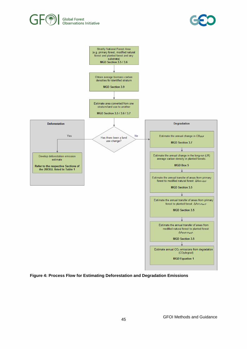
Figure 4: Process Flow for Estimating Deforestation and Degradation Emissions
GFOI Methods and Guidance
45

Box 4: Stratification
Stratification is the process of aggregating a population into sub-populations, or strata. It is commonly undertaken to improve sampling efficiency and may be required to allow reporting on separate and discrete sub-populations (e.g. primary forest versus modified natural forest). Stratification allocates individuals to relatively homogeneous groups so that individuals within one stratum are more likely to be similar to their neighbours than to individuals in another stratum. This grouping reduces the variance within each stratum, which will reduce the number of samples that are required to meet an overall precision target for sampling precision. Stratified sampling is one of the most commonly used design-based sampling approaches and allows unbiased inferences to be made of strata means, totals and variance.
To work properly, all members in the original population need to be assigned to one of the strata with no overlap or omission. There are many ways of stratifying a forest and some are more effective than others. The aim is to take advantage of available information about the population with the purpose of improving the precision of the estimate or usefulness of the inferences. A useful basis for stratification can be ecosystem type– e.g. some IPCC data divide tropical forest into wet, moist, dry and montanea. Remote sensing data in combination with supplementary ground-based data which maps the occurrence of forest ecosystems within an overall forest boundary using relief, climate and other relevant geographical factors is commonly used to identify forest strata.
Likelihood of human disturbance can also be the basis for further stratification. Identification of areas at high risk of deforestation can assist in designing early warning and targeted monitoring using high resolution images. This can be done using a statistical model that classifies the risk of disturbance in terms of the distance from already deforested areas, geographical determinants, and proximity to other factors such as transport infrastructure, agricultural or other relevant activities such as mining. Countries may wish to develop a statistical model from scratch, commission one, or take advantage of existing software to do this.
Suitable multiple spatial modelling programs exist including:
• Geomod/IDRISI (http://www.clarklabs.org/applications/Forest
• Land Change Modeler (http://www.clarklabs.org/products/Land-Change-Modeler-Overview.cfm)
• Dinamica (http://www.csr.ufmg.br/dinamica/)
GIS software combined with stratification can be an effective way of examining historic deforestation and determining factors that correlate with the historical location of deforestation. Such factors include:
Distance to existing deforestation Distance to roads or rail or navigable rivers
Distance to settlements Distance to mills / processing plants
Distance to markets Forest class
Elevation Aspect
Soil type Climate
For the purpose of deforestation/degradation estimation all such data must be spatial in format so that specific instances of deforestation may be linked with a location specific level of the given factor. Modelling potential deforestation/degradation location can be a cost effective way to target early warning monitoring and the strategic use of high resolution imagery.
Under stratified random sampling approaches, once the strata are established, each stratum is sampled at random and inferences about totals, means and variances are made. The estimates for all strata are combined to give a relatively precise population estimate. Sufficient sample density is needed within each stratum to ensure estimates are reliable, however the sample density does not have to be identical for each stratum and can vary depending on variance, cost of measurement and size of the carbon pool / change expected (Annex D).
Some spatially formatted data are continuous rather than discrete. Continuous data may be arbitrarily divided into discrete classes for the purpose of defining strata, provided the boundaries are clearly identifiable. Alternatively, design- and model-based sampling approaches exist which may use the continuous data without the need for grouping into classes. For example the continuous data as an auxiliary variable in ratio or regression sampling approaches.
Notes: a the full IPCC list is Wet, Moist with short dry season, Moist with long dry season, Dry, Montane moist, Montane dry (see e.g. GPG2003, Table 3A.1.2: Above ground biomass in naturally regenerated forest by broad category.
GFOI Methods and Guidance
46

2.2.2 Forest degradation
There is wide agreement that forest degradation represents long-term loss of forest values, and that temporary loss due to harvest or natural disturbance in sustainably managed forest is not degradation.
For reporting on REDD+, carbon stock is the value under consideration, so degradation is interpreted here as the processes leading to long-term loss of carbon without land-use change, otherwise there would be deforestation. Since sustainable management may take other forest values52 into account, degradation based on long term loss of carbon is not necessarily the same as unsustainable forest management, more broadly defined. In this case any decreases in carbon stocks would be estimated through sustainable management of forests, using the method described below in section 2.2.4. Degradation may occur in any of the forest types considered. In terms of the stratification suggested by the FRA it may start from primary forest but does not have to do so. Modified natural forests, and planted forests are not degrading if the long-run average carbon stock is maintained, or is increasing. Degradation, as interpreted here, occurs in areas where long-run53 average carbon stock is decreasing, even if temporary increases of carbon stock occur. Regional estimates of degradation have been made in the range 5% to 132% of deforestation emissions (Houghton, et al., 2009) and other estimates have been made at 25% and 47% of deforestation emissions (Asner et al. 2005, Asner at al 2010). Although regrowth will have a significant offsetting effect, forest degradation is likely to be a significant source of GHG emissions globally. Degradation is typified by a change in forest structure and species composition may result in:
• sustained loss of C from biomass and dead organic matter (DOM) pools;
• sustained loss of soil C, especially from peat forests following drainage, fire or exposure after a reduction of canopy density;
• sustained increase in emissions of non-CO2 GHGs, especially from fire.
Neither the GPG2003 nor the 2006GL identifies forest degradation by name, but since it occurs on Forest Land and does not entail deforestation, GHG emissions associated with it should be estimated using the methodologies described for Forest Land remaining Forest Land set out in section 3.2.1 of the GPG200354. Detecting forest degradation and then estimating the resulting GHG emissions, requires reliable forest observation techniques, data and resources. Countries should build upon existing systems and capacities where these are available, and integrate degradation measurement systems into their NFMS so that forest degradation is detected and measured in a manner consistent with detection and measurement of other REDD+ activities.
52 E.g. biodiversity, fire control, water management or productive capacity 53 See Box 6 of the main MGD text 54 Corresponding to Section 4.2 of volume 4 of the 2006 GL
GFOI Methods and Guidance
47
Multiple human-induced and natural processes can cause or contribute to forest degradation e.g. unsustainable biomass removal from selective logging or fuelwood gathering, over-frequent prescribed burning, or drainage of peat soils. Factors such as climatic stress, wildfire and pest infestation or diseases, though they also occur in forest areas that are not degrading, may also contribute. Degradation will have a more lasting effect where the capacity to regrow is impaired (e.g., following soil erosion, through loss of seed banks, or fragmentation caused by deforestation in adjacent areas).
Degradation may be localised (e.g. where it involves the loss of individual trees or groups of trees) or widespread (e.g., through wildfires covering many thousands of hectares). Patterns vary from selective removal of individual trees or groups of trees, with the latter often leading to the creation of fragments which are more susceptible to further degradation. Degradation can take place after a single disturbance event or through gradual processes. Use of remote sensing may significantly underestimate the extent of degradation (indicated by partial canopy cover reduction) for several reasons, depending on the pixel size of the imagery used and the time between image acquisitions over the area of interest. For example, in cases where there is canopy closure after disturbance there may only be a short time period in which degradation can be detected by remote sensing. In other cases, the nature of partial canopy reduction may be below the minimum extent detectable by the satellite. The extent of underestimation can be reduced by using high spatial and temporal resolution data (which is more likely to detect disturbances) and by constraining data analysis so that the transition from MNF to primary forest is not allowed – that is to say once forest has been disturbed, it is assumed to remain so.
In applying the IPCC methods countries are advised to follow the steps set out below. If both forest degradation and deforestation are considered, estimates need to be consistent. In particular, the stratification called for is the same as for deforestation, and steps 1) and 2) below are common with steps 1) and 2) identified above for estimating emissions from deforestation. Step 4) below is not exactly the same as step 3) under deforestation, because the former refers to a long-run average carbon density and the latter to a current value, but the calculation methods are similar and should be consistent. Degradation as estimated by the steps below takes account of long-term reductions of carbon densities due to transitions between forest strata and sub-strata, and within the strata and substrata affected by human activity (i.e. MNF and planted forests). For estimating degradation the steps are:
1) See step 1 under Deforestation (Section 2.2.1)
2) See Step 2 under Deforestation (Section 2.2.1)
3) Estimate the annual change in CBMNF. Call this quantity ΔCBMNF. It may be estimated from repeated NFIs if these exist, by sampling as set out below, by using the gain-loss method as set out in the GPG2003, section 3.2.1.1. It should take account of sub-stratification and factors including forest growth, logging, fuelwood harvest and fire. ΔCBMNF will be positive if CBMNF is increasing, and zero or negative otherwise. Set fMNF = 0 if ΔCBMNF is positive or zero and fMNF = +1 if ΔCBMNF is negative.
4) Estimate the annual change in the long-run (LR) average carbon density in planted forests. The long-run average carbon density is the carbon density averaged across the forest rotation taking account of both growth and harvesting events, and over successive forest rotations. This implies assessment of anticipated forest growth and removals due to harvest especially when there is a significant proportion of newly established planted forest in the planted forest estate. Call this quantity LRCBPlantF and the annual change ΔLRCBPlantF. First estimate LRCBPlantF for the
GFOI Methods and Guidance
48
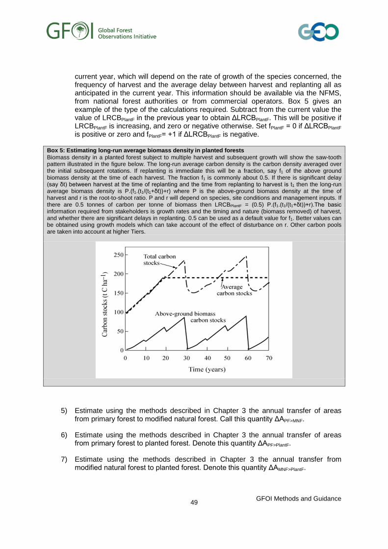
current year, which will depend on the rate of growth of the species concerned, the frequency of harvest and the average delay between harvest and replanting all as anticipated in the current year. This information should be available via the NFMS, from national forest authorities or from commercial operators. Box 5 gives an example of the type of the calculations required. Subtract from the current value the value of LRCBPlantF in the previous year to obtain ΔLRCBPlantF. This will be positive if LRCBPlantF is increasing, and zero or negative otherwise. Set fPlantF = 0 if ΔLRCBPlantF is positive or zero and fPlantF= +1 if ΔLRCBPlantF is negative.
Box 5: Estimating long-run average biomass density in planted forests Biomass density in a planted forest subject to multiple harvest and subsequent growth will show the saw-tooth pattern illustrated in the figure below. The long-run average carbon density is the carbon density averaged over the initial subsequent rotations. If replanting is immediate this will be a fraction, say f1 of the above ground biomass density at the time of each harvest. The fraction f1 is commonly about 0.5. If there is significant delay (say δt) between harvest at the time of replanting and the time from replanting to harvest is t1 then the long-run average biomass density is P.(f1.(t1/(t1+δt))+r) where P is the above-ground biomass density at the time of harvest and r is the root-to-shoot ratio. P and r will depend on species, site conditions and management inputs. If there are 0.5 tonnes of carbon per tonne of biomass then LRCBPlantF = (0.5) P.(f1.(t1/(t1+δt))+r).The basic information required from stakeholders is growth rates and the timing and nature (biomass removed) of harvest, and whether there are significant delays in replanting. 0.5 can be used as a default value for f1. Better values can be obtained using growth models which can take account of the effect of disturbance on r. Other carbon pools are taken into account at higher Tiers.
5) Estimate using the methods described in Chapter 3 the annual transfer of areas from primary forest to modified natural forest. Call this quantity ΔAPF>MNF.
6) Estimate using the methods described in Chapter 3 the annual transfer of areas from primary forest to planted forest. Denote this quantity ΔAPF>PlantF.
7) Estimate using the methods described in Chapter 3 the annual transfer from modified natural forest to planted forest. Denote this quantity ΔAMNF>PlantF.
GFOI Methods and Guidance
49

8) Estimate annual CO2 emissions from degradation (CO2degrad) using the following equation. The significance of the individual terms is described in the steps above and summarized in the Table 2:
CO2degrad = ΔAPF>MNF [CBPF − CBMNF] + ΔAMNF>PlantF [CBMNF − LRCBPlantF] +
ΔAPF>PlantF [CBPF − LRCBPlantF]
+(fMNF)(AMNF)|ΔCBMNF|+ (fPlantF )(APlantF)|ΔLRCBPlantF| ……(1)
Inclusion of a quantity in square brackets means that, if negative, the quantity should be treated as zero, so that the corresponding term will not then affect the total emissions from degradation. The fPlantF and fMNF multipliers perform a similar function so that only long-run decreases in carbon stock contribute to degradation. Vertical lines mean that the absolute value of the quantity which they enclose should be used. The table below shows the degradation processes to which the five terms on the right hand side of the equation respectively correspond. Since the terms are separately identified, degradation may be disaggregated by process or treated as a sum over processes. For example, if countries wish to distinguish between degradation which may occur in primary and modified natural forest (on the one hand) and that which may occur in planted forest (on the other) then the 5th term in equation (1) should be removed, and treated separately. The terms in the equation should be sub-divided to take account of sub-stratification.
Table 2: Terms used in Equation 1
Number of term on RHS of equ 1
Degradation process Term on the right hand side of equation 1
1 Conversion of primary forest to modified natural forest ΔAPF>MNF [CBPF – CBMNF]
2 Conversion of modified natural forest to planted forest ΔAMNF>PlantF [CBMNF − LRCBPlantF]
3 Conversion of primary forest to planted forest ΔAPF>PlantF [CBPF − LRCBPlantF]
4 Decrease in long-term carbon density of modified natural forest
(fMNF)(AMNF)|ΔCBMNF|
5 Decrease in long-term carbon density of planted forest (fPlantF)(APlantF)|ΔLRCBPlantF|
At Tier 1, GPG2003 assumes that for Forest Land remaining Forest Land, mineral soil, dead wood and litter pools are in equilibrium. If higher Tier methods are being used, national data should enable equation (1) to be expanded to include them. If organic soils are drained to establish planted forest, then emissions should be estimated for the corresponding planted forest areas as set out in Section 3.2.1.3 of GPG2003. Tier 1 CO2 emission factors reported in the IPCC guidance and guidelines for organic soils under different circumstances are summarised in Table 3.
GFOI Methods and Guidance
50
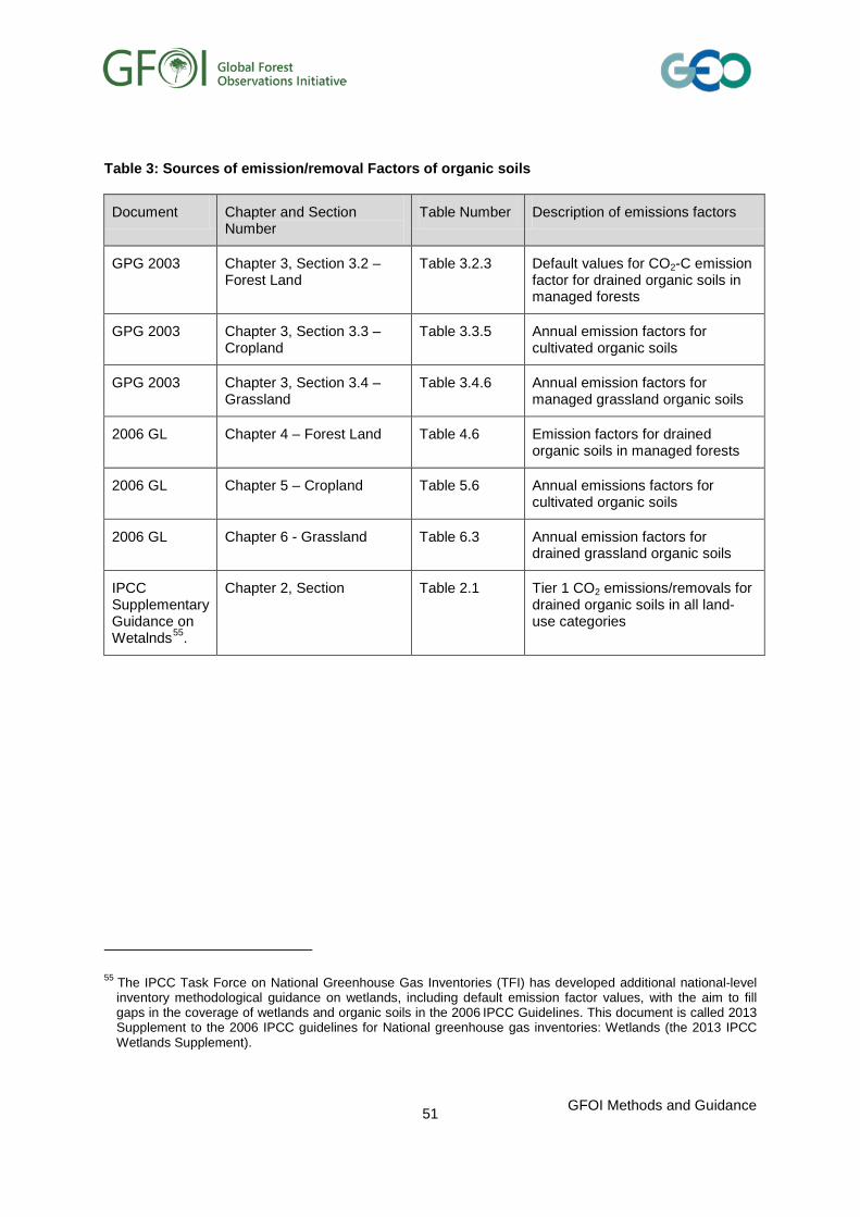
Table 3: Sources of emission/removal Factors of organic soils
Document Chapter and Section Number
Table Number Description of emissions factors
GPG 2003 Chapter 3, Section 3.2 – Forest Land
Table 3.2.3 Default values for CO2-C emission factor for drained organic soils in managed forests
GPG 2003 Chapter 3, Section 3.3 – Cropland
Table 3.3.5 Annual emission factors for cultivated organic soils
GPG 2003 Chapter 3, Section 3.4 – Grassland
Table 3.4.6 Annual emission factors for managed grassland organic soils
2006 GL Chapter 4 – Forest Land Table 4.6 Emission factors for drained organic soils in managed forests
2006 GL Chapter 5 – Cropland Table 5.6 Annual emissions factors for cultivated organic soils
2006 GL Chapter 6 - Grassland Table 6.3 Annual emission factors for drained grassland organic soils
IPCC Supplementary Guidance on Wetalnds55.
Chapter 2, Section Table 2.1 Tier 1 CO2 emissions/removals for drained organic soils in all land-use categories
55 The IPCC Task Force on National Greenhouse Gas Inventories (TFI) has developed additional national-level inventory methodological guidance on wetlands, including default emission factor values, with the aim to fill gaps in the coverage of wetlands and organic soils in the 2006 IPCC Guidelines. This document is called 2013 Supplement to the 2006 IPCC guidelines for National greenhouse gas inventories: Wetlands (the 2013 IPCC Wetlands Supplement).
GFOI Methods and Guidance
51

2.2.3 Sustainable management of forests, enhancement of C stocks (within an existing forest), and conservation of C stocks
These activities are likely to be associated with specific national and regional policies, which may be linked to particular geographical areas, consistent with national strategies for sustainable management, implying need for appropriate sub-stratifications.
Recognising that countries will have national forest definitions, there seems wide agreement that sustainable management of forests aims to maintain and enhance forest values56. This does not necessarily mean maintaining the carbon stocks initially present in primary or modified natural forests. For example, average biomass carbon stocks are always less in harvested forests than in equivalent forests that are not subject to harvest, but in a sustainably managed production forest carbon stocks would not decline (thus reflecting sustained productive capacity) over time when averaged over harvesting cycles. Conservation of carbon stocks aims to maintain carbon stocks. Enhancement of carbon stocks aims to increase carbon stocks, which could be within an existing forest area, or by converting another land use to forest. This second possibility is methodologically distinct because it entails land-use change, and is dealt with separately below. Enhancement of carbon stocks (within an existing forest), conservation of carbon stocks, and sustainable management of forests would all occur within existing forest areas that remain forest areas. Therefore, as with degradation, GHG emissions and removals associated with them should be estimated using the methodologies described for Forest Land remaining Forest Land set out in section 3.2.1 of the GPG200357. These methods address above- and below-ground biomass, litter, dead wood and soil organic matter and associated emissions of non-CO2 GHGs.
2.2.4 Estimation of emissions and removals for sustainable management of forests, enhancement of carbon stocks (within an existing forest), and conservation of carbon stocks
Since these activities are generally intended to maintain or increase forest carbon stocks, they are the reverse of degradation, and sometimes the same activity can lead to degradation or the reverse, depending on the intensity, an example being harvesting. Estimation of carbon change for the above activities should therefore be consistent with estimation for degradation. Therefore to estimate emissions and removals from sustainable management of forests, enhancement of carbon stocks (within an existing forest), and conservation of carbon stocks, countries are advised to follow steps 1 to 9 set out above for degradation, in the following way:
• Within the stratified areas, for example primary forest, modified natural forest and planted forest, if there are particular areas subject to sustainable management activities, use remote sensing data in combination with information from national
56 Although the language refers to sustainable forest management rather than sustainable management of forests, the UN has recognised that sustainable forest management, as a dynamic and evolving concept, aims to maintain and enhance the economic, social and environmental values of all types of forests, for the benefit of present and future generations (Non-legally binding instrument on all types of forests, adopted by the UN General Assembly 22 Oct 2007)
57 Corresponding to Section 4.2 of volume 4 of the 2006 GL
GFOI Methods and Guidance
52

forestry authorities to identify these as sub-strata. This step will be unnecessary if all the strata are subject to sustainable management.
• The equation for estimating emissions and removals from these activities becomes:
CO2sust = ΔAPF>MNF(CBPF − CBMNF)+ΔAMNF>PlantF(CBMNF− LRCBPlantF)+
ΔAPF>PlantF(CBPF − LRCBPlantF) − AMNF(ΔCBMNF) − APlantF (ΔLRCBPlantF ) ……(2)
This version of the equation assumes that all the forest remaining forest is subject to the activities sustainable management of forests, enhancement of carbon stocks (within an existing forest), and conservation of carbon stocks; and all terms contribute to the total irrespective of sign. The equation is arranged so that CO2sust will be negative (corresponding to a removal) if carbon stocks are increasing. The equation assumes that primary forest can become modified natural forest or plantation forest, and that modified natural forest can become planted forest, but that the reverse transitions do not occur. The table below shows the processes to which the five terms on the right hand side of the equation respectively correspond. Since the terms are separately identified, emissions and removals from these activities may be disaggregated by process or treated as a sum over the processes involved.
Table 4: Terms used in Equation 2
Number of term on RHS of equ 2
Process Term on the right hand side of equation 2
1 Conversion of primary forest to modified natural ΔAPF>MNF(CBPF − CBMNF)
2 Conversion of modified natural forest to planted forest ΔAMNF>PlantF(CBMNF − LRCBPlantF)
3 Conversion of primary forest to planted forest ΔAPF>PlantF(CBPF − LRCBPlantF)
4 Change in long term carbon density of modified natural forest
AMNF(ΔCBMNF)
5 Change in long term carbon density of planted forest APlantF (ΔLRCBPlantF )
If a transition occurs in a partitioned forest type, the carbon densities to use are those which correspond to the transition being made. If primary forest is successfully conserved then ΔAPF>MNF and ΔAPF>PlantF will both be zero.
If forest degradation and the sustainable activities are both present, then to avoid double-counting:
GFOI Methods and Guidance
53

• if emissions from degradation and the sustainable activities are to be separately identified, degradation should be estimated using equation (1) and the sustainable activities then estimated as the difference between equation (1) and (2). If equation (1) has been disaggregated in some way, e.g. by treating planted forests separately, then equation (2) should be disaggregated in the same way.
• if all degradation and the sustainable activities are to be estimated together only equation (2) should be applied. Since there are no sign restrictions in equation (2) any degradation which occurs within activities defined as sustainable management of forests, enhancement of carbon stocks (within an existing forest), and conservation of carbon stocks will be included in the emissions estimate.
2.2.5 Enhancement of forest carbon stocks (afforestation of land not previously forest, reforestation of land previously converted from forest to another land use)
In addition to enhancement within existing forests, forest carbon stocks can be enhanced by establishing forests on land which was not previously forest, or which had earlier been converted from forest to another land use. Forest establishment on such land will result in carbon accumulation in biomass, though initially the loss of soil carbon due to disturbance of carbon stocks in mineral soils may exceed the biomass accumulation; and if organic soil has been drained, this loss will continue as long as the drainage continues. Accumulation of biomass will follow a sigmoid curve, with rates varying with species, site growing conditions and age. Harvest will interrupt the sigmoid accumulation of biomass (with disturbance emissions) with growth resuming again after replanting. This produces the characteristic saw-tooth curve illustrated in Box 5. Harvesting with replanting is part of a forest management cycle and does not constitute deforestation, or degradation provided the average carbon stock is maintained in the long run. Planted forests established for environmental values will not necessarily be harvested, and if they are not, the initial sigmoid will proceed to saturation at the carbon carrying capacity of forest on the land concerned, and there will be no saw-tooth pattern. Consistent with the 2003GL, emissions and removals on unmanaged58 land are not included in GHG inventories so it is assumed that forest expansion on unmanaged land will not count towards this activity. Consistent with the agreed safeguards59, REDD+ actions should not be used for conversion of natural forest.
2.2.6 Estimation of emissions from enhancement of forest carbon stocks (afforestation of land not previously forest, reforestation of land previously converted from forest to another land use)
Since this entails a conversion of another land use to forest it corresponds directly to section 23.2.2 of GPG2003, Land Converted to Forest Land, corresponding to section 4.3 in volume 4 of the 2006GL. In applying the IPCC methodology countries should:
1) Via the NFMS, collect information on forest establishment on lands not previously forested, or on lands which were once forested but have been converted to another land use. Information may be available from stakeholders, government departments or forestry authorities (all of whom should be represented on the NFMS) on tracking
58 See Chapter 1 for a discussion of forest definitions including managed and unmanaged forest. 59 See paragraph 2(e) of Appendix 1 to the Cancun Agreements contained in decision 1/CP.16.
GFOI Methods and Guidance
54

concessions and planting permits. Remote sensing may not always be a useful data source for this step, because forests in the early stage of growth are not easily distinguished by remote sensing. It may be possible to detect signs of preparation and planting work and this can be used as supporting information. The information sought should include type of forest established, planting date, and if possible a management plan.
2) As the planted forest grows following establishment, use remotely sensed data to confirm the forest areas and timing of harvest activities and resolve any differences with the information obtained under 1). This will improve the accuracy of results.
3) In making national estimates, emissions and removals associated with this activity should be included with those from sustainable management of forests, enhancement of C stocks (within an existing forest), and conservation of C stocks
2.2.7 Conversion of natural forest
The Cancun Agreements list conversion of natural forest under safeguards provisions, not as a REDD+ activity. The Agreements specify60 the need to promote and support safeguards … consistent with the conservation of natural forests and biological diversity, ensuring that [REDD+ activities] are not used for the conversion of natural forests, but are instead used to incentivize the protection and conservation of natural forests and their ecosystem services, and to enhance other social and environmental benefits. The annual area converted can be
calculated as the sum Ʃi=1,5 A(1,i) where j=1 is taken to be the index for primary forest at step 5 above under deforestation emissions estimation, plus the transfer rates from modified natural forest to planted forest and from primary to planted forest, ΔAMNF>PlantF and ΔAPF>PlantF estimated respectively at steps 5 and 6 under degradation emissions estimation. This covers conversion of natural forest to non-forest land uses, and to other forest types. The emissions associated with these transfers can be estimated from the application of the IPCC methods identified above to these transferred areas.
60 See paragraph 2(e) of Appendix 1 to the Cancun Agreements contained in decision 1/CP.16.
GFOI Methods and Guidance
55
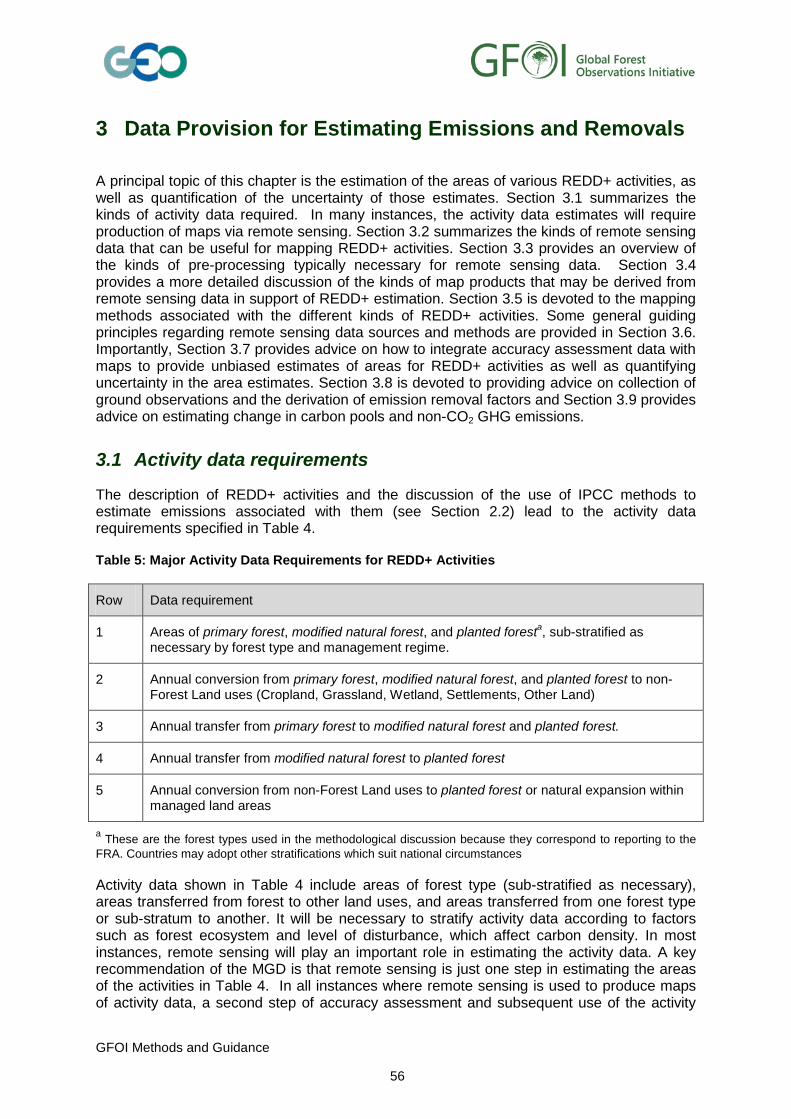
3 Data Provision for Estimating Emissions and Removals
A principal topic of this chapter is the estimation of the areas of various REDD+ activities, as well as quantification of the uncertainty of those estimates. Section 3.1 summarizes the kinds of activity data required. In many instances, the activity data estimates will require production of maps via remote sensing. Section 3.2 summarizes the kinds of remote sensing data that can be useful for mapping REDD+ activities. Section 3.3 provides an overview of the kinds of pre-processing typically necessary for remote sensing data. Section 3.4 provides a more detailed discussion of the kinds of map products that may be derived from remote sensing data in support of REDD+ estimation. Section 3.5 is devoted to the mapping methods associated with the different kinds of REDD+ activities. Some general guiding principles regarding remote sensing data sources and methods are provided in Section 3.6. Importantly, Section 3.7 provides advice on how to integrate accuracy assessment data with maps to provide unbiased estimates of areas for REDD+ activities as well as quantifying uncertainty in the area estimates. Section 3.8 is devoted to providing advice on collection of ground observations and the derivation of emission removal factors and Section 3.9 provides advice on estimating change in carbon pools and non-CO2 GHG emissions.
3.1 Activity data requirements
The description of REDD+ activities and the discussion of the use of IPCC methods to estimate emissions associated with them (see Section 2.2) lead to the activity data requirements specified in Table 4.
Table 5: Major Activity Data Requirements for REDD+ Activities
Row Data requirement
1 Areas of primary forest, modified natural forest, and planted foresta, sub-stratified as necessary by forest type and management regime.
2 Annual conversion from primary forest, modified natural forest, and planted forest to non-Forest Land uses (Cropland, Grassland, Wetland, Settlements, Other Land)
3 Annual transfer from primary forest to modified natural forest and planted forest.
4 Annual transfer from modified natural forest to planted forest
5 Annual conversion from non-Forest Land uses to planted forest or natural expansion within managed land areas
a These are the forest types used in the methodological discussion because they correspond to reporting to the
FRA. Countries may adopt other stratifications which suit national circumstances
Activity data shown in Table 4 include areas of forest type (sub-stratified as necessary), areas transferred from forest to other land uses, and areas transferred from one forest type or sub-stratum to another. It will be necessary to stratify activity data according to factors such as forest ecosystem and level of disturbance, which affect carbon density. In most instances, remote sensing will play an important role in estimating the activity data. A key recommendation of the MGD is that remote sensing is just one step in estimating the areas of the activities in Table 4. In all instances where remote sensing is used to produce maps of activity data, a second step of accuracy assessment and subsequent use of the activity
GFOI Methods and Guidance
56

data to correct for biases that may exist in the maps is essential. One added benefit of this approach is that it allows for quantification of the uncertainties (in the form of confidence intervals) for the activity data.
3.2 Remote sensing data sources
The MGD anticipates that medium- and high-resolution optical and radar data are the main types of remotely sensed data that will be used to apply the estimation methods for the REDD+ activities it describes. Currently there is most experience with using medium resolution optical data. This is because:
• there is experience in the use of data of this type by countries in making national emissions estimates from deforestation and from LULUCF activities;
• Landsat provides an historical archive of data of this type back to the early1970s and, given the successful operations of the most recent Landsat 8, there is the prospect of continuing availability of data for the foreseeable future;
• Landsat data are acquired globally and are freely available in pre-processed form, and new techniques in data mining or compositing can do much to mitigate problems of interference by cloud cover. Visual interpretation can also help increase accuracy where there is poor temporal coverage due to cloud.
The near-future availability of longer wavelength (L-band) SAR data is likely to result in its increasing inclusion in national forest monitoring systems. There is currently no satellite providing L-band SAR data in operation, but two missions are anticipated in 2014 and 2015 (ALOS-2 and SAOCOM-1). L-band SAR has potential for mapping forest and land cover and change, in particular in areas of persistent cloud cover. There are many pre-operational demonstrations of the utility of L-band SAR for REDD-related activities. Historic global L-band SAR coverages are available from the mid-1990s and for the period 2007-2011 for establishing a forest baseline and decadal forest change monitoring. There is ongoing research in the use of L-band SAR for detecting degradation and estimation of above-ground biomass. Likewise as methods development progresses in the use of dense time series C-band SAR for monitoring activity data, countries may consider to make use of future Sentinel-1 acquisitions. Joint use of C and L band data is likely to increase the accuracy of forest: non-forest classification. Tropical countries have indicated a desire to use SAR together with optical data to fill data gaps and provide additional information on forest stratification and biomass.
Experience is increasing with the application of high resolution optical data61, which is likely to increase accuracy in identifying land subject to degradation, and may be needed for complete detection of forest where a small minimum area is used in the national forest
61 For example Guyana and Mexico are using high resolution data, in the former case to monitor degradation and in the latter because of small minimum area in the national forest definition.
GFOI Methods and Guidance
57

definition. Box 6 summarises Guyana’s experience with using high resolution data in an operational MRV system that can map degradation.
The main data types are described below. Annex B summarises optical and radar data availability at the time of writing, with information on spatial and temporal resolution and availability and also provides links to the CEOS website where more detail can be obtained.
3.2.1 Coarse resolution optical data
Coarse resolution refers to a pixel size of greater than about 250m which is generally regarded as too large to be used for generating REDD+ activity data. Changes in spectral indices derived from coarse resolution data e.g. MODIS62 and CBERS-2 may be useful in detecting areas where changes are occurring in forests, and this can be used for stratification or to guide sampling. High temporal resolution available from MODIS can help compensate for the coarse spatial resolution by smoothing the time series63. High frequency, coarse resolution data can be used to derive a near-real time forest change indicators map, useful for early warning and detection of forest clearing and degradation.
3.2.2 Medium resolution optical data
Medium resolution lies in the range 10 to 80 metres. The most common imagery which may be used for monitoring REDD+ activities is 30 metre resolution, from the Landsat series of satellites (GOFC-GOLD Sourcebook, 2012). Advantages associated with Landsat data include (a) a long history of use, (b) global acquisition, pre-processing and archiving of data, (c) free access to data in the US archive. Landsat will often be the only dataset available for estimating historical activity data. The data series goes back to the 1970s and the successful launch of the Landsat 8 in February 2013 continues the time series for the foreseeable future. The use of optical sensors is a limitation in areas with persistent cloud cover. Nevertheless the accessibility and global coverage associated with Landsat generally make it the first data source to consider for a NFMS. For many purposes Landsat will serve to fulfil national remote sensing data requirements associated with REDD+ activity data collection. The CBERS-4 and Sentinel 2 satellites will increase availability of medium resolution data, including by making 10 m resolution data freely available and facilitating applications which have hitherto been regarded as only possible at high resolution. Spectral indices derived from optical data can in some cases be linked to biomass, but there are issues with saturation above a certain biomass density and this is not currently used in GHG inventory estimation (Powell, et.al., 2010).
Countries having national operational programs for forest cover monitoring using Landsat or Landsat-like data include Australia (Furby et al 2008), Brazil (DMC and CBERS; Souza, 2006), India (IRS; Pandy, 2008) and the United States (Fry et al 200964).
The remote sensing data must be pre-processed as described in Section 3.3 to provide a common basis for comparison with other data.
62 Available free from NASA on http://reverb.echo.nasa.gov/reverb/ 63 http://ivfl-info.boku.ac.at/index.php/eo-data-processing 64 Available at http://pubs.usgs.gov/of/2008/1379/pdf/ofr2008-1379.pdf
GFOI Methods and Guidance
58

Box 6: Development of an operational MRV system incorporating High Resolution Data – Case Study Guyana
In 2008, Guyana launched its Low Carbon Development Strategy (LCDS) which provides the framework for REDD+ activities. Guyana has an MRV system which provides the basis for performance measurement. The development of the MRV system stems from a capacity building Roadmapa spanning the period 2010 to 2013, and includes the forest carbon monitoring system and forest cover assessment. The work has been supported under the terms of the Joint Concept Note which Guyana and Norway signed in 2009b.
Like many countries Guyana began developing its historical (1990) land cover change baselines from freely-available 30 m Landsat imagery. After the first year of operation (2011), the Guyana Forestry Commission (GFC)c reviewed the MRVS progress and opted for high resolution RapidEye imagery to cover the most active change areas. Today the MRV system conforms to IPCC approach 3. All post 1990 land cover changes (including non-anthropogenic ones) greater than 1 ha are detected, mapped and stored as a GIS. From 2011 onwards the MRV system included the mapping and monitoring of forest degradation (or canopy disturbance) surrounding deforestation events at a national-scale. An independent accuracy assessment conducted in 2013 quantified the accuracy of the deforestation and forest degradation mapping at 99% and 80%d respectively.
The process designed and adopted by GFCe has developed over time, and integrates GPG linked to operational research focused on developing methods appropriate for the drivers responsible for forest degradation in Guyana. The MRV system design recognises the problem of persistent cloud cover, the spatial scale and the intensity of the land cover change. To address these, frequent coverage of high resolution imagery is used. As with many countries, considerable expertise in Guyana resides in the use of GIS rather than in remote sensing technologies. Given these challenges, a GIS-based MRV system has the advantage of being adaptable, user friendly and flexible enough to incorporate a range of different data types required to meet IPCC requirements.
The change detection processing chain is semi-automated with each satellite image assimilated and batch processed. The processing includes conversion of images to reflectance, atmospheric normalisation, detection and delineation of land cover change using vegetation indices, and conversion of these changes to a GIS format. The quality of the change delineation is systematically assessed and edited by trained analysts who also attribute a change driver to each polygon. The attribution options are illustrated in mapping guidance documentation with the attribution process controlled by the use of a customised GIS toolbar. The toolbar stores all relevant attributes and assists the operator to ensure appropriate land cover change and driver combinations are selected. Figure 1.1 provides an overview of the mapping flow, from satellite images (A) to creation of a pre-processed change layer (B) to the generation of a multi-temporal forest change products (C).
Figure 1.1 Mapping Process
Forest degradation mapping is undertaken in conjunction with deforestation mapping. The scale (<1 ha) and intensity of degradation is known to vary by driver (i.e. mining prospecting, timber extraction, or shifting cultivation). Degraded forest is identified from temporal persistence of canopy disturbance. Further monitoring is used to determine if the changes in the canopy can be considered forest degradation, linked to a significant percentage reduction in carbon stocks in the areas affected, or just temporary disturbances that recover in a short time period. To detect forest degradation on satellite imagery the disturbance must occur at a scale that causes a visible change in the canopy. Using the method adopted, the pixel resolution and temporal frequency of sensors such as Landsat and DMC are insufficient to detect forest degradation related to canopy disturbance. Notes: a. http://www.forestry.gov.gy/publications.html, b. The JCN sets out a series of interim measures that are intended to be used whilst the full MRV System is being developed. c. The implementing Agency with technical assistance provided by Indufor Asia Pacific d. Results of the independent accuracy assessment are presented in Guyana’s Year 3 MRVS e. http://www.forestry.gov.gy
Normalised Imagery (A) Change Detection (B) Attributed Change (C)
GFOI Methods and Guidance
59

3.2.3 High resolution optical data
High resolution data (resolution better than 10 metres) can improve detection of changes associated with degradation, and allow REDD+ activity data generally to be monitored more accurately and with greater differentiation than medium resolution data. Acquisition and processing costs are higher, and high resolution data may not be available for entire countries for a sufficient number of time periods to allow direct estimation of REDD+ activity data from complete (wall-to-wall) coverage. For these reasons high resolution optical data have hitherto been used mainly in sample-based verification or accuracy assessment, for sampling transects or local areas or regions of interest, and for assessment of hot spots where changes are occurring or are more likely to occur. Some countries are now using high resolution data for wall to wall mapping65 (see Box 6 for case study on Guyana’s Mapping approach). High resolution data may also be valuable for providing training data for change detection algorithms and can be used to produce emission and removal factors – e.g. the application of LiDAR (see below) to estimating depth of peat combusted by fire in Indonesia, and hence emissions of CO2 and non-CO2 greenhouse gases (Ballhorn, et al., 2009). The use of high resolution data continues to be the subject of research.
3.2.4 Synthetic aperture radar
The potential ability of imaging radar (also referred to as Synthetic Aperture Radar or SAR) to provide activity data has been demonstrated at the sub-national (Mitchell et al, 2012) and regional (project) level and could be useful particularly in areas of persistent cloud cover, also in combination with optical data. Radar sensors operating at different wavelengths are sensitive to different features on the ground and as a generality, radar can be said to be sensitive to objects that are of similar size or larger, than the radar wavelength. Current and near-future SAR systems furthermore have multi-polarisation capacities which, like the different spectral bands of optical data, provide additional information. Radar systems can provide information that is not visible in optical data (and vice versa) and the two data sources are therefore to be regarded as complementary, not competing.
An additional advantage of radar’s independence of cloud cover is that large regions can be acquired within relatively short time windows (few weeks – few months) so reducing the need to fill in data gaps with data from different years or different seasons. Consistent archives of global or regional wall-to-wall data exist for some historical SAR missions for certain time periods (JERS-1 SAR, ALOS PALSAR), and through the CEOS Data Strategy for GFOI, such systematic acquisition strategies are becoming standard for several of the near-future core and non-core SAR missions (Sentinel-1, SAOCOM-1, ALOS-2, RCM).
In heavily cloud-affected areas, L-band SAR provides a useful alternative data source for stratifying by forest and non-forest. Although not currently used operationally, there are several sub-national demonstrations of wall-to-wall forest area (Mitchell, 2012; GEO, 2011; Walker et al 2010) and change mapping (Kellndorfer, et al., 2008) using time series of ALOS PALSAR fine beam dual (FBD) polarisation data. L-band SAR-based forest mapping methods are advanced, and currently mainly limited by data supply (hence referred to as pre-operational). With the upcoming launch of new L-band SAR satellites (SAOCOM-1A and -1B, ALOS-2), followed by systematic wall-to-wall acquisition at regional/global scale, pre-operational SAR-based methods may be adopted into more operational processing streams. Dense time series of C-band SAR data can also be used to detect forest area changes
54 Countries include Guyana and Mexico
GFOI Methods and Guidance
60
relative to a pre-determined forest area. Where available, the integration of optical and L-band SAR data is likely to be advantageous, and is the subject of ongoing research.
3.2.4.1 L-band SAR With a wavelength of about 23.5 cm, L-band SAR penetrates through the forest canopy and generally provides clear distinction between vegetated and non-vegetated areas. It is commonly used for mapping of forest/non-forest, and with time series of data, for detection of forest cover changes. At least two polarisations are preferred, because the cross-polarisation channel is found to be particularly sensitive to forest structural parameters, such as twigs, branches and stems, and thus indirectly to forest types and age classes. L-band SAR is also linked to above-ground biomass up to a level of about 100 tonnes per hectare, although this is an area of research (Lucas, et al., 2010; GEO, 2011) and accuracy levels are currently insufficient for use for greenhouse gas inventory estimates.
Semi-annual wall-to-wall observations over the global forest cover were undertaken by ALOS L-band SAR (PALSAR) between 2007 and 2011. Both ALOS-2 (launch 2014) and SAOCOM-1A and -1B (launch 2015 and 2016) have similar systematic global acquisition strategies that will continue to provide cloud-free coverage of the global (ALOS-2) or pan-tropical (SAOCOM) regions several times per year.
High temporal frequency, coarse (100 m) resolution L-band SAR data acquired in so-called ScanSAR mode have demonstrated potential for early warning of forest clearings (e.g., INDICAR system of IBAMA, Brazil (de Mesquita, 2011).
L-band SAR is considered to have operational capacity to map forest cover and changes (GEO, 2011; Walker et al, 2010), and to have pre-operational capacity to derive land cover (GEO, 2011), activity data (Mitchell et al, 2012; Lucas, et al., 2010), forest sub-stratification (GEO,2012; Hoekman, 2012) products as input to emissions estimation. Combined use of different sensor types (e.g. L-band SAR and optical, L- and C-band SAR) can improve discrimination of forest and land cover types (Holecz et al, 2010).
3.2.4.2 C-band and X-band SAR SAR systems operating at shorter wavelengths (C-band: 5.6 cm; X-band: 3.1 cm) typically reflect from the surface and top layer of the forest (leaves and twigs) and thus provide information about canopy structure. While the contrast between forest and low vegetation generally is less distinct compared with longer wavelength SAR, the use of two polarisations improves discrimination. X-band SAR data can be acquired at a spatial resolution better than 5 metres, which allows more detailed characterisation of forest canopy structure and although still regarded as research, has potential to provide information about forest degradation (e.g., selective logging (Baldauf, 2013)).
Frequent time series of C-band SAR data has demonstrated capacity for detection of changes in forest cover, and has potential for use for early warning of forest clearing. To avoid confusion with changes occurring in other land cover classes, change detection can be applied relative to a pre-determined forest area derived e.g. from optical or L-band SAR data.
GFOI Methods and Guidance
61

Once in full-scale operation, C-band core missions Sentinel-1A and -1B (launch 2013 and 2014) are scheduled to provide intra-annual observations of all global land areas, with potential higher frequency observations over selected countries or regions. Amongst non-core missions, a full global coverage of X-band SAR data have been collected by the TanDEM-X satellite constellation.
3.2.5 LiDAR
LiDAR sensors emit pulses in near-infrared wavelengths that interact with different strata and from which quantitative information on forest structure (e.g., tree height, canopy volume) and biomass can be estimated. LiDAR-assisted biomass estimation using wall-to-wall coverage of satellite data is a research topic of interest for future forest monitoring systems and this use of LiDAR is discussed in Annex F. Although an historic archive of satellite LiDAR is available 66, there are currently no operational LiDAR satellites. The ICESAT-2 mission for a space-borne LiDAR is planned to be launched in early 2016. Subject to the demonstration of suitable techniques, space-borne LiDAR could be used for estimation and cross-checking with other methods. Airborne LiDAR can be used for verification of biomass estimates and to reduce the need for ground sampling for biomass estimation, particularly in areas where ground access is difficult and hence expensive.
3.3 Pre-processing of satellite data
Satellite observations from one time period need to be aligned so that they can be compared and used to identify areas and changes. The steps required to do this are called pre-processing.
Pre-processing involves geometric and radiometric calibration, and in the case of SAR data, speckle filtering. Geometric calibration, also called orthorectification, corrects for the angle of view of the satellite sensor, the relief of the terrain and lens distortions so that images from different sensors at different times can be compared in the same way as maps made using the same projection and scale can be compared. Radiometric calibration is needed because the appearance of the same image varies with angle of view and illumination conditions.
Orthorectification and radiometric calibration are often performed together because both require a digital elevation model (DEM). A common standard DEM is available from the Shuttle Radar Topography Mission (SRTM) at 3 arc second resolution (about 90 meters) or 1 arc sec, if available, via a data access agreement. Other suitable globally available DEMs include the 1 arc second ASTER DEM available for download from the Global Data Explorer 67 of the United States Geological Survey (USGS). Countries possessing higher accuracy DEMs (e.g., derived from stereogrammetry or LiDAR) may wish to use these in the orthorectification of data if the result would be increased accuracy and demonstrated benefit for the added cost.
If orthorectification is improperly done, areas of land use change may be overestimated and land use incorrectly assigned. Poorly co-registered data typically result in over-estimates of change, because any apparent changes due to misalignment of pixels (termed false change) will be reported in addition to real land cover changes. Minimising false change due to geometric errors in mapping forest and land cover should be the main objective in the
66 Refer to the ICESAT-GLAS data archive. Accessed at: http://icesat.gsfc.nasa.gov/ 67 http://gdex.cr.usgs.gov/gdex/
GFOI Methods and Guidance
62

selection and application of the pre-processing methodology for geometric calibration. As a result, co-registration of the time series of all remotely sensed data should be achieved at accuracy better than 1 pixel maximum error. Common controls, e.g. by matching of easily identifiable features, should be adopted when co-registering images. As the time series will progressively evolve, it will be necessary to establish a topographic reference to which all other images are co-registered. When combining sensors having oblique viewing geometries, co-registration may be improved by using a DEM with greater accuracy than the reference DEM, and this should be done if it improves the co-registration accuracy against the reference.
3.3.1 Pre-processing of optical satellite images
Consistent spatial and temporal calibration allows trends in land-cover to be quantified, enables automation of forest cover characterizations, and leads to reduced ground data requirements because areas with similar characteristics are easier to identify.
Radiometric calibration can be absolute where radiometric values are converted to a geophysical standard quantity such as surface reflectance, or relative where radiometric values are adjusted to a reference standard by comparing the reference ground reflector signatures to see if there are significant differences between sensors. Images need to be calibrated to the reference so that pixels in different images can be compared directly, no matter on which day or season the image was collected or under what sun-sensor-target geometry. The viewing geometry varies significantly across the path of the satellite resulting in very different reflectance values for the same land cover feature.
When comparing trends in reflectance across different optical sensors, it may be necessary to adjust for differing band pass68 characteristics, should they be significantly different. The need for correction can be established by comparing reference ground reflectance signatures to see whether there are differences between sensors. If there are, the difference can be removed by multiplying by the ratio of the standard reflectance signatures.
Where terrain has significant relief, it will also be necessary to normalise for the differential terrain illumination, using the same DEM that is used for other pre-processing steps.
Many data providers include some or all of the key pre-processing steps discussed in this section. Users should consider the advantages of using pre-processed data sets in facilitating monitoring objectives. For example, imagery from the Landsat series of satellites is provided free of charge through the Earth Resources Observation and Science Center (EROS) of the USGS69 (Woodcock et al. 2008). The imagery is delivered pre-processed. Imagery processed to level 1G (in the case of Landsat known as L1G) is radiometrically calibrated and geometrically corrected for distortions such as sensor jitter, view angle effects
68 Band pass refers to the frequency or wavelength range admitted by a filter.
69 http://earthexplorer.usgs.gov/ or http://glovis.usgs.gov/
GFOI Methods and Guidance
63

and Earth curvature (Landsat Science Data Users Handbook70). The Landsat L1T format provides globally available data, orthorectified to a consistent geometric standard using ground control points and the SRTM-derived DEM. This forms a de facto standard for optical image pre-processing, and is effectively a global default.
The Landsat Ecosystem Disturbance Adaptive Processing System (LEDAPS) allows for automatic estimation of surface reflectance from L1T imagery without any ancillary information required. The USGS currently delivers LEDAPS-processed Landsat TM and ETM imagery in the units of surface reflectance through Earth Explorer (see footnote 67 above), and atmospherically corrected Landsat-8/OLI imagery will be available in the near future. Atmospherically corrected Landsat L1T data provide geometrically and radiometrically consistent imagery highly suitable for mapping of REDD+ activities.
Other satellite imagery used for activity data mapping need processing to a level equivalent to L1T. This is often provided by the supplier but if not, the user has to complete these processing steps after data delivery. This can be accomplished with most standard image processing software such as ENVI and ERDAS. Hands-on advice is provided by image processing textbooks such as Jensen (2005) and software manuals.
3.3.2 Pre-processing of SAR satellite images
Like all radar, SAR relies on the relationship between an emitted and a reflected radio signal to detect interesting properties of the region of interest.
Radar signals need pre-processing to account for geometric distortions (e.g., layover71 and foreshortening), and for differences in illumination conditions due to topography and the surface being illuminated to one side of the satellite or aircraft. An additional step is needed to remove noise caused by reflections from features that are not of interest – e.g. minor irregularities. This is called speckle noise and is removed by a process called speckle filtering. Further details about pre-processing radar signals can be found in Mitchell et al, 2012 and free pre-processing software is available72.
There is a common misconception that the pre-processing and interpretation of radar data is overly complicated. GFOI will provide pre-processed radar data to interested countries, suitable for generation of forest map products. Visualisation and interpretation of radar data becomes easier once the principles of radar formation and interaction are known and understood. For those countries aiming to develop in-house capacity in the use of radar, GFOI will facilitate capacity building and training in software and processing workflows for use of radar data and implementation in existing forest monitoring systems.
A typical processing sequence applied to SAR data entails multi-looking, speckle filtering, orthorectification and radiometric calibration, terrain illumination correction and mosaicking73. The highest resolution Single Look Complex (SLC) product is quite noisy. Multi-looking averages over range and azimuth cells to improve radiometric resolution and produce near-
70 http://landsathandbook.gsfc.nasa.gov/
71 A distortion due to the radar beam reaching the top of an object before it reaches the base. Foreshortening occurs when the beam reaches the base before it reaches the top.
72 For example at http://nest.array.ca/web/nest 73 Mosaicking is producing a larger image by combining individual images.
GFOI Methods and Guidance
64

square pixels. Adaptive filters use local statistics to filter the data and so reduce image speckle and in some cases, preserve or enhance edges and other features.
As with optical data, SAR data are orthorectified and radiometrically calibrated to produce suitable images for comparison. The best available DEM is used to correct for spatial distortions in the range (across-track) and azimuth (along-track) directions. The process converts the pixel data from slant to ground range geometry and in a defined cartographic (map coordinate) system. During radiometric calibration, standard radar equations are used to correct pixel data for systematic errors and brightness variations due to terrain.
An additional terrain illumination correction step is applied to correct for geometric and radiometric distortions present in images collected over steep terrain. These distortions mask the useful backscatter related to land cover or geophysical features and need to be corrected for effective land cover mapping and monitoring using SAR data. Published models are available to correct for terrain induced brightness variations in SAR images over steep, vegetated terrain.
Corrected SAR data acquired over different satellite tracks can be mosaicked to produce wide-area coverage. Both automated and manual methods are available to deal with the overlapping areas of images, and so produce a seamless mosaic ready for analysis.
3.4 Map products estimated from remote sensing
To be useful in estimating emissions and removals associated with REDD+ activities, remote sensing data need to be in a form that can be used as described in Section 3.1. The map products listed in Table 5 below are proposed to do this. The input data are assumed to come from the Landsat-8 and upcoming Sentinel-1/-2 and CBERS-4 , which are the core missions identified for this purpose by the Committee on Earth Observation Satellites Space Data Coordination Group (CEOS SDCG). The products specified in Table 5 are derivable from these satellite datasets, in most cases with additional inputs and ground information and the intended purpose of each map product is described in the notes that follow.
CEOS space agencies will make freely available the data from the core missions required to generate these products and the point of contact in the first instance is the GFOI Office74. Countries may optionally want to use data from non-core commercial missions, such as RapidEye, SPOT, TerraSAR-X and the upcoming ALOS-2, that comprise systematic wall-to-wall acquisitions and are suitable for the same purpose. Annex B has more information on remote sensing data anticipated to be available through GFOI arrangement with the CEOS Space Data Coordination Group. Table 6 indicates the current operational status of various sensor types for each forest map product.
74 Contact details for the GFOI office can be obtained from the website http://gfoi.org/
GFOI Methods and Guidance
65
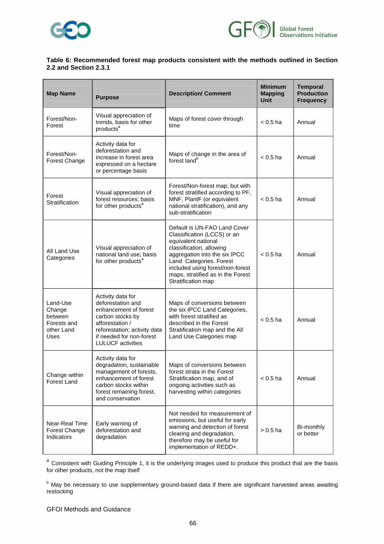
Table 6: Recommended forest map products consistent with the methods outlined in Section 2.2 and Section 2.3.1
Map Name
Purpose Description/ Comment
Minimum Mapping Unit
Temporal Production Frequency
Forest/Non-Forest
Visual appreciation of trends, basis for other productsa
Maps of forest cover through time
< 0.5 ha Annual
Forest/Non-Forest Change
Activity data for deforestation and increase in forest area expressed on a hectare or percentage basis
Maps of change in the area of forest landb
< 0.5 ha Annual
Forest Stratification
Visual appreciation of forest resources; basis for other productsa
Forest/Non-forest map, but with forest stratified according to PF, MNF, PlantF (or equivalent national stratification), and any sub-stratification
< 0.5 ha Annual
All Land Use Categories
Visual appreciation of national land use; basis for other productsa
Default is UN-FAO Land Cover Classification (LCCS) or an equivalent national classification, allowing aggregation into the six IPCC Land Categories. Forest included using forest/non-forest maps, stratified as in the Forest Stratification map
< 0.5 ha Annual
Land-Use Change between Forests and other Land Uses
Activity data for deforestation and enhancement of forest carbon stocks by afforestation / reforestation; activity data if needed for non-forest LULUCF activities
Maps of conversions between the six IPCC Land Categories, with forest stratified as described in the Forest Stratification map and the All Land Use Categories map
< 0.5 ha Annual
Change within Forest Land
Activity data for degradation, sustainable management of forests, enhancement of forest carbon stocks within forest remaining forest, and conservation
Maps of conversions between forest strata in the Forest Stratification map, and of ongoing activities such as harvesting within categories
< 0.5 ha Annual
Near-Real Time Forest Change Indicators
Early warning of deforestation and degradation
Not needed for measurement of emissions, but useful for early warning and detection of forest clearing and degradation, therefore may be useful for implementation of REDD+.
> 0.5 ha Bi-monthly or better
a Consistent with Guiding Principle 1, it is the underlying images used to produce this product that are the basis for other products, not the map itself
b May be necessary to use supplementary ground-based data if there are significant harvested areas awaiting restocking
GFOI Methods and Guidance
66
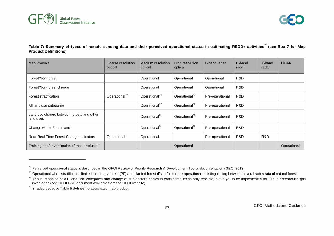
Table 7: Summary of types of remote sensing data and their perceived operational status in estimating REDD+ activities75 (see Box 7 for Map Product Definitions)
Map Product Coarse resolution optical
Medium resolution optical
High resolution optical
L-band radar C-band radar
X-band radar
LiDAR
Forest/Non-forest Operational Operational Operational R&D
Forest/Non-forest change Operational Operational Operational R&D
Forest stratification Operational77 Operational76 Operational77 Pre-operational R&D
All land use categories Operational77 Operational78 Pre-operational R&D
Land use change between forests and other land uses
Operational79 Operational79 Pre-operational R&D
Change within Forest land Operational78 Operational78 Pre-operational R&D
Near-Real Time Forest Change Indicators Operational Operational Pre-operational R&D R&D
Training and/or verification of map products78 Operational Operational
75 Perceived operational status is described in the GFOI Review of Priority Research & Development Topics documentation (GEO, 2013). 76 Operational when stratification limited to primary forest (PF) and planted forest (PlantF), but pre-operational if distinguishing between several sub-strata of natural forest. 77 Annual mapping of All Land Use categories and change at sub-hectare scales is considered technically feasible, but is yet to be implemented for use in greenhouse gas
inventories (see GFOI R&D document available from the GFOI website) 78 Shaded because Table 5 defines no associated map product.
GFOI Methods and Guidance
67
Box7: Map Definitions
Forest/Non-forest. This map shows the extent of all forests types meeting the national definition within a country. It may be necessary to supplement remote sensing with ground-based data obtained through the NFMS to help define forest areas subject to harvest which are temporarily unstocked. The map will be of use for visual appreciation of the extent of forest land, and the underlying data sets used to produce it will be the basis for subsequent products.
Forest/Non-forest change This map should be produced by analysis of the data which underlie the Forest/Non-forest product. It can be used to express increases or decreases in forest area relative to other land uses. The latter is deforestation expressed in area or percentage units. It is not yet deforestation expressed as greenhouse gas emissions, because the forest areas are not yet stratified into forest type, and hence carbon densities are unassigned.
Forest Stratification. The forest category within the land use category map will serve as a basis for stratification of forest. The aim of the stratification is to achieve relatively little variation in biomass density within a stratum to increase sampling efficiency lead to more accurate estimates. The primary stratification suggested by the FAO FRA is primary forest (PF), modified natural forest (MNF), and planted forest (PlantF). Countries may also use established national stratifications. Further stratification based on relevant forest types and classes may be necessary. Forest classes to be included vary between countries and ecoregions, including where applicable, regionally significant types such as peat swamp forest, mangrove, low-density forest. Likelihood of disturbance and secondary forest and regrowth can also be the basis for stratification. Remote sensing may help by detecting the source or indicators of human activity that can lead to degradation including logging roads, signs of canopy change, fires, or proximity to agricultural activity or infrastructure. Stratification implies more refined mapping and is needed to reflect differences in growth, carbon stocks and emissions/removals factors. In order to estimate the carbon losses associated with deforestation and degradation, the carbon densities of the forest before and after disturbance needs to be known. Stratification is therefore also the basis for collecting carbon densities by field measurements.
All Land Use Categories. This map product is required as a basis for the other products for national baseline mapping. Countries themselves decide what level of detail or classification scheme they wish to use, but should consider using the UN-FAO Land Cover Classification System (LCCS)79 to label the various identified land cover classes. Forest land is land used for forest consistent with the national definition (see Chapter 1). For emissions and removals reporting purposes, the classification system and digital maps should allow for aggregation of relevant classes into the main six IPCC Land Categories defined in the IPCC Good Practice Guidelines (Forest Land, Cropland, Grassland, Wetlands, Settlements and Other Land). Further division of the Forest Land category into forest types may be necessary for stratification to improve accuracy. This is likely to require ground based knowledge on forest types that can then be used to map, for instance, natural and planted forests, as well differentiate between forest age or forest types with different carbon stock levels.
Land Use Change between Forest and Other Land Uses. To calculate emissions and removals from deforestation or increases in forest area using the gain-loss method, countries need activity data. Most activity data are areas sufficiently disaggregated so that they can be used to estimate emissions or removals when combined with emission and removal factors and other parameters which are usually expressed per unit area. The map should contain categories of Forest Land converted to one of the other land categories (Cropland/Grassland/ Wetland/Settlements/Other Land), making five change categories and conversion of Cropland/Grassland Wetland/Settlements/Other Land to Forest Land another five change categories. This map may also contain categories of stable land covers. If spatial data collected by local communities on areas of land-use conversion exist, these should be incorporated into the conversion map. Consistent with Guiding Principle 2 described in Section 3.6, the conversion map is preferably created by the analysis of a time series of satellite imagery that is as long as possible. This is because an image pair is unlikely to provide sufficient information to separate between the different conversions and between land-use change and land-cover change.
Changes within Forest Land As described in Section 2.2.2, degradation in practice entails long-term loss of forest carbon stocks. Degradation or enhancement processes can be estimated through a combination of transitions between strata having different carbon densities. Ground-based data are used to estimate the carbon density within given strata. Degradation mapping may therefore be achieved by a combination of remote sensing (to detect signs of disturbance and hence indicate the extent of the potentially degraded area) and ground-based data (to detect the effect on carbon stocks). Estimation of degradation of forest carbon stocks directly by remote sensing alone is not currently possible80.
Near-Real Time Forest Change Indicators (Early Warning). This product is not required for UNFCCC REDD+ reporting, but is useful for early warning and detection of potential and actual changes in forest cover or
79 See http://www.fao.org/docrep/003/x0596e/x0596e00.htm 80 Research underway may lead to direct detection of degradation using radar data or shifts in spectral indices.
GFOI Methods and Guidance
68

degradation. Coarse resolution, frequent measurements are required for this purpose (e.g., MODIS, PALSAR ScanSAR).
3.5 Methods for mapping activity data
Factors that influence a country’s decisions concerning which data and methods to use for mapping activity data include the nature of the forests in the country, forest management practices, availability of various kinds of satellite data, existing satellite image analysis capabilities, availability of ground-based data and general level of technological capacity. Guiding principles given at the end of the section discuss aspects that may help a country decide on the combination of data sources and methods used to support reporting on GHG emissions and removals.
3.5.1 Maps of forest/Non-forest, Land Use, or Forest Stratification
At the heart of the use of remote sensing images is the translation of the remotely sensed measurements into information about surface conditions. Generating the various kinds of activity data necessary for estimating GHG emissions and removals involves categorization. For example, for estimation of forest area, a map is usually made that includes the categories forest and non-forest. Italics are used here to indicate names of categories (also called classes) in a map. To correspond to the top-level categorization adopted by IPCC GPG2003, a Land Cover map would need to have at least the following categories: Forest Land, Cropland, Grassland, Wetlands, Settlements and Other Land. There may be need to stratify forest areas according to ecosystem types or other categories that minimize the variability in carbon content. Consequently, methods that define categories, or classes, using remote sensing are particularly relevant. Collectively, these methods are referred to as image classification, and there is a long history of their use in remote sensing. There has also been extensive research on the best methods for image classification and as a result a wide variety of choices are available. Most image processing packages include several algorithms for image classification. Common image classification algorithms include maximum likelihood, decision trees, support vector machines and neural networks. Many of these are available in standard image processing software packages.
Image classification begins with the definition of the categories or classes to be included in the map. In supervised classification, it is necessary to provide training samples of each of the classes to be included. These samples could come from a variety of sources, including sample sites from an NFI, or could be obtained from high resolution images. For the simple classes of forest/non-forest, or the small number of top-level categories used by IPCC GPG, examples can often easily be found in the images being classified. Often images from a single date are used for image classification. However, multiple images from different seasons can also be used in image classification to try to capture classes with seasonal dynamics. As the level of stratification of forests increases, alternative sources of reference data to train classifiers will be needed, such as prior vegetation maps or field plots.
Classification can be done by visual interpretation, but this can be very human resource intensive because the number of pixels may be very large and interpretations can vary due to human judgement. This may be overcome by using automated algorithms in either non-supervised or supervised approaches to give results consistent with human interpreters in
GFOI Methods and Guidance
69

allocating a pixel to one forest type or another, or to segment the data. Non-supervised approaches use classification algorithms to assign image pixels into one of a number of unlabelled class groupings. Expert image interpreters then assign each of the groupings of pixels a value corresponding to the desired land class. Supervised approaches use expertly-defined areas of known vegetation types to tune the parameters of classification algorithms which then automatically identify and label areas similar to the input training data. The approaches have different challenges which are best addressed by iterative trials: supervised classification may wish to use more classes than are statistically separable; unsupervised methods may generate fewer classes than are desired and a given cover type may be split between several groupings. In both cases human interpreters can check whether the results of applying the algorithm appear reasonable in terms of the forest type distribution expected from prior information, and result in the absence of unlikely features. The relative advantage depends on whether the time taken in checking automatic classifications exceeds the time taken to achieve consistent results by relying entirely on human interpreters81.
Rarely does the first attempt at image classification result in the final map. Close examination of the classification results often reveals issues and problems that can be resolved by changes in the classification process. There are many ways to try to improve the results of a classification with noticeable problems, including the addition of more or improved training data. It may also be helpful to include additional kinds of data in the classification, such as topographic or climatic data.
Recognition of various strata of modified natural forests will generally need to take account of surrounding pixels because features such as crown cover disturbance, fragmentation or logging infrastructure will not occur in every pixel of the area affected. Consequently, when considering the boundary between modified natural forest and primary forest it will be necessary to establish a radius within which evidence for modification is taken to be relevant to the pixel in question. If pixel based classification is to be used subsequently the radius is used directly; if the pixels are first to be segmented (grouped according to common properties) it becomes an input to the segmentation process (see Box 8 below on Pixel and Object-based methods, and Segmentation).
Conceptually this radius is the distance needed to regain the characteristics of primary forest, represented for REDD+ purposes. A default of 500 metres can be used, but the value will depend on forest ecosystem and type of modification, and is best established by measurement82, especially if using an IPCC Tier 2 or 3 method. If the result of using a particular radius of influence is that fragments of nominally primary forest appear along the boundary between primary and modified natural forest, then the radius of influence being used is probably too small. This is because forest within a fragmented landscape is more likely to be modified than primary. Having established image characteristics of forest types and the radius of influence it is possible to assign a forest type (and sub-strata) to each pixel for the entire forest area of the country, as described above.
81 See Section 2.1 of the GOFC-GOLD sourcebook (GOFC-GOLD, 2012). 82 For example, work in Guyana using change metrics indicated that almost all the degradation associated with
new infrastructure occurs within a buffer zone about 100 metres deep (Winrock International, February 2012).
GFOI Methods and Guidance
70

Box 8: Pixel and Object-Based Methods and Segmentation
Acceptable accuracies for land cover and land cover changes can be achieved using either pixel-based or object-based classification methods. Object-based methods first group together pixels with common characteristics, a process called segmentation. At medium resolution as defined here these can sometimes yield higher overall accuracies than pixel-based methods for land cover classificationa. Segmentation is also useful for reducing speckle noise in radar images prior to classification. However if the smallest number of pixels to be grouped (the minimum mapping unit) is too large there is a risk of biasing the classification results. In practice this means that the minimum mapping unit should not exceed the smallest object discernible in the imagery. Image segments provide an advantage when part of a processing chain requires human interpreter input. This is because image segments can be combined into larger polygons which can be more easily reviewed and revised for classification errors (FAO & JRC, 2012)b. Tracking change at the pixel level opens the way to better representation of carbon pool dynamics, however it requires significantly more data processing.
Pixel-based approaches are potentially most useful where there are multiple changes in land use within a short period (for example, 10-15 year reclearing cycles). They are most suited when there is complete data coverage (sometimes referred to as wall-to-wall), and require methods to ensure time series consistency at the pixel level. The approach may also be applied to sample based methods where pixel-level time series consistency methods are used, with the results scaled up based on the sample size. The results may still be summarised in land use change matrices. In fact the method is equivalent to matrix representation at the pixel levelc.
In addition to the general principles of consistent representation of land when using remote sensing for representing land or tracking units of land using a pixel approach, MGD advice is that:
1. Once a pixel is included, then it should continue to be tracked for all time. This will prevent the double counting of activities in the inventory and will also make emissions estimates more accurate.
2. Stocks may be attributed to pixels, but only change in stocks and consequent emissions and removals are reported. This is to prevent large false emissions and removals as land moves between categories.
3. Tracking must be able to distinguish both land cover changes that are land-use changes, and land cover changes that lead to emissions within a land-use category. This prevents incorrect allocation of lands and incorrect emissions or removals factors or models being applied that could bias results.
4. Rules are needed to ensure consistent classification by eliminating oscillation of pixels between land uses when close to the definition limits
5. Consistency between inventory estimates and projections of future emissions and/or removals is challenging because rules must be developed that apply at the pixel level.
References: a See Yan Gao and Jean Francois Mas , 2008. A Comparison of the Performance of Pixel Based and Object Based Classifications over Images with Various Spatial Resolutions. Online Journal of Earth Sciences, 2: 27-35. b See http://www.fao.org/docrep/017/i3110e/i3110e.pdf
C Australian Greenhouse Office (AGO), 2002
3.5.2 Maps of change
To be consistent with IPCC guidance the Land Use Transition Map is composed of categories showing change. At the top level this includes conversion of Forest to Cropland or Grassland or Settlements or Wetlands or Other Land and vice versa. To make such a map, images are used from multiple dates and the change between dates is used to identify change. Change detection is one of the most common uses of remote sensing, and there are many methods that have been used, tested and proposed in the literature, although there is little information about which methods work best in which situations. In general, at least two dates of images (end-points) are necessary to map change. any methods use the change in a spectral band, bands or indices as the basis of the change detection process
GFOI Methods and Guidance
71

(Lambin and Strahler, 1994). Image classification methods are commonly used, in which case multiple images are used to make the assignment to stable classes (places that have not changed) as well as change classes (like Forest to Grassland). (Woodcock et al. 2001).
The GOFC-GOLD Sourcebook includes descriptions and examples of several change detection methods for monitoring deforestation 83 . It can be a useful resource when considering options for combinations of methods and remote sensing data to be used for mapping change.
More recently, methods that use many images, or a time-series of images, have been developed and tested (Chen, et al., 2004, Kennedy, et al., 2007, Furby, et al., 2008, Zhuravleva et al., 2013). These approaches have many advantages, as they are not so dependent on the conditions at the time the individual images were collected. As Guiding Principle 2 (see Section 3.6) indicates, the use of a time-series of images can help avoid some kinds of errors in the monitoring of forest change.
Georeferenced areas of forest planted annually or allowed to regenerate naturally within managed forest (Row 5 in Table 4) should be obtained from national forest authorities and stakeholders via the NFMS, and the existence of planted or regenerating forest on these areas confirmed as the appearance of the corresponding pixels merges with the appearance of other pixels with this forest type. This also applies to areas which may have the appearance of deforestation but which have in fact been subject to natural disturbance such as wildfires, cyclones, or pest outbreaks. Use of local information such as forest type and management intent, climatic extremes such as drought, and records of natural disturbance will be useful in aiding the translation of imagery into reliable activity data.
The mapped forest type and change areas (‘counted pixels’) produced using the methods described in section 3.5 will be biased because of classification errors. This can be estimated and corrected for using a sample of reference observations as explained in Section 3.7.
3.5.3 Maps of forest degradation
The methods described in Section 2.2.2 for estimating GHG emissions and removals associated with degradation require stratification (or categorization) of forests into primary, modified natural forest, and planted, or another stratification used by a country. There may be sub-stratification to capture different forest ecosystems or types of human intervention. Remote sensing can therefore play a significant role in assessing the impact of forest degradation through identifying the extent of strata and sub-strata and as a basis for selecting samples. In this approach, for the gain-loss method the remote sensing provides the activity data (areas) of Forest Land that have been degraded. Field samples are then used to assign emission and removal factors for the different map classes. Stratification using remote sensing can also be used in the design of sampling strategies for the stock change approach. Methods to use remote sensing to identify areas that have undergone degradation or other change include use spectral indices (combinations of spectral bands designed to accentuate surface characteristics), spectral mixture analysis, and textural analysis. Visual methods can also be effective for stratifying forests on the basis of
83 See Section 2.1 and 2.2 of the GOFC-GOLD, 2012. In particular Table 2.1.3 lists the main analysis methods for medium resolution imagery.
GFOI Methods and Guidance
72

degradation. Examples of identifying degraded forest areas can be found in Winrock International 2012, Souza et al 201384, and Bryan et al 201385.
3.6 Guiding principles for remote sensing data sources and methods
The following guiding principles are suggested to help countries decide on the combination of data sources and methods used to support reporting on GHG emissions and removals:
Guiding Principle 1: To find change, compare images, not maps
When mapping forest change, it is generally more accurate to find change by comparing images as opposed to comparing maps estimated from images.
It is natural to expect that - given two maps of the same area made at different times - one could find change by simply comparing the maps. However, that approach is prone to inaccuracy and can be misleading (Fuller, et al., 2003). The crux of the problem is that errors in the individual maps lead to the identification of false changes, that is, areas that appear to have changed when in fact they have not. A map is therefore best regarded as the end product of analysis of images. Maps may summarize change, and be used as activity data, but new change analysis should be based on the underlying images.
A simple example may help illustrate the problem. If a forest/non-forest map is 95% accurate (a level of accuracy that is very difficult to achieve in many environments where gradients for forest cover and density occur) is compared with a similar map for the same place at a later date with the same level of accuracy, if the errors in the two maps are assumed to be independent, then the expected accuracy of the map resulting from their comparison would be the product of the two, or approximately 90.25%. If the maps are correlated the accuracy will be better. In general, 90% is a very high level of accuracy for maps estimated from remote sensing. However, it is not sufficient accuracy for estimating the area of forest change annually in most parts of the world as the magnitude of change in most instances will be less than the cumulative error of the individual map products. To provide some perspective, the FAO Forest Resource Assessment defines “rapid deforestation” as the loss of more than 0.5% forest per year.
84 http://www.mdpi.com/2072-4292/5/11/5493; see also http://www.obt.inpe.br/degrad/
85 http://www.plosone.org/article/info%3Adoi%2F10.1371%2Fjournal.pone.0069679#s1
GFOI Methods and Guidance
73

Guiding Principle 2: Time Series Analysis and Consistency
When data are available from many time-steps, it is better to use the information from the entire time series of images rather than comparing only the end-dates.
This is especially important for reconstructing forest history since the time series can be used to reduce the reporting of unlikely land use changes (for example a conversion from non-forest → forest → non-forest within a time frame less than a forest growth cycle) which would not be revealed by comparing only two dates. By studying temporal trends, it is also possible to detect longer-term processes than can be achieved through two-date change analysis.
Consistent representation of lands is a key component of any greenhouse gas inventory (GPG2003, 2006GL) and aims to:
• Prevent omission of lands affected by activities;
• Prevent double counting of lands;
• Correctly allocate land to differing land uses; and,
• Minimise bias in emissions estimation.
Where remotely sensed imagery is used to identify the geographical extent of management activities, care should be taken to ensure that geographic boundaries are mapped consistently through time.
In order to do this it is necessary to ensure that:
• Imagery is accurately georeferenced and orthorectified using a digital elevation mode 86 so that spurious change is not identified during change detection processes, as a result of image misalignment.
• Improvements in the mapping of geographic boundaries due to the improved resolution of newer satellite sensors are back-corrected into older land use maps derived from lower resolution imagery.
86 To take account of significant variations is slope and elevation within the area
GFOI Methods and Guidance
74

Box 9: Maintaining time series consistency in activity data derived from remotely sensed imagery
Consistency requires that estimates are comparable over time. In the case of REDD+ this will mean that current and future annual estimates will need to be compared to a reference level determined from historic estimates. This requirement for a consistent time series of data over many years is crucial as in implementing REDD+ and determining its success, countries will need to show a long-term reduction in emissions.
Guyana has opted for a stratified random sampling approach combined with wall-to-wall mapping based on classification of 30 m resolution Landsat imagery for historical periods (to set baselines) and 5 m resolution RapidEye for on-going monitoring. A characteristic of the Guyana MRV is that these datasets are considered necessary in order to meet both the forest definition, the reporting requirements and broader goals of the MRV.
Multi-year time series optical data are required for the generation of the IPCC Land Category Transition Conversion products. Approaches to change detection and multi-temporal analyses are reasonably well established, but with the opening up of the Landsat archive, novel methods of utilising the extensive time series are required.
National operational examples
Australia’s NCAS: Country-wide land cover change maps are produced routinely using the Landsat archive (Furby, et al 2008). The high co-registration accuracy and radiometric consistency makes it possible to drill through the time series and evaluate land cover change on a pixel-by-pixel basis. Continuous improvement is anticipated as new data becomes available (e.g., high resolution DEMs and hyperspectral data) and methods for their integration are developed.
New Zealand utilised Landsat 30m imagery between 1990 and 2008 in the development of its National Forest Inventory. Between 2010 and 2011, 54 new scenes of SPOT-5 satellite imagery were acquired over four priority areas across New Zealand. As a result of the resolution change the geographical extent of forest area mapped between 1990 and 2008 from Landsat 30m resolution satellite imagery area appeared to be larger in some cases than the same area mapped in 2008 from SPOT 10m resolution imagery.
Where the true forest extent is unchanged, it is good practice to correct the mapping of the forest at 1990 based on the improved boundary delineation in the 2008 imagery.
GFOI Methods and Guidance
75

Box 10: Use of a combination of datasets to ensure continuity
Medium resolution optical data are currently the primary data source for monitoring forest cover change in the tropics (De Sy et al, 2012). Use of a consistent time series of observations is critical to obtain accurate results for assessing longer term forest area change (DeFries, et al. 2007; Verbesselt, et al. 2010; Achard, et al., 2010; GOFC-GOLD, 2012).
Optical data can be used stand-alone if cloud-free coverage is obtained. Time series, multi-year coverage is preferable. The scale and rate of change in forest cover affects its detection using optical satellite data. Obvious changes in forest extent due to clearing or conversion to other land uses can be detected using time series observations from medium (e.g., Landsat, SPOT-5) to coarse (e.g., MODIS) resolution optical data. Bi-annual and annual observation of change is possible over long time-scales. Coarse resolution data can also be used to locate hot spots for more detailed analysis using high resolution data. More subtle changes in forest cover require more frequent coverage at finer resolution (e.g., Quickbird, RapidEye). Fine resolution data are also useful for early detection of forest cover change and validation of results. The high cost of data and narrow coverage is limiting however (De Sy et al, 2012). A NFMS will probably need a combination of datasets to ensure continuity of coverage.
National operational programs
National operational programs utilising GFOI core (Landsat, CBERS) and non-core (IRS, MODIS) optical remote sensing data for forest cover change monitoring exist in Brazil (PRODES) - http://www.obt.inpe.br/prodes/index.php , Australia (NCAS) (Lehmann, et al., 2013, Furby, et al., 2008) and India (National Forest Cover MappingFI) (Pandey, 2008).
Amazon Monitoring Program, INPE: This is a world-leading example of operational, regional monitoring of tropical forests. Segmentation and unsupervised classification of time series Landsat, DMC and CBERS-2 imagery are used to estimate annual deforestation rates (Souza, 2006). A minimum mapping unit of 6.25 ha is applied. The approach could be improved by including degraded forest classes, explicit quantification of accuracy, better delineation of forest/non-forest boundaries, and future integration of SAR (cloud and smoke-penetrating) and CBERS-4 (high resolution and frequent coverage) data. INPE developed the open source TerraAmazon software for manipulation of multi-scale satellite data for deforestation monitoring.
The integration of various combinations of optical and SAR data can improve mapping of land use and land-use change. Interoperability in this case refers to the use of multi-scale optical data, multi-frequency radar data, and SAR-optical integration for improved land use and land-use change mapping. The latter exploits the texture and polarimetry of radar and unique spectral response in optical data for greater class separability and hence more accurate detection of change.
Guiding Principle 3: Always assess results from remote sensing.
The goal of the remote sensing analysis is to estimate the areas of the classes in activity data (for the gain-loss method) or provide information that can be used to guide sampling strategies (for the stock change method). There are multiple ways to do this. The apparently simple way to use the areas indicated in the maps as the final area estimate should not be done. The assignment to classes should first be subjected to rigorous assessment to correct biases in the area estimates and allow uncertainty characterization. Section 3.7 describes how, using reference data, to assess the accuracy, adjust for biases in area estimates and quantify uncertainty in area estimates. Reference data used for this purpose may be ground data or finer resolution or more accurately classified remotely sensed data. Accurate co-registration is needed or large errors may be introduced.
Guiding Principle 4: Document and archive the steps taken
To ensure transparency the data sets and analyses used for estimating greenhouse gas emissions and removals associated with REDD+ activities should be documented and archived, the aim being that a third party should understand, and if needed be able to repeat the steps taken. The information should include the imagery used, the types of pre-processing applied, the methods by which co-registration was achieved, the image classification methods used and the approach to statistical inference.
GFOI Methods and Guidance
76

3.7 Area, uncertainties and statistical inference for activity data
The IPCC definition of good practice requires that emissions inventories should satisfy two criteria: (1) neither over- nor under-estimates so far as can be judged, and (2) uncertainties reduced as far as is practicable (Penman et al., 2003). To satisfy these criteria, compensation should be made for classification errors when estimating activity areas from maps and uncertainties should be estimated using robust and statistically rigorous methods. The primary means of estimating accuracies, compensating for classification errors, and estimating uncertainty is via comparisons of map classifications and reference observations for an accuracy assessment sample.
Factors that affect satisfaction of the two criteria are the sampling design and sample size for the accuracy assessment sample and map accuracy. For accuracy assessment and estimation to be valid for an area of interest using the familiar design- or probability-based framework (McRoberts, 2014), the reference data must be collected using a probability sampling design, regardless of how the training data are collected. The most common probability sampling designs are simple random, systematic, stratified random (simple random sampling within strata), and stratified systematic sampling (systematic sampling within strata). A key issue when selecting a sampling design is that the sample size for each activity must be large enough to produce sufficiently precise estimates of the area of the activity. Simple random and systematic sampling designs produce samples sizes for individual activities that are approximately proportional to their occurrence. If a very large overall sample is obtained, then simple random or systematic sampling may produce large enough sample sizes for individual activities to produce estimates of sufficient precision. However, unless the overall sample size is large, sample sizes for activities representing small proportions of the total area may be too small to satisfy the precision criterion. Thus, given the likely rarity of some activities and the large costs associated with large samples, serious consideration should be given to stratified sampling for which the strata correspond to map activity classes.
The success of any sampling design depends on map accuracy as reflected by the degree to which the predicted activities (map classes) correspond to the actual activities (reference observations) at each location. Map accuracy assessments are often summarized in the form of error or confusion matrices that summarize results and facilitate estimation of accuracies, activity areas, and uncertainties. Although an error matrix does not directly provide estimates of activity areas or their uncertainties, the information in an error matrix can be used to do so (McRoberts & Walters, 2012; Olofsson et al., 2013). Of crucial importance, large overall map accuracies do not guarantee accurate and precise estimates of individual activity areas.
Two general approaches to constructing change maps may be considered: direct classification entails construction of the map directly from a set of change training data and two or more sets of remotely sensed data, whereas post-classification entails construction of the map by comparing two or more separate land cover maps, each constructed using single sets of land cover training data and remotely sensed data. Although direct classification is often preferred, post-classification may be the only alternative because of factors such as the inability to observe the same sample locations on two occasions, insufficient numbers of change training observations, or a requirement to use an historical baseline map. The nature
GFOI Methods and Guidance
77

of the reference data necessary for estimation of activity areas from change maps depends on the method used to construct the map. For maps constructed using direct classification, the reference data must consist of observations of change based on land cover observations for two dates for the same sample locations. For maps constructed using post-classification, reference data may consist of either the same reference data as for maps constructed using direct classification or land cover observations for two dates, each at different locations. For the latter reference data, change cannot be estimated directly, but rather the extent of land cover is estimated for each date, and change is estimated as the difference between the two estimates (Coppin et al., 2004; McRoberts & Walters, 2012; McRoberts, 2014). Regardless of the accuracy assessment and estimation approach used, the estimators (statistical formulae) used for calculating estimates must correspond to the accuracy assessment sampling design.
Reference observations may be acquired from several sources, but their quality should be greater than the quality of the map data and the data used to construct the map. Although ground data acquired by field crews that can be accurately co-registered to the map are generally regarded as the standard, finer resolution remotely sensed data and more accurately classified remotely sensed data have also been used (Stehman, 2009, Sannier et al., 2014).
Two examples illustrate methods for estimation of activity areas, one based on a stratification approach (Cochran, 1977; Olofsson et al., 2013) and the other based on a model-assisted approach (Särndal et al., 1992; Sannier et al., 2014). The stratified approach illustrated in Example 1 uses the discrete classes of a response variable to assign pixels to change categories constituting strata. This approach is particularly useful when the strata correspond to activities and when large numbers of reference observations are available for each activity. However, area estimation may also be accomplished using sampling units larger than single map pixels such as when the reference data are obtained from very high resolution imagery. The model-assisted approach of Example 2 is particularly useful when the response variable for these larger units is continuous and when the relationship between reference data and map data used as auxiliary information can be exploited to increase precision.
Example 1: A stratified approach to accuracy assessment and area estimation
Data and sampling design
A 30-m x 30-m Landsat-based change map for 2000 to 2010 consisted of two change classes and two non-change classes: (1) deforestation with area of 13,500 ha (2) forest gain with area of 28,800 ha, (3) stable forest with area of 6,450,000 ha, and (4) stable non-forest with area of 580,500 ha.
Because the areas of the map change classes are small, together comprising only 3.5% of the total area, a stratified random sampling design with the four map classes as strata was selected for acquiring an accuracy assessment sample. The sample size must be large enough to yield sufficiently precise estimates of the areas of classes but small enough to be manageable. An arbitrary sample size of 500 pixels was deemed manageable and was distributed with 75 pixels to each of the two change classes, 125 pixels to the stable forest class, and 225 pixels to the stable non-forest class.
GFOI Methods and Guidance
78

Estimation
The reference data consisted of manual classifications of the Landsat pixels selected for the sample. The same underlying Landsat data were used to produce both the map and reference classifications, albeit with the assumption based on three independent assessments that the reference classifications were of greater quality than the map classifications. An error matrix was constructed based on a pixel-by-pixel comparison of the map and reference classifications for the accuracy assessment sample (Table 7).
Table 8: Example 1 – Error matrix of sample counts
Reference
Defore-station
Forest gain
Stable forest
Stable non-forest
Total 𝐀𝐦,𝐢 [pixels] 𝐖𝐢
Map
Deforestation 66 0 5 4 75 200,000 0.020
Forest gain 0 55 8 12 75 150,000 0.015
Stable forest 1 0 117 7 125 3,200,000 0.320
Stable non-forest
2 1 9 213 225 6,450,000 0.645
Total 69 56 139 236 500 10,000,000 1.000
The cell entries of the error matrix are all based on the accuracy assessment sample. The sample-based estimator (statistical formula) for the area proportion, pij, is denoted as p�ij, where i denotes the row and j denotes the column in the error matrix. The specific form of the estimator depends on the sampling design. For equal probability sampling designs, including simple random and systematic designs, and stratified random sampling designs for which the strata correspond to the map classes, as is the case for this example,
p�ij = Winijni∙
, (3)
where Wi is the proportion of area mapped as class i (see the final column in Table 7) and ni∙ is nij summed over j. Accordingly, the error matrix may be expressed in terms of estimated area proportions, p�ij (Table 8), rather than in terms of sample counts, nij (Table 7).
GFOI Methods and Guidance
79

Table 9: Example 1 – The error matrix of estimated area proportions
Reference
Defore-station
Forest gain
Stable forest
Stable non-forest
Total (𝐖𝐢) 𝐀𝐦,𝐢 [pixels]
Map
Deforestation 0.0176 0.0000 0.0013 0.0011 0.020 200,000
Forest gain 0.0000 0.0110 0.0016 0.0024 0.015 150,000
Stable forest 0.0026 0.0000 0.2995 0.0179 0.320 3,200,000
Stable non-forest
0.0057 0.0029 0.0258 0.6106 0.645 6,450,000
Total 0.0259 0.0139 0.3283 0.6320 1.000 10,000,000
Once p�ij is estimated for each element of the error matrix, accuracies, activity areas and
standard errors of estimated areas can be estimated. User’s accuracy U�i = p�iip�i∙
, producer’s
accuracy P�j = p�jjp�∙j
, and overall accuracy O� = ∑ p�jjqj=1 , where q notes the number of classes,
are all estimated area proportions.
For this example, the estimate of user’s accuracy is 0.88 for deforestation, 0.73 for forest gain, 0.94 for stable forest, and 0.95 for stable non-forest. The estimate of producer’s accuracy is 0.68 for deforestation, 0.79 for forest gain, 0.91 for stable forest, and 0.97 for stable non-forest. The estimated overall accuracy is 0.94.
The estimated area proportions in Table 8 are then used to estimate the area of each class. The row totals of the error matrix in Table 8 are the mapped area proportions (Wi) while the column totals are the estimated area proportions based on the reference data. A stratified estimator of the area proportion for class j is,
p�∙j = ∑ Winijni∙i (4)
(Cochran, 1977, Equation 5.52). The area estimate for class j based on the reference data is calculated as the product of p�∙j and the total map area. For example, the estimated area of deforestation based on the reference data is A�1 = p�∙1 × Atot = 0.0259 × 10,000,000 pixels = 258,933 pixels = 23,304 ha. Thus, the mapped area of deforestation (Am,1) of 200,000 pixels (18,000 ha) is an underestimate by 58,933 pixels or 5,304 ha.
The next step is to estimate a confidence interval for the estimated area of each class. The standard error (SE) of the stratified estimator of estimated proportion of area (the column totals in Table 8) is estimated as,
SE�p�∙j� = �∑Wip�ij−p�ij
2
ni∙−1i (5)
GFOI Methods and Guidance
80
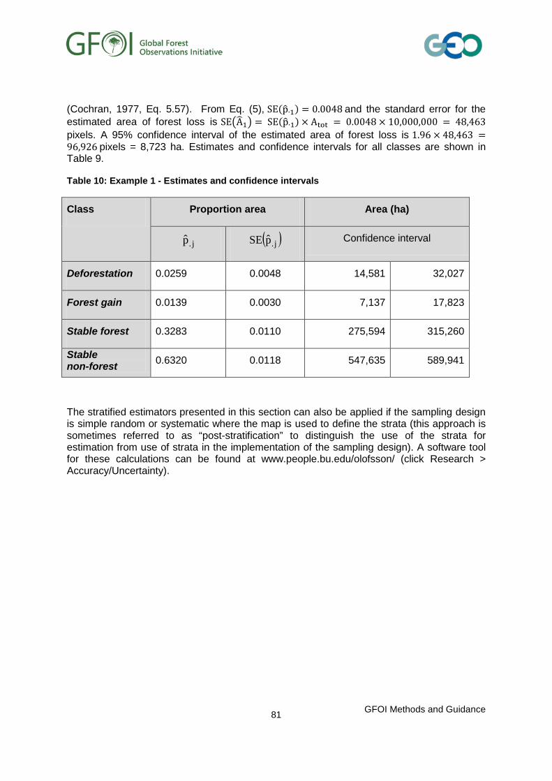
(Cochran, 1977, Eq. 5.57). From Eq. (5), SE(p�∙1) = 0.0048 and the standard error for the estimated area of forest loss is SE�A�1� = SE(p�∙1) × Atot = 0.0048 × 10,000,000 = 48,463 pixels. A 95% confidence interval of the estimated area of forest loss is 1.96 × 48,463 =96,926 pixels = 8,723 ha. Estimates and confidence intervals for all classes are shown in Table 9.
Table 10: Example 1 - Estimates and confidence intervals
Class Proportion area Area (ha)
j.p ( )j.pSE Confidence interval
Deforestation 0.0259 0.0048 14,581 32,027
Forest gain 0.0139 0.0030 7,137 17,823
Stable forest 0.3283 0.0110 275,594 315,260
Stable non-forest 0.6320 0.0118 547,635 589,941
The stratified estimators presented in this section can also be applied if the sampling design is simple random or systematic where the map is used to define the strata (this approach is sometimes referred to as “post-stratification” to distinguish the use of the strata for estimation from use of strata in the implementation of the sampling design). A software tool for these calculations can be found at www.people.bu.edu/olofsson/ (click Research > Accuracy/Uncertainty).
GFOI Methods and Guidance
81

Example 2: A model-assisted approach to accuracy assessment and area estimation
Data and sampling design
In Example 2, a 100,000-km2 region of a tropical country was divided into 20-km x 20-km blocks with each block further subdivided into 2-km x 2-km segments. A 30-m x 30-m, forest/non-forest classification was constructed for the entire region for each of 1990, 2000, and 2010 using Landsat imagery and an unsupervised classification algorithm. For each time interval, the map data for the ith segment consisted of the proportion of pixels, iy , whose classifications changed from forest to non-forest. Reference data were acquired for each year by randomly selecting one segment within each block and visually interpreting each pixel within the segment as forest or non-forest using independent Landsat data, aerial photography, and other spatial data. The sample of segments was denoted S, and for each time interval, the reference data for the ith segment consisted of the proportion of pixels, yi, whose visual interpretations changed from forest to non-forest.
Estimation
For each time interval, the map-based estimate of proportion deforestation area was,
∑==
M
1iimap y
M1p , (6)
where M=25,000 was the total number of segments in the study area. However, the map estimates are subject to classification errors which introduce bias into the estimation procedure. An adjustment term to compensate for this bias is,
( ) ( )∑∈
−=Si
iimap yym1pasiB , (7)
where m=250 is the number of segments in the sample. The adjusted estimate is the map estimate with the adjustment term subtracted,
( )mapmapadj pasiBpp −=
( )∑ ∑= ∈
−−=M
1i Siiii yy
m1y
M1 (8)
The standard error (SE) of adjp is,
SE�p�adj� = �Va�r�p�adj� = ( ) ( )∑∈
ε−ε− Si
2i1mm
1 (9)
Where ( )iii yy −=ε and ∑∈
ε=εSi
im1
.
GFOI Methods and Guidance
82

This estimator is based on an assumption of simple random sampling. For stratified sampling, as is the case for this example, variances and standard errors may be conservatively over-estimated. Estimates of deforestation area for each time interval are shown in Table 10.
Table 11: Example 2 - Regional estimates of deforestation area
Interval Estimate (proportion deforestation area) Confidence interval (km2)
mapp ( )mappasiB adjp ( )adjpSE Lower limit Upper limit
1990-2000 0.0017 0.0015 0.0033 0.0012 95 565
2000-2010 0.0003 0.0009 0.0011 0.0012 -125 345*
1990-2010 0.0020 0.0024 0.0044 0.0016 126 754
*Because the interval includes 0, the estimate of deforestation area was not statistically significantly different from 0.
In the statistical literature, these estimators are characterized as the model-assisted regression estimators even though prediction techniques other than regression may be used and the model may be implicit (Särndal et al., 1992; Section 6.5).
Summary of examples
An important distinction between the approaches illustrated in the two examples pertains to the use of the map data. In the first example, the pixel-level map data are in the form of discrete classes and are used only to construct strata, to calculate stratum weights, and to reduce the variance of the area estimate relative to the variance of the estimate based only on the reference observations. Of importance, with the stratified estimator for the first example, the within-stratum estimates are based entirely on the reference observations. In the second example, the map data are used as a continuous, segment-level, auxiliary variable. The model-assisted estimator facilitates greater exploitation of the relationship between the segment-level reference proportion of area and the segment-level map proportion of area. The results are that the model-assisted estimator requires compensation for the effects of segment-level model prediction error, but it also exerts a greater influence on the final estimates via a greater reduction in the variance error of the area estimate.
GFOI Methods and Guidance
83

3.8 Collection of ground observations and the derivation of emissions removal factors
Ground-based observations are an essential input to the estimation of emissions and removals. Useful data are often available through collections made for other purposes, such as monitoring of timber volume production or from scientific research. Although availability will differ from country to country, relevant ground-based observations may include:
• NFIs or sub-national forest inventories or assessments such as plot or transect measurements, growth and yield studies, harvested wood removals, and equations for converting these to biomass
• spatial maps of forest type, forest management, disturbance history, soil type and C content, land use
• research and operational data that can be used to estimate emissions and removals factors for C in biomass, dead organic matter and soils
• detailed measures which can be converted to emission factors for non-CO2 GHGs from soils and fire.
The ground data can be used to produce maps, emissions removals factors, growth models for different types of forest, or to parameterise models such as soil carbon models. These data may need to be stratified according to forest type, soil and climatic conditions, topography, and the nature of forest disturbances induced by management or natural factors. This is essential to ensure that the data are applied to relevant domains (strata) of the national forest.
The types of data collected and the methods used will vary widely. For example, to estimate non-CO2 emissions factors for biomass burning will require complex scientific methods and equipment, collecting further data on forest types to improve maps will require staff with specific skills and knowledge of how to identity forest types from the ground.
Although the existing data may not be in a readily usable form, it is likely to be much more cost effective to use existing data where possible, and in general it will be efficient for the NFMS to collate relevant existing information.
The NFMS should establish:
• REDD+ activities which are under consideration for including as national mitigation actions. This will generally be a matter of national policy.
• data required for estimating associated emissions and removals. Advice on this is set out in Chapter 2 of this document, in conjunction with the GPG2003. Key category analysis (see section 1.2) will help prioritize data needs
• what existing data sets there are to serve these needs, by contacting via the NFMS relevant Ministries, statistical agencies, academic institutions and stakeholders.
The NFMS should then collate the existing data and acquire new data where needed.
Because of synergies, it is likely to be cost effective to integrate an NFI, where one exists, into the NFMS; nevertheless cost-effective application of IPCC methods does not
GFOI Methods and Guidance
84

necessarily imply development of an NFI where one does not already exist. Figure 3 represents a decision tree to help decide this question.
3.9 Generic advice on use of ground observations to estimate change in carbon pools and non-CO2 GHG emissions
3.9.1 Biomass
Biomass carbon is usually a significant pool, and methods are required to estimate biomass carbon stocks and their change. For example, the gain-loss methods described in Section 2.1.2 require the following:
1. biomass carbon densities in primary forest, modified natural forest, and planted forest sub-stratified as required by forest type, and management regime or likelihood of disturbance
2. annual rates of change in biomass carbon density in modified natural forest sub-stratified as required by forest type and management regime or likelihood of disturbance
3. long-run average biomass carbon density and corresponding rates of change in planted forest sub-stratified as required by forest type and management regime or likelihood of disturbance.
The stratification into primary forest, modified natural forest, and planted forest is consistent with the FAO’s Global Forest Resource Assessment. Countries may use other stratifications according to national circumstances, e.g. if there is an established national stratification or if the use of an alternative stratification will reduce the number of sub-strata required.
3.9.1.1 Estimating biomass carbon from surrogate measures In practical terms, biomass needs to be estimated indirectly, often using allometric models which relate biomass to surrogate measurements, often trunk diameter and sometimes also height. These models are established using destructive sampling, but this is expensive and it is not practical to rely on direct measurements alone. Sources of uncertainty in estimating above-ground biomass in a forested landscape (or stratum of it) using surrogate measurements include (Chave, et al. 2004, Molto, et al. 2013):
• quality of the tree measurements made in forest inventories (diameters or heights)
• reliability of the allometric model selected to convert tree measurements to biomass
• size of the sampled area (plot)
• representativeness of the sampled plots of the broader forest landscape or strata adopted.
GFOI Methods and Guidance
85

Forest sampling using plots should be the basis for estimating biomass carbon density. Large plots are required where biomass distribution is spatially uneven (e.g. due to patchiness in tree distribution in dry or previously disturbed forests, or due to irregular distribution of large trees). There is a trade-off between plot size and sample size, but for example in tropical rainforest plots should be at least 0.25 ha in area (Chave, et al., 2004). Chave, et al. (2003) showed that to estimate above-ground biomass with an error of 20% with 95% confidence in rainforest in Panama required 26 plots of this area (50 m x 50 m), or 160 20 m x 20 m plots. Subsequent analysis (Chave, et al., 2004) suggested that as a generalization, provided that reliable allometric models are applied, the total area of forest sampled should be ~ 5 ha. Preliminary sampling should be conducted in each forest strata to guide the intensity of sampling required. Tools such as the CDM Calculation tool can be used to estimate an optimum number of plots for a required accuracy87.
Plots should be located using GPS and marked in the field, unless they are temporary (see below)88. As discussed in Section 5.3.3.2 of GPG2003, costs can be reduced by locating plots in small clusters of say 4 or 5, provided separation of plots within the cluster is sufficient to avoid major correlations. Nested plots, where small trees are only measured on a sub-set of the plot, are another way of reducing the cost of measurement at a point. Plot shape is not critical; square or circular may be convenient.
Where spatial variability is high, stratified sampling which takes advantage of remotely sensed or other spatial data may need to be applied to achieve desired levels of precision for fixed costs (See Box 4). For example, the use of stratification reflecting differences in forest type, age, or tree size distribution is likely to be much more efficient in reducing the uncertainty than simply increasing sample size. Different allometric models may be needed for each stratum, so the availability of appropriate allometric models can be a practical constraint on the number of forest strata used, and new allometric equations may need to be developed. Sufficient sampling may already available through an NFI, and the agency responsible for the NFI should be consulted via the NFMS about the relationship between NFI data and the proposed stratification, and the availability of suitable allometric models to estimate biomass for the purposes of REDD+ activities. This should be done before new field work is done or further stratification is decided.
The stem diameters of all trees that are at least half within the plot are measured and biomass established using appropriate allometric models. Generally tree diameters should be measured at least 130 cm above the ground and below the first branching point. The height chosen should be consistent with that used to develop the allometric model being used. It is important that the range of tree sizes used to develop the allometric model cover that encountered in the forest, because failure to sample adequately large trees (many trees may exceed 100 cm in diameter in tropical forests; Henry, et al., 2010) will result in very uncertain biomass estimates. Chave, et al. (2004) found that for tropical rainforest the coefficient of variation89 associated with the allometric model was ~ 20% when 20 trees were sampled to construct it, but that this declined to 10% when the sample size was ~50 trees. Although stem diameter is often an adequate biomass predictor, including height can reduce uncertainties significantly, although height is harder to measure (see Annex G, which has
87 The CDM tool for calculating the number of measurement sample plots is available from http://cdm.unfccc.int/methodologies/ARmethodologies/tools/ar-am-tool-03-v2.1.0.pdf/history_view
Whilst this tool is targeted at A/R projects the principles can be applied in other circumstances. 88 The GPS should be used in the location of the plot. More accurate techniques (i.e. compass and tapes) should
be used in defining the boundaries of the plot.
89 The standard deviation divided by the mean
GFOI Methods and Guidance
86

more detail on the derivation and application of allometric models). Countries are advised to use diameter, and height where it is feasible to do so. Countries should use equations that best represent their forest types and which are consistent with established and validated practice. Since changes in biomass also need to be estimated, the locations of plots should be generally permanent so that the trees in the same area can be re-sampled periodically.
Preferably allometric models should estimate below- as well as above-ground biomass, and be developed for relevant tree species and circumstances. FAO and CIRAD have published a manual on how to do this and a database of existing equations with information on the circumstances under which they apply 90 . For native forests, which may contain many different species, application of species-specific allometric models may be impractical, in which case non-species-specific, regionally relevant allometric models can be used (Chave et.al., 2004). Generic equations are based on large numbers of trees sampled across landscapes, and tend to be more reliable than locally developed equations if these are based on only a small number of trees (Chave, et al., 2005). Often allometrics are only available to estimate above-ground biomass, but below-ground biomass can be estimated using root-to-shoot ratios, default values are available from IPCC91, although this approach will increase uncertainties significantly.
Biomass densities should be multiplied by mass of carbon per mass of biomass to convert to carbon densities. The default ratio in the GPG2003 is 0.592. More specific figures for tree components and forest domains are given by IPCC93.
3.9.1.2 Estimating changes in biomass carbon densities The methods described in Section 2.2 require annual estimates of the change in biomass carbon density in modified natural forests and planted forests. This is calculated as the average over the permanent sample plots of differences between carbon densities at two points in time. Plots should be measured every 5-10 years and the rate of change estimated from the most recent pair of measurements, divided by the number of years separating them. Each plot will provide a rate of change. The estimated rate of change for the stratum is the weighted average of the individual plot rates of change and the uncertainty range at the 95% confidence interval94 can be estimated from their distribution about the mean.
Permanent plots, established in a systematic manner can be used to improve the accuracy of change estimation when repeatedly measured over time. However if these plots are treated in a way that is different from the rest of the forest (e.g. not harvested or thinned in the same way), or if the original population changes due to the removal of specific types of land without a corresponding removal of plots, the permanent plots will no longer be
90 The manual is at http://foris.fao.org/static/allometric/Manual_EN_WEB.pdf and the international associated
database for tree allometric equations at http://www.globallometree.org/ 91
Refer to 2006GL, Chapter 4; specifically Table 4.4. 92 The 2006 guidelines use 0.47. Countries should be consistent in the value they apply. 93 Refer to 2006GL, Chapter 4; specifically Table 4.3. Available from
http://www.ipcc-nggip.iges.or.jp/public/2006gl/pdf/4_Volume4/V4_04_Ch4_Forest_Land.pdf 94 The 95% confidence interval is commonly used by the IPCC guidance material.
GFOI Methods and Guidance
87

representative of the current forest. Remotely-sensed data, such as canopy cover or disturbance, may be used to determine whether the permanent plots have been treated in a non-representative fashion. If the permanent plots are no longer representative of the larger forest, then a new set of plots may be required to represent more accurately the current condition – this new set may be a temporary set of plots if the permanent plots can continue to produce reliable estimates of forest change for that area of forest that they represent. Alternatively, the permanent plots may be incorporated into a model-based approach which uses a remotely sensed variable in a model to relate accurately to current condition. Sampling with partial replacement systems where a proportion of permanent plots are replaced each measurement period have been used in the past as a compromise to estimating change and current condition, but have generally been found to be a complex compromise and difficult to maintain.
3.9.1.3 Estimating changes in long-run biomass carbon densities in planted forests Data on above ground biomass density at the point of final harvest (P), the time from replanting to harvest (t) and the average delay between final harvest and replanting (δt) for each type of plantation present (respectively P, t1 and δt in Box 5) should be obtained from stakeholders via the NFMS and used in the calculation described in Box 5. Values of P may be compared with above-ground biomass densities provided in GPG2003 for typical plantation types, using the values for greater than 20 years where separately provided. Since management practices may change over time, and growth rates are highly location-specific this is only an approximate check. Large differences should be discussed with stakeholders. Values of (t1+δt) may be checked using archived medium resolution remotely sensed data, since this is the time between harvests, which should be identifiable in imagery. Uncertainties in P and (t1+δt) should be obtained by analysing historical records (e.g. of the volume of wood removed at harvest) and expert judgement.
3.9.1.4 Remote sensing methods to support biomass estimation In addition to their use in the spatial mapping needed to estimate carbon stocks and changes, remotely sensed data can also contribute to estimating biomass density. They do not remove the need for ground estimates of biomass based on sample plots, but have the potential to complement them, especially where access is difficult or expensive, e.g. in mountainous areas.
Direct estimation of above-ground biomass (AGB) and change using remote-sensing is technically challenging. Annex F provides a brief review of the key issues and current capability, and concludes that existing biomass maps derived from remote sensing data should not be used unless extensive in-country testing is performed to confirm their reliability for application in specific forest types and at varying spatial scales.
Data acquired by SAR and LiDAR are currently the most promising technologies. SAR-based products have been demonstrated at sub-national (GEO, 2011; Mitchell et al, 2012)
and project (GEO, 2012; Englhart, et al., 2011; Williams, et al., 2009) levels, using data acquired by satellite (ALOS PALSAR, TerraSAR-X) and airborne (GeoSAR) data sources. Sensor interoperability for improved biomass estimation, and consistency in estimation across different vegetation types requires further research.
Airborne LiDAR has been used operationally (See Box 11 and Jochem, et.al., 2010). The basic assumption is that the mass of biomass is proportional to its volume, estimated by integrating over known area the difference in height between ground level taken from a digital terrain model, and the top of the canopy of individual trees measured by the time of return of a reflected light signal sent from an aircraft. The proportionality factor is likely to differ between the different strata and sub-strata being used and needs to be established
GFOI Methods and Guidance
88

empirically, hence the need for ground data to calibrate. The empirical relationships will reveal the uncertainties.
Box 11: LiDAR – Operational use in New Zealand and Research in Tanzania
New Zealand reports the use of airborne LiDAR, in combination with field measurements, to estimate changes in carbon stocks in forests planted after January 1st 1990. The New Zealand Land Use Carbon Accounting System (LUCAS) uses LiDAR imagery to measure the heights of trees and to characterise tree canopies. This has been calibrated with field measurements and modelling to determine the total amount of biomass carbon in plantation forest. An inventory of approximately 600 plots determined from a 4 km grid overlaid on all forests in New Zealand planted since 1990 are surveyed with LiDAR. The LiDAR data are calibrated against the field measurements for forest plots that are inaccessible. LiDAR data will be processed to provide the total amount of carbon per plot; the measurement process on the same plots will be repeated at the end of the Kyoto Protocol’s first commitment period. New Zealand reports this technique is cost effective in highly inaccessible forest areas.
For more detail see: http://www.mfe.govt.nz/publications/climate/looking-at-lucas/looking-at-lucas-issue-2.html
A Norwegian funded MRV research project in Tanzania encompasses a range of research activities that focus on LiDAR and emerging radar technologies and techniques. At the time of the project conception it was recognised that many of these technologies were evolving and had not been implemented operationally in MRV systems. However, the understanding was that the techniques developed would provide further research in these areas.
At the activity level, the acquisition of LiDAR was designed to test and document the accuracy of airborne LiDAR for estimating biomass and carbon stock change
LiDAR is an advanced technology that requires specialist knowledge (i.e. processing and model building) and is relatively untested in REDD+ countries.
However, there is a fairly high degree of sophistication associated with acquiring, processing and interpreting the results. The efficiency and subsequent utilisation of LiDAR technology can only occur if the national institutions have the expertise and capacity to carry out a similar level of analysis as being undertaken by Norwegian institutions.
For more detail see: http://www.norway.go.tz/News_and_events/Climate-Change/Mid-Term-Review-of-the-REDD-Research-Project-/#.Um3NchCzIvl
Wall-to-wall estimation of biomass using LiDAR may fill a niche in local projects within countries. Sample based approaches are favoured, in combination with coincident field plots and complete coverage SAR (ALOS PALSAR (Anderson et al, 2012, Siqueira et al, 2010) or optical (RapidEye (Kandel et al, 2013)) data, and is an active research topic. There is no satellite LiDAR currently in operation. Coarse vegetation height samples obtained from IceSAT GLAS (decommissioned) were combined with optical and SAR data to estimate AGB (GEO, 2012; Mitchard et al, 2012). The transferabillity of algorithms developed in boreal forest for biomass estimation in tropical forest needs further testing. A combination of sensors (optical-radar-LiDAR) and ground observations will probably be the best approach, but is currently still under research.
GFOI Methods and Guidance
89
3.9.2 Dead wood and litter pools
Gain-loss or stock change methods can be used for estimating the carbon stock changes in dead wood and litter. The choice of method for estimating DOM changes may be affected by the choice of method for biomass carbon stock change estimation. It is good practice that the stratification of Forest Land adopted for DOM should be the same as that used for the estimation of changes in biomass carbon stocks.
Apart from very generic information in Table 2.2 of Volume 4 of the 2006GL, IPCC does not provide default data on these pools, but they do contribute to emissions and removals associated with REDD+ activities. Estimated carbon stocks and stock change for these pools need to be obtained by sampling, ideally using the same sampling sites established for biomass estimation as described above. If methods for estimating these pools are not already established, e.g. via the NFI, countries are advised to apply the methods set out by the UNFCCC for use with afforestation and reforestation projects under the Clean Development Mechanism95. Uncertainties should be estimated from the variance around the mean of the spatial estimates.
3.9.3 Change in soil carbon stocks
It is usually impractical to monitor directly soil carbon change across diverse and extensive forest landscapes. Unless applicable country-specific soil carbon stock change (Tier 2) data are available96, for mineral soils countries are advised to use the Tier 1 method outlined by IPCC in Section 3.3.3.1 of GPG2003 97 for conversions to Cropland and in 3.4.1.2 for conversions to Grassland in order to estimate the effects of deforestation.
Developing a Tier 3 modelling approach for mineral soils is a major undertaking requiring considerable knowledge and data. The basic elements are:
• stratification by climatic zones, major forest types and management regimes coherent with those used for other C pools in the inventory, especially biomass
• determination of dominant soil types in each stratum
• characterization of corresponding soil C pools, identification of determinant processes in soil organic carbon input and output rates and the conditions under which these processes occur
• development and implementation of suitable models to estimate carbon stock changes for each stratum, including model evaluation procedures; and the establishment of benchmark sites where potential change in soil carbon stocks can be studied and used for model refinement. Models should be peer-reviewed, and
95 Estimation of carbon stocks and change in carbon stocks in dead wood and litter in A/R CDM project activities EB67 report, Annex 23, available at http://cdm.unfccc.int/methodologies/ARmethodologies/tools/ar-am-tool-12-v2.0.0.pdf
96 These methods may include complex models such as Century or RothC that determine the net difference
between rates of input of C to the soil as litter, and rates of C loss by decomposition. Research studies within countries would be needed to define the main factors (soil type, land transitions, and management practices) affecting emission and removal factors and to calibrate and test such models
97 Corresponding to Section 2.3.3.1 in Volume 4 of the 2006GL
GFOI Methods and Guidance
90

validated with independent observations representative of the ecosystems under study.
Background on soil monitoring is available in the scientific literature (Kimble et al., 2003, Lal et al., 2001, McKenzie et al., 2000).
IPCC sources of emission factors for activities on organic soils are listed in Section 2.2.4, Table 3 above. The uncertainty ranges are large, but manageable provided the coefficients are used consistently and do not change over time. In drained tropical peat soils fire can result in large, and spatially and temporally highly variable GHG emissions which are the combination of both CO2 and non-CO2 gases. The IPCC Wetlands supplement provides the most recent guidance on estimating GHG emissions from fires burning organic soils. Default emission factors for calculating such emissions are found in Chapter 2, Table 2.6 and Table 2.7.
Non-CO2 emissions factors for fires on peatlands are discussed in Section 3.9.4 below. Currently there is insufficient knowledge available to make reliable uncertainty estimates for such emissions.
Ideally, for countries with large areas of organic soils disturbed by forest management, a Tier 3 methodology should be developed to estimate CO2 emissions. This would take account of all anthropogenic activities likely to alter the hydrological regime, surface temperature, and vegetation composition; and disturbances such as fires.
3.9.4 Non-CO2 GHG emissions
Non-CO2 emissions (CH4 and N2O) can arise from combustion of organic matter (in management fires or wildfires) and from soil drainage and rewetting. Other non-CO2 emissions associated with land use are linked to agricultural emissions from fertilization, enteric fermentation or manure management.
Emissions from fires
Emissions from fire include not only CO2, but other greenhouse gases originating from incomplete combustion of organic matter. These include carbon monoxide (CO), methane (CH4), non-methane hydrocarbons (NMHCs) and particulate carbon as well as nitrogen (e.g. N2O, NOx) and sulphur species.
GHG emissions should be estimated and reported for both managed fire and for wildfire that occurs on managed land. The following summarizes the different Tier methods used by IPCC98.
98 See Chapter 4.2.1 and 4.2.4 of the IPCC.
GFOI Methods and Guidance
91

Tier 1 Method
This method uses activity data (area burnt in the country) and generalised default values for tropical forests for the amount of fuel combusted and for emission factors:
GHG Emissions = Area burnt x Fuel available for combustion per unit area x Fraction combusted x Emission factor (mass of each GHG emitted per unit of fuel combusted) 99.
Emissions of each gas are estimated individually, and then are summed to give the total GHG emissions due to fire.
GHG emissions resulting from the combustion of above-ground biomass and litter are described in the 2006 GL (Volume 4, Section 2.4)
The publication of the IPCC Wetlands Supplement has filled previous gaps in the GPG 2003 and the 2006 GL in relation to guidance in the estimation of emissions from fires burning organic soils. In particular Chapter 2 contains guidance on the estimation of emissions from peat fires, including defaults for fuel consumption (Section 2.2.2.3; Table 2.6) and emission factors (Section 2.2.2.3; Table 2.7).
Tier 2 and 3 Methods
These tiers use the equation above, but require use of country-specific data. These methods are required where fire is a key category of GHG emissions.
Emission factors are generally used in all methods because of the complexity of directly modelling emission processes, and so reliable emissions factors are essential for reliable estimation of fire emissions.
Emissions of non- CO2 GHGs from soils
Under suitable conditions significant amounts of both N2O and CH4 can be released from soils. N2O is produced by microorganisms in soils through the processes of nitrification and denitrification. Emissions can be either direct (derived from local soil management processes) or indirect (resulting either from atmospheric deposition of N or inputs of N from leaching or run-off from elsewhere). Emissions of N2O are increased following the addition of N fertilizers, or by any forest management practices that increase the availability of inorganic N in soils. IPCC100 provides guidance on how to estimate emissions of N2O from managed soils.
The sources of N2O relevant to REDD+ activities are from use of N fertilizers on agricultural land involved in land-use change (either to or from forests) or forestry (mainly in planted forests), from N mineralized during loss of soil organic matter resulting from either LUC or forest management, and from the drainage/management of organic soils such as peat. The complexity of estimating emissions of N2O means that most countries will use Tier 1 approaches unless they have undertaken replicated field studies to demonstrate that the IPCC default factors are inappropriate for their circumstances. The 2006 GL specify that 1% of the N added in fertilizer or mineralized during the loss of soil organic matter is released
99 Refer to GPG 2003, Chapter 3, Section 3.2 – Forest Lands, specifically Equation 3.2.20 for specific guidance on the use of this equation. The corresponding guidance in the 2006GL is in vol 4, section 2.4.
100 See GPG2000, Chapter 4, sections 4.7 and 4.8. The corresponding section in the 2006GL can be found in and Vol 4, Chapter 11.
GFOI Methods and Guidance
92

directly as N2O-N. Smaller amounts are released indirectly from leaching, runoff and volatilization. The activity data needed to be able to implement the Tier 1 approach are the quantity of N fertilizer used and other organic amendments added, and an estimate of the area of land where soil organic matter may have declined.
Soils can be either a source or sink for CH4. Generally, the rates of uptake (oxidation) of CH4 by soils are small and can be ignored, but under anaerobic conditions (e.g. after flooding), CH4 emissions can sometimes be significant (see e.g. Couwenberg et al., 2009; Peat & GHG Group, 2011).
The IPCC Wetlands Supplement builds on the discussion presented in the 2006 GL101 and presents a method of estimating CH4 emissions from peatlands subjected to either drainage or re-wetting. Under Tier 1, emissions are assumed to be negligible, but countries are encouraged to evaluate their individual circumstances. Section 2.2.2.1 of the IPCC Wetlands Supplement presents a Tier 1 equation (Equation 2.6) as well as default emissions factors (Table 2.3) to estimate CH4 emissions from drained organic soils in all land use categories.
Choice and application of emissions and removals factors for each REDD+ activity
Annex E provides more detailed advice, including discussion of how supporting information can assist appropriate choice and application of emission and removal factors for particular forest situations. This has been structured by grouping the REDD+ activities into the following 3 categories:
• Conversion of forests to non-Forest Land uses (deforestation). This requires the estimation of GHG emissions resulting directly from the deforestation event itself, as well as the emissions and removals resulting from the new land use (e.g. agriculture).
• Conversion of non-Forest Land to forest which results in enhancement of forest carbon stocks (afforestation, or reforestation of land previously converted from forest to another land use). This requires estimation of the difference in GHG emissions and removals between the old and new land uses.
• Changes in GHG emissions and removals in forests remaining forests. This covers: forest degradation, sustainable management of forests, enhancement of C stocks (within an existing forest), and conservation of C stocks. The GHG outcome can be either positive (e.g. protection of existing C stocks or increase in C stocks under changed management; reduction in emissions from decomposition of peat or from fire in degraded peat forests) or negative (e.g. progressive loss of biomass C under forest degradation; conversion of high biomass native forests to plantations; loss of soil C due to drainage of organic soils).
101 This discussion is found in in the 2006 GL, Chapter 7, Volume 4.
GFOI Methods and Guidance
93
4 Overall Uncertainties
4.1 Component uncertainties
Statistical inference and uncertainties associated with activity data are discussed in section 3.7. Where default values are used, uncertainties for emission and removal factors and other parameters are available from GPG2003 (or 2006GL and the Wetlands Supplement), and for Tier 2 and 3 methods will be generated as part of the sampling process. These uncertainty estimates associated with activity data and emission or removal factors separately need to be combined into an overall uncertainty estimate associated with REDD+ activities.
4.1.1 Combining uncertainties
In general terms, estimates of emissions and removals of carbon dioxide are made by summing differences in carbon density, multiplied by the area in which the change in carbon occurred. Generically one is dealing with terms of the type:
• Change in carbon between time t1 and t2 = Area of a given stratum x (Carbon density of the stratum at time t2 – carbon density of the stratum at time t1)
Or
• Change in carbon between time t1 and t2= (Area transferred between two strata) x (Carbon density of stratum at t2 – carbon density of the stratum at time t1)
Both areas and carbon densities have uncertainties which need to be combined with each other when estimating emissions or removals of carbon associated with each of the selected pools (i.e. biomass, dead organic matter, litter and soil carbon). Similarly uncertainties for estimates of non-CO2 greenhouse gas emissions are calculated by combining component emission factors and activity data uncertainties.
Section 6.3 of GPG2000102 identifies two rules for combining uncertainties:
• Rule A is applied when quantities with an associated uncertainty103 are combined by addition or subtraction, the uncertainty in the resulting sum or difference is the square root of the sum of squares of the absolute104 uncertainties of each of the quantities being combined.
• Rule B is applied when uncertain quantities are combined by multiplication, the percentage uncertainty of the product is the square root of the sum of squares of the percentage uncertainties estimated for each of the quantities being multiplied.
102 Corresponding to Section 3.2.3.1 in vol 1 of 2006GL
103 GPG2003 and the 2006GL both use the 95%confidence interval to define uncertainties consistently
104 An absolute uncertainty is expressed in the same units as the uncertain quantity, rather than as a percentage of it.
GFOI Methods and Guidance
94

These rules assume that the uncertainties in the quantities being added or subtracted, or multiplied, are uncorrelated. Rule A is exact, rule B an approximation provided the uncertainties are not too large.
Box 12 : Applying Uncertainty Analysis to Degraded Land.
As an example of the application of rules A and B consider the first term of Equation 2, Section 2.2: ΔAPF>MNF(CBPF − CBMNF). The uncertainties can be considered uncorrelated because the biomass densities are independently sampled on different strata and the area transfer term is independently estimated by remote sensing. On this basis the following steps yield the overall uncertainty of the first term in Equation 2:
1.Let the absolute uncertainties of CBPF and CBMNF be called U1 and U2 respectively. Then by rule A the absolute uncertainty in (CBPF -CBMNF) is √ (U12 +U22). Call this U3.
2. The percentage uncertainty corresponding to U3 is 100x U3/(CBPF -CBMNF).Call this P3.
3. Let the percentage uncertainty in ΔAPF>MNF be called P4. Then by rule B the percentage uncertainty in the whole term ΔAPF>MNF(CBPF -CBMNF) will be √(P32 +P42). Call this P5.
4. The absolute uncertainty in the whole term will be (ΔAPF>MNF(CBPF -CBMNF)) xP5/100.
In these calculations, the parameters in the equations are split up into elements that can be analysed using Rule A or Rule B, depending on whether the parameters are added/subtracted or multiplied. The process is repeated for the other terms until finally the uncertainty in the emissions estimate produced using equation 2 is arrived at by using rule A to combine the absolute uncertainties of the individual terms (since they are added together in the equation).
At step 2 in the example above a difficulty can arise if CBPF = CBMNF, because P3 cannot then be calculated since to do so would entail division by zero. This type of problem can be avoided by rewriting the term as ΔAPF>MNFCBPF - ΔAPF>MNF CBMNF and applying rule B to each product first, then applying rule A to the sum.
Suppose sampling density and use of allometrics gave an uncertainty of about 10% in the biomass (and hence carbon) density of a sub-stratum being estimated. If an area ΔA of this sub-stratum was deforested and ΔA also had an uncertainty of 10%, the carbon lost from living biomass before any regrowth on the deforested area would be the product of the carbon density and ΔA, and the combined uncertainty from application of rule B is
√(100+100) ≈ 14%.
If instead of being deforested the area were transferred to forest sub-stratum with 50% of the previous carbon density also estimated with 10% uncertainty the amount of carbon lost to degradation would be uncertain by about 30%. This illustrates that for a given sampling density, the percentage uncertainties associated with degradation, or removals as the result of forest growth in either MNF or planted forests, estimates will be greater than those associated with deforestation estimates. If the uncertainty in biomass estimation exceeds the difference in carbon densities between the two sub-strata, the uncertainty of the degradation estimate will exceed 100%; in other words although the central estimate will remain that degradation in carbon stocks has occurred, there will be some possibility that there has actually been a gain.
GFOI Methods and Guidance
95

Uncertainties can be reduced by:
• increasing sampling density without further sub-stratification
• further sub-stratification to focus sampling on forest areas likely to be affected by REDD+ activities, after as well as before the transfers between strata or land use change has occurred
• retaining the same stratification and sampling density but using auxiliary information to verify the direction of change. For example in the case of degradation, if the direction of transfer was consistent with advancing forest fragmentation, then increased forest carbon density would be unlikely and the probability distribution of the degradation estimate should be considered truncated so as to eliminate the possibility of increases
Non-CO2 greenhouse gas emissions associated with fire are estimated by multiplying emission factors appropriate to the type of fire together with areas burnt and the amount of fuel combusted per unit area. Areas are estimated either by remote sensing from burn scars and have associated uncertainties, or from ground surveys. Emission factors and uncertainty ranges are provided in Table 2.5 referenced in Section 2.4 of Chapter 2 of Vol 4 of the 2006 Guidelines105. The combined uncertainty associated with these emissions can be estimated using rule B, and included with the uncertainties from the other pools associated with the REDD+ activities using Rule A, which can also be used for summation over strata to the regional, then national level.
Uncertainties may also be combined using probabilistic simulation (Monte-Carlo Analysis) and GPG2000 describes the steps necessary to do this. The input data are the same as for the simple method just described, and (if data are available) the approach can also take account of auto- and cross-correlations, which cannot readily be included in the simple method. IPCC has shown 106 that, with the same input data, the simple method and probabilistic simulation give similar results.
105 The method in GPG 2003 (see Section 3.2.1.4) indexes non-CO2 emissions from fire to emissions from CO2
and does not provide default uncertainty ranges. 106 See 2006 GL section 3.2.3.4 Comparison between approaches
GFOI Methods and Guidance
96

5 Reporting Requirements
COP19 specified reporting requirements as part of the decision on MRV107, which says that data should be provided by Parties, through Biennial Update Reports (BUR), taking into consideration the additional flexibility given to least developed countries and small island developing States. Parties seeking to obtain results-based payments are requested to provide, on a voluntary basis, data and information in a technical annex to the BUR containing:
1. A summary of information from assessed forest reference emission levels and forest reference levels including:
a) The assessed forest reference emission level and/or forest reference level expressed in tonnes of carbon dioxide equivalent per year;
b) The REDD+ activity or activities included in the forest reference emission level and/or forest reference level;
c) The territorial forest area covered;
d) The date of the forest reference emission level and/or forest reference level submission and date of the final technical assessment report;
e) The period (years) of the assessed forest reference emission level and/or forest reference level.
The technical annex is also requested to include:
2. Results from the REDD+ activities in tonnes of CO2eq per year, consistent with the assessed forest reference emission level and/or forest reference level.
3. Demonstration that the methodologies used to produce these results are consistent with those used to establish the assessed forest reference emission level and/or forest reference level.
4. Description of national forest monitoring systems and the institutional roles and responsibilities for measuring, reporting and verifying the results.
5. Necessary information that allows for the reconstruction of the results.
6. A description of how elements108 set out in previous decision 4/CP.15, paragraph 1(c) and (d), have been taken into account.
107 Decision -/CP.19 Modalities for measuring, reporting and verifying 108 The elements referred to from decision 4/CP.15 are: a) to identify drivers of deforestation and forest
degradation resulting in emissions and also the means to address these; (b) to identify activities within the
GFOI Methods and Guidance
97

The material submitted through the BUR, will be subject to technical analysis to analyse the extent to which:
a) There is consistency in methodologies, definitions, comprehensiveness and the information provided between the assessed reference level and the results of the implementation of REDD+ activities;
b) The data and information provided in the technical annex is transparent, consistent, complete (in the sense of allowing reconstruction) and accurate;
c) The data and information consistent with the guidelines for preparing the technical annex referred to in paragraph 9 above;
d) The results are accurate, to the extent possible.
The outcome of the technical assessment will be published via the UNFCCC Web Platform.
COP19 also decided that results-based actions that may be eligible for appropriate market-based payments may be subject to additional modalities for verification.
country that result in reduced emissions and increased removals, and stabilization of forest carbon stocks; (c) to use the most recent Intergovernmental Panel on Climate Change guidance and guidelines, as adopted or encouraged by the Conference of the Parties, as appropriate, as a basis for estimating anthropogenic forest-related greenhouse gas emissions by sources and removals by sinks, forest carbon stocks and forest area changes.
GFOI Methods and Guidance
98

6 References
Achard, F, et al. (2010). Estimating tropical deforestation from earth observation data. Carbon Management. 1 271-287.
Andersen, H.E., Strunk, J. and Temesgen, H. 2012. Using multi-level remote sensing and ground data to estimate forest biomass resources in remote regions: a case study in boreal forests of interior Alaska. Canadian Journal of Remote Sensing, Vol. 37, pp. 596-611.
Asner, G.P., Knapp, D.E., Broadbent, E.N., Oliveira, P.J.C., Keller, M., and Silva, J.N. (2005). Selective Logging in the Brazilian Amazon, Science 310, 480 ; DOI: 10.1126/science.1118051
Asner, G. P. (2009). Tropical forest carbon assessment: integrating satellite and airborne mapping approaches. Environmental Research Letters, 4(3), 034009.
Asner, G.P., Powell, G.V.N., Mascaro, J., Knapp, D.E., Clark, J.K., Jacobson, J., Kennedy-Bowdoin, T., Balaji, A., Paez-Acosta, G., Victoria, E., Secada, L., Valqui, M. & Hughes, R.F. (2010). High-resolution forest carbon stocks and emissions in the Amazon. Proceedings of the National Academy of Sciences 107, 16738-16742
Australian Greenhouse Office (AGO), (2002). Greenhouse gas emissions from land use change in Australia: an Integrated Application of the National Carbon Accounting System.
Baldauf, T. (2013). Monitoring Reduced Emissions from Deforestation and Forest Degradation (REDD+): Capabilities of High-Resolution Active Remote Sensing.. PhD Thesis, University of Hamburg.
Ballhorn, U., Siegert, F., Mason, M., and Limind, S. (2009): Derivation of burn scar depths and estimation of carbon emissions with LIDAR in Indonesian peatlands; PNAS.
Böttcher, H., Eisbrenner, K., Fritz, S., Kindermann, G., Kraxner, F., McCallum, I., and Obersteiner, M. (2009). An assessment of monitoring requirements and costs of 'Reduced Emissions from Deforestation and Degradation' Carbon Balance and Management 2009, 4:7 doi:10.1186/1750-0680-4-7
Bryan, J E, Shearman P L, Asner G P, Knapp, D E, Aoro, G, Lokes, B, Extreme Differences in Forest Degradation in Borneo: Comparing Practices in Sarawak, Sabah, and Brunei Volume 8, Issue 7, July 2013, e69679
Chave, J., Condit, R., Lao, S., Caspersen, J. P., Foster, R. B. &Hubbell, S. P. (2003). Spatial and temporal variation in biomass of a tropical forest: results from a large census plot in Panama. J. Ecol. 91, 240–252.
Chave, Jerome, Richard Condit, Salomon Aguilar, Andres Hernandez, Suzanne Lao and Rolando Perez (2004). Error propogation and scaling for tropical forest biomass estimates. Phil. Trans. R. Soc. Lond. B 359, 409–420.
GFOI Methods and Guidance
99

Chave, J., Andalo, C., Brown, S., Cairns, M.A., Chambers, J.Q., Eamus, D., Fölster, H., Fromard, F., Higuchi, N., Kira, T., Lescure, J.-P., Nelson, B.W., Ogawa, H., Puig, H., Riéra, B., Yamakura, T. (2005). Tree allometry and improved estimation of carbon stocks and balance in tropical forests. Oecologia, 145, 78–99.
Chen,J., Jönsson, P., Tamura, M., Gu, Z., Matsushita, B., Eklundh, L., 2004. A simple method for reconstructing a high-quality NDVI time series data set based on the Savitzky–Golay filter. Remote Sensing of Environment. 91(3-4):332-344.
Coppin, P., and Bauer, M. (1996). Digital change detection in forest ecosystems with remote sensing imagery,” Remote Sensing Reviews, 13, 207-234.
Cienciala, E., Tomppo, E., Snorrason, A., Broadmeadow, M., Colin, A., Dunger, K., Exnerova, Z., Lasserre, B., Petersson, H., Priwitzer, T., Peña, G.S., & Ståhl G. (2008). Preparing emission reporting from forests: use of national forest inventories in European countries. Silva Fennica 42(1): 73-88.
Cochran, W.G. (1977). Sampling techniques, 3rd ed. New York: Wiley. 428 p
Coppin, P., Jonckheere, I., Nackaerts, K., & Muys, B. (2004). Digital change detection methods in ecosystem monitoring: A review. International Journal of Remote Sensing 25(9), 1565–1596.
Couwenberg, J., Dommain, R., and H. Joosten (2009). Greenhouse gas fluxes from tropical peatlands in southeast Asia. Global Change Biology 16, 1715-1732
DeFries, R., Achard, F., Brown, S., Herold, M., Murdiyarso, D., Schlamadinger, B., de Souza, C., (2007). Earth observations for estimating greenhouse gas emissions from deforestation in developing countries., Environmental Science and Policy.10: 385-394.
De Sy, V., Herold, M., Achard, F., Asner, G.P., Held, A., Kellndorfer, J. and Verbesselt, J. (2012). Synergies of multiple remote sensing data sources for REDD+. Current Opinion in Environmental Sustainability, Vol. 4, pp. 696-706.
Ene, L.T., Næsset, E., Gobakken, T., Gregoire, T.G., Ståhl, G. & Nelson, R. (2012). Assessing the accuracy of regional LiDAR-based biomass estimation using a simulation approach. Remote Sensing of Environment, 123: 579-592.
Englhart, S., Keuck, V., Siegert, F. (2011). Aboveground biomass retrieval in tropical forests - the potential of combined X- and L-band SASR data use.. Remote Sensing of Environment, 115, 1260-1271.
Rominjin, E., Ainembabazi, J.H., Wijaya, A., Herold, M., Angelsen, A., Verchot, L., Murdiyarso, D. (2013). Exploring different forest definitions and their impact on developing REDD+ reference emission levels: A case study for Indonesia. Environmental Science and Policy: 33 246-259.
FAO & JRC. 2012. Global forest land-use change 1990–2005, by E.J. Lindquist, R. D’Annunzio, A. Gerrand, K. MacDicken, F. Achard, R. Beuchle, A. Brink, H.D. Eva, P. Mayaux, J. San-Miguel-Ayanz & H-J. Stibig. FAO Forestry Paper No. 169. Food and Agriculture Organization of the United Nations and European Commission Joint Research Centre. Rome, FAO.Franke, J., Navratil, P., Keuck, V., Peterson, K., Siegert, F. (2012). Monitoring fire and selective logging activities in tropical peat swamp forests.. IEEE Journal of Selected Topics in Applied Earth Observations and Remote Sensing: 5-6 1811-1820.
GFOI Methods and Guidance
100

Fuller, R. M., Smith, G. M., & Devereux, B. J. (2003). The characterisation and measurement of land cover change through remote sensing: problems in operational applications?. International Journal of Applied Earth Observation and Geoinformation, 4(3), 243-253.
Furby, S. L., et al., (2008). Australia's National Carbon Accounting System (NCAS) - Continental scale land cover change monitoring in Australia using Landsat imagery. Lesvos, Greece : International Conference on Studying, Modeling and Sense Making of Planet Earth.
Fry, J.A., Coan, M.J., Homer, C.G., Meyer, D.K., and Wickham, J.D., 2009, Completion of the National Land Cover Database (NLCD) 1992–2001 Land Cover Change Retrofit product: U.S. Geological Survey Open-File Report 2008–1379, 18 pp
GEO, (2011) Observations, Group on Earth.GEO-FCT Product Development Team Technical Status Report v2.0. s.l. : GEO.
GEO, (2012) Observations, Group on Earth.GEO-FCT Product Development Team Technical Status Report v2.0. s.l. : GEO
GOFC-GOLD sourcebook (2012); http://www.gofcgold.wur.nl/REDD+/sourcebook/GOFC-GOLD_Sourcebook.pdf
Global Forest Resources Assessment 2010, Forestry Paper 163, Food and Agriculture Organization of the United Nations, Rome, 2010. ISBN 978-92-5-106654-6
Gregoire, T.G., Ståhl, G., Næsset, E., Gobakken, T., Nelson, R., & Holm, S. (2011). Model-assisted estimation of biomass in a LiDAR sample survey in Hedmark County, Norway. Canadian Journal of Forest Research 41: 83-95.
Heikkinen, J., Tomppo, E., Freidemschuss, A., Weiss, P., Hylen, G., Kušar, G., McRoberts, R., Kändler, G., Cienciala, E., Petersson, H., & Ståhl, G. (2012). Interpolating and extrapolating information from periodic forest surveys for annual greenhouse gas reporting. Forest Science 58(3): 236-247.
Henry, M., Besnard, A., Asante, W.A., Eshun, J., Adu-Bredu, S., Valentini, R., Bernoux, M. & Saint-André, L. (2010). Wood density, phytomass variations within and among trees, and allometric equations in a tropical rainforest of Africa. For. Ecol. Manag.,260(8): 1375–1388.
Hirata, Y., Takao, G., Sato, T. and Toriyama, J. (eds), (2012). REDD++ Cookbook. REDD+ Research and Development Center, Forestry and Forest Products Research Institute, Tsukuba, Japan. Available at: htpp://www.ffpri.affrc.go.jp/REDD+-rdc/ja/index.html
Hoekman, D. (2012). Key Science Questions: Optimising information extraction from C-band SAR. Arusha, Tanzania : GEO FCT Science and Data Summit #3.
Holecz, F., Barbieri, M., Cantone, A., Pasquali, P., Monaco, S. (2010). K&C Science Report – Phase 1 Forest Theme – Synergistic use of ALOS PALSAR, ENVISAR ASAR and Landsat TM/ETM+ data for land cover and change mapping., Japan: JAXA, 2010. The ALOS Kyoto & Carbon Initiative – Science Team Reports Phase 1 (2006-2008)
GFOI Methods and Guidance
101

Houghton, R. A., F. Hall, F., and Goetz, S.J., (2009). Importance of biomass in the global carbon cycle, J. Geophys. Res., 114, G00E03, doi:10.1029/2009JG000935
Intergovernmental Panel on Climate Change (IPCC) (1997). Houghton J.T., Meira Filho L.G., Lim B., Tréanton K.,Mamaty I., Bonduki Y., Griggs D.J. and Callander B.A. (Eds). Revised 1996 IPCC Guidelines for National Greenhouse Gas Inventories IPCC/OECD/IEA, Paris, France.
Intergovernmental Panel on Climate Change (IPCC) (2000). Penman J., Kruger D., Galbally I., Hiraishi T., Nyenzi B.,Emmanuel S., Buendia L., Hoppaus R., Martinsen T., Meijer J., Miwa K., and Tanabe K. (Eds). Good Practice Guidance and Uncertainty Management in National Greenhouse Gas Inventories. IPCC/OECD/IEA/IGES, Hayama, Japan.
Intergovernmental Panel on Climate Change (IPCC) (2003). Penman J., Gytarsky M., Hiraishi T., Krug, T., Kruger D., Pipatti R., Buendia L., Miwa K., Ngara T., Tanabe K., and Wagner F (Eds). Good Practice Guidance for Land Use, land- Use Change and Forestry IPCC/IGES, Hayama, Japan.
Intergovernmental Panel on Climate Change (IPCC) (2006). Eggleston, S., Buendia L., Miwa K., Ngara T., and Tanabe K.,(Eds). 2006 IPCC Guidelines for National Greenhouse Gas Inventories IPCC/IGES, Hayama, Japan.
Jensen, J. R., 2005. Introductory digital image processing: a remote sensing perspective (3rd Ed.). Prentice-Hall Inc.
Jochem, A., Hollaus, M., Rutzinger, M., Hofle, B., Schadauer, K., Maier, B. (2010). Estimation of aboveground biomass using airborne LiDAR data, http://koenigstuhl.geog.uni-heidelberg.de/publications/2010/Hoefle/Jochem_et_al_2010_Biomass_Silvilaser.pdf
Kandel, P.N., Awasthi, K, Shrestha, S.M., Hawkes, M., Kauranne, T., Gautam, B., Gunia, K, Dinerstein, E. (2013). Monitoring aboveground forest biomass: a comparison of cost and accuracy between LiDAR-Assisted Multisource Programme (LAMP) and field-based Forest Resource Assessment (FRA) in Nepal. International Conference on Forest, People and Climate: Changing Paradigm, 28-30 August, Pokhara, Nepal.
Kellndorfer, J., W. Walker, D. Nepstad, C. Stickler, P. Brando, P. Lefebvre, A. Rosenqvist, and M. Shimada. 2008. Implementing REDD: The potential of ALOS/PALSAR for forest mapping and monitoring. Paper presented at the Second GEOSS Asia-Pacific
Kennedy, R.E., Cohen, W.B., & Schroeder, T.A. (2007). Trajectory-based change detection for automated characterization of forest disturbance dynamics. Remote Sensing of Environment, b, 370–386.
Kohl, M., Magnussen, S.S. and Marchetti, M.(2006). Tropical Forestry: Sampling methods, Remote Senseing and GIS multi-resource forest inventory. Springer.
Lambin, E. F., & Strahlers, A. H. (1994). Change-vector analysis in multitemporal space: a tool to detect and categorize land-cover change processes using high temporal-resolution satellite data. Remote Sensing of Environment, 48(2), 231-244.
Lehmann, E. A., Wallace, J. F., Caccetta, P. A., Furby, S. L., & Zdunic, K. (2013). Forest cover trends from time series Landsat data for the Australian continent. International Journal of Applied Earth Observation and Geoinformation.
Lucas, R M, et al. 2010 An evaluation of the ALOS PALSAR L-band backscatter-above ground biomass relationship Queensland, Australia: Impacts of surface moisture condition
GFOI Methods and Guidance
102

and vegetation structure., IEEE Journal of Selected Topics in Applied Earth Observations and Remote Sensing.3: 576-593.
de Mesquita Jnr, H N 2011 Law enforcement deforestation assessment.. Japan : The ALOS Kyoto and Carbon Initiative - Science Tema Reports Phase 2 (2009-2011).
Margono, B.A., Turubanova, S., Zhuravleva, I., Potapov, P., Tyukavina, A., Baccini, A., Goetz, S., et al. (2012). Mapping and monitoring deforestation and forest degradation in Sumatra (Indonesia) using Landsat time series data sets from 1990 to 2010. Environmental Research Letters, 7(3), 034010. doi:10.1088/1748-9326/7/3/034010
McRoberts, R.E. (2010). Probability- and model-based approaches to inference for proportion forest using satellite imagery as ancillary data. Remote Sensing of Environment 114:1017-1025.
McRoberts, R. E. (2011). Satellite image-based maps: Scientific inference or pretty pictures? Remote Sensing of Environment 115(2): 715–724.
McRoberts, R.E. (2013). Post-classification approaches to estimating change in forest area. Remote Sensing of Environment, in press.
McRoberts, R.E. (2014). Post-classification approaches to estimating change in forest area. Remote Sensing of Environment. doi:10.1016/j.rse.2013.03.036
McRoberts, R.E., Gobakken, T., & Næsset, E. (2013). Inference for LiDAR-assisted estimation of forest growing stock volume. Remote Sensing of Environment 128: 268-275.
McRoberts, R.E., Holden, G.R., Nelson, M.D., Liknes, G.C., & Gormanson, D.D. (2006). Using satellite imagery as ancillary data for increasing the precision of estimates for the Forest Inventory and Analysis program of the USDA Forest Service. Canadian Journal of Forest Research 36: 2968-2980.
McRoberts, R.E., & Walters, B.F. (2012). Statistical inference for remote sensing-based estimates of net deforestation. Remote Sensing of Environment 124: 394-401.
Mitchard, E.T.A., S.S. Saatchi, L.J.T. White, K.A. Abernethy, K.J. Jeffery, S.L. Lewis, M. Collins, M.A. Lefsky, M.E. Leal, I.H. Woodhouse, & P. Meir. (2012). Mapping tropical forest biomass with radar and spaceborne LiDAR: overcoming problems of high biomass and persistent cloud. Biogeosciences, 9, 179-191. doi:10.5194/bg-9-179-2012.
Mitchell, A.L., Tapley, I., Milne, A.K., Willaims, M., and Lowell, K.(2012). GEO Forest Carbon Tracking Tasmania National Demonstrator: Radar Processing Methodologies for the Generation of Wall-to-Wall Mosaics Technical document prepared for the Department of Climate Change and Energy Efficiency (DCCEE), Vol II. (http://www.crcsi.com.au/Documents/1-IFCIRA_SARproc-pdf.aspx)
Molto, Q., Rossi, V., Blanc, L., (2013). Error propagation in biomass estimation in tropical forests. Methods in Ecology and Evolution 4(2): 175-183.
GFOI Methods and Guidance
103

Margono, B. A., Turubanova, S., Zhuravleva, I., Potapov, P., Tyukavina, A., Baccini, A., Goetz, S., et al. (2012). Mapping and monitoring deforestation and forest degradation in Sumatra (Indonesia) using Landsat time series data sets from 1990 to 2010. Environmental Research Letters, 7(3), 034010. doi:10.1088/1748-9326/7/3/034010,
Muraleedharan, T.R., Radojevic, M., Waugh, A. and Caruana, A. (2000). Emissions from the combustion of peat: an experimental study. Atmospheric Environment 34: 3033-3035.
Næsset, E., Bollandsås, O.M., Gobakken, T., Gregoire, T.G., & Ståhl. G. (2013). Model-assisted estimation of change in forest biomass over an 11 year period in a sample survey supported by airborne LiDAR: A case study with post-stratification to provide activity data. Remote Sensing of Environment 128: 299-34.
Olofsson, P., Foody, G.M., Stehman, S.V., & Woodcock, C.E. (2013). Making better use of accuracy data in land change studies: estimating accuracy and area and quantifying uncertainty using stratified estimation. Remote Sensing of Environment 129:122-131.
Pandey, D. (2008). India's biennial forest cover mapping program - National Forest Inventory in India. Paris, France : COMIFAC Workshop on Monitoring of reduction of emissions from forest degradation.
Penman J., Gytarsky, M., Hiraishi, T., Krug, T., Kruger, D., Pipatti, R., Buendia, L., Miwa, K., Ngara, T., Tanabe, K., & Wagner, R. (Eds.). 2003. IPCC Good practice guidance for land use, land-use change forestry, Chapter 3.2, Forest land. Hayama, Kanagawa, Japan, Institute for Global Environmental Strategies.
Peat & GHG Group (2011). A review of the science underpinning a methodology for GHG accounting in tropical peat lands. Indonesia Australia Forest Carbon Partnership Working Paper No.1.
Powell, S. L., Cohen, W. B., Healey, S. P., Kennedy, R. E., Moisen, G. G., Pierce, K. B., & Ohmann, J. L. (2010). Quantification of live aboveground forest biomass dynamics with Landsat time series and field inventory data: A comparison of empirical modelling approaches. Remote Sensing of Environment, 114(5), 1053-1068
Raison, R.J. and Squire, R.O. Editors. (2010). Forest management in Australia: Implications for carbon budgets. National Carbon Accounting System Technical Report 32. Australian Greenhouse Office. 380pp.
Rein, G., Cohen, S. and Simeoni, A. (2009). Carbon emissions from smouldering peat in shallow and strong fronts. Proceedings of the Combustion Institute 32, 2489-2496.
Sannier, C., McRoberts, R.E., Fichet, L.-V., & Makaga, E. (2014). Application of the regression estimator to estimate Gabon forest cover area and net deforestation at national level. Remote Sensing of Environment doi:10.1016/j.rse.2013.09.015.
Särndal, C.-E., Swensson, B., & Wretman, J. (1992). Model assisted survey sampling. Springer, New York. 693 pp.
Siqueira, P., Ahmed, R., Chapman, B. (2010). K&C Science Report – Phase 1 Forest Theme – SAR, InSAR and LiDAR studies for measuring vegetation structure over the Harvard forest region.. Sengen, Japan: JAXA, 2010. The ALOS Kyoto & Carbon Initiative – Science Team Reports Phase 1 (2006-2008).
Souza Jr, C. 2006 Brazil's PRODES system - Mapping and monitoring deforestation and forest degradation in the Brazilian Amazon. Jena, Germany : GOFC-GOLD Symposium on Forest and Land Cover Observations.
GFOI Methods and Guidance
104

Souza Jr, C, Siqueira J. V., Sales, M H, Fonseca, A. V., Ribeiro J. G., Numata, I, Cochrane, M A, Barber, C P., Roberts, D A. and Barlow. J. Ten-Year Landsat Classification of Deforestation and Forest Degradation in the Brazilian Amazon Remote Sens. 2013, 5, 5493-5513; doi:10.3390/rs5115493
Stehman, S.V. (2009). Model-assisted estimation as a unifying framework for estimating the area of land cover and land-cover change from remote sensing. Remote Sensing of Environment 113: 2445-2462.
Stehman, S. V. and Foody, G. M., 2009. Accuracy assessment, In Warner, T. A., Nellis, M. D and Foody, G. M. (editors) The SAGE Handbook of Remote Sensing, Sage, London, 297-309. Tomppo, E., Gschwantner, T., Lawrence, M., & McRoberts, R.E. (Eds.). 2010. National forest inventories: pathways for common reporting. Heidelberg: Springer. 611 p.
Tomppo, E., Gschwantner, Th., Lawrence, M. & McRoberts, R.E. (eds.) 2010. National Forest Inventories - Pathways for common reporting. Springer, 612 p.
Walker, W S Stickler, C.M., Kellndorfer, J.M., Kirsch, K.M., and Nepstad, D.C. (2010).Large-area classification and mapping of forest and land cover in the Brazilian Amazon: a comparative analysis of ALOS/PALSAR and Landsat data sources., IEEE Journal of Selected Topics in Applied Earth Observations and Remote Sensing, Vol. 3, pp. 594-604. Available from: http://ibcperu.org/doc/isis/13447.pdf
Williams, M L., 2009 Tropical forest biomass recovery using GeoSAR observations. Cape Town, South Africa : International Geoscience and Remote Sensing Symposium (IGARSS).
Winrock International 2012 A Pilot Study to Assess Forest Degradation Surrounding New Infrastructure Report submitted to the Guyana Forestry Commission February 2012
Woodcock, C. E., Macomber, S. A., Pax-Lenney, M., & Cohen, W. B. (2001). Monitoring large areas for forest change using Landsat: Generalization across space, time and Landsat sensors. Remote Sensing of Environment, 78(1), 194-203.
Woodcock, C. E., Allen, R., Anderson, M., Belward, A., Bindschadler, R., Cohen, W., & Wynne, R. (2008). Free access to Landsat imagery. Science, 320(5879), 1011
Verbesselt, J., Hyndman, R., Newnham, G., and Culvenor, D.(2010). Detecting trend and seasonal changes in satellite image time series, Remote Sensing of Environment, 114, 106-115.
Yokelson, R.J., Susott, R., Ward, D.E., Reardon, J. and Griffith, D.W.T. (1997). Emissions from smouldering combustion of biomass measured by open-path Fourier transform infrared spectroscopy. J. Geophysical Research 102: 18865-18877.
Zeng, Y., Zhang, J. and Van Genderen, J.L. (2005). Change detection approach to SAR and optical image integration. ISPRS Commission VII, WG VII/6.
GFOI Methods and Guidance
105

Zhuravleva, I., Turubanova, S., Potapov, P., Hansen, M., Tyukavina, a, Minnemeyer, S., Laporte, N., et al. (2013). Satellite-based primary forest degradation assessment in the Democratic Republic of the Congo, 2000–2010. Environmental Research Letters, 8(2), 024034. doi:10.1088/1748-9326/8/2/024034
GFOI Methods and Guidance
106

Annex A Extended summary of IPCC guidance
The IPCC Guidelines were written to provide methods for all countries to use in estimating national anthropogenic greenhouse gas emissions and removals for international reporting. The IPCC first produced GHG inventory guidelines in 1995 and 1996, building on previous work by the Organisation for Economic Cooperation and Development. The most recent guidelines were produced by the IPCC in 2006 (the 2006GL), although in the GPG2003 is referenced by Decision 2/CP.17 for use by developing countries in producing national greenhouse gas inventories in the context of Biennial Update Reports. In 2013 the IPCC agreed a supplement109 to the 2006 GL to extend the coverage on wetlands and organic soils and take account of new scientific information in these areas.
IPCC methods aim to accommodate all national circumstances by providing methods of increasing levels of complexity, or Tiers. These range from Tier 1 methods, which provide simple methods and, default parameters, to Tier 3 where country specific models and measurement approaches can be used. Higher tiers (Tier 2 & 3) are required for key categories, unless the resources called for are disproportionate. Key categories are those that contribute most to a country’s total emission or to the trend in emissions. Properly implemented, there is an expectation that accuracy and precision will improve as one goes from Tier 1 to Tier 3.
A1.1 Good Practice Guidance
Following a request from the UNFCCC’s Subsidiary Body for Scientific and Technological Advice (SBSTA) 110 IPCC defined the concept of good practice guidance. Inventories consistent with good practice are those which contain neither over- nor under-estimates so far as can be judged, and in which uncertainties are reduced as far as practicable (Penman et al., 2000, Eggleston et al., 2006).
Five principles underlie IPCC GPG.
a) Transparency: There is sufficient and clear documentation so that individuals or groups other than the inventory compilers can understand how the inventory was compiled and be assured that it meets the good practice requirements.
b) Completeness: Estimates are reported for all relevant categories of sources and sinks, and gases, and have national coverage. Where elements are missing their absence should be clearly documented together with a justification for exclusion.
c) Consistency: Estimates for different inventory years, gases and categories are made so that differences in the results between years and categories reflect real differences in emissions. Inventory annual trends should, as far as possible, be calculated using the same method and data sources in all years and should aim to
109 2013 Supplement to the 2006 IPCC Guidelines for National Greenhouse Gas Inventories: Wetlands. This is available at http://www.ipcc-nggip.iges.or.jp/
110 UNFCCC, Report of the Subsidiary Body for Scientific and Technological Advice on its eighth session, Bonn, 2-12 June 1998, FCCC/SBSTA/1998/6
GFOI Methods and Guidance
107
reflect the real annual fluctuations in emissions or removals and not be subject to changes resulting from methodological differences.
d) Comparability: The national greenhouse gas inventory is reported in a way that allows it to be compared with national greenhouse gas inventories for other countries. This comparability should be reflected in appropriate choice of key categories, and in the use of the reporting guidance and tables and use of the classification and definition of categories of emissions and removals presented in the guidelines.
e) Accuracy: The national greenhouse gas inventory contains neither over- nor under-estimates so far as can be judged. This means following the guidance including that for key category identification.
Many developing countries currently have data and estimates that do not fully meet these reporting principles111. The most common gaps are described below.
• Expert opinion, independent assessments or model estimations are commonly used as information sources to produce forest carbon data; this can create a lack of transparency.
• The lack of suitable data for measuring on a regular basis forest area change and changes in carbon stocks in many countries is evident. Carbon stock data for above-ground and below-ground pools are often based on estimates or conversions using IPCC default data and few countries are able to provide information on all five carbon pools or estimates from biomass burning. Consequently inventories are often incomplete.
• Estimates provided by many countries are based either on single-date measurements or on integrating heterogeneous data sources, rather than using a systematic and consistent measurement and monitoring approach, thus consistency cannot be ensured.
• Few countries have experience or currently use the IPCC GPG as a common approach for estimation and monitoring.
• There is limited information on sources of error and uncertainty levels of the estimates provided by countries, and on approaches to analysing, reducing, and dealing with these in international reporting.
The MGD aims to provide advice on the joint use of remotely sensed and ground-based data to help bridge these gaps.
111 UNFCCC 2009 Technical paper FCCC/TP/2009/1 Cost of implementing methodologies and monitoring
systems relating to estimates of emissions from deforestation and forest degradation, the assessment of carbon stocks and greenhouse gas emissions from changes in forest cover, and the enhancement of forest carbon stocks.
GFOI Methods and Guidance
108

A1.2 Representation of Land
A1.2.1 Managed Land
GHG inventories only include emissions or removals for managed land. This is to meet the requirement of including only anthropogenic emissions and removals. While this approach to separating natural and anthropogenic emissions and removals is a proxy, it is the only generally practicable approach that the authors of the guidelines have able to identify for general application112. The IPCC Guidelines ask that the land of a country is divided into six main categories, namely Forest Land, Croplands, Grasslands, Wetlands Settlements and Other Land. The detailed definitions used for this purpose are country-specific to account for national circumstances. These categories can then be subdivided (stratified) according to a country’s needs, for example they could be split by climate, ecosystem, or management type.
A1.2.2 Land Classification113
(i) Forest land
This category includes all land with woody vegetation consistent with thresholds used to define Forest Land in the national GHG inventory, sub-divided into managed and unmanaged, and also by ecosystem type as specified in the IPCC Guidelines 114. It also includes systems with vegetation that currently fall below, but are expected to exceed, the threshold of the Forest Land category.
(ii) Cropland
This category includes arable and tillage land, and agro-forestry systems where vegetation falls below the thresholds used for the Forest Land category, consistent with the selection of national definitions.
(iii) Grassland
This category includes rangelands and pasture land that is not considered as Cropland. It also includes systems with vegetation that fall below the threshold used in the Forest Land category and which are not expected to exceed, without human intervention, the threshold used in the Forest Land category. The category also includes all Grassland from wild lands to recreational areas as well as agricultural and silvi-pastural systems, subdivided into managed and unmanaged consistent with national definitions.
112 IPCC 2010 Technical Paper Revisiting the Use of Managed Land as a Proxy for Estimating National
Anthropogenic Emissions and Removals
113 The category definitions are from Section 2.2 in the IPCC 2003 Good Practice Guidance.
114The forest ecosystem types referred to are, for tropical ecosystems: wet; moist with short dry season; moist
with long dry season; dry; montane moist; montane dry.
GFOI Methods and Guidance
109

(iv) Wetlands
This category includes land that is covered or saturated by water for all or part of the year (e.g., peatland) and that does not fall into the Forest Land, Cropland, Grassland or Settlements categories. The category can be subdivided into managed and unmanaged according to national definitions. It includes reservoirs as a managed sub-division and natural rivers and lakes as unmanaged sub-divisions.
(v) Settlements
This category includes all developed land, including transportation infrastructure and human Settlements of any size, unless they are already included under other categories. This should be consistent with the selection of national definitions.
(vi) Other land
This category includes bare soil, rock, ice, and all unmanaged land areas that do not fall into any of the other five categories. It allows the total of identified land areas to match the national area, where data are available.
A1.2.3 Identifying Land Areas and Changes
Section 2.3 of the GPG2003 provides three approaches to identifying land areas and changes in area and condition, which may be summarized as follows:
a) Approach 1 requires national estimates of the areas of different land use at different times but does not require information on the proportions of each type of land that were converted to another type of land use. This approach has severe limitations where there is significant land use change occurring, such as in many developing countries.
b) Approach 2 requires a land conversion matrix that indicates the area of each type of land use that was changed, and how this change was distributed amongst other land use types, but the explicit locations of change need not be provided.
c) Approach 3 requires spatially explicit time series of land use and land use change, either by sampling at geographically located points, complete tally (wall-to-wall mapping) or a combination of the two.
IPCC provides methods to estimate emissions for land remaining in a given category, and for land converted from one category to another. Table 1 shows the possible conversions and the codes used conventionally for them. Land is conventionally assumed to remain in a land converted category for 20 years after the transition that took it to a new land use. This assumption can be relaxed at Tier 3. Countries have generally applied IPCC methods with land use data being updated every few years.
GFOI Methods and Guidance
110

Table A.1.1. Land use conversions and definitions used for emissions reporting under the IPCC Good Practice Guidance for LULUCF.
FF = Forest Land Remaining Forest Land
LF = Land Converted to Forest Land
CC = Cropland Remaining Cropland LC = Land Converted to Cropland
GG = Grassland Remaining Grassland LG = Land Converted to Grassland
WW = Wetlands Remaining Wetlands LW = Land Converted to Wetlands
SS = Settlements Remaining Settlements
LS = Land Converted to Settlements
OO = Other Land Remaining Other Land
LO = Land Converted to Other Land
A1.3 Estimating Emissions of CO2
For each category, carbon stock changes are estimated for all strata or subdivisions of land area (e.g., climate zone, ecotype, soil type, management regime etc.) chosen for a land-use category. Carbon stock changes within a stratum are estimated by considering carbon cycle processes between the five carbon pools, as defined in Table A.1.2. The generalized flowchart of the carbon cycle (Figure A.1) shows all five pools and associated fluxes including inputs to and outputs from the system, as well as all possible transfers between the pools. This flowchart is from the 2006 Guidelines but applies equally well to the GPG2003. Overall, carbon stock changes within a stratum are estimated by adding up changes in all pools. Further, carbon stock changes in soil may be disaggregated as to changes in C stocks in mineral soils and emissions from organic soils. Stocks of wood products in use, Harvested wood products (HWP), are included separately as an additional pool. The Conference of Parties may decide special rules for the accounting of HWP. Decision 2/CMP.7 does this for the second commitment period of the KP.
GFOI Methods and Guidance
111

Table A.1.2 Definitions for carbon pools (adapted from Table 3.1.2, GPG2003115)
Pool Description
Biomass Above-ground biomass
All living biomass (expressed in tonnes dry weight) above the soil including stem, stump, branches, bark, seeds, and foliage.
Note: In cases where forest understorey is a relatively small component of the aboveground biomass carbon pool, it is acceptable for the methodologies and associated data used in some tiers to exclude it, provided the tiers are used in a consistent manner throughout the inventory time series.
Below-ground biomass
All living biomass of live roots. Fine roots of less than (suggested) 2mm diameter are often excluded because these often cannot be distinguished empirically from soil organic matter or litter.
Dead organic matter
Dead wood
Includes all non-living woody biomass not contained in the litter, either standing, lying on the ground, or in the soil. Dead wood includes wood lying on the surface, dead roots, and stumps larger than or equal to 10 cm in diameter or any other diameter used by the country.
Litter Includes all non-living biomass with a diameter less than a minimum diameter chosen by the country (for example 10 cm), lying dead, in various states of decomposition above the mineral or organic soil. This includes the litter, fumic, and humic layers. Live fine roots (of less than the suggested diameter limit for below-ground biomass) are included in litter where they cannot be distinguished from it empirically.
Soils
Soil organic matter
Includes organic carbon in mineral and organic soils (including peat) to a specified depth chosen by the country and applied consistently through the time series. Live fine roots (of less than the suggested diameter limit for below-ground biomass) are included with soil organic matter where they cannot be distinguished from it empirically.
Note: National circumstances may necessitate slight modifications to the pool definitions used here. Where modified definitions are used, it is good practice to report upon them clearly, to ensure that modified definitions are used consistently
115 Table 1.1, vol 4, Section 1.3 contains the corresponding carbon pool definitions used in the 2006 Guidelines
GFOI Methods and Guidance
112
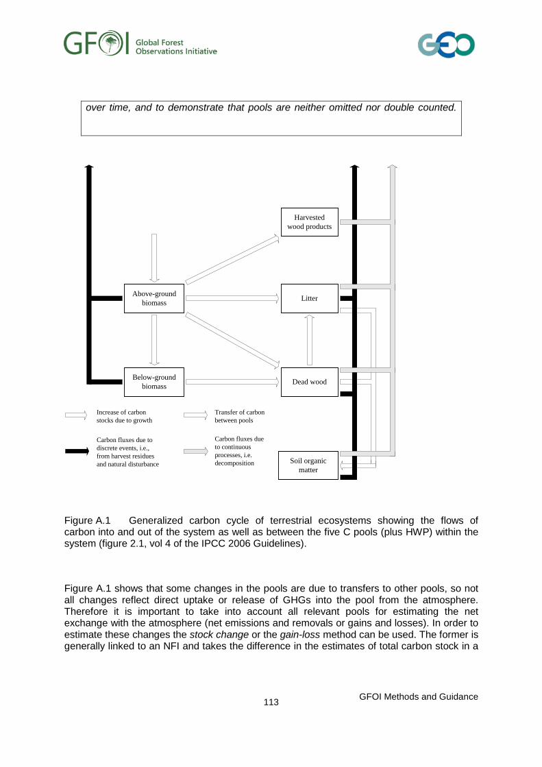
over time, and to demonstrate that pools are neither omitted nor double counted.
Figure A.1 Generalized carbon cycle of terrestrial ecosystems showing the flows of carbon into and out of the system as well as between the five C pools (plus HWP) within the system (figure 2.1, vol 4 of the IPCC 2006 Guidelines).
Figure A.1 shows that some changes in the pools are due to transfers to other pools, so not all changes reflect direct uptake or release of GHGs into the pool from the atmosphere. Therefore it is important to take into account all relevant pools for estimating the net exchange with the atmosphere (net emissions and removals or gains and losses). In order to estimate these changes the stock change or the gain-loss method can be used. The former is generally linked to an NFI and takes the difference in the estimates of total carbon stock in a
Litter
Dead wood
Above-groundbiomass
Below-groundbiomass
Soil organicmatter
Harvestedwood products
Increase of carbonstocks due to growth
Carbon fluxes due todiscrete events, i.e., from harvest residues and natural disturbance
Carbon fluxes dueto continuous processes, i.e.decomposition
Transfer of carbonbetween pools
GFOI Methods and Guidance
113

stratum at the beginning and end of a period. The latter subtracts the losses of carbon (e.g. harvest and disturbances) from the uptakes of carbon (e.g. growth).
The three tiers provided in the guidelines are distinguished by the level of detail and accuracy needed to convert forest changes to country level estimates of GHG fluxes. Consistent with the general characteristics set out in Box 1 of the main MGD text for both the GPG2003 and the 2006 Guidelines:
a) Tier 1 assumes that
• dead wood and litter pools can be lumped together as ‘dead organic matter’
• dead organic matter stocks are assumed to be steady for non-forest land use categories. For Forest Land converted to another land use, default values for estimating dead organic matter carbon stocks are provided.
b) Tier 2 generally uses the same equations as Tier 1 but requires country-specific information to replace the default parameters and also provides for a complete coverage of all the five pools.
c) Tier 3 typically uses complex modelling approaches calibrated to the ecosystems and national circumstances in question, often with remote sensing data to provide spatially explicit estimates.
Increased availability of remote sensing data makes Approach 3 (spatially explicit data) more accessible and it can in principle be used with any of the Tiers. How to use Approach 3 the focus of the MGD. Developing a national system based on Approach 3 and Tier 3, although potentially likely to be the most accurate, is the most data intense, and would make the highest demands on resources, infrastructure, data and national capability. Tier 2 and Approach 3, if sufficiently stratified, may in practice give comparable results. It may also be possible to use Tiers 2 and 3 in combination. The stepwise concept as envisaged in Decisions of the COP would allow countries to progress through the Tiers.
A1.6 Quality Assurance/Quality Control (QA/QC)
The overarching requirements are participation of an inventory compiler who is also responsible for coordinating QA/QC and verification activities, and definition of roles/responsibilities within the inventory. Section 5.5.2 of the GPG2003 introduces the idea of a QA/QC plan, which is described in more detail in section 6.5 of volume 1 of the 2006 GL and covers:
• Timeliness
• Completeness
• Consistency (internal consistency as well as time series consistency)
• Comparability
• Accuracy
• Transparency
• Improvement
GFOI Methods and Guidance
114

• General QC procedures that apply to all inventory categories (see Table 4);
• Category-specific QC procedures
• QA and review procedures
• QA/QC system interaction with uncertainty analyses
• Verification activities
• Reporting, documentation, and archiving procedures.
A QA/QC and verification system typically consists of the elements identified above. General QC procedures should be applied routinely to all categories and to the inventory compilation as a whole. Section 5.5 of GPG2003 discusses QA/QC and the corresponding parts of the 2006 GL are vol 1, chapter 6 (which discusses QA/QC in general, and vol 4, chapter 4 which provides additional material on QA/QC issues relating to forests).
The inventory agency should, where possible, check estimates of all managed land areas against independent sources. If the FAO database is the main source, the data should be cross-checked with other sources. The reasons for any differences in area estimates should be considered, action taken if necessary, and the results documented for the purposes of review. Areas used for activity data totals should be summed across all land-use categories to ensure that total area involved in the inventory and its stratification across climate and soil types remains constant over time. This helps ensure that areas are neither ‘created’ nor ‘lost’ over time, which could result in significant errors.
Table A.1.2: General Inventory Quality Control Procedures
QC Activity Procedures
Check that assumptions and criteria for the selection of activity data, emission factors, and other estimation parameters are documented.
Cross-check descriptions of activity data, emission factors and other estimation parameters with information on categories and ensure that these are properly recorded and archived.
Check for transcription errors in data input and references.
Confirm that bibliographical data references are properly cited in the internal documentation.
Cross-check a sample of input data from each category (either measurements or parameters used in calculations) for transcription errors.
GFOI Methods and Guidance
115

QC Activity Procedures
Check that emissions and removals are calculated correctly.
Reproduce a set of emissions and removals calculations.
Use a simple approximation method that gives similar results to the original and more complex calculation to ensure that there is no data input error or calculation error.
Check that parameters and units are correctly recorded and that appropriate conversion factors are used.
Check that units are properly labelled in calculation sheets.
Check that units are correctly carried through from beginning to end of calculations.
Check that conversion factors are correct.
Check that temporal and spatial adjustment factors are used correctly.
Check the integrity of database files.
Examine the included intrinsic documentation to:
• confirm that the appropriate data processing steps are correctly represented in the database.
• confirm that data relationships are correctly represented in the database.
• ensure that data fields are properly labelled and have the correct design specifications.
• ensure that adequate documentation of database, model structure and operation are archived.
Check for consistency in data between categories.
Identify parameters (e.g., activity data, constants) that are common to multiple categories and confirm that there is consistency in the values used for these parameters in the emission/removal calculations.
Check that the movement of inventory data among processing steps is correct.
Check that emissions and removals data are correctly aggregated from lower reporting levels to higher reporting levels when preparing summaries.
Check that emissions and removals data are correctly transcribed between different intermediate products.
GFOI Methods and Guidance
116
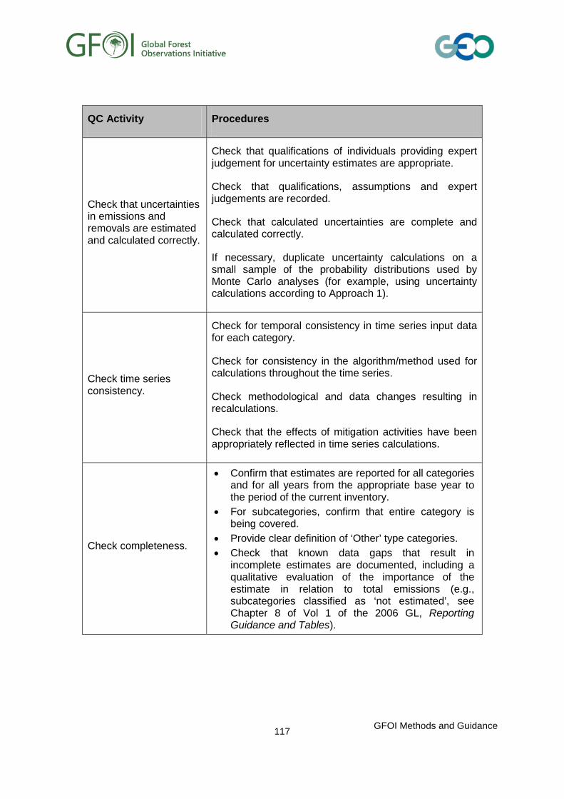
QC Activity Procedures
Check that uncertainties in emissions and removals are estimated and calculated correctly.
Check that qualifications of individuals providing expert judgement for uncertainty estimates are appropriate.
Check that qualifications, assumptions and expert judgements are recorded.
Check that calculated uncertainties are complete and calculated correctly.
If necessary, duplicate uncertainty calculations on a small sample of the probability distributions used by Monte Carlo analyses (for example, using uncertainty calculations according to Approach 1).
Check time series consistency.
Check for temporal consistency in time series input data for each category.
Check for consistency in the algorithm/method used for calculations throughout the time series.
Check methodological and data changes resulting in recalculations.
Check that the effects of mitigation activities have been appropriately reflected in time series calculations.
Check completeness.
• Confirm that estimates are reported for all categories and for all years from the appropriate base year to the period of the current inventory.
• For subcategories, confirm that entire category is being covered.
• Provide clear definition of ‘Other’ type categories. • Check that known data gaps that result in
incomplete estimates are documented, including a qualitative evaluation of the importance of the estimate in relation to total emissions (e.g., subcategories classified as ‘not estimated’, see Chapter 8 of Vol 1 of the 2006 GL, Reporting Guidance and Tables).
GFOI Methods and Guidance
117
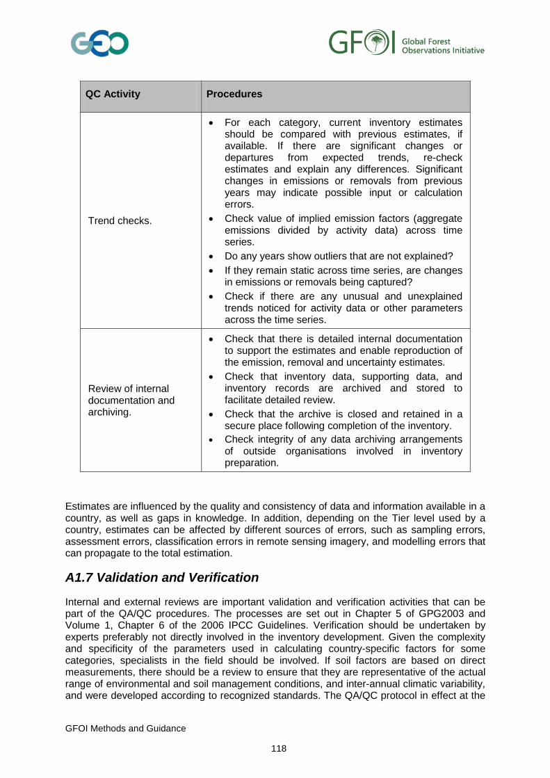
QC Activity Procedures
Trend checks.
• For each category, current inventory estimates should be compared with previous estimates, if available. If there are significant changes or departures from expected trends, re-check estimates and explain any differences. Significant changes in emissions or removals from previous years may indicate possible input or calculation errors.
• Check value of implied emission factors (aggregate emissions divided by activity data) across time series.
• Do any years show outliers that are not explained?
• If they remain static across time series, are changes in emissions or removals being captured?
• Check if there are any unusual and unexplained trends noticed for activity data or other parameters across the time series.
Review of internal documentation and archiving.
• Check that there is detailed internal documentation to support the estimates and enable reproduction of the emission, removal and uncertainty estimates.
• Check that inventory data, supporting data, and inventory records are archived and stored to facilitate detailed review.
• Check that the archive is closed and retained in a secure place following completion of the inventory.
• Check integrity of any data archiving arrangements of outside organisations involved in inventory preparation.
Estimates are influenced by the quality and consistency of data and information available in a country, as well as gaps in knowledge. In addition, depending on the Tier level used by a country, estimates can be affected by different sources of errors, such as sampling errors, assessment errors, classification errors in remote sensing imagery, and modelling errors that can propagate to the total estimation.
A1.7 Validation and Verification
Internal and external reviews are important validation and verification activities that can be part of the QA/QC procedures. The processes are set out in Chapter 5 of GPG2003 and Volume 1, Chapter 6 of the 2006 IPCC Guidelines. Verification should be undertaken by experts preferably not directly involved in the inventory development. Given the complexity and specificity of the parameters used in calculating country-specific factors for some categories, specialists in the field should be involved. If soil factors are based on direct measurements, there should be a review to ensure that they are representative of the actual range of environmental and soil management conditions, and inter-annual climatic variability, and were developed according to recognized standards. The QA/QC protocol in effect at the
GFOI Methods and Guidance
118

sites should also be reviewed and the resulting estimates compared between sites and with default-based estimates.
Comparison of different estimates, either independent estimates or those made using higher and lower tiers can provide additional means for verification. This can be applied to the emission and removal estimates or to input or intermediate data, especially area data.
It is currently difficult to verify emission and removal estimates independently. In principle, measurements of atmospheric concentrations can give completely independent estimates through approaches such as inverse modelling at continental, national or regional scales or by the use of proxy emissions 116 . Development of satellite measurements of the concentration of GHGs is underway but at present is too uncertain to provide accurate verification of national emissions.
116 Proxy emissions are made from measurements of a pollutant with a known emission rate and known emissions ratio to that whose emissions are being estimating. Then atmospheric measurements can be used to infer the emission rate of the unknown pollutant. See Use of Proxy Emission Databases 2006 GL Volume 1, page 6.22.
GFOI Methods and Guidance
119

Annex B Remote sensing data anticipated to be available through GFOI arrangement with the CEOS Space Data Coordination Group
Tables B1.1 and B1.2 provide an overview of the core optical and radar data anticipated to be available at the time of writing (CEOS Space Data Coordination Group, 2013). Table B1.3 provides details for additional optical and SAR satellite missions of potential interest but which are not currently considered core data sources either because they are in planning stage or are currently not available gratis.
These tables can be used to help select suitable data sets that may useful in obtaining activity data. Many of the satellites included in these tables do not have a global data acquisition strategy, so it is necessary to confirm that data are available for the region of interest. Information on satellite capabilities can be obtained via the CEOS MIM, which is an on-line database of instruments and measurements. Relevant links are the CEOS database handbook; http://database.eohandbook.com/. Information on sensor coverage can be obtained from the CEOS Visualisation Environment (COVE) tool at (http://www.ceos-cove.org/index.php/covetool/).
Table B1.1: Anticipated Core Optical Missions
Agency Mission Launch Resolution Swath Revisit Planned Duration
USGS/NASA
Landsat-7 1999 15m, 30m 185 km 16 days 5 years
USGS/NASA
Landsat-8 2013 15m, 30m 185 km 16 days 5 years
INPE/ CRESDA
CBERS-4 2015 5m 10m, 20m, 40m, 64m
60-866 km
26 days 3 years
ESA Sentinel 2A
2014 10m, 20m, 60m
290 km 10 days 7 years
ESA Sentinel 2B
2015 10m, 20m, 60m
290 km 10 days 7 years
GFOI Methods and Guidance
120

Table B1.2: Anticipated Core SAR Missions
Agency Mission Launch Band (wave length)
Polarization Resolution Revisit Duration
ESA Sentinel-1A and 1B
2014 and 2015
C (5.6 cm)
Single-, Dual-polarisation
9 m, 20 m, 50 m
12 days 7 years
CSA RADARSAT Constellation Mission (3 satellites)
2018 C (5.6 cm)
Single-, Dual-, Full- polarisation
1 m, 3 m, 5 m, 16 m, 50 m, 100 m
12 days 7 years
CONAE/ ASI
SAOCOM-1A and 1B
2015 and 2016
L (23.5 cm)
Single-, Dual-, Full- polarisation
10 m, 30 m, 50 m, 100 m
16 days 5 years
For additional information see CEOS MIM site at http://database.eohandbook.com.
GFOI Methods and Guidance
121
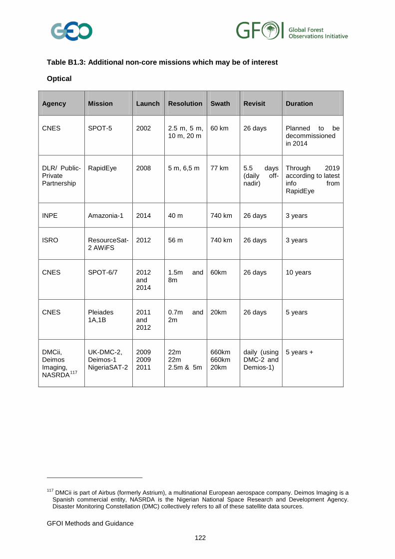
Table B1.3: Additional non-core missions which may be of interest
Optical
Agency Mission Launch Resolution Swath Revisit Duration
CNES SPOT-5 2002 2.5 m, 5 m, 10 m, 20 m
60 km 26 days Planned to be decommissioned in 2014
DLR/ Public-Private Partnership
RapidEye 2008 5 m, 6,5 m 77 km 5.5 days (daily off-nadir)
Through 2019 according to latest info from RapidEye
INPE Amazonia-1 2014 40 m 740 km 26 days 3 years
ISRO ResourceSat-2 AWiFS
2012 56 m 740 km 26 days 3 years
CNES SPOT-6/7 2012 and 2014
1.5m and 8m
60km 26 days 10 years
CNES Pleiades 1A,1B
2011 and 2012
0.7m and 2m
20km 26 days 5 years
DMCii, Deimos Imaging, NASRDA117
UK-DMC-2, Deimos-1 NigeriaSAT-2
2009 2009 2011
22m 22m 2.5m & 5m
660km 660km 20km
daily (using DMC-2 and Demios-1)
5 years +
117 DMCii is part of Airbus (formerly Astrium), a multinational European aerospace company. Deimos Imaging is a Spanish commercial entity, NASRDA is the Nigerian National Space Research and Development Agency. Disaster Monitoring Constellation (DMC) collectively refers to all of these satellite data sources.
GFOI Methods and Guidance
122

SAR
Agency Mission Launch
Band (wave
length)
Polarization Resolution
Revisit Duration
CSA RADARSAT-2
2007 C (5.6 cm)
Single-, Dual- , Full- polarisation
3 m, 5 m, 8 m, 10 m, 25m
24 days 7 years
DLR TerraSAR-X (TanDEM-X)
2007 and 2010
X (3.1 cm)
Single- and Dual- polarisation
1 m, 3 m, 16 m
11 days 8 years
ASI COSMO-SkyMed (4 satellites)
2007x2,2008 and 2010
X (3.1 cm)
Single-, Dual- , Full- polarisation
1 -100 m 16 days
JAXA ALOS PALSAR
2006 (end 2011)
L (23.6 cm)
Single-, Dual- , Full- polarisation
10 m, 20 m, 100 m
46 days 5 years
No longer operational
JAXA ALOS-2 2014 L (23.8 cm)
Single-, Dual- , Full- polarisation
3 m, 6 m, 10 m, 60 m, 100 m
14 days 5-7 years
UKSA NovaSAR-S 2015 (TBC)
S (9.4 cm)
Single-, Dual-, Triple-, Full polarisation (non-coherent)
6-30 m 14 days 7 years
ESA BIOMASS 2020 (TBC)
P (69.0 cm)
Full-polarisation
50 m Varying 5 years
Reference: CEOS Space Data Coordination Group, 2013. Baseline Global Acquisition Strategy for the Global Forest Observations Initiative (GFOI), 59 pp.
GFOI Methods and Guidance
123

Annex C Tier 3 Methods
This Annex describes in greater detail the possible Tier 3 implementations of the gain-loss method identified in Section 2.1.
C1.1 Representative Models
Instead of using emissions/removals factors, the representative model approach uses regional or species-specific management data and growth curves derived from research sites or from forest inventory data. These models can better represent changes in carbon stock due to activities not covered by emissions/removals factors (such as partial harvests or fire). This may allow the tracking of the fate of material (for example wood products), and can be readily expanded to other pools such as debris and soil carbon.
Applying representative models is similar to use of emissions/removals factors. The models are developed and the area they apply to identified through stratification. The models then run and the sum of the changes in carbon stocks each year for all the models equals the national estimate.
C1.2 Integrated Systems
Fully integrated systems aim to represent specific areas of land and estimate emissions using knowledge of site-specific conditions and management. These systems are typically more complex than the emissions/removals factor or the representative model methods, but have significant advantages including the greater ability to analyse the effects of management on emissions and to conduct detailed scenario analysis. Some represent combined forest and agricultural systems to allow better representation of emissions from land use and land-use change.
Fully integrated systems are Tier 3 and typically utilise mass-balance models that deal with all carbon pools and movements between them (Box C1). Currently operational systems use a variety of models from fully empirical modelling to hybrids between process and empirical models. There are currently no operational examples of full process-based approaches due to the amount of data required to calibrate and operate such models and the often unconstrained nature of their outputs.
There are two specific methods currently used in integrated systems: stand-based and pixel based models. The choice depends on availability of existing data (for example, remote sensing, mapping or national forest inventories), required outputs and cost.
GFOI Methods and Guidance
124

Box C1: Mass Balance Approaches
In mass-balance approaches (also known as ‘book-keeping’ or ‘conservation of mass’ approaches) the stocks and stock changes in each pool are based on transfers between pools using knowledge of the carbon cycle (Figure A.1 Carbon Cycle diagram). Mass-balance systems are well suited to estimating annual emissions/removals and tracking emissions/removals due to specific events such as harvesting or fire.
To be applied in national inventory systems, fully integrated, mass balance approaches need at least to:
• be able ability to represent accurately key flows of carbon, for example flows from natural processes (growth and decay), harvesting, fire, pest attack
• be parameterised using available or readily collectable data
• have checks and balances to prevent unrealistic results
• have tests to ensure that mass-balance is guaranteed at all steps through the model
• have inputs and outputs (flows) that match the carbon stock change.
C1.2.1 Stand based models
Stand based models are similar to the methods applied by forestry agencies to assess timber growing stock. In this configuration, the models are run on information for individually mapped stands corresponding to forest strata. The information includes growth rates, debris decay and soil carbon model parameters. The model is then run for each stand and the results summed for the entire forest area.
Stand based models are well suited to countries with detailed existing mapping of forestry activities such as harvest and replanting records. This mapping is not traditionally derived from remote sensing, but remote sensing can be used.
C1.2.2 Pixel based models
Pixel based models track individual pixels as land units, rather than stands. Pixel-based models aim to utilise the full strength of the remote sensing data through time and are suited to situations of multiple changes in land use or cover through time (for example, shifting agriculture). They are also well suited for deforestation and where there is little or no recorded history for forestry activities that could be applied in stand based models.
Pixel-based models estimate emissions and removal by modelling each and every pixel based on its land use history as derived from remote sensing. These models utilise both spatial and non-spatial data to parameterise the model for each pixel. This is achieved by integrating the remote sensing information with other spatial datasets (such as climate, productivity, soil type, forest type) and spatially referenced databases that provide species specific and management information. Summing the results of all the pixels creates the national estimate.
GFOI Methods and Guidance
125

C1.3 Operational Examples
C1.3.1 Stand based methods (Canada)
Summary
Canada applies a Tier 3 methodology to estimate emissions and removals from its Forest Land. Canada’s National Forest Carbon Monitoring, Accounting and Reporting System (NFCMARS - Kurz and Apps 2006) includes the CBM-CFS3118 model (Kull et al. 2006, Kurz et al. 2009, Stinson et al. 2011). This model integrates forest inventory and yield curves with spatially-referenced activity data on Forest Management and natural disturbances (fires, insect infestations) to estimate forest carbon stocks, carbon stock changes, CO2 emissions and removals and CH4 and N2O emissions.
The CBM-CFS3 model uses regional ecological and climate parameters to simulate carbon transfers among pools, to the forest products sector and to the atmosphere. The CBM-CFS3 model tracks emissions and removals as they actually occur over time. Harvesting and natural disturbance result in significant transfers of dead biomass carbon to the litter and dead organic matter pools. The model simulates the subsequent slow decay of the biomass that results in emissions for years or decades following the harvesting or natural disturbance, depending on the decay rates, as well as the removals that occur as forest stands regenerate after the disturbance.
As a result of this approach, which aims to estimate actual emissions and removals when they occur, the model is able to estimate more accurately the long-term impact of disturbances and provide accurate projections, as is required in the construction of a projected reference level. For further detail, see Chapter 7 and Annex 3.4 of Canada’s 2010 and 2011 National Inventory Reports119.
Area under forest management
Canada’s area under forest management (229 million hectares) covers about 66% of the country’s forests. The area subject to forest management is defined using an area-based approach as outlined by the IPCC (IPCC 2003) and includes:
i. lands managed for the sustainable harvest of wood fibre
ii. lands under intensive protection from natural disturbances (e.g., fire suppression to protect forest resources)
iii. protected areas, such as national and provincial parks that are managed to conserve forest ecological values.
Land Classification Databases
Canada’s monitoring system draws on the close collaboration among scientists and experts in different disciplines. It was recognized early on that the approaches, methods, tools and data that are available and most suitable for monitoring human activities in one land category
118 Carbon Budget Model for the Canadian Forest Sector 119 Can be downloaded from
http://unfccc.int/national_reports/annex_i_ghg_inventories/national_inventories_submissions/items/5888.php
GFOI Methods and Guidance
126

are not always appropriate for another. Important differences exist in the spatial framework specific to each land category, with the risk that activity data and estimates become spatially inconsistent.
In managed forests, the analysis units considered in the development of the inventory are the management units found in provincial and territorial forest inventories. For the purpose of this assessment, managed forests were classified into some 523 analysis units across 12 provinces and territories. Analysis units typically result from the intersection of administrative areas used for timber management and ecological boundaries.
The most suitable spatial framework for GHG estimation on agricultural lands (Cropland category) is the National Soil Database of the Canadian Soil Information System and its underlying soil landscapes. A full array of attributes are used to describe a distinct type of soil and its associated landscapes, such as surface form, slope, typical soil carbon content under native and dominant agricultural land use, and water table depth.
Forest characteristics
Age-class
The age-class distribution of the managed forest is captured by the forest inventory data and annual change information (due to harvesting, fire and insect infestations) used in the CBM-CFS3. The managed forest is composed of relatively old stands, with over half being 80 years or older in 2009. This age-class structure reflects past natural disturbances and management.
Increments
The input data for the CBM-CFS3 include information about forest growth rates for different forest types, site classes and regions. A description of how growth data by species and region are represented in the model and the source of the information can be found in Canada’s 2010 and 2011 National Inventory Reports (Chapter 7 and Annex 3.4), Kurz et al. (2009), and Stinson et al. (2011). The same growth and yield curves are used for both projected removals and for estimates of actual removals.
Rotation length
Canada’s managed forest is composed of substantial areas of slow-growing and relatively old stands. Harvesting decisions are determined according to provincial and territorial policies and regulations, taking into account the age of the forest, proximity to processing facilities, environmental considerations and other factors. Based on provincial and territorial input, CBM-CFS3 simulates harvesting at the appropriate age which varies by species and region and can include salvage logging of stands previously disturbed by fire or insects.
Business as usual forest management activities
The following projected management activities are considered: clear-cut harvesting, selection harvesting, salvage harvesting, shelter wood harvesting, commercial thinning and slash burning. The proportion of the total harvest accounted for by the various harvesting methods
GFOI Methods and Guidance
127

is projected using the recent average proportion of harvest to total harvest. The impacts of other silvicultural activities, such as tree planting, fertilization, and pre-commercial thinning are not accounted for explicitly because these activities are rarely implemented (fertilization, pre-commercial thinning) or their impacts are implicitly accounted for in the growth and yield data used in CBM-CFS3.
Harvested wood Products
Canada reports the HWP pool using three categories of (sawnwood; wood panels, paper) and a Tier 2 approach utilising data from the FAO, and country-specific density factors. This information is converted to carbon using Tier 2 estimates of emissions from both exported and domestically produced and consumed HWP.
Disturbances in the context of force majeure
Canada’s forest is continental in scale: a forest of this size means that almost every year some portion of the forest is affected by severe natural disturbances (i.e. wildfire and insect infestations). Canada predicts with a high degree of confidence the minimum level of wildfire that will occur every year. The background value of 95,000 hectares of managed forest burned each year is based on data from the past 51 years (1959-2009) which show that at least this amount burned during 90 percent of the years. The effects of background endemic insect infestations are captured in forest inventory and increment data.
Emissions from fire
Emissions from the background level of wildfire are calculated using a direct wildfire emissions factor of 0.132 kt CO2e per hectare burned. This factor is derived from data underlying Canada’s 2011 National Inventory Report, and is the average emissions factor for wildfires in the managed forest during 1990-2009. Non-CO2 emissions are substantial, amounting to 19 percent of the direct fire emissions.
References
Kurz WA, Apps MJ (2006) Developing Canada’s national forest carbon monitoring, accounting and reporting system to meet the reporting requirements of the Kyoto Protocol. Mitigation and Adaptation Strategies for Global Change,11, 33–43.
Kurz WA, Dymond CC, White TM, Stinson G, Shaw CH, Rampley GJ, Smyth C, Simpson BN, Neilson ET, Trofymow JA, Metsaranta J, Apps MJ. 2009. CBM-CFS3: A model of carbon-dynamics in forestry and land-use change implementing IPCC standards. Ecological Modelling 220:480–504.
Kull SJ, Kurz WA, Rampley GJ, Banfield GE, Schivatcheva RK, Apps MJ (2006) Operational-scale Carbon Budget Model of the Canadian Forest Sector (CBM-CFS3) Version 1.0: User’s Guide. Natural Resources Canada, Canadian Forest Service. Northern Forestry Centre, Edmonton.
Stinson, G., Kurz, W.A., Smyth, C.E., Neilson, E.T., Dymond, C.C., Metsaranta, J.M., Boisvenue, c., Rampley, G.J., White, Q.L., Blains, D. (2011) An inventory-based analysis of Canada’s managed forest carbon dynamics, 1990 to 2008. Global Change Biology 17: 2227-2244.
GFOI Methods and Guidance
128
C1.3.2 Pixel based methods (Australia)
The land area of Australia is about 760 million hectares. About 25% of total human induced greenhouse gas emissions in Australia result from activities such as agricultural production and land clearing. Given the size of Australia, it is not economically feasible or logistically practical to measure emissions and removals of greenhouse gases over such a large area with the use of direct emissions estimation methods alone e.g. field sampling. Given these national circumstances, the design of Australia’s national inventory system for the land sector relies heavily on the use of a modelling framework, to estimate the carbon stock change in biomass (above and belowground), litter and soil carbon resulting from land use and management activities.
In 1998 Australia embarked on a program to develop a comprehensive system to estimate emissions and removals from Australia’s land based sector 120 . The system integrates spatially referenced data with an empirically constrained, mass balance, carbon cycling ecosystem model (FullCAM) (Richards and Evans, 2000; Richards, 2001) to estimate carbon stock changes and greenhouse gas emissions (including all carbon pools, gases, lands and land use activities). FullCAM is an ecosystem model that calculates greenhouse gas emissions and removals in both forest and agricultural lands using a mass balance approach to carbon cycling. As a significant amount of emissions and removals of greenhouse gases occur during transitions between forest and agricultural land use, integration of agricultural and forestry modelling was considered essential. Currently the system supports Tier 3, Approach 3 spatial enumeration of emissions and removals calculations for the following sub-categories:
• Forest land converted to Cropland
• Forest land converted to Grassland
• Grassland converted to Forest land
• the agricultural system components of Cropland remaining cropland and Grassland remaining grassland.
Representation of Land
Australia uses a combination of geographically explicit data to represent land areas, consistent with Approach 2 and 3 as described in GPG2003. Data on areas of forest management for Forest Land remaining Forest Land are drawn from Australia’s National Forest Inventory. Supplementary spatial information from the Land Use Mapping programme of Australia’s Bureau of Agricultural Resource Economics and Sciences is used to identify land areas in the Cropland remaining Cropland, Grassland remaining Grassland, Wetlands, and Settlements categories.
120 For more detail see
http://www.climatechange.gov.au/sites/climatechange/files/documents/05_2013/AUS_NIR_2011_Vol2.pdf
GFOI Methods and Guidance
129

Forest Conversion Monitoring
Spatial enumeration is achieved through the use of a time series (since 1972) of Landsat satellite data which is used to determine change in forest extent. The forest cover change information is used with time series climate data and spatially referenced databases of land management practices. Australia monitors forest cover using national coverages of Landsat satellite data (MSS, TM, and ETM+) across 21 time epochs (periods between dates for which remote sensing data are available) from 1972 to 2012 which have been assembled and analysed for change. These national maps of forest cover are annual from 2004 and are used to detect fine scale changes in forest cover at a 25 m by 25 m resolution. Where forest cover change is identified in an epoch, the actual date of forest cover change in each 25 m by 25 m pixel is randomly allocated within the sequence of satellite pass dates.
Where change in forest area is detected, these changes are inspected by expert operators, to determine if these changes are due to human activity (e.g. harvesting, forest clearing, forest establishment) or due to natural events (e.g. fire, forest die-back, natural regrowth). The expert operators are trained in the use of standard criteria to distinguish human-induced from natural events and use databases of supporting information relating to land tenure and fire during this process.
FullCAM
FullCAM models both biological and management processes which affect carbon pools and transfers between pools in forest and agricultural systems. The exchanges of carbon, loss and uptake between the terrestrial biological system and the atmosphere are accounted for in the full, closed cycle mass balance model which includes all biomass, litter and soil pools. Analysis and reporting includes all carbon pools (biomass, dead organic matter and soil), greenhouse gases (CO2, CH4 and N2O), and covers both forest and non-forest land uses. It is an integrated suite of the following models:
• 3PG - the physiological growth model for forests (Landsberg and Wareing, 1997; Landsberg et al., 2000; Coops et al. 1998; Coops et al., 2000)
• CAMFor - the carbon accounting model for forests (Richards and Evans, 2000a),
• CAMAg - the carbon accounting model for cropping and grazing systems (Richards and Evans, 2000b)
• GENDEC - the microbial decomposition model GENDEC (Moorhead and Reynolds, 1991; Moorhead et al., 1999)
• Roth C - the Rothamsted Soil Carbon Model – Roth C (Jenkinson, et al., 1987, Jenkinson et al., 1991).
Developmental Lessons Learnt
To meet its objective of providing a comprehensive carbon accounting and projections capacity for land based activities, the National Inventory System (formerly known as the National Carbon Accounting System) has required strategic development of several key datasets and modelling and accounting tools. The system and underlying supporting data and science have been documented in many reports that are publicly available. Early reviews made it clear that approaches based on measurement were not feasible and that the calibration of relevant models would be required. The most significant value of FullCAM is that it allows for an ongoing evolution in the quality of any data inputs, be they for future
GFOI Methods and Guidance
130

accounting periods or improvements in fundamental input data or model calibration. Such ongoing improvements were not as readily made under the regional approaches envisaged formerly. FullCAM also provides for greater responsiveness to the various international reporting demands. The fine spatial resolution, activity-driven and time-based modelling provides a capacity to report at both project and continental scales, in response to specific activities, and with sensitivity to the timing of an activity.
References:
Coops, N.C., Wareing, R.H. and Landsberg, J.J., 1998: Assessing forest productivity in Australia and New Zealand using a physiologically-based model driven with averaged monthly weather data and satellite derived estimates of canopy photosynthetic capacity. Forest Ecology and Management 104:113-127.
Coops, N.C., Wareing, R.H. Brown, S. and Running, S.W.,2000: Predictions of Net Primary Production and seasonal patterns in water use with forest growth models using daily and monthly time-steps in south-eastern Oregon. Ecological Modelling (in press).
Jenkinson, D.S., Hart, P.B.S., Rayner, J.H. and Parry, L.C., 1987: Modelling the Turnover of Organic Matter in Long-Term Experiments at Rothamsted. INTERCOL Bulletin 15: 1– 8.
Jenkinson, D.S., Adams, D.E. and Wild, A., 1991: Model Estimates of CO2 Emissions from Soil in Response to Global Warming. Nature 351: 304–306.
Landsberg, J.J., Johnson, K.H., Albaugh, T.J., Allen, H.L. and McKeand, S.E., 2000: Applying 3-PG, a simple process-based model designed to produce practical results, to data from loblolly pine experiments. Forest Science .
Landsberg, J.J. and Wareing, R.H., 1997: A generalized model of forest productivity using simplified concepts of radiation-use efficiency, carbon balance, and partitioning. Forest Ecology and Management, 95: 209–228.
Moorhead, D.L., Currie, W.S., Rastetter, E.B., Parton, W.J. and Harmon, M.E., 1999: Climate and Litter Quality Controls on Decomposition: An Analysis of Modeling Approaches. Global Biogeochemical Cycles 13: 575–589.
Moorhead, D.L., and Reynolds, J.F., 1991: A General Model of Litter Decomposition in the Northern Chihuahuan Desert. Ecological Modelling 59: 197–219.
Richards, G.P. ed., 2001: Biomass Estimation: Approaches for Assessment of Stocks and Change. National Carbon Accounting System Technical Report No. 27. Australian Greenhouse Office, Canberra.
Richards, G.P. and Evans, D.W., 2000a: CAMFor User Manual v 3.35. National Carbon Accounting System Technical Report No. 26 (47pp), Australian Greenhouse Office, Canberra.
Richards, G.P. and Evans, D.W., 2000b: CAMAg National Carbon Accounting System, Australian Greenhouse Office, Canberra..
GFOI Methods and Guidance
131

Annex D Sampling
D1.1 Principles of sampling design
Any robust and reliable estimate of carbon in forest systems that is based on sampling must consider the following principles:
D1.1.1 Identifying individuals in the population that may be sampled
Individuals in a sampling system can range from plots to trees to point sampling. Whatever type is chosen, the individuals in the population being sampled must be clearly identifiable, and any exclusions and their treatment noted. When sampling to calibrate an allometric model for example, the logical unit is a tree, but care is needed to deal with different parts – e.g. for the roots what is the practical minimum diameter to be considered? Plots for measuring forest stand characteristics can vary in size with examples ranging from 0.02 ha to over 1 ha, and can also include clusters of sub-plots (related to each other through their spatial placements) or split designs (where size-based sub-populations are only measured on parts of a plot). Plot shape can be related to remotely sensed data attributes (e.g. pixel size of optical sensors) and are usually rectangular, square or circular. Optimum size and shape of plots will vary with forest conditions, with small area plots more typical in relatively homogeneous populations while larger plots are required in tropical forests where large trees result in high spatial variation in biomass (see 3.9.1.1).
D1.1.2 Selecting which individuals in the population to sample
Individuals are selected using either of two general approaches – design-based or model-based. Design-based (also called probability-based) approaches rely on the ability to assign a probability of selection to each individual in the population in order to make unbiased inferences about the population as a whole (mean or total size, and variance). For example, simple random sampling, the most basic of these designs, assigns an equal probability to each individual. More efficient design-based approaches may be employed when some structure in the population can be reliably identified. For example, stratified sampling uses strata of relatively homogenous sub-populations to improve inferences for a given sampling effort.
Model-based sampling selects individuals to allow the parameterisation of a model which is assumed to exist. Individuals therefore do not need to be selected using a probability-based system in order for inferences to be reliable and instead are usually selected to cover the range over which the model will be applied. Individuals may be selected to cover critical locations in the model domain, e.g. at the extremes, inflection points or where straight line relationships are anticipated. The way the individuals for measurement are identified and located should be transparent and free from personal bias.
D1.2 provides more details about the two approaches. They are not mutually exclusive, e.g. model-based approaches have been used within design-based approaches like stratified random sampling (Wood and Schreuder, 1986)
GFOI Methods and Guidance
132

D1.1.3 Selecting the number of individuals to sample
The number of individuals to sample is usually predetermined (sample size, n). Predetermined sample size approaches include those where:
• the number of samples is fixed by the available budget or need to have historical consistency
• a systematic approach is adopted to sample selection (e.g. by use of spatial grid of pre-determined resolution)
• a predetermined estimate has been made of the number required to produce usefully precise estimates.
Predetermined sample sizes to produce usefully precise estimates for the targeted population (or sub-population or stratum), or for parameter estimation in the case of model-based sampling, must be based on estimates of the variability of the (sub-) populations, which may be available from existing data (section 1.3.3) or reconnaissance surveys. Usefully precise estimates are often defined in terms of their desired sampling error, which in many cases is taken to be 10% as a default. The number of samples required under simple random sampling to achieve this level of sampling error is then:
n = CV% * t / √(10%) …A1
where CV% - Coefficient of Variation - is the sample standard deviation divided by the sample mean, expressed as a percentage, and t is taken from the t distribution with degrees of freedom equal to n minus the number of parameters being estimated, at the confidence desired, commonly 0.05 corresponding to 95% confidence.
Variability in design-based sampling refers to how much the individuals vary around their own mean, while the variability in model-based sampling refers to how much the models that may be parameterised from differing samples vary around the theoretically true model.
Sample sizes to detect rare occurrences (e.g. disturbance in forests such as deforestation) may need to be relatively large under simple random or stratified sampling designs. For example, a sample of size of n > 300 is required if annual levels of forest disturbance were expected to be only about 1% of the individuals, and individuals were selected via simple random sampling.
D1.1.4 Variable and supplementary sampling
Variable sample size approaches are rare in national scale inventories, but in some cases, the number of individuals sampled may be varied, with the measurements only stopping once sufficient evidence has been gathered so that a specific management decision can be made, or a set of predefined rules specifies an end condition. Examples include design-based approaches such as sequential sampling (e.g. continue selecting individuals at random until a decision is made that an insect infestation is sufficiently severe to warrant treatment), or adaptive cluster sampling (e.g. to estimate the number of trees that are rare but tend to occur
GFOI Methods and Guidance
133

in groups so if 1 is observed at a point there is an increased chance that there are more in the immediate area).
Supplementary sampling on the other hand may be required where an NFI or other extensive plot-based measurement system with a predefined sample size is already in place (Section 1.3.3), but does not adequately cover the whole population or results in a precision that is too poor to be reliable for the proposed forest monitoring system. Given the fundamental need for random selection (ability to determine the probability of individuals to be selected) in design-based sampling, the selection of additional samples will be difficult in some circumstances. Where a systematic approach to sampling was originally used (e.g. sample locations at the intersection of a regularly spaced grid that was randomly overlaid on the population), additional sampling points can be assigned as an extension of that grid into areas originally excluded. Such an extension is particularly relevant when individuals in the original sample had been excluded due to tenure (e.g. NFI did not extend to land managed by an Agricultural or Conservation Department even though it included forest by the national definition). The extended areas should maintain a separate identity if a stratified approach is used (Box 4), but the systematic grid may be manipulated (e.g. only select every 2 intersection) to ensure the sample size within the new stratum is appropriate (the number of samples per ha does not need to be constant between strata). Alternatively, if the stratum boundaries have not altered since the original sample but it has been determined that the precision of the stratum parameter estimates is insufficient, additional samples can be selected using the original sampling approach (e.g. truly random or, more commonly re-laying the same systematic grid but randomly choosing additional intersection points).
Where the original sample was not systematic and the population or strata boundaries have changed, it is very difficult to add samples under a design-based approach. In these cases a model-based approach may be more appropriate. The original sample data may be used to parameterise the hypothesized model, with additional samples chosen to improve the precision of the inferences about that model. For example, the original sample may be used to parameterise a model that relates LiDAR data or canopy characteristics to plot measurements of carbon. Additional plots should be established in strata not included in the original sample to ensure the hypothesised model is appropriate for the extended population. Under a model-based system, the additional samples need not use the original method of sample selection as inferences are not based on the selection design. Consequently if the inferences about the model are poor (e.g. confidence limits of the model around the strata mean is too wide) then additional, ad hoc, sample points can be added provided they use the same plot measurement protocols of the original sample. Under a model-based approach, additional samples that add the most information tend to be those measured at the extremes of the independent value range (e.g. tallest forests as determined by LiDAR) although sampling covering the full range of dependent variables, irrespective of how the underlying population is clumped along this range, is useful to ensure the model is appropriate.
D1.1.5 Using sample measurements to make inferences about the target population
The number of individuals selected for field measurement must be sufficient to make it likely that estimates of population means and sampling errors are unbiased (e.g. sufficient to allow the Central Limit Theorem to be applicable and to cover the variability within the target population).
Where total population parameters are calculated from the sum of sub-samples or separate models or relationships, double counting of pools must be avoided. All errors must, a far as possible, be identified, quantified and managed. These errors include sampling error, measurement error and modelled error.
GFOI Methods and Guidance
134

D1.2 Design and Model -Based Sampling
Design-based sampling, also known as probability-based sampling is a widely-known sampling system. In this system, sample locations are selected by a pre-determined random (probability based) process. The most frequent examples are simple random sampling, and stratified (or restricted) random sampling, but cluster, double and sequential sampling approaches are also common. Systematic sampling, provided the starting point is randomly located, falls into this group. The random process determines the probability of selection for every possible location, and every possible location must have a probability greater than zero. These probabilities are the sole basis for drawing conclusions or "inferences" - usually formulated as probability statements - from the sample about the population size (total, mean), proportion of the population with given characteristics (such as disturbance or occurrence of a rare species), or variance. This means that, if a sample is selected correctly according to the chosen random design, any inference based on these probabilities is valid and calculations do not rely on any assumption about the spatial distribution or other pattern in the population. Apart from measurement error, sampling is the only source of stochasticity considered and this error can be readily calculated. NFIs are typical design-based sampling systems with plots established on systemic grids (with or without stratification) where the probability of selection for each plot (within a stratum) is equal and known. Design-based samples can also include those where the probability of selection is random but not equal, say proportional to, size (as in point sampling or variable radius sampling) or to a prediction (estimated volume or height as in 3P sampling – Probability Proportional to Prediction).
Model-based sampling systems hypothesise the existence of a model that relates predictor (X or independent) variables to the response (Y, or dependent) variables of interest. A sample is drawn to allow inferences about this model, and the distribution of data around the mean model values. Two types of inference are therefore made under model-based sampling, concerning: (i) the values at locations unvisited during sampling; and (ii) parameters of the model, including the confidence intervals of the parameterised model. Estimates of the mean Y in a model-based system would be based on the inferences about the model at the value of the mean X. For example, a model-based system that uses LiDAR as a predictor variable might rely on an assumption that biomass is linearly related to the mean height above the ground of the returns per unit area. A purposive sample of field locations could be drawn to parameterise this model and the mean biomass of the forest could be estimated from this parameterised model and the mean LiDAR return over the entire forest. Accuracy of these estimates would depend on the legitimacy of the assumed model and the actual sample locations (within the model space). Inferences at specific locations could also be made although these will be less precise than the population mean estimates. Model-based systems do not assume that the probabilities of any sample location (pair of X and Y variables) are determined by the design, but rather they are an outcome of the chosen random model – for any given X, the Y values are likely to be centred around the model mean. Where the variation in Y around the model prediction is less than the total variation in Y, model-based systems can provide increased precision of estimates.
GFOI Methods and Guidance
135

Annex E Choice and use of emission and removal factors for each REDD+ activity
For the purposes of GHG estimation, the REDD+ activities discussed in Section 2.2 can be conveniently grouped into the following three categories:
• conversion of forests to non-Forest Land uses (deforestation). This requires the estimation of GHG emissions resulting directly from the deforestation event itself, as well as the emissions and removals resulting from the new land use (e.g. agriculture).
• conversion of non-Forest Land to forest which results in enhancement of forest carbon stocks (afforestation, or reforestation of land previously converted from forest to another land use). This requires estimation of the difference in GHG emissions and removals between the old and new land uses.
• changes in GHG emissions and removals in forests remaining forests. This covers: forest degradation, sustainable management of forests, enhancement of C stocks (within an existing forest), and conservation of C stocks. The GHG outcome can be either positive (e.g. protection of existing C stocks or increase in C stocks under changed management; reduction in emissions from decomposition of peat or from fire in degraded peat forests) or negative (e.g. progressive loss of biomass C under forest degradation, conversion of high biomass native forests to planted forest, or loss of soil C due to drainage of organic soils).
E1.1 Deforestation
Using the land classes defined by IPCC GPG2003, deforestation is estimated as the sum over transitions to other land uses from forest. IPCC estimates the associated emissions and removals as the sum of the consequences of transitions from forest to other land uses. It is advisable that after the basic classification exemplified here by primary forest, modified natural forest and planted forest, there is sub-stratification of the data by forest ecosystem undergoing conversion and by land use after conversion, including distinguishing between areas of organic and mineral soil. Alternatively countries may stratify first by ecosystem type. Countries may wish also to stratify according to drivers of deforestation since this may help develop understanding of causal relationships between drivers and deforestation rates. The stratification should enable identification of natural forest since this information may be required under the safeguards provisions agreed in Cancun.
E1.1.1 Emission/Removals Factors
1. Carbon pools
Emission and removal factors are needed for carbon in biomass, DOM and soils. For Tier 1 estimation, default values or assumptions can be found in the GPG2003 and the 2006GL. For Tier 2 estimation, these factors will need to be defined for all important combinations of forest type/new land use transition. Field studies will be required to estimate the biomass and DOM in representative forests before clearing, and the fate of these after deforestation. Forest biomass stocks in areas at risk of deforestation may be lower than in undisturbed forest of nominally the same ecosystem, because increased accessibility may have led to gradual degradation. Sampling in these areas along the lines set out in Section 2.2 and Annex D should be conducted. DOM stocks should be measured at the same time as other sampling is conducted.
GFOI Methods and Guidance
136

Biomass may be harvested and removed from the site, be left to decay on site, or be burnt – the relative amounts need to be known in order to account for the pattern of carbon loss, and to estimate non-CO2 emissions in fire. Depending on the new land use, there may be some removals of C into newly created biomass or DOM and field studies will be needed to estimate this.
Deforestation often leads to loss of soil C over several decades, with the amount of loss depending on soil type and the nature of the new land use. Extensive field studies are required to define the magnitude of change under Tier 2, or calibrated and tested models can be used to estimate change (Tier 3). Realistically, unless significant work has already been done, the new field studies will require many years of work and will be expensive to conduct. The only short-term option is to use existing default methodology for soil C change using values that are matched to the soils, land use transitions and climatic conditions where deforestation is taking place. Sources of default information are the GPG2003, the 2006GL, the IPCC emissions factors data base, and published scientific reviews. It is important that there be critical analysis of the applicability of selected defaults to the in-country conditions.
2. Non-CO2 GHG emissions
The effects of deforestation on non-CO2 GHG emissions mainly result from:
• burning of biomass and dead organic matter remaining on site
• on-going emissions from soils over time under the new land use, including any emissions resulting from the application of N fertilizers
• emissions resulting from enteric fermentation or manure management where the land is converted to agriculture.
Advice for estimating these emissions using IPCC approaches is given in Section 3.8.
E1.1.2 Supporting data
Stratification requires information on forest type and disturbance history so that appropriate emissions/removals factors, allometric models, etc, can be selected. Information is also required on the new land use because this markedly affects future emissions. Soil type will be needed to distinguish between mineral and organic (particularly peat) soils. Local and national soil maps should be used if available. International soil maps are very unlikely to be reliable at the spatial scale at which deforestation occurs.
E1.2 Afforestation and reforestation
Emissions/removals from afforestation and reforestation can be estimated using either the gain-loss method, or a combination of that method and the stock change method (for estimating change in biomass), if a country has an NFI with sampling strategy designed effectively to detect change in these activities (section 2.2).
GFOI Methods and Guidance
137

E1.2.1 Emission Factors
1. Carbon pools
Rates of biomass accumulation as a function of forest type and stand age can be taken at Tier 1 from IPCC advice on land converted to forest. For higher Tiers, country-specific data on rates of forest growth are needed for relevant species and locations (site growing conditions). Well-designed forest inventories or other sampling are the primary source of this data. Such data can also be used to derive growth models that can be used for spatial and temporal estimation of change in biomass carbon stocks, and are also needed to estimate loss of biomass caused by fire, disease or partial harvesting (e.g. thinning), and the effects of these on subsequent rates of growth. Once reliable growth models have been established, these can be combined with estimates of biomass loss (e.g. statistics on harvested wood) to enable the gain-loss approach to be used to estimate net change in biomass. Changes in DOM are generally small relative to change in biomass after afforestation/reforestation, but after harvest of planted forest significant amounts of residue may be created, and these need to be estimated using field sampling.
Loss of soil C from disturbance during the establishment of forested areas should be included, as should any longer-term changes (gains or losses) under the forest. Default (Tier 1) soil C change factors can be found in the IPCC GPG2003 and 2006GL. Development of emissions/removals factors for Tier 2 approaches will involve extensive field work or scientific review121.
2. Non-CO2 GHG emissions
Non-CO2 GHG emissions are likely to be small from such activities, but could result where fertilizer is added to the newly established forest or where fire (either wildfire or managed fire) occurs in the forest. Where forests are subsequently harvested (sometimes they are not when the plantings are established for environmental values), there will be non-CO2 emissions where fire is used to assist natural regeneration or preparation of the site for a new planting.
Advice on how to estimate these emissions is provided in Section 3.8.
E1.2.2 Supporting data
Data will be needed on the previous land use, the type of plantation established and the year of establishment, location (as a guide to soil types and potential growth rates) and the management regime (especially harvesting) applied.
E1.3 Forest Degradation
From a GHG inventory perspective, degradation means sustained reduction of forest carbon stocks (in either biomass, DOM or soil) without crossing deforestation thresholds, or a reduced capacity of forests to recover after disturbance. Methods for estimating change in GHG emissions are given in section 2.2.
121 ISRIC provide an international database for soil properties including SOC that can be relevant to support assessment of soil C. http://www.isric.org/
GFOI Methods and Guidance
138

E1.3.1 Emission Factors
1. Carbon pools
The effect on emissions can be estimated from the rates of expansion or contraction (in the case of rehabilitated forests) of degraded areas, whether the areas are estimated directly, or are estimated from indicators of degradation. Appropriate emissions/removals factors need be established that can be applied to these areas. Unless the emissions/removals factors are shown to be reliable, the estimated GHG emissions resulting from forest disturbances, or removals that occur during recovery from disturbance will be very uncertain.
For biomass stock change, emissions/removals factors will need to be established for important combinations of forest type and disturbance (harvest, fire, drainage, disease) type. Where available, forest inventories can be a useful source of information, but may need to be supplemented by additional targeted field sampling in specific locations (see section 2.2). Volumes of timber extracted (if known) can be useful in estimating potential loss of biomass stocks if these are compared with rates of regrowth of forest on the degrading areas. Rates of regrowth (removal factor) can be taken at Tier 1 from the IPCC Guidelines or from country specific data. The area to which regrowth is applied needs to be the area actually regrowing, not the total forest area, otherwise the estimate of carbon sequestered in regrowth will be greatly overestimated. For DOM, specific sampling programs are likely to be required to determine emissions/removals factors for important forest types/disturbances. For fire, carbon emissions are estimated from the amount of fuel combusted , and defaults to allow Tier 1 estimates for biomass and DOM are provided in IPCC 2006 GL. Countries are encouraged to derive their own emission factors for fire, but this will require extensive field and laboratory research, so that in the interim, Tier 1 defaults should be used.
For estimating change in soil C, use the approach outlined above for mineral soils. For disturbed organic soils, loss of soil carbon stocks can be very large and on-going especially following drainage or where fire combusts organic matter. Following drainage, the emission factors provided for Wetlands in IPCC (2013) can be used. Following re-wetting (rehabilitation of peat land) use the IPCC (2013) emission factors, or assume that soil CO2 emissions will be reduced to zero. Section 3.9.4 of the main text of the MGD provides advice on where to access emissions factors related to estimating emissions from peat fires.
2. Non-CO2 GHG emissions
Multiple factors can lead to forest degradation, some of which can affect emissions of non-CO2 GHGs e.g. combustion of biomass and dead organic matter by wildfire or too-frequent management burning, soil inundation due to practices which change local hydrology, and drainage of organic (peat) soils (which also renders them susceptible to fire).
Degradation is complex, with highly varying local consequences for non-CO2 GHG emissions and uptake, and is relatively poorly understood. Whilst generic guidance for estimating emissions for some of these is provided in GPG2003,2006 GL and the IPCC Wetlands Suppliment, there is a requirement for local activity data and corresponding emissions factors e.g. on the amount of fuel consumed by fire in forests degraded by partial logging, areas of forest subject to inundation, area of peat forest drained or burnt.
GFOI Methods and Guidance
139

There is a need for further research to strengthen the basis for default emission factors for tropical peat fires because it has a major impact on estimation of CO2 emissions (Peat & GHG Group, 2011).
E1.3.2 Supporting data
Stratification of the forest into important forest types with differing biomass density and rate of regrowth following disturbance is needed. Information on the nature and timing of forest disturbance (e.g. extent and intensity of fire, type and extent of drainage) is important in interpreting the temporal pattern of both emissions and removals of GHGs. Soil maps are important for estimating carbon stocks and their vulnerability to loss (especially the extent of peat soils). Estimates of wood harvested from specific areas will be useful in estimating change in biomass stocks in the forest.
E1.4 Restoration of degraded tropical peat lands.
Large areas of peat forests have been degraded globally by heavy logging or deforestation, drainage, or repeated wildfire. GHG emissions can be very high, especially in the tropics, from such disturbed forests and continue for many decades as peat continues to decompose or is irregularly burnt by wildfire. Rehabilitation can involve re-wetting (blocking of drainage systems), fire prevention and suppression, and re-vegetation. Rehabilitation assists in slowing, and the gradual reversing, of degradation processes that were leading to on-going emissions. Emissions can be estimated in the same way as for afforestation or reforestation with special attention given to soil emissions before and after the conversion. The IPCC Wetlands Supplement provides Chapter 3 provides Tier 1 guidance for assessing the greenhouse gas (CO2, CH4 and N2O) emissions and removals from rewetted organic soils by climate region and general guidance for utilizing higher tier methodologies.
Spatial data will be required on the type and area of forest degraded by harvesting, drainage or wildfire in the base year before rehabilitation starts. Data on temporal change are then needed in the area of forest burnt by wildfires and the amount of above-ground fuel and peat combusted, the area of forest effectively re-flooded or protected from wildfire, and the area of forest effectively re-established by natural regeneration or planting.
E1.4.1 Emission Factors
1. Carbon pools
Advice is provided above on estimating C change in degraded forests. For disturbed tropical peat land, refer to the IPCC Wetlands Supplement, Section 2.2.1 for lands remaining in a land use category and Section 2.3.1 for lands converted to a new land use category..
2. Non-CO2 GHG emissions
Advice for estimating non- CO2 emissions is given in the IPCC Wetlands Supplement for drained organic soils in Section 2.2.2 for land remaining in a land use category and Section 2.3.2 for lands converted to a new land use category.
E1.4.2 Supporting data
A map of forest disturbance history will help establish the reasons for the current degraded state of the forest, and the likely response to management interventions
GFOI Methods and Guidance
140

E1.5 Conservation, sustainable management of forests and enhancement (in existing forests) of forest carbon stocks
All pools and fluxes need to be estimated in order to quantify the overall effects of changed management practices. Emissions/removals can be estimated using either the gain-loss method, or a combination of that method and the stock change method (for estimating change in biomass). The stock change approach for biomass will only be possible if a country has an NFI with sampling strategy designed to effectively detect change in these activities, and the inventory is systematically updated. If this is not the case countries should use the gain-loss method (see section 2.2).
Regional and finer-scale management plans should indicate areas where the objective is sustainable forest management, or management of areas for conservation, or to enhance forest carbon stocks. These areas should be checked against records of the actual implementation of intended management practices. There is a need to have total coverage of the forest, so that both land managed by governments and by the private sector is included. Any areas subject to deforestation or forest degradation should not be included in areas subject to conservation, sustainable management of forests, or management to enhance forest carbon stocks.
E1.5.1 Emission Factors
1. Carbon pools
See sections above.
2. Non-CO2 GHG emissions
There is the potential to reduce non-CO2 GHG emissions via improved management practices, especially those emissions derived from drainage of peat forests, fire or fertilizer use.
E1.5.2 Supporting data
A forest type and land tenure map is required, as is access to regional and finer-scale forest management plans. A map of forest disturbance histories will be valuable in guiding current forest condition (e.g. age of regrowth) and thus potential for increases in biomass stocks under changed management. Where a country does not have an NFI, models to estimate forest growth rates under changed management will be required.
E1.6 Conversion of natural forests
Whilst this is not a REDD+ activity, countries may need to identify separately the conversion of natural forest under the safeguards provisions for REDD+.
Methods for estimating the emissions associated with the step of removing the natural forest are described under deforestation, and methods for estimating emissions/removals during the establishment and growth of new planted forest are described in section 2.2.
GFOI Methods and Guidance
141
In the early stages of conversion it may be difficult to distinguish this activity from deforestation since both will incur loss of crown cover. The establishment of planted forest may be difficult to detect remotely in the early years. Thus, ground based data from forestry authorities and the private sector on areas of land subject to this activity are likely to be needed. In the absence of this information removal of natural forest should initially be estimated as deforestation. Key activity data and corresponding emissions/removal factors required are the area and type of forest converted, the area of forest drained, the area of forest burnt during site preparation and the amount of fuel consumed per unit area, the type and growth rate of the new plantation established, and the amount of any N fertilizer applied to the planted forest.
E1.6.1 Emission Factors
1. Carbon pools
See above sections covering removal of the natural forest, and the establishment and growth of a new plantation.
2. Non-CO2 GHG emissions
Conversion of native forests to plantations can result in non-CO2 emissions during both the removal of the natural forest, and during the establishment and on-going management of the plantation. The method of site preparation has a significant effect on non-CO2 GHG emissions e.g. where drainage and /or fire are employed the emissions can be very high. There can also be on-going emissions where N fertilizer is added to increase growth of plantation trees.
E1.6.2 Supporting data
Data will be needed on the type of natural forest converted and the biomass stock (affected by prior disturbance) at the time of conversion, the type of plantation established and the year of establishment, and on location which will affect potential growth rates. A soil map that can be used to infer soil C stocks and likelihood of drainage of organic soils is also required.
GFOI Methods and Guidance
142
Annex F Brief Review of the Potential for Direct Estimation of Biomass by Remote Sensing
There is active research on methods to estimate biomass in tropical forests using remote sensing techniques, including by analysis of spectral indices and use of radar and LiDAR. In general these methods require calibration using ground-based data. Saturation may be a problem, especially in tropical countries because the correlation between biomass and the remote sensing data may not be effective at high biomass densities.
A key issue when using tree height (estimated using LiDAR or RADAR) to estimate biomass, is that the relationship between height and biomass is likely to differ markedly with forest type, tree age, speciation, and following forest disturbance (e.g. between primary and secondary forest). Such differences need to be understood and taken into account in order to improve estimates of forest biomass and change in biomass as part of MRV.
This review leads to the conclusion that existing large-scale biomass maps derived from remote sensing data should not be used without extensive in-country testing to confirm that they are reliable for application in specific forest types and at varying spatial scales. Biomass estimation error using remote sensing is high at the plot scale (< 1 ha) and up to 1 sq km (100 ha) (Saatchi et al., 2011) and therefore robust field estimates of biomass based on adequate plot size, sufficient spatial sampling, and use of appropriate allometrics are needed to enable such testing (e.g. Chave, et.al., 2004; Avitabile et al., 2011). This means that currently the method is unlikely to be cost efficient.
A brief review of recent work to produce biomass estimates for tropical forests follows.
F1.1 Use of LIDAR for biomass estimation
Biomass estimates are usually obtained by combining LiDAR data with field observations and sometimes optical data e.g. the use of MODIS surface reflectance for obtaining wall-to-wall maps of biomass from point-based estimates as in Baccini et al. (2011).
Baccini et al. (2008) produced a spatial biomass map of Africa by combining remote sensing and field estimates of biomass derived from a range of sources. Mitchard et.al. (2011) criticised this map, claiming that the ground data used for calibrating the remote sensing were inadequate, and resulted in significant underestimation of field estimates of biomass, especially for areas with high biomass densities. Avitabile et.al. (2011) reported poor correspondence between 7 biomass maps (derived either by extrapolation of field estimates of biomass, or derived using remote sensing) for Uganda, both in terms of average biomass densities and spatial patterns. They concluded that the next critical step to increasing reliability of biomass maps was the collection of more reliable field biomass data for key forest types.
Saatchi et.al. (2011) used remote sensing to derive a biomass map for tropical forests at 1 km resolution, and to estimate the errors of biomass estimates made at differing spatial scales. They established a relationship between forest stand height and biomass at 493 locations across the tropics. This relationship was able to predict ground estimates of biomass for many other locations with an uncertainty of about 24% on average. Estimates of
GFOI Methods and Guidance
143

forest height derived from space-borne LiDAR were then used to estimate biomass at many more locations. The biomass estimates derived from ground measurements and those estimated using LiDAR were then extrapolated across the entire tropical forest using a data-fusion model and satellite imagery from a range of sources. No validation of these new biomass estimates appears to have been undertaken. The authors assumed that their initial field estimates of biomass were error-free, but acknowledged that there may have been significant and systematic non-random errors in the estimates used. Analysis by Chave, et.al. (2004) of the sources of error involved in biomass estimation at both plot and landscape scale in tropical forests, suggests that such errors were very likely. Chave, et. al 2004 provide advice on how to minimize biomass estimation errors, and identified the critical importance of appropriate selection of allometric models which they concluded were a high contributor to uncertainty.
Baccini et.al. (2012) used remote sensing to generate a biomass map for tropical forests at 500m resolution. They used generalized (pan tropical) allometric models to convert forest inventory data to forest biomass at a range of locations across several countries, and then correlated biomass with tree height estimated using space-borne LiDAR. Using generalized allometrics to estimate biomass can result in errors in estimates at particular locations (e.g. Basuki et al., 2010), and the extent of bias in model calibration in the Baccini et al. (2012) study is unknown. Again, no independent validation was conducted, but comparisons with several country-level estimates of biomass stocks estimated by Saatchi et al. (2011) showed differences of up to 50%.
F1.2 Sources of LIDAR
The most feasible approach for obtaining biomass estimates from remote sensing data is to make use of LiDAR-based measurements of vegetation structure. LiDAR systems emit laser pulses and by measuring the timing and intensity of the returns, three-dimensional information on vegetation structure is inferred which in turn allows for prediction of forest structure attributes related to aboveground biomass. There are two main sources of LiDAR data: (1) small footprint, airborne LiDAR data and (2) full waveform, space-borne LiDAR data. At the time of writing there is no operational LiDAR satellite; data availability is limited to what is available from the GLAS instrument on the now defunct ICESat satellite between 2003 and 2009.
F1.2.1 Airborne LiDAR data
Airborne LiDAR data, if available for a sample of the study area, can be used to estimate biomass. The LiDAR data provides three-dimensional information on the vegetation structure that can be regressed against plot-level aboveground measurements of biomass to provide biomass estimates for each LiDAR observation. Even if allometric models exist for a range of conditions which allow for biomass estimation without in situ collection of biomass, biomass measurements within the area covered by the LiDAR flight tracks can help ensure that regional and local variation in the LiDAR-biomass relationship is included (Asner, 2009). Examples of how to use airborne LiDAR data together with field plots to estimate biomass are provided by: Asner et al. (2010) (IPCC-compliant estimates of carbon stocks and emissions in the Peruvian Amazon); Nelson et al. (2004) (biomass estimation in Delaware, United States); Næsset et al (2013) (biomass change estimates in boreal forests, Norway); and Lefsky et al. (1999) (biomass estimation in deciduous forests in Maryland, United States).
GFOI Methods and Guidance
144

F1.2.2 Satellite LiDAR data
LiDAR observations from space are currently limited to data from the GLAS sensor on board the ICESat. The sensor collected LiDAR data from 2003 to 2009 which is available for free download at NASA Reverb: http://reverb.echo.nasa.gov. ICESat-2, which will carry LiDAR instruments, is planned for launch in early 2016. No other missions are planned at the time of writing. Therefore there is a data gap in space borne LiDAR observations between 2009 and 2015.
Research indicates that, while it is possible to estimate tree height from ICESat/GLAS data which in turn can be regressed to obtain biomass estimates (Sun et al., 2007), estimating tree height from GLAS data is less straightforward compared with using airborne, small footprint LiDAR data. On sloping areas, topographic information is required to estimate tree height because of the elliptical shape of the GLAS footprint (Lefksy et al., 2005). Sources that provide descriptions of using GLAS data for estimating tree height and biomass include: Baccini et al (2012); Saatchi et al (2011); Nelson et al (2008); Boudreau et al. (2008); Lefksy et al. (2005).
Existing large-scale biomass products include:
• The National Level Carbon Stock Dataset (Tropics) Woods Hole Research Center (WHRC) provides maps of above-ground live woody biomass for the tropics. Using a combination of field measurements and space-borne LiDAR observations at 70 m spatial resolution from the Geoscience Laser Altimeter System (GLAS) instrument on board the Ice, Cloud and land Elevation Satellite (ICESat), and optical MODIS imagery at 500 m spatial resolution, the WHRC National Level Carbon Stock Dataset provides above-ground live woody biomass at 500 m resolution for the tropics 2007-2008 (Baccini et al., 2012). The data are provided via a website at: http://www.whrc.org/mapping/pantropical/carbondataset_form.htm
• The National Biomass and Carbon Dataset (NBCD2000) WHRC provides a 30 m biomass product for the coterminous United States. This map does not cover tropical areas, but it provides a model for how NFI plot data can be combined with remote sensing data to make maps of biomass. NBCD2000 is based on a combination of data from the USDA Forest Service Forest Inventory and Analysis (FIA), the 2000 Shuttle Radar Topography Mission (SRTM) and Landsat-7/ ETM+. It provides basal area-weighted canopy height, above-ground live dry biomass, and standing carbon stock for the year 2000 (Kellndorfer, et al., 2012). Access can be obtained via: http://www.whrc.org/mapping/nbcd/nbcd_reg.html
• The JPL Carbon Maps. The Jet Propulsion Laboratory of NASA and the California Institute of Technology provide a biomass product similar to that of the WHRC National Level Carbon Stock Dataset. The maps provide forest above-ground carbon and biomass for sub-Saharan Africa, the Americas south of latitude 30° N, and South-East Asia and Australia between the latitudes of 40° N and 30° S at 1 km resolution. Point-based estimates of biomass generated from a combination of field data and space-borne LiDAR data from ICESat/GLAS were extrapolated using
GFOI Methods and Guidance
145

optical data from MODIS and radar data from SRTM and QuickSCAT (Saatchi et al., 2011). Access can be obtained via: http://carbon.jpl.nasa.gov/data/dataMain.cfm
F1.3 Use of Synthetic Aperture Radar (SAR) for biomass estimation
Although synthetic aperture radar (SAR) has demonstrated potential for estimating aboveground biomass, there are limitations arising from:
• rapid saturation of the signal at low aboveground biomass stock
• terrain
• rainfall and soil moisture effects
• localised algorithm development focussing on a single biome or mono-species stands
• lack of consistency in estimates as a function of sensor parameters.
Calibration of the retrieval algorithm depends on reliable ground data, which need to be collected under a representative range of environmental conditions. This means that there is limited transferability of algorithms within and between different forest structural types and, so far, no reliable means of estimating aboveground biomass (Lucas et al., 2010). SAR based estimation of above-ground biomass has been more successful in temperate than in tropical forests, due largely to fewer species and lower biomass (Castro et al., 2003). Increased sensitivity has been achieved using ratios or correlations between multi-frequency, multi-polarisation backscatter and biomass components (Castro et al., 2003). Alternative approaches, including SAR interferometry, polarimetric interferometry, tomography and integration with LiDAR and other data are the focus of current investigations.
SAR has demonstrated capacity to quantify biomass up to a certain level, depending on the frequency used. Once saturation of the signal is reached, the data are no longer useful for biomass estimation (Böttcher, et al. 7, 2009, Gibbs, et al. 2007). Cross-polarised backscatter demonstrates greater sensitivity to forest biomass than co-polarised backscatter. The use of multiple polarisations is recommended for use in retrieval algorithms (Castro et al., 2003). L-band SAR is useful for discriminating regrowth stage and estimating biomass in low biomass (40-150 t/ha) forests. Dual polarisation and dual-season coverage is required. C-band SAR is only useful in very low biomass forests (30-50 t/ha). The shorter wavelength does not penetrate further than the leafy canopy (Castro et al., 2003). Texture analysis of multi-temporal, high resolution C-band data may provide some useful input (Castro et al., 2003).
ESA has recently approved the BIOMASS mission, a P-band interferometer which will provide global scale estimation of aboveground biomass in the 2020 timeframe. P-band SAR can facilitate biomass estimation in high biomass (100-300 t/ha) forest.
Sub-national demonstrations
Biomass estimating using SAR requires sophisticated processing and extensive ground calibration, and while the research is progressing, there are few demonstrations at sub-national scale. Successful demonstrations have largely relied on GFOI non-core data streams, including airborne (GeoSAR) and satellite radar (ALOS PALSAR, ENVISAT ASAR). These include:
GFOI Methods and Guidance
146

• Eastern Australia: Relationships established between ALOS PALSAR L-HH and HV backscatter and field measured AGB led to the production of an interim AGB map (Lucas et al., 2010). Validation underway. Improvements are likely through the integration of Landsat and ICESat data products.
• Mexico: Wall-to-wall AGB map produced using ALOS PALSAR data acquired in 2008 at 15 m spatial resolution (GEO, 2011).
• North-eastern USA: Inversion of semi-empirical model calibrated for ALOS PALSAR FBD images to estimate biomass (Cartus, et al., 2012). Retrieval accuracy for HV intensity data was consistently better than for HH. Weighted combinations of single-date biomass estimates in a multi-temporal stack significantly improved performance. RMSE of 12.9 t/ha (R2 = 0.86) compared with forest inventory estimates.
• Boreal forest: Model based estimation of growing stock volume (GSV) up to 300 m3/ha using hyper-temporal ENVISAT ASAR ScanSAR images (Santoro, et al., 2011). RMSE of 34.2 – 48.1 % at 1 km pixel size. GSV was improved by averaging over neighbouring pixels. Transferability of method to tropical forest requires investigation.
• Queensland: Establishing whether the relationship between Advanced Land Observing Satellite (ALOS) Phased Array L-band SAR (PALSAR) HH and HV backscattering coefficients and above ground biomass (AGB) was consistent within and between structural formations (forests, woodlands and open woodlands, including scrub) in Queensland, Australia (Lucas, R M, et al., 2010).
References
Avitabile, V., Herold, M., Henry, M. and C. Schmullius (2011). Mapping biomass with remote sensing: a comparison of methods for the case study of Uganda. Carbon Balance and Management 2011, 6:7 doi:10.1186/1750-0680-6-7.
Baccini et al., 2012. Estimated carbon dioxide emissions from tropical deforestation improved by carbon-density maps. Nature Climate Change, Vol. 2, pp. 182-185.
Böttcher, H, et al., 2009. An assessment of monitoring requirements and costs of "Reduced Emissions from Deforestation and Degradation"., Carbon Balance and Management, Vol. 4.
Cartus, O, Santoro, M and Kellndorfer, J. 2012. Mapping forest aboveground biomass in the Northeastern United States with ALOS PALSAR dual-polarisation L-band., Remote Sensing of Environment, Vol. 124, pp. 466-478.
Castro, K L, Sanchez-Azofeifa, G A, Rivard, B. 2003. Monitoring secondary tropical forests using space-borne data: implications for Central America.. International Journal of Remote Sensing, 24, pp. 1853-1894.
GFOI Methods and Guidance
147
Chave, J., Condit, R., Aguilar, S., Herandez, A., Lao, S. and R. Perez (2004). Error propogation and scaling of tropical forest biomass estimates. Phil. Trans. R. Soc. Lond. B 359,409-420.
GEO, 2011. Observations, Group on Earth.GEO-FCT Product Development Team Technical Status Report v2.0. s.l. : GEO, 2011.
Gibbs, H K, et al. 2007. Monitoring and estimating tropical forest carbon stocks: making REDD a reality., Environmental Research Letters, Vol. 2.
Lucas, R M, et al. 2010 An evaluation of the ALOS PALSAR L-band backscatter-above ground biomass relationship Queensland, Australia: Impacts of surface moisture condition and vegetation structure., IEEE Journal of Selected Topics in Applied Earth Observations and Remote Sensing.3: 576-593.
Mitchard, E. T. A., Saatchi, S. S., Lewis, S. L., Feldpausch, F. F., Woodhouse, I. H. and P. Meir (2011). Comment on a ‘First map of tropical forest biomass derived from satellite imagery’. Environmental Research Letters 6:049001
Næsset, E., Bollandsås, O.M., Gobakken, T., Gregoire, T.G. & Ståhl. G. 2013. Model-assisted estimation of change in forest biomass over an 11 year period in a sample survey supported by airborne LiDAR: A case study with post-stratification to provide “activity data”. Remote Sensing of Environment, 128: 299-314.
Saatchi, S S, et al. 2007. Distribution of aboveground live biomass in the Amazon basin., Global Change Biology, Vol. 13, pp. 816-837.
Santoro, M, et al. 2011. Retrieval of growing stock volume in boreal forest using hyper-temporal series of Envisat ASAR ScanSAR backscatter measurements., Remote Sensing of Environment, Vol. 115, pp. 490-507.
GFOI Methods and Guidance
148

Annex G Developing and using allometric models to estimate biomass
G1.1 Introduction
Within a specified forest stratum biomass carbon can be estimated using ground-based methods entailing an inventory of stem diameters and/or heights, and application of allometric models which relate above- and below-ground biomass to the inventory measurements. For a detailed treatment of important issues see Picard et al. (2012) and Chave, et al. (2004). Stratification is a critical step in defining the appropriate and domain in which an allometric model is developed and applied.
Allometric models for estimation of biomass have most commonly used stem diameter as the explanatory variable, with some also using tree heights, and to a lesser extent, canopy width and wood density. A growing number of researchers have shown that stem diameter can be an adequate biomass predictor at local or regional scales, with height or wood density, providing little improvement in the efficiency of allometric predictions of above-ground or below-ground biomass (e.g. Brown et al., 1989; Ketterings et al., 2001; Jenkins et al. 2003; Chave, et al., 2005 Basuki et al., 2009; Xiang et al. 2011: Paul et al. in press). This suggests that stem diameter accounts for common geometric, biomechanical and hydrodynamic principles that govern the transport of essential materials in trees (West et al. 1999; Enquist and Niklas 2001). However, in some tropical forests, height and wood density have been shown to be important variables and their explanatory power should therefore be examined (e.g. Chave, 2005; Feldpausch, et al., 2011 and 2012). Feldpausch, et al. (2011 and 2012) showed that tree height is an important allometric factor that needs to be included in future forest biomass estimates to reduce error in estimates of tropical carbon stocks and emissions due to deforestation. Height at which diameters are measured often varies between forests based on the heights of the trees, shape of the stem and the average height at which they branch into multiple stems. As a general rule, the diameters should be measured as high as possible (up to 130 cm height), but below the height at which the stem becomes multi-stemmed. This decreases measurement errors. Generally for shrub species, diameters can be measured at 10 cm height.
G1.2 Number of trees to harvest (sample) for deriving allometric models
Sampling error may be significant when selecting trees or shrubs for harvest to develop allometric models. In a global review of the use of allometrics based on stem diameter to determine the biomass of different tree species, Zapata-Cuartas et al. (2012) found that there was an exponential improvement in the precision in predictions of tree biomass with increasing sample size. Similar results were obtained by Roxburgh, et al. (2013) who analysed above-ground biomass data from 23 species to quantify sampling errors associated with the development of allometrics. They found marked variability between allometrics in the number of individuals required to satisfy a given level of precision, with a range of 17-95 individuals to achieve biomass estimates with a standard deviation within 5% of the mean for the best performing stem diameter selection algorithm, and 25-166 individuals for the poorest. This variability arises from (a) uncertainty in the relationship between diameter and
GFOI Methods and Guidance
149

biomass across allometrics, and (b) differences between the diameter size-class distribution of individuals used to construct an allometric, and the diameter size-class distribution of the population to which the allometric is applied. For pan-tropical forests Chave, et al. (2004) found an exponential decline in %CV with increased sample size, with %CV increasing above 10% when 20 trees or fewer were sampled.
G 1.3 Correcting for moisture content
Total above- or below-ground biomass is weighed fresh in the field. Sub-samples are used to determine the dry-weight equivalent. These need to be representative, so as to reduce errors in estimation of dry weight. Ideally, this sub-sampling would be based on each tree component (foliage, bark, twigs, large branches and stems etc.). As a minimum, selected trees should be divided into crown (all foliage and twigs less than about 5 mm diameter) and the remaining bole (stem and branches). The fresh weights of these two components are measured in the field, and then sub-samples (at least three of about 2-3 kg) taken of each component, weighed and transported back to the laboratory and dried (at 70oC) until the dry weights stabilise. For the bole samples, this could take several weeks. Using the average moisture content of sub-samples of each component, a weighted average whole-tree moisture content can be determined based on the relative contribution to total fresh weight of the individual components. For shrubs with no pronounced stem, a separate bole component is not required.
Recent work (Ximenes et al. 2006; Paul et al. 2013) in temperate forests showed moisture content varies more between sites than between species within sites. Within a site, there is evidence that moisture contents varied between growth-habits (e.g. trees compared to shrubs), but within a growth-habit at a given site, variability was just as high within as between species (Paul et al. 2013). Therefore, species-specific moisture content determinations appear to be unnecessary. Rather, average moisture contents can be derived for key genera and growth-habits within sites. Data are limited for tropical forests, so further testing should be conducted.
G1.4 Selecting the form of an allometric model
The traditional power law allometric model is a simple power function. The linear equivalent of such a power functions is: ln(y) = a + b × ln(x), where y is the dependent variable (biomass, kg DM tree-1), x is the independent variable (stem diameter, cm), a is the intercept coefficient, and b is the scaling exponent. Parameters a and b are estimated using least squares regression.
The logarithmic transformation, in addition to linearising the relationship, also corrects for heteroscedasticity. Regressions such as these produce unbiased estimates of log-biomass. However direct transformation back to the original scale will yield biased estimates of biomass. There are a number of alternative ways of calculating a bias correction. A common method is to multiply estimates by a correction factor based on the ratio of arithmetic sample mean and mean of the back-transformed predicted values from the regression as described by Snowdon (1991).
There is some evidence that power-law models fail for very large trees, with over-estimates of biomass being common when DBH is >50 cm (Niklas, 1995, Chambers, et al., 2001; Chave, et al., 2005; Fatemi, et al., 2011) due to greater damage, decay and senescence as trees mature. In such cases, non-linear models, or weighted-combined models, should be explored as an alternative to traditional power-law allometric models, with additional
GFOI Methods and Guidance
150

explanatory variables such as tree height being included (Brown, et al., 1989; Parresol, 1999; Bi, et al., 2004; Ketterings, et al., 2001).
G1.4.1 Performance of allometric models
To evaluate model efficiency of allometric models, statistics used are based on those recommended in a review by Parresol (1999), the most important being the Fit Index, otherwise known as model efficiency (EF, Soares, et al., 1995). Efficiencies of >0.70 are regarded as reasonable predictors of biomass, but ideally the efficiency should be > 0.9.
Model EF is related to the ratio of the total sum of squares to the residuals sum of squares.
where Oi are the observed values, Pi are the predicted values, and Ō is the mean of the observed data. A positive value indicates that the simulated values describe the trend in the measured data better than the mean of the observations, with a value of 1 indicating a perfect fit. A negative value indicates that the simulated values describe the data less well than a mean of the observations. The percentage coefficient of variation (CV) can also calculated for each model fit.
where
and N is the number of observations, and p is the number of parameters used in the model.
G1.4.2 Generalised (generic) allometric models
For native forests which may contain many different species, it is impractical to develop allometric models for each species at each monitoring site. Generic allometric models may be derived using biomass data from a given species, or growth-habit, across a number of different sites within a specified region, or domain.
Appropriate domain of generic allometric models
Recent studies in woodlands (Williams et al., 2005), eucalypt forests (Montague et al., 2005) and mixed-species plantings (Paul et al., 2013) have shown that although site-species differences were significant, the amount of variation accounted for by these site-species factors was small, thereby supporting the use of generalised allometrics which had slightly less accuracy, but much greater certainty. Several authors have proposed such generalised allometric models for large-scale application for a range of tree or shrub species (e.g. Pastor
GFOI Methods and Guidance
151

et al., 1984 (north-east USA); Zianis and Mencuccini 2003 (northern Greece); Jenkins et al., 2003 (USA); Williams et al., 2005 (northern Australia); Montagu et al., 2005 (eastern Australia); Muukkonen 2007 (Europe); Dietze et al., 2008 (south-eastern USA); Xiang et al., 2011 (China); Vieilledent et al., 2012 (Madagascar); Kuyah et al., 2012a (Kenya)).
Generic allometric models should not be applied outside their appropriate domain, given that significant variations in factors such as topography, hydrology and soil nutrient availability may result in systematic biases (Clark and Clark 2000; Clark 2005). For this reason, generalised allometrics which have entailed the use of larger pan-continental datasets (Cannell 1984; Brown et al., 1989; Brown, 1997; Chave et al., 2005; Zapata-Cuartas et al., 2012) need to be applied with caution. Verification at fine-scale of these pan-continental generalised allometrics have often failed (e.g. Basuki et al., 2009; Vieilledent et al., 2012). Madgwick et al., (1991) found that for the eucalypt genera, allometrics developed in one country may not be accurate for the same life-forms growing in other countries.
Categorisation (species versus growth-habit) of generic allometric models
There is clear evidence that above-ground biomass allometry of shrubs differs greatly from that of trees (Keith et al., 2000; Bi, et al., 2004; Paul et al., 2013). Differences in allometry are less significant within these growth-habit categories. Nevertheless, if resources are available, ideally generic allometric models should be species-specific (Paul et al., 2013).
In addition to species and life-form, climate is also an important factor influencing allometric models for above-ground biomass. Mean annual rainfall can be a major factor (Brown et al., 1989; Sternberg and Shoshany, 2001; Drake et al., 2003; Chave et al., 2005; De Walt and Chave, 2004).
Development of allometrics for below-ground biomass has generally entailed development of generic rather than site-and-species specific relationships due to limited available data on root biomass (Barton and Montagu, 2006; Ouimet et al., 2008; Peichl and Arain, 2007; Xiang et al., 2011; Paul et al., 2013).
G1.4.3 Testing of allometric models
Allometric models should always be tested by comparing with direct measurements of above- and below-ground biomass across the domain region of interest. Examples include: northern hardwood forests in New Hampshire, USA (Arthur et al., 2001), mixed-species found within the Sonoran Desert (Búquez and Martínex-Yrízar, 2011), and mixed-species plantings across Australia (Paul et al., 2013).
For direct measurement of above-ground biomass, either a sample of individual trees encompassing the full range of sizes found in the forest in which the allometric is to be applied, or whole plots of about 20m x 20 m (but probably larger in rainforest) are harvested and weighed. Within these plots, sub-plots are selected for root excavation. In forests where stocking is too low (<500 stems/ha) to make whole plot root excavation efficient, roots are excavated around individual trees or shrubs with excavation boundary varied according to the size and distance to neighbouring trees (Picard et al., 2012). Required depth of excavation depends on the depth of tap roots. Previous work suggests that 2 m depth is sufficient (Mokany et al., 2006; Paul et al., 2013). Schenk and Jackson (2002) concluded that globally 50% of all roots are within the upper 0.3 m while 95% of all roots are within the upper 2 m of the soil profile. The majority of root mass is in the coarse (> 2mm) fraction, so that roots finer than this can be ignored where the objective is to measure total tree biomass.
GFOI Methods and Guidance
152

References
Arthur, M.A., S.P. Hamburg, and T.G. Siccama.(2001). The accuracy of allometric estimates of aboveground living biomass and nutrient contents of a northern hardwood forest. Can. J. For. Res. 31, 11–17.
Barton, C.V.M. and Montagu, K.D. (2006). Effect of spacing and water availability on root : shoot ratio in Eucalyptus camaldulensis. Forest Ecology and Management, 221, 52-62.
Basuki, T.M., van Laake, P.E. Skidmore, A.K. Hussin, Y.A. (2009). Allometric equations for estimating the above-ground biomass in tropical lowland Dipterocarp forests. Forest Ecology and Management, 257, 1684–1694.
Bi, H., Turner, J., Lambert, M.J. (2004). Additive biomass equations for native eucalypt forest trees of temperate Australia. Trees, 18, 467–479.
Brown, S. (1997). Estimating Biomass and Biomass Change of Tropical Forests: A Primer. FAO, Rome.
Brown, S., Gillespie, A.J.R., Lugo, A.E. (1989). Biomass estimation methods for tropical forests with applications to forest inventory data. Forest Science, 35, 881–902.
Clark, D.B., Clark, D.A. (2000). Landscape-scale variation in forest structure and biomass in a tropical rain forest. Forest Ecology and Management, 137, 185-198.
Clark, J.S. (2005). Why environmental scientists are becoming Bayesians. Ecology Letters, 8, 2–14.
Cannell, M.G.R. (1984). Woody biomass of forest stands. Forest Ecology and Management, 8, 299-312.
Chambers, J.Q., Santos, J., Riberio, R.J., Higuchi, N. (2001). Tree damage, allometric relationships, and above-ground net primary production in central Amazon forest. Forest Ecology and Management, 152, 73-84.
Chave, Jerome, Richard Condit, Salomon Aguilar, Andres Hernandez, Suzanne Lao and Rolando Perez. (2004). Error propogation and scaling for tropical forest biomass estimates. Phil. Trans. R. Soc. Lond. B 359, 409–420.
Chave, J., Andalo, C., Brown, S., Cairns, M.A., Chambers, J.Q., Eamus, D., Fölster, H., Fromard, F., Higuchi, N., Kira, T., Lescure, J.-P., Nelson, B.W., Ogawa, H., Puig, H., Riéra, B., Yamakura, T. (2005). Tree allometry and improved estimation of carbon stocks and balance in tropical forests. Oecologia, 145, 78–99.
De Walt, S.J., Chave, J. (2004). Structure and biomass of four lowland neotropical forests. Biotropica, 36, 7–19.
GFOI Methods and Guidance
153

Dietze, M.C., Wolosin, M.S., Clark, J.S. (2008). Capturing diversity and interspecific variability in allometries: A hierarchical approach. Forest Ecology and Management, 256, 1939–1948.
Drake, J.B., Knox, R.G., Dubayah, R.O., Clark, D.B., Condit, R., Blair, B,m Hofton, M. (2003) Above-ground biomass estimation in closed canopy Neotropical forest using LiDAR remote sensing: factors affecting the generality of relationships. Global Ecology and Biogeography, 12, 147-159.
Fatemi, F.R., Yanai, R.D., Hamburg, S.P., Vadeboncoeur, H.A., Arthur, M.A., Briggs, R.D., Levine, C.R. (2011). Allometric equations for young northern hardwoods: the importance of age-specific equations for estimating aboveground biomass. Canadian Journal of Forest Research, 41, 881–891.
Feldpausch, T. R., L. Banin, et al. (2011). "Height-diameter allometry of tropical forest trees." Biogeosciences 8(5): 1081-1106.
Feldpausch, T. R., J. Lloyd, et al. (2012). "Tree height integrated into pantropical forest biomass estimates." Biogeosciences 9(8): 3381-3403.
Enquist, B., Niklas, K. (2001). Invariant scaling relations across tree-dominated communities. Nature, 410, 655–660.
Jenkins, J.C., Chojnacky, D.C., Heath, L.S., Birdsey, R.A. (2003). National-Scale Biomass Estimators for United States Tree Species. Forest Science, 49, 12-35.
Keith, H., Barrett, D., Keenan, R. (2000). Review of allometric relationships for estimating woody biomass for NSW, ACT, Victoria, Tasmania and SA. National Carbon Accounting System Technical Report No. 5b, Australian Greenhouse Office, Canberra, p. 111.
Ketterings, Q., Coe, R., van Noordwijk, M., Ambagau, Y., Palm, C.A. (2001). Reducing uncertainty in the use of allometric biomass equations for predicting above-ground tree biomass in mixed secondary forests. Forest Ecology and Management, 146, 119-209.
Kuyah, S., Dietz, J., Muthuri, C., Jamnadass, R., Mwangi, P., Coe, R., Neufeldt, H. (2012a). Allometric equations for estimating biomass in agricultural landscapes: I. Aboveground biomass . Agriculture, Ecosystems and Environment, 158, 216– 224
Mokany, K., Raison, R.J., Prokushkin, A.S. (2006). Critical analysis of root:shoot ratios in terrestrial biomes. Global Change Biology, 12, 84–96.
Montagu, K.D., Dűttmer K., Barton, C.V.M., Cowie, A.L. (2005). Developing general allometric relationship for regional estimates of carbon sequestration—an example using Eucalyptus pilularis from seven contrasting sites. Forest Ecology and Management, 204, 113–127.
Muukkonen, P. (2007). Generalized allometric volume and biomass equations for some tree species in Europe. European Journal of Forest Research, 126, 157–166
Nikilas, K.J. (1995). Size-dependent allometry of tree height, diameter and trunk-taper. Annals of Botany, 75, 217–227.
GFOI Methods and Guidance
154

Ouimet, R., Camiré, C., Brazeau, M., Moore, J.D. (2008). Estimation of coarse root biomass and nutrient content for sugar maple, jack pine, and black spruce using stem diameter at breast height. Canadian Journal of Forest Research, 38, 92–100.
Picard N., Saint-André L., Henry M. 2012. Manual for building tree volume and biomass allometric equations: from field measurement to prediction. Food and Agricultural Organization of the United Nations, Rome, and Centre de Coopération Internationale en Recherche
Agronomique pour le Développement, Montpellier, 215 pp.
Parresol, B.R. (1999). Assessing tree and stand biomass: A review with examples and critical comparisons. Forest Science, 45, 573-593
Pastor, J., Aber, J.D. and Melillo, J.M. (1984). Biomass prediction using generalized allometric regressions for some northeast tree species, Forest Ecology and Management, 7, 265-274.
Paul, K.I., Roxburgh, S.R. et.al. (2013).Testing allometric equations for prediction of above-ground biomass of mallee eucalypts in southern Australia. Forest Ecology and Management (in press)
Paul, K., Roxburgh, S., Raison, J., Lamour, J., England, J. and 36 others (2013). Improved estimation of biomass accumulation by environmental plantings and mallee plantings using FullCAM. Final report to the Department of Climate Change and Energy Efficiency, CSIRO, Australia.
Peichl M., Arain M.A. (2007). Allometry and partitioning of above- and below ground tree biomass in an age-sequence of white pine forests. Forest Ecology and Management, 253, 68–80.
Roxburgh, S.H, Paul, K.I, Clifford, D, England, J.R. and R.J. Raison (in review). Guidelines for constructing allometric models for prediction of biomass and carbon sequestration by woody vegetation. J. Applied Ecology
Schenk, HJ, RB Jackson. (2002). Rooting depths, lateral root spreads, and belowground/aboveground allometries of plants in water limited ecosystems. Journal of Ecology 90:480-494, dx.doi.org/10.1046/j.1365-2745.2002.00682.x.
Soares P., Tome M., Skovsgaard J.P., Vanclay, J.K. (1995). Evaluating a growth model for forest management using continuous forest inventory data. Forest Ecology and Management, 71, 251-265.
Snowdon, P. (1991). A ratio estimator for bias correction in logarithmic regressions. Canadian Journal of Forest Research, 21, 720–724.
Sternberg, M., Shoshany, M. (2001) Influence of slope aspect on Mediterranean woody formations: a comparison of a semiarid and an arid site in Israel. Ecological Research, 16, 335-345
GFOI Methods and Guidance
155

Vieilledent, G., Vaudry, R., Andriamanohisoa, S.F., Rakotonarivo, O.S., Randrianasolo, H.Z., Razafindrabe, H.N., Rakotoarivony, C.B., Ebeling, J., Rasamoelina, M. (2012). Universal approach to estimate biomass and carbon stock in tropical forests using generic allometric models. Ecological Applications, 22, 572–583.
West, G.B., Brown, J.H., Enquist, B.J. (1999). A general model for the structure and allometry of plant vascular systems. Letters to Nature, 400, 664-667.
Williams, R.J., Zerihum, A., Montagu, K.D., Hoffman, M., Hutley, L.B., Chen, X. (2005). Allometry for estimating aboveground tree biomass in tropical and subtropical eucalypt woodlands: towards general predictive equations. Australian Journal of Botany, 53, 607–619.
Xiang, W., Liu, S., Deng, X., Shen, A., Lei, X., Tian, D., Zhao, M., Peng, C. (2011) General allometric equations and biomass allocation of Pinus massoniana trees on a regional scale in southern China. Ecological Research, 26, 697-711.
Ximenes, F, Gardner, WD & Kathuria, A. (2008). Proportion of above-ground biomass in commercial logs and residues following the harvest of five commercial forest species in Australia. Forest Ecology and Management, 256, 335-346.
Zapata-Cuartas, M., Sierra, C.A., Alleman, L. (2012). Probability distribution of allometric coefficients and Bayesian estimation of aboveground tree biomass. Forest Ecology and Management, 277, 173–179
Zianis, D., Mencuccini, M. (2004). On simplifying allometric analyses of forest biomass. Forest Ecology and Management, 187, 311–332.
GFOI Methods and Guidance
156

Annex H Financial Considerations
H1.1 Introduction
There are several existing avenues for gaining assistance, both in kind and financial, to help establish REDD+ readiness. This Annex addresses the range of technical and associated administrative costs associated with establishing and reporting using an NFMS. It also presents studies describing the costs of developing a NFMS by Nepal and by Australia, and briefly discusses existing scenarios for support in developing REDD+ readiness.
H.1.1 Elements of cost
The costs of establishing and operating an NFMS and using the results to qualify for REDD+ financial incentives are wide-ranging. Generally, costs can be characterised as set-up (or establishment) costs, and as running (or operational or on-going) costs. National circumstances matter, e.g. if a country has maintained an NFI over many years then its satellite data requirements might differ greatly from a country without an NFI. For this and other reasons costs vary widely subject to national circumstances.
The following are elements of cost in attaining REDD+ readiness:
a) Initial capital investment
Costs of national infrastructure required to establish REDD+ readiness can be difficult to quantify, particularly when some aid programs may seek evidence of country commitment such as new legislation. The World Bank’s Forest Carbon Partnership Facility (FCPF)’s estimated costs of readiness preparation activities shows averages per country in excess of USD 10M (Table F1.1).
The socioeconomic/policy elements that are developed in FCPF’s REDD+ Readiness program constitute about two thirds of these costs, while the establishment of reference level, monitoring system, and program management are about a third of the set-up costs.
GFOI Methods and Guidance
157

Table F1.1. Estimated Costs of Readiness Preparation Activities122
Costs associated with the more technical aspects of set-up might include:
• Facility/rooms/lab for housing the technical work (may use existing space) -Estimated up to USD 1M
• Remote Sensing (RS)/Geographic Information System (GIS) hardware and software/workstation (e.g. ~5-15 workstations depending on the geographic area, Idrisi/ENVI/ESRI type remote sensing software, ArcGIS Enterprise System) -Estimated up to USD 200K
• Ground-based measurement equipment including vehicles, GPS, spectral sensors, data recorders - Estimated costs could quickly come to USD 500K.
As discussed below in the national case studies, the periodic nature of assembling information into reports may lead a country to contract much of its routine work to technical companies/organisations rather than maintain dedicated staff.
b) Remote Sensing data (public good data, airborne LiDAR, commercially sourced satellite imagery)
This involves establishment and recurring costs. Through the CEOS SDCG much useful satellite data is available at no cost to the user (see Annex B). Data may be provided upon request or in some situations through downloading directly from the internet.
Other data can be commissioned or purchased at costs that range widely depending on many factors, for example a commercial data provider may be prepared to offer discounts that increase with the amount of data purchased. In the experience of the FCPF the purchase of remotely sensed data for establishing a country reference level averages on the order of 10% of the total cost of establishing REDD+ readiness.
Whether a country’s use of remote sensing data is restricted to publically available or to some combination of commercial and public data, a country might anticipate an initial high volume of data required during its start-up phase as it establishes a baseline reference and
122 From A. Lotsch presentation to GFOI MGD Authors and Advisory Group meeting, Sydney Australia, 7 Feb 2013
GFOI Methods and Guidance
158

determines which data combination best suits its requirements. Annual data requirements would be likely to settle into a routine on-going pattern in subsequent years.
c) Ground data
d) This involves both establishment and recurring costs. If a country has an established NFI the need for additional investment will depend on the capacity of the NFI to meet the needs of REDD+ MRV. Typically establishing a national baseline/reference data set requires a combination of high resolution satellite data and field measurements to validate the extrapolations made using medium resolution satellite data. Depending upon the level of existing information, a considerable number of new field observations may be needed. These costs are incorporated into the FCPF reference level costs reported above.Recurring costs
Recurring costs are largely those that any operational program would encounter. In general there will be need for
• clerical/administrative staff
• field-based staff for ground-based data collection
• GIS/RS specialists (includes integration of remote sensing with ground observations).
Staff or contractors will not necessarily need to focus on REDD+ continuously.
In addition there are likely to be facility costs including rent, utilities, maintenance, and insurance.
The costs of developing an MRV system will vary over time. Establishment costs will be greater initially, and will vary markedly depending on the approach adopted and the amount of infrastructure and data already available. On-going costs will be significant given that repeated estimates are needed to determine the effects of REDD+ activities on change in GHG emissions. On-going costs need to be considered during initial system design, and can be reduced by skilful combination of remote sensing and ground observations. A long-term view of costs and benefits is needed to avoid designs which are cheaper in the short-term, but which are more costly or unsustainable in the long-term.
H1.2 National Case Studies
Because circumstances will vary widely amongst participating countries it is useful to look at specific case studies. We include two country case studies.
The first is Nepal’s recent experiences estimating above-ground biomass using airborne LiDAR, commercially available remote sensing data (RapidEye), and conventional ground-based techniques. The case study was originally developed by the Nepalese Department of Forest Resource and Survey (DFRS) as a cost/benefit analysis of methodological approaches designed to aid Nepal in selecting a methodology for on-going REDD+ reporting purposes.
GFOI Methods and Guidance
159

The second is a summary of the costs associated with Australia’s National Inventory System (NIS; formerly called the National Carbon Accounting System/NCAS). Because the NIS a) makes extensive use of satellite remote sensing data that could be sourced through GFOI SDCG and b) routinely emerges successfully through rigorous UNFCCC review it provides a good example for countries planning to use GFOI remote sensing resources.
Nepalese case study: cost effectiveness and accuracy of ground-based and LiDAR assisted forest inventories.
Analysing forest monitoring costs and accuracy of forest carbon stock change estimates is important in the framework of REDD+, because the MRV-system has been seen as an investment that aims to generate financial benefits to the forest owners/managers. The magnitude of the investment and the resulting accuracy of the estimated carbon stock change are the two major considerations. Selection of the most cost-efficient and accurate methods is matter of optimization which requires comparative study between the different forest monitoring approaches.
The Department of Forest Resource and Survey (DFRS) of Nepal implemented the two different forest monitoring approaches as part of the Finnish-funded Forest Resource Assessment (FRA) Nepal project.
In the first approach the DFRS applied a model-based LiDAR Assisted Multisource Program (LAMP), integrating 5% LiDAR sampling, wall to wall Rapid Eye satellite image, and in situ measurements from 738 field sample plots of 12.62 m radius (in LiDAR sample areas) over the 23300 km2 Terai Arc Landscape (TAL) area of Nepal during March to May 2011 to estimate AGB.
In the second approach the field based multisource FRA began in January 2011. This is a design-based forest monitoring method that utilizes space technology, ancillary data, and intensive field inventory. A total of 676 Concentric Circular Plots (CCP) of radii 20m, 15m, 8m and 4m were designated systematically in TAL area to measure tree characteristics, including the attributes required for calculating AGB. A number of additional variables were measured on sample plots.
The costs of an inventory depend upon the variable and administrative/fixed expenses. Variable costs depend upon matters such as inventory area, desired accuracy, inventory design/methods applied and mapping materials to be used. Administrative or fixed costs mostly rely on the financial, technical, operational and management capacities of the national agencies which are responsible for periodic forest monitoring.
Administrative and initial baseline variable costs of both approaches were calculated separately, and converted to unit costs for comparison. Administrative cost (USD 0.26 /ha= 54%) of FRA was higher than the initial variable costs (46%), whereas administrative cost (USD 0.06/ha= 21%) of LAMP was significantly lower. Initial baseline variable costs of FRA was USD 0.22/ha whereas the cost of LAMP was USD 0.28/ha.
FRA was cost efficient compared with the LAMP approach for baseline data collection. However, subsequent forest monitoring is needed in successive cycles to update forest maps, forest condition, and related statistics. The costs of three successive cycles with a five year interval were derived on the basis of the calculated present initial variable items and expenditures. The cumulative cost of multisource FRA increases significantly from the first cycle of inventory and reaches USD 0.88/ha which is more than double the cost USD 0.43/ha of LAMP at the 3rd cycle. Thus, LAMP is the more cost effective approach for subsequent forest monitoring which is required for MRV.
GFOI Methods and Guidance
160

The mean error of an estimator ME (θ) assesses the quality of an estimator in terms of its variation and lack of bias. Two or more statistical models/approaches applied for the same purpose can be compared using the values of the ME (θ) to explain the reliability of two sets of observations. For the purpose of this study, both field plot-based FRA method and the LiDAR assisted LAMP approach were compared with respect to their accuracy in estimating mean AGB for the region at different spatial scales.
Error calculation for the two approaches shows the importance of considering national circumstances in deriving national approaches. The mean error of the FRA estimated at 1 ha is 6243.95 tons/ha which is impossibly high, but this decreases slowly with increasing estimation area and goes down to 10.6 tons/ha when the estimation area reaches 350,000 ha. The mean error for the LAMP approach is 13.21 tons/ha for 100 ha of forest which demonstrates acceptable accuracy to estimate biomass stock in management level forest regime such as community managed forests of TAL area where the average size of community forests is 150 ha. The results show that the biggest difference between the two approaches is spatial resolution. LAMP has higher accuracy reliability over smaller spatial extent compared to conventional multisource forest inventory.
This study concluded that choice of inventory method should be made depending on the reason for the inventory (e.g. MRV vs. forest industry management) and forest variables to measure. Through the FRA method, information about a vast number of target variables can be collected, ranging from tree-level characteristics to biodiversity and soil. The LAMP method covers significantly fewer forest variables and cannot replace a multisource inventory. However, LAMP produces biomass and carbon stock estimates at high spatial resolution. For estimation of forest biomass/ carbon stock and establishing an MRV baseline, LiDAR-assisted inventory was preferred because subsequent monitoring cost is low.
GFOI Methods and Guidance
161

Australian Case Study: Australia’s National inventory System
In 1998 the Australian Government established the National Carbon Accounting System (NCAS) 123 to provide a complete accounting and forecasting system for human-induced sources and sinks of greenhouse gas emissions from Australian land-based activities. The NCAS is now called the National Inventory System (NIS). The NIS estimates greenhouse gas emissions and removals through a system that combines:
• thousands of satellite images to monitor land use and land use change across Australia since 1972 that are updated annually
• monthly maps of climate information, such as rainfall, temperature and humidity,
• maps of soil type and soil carbon
• databases containing information on plant species, land management, and changes in land management over time
• ecosystem modelling - the Full Carbon Accounting Model (FullCAM).
The Australian MRV system uses the NIS to generate the greenhouse gas emissions associated with the land sector in its annual UNFCCC and Kyoto reports. There is a well-established understanding of the running costs of a national carbon accounting system which meets the rigorous reporting requirements of the UNFCCC.
Australia requires approximately 220 Landsat images to achieve full coverage of its forested areas. While the data are available at no cost, there are costs associated with pre-processing steps such as registration and calibration, cloud masking, and quality assurance of each Landsat scene. These images are then mosaicked into appropriately sized tiles and classified to generate a time series-consistent forest/non-cover data product. The associated costs of doing this are approximately USD 400K per annum. This work is contracted so there is no need to maintain these highly specialised remote sensing skills full time for work that is focused within a period of roughly three months.
The product is then processed to show change from previous national assessments, using the resources of the programme partners, and software developers at the Australian Commonwealth Scientific and Industrial Research Organisation (CSIRO). The ongoing relationship with that organisation contributes inputs across a range of products; however, this component is estimated to require 0.5 full-time equivalents (FTE) per annum.
The forest extent and change data is delivered to the Australian Government and then analysed to identify human-induced changes. This task requires a strong understanding of the policy requirements for international reporting. Where further information is required to confirm this, the Government commissions field assessment or acquisition of high resolution remote sensing data. To date, the programme has acquired high resolution data for validation checks in high priority areas and a separate coverage for use as a visual product that is used for a number of related land management programmes. Obtaining access to these data is a highly cost effective way to perform these critical quality and verification tasks over a large spatial area.
123 http://www.climatechange.gov.au/sites/climatechange/files/files/climate-change/nger/nga-factsheet1.pdf
GFOI Methods and Guidance
162

The Australian NIS currently employs over 20 staff who also support a broad range of related programmes and domestic policies which were designed using the same framework. Australia has developed a modelling system to support tier 3, approach 3 estimation, which necessitates the employment of computer programmers, supported by both scientific and policy officers with a background in forest carbon modelling, plus technical experts to create the spatial inputs to the model.
A minimum team required in an MRV institution to produce a greenhouse emissions account for the land sector would be approximately 7 FTE. However, as with any institution, general governance arrangements including support for contract management & procurement activities would also be required.
Initial set up costs in the 1998 - 2000 timeframe were estimated at USD 10.5M. Set up costs included the development and documentation of guidelines, methodologies and software by research institutions, as well as the acquisition of high resolution data and field studies to establish a reference baseline.
H1.3 International Support for REDD+ Readiness
The Voluntary REDD+ Database (VRD) established by the REDD+ Partnership124 lists donor and recipient countries and international organisations currently active in supporting REDD+ activities, including the two initiatives which have engaged the greatest number of countries to date. These are:
United Nations Reducing Emissions from Deforestation and Forest Degradation (UN-REDD). The UN-REDD+ programme (http://www.un-REDD.org/) was established in 2008 by the Food and Agriculture Organization, United Nations Development Programme and the United Nations Environment Programme. The Programme currently supports REDD+ readiness activities in 46 partner countries across Africa, Asia-Pacific and Latin America.
The World Bank Forest Carbon Partnership Facility (FCPF).
The FCPF (http://www.forestcarbonpartnership.org/) is a multi-national collaboration developing proof-of-concept approaches for countries preparing for REDD+. FCPF provides in-kind and financial support to a suite of forested countries that have committed to participate in a phased approach to becoming REDD+ ready. Currently 36 countries have completed an agreement with FCPF.
At COP19 countries recognised that the Green Climate Fund will play a key role in channelling financial resources to developing countries and catalysing climate finance, and encouraged voluntary meetings of countries and organisations to meet annually in association with UNFCCC meetings, starting in Dec 2014.
124 http://reddpluspartnership.org/en/
GFOI Methods and Guidance
163

ISBN 978-92-990047-4-6
Global Forest Observations Initiative ℅GEO, 7 bis, avenue de la Paix,
Case postale 2300 CH-1211, Geneva 2,
Switzerland [email protected]