Integrated Planning and Management for Urban Water Supplies

Considering Multiple Uncertainties

Jay R. Lund Mimi Jenkins Orit Kalman

Department of Civil and Environmental Engineering

University of California Davis, CA 95616

(530) 752-5671, -0586 FAX (530) 752-7872

E-mail: jrlund@ucdavis.edu

May 1998

University of California Water Resources Center Contribution No. 205, ISBN 1-887192-08-5

University of California Water Resources Center

ii

Table of Contents Chapter Page

List of Figures ...................................................................................... v

List of Tables ....................................................................................... vi

Preface ................................................................................................ vii 1 Introduction .......................................................................................... 1 2 Urban Water Supply Planning and Management ..................................5 3 Plotting Positions for Water Supply Reliability ................................. 15 4 Shortage Management Modeling ....................................................... 27 5 Water Supply Reliability Modeling .................................................... 45 6 Simplified Application to the East Bay Municipal Utility District ......61 7 Conclusions ....................................................................................... 87 References ..................................................................................................... 89

iii

iv

List of Figures Figure Page

1.1: Flow Diagram for Integrated Water Supply Planning ................... 3 2.1: Yield-Reliability Curve ..................................................... 8 3.1a: Implied Prior Probability Densities of Common Plotting

Position Formulae ........................................................... 19 3.1b: Implied Prior Cumulative Probabilities of Common Plotting

Position Formulae ........................................................... 19 3.2: Bayesian probability distribution for the exceedence probability of

the worst event in a 50-year historical record for different plotting rules ........................................................................... 21

3.3: Bayesian probability distribution for the exceedence probability of the 4-th worst event in a 200-year historical record for different plotting rules ................................................................ 22

3.4: Comparison of Estimated Exceedence Probabilities for the Worst Event over a Period of n Years ............................................ 22

4.1: Separation of Shortage Management in to First-Stage and Second-Stage Decisions ................................................... 29

4.2: Comparison of End-of-year Storages for Annual and Seasonal Yield Models ................................................................. 35

4.3: Effects of Spot Market Limitations ........................................ 37 4.4: End of year storages for different hedging trigger rules ................ 38 5.1: Example of Traditional Yield-Reliability Curve from Engineering

Analysis of Water Supplies ................................................. 46 5.2: Diagram of Water Supply Reliability Model Structure .................. 49 5.3: Steps Used in Shortage Frequency Calculation Procedure .............54 5.4: Integrated Modeling Process for Evaluating Institutional

Uncertainties ................................................................. 58 6.1: Map of EBMUD Simplified Water Supply System and American

River Alternatives ............................................................ 66 6.2: Historical Seasonal Flow Exceedence Probabilities ..................... 71 6.3: Correlation of Historical Wet Season Flows (TAF/Season) ............71 6.4: Correlation of Historical Dry Season Flows (TAF/season) .............72 6.4: Plot of Probability Levels of Three Institutionally Uncertain Input

Parameters in EBMUD's Supply Yield Sub-model ...................... 74 6.5: Cumulative Distribution of Annual Costs for Scenario 7, for All

Institutional Uncertainties ................................................... 78 6.6: Exceedence Probabilities of Shortages for Scenario 0 .................. 80

v

List of Tables Table Page

2.1: Major Types of Water Transfers ............................................. 5 2.2: Major Benefits and Uses of Transferred Water ............................ 6 3.1: Plotting position formulae for various prior distributions of

exceedence probability ........................................................ 18 3.2: Expected Values of Exceedence Probabilities for Various cases

where r/n = 0.02 ............................................................ 20 3.3: Exceedence probability estimates for a 73-year historical hydrology

.. 24 3.4: Willingness-to-Pay (WTP) to Avoid Shortage Distribution for

Alternative Plotting Position Formulae ..................................... 25 4.1: Limits and Costs ............................................................. 33 4.2: Base Case Shortage Management Model Results ........................ 34 4.3: Summary of Shortages from Annual and Seasonal Models ............. 36 4.4: Annual Shortage Management Model Results ............................ 36 4.5: Hedging Rules Scenarios ................................................... 38 4.6: Carryover Scenarios with 72.3 TAF Wet Season Hedging ............. 38 4.7: The effect of operating rules on drought frequency and magnitude.....39 4.8: The effect of water quality on shortage management costs ............. 41 4.9: Results of Shortage Management Model with American River Water

Supply .......................................................................... 42 5.1: Classification of Urban Integrated Water Supply System

Management Measures and their Incorporation in to Reliability Model Structure...... 47

5.2: Inputs to the Integrated Water Supply Reliability Model ................ 51 5.3: Outputs from Integrated Water Supply Reliability Model .............. 56 6.1: Modeling Inputs for Yield Sub-Model for EBMUD Application ....... 67 6.2: Modeling Inputs for Shortage Management Sub-Model for

EBMUD Application .......................................................... 69 6.3: Levels (acft), Probabilities, and Expected Values of Yield Model

Input Parameters Due to Institutional Uncertainties ....................... 73 6.4: Annualized Cost Coefficients for EBMUD Shortage Management

Sub-model ...................................................................... 76 6.5: Scenarios Examined Representing Different Institutional

Uncertainties ................................................................... 77 6.6: Expected Value of Annual Costs For Each Alternative ($

millions).... 78 6.7: Range of Annual Costs For Each Alternative ($ millions) .............. 79 6.8: Effect of Changing Operations from A to B on Expected Value

Annual Costs For Each Alternative ($ millions) for Selected Scenarios ......... 83

6.9: Expected Value of Annual Willingness to Pay for a Folsom South Canal and Present Value Willingness to Pay .............................. 83

vi

Preface Urban water supply planning has changed greatly in recent decades, and has generally become a much more technically serious endeavor. (Urban water supply has always been a politically serious endeavor, with abundant sources of uncertainty (Lund, 1988a, b).) Yet for all the serious and fine technical work and research on urban water supply engineering and economics, it often seems that such work has not provided a clear unified approach for combining the many technical measures available for water supply system planning and management. This report seeks to provide such a unified analytical approach, addressing the integrated economical use of yield enhancement, water transfer, and demand management measures in a context of risk and uncertainty from many hydrologic and institutional sources. While this report presents an "integrated" technical approach to urban water supply planning, the integration excludes some aspects technical aspects. Wastewater management problems consequent to water use is not addressed, except tangentially and partially through the incidental examination of wastewater reclamation for water supply. This work also does not address many aspects of the impacts of water quality within the water service area which would include such as the issues and costs related to use of waters high in total dissolved solids or potential public health issues related to disinfection by-products. The idea for this research project originated from the authors' involvement in research into California water transfers (Lund, et al., 1992) for the U.S. Army Corps of Engineers and the first author's advisory role in urban water supply reliability studies initiated by the California Urban Water Agencies (CUWA) under Lyle Hoag. In many ways, this is a spin-off from CUWA's fine efforts in this area. Pursuit of an integrated analytical framework was encouraged by Ray Hoagland's (n.d.) pioneering work on urban water supply reliability, to date among the most conceptually complete practical studies of the subject. The work here is largely in this tradition, aided by Mark Jensen (Jensen and Lund, 1993), a 1992 ECI 154 class project, Morris Israel, Ken Kirby, Loret Ruppe, and other students along the way. This research effort was financed by the United States Department of Interior, Geological Survey, and the State of California, through the University of California Water Resources Center, Project UCAL-WRC-W-813. Contents of this report do not necessarily reflect the views and policies of the U.S. Department of the Interior, nor does mention of trade names or commercial products constitute their endorsement or recommendation for use by the U.S. Government. Other products of this project include Lund (1995), Lund and Israel (1995), and Lund (1993).

vii

Chapter 1 Introduction

1. Problem Statement The planning and management of urban water supplies in California has undergone great changes in recent decades with adoption of demand management measures and more recent recognition and use of water transfers. This widened range of planning measures for urban water supply engineering has been a response to increasing urban water demands, increased competition for water from other urban, agricultural, and particularly environmental water uses, and the relative absence of new inexpensive water sources. These changes have made water supply planning a much more complex problem involving a great deal of uncertainty. In response to this increasingly complex water supply problem, water utilities have adopted increasingly complex and quantitative methodologies for evaluating proposed water supply alternatives. Virtually all major urban water supply planning and engineering studies now involve the use of simulation models. Water supply yield simulation models exist for almost all major urban water supply systems. Separate pipeline network models are typically used for studies involving water supply distribution issues. And it is no longer uncommon for water demands to be estimated using forecasting models. This increasingly quantitative engineering methodology has improved the quality and cost-effectiveness of contemporary urban water supplies. However, these new models for urban water supply engineering have not always been integrated in a way which expeditiously identifies highly promising combinations of diverse water supply management measures. Uncertainty is a central aspect of urban water supply planning. Uncertainty is an important characteristic in evaluating any other measure of water supply design performance, such as uncertainty in yield or cost. Future water availability is uncertain due to hydrologic variability and, increasingly, due to regulatory changes. Future water demands, over most planning horizons, also are imperfectly known due to uncertainties in future economic, demographic, and land-use conditions and uncertain future uses of different water-using technologies, including changes in plumbing codes. The important costs of different aspects of water management alternatives are often similarly uncertain and incurring additional costs is often desirable to improve the reliability of urban supplies. Various types of water transfers, demand management, and yield augmentation are often sought to improve the reliability and cost of urban water supplies. However, while component models of a water supply all improve the ability to examine uncertainties in each water supply component, they have not yet been well integrated to provide a comprehensive picture of urban water supply reliability and its management. The intent of this work is to develop and apply an integrated approach to urban water supply planning and engineering which incorporates explicit consideration of multiple uncertainties. The use of water transfers by urban water agencies is a good example of the lack of a cohesive framework for water supply engineering consideration of inherent uncertainties. While many water utilities made innovative and pioneering efforts to use water transfers during the 1987-92 drought or to incorporate water transfers into their system planning, there has been little research to support or examine the engineering of water transfers in urban water supplies. The proper engineering of water transfers within the overall planning and operations of a water supply system has important implications for the cost-effectiveness and reliability of individual water systems. Uncertainty in the engineering of water transfers is of great importance in this endeavor and must be integrated with the uncertainties involved in other major sources of water supply and demand management. The work presented here explicitly examines the role of uncertainties in the planning and engineering of water transfers and other water supply augmentation and demand management measures for urban water

1

supplies. Hydrologic uncertainty, a traditional subject for uncertainty analysis, is combined with various institutional uncertainties. The approach is applied to a simplified version of the East Bay Municipal Utility District (EBMUD) and could be extended to other systems and uncertainties. The results of this examination provide a technical basis for the integration of water transfers with traditional water sources and long- and short-term water conservation in urban water supply systems. The examples and procedures presented apply simulation and optimization system modeling for incorporating various forms of water transfers. These technical results and methods also point to interesting and important policy implications for actual adoption and widespread use of water transfers. 2. Research Objectives This project's overall objective is to develop and demonstrate an economically-based engineering approach to water supply that integrates a wide variety of management measures. This involves the functional and economic integration of various forms of water transfers with several available demand management measures and supply augmentation options under conditions of multiple uncertainties. The second objective of this work is to advance the movement of the water transfer studies beyond its early fundamental work in law and economics to the engineered implementation of water transfers for urban water supplies. A central tenet of this work is that the effective employment of water transfers for urban water supplies requires their integration with the design of other aspects of system planning and management, including supply system plans and operation and demand management measures. Thus, it is necessary to advance the thinking and techniques for planning water transfers for urban supplies from fundamental legal and economic issues to the more applied, and perhaps more complex, engineering issues. These engineering issues center on how the various types of water transfers can be integrated with various forms of traditional water supplies and water conservation in the planning and management of urban water supply systems given multiple uncertainties. A by-product of this approach and these methods is an integration of the often mutually oblivious fields of engineering and economics. Important economic issues and problems are implied by these engineering problems and methods. Some fundamental engineering problems also are implied by the fundamental economic nature of this design and planning problem. This research provides an opportunity to apply economic concepts to engineering, and perhaps vice versa. Water quality and wastewater management are often important aspects of this problem addressed here only in their impacts on water supply treatment and water reclamation costs and availability. Detailed consideration of these topics would involve creation of much larger models involving qualitatively different physical, chemical, and perhaps biological processes. Such work is simply beyond the abilities of a small research project and are thought to be secondary considerations for the system examined here.

2

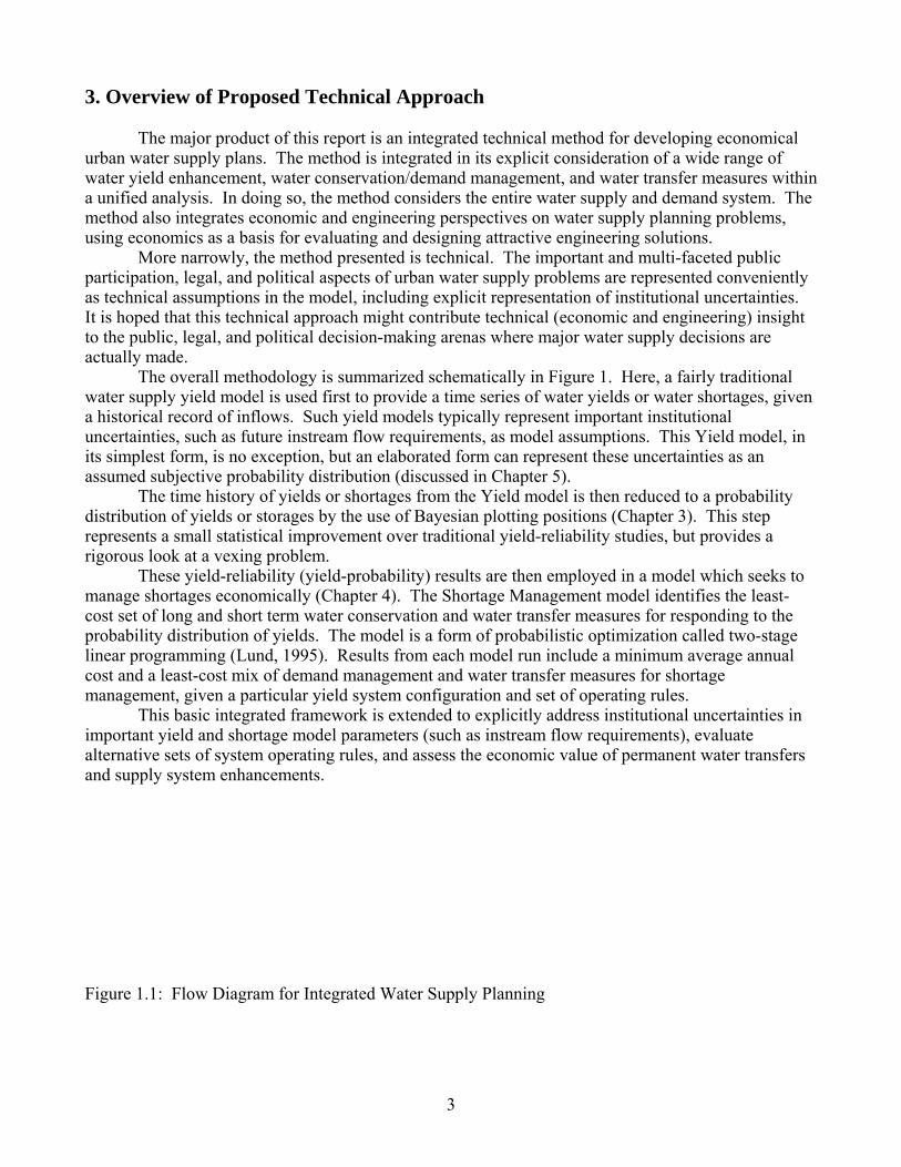
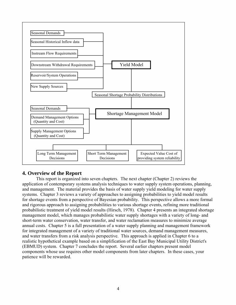
3. Overview of Proposed Technical Approach The major product of this report is an integrated technical method for developing economical urban water supply plans. The method is integrated in its explicit consideration of a wide range of water yield enhancement, water conservation/demand management, and water transfer measures within a unified analysis. In doing so, the method considers the entire water supply and demand system. The method also integrates economic and engineering perspectives on water supply planning problems, using economics as a basis for evaluating and designing attractive engineering solutions. More narrowly, the method presented is technical. The important and multi-faceted public participation, legal, and political aspects of urban water supply problems are represented conveniently as technical assumptions in the model, including explicit representation of institutional uncertainties. It is hoped that this technical approach might contribute technical (economic and engineering) insight to the public, legal, and political decision-making arenas where major water supply decisions are actually made. The overall methodology is summarized schematically in Figure 1. Here, a fairly traditional water supply yield model is used first to provide a time series of water yields or water shortages, given a historical record of inflows. Such yield models typically represent important institutional uncertainties, such as future instream flow requirements, as model assumptions. This Yield model, in its simplest form, is no exception, but an elaborated form can represent these uncertainties as an assumed subjective probability distribution (discussed in Chapter 5). The time history of yields or shortages from the Yield model is then reduced to a probability distribution of yields or storages by the use of Bayesian plotting positions (Chapter 3). This step represents a small statistical improvement over traditional yield-reliability studies, but provides a rigorous look at a vexing problem. These yield-reliability (yield-probability) results are then employed in a model which seeks to manage shortages economically (Chapter 4). The Shortage Management model identifies the least-cost set of long and short term water conservation and water transfer measures for responding to the probability distribution of yields. The model is a form of probabilistic optimization called two-stage linear programming (Lund, 1995). Results from each model run include a minimum average annual cost and a least-cost mix of demand management and water transfer measures for shortage management, given a particular yield system configuration and set of operating rules. This basic integrated framework is extended to explicitly address institutional uncertainties in important yield and shortage model parameters (such as instream flow requirements), evaluate alternative sets of system operating rules, and assess the economic value of permanent water transfers and supply system enhancements. Figure 1.1: Flow Diagram for Integrated Water Supply Planning

3

Yield Model

Seasonal Historical Inflow data

Instream Flow Requirements

Downstream Withdrawal Requirements

Reservoir/System Operations

New Supply Sources

Seasonal Shortage Probability Distributions

Shortage Management ModelSeasonal Demands

Demand Management Options(Quantity and Cost)

Supply Management Options(Quantity and Cost)

Long Term ManagementDecisions

Short Term ManagementDecisions

Expected Value Cost ofproviding system reliability

Seasonal Demands

4. Overview of the Report This report is organized into seven chapters. The next chapter (Chapter 2) reviews the application of contemporary systems analysis techniques to water supply system operations, planning, and management. The material provides the basis of water supply yield modeling for water supply systems. Chapter 3 reviews a variety of approaches to assigning probabilities to yield model results for shortage events from a perspective of Bayesian probability. This perspective allows a more formal and rigorous approach to assigning probabilities to various shortage events, refining more traditional probabilistic treatment of yield model results (Hirsch, 1978). Chapter 4 presents an integrated shortage management model, which manages probabilistic water supply shortages with a variety of long- and short-term water conservation, water transfer, and water reclamation measures to minimize average annual costs. Chapter 5 is a full presentation of a water supply planning and management framework for integrated management of a variety of traditional water sources, demand management measures, and water transfers from a risk analysis perspective. This approach is applied in Chapter 6 to a realistic hypothetical example based on a simplification of the East Bay Municipal Utility District's (EBMUD) system. Chapter 7 concludes the report. Several earlier chapters present model components whose use requires other model components from later chapters. In these cases, your patience will be rewarded.

4

Chapter 2 Urban Water Supply Planning and Management

"I shall now treat the ways in which water should be conducted to dwellings and cities. ..." Vitruvius (1st c. B.C., Book VIII, Chapter V) This chapter reviews the nature of urban water supply problems and the engineering and planning techniques that have been applied to them. The discussion begins with a review of the management measures available for urban water supply engineering, followed by a presentation of the sources of uncertainty involved in water supply planning, and concludes with a brief review of techniques applied to the engineering of management measures to create and sustain urban water supplies. The management measures available for urban water supply engineering can be divided into three broad categories. Water transfers or markets have received the most attention recently, while demand management or water conservation and yield enhancement are more traditional approaches taken to the problem. The following sections review each of these three categories of water supply management measures. 1. Water Transfers for Urban Water Supplies Use of Water Transfers in Urban Systems The integration of water transfers into urban water supply planning and management will be at least as complex a technical task as the still imperfect application of water conservation to urban systems. Some aspects of the use of water transfers in urban water supply planning and management are discussed by Lund, et al. (1992). There is a wide variety of water transfer types, listed in Table 2.1. Each type of water transfer has different operational and planning characteristics for urban supplies. The functions or uses of the many different forms of water transfers are summarized in Table 2.2. However, the integration of these many forms of water transfers into urban water supplies to serve multiple functions has received little attention (Lund, et al., 1992). Table 2.1: Major Types of Water Transfers Permanent Transfers Contingent Transfers/Dry-year Options Long-term Intermediate-term Short-term Spot Market Transfers Water Banks Transfer of Reclaimed, Conserved, and Surplus Water Water Wheeling or Water Exchanges Operational Wheeling Wheeling to Store Water Trading Waters of Different Qualities Seasonal Wheeling Wheeling to Meet Environmental Constraints

5

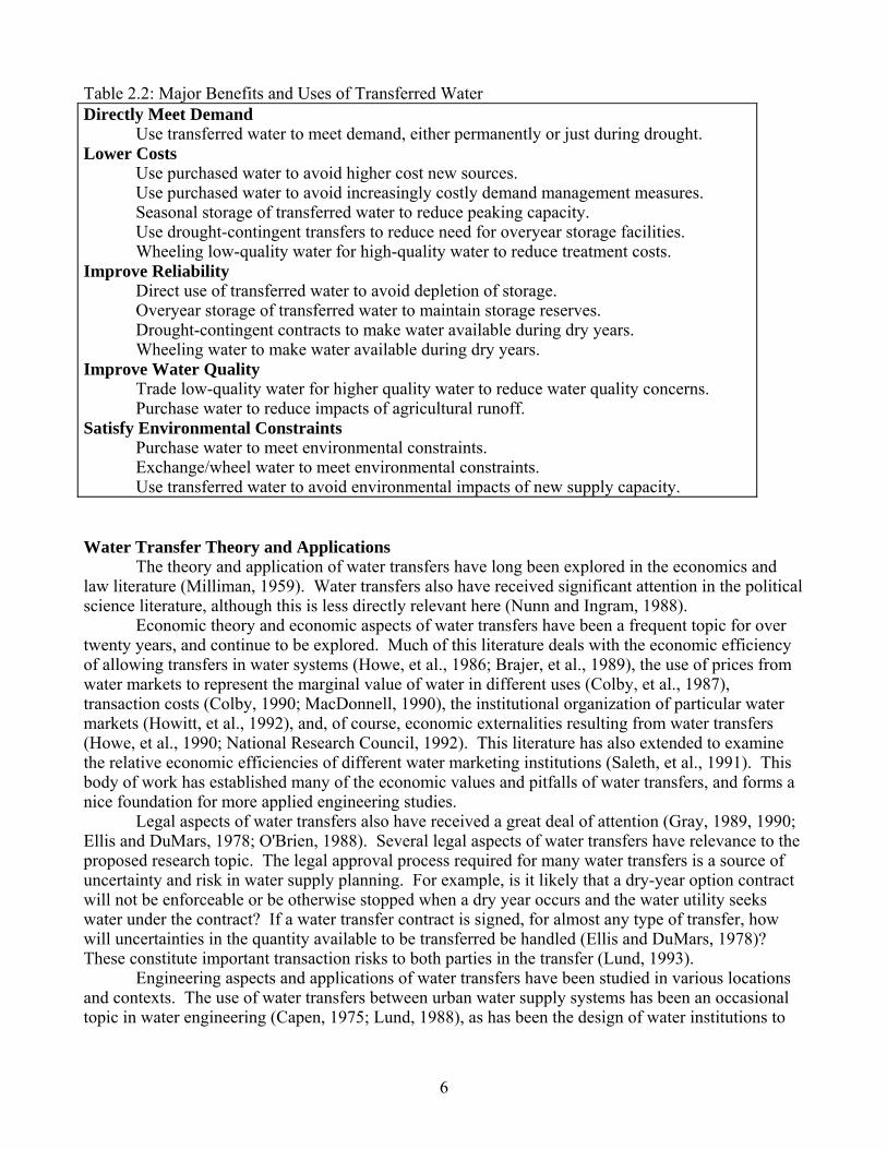
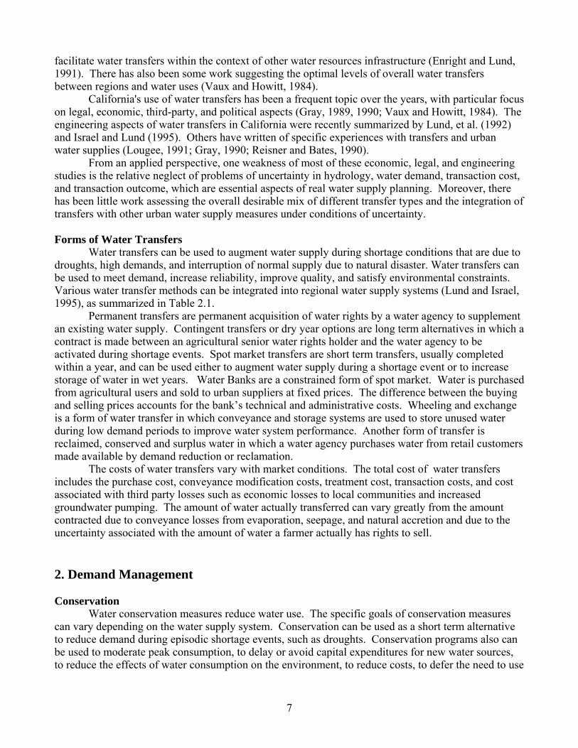
Table 2.2: Major Benefits and Uses of Transferred Water Directly Meet Demand Use transferred water to meet demand, either permanently or just during drought. Lower Costs Use purchased water to avoid higher cost new sources. Use purchased water to avoid increasingly costly demand management measures. Seasonal storage of transferred water to reduce peaking capacity. Use drought-contingent transfers to reduce need for overyear storage facilities. Wheeling low-quality water for high-quality water to reduce treatment costs. Improve Reliability Direct use of transferred water to avoid depletion of storage. Overyear storage of transferred water to maintain storage reserves. Drought-contingent contracts to make water available during dry years. Wheeling water to make water available during dry years. Improve Water Quality Trade low-quality water for higher quality water to reduce water quality concerns. Purchase water to reduce impacts of agricultural runoff. Satisfy Environmental Constraints Purchase water to meet environmental constraints. Exchange/wheel water to meet environmental constraints. Use transferred water to avoid environmental impacts of new supply capacity. Water Transfer Theory and Applications The theory and application of water transfers have long been explored in the economics and law literature (Milliman, 1959). Water transfers also have received significant attention in the political science literature, although this is less directly relevant here (Nunn and Ingram, 1988). Economic theory and economic aspects of water transfers have been a frequent topic for over twenty years, and continue to be explored. Much of this literature deals with the economic efficiency of allowing transfers in water systems (Howe, et al., 1986; Brajer, et al., 1989), the use of prices from water markets to represent the marginal value of water in different uses (Colby, et al., 1987), transaction costs (Colby, 1990; MacDonnell, 1990), the institutional organization of particular water markets (Howitt, et al., 1992), and, of course, economic externalities resulting from water transfers (Howe, et al., 1990; National Research Council, 1992). This literature has also extended to examine the relative economic efficiencies of different water marketing institutions (Saleth, et al., 1991). This body of work has established many of the economic values and pitfalls of water transfers, and forms a nice foundation for more applied engineering studies. Legal aspects of water transfers also have received a great deal of attention (Gray, 1989, 1990; Ellis and DuMars, 1978; O'Brien, 1988). Several legal aspects of water transfers have relevance to the proposed research topic. The legal approval process required for many water transfers is a source of uncertainty and risk in water supply planning. For example, is it likely that a dry-year option contract will not be enforceable or be otherwise stopped when a dry year occurs and the water utility seeks water under the contract? If a water transfer contract is signed, for almost any type of transfer, how will uncertainties in the quantity available to be transferred be handled (Ellis and DuMars, 1978)? These constitute important transaction risks to both parties in the transfer (Lund, 1993). Engineering aspects and applications of water transfers have been studied in various locations and contexts. The use of water transfers between urban water supply systems has been an occasional topic in water engineering (Capen, 1975; Lund, 1988), as has been the design of water institutions to

6

facilitate water transfers within the context of other water resources infrastructure (Enright and Lund, 1991). There has also been some work suggesting the optimal levels of overall water transfers between regions and water uses (Vaux and Howitt, 1984). California's use of water transfers has been a frequent topic over the years, with particular focus on legal, economic, third-party, and political aspects (Gray, 1989, 1990; Vaux and Howitt, 1984). The engineering aspects of water transfers in California were recently summarized by Lund, et al. (1992) and Israel and Lund (1995). Others have written of specific experiences with transfers and urban water supplies (Lougee, 1991; Gray, 1990; Reisner and Bates, 1990). From an applied perspective, one weakness of most of these economic, legal, and engineering studies is the relative neglect of problems of uncertainty in hydrology, water demand, transaction cost, and transaction outcome, which are essential aspects of real water supply planning. Moreover, there has been little work assessing the overall desirable mix of different transfer types and the integration of transfers with other urban water supply measures under conditions of uncertainty. Forms of Water Transfers Water transfers can be used to augment water supply during shortage conditions that are due to droughts, high demands, and interruption of normal supply due to natural disaster. Water transfers can be used to meet demand, increase reliability, improve quality, and satisfy environmental constraints. Various water transfer methods can be integrated into regional water supply systems (Lund and Israel, 1995), as summarized in Table 2.1. Permanent transfers are permanent acquisition of water rights by a water agency to supplement an existing water supply. Contingent transfers or dry year options are long term alternatives in which a contract is made between an agricultural senior water rights holder and the water agency to be activated during shortage events. Spot market transfers are short term transfers, usually completed within a year, and can be used either to augment water supply during a shortage event or to increase storage of water in wet years. Water Banks are a constrained form of spot market. Water is purchased from agricultural users and sold to urban suppliers at fixed prices. The difference between the buying and selling prices accounts for the bank’s technical and administrative costs. Wheeling and exchange is a form of water transfer in which conveyance and storage systems are used to store unused water during low demand periods to improve water system performance. Another form of transfer is reclaimed, conserved and surplus water in which a water agency purchases water from retail customers made available by demand reduction or reclamation. The costs of water transfers vary with market conditions. The total cost of water transfers includes the purchase cost, conveyance modification costs, treatment cost, transaction costs, and cost associated with third party losses such as economic losses to local communities and increased groundwater pumping. The amount of water actually transferred can vary greatly from the amount contracted due to conveyance losses from evaporation, seepage, and natural accretion and due to the uncertainty associated with the amount of water a farmer actually has rights to sell. 2. Demand Management Conservation Water conservation measures reduce water use. The specific goals of conservation measures can vary depending on the water supply system. Conservation can be used as a short term alternative to reduce demand during episodic shortage events, such as droughts. Conservation programs also can be used to moderate peak consumption, to delay or avoid capital expenditures for new water sources, to reduce the effects of water consumption on the environment, to reduce costs, to defer the need to use

7

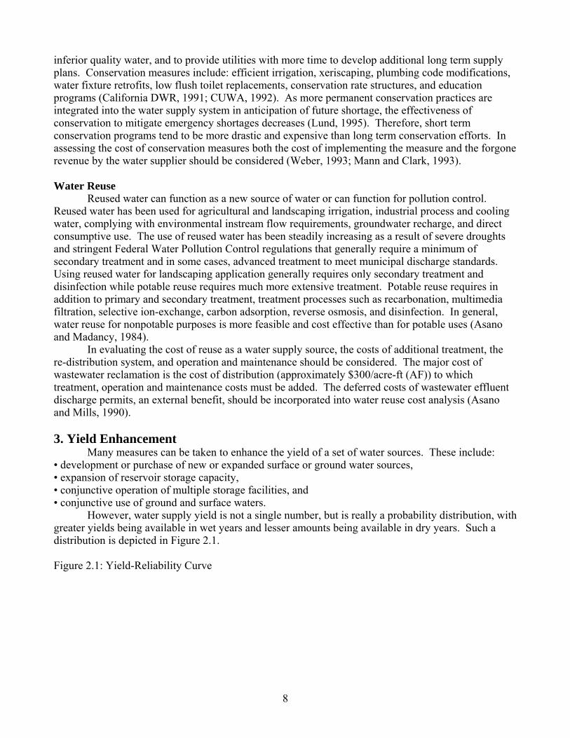
inferior quality water, and to provide utilities with more time to develop additional long term supply plans. Conservation measures include: efficient irrigation, xeriscaping, plumbing code modifications, water fixture retrofits, low flush toilet replacements, conservation rate structures, and education programs (California DWR, 1991; CUWA, 1992). As more permanent conservation practices are integrated into the water supply system in anticipation of future shortage, the effectiveness of conservation to mitigate emergency shortages decreases (Lund, 1995). Therefore, short term conservation programs tend to be more drastic and expensive than long term conservation efforts. In assessing the cost of conservation measures both the cost of implementing the measure and the forgone revenue by the water supplier should be considered (Weber, 1993; Mann and Clark, 1993). Water Reuse Reused water can function as a new source of water or can function for pollution control. Reused water has been used for agricultural and landscaping irrigation, industrial process and cooling water, complying with environmental instream flow requirements, groundwater recharge, and direct consumptive use. The use of reused water has been steadily increasing as a result of severe droughts and stringent Federal Water Pollution Control regulations that generally require a minimum of secondary treatment and in some cases, advanced treatment to meet municipal discharge standards. Using reused water for landscaping application generally requires only secondary treatment and disinfection while potable reuse requires much more extensive treatment. Potable reuse requires in addition to primary and secondary treatment, treatment processes such as recarbonation, multimedia filtration, selective ion-exchange, carbon adsorption, reverse osmosis, and disinfection. In general, water reuse for nonpotable purposes is more feasible and cost effective than for potable uses (Asano and Madancy, 1984). In evaluating the cost of reuse as a water supply source, the costs of additional treatment, the re-distribution system, and operation and maintenance should be considered. The major cost of wastewater reclamation is the cost of distribution (approximately $300/acre-ft (AF)) to which treatment, operation and maintenance costs must be added. The deferred costs of wastewater effluent discharge permits, an external benefit, should be incorporated into water reuse cost analysis (Asano and Mills, 1990). 3. Yield Enhancement Many measures can be taken to enhance the yield of a set of water sources. These include: • development or purchase of new or expanded surface or ground water sources, • expansion of reservoir storage capacity, • conjunctive operation of multiple storage facilities, and • conjunctive use of ground and surface waters. However, water supply yield is not a single number, but is really a probability distribution, with greater yields being available in wet years and lesser amounts being available in dry years. Such a distribution is depicted in Figure 2.1. Figure 2.1: Yield-Reliability Curve

8

Annual Yield (TAF)

Percent of Time at or Above Yield

Firm Yield

100 0

Max Yield

Changes can be made in the operation policies of storage facilities and sources to change the relative likelihood (probability distribution) of different yields being available. For example, through the use of "hedging" reservoir releases, small shortages can be made more frequent while reducing the frequency of large shortages. Assessment of the yield of a set of water sources typically requires the use of computer models, most typically simulation models, although optimization models can also have a role. There are many simulation and optimization models that aid the examination of water source operation and planning problems. State-of-the-art reviews of reservoir management and operations models have been presented by Yeh (1985) and Wurbs et al. (1991, 1993) and provide extensive lists of references. The following two sections review key examples of simulation and optimization models for various types of yield studies. Simulation Models of Water Supply Yield Simulation models have been created for many specific reservoir systems. The Colorado River Simulation Model (CRSM) is an example of a river basin specific simulation model. The CRSM, a component of the Colorado River Simulation System (CRSS), is a deterministic simulation model developed by the Bureau of Reclamation for maintaining storage levels in Lake Powell and Lake Mead in accordance with the “Laws of the River”. It is used to model proposed modifications to the river system operation and study their effects on the quantity and quality of water in the river. The model is based on monthly time steps and on meeting end-of-month storage targets (Cowan et al, 1981). Some simulation models attempt to be more general and can be applied to various system configurations and objectives. For example, HEC-5 is a general simulation model applied to a wide variety of systems. HEC-5 was developed by the Army Corps of Engineers and provides monthly, daily, and hourly simulation of reservoir operation and stream flow routing through a network of conveyance and storage systems. It is used mainly for hydropower and flood control objectives (Feldman, 1981). STELLA (Systems Thinking Experimental Learning Laboratory with Animation) is an interactive graphically oriented program designed to aide in constructing dynamic systems simulation models. Karpack and Palmer (1992) used STELLA to develop simulation models for the Seattle and Tacoma, Washington water supply systems and evaluate the potential value of an intertie between the two major water suppliers. The graphical environment and user interface allowed rapid construction of the models, great flexibility, high quality graphical presentation, and the potential for non-programmers to understand the model contents and assumptions. ResQ is an interactive single reservoir operation simulation model designed for microcomputer use. The program has four components: data acquisition, management and processing, analysis model, and interface with the user.

9

The analysis model is based on a recursive continuity equation and can be used either to determine suitable operating rules to meet specified demands or to determine the effects of specific operation rules on the yield (Ford, 1990). Spreadsheet programs such as Excel have been used for relatively simple reservoir-analysis simulation models. Yield simulation models can provide estimates of shortage event probabilities given assumptions about water use, system configuration, and operating rules of the system. The GRAM (General Risk Analysis Model) developed by Hirsch (1978) was applied to the Occoquan Reservoir to estimate a set of shortage emergency probabilities. The produced shortage probability distribution can be used by water system managers to better understand their system’s reliability, estimate system yield, and reform operating rules to improve system reliability. Simulation models also can be used in conjunction with optimization. WASP is an integrated simulation and optimization model for a range of water supply systems without hydropower. It uses a network linear programming formulation to find the minimum penalty seasonal water assignments and then simulates the linear programming allocation with the guidance of given operating rules. Three operating rules are available to the user: resource target curves, demand restriction rules, and reservoir target curves. The model was used to model the Melbourne Water Supply System and determine efficient water balance scenarios (Kuczera and Diment, 1988). DWRSIM is a sequential use of simulation and optimization for modeling the optimal delivery schedule to deliver excess delta water from the California State Water Project to Southern California (Chung and Helweg, 1985). Optimization Models of Water Supply Yield Management and operation of an urban water supply system has become a complex task requiring careful planning. Optimization models have been developed to assist in this challenge and to better understand urban water supply system behavior. Previous optimization models considered capacity enhancement and options to augment water supply based on physical and timing constraints. Butcher, et al. (1969) used a dynamic programming model to determine the construction sequence of additional system capacity based solely on increasing demand. The model assumed that total proposed capacity equaled demand at the end of the planning period. The model accounted for the effects of discount rate, increasing demand, and the cost per unit supply available from each source. Morin and Esogbue (1971) modified the model presented by Butcher et al. by allowing a subset of available projects to be scheduled and developed a more general selection and sequencing model. Neither model accounted for variability in the existing water supply and the ability to manage demand. The total cost of the preferred alternatives was based solely on the construction costs. Other optimization models explored the ability to increase system reliability with system operations. Palmer and Holmes (1988) developed an expert system for water managers for reservoir operation under drought conditions. The expert system approach integrated a series of rules and facts based on operators’ experience and an optimization program to determine system yield and optimal operating policy. The expert system provided the user with either general drought potential information or detailed recommendations for a specific action based on results from historical drought events and inflows. Randall, et al. (1990) developed a multi-objective program to study water supply system operation during droughts. The objectives of the program included maximizing net revenues and reliability and meeting end of planning period storage and streamflow requirements. The program was used to develop a revenue-reliability trade-off curve for system operations. The study's trade-off curve results indicated that significant additional system reliability could be obtained with a relatively small decrease in revenues. Shih and ReVelle (1995) presented a mixed integer programming model to determine triggers, measured as the reservoir storage volumes plus inflow, for rationing. The objectives of the model were to maximize the number of days without drought and to minimize the number of extreme drought events. The model showed that trigger volumes are sensitive to the

10

number of extreme events allowed. As tolerance for extreme events decreased, the number of small shortage events and the trigger volume value for those events increased. 4. Uncertainties in Water Supply Planning Uncertainties in environmental regulations, demand, and hydrological forecasts can greatly affect urban water supplies. Hydrologic Uncertainty Hydrologic uncertainty arises from the annual and seasonal variability in rainfall, snowfall, evaporation, snowmelt, and, ultimately, runoff. Traditional water resources planning has focused almost exclusively on hydrologic uncertainty in water supply yield (Rippl, 1883; Vogel, et al., 1995). Thus, the effects of hydrologic uncertainty on water system yield are rather well understood. Hydrologic uncertainty also can have considerable effects on water demands (especially where rain-fed lawn watering or "dryland" farming are common) and the ability to complete water transfers, issues of potentially great importance for contemporary urban water supplies. For water transfers, hydrologic uncertainties affect the availability of water for transfer (also affecting its spot-market price) and the availability of existing and other alternative water supplies (in wet years, transfers may be unneeded). For dry year options, hydrologic uncertainty might affect the availability of water from suppliers with relatively junior water rights. Water Demand Uncertainties Water demand uncertainties exist in the long term due to uncertainties in the growth of urban regions, future use of water-using technologies, future plumbing codes and land-use regulations, etc. There is also a degree of short-term uncertainty in urban water demands due to variation in weather patterns. Uncertainty in agricultural water demands may also affect the price and amount of water available for transfer to urban users or the withdrawals of senior agricultural water users. Agricultural water demand is subject to variations in weather patterns, changes in agricultural product prices and subsidies, changes in environmental regulations, and other factors. These uncertainties can have significant impacts on system performance (Ng and Kuczera, 1993). Institutional Uncertainties for Water Yield There is considerable uncertainty at planning and sometimes operational time-scales regarding minimum instream flow requirements, water demands of senior water right holders, and other institutional considerations which affect the water supply yield of a water supply system. These uncertainties typically are considered by making single-valued assumptions for these parameters in system yield models. Transaction Uncertainties for Water Transfers Uncertainty in the ability to successfully negotiate and implement a proposed water transfer (transaction risk) arises due to legal, economic, environmental, logistic, or other potential obstacles. Several recent proposed water transfers in California have fallen victim to this source of uncertainty, after considerable expense (SWRCB, 1988). Spot market transfers usually require quick negotiation of prices and terms within a tight schedule of crop planting and irrigation scheduling decisions. Theoretical aspects of transaction risk are discussed by Lund (1993). Uncertainty in the delivery of transferred water arises from the uncertain magnitude of losses of transferred water in the course of the conveyance, storage, and treatment required to physically utilize water which has been legally transferred. Many water transfers may be subject to significant losses of

11

legally transferred water through the operation of water resources infrastructure (Lougee, 1991; Lund, et al., 1992). The quantity of these losses may be somewhat uncertain before the transfer has been completed. In addition, there may also be losses of water due to uncertainty in the quantification of the water rights which are the basis for a water transfer (Ellis and DuMars, 1978). 5. Traditional Water Supply Engineering Traditionally, water supply engineering was based on a "requirements" approach. The water supply "needs" of a service area typically were estimated based on per-capita "requirements" and this was multiplied by an estimated or projected service area population. This total water demand "requirement" was then sought from a supply system. One or more water sources would be evaluated in terms of their individual and combined "firm yields". The "firm yield" is the highest yield from a source which can be sustained during the worst drought of record, found by the Rippl method (1883) still presented in current text-books (Linsley, et al., 1992). This supply was assumed to be "firm" and was sometimes assumed to be "safe". While this planning approach is simple, expedient, and serves well in many situations well, the approach's limitations are evident. While forecasting is always difficult, it was common for the simple water demand forecasts to be grossly in error and based on unrealistic projections of both population and future per-capita water use (Lund, 1988a, 1988b). Single-valued demand estimates also ignore the flexibility of water demands in the face of shortages. The estimation of yield as a single number also had evident problems. Usually a source provides more water than the firm yield, and as development of new sources became increasingly expensive and demands grew, firm yield became overly expensive and difficult to provide. Basing design on the "worst drought of record" also became somewhat difficult to defend. As years pass, new droughts occur, raising the possibility of lower "firm yields" as the record length increases. Basing design on a system's "firm yield" became increasingly seen as a very expensive and inflexible way of avoiding even the smallest and least expensive shortages (Russell, et al., 1970). 6. Contemporary Water Supply Engineering Water supply planning has become more sophisticated since the 1960s. Water demands are presently made using better researched and often more sophisticated forecasting methods. While forecasts are still subject to important errors, they are far more reliable and are used with more sophistication and caution. Typically, various water demand scenarios are evaluated, reflecting optimistic, pessimistic, and expected demographic, economic, and water use assumptions. Water demands also are considered to be more flexible through the use of water conservation or demand management measures. Drought or shortage management strategies have become an explicit and well-developed part of most urban water supply plans (California DWR, 1991; CUWA, 1992). Yield modeling and source management also have become much more sophisticated. Computer models are used to investigate a wider range of potential water source configurations and operations, with yield-reliability studies becoming common. Some qualitative attempts are usually made to find a promising match between measures which enhance yield reliability and those which reduce or modify water demands. Almost all modeling done for these purposes is simulation modeling, with simulation and sometimes forecast models tailored to specific water supply systems. While these innovations in water supply planning have greatly improved the management of these systems and widened the range of alternatives that are considered, the integration of available water management measures into working systems has been accomplished largely in an informal way. Throughout the years, academic advice has been given to formalize various aspects of water supply

12

planning. In many cases, this advice eventually has become applied widely with great success (Howe and Linaweaver, 1967; Maass, et al., 1966). 7. Academic Advice Traditional "systems analysis" of water supplies is well developed (Maass, 1962; Loucks, Stedinger, and Haith, 1981; Yeh, 1985; Mays and Tung, 1992). It includes many forms of simulation and optimization modeling for improving the yield or minimizing the losses from operating single and multiple reservoir systems. These models range over a wide variety of both deterministic and probabilistic formulations. In recent decades, water supply problems have evolved to require the engineering of new forms of water storage, such as groundwater storage, the conjunctive use of ground and surface water storage, and the use of off-stream surface water storage. Traditional systems analysis, based primarily on on-stream surface water reservoirs, has been extended to include a wide variety of applications to these more complex systems (Willis and Yeh, 1987; Buras, 1965). As new water supply sources become scarce or infeasible, and their marginal costs increase, water managers explore the use of demand curbing or shaping management options in anticipation of water shortages. This expanded range of planning alternatives, in turn, has been incorporated into systems analysis of urban water supplies (Lund, 1987; Rubenstein and Ortolano, 1984; Dziegielewski and Crews, 1986). Several optimization models reflect the trend of incorporating conservation and demand management into water supply system management. Lund (1987) used a sequential linear programming method to evaluate and schedule water conservation measures for either avoiding or deferring capacity expansion to minimize costs. When capacity expansion was not required, conservation measures were scheduled if the annualized costs of conservation were less than the resulting annualized reduction in system operation and maintenance costs. When capacity expansion was expected, conservation measures were scheduled to most efficiently delay the expansion. Rubenstein and Ortolano (1984) formulated a dynamic programming algorithm to develop an efficient use of water resources by considering demand management options to supplement limited available water sources. The dynamic program algorithm had two weighted objective functions that were solved separately and then combined. The first objective function determined the minimum expected value of new construction project costs while the second objective function determined the minimum expected value of emergency plans during drought events. The problem was solved for different emergency scenarios each having a distinct magnitude, duration, and frequency. Their results showed that significant water savings can be attained by managing demand and that the formulation enabled the user to identify the trade-off between long term measures and short term measures. There has been some work using systems analysis to assess optimal levels of inter-regional water transfers (Vaux and Howitt, 1984). However, the integrated planning of traditional water sources, water conservation, and water transfers using systems analysis has received little attention (Lund and Israel, 1995). 8. "Integrated Resource Planning" In recent years, the term "integrated resource planning" or "IRP" has become popular for characterizing the need for, and approaches towards, a more comprehensive planning and management of water supplies (JAWWA, 1995). While use of the term "IRP" has reached a fever pitch in the consulting world, considerable variation in what is being "integrated" is evident in such studies. Attempts at the following forms of integration are sometimes evident from the literature and

13

presentations of IRP applications to water supply problems: 1. Integration of yield improvement, demand management, and water transfer measures in water supply planning. 2. Integration of planning for multiple resources. Here, water, wastewater, and sludge management might together be the subject of an "integrated" resource plan. 3. Integration of multiple water uses in water planning. Thus, recreational, hydropower, environmental, and multiple water supply uses of a set of water resources might be planned together, in a way similar to traditional multi-purpose water resources planning. 4. Integration of the technical planning process into a social and political context. This form of integration typically strives to improve the prospects for implementing the results of a relatively technical planning process by increased public participation or "consensus-building" in the planning process. 5. Integration of multiple sources of water and their operation for improving supply system yield. This is the most limited, though technically still challenging and important, use of the term "Integrated Resource Planning". Another distinction of "integrated" resource planning approaches is that they often attempt to make increased use of probabilistic risk assessment, compared to traditional and most contemporary water supply planning applications. Thus, water supply yield and future water demands are more often seen as being probabilistic. This is a technically difficult endeavor and one which, as shown in later chapters, becomes more interesting as attempts are made to "integrate" various uncertainties in a formal technical planning process. While the call to comprehensiveness, explicit in much of the IRP literature and practice, is philosophically attractive, its technical and procedural difficulties are formidable. The chapters which follow are an attempt to provide a comprehensive technical approach to the integrated resource management of urban water supply systems. This technical approach, previewed in Chapter 1, most closely follows the first (and fifth) definitions of "integrated" planning above, but could (and indeed should often) be extended or incorporated into a larger planning framework to address other uses of the term "integrated." However, before an "integrated" approach can be presented, the individual pieces of the problem must be prepared. The next chapter (Chapter 3) is devoted to the rather narrow topic of assigning probability values to water supply yield or shortage levels, based on the results of traditional water supply yield models employing historical unimpaired streamflows (discussed in Chapter 2). Chapter 4 follows with presentation of a Shortage Management Model to represent the demand side of the system. Chapter 5 presents the formal integration of yield and shortage management models, which is applied to the EBMUD system in Chapter 6.

14

Chapter 3 Plotting Positions for Water Supply Reliability

1. Introduction Formal estimation of water supply shortage probabilities is becoming more widespread in engineering practice. Most commonly, this is done by assigning a probability plotting position to each result of a system simulation model which employs historical inflows to represent uncertainty in future streamflows. This chapter compares alternative approaches to assigning probability plotting positions to such model results (shortages, costs, yields) and discusses formal approaches to examining the reliability of such probability estimates. The chapter also discusses the problem of assigning probabilities where shortages are scarce and compares the economic and decision-making implications of alternative plotting position formulae. The overall intent of this chapter is to explore the assignment of exceedence probabilities to the time series of yields or shortages produced by yield models such as those most commonly employed for water supply system studies. In trying to assess the need for new water supplies or increased demand management, water supply engineers increasingly have gone beyond firm yield studies to more formal estimations of yield and shortage probabilities. Such studies are typically based on system simulation model results, based on the historical streamflow record. A major technical problem in such an exercise is the assignment of formal probability values to the shortage amounts appearing in the simulation results, a problem somewhat similar to selecting a plotting position formula for flood studies. There is considerable uncertainty inherent in the estimates of the probability of simulated yield or shortage results based on short (<100 years) hydrologic records (Pretto, et al., 1997). This chapter examines alternative plotting positions for such simulation model results, comparing several commonly employed and other plotting position formulae from the perspective of Bayesian inference. Explicit Bayesian analysis is undertaken to assess the probability distribution of non-exceedence probabilities for specific yield or shortage levels. Significant changes in the shape of yield or shortage probability distributions can result from the different sets of system configurations and operating rules commonly explored in yield reliability studies. Thus, it seems inappropriate to base probability plotting positions for supply-system yield on an assumed distributional form. This situation contrasts with the use of plotting positions for flood flows, where assumed distributional forms are available to guide selection of a plotting position formula (Cunnane, 1978). An alternative approach, obviating the need for plotting position formulae for water supply, is the use of synthetic hydrologies (Salas, et al., 1988; Vogel and Bolognese, 1995). The use of synthetic hydrology allows large amounts of yield data to be generated; under these conditions the probability assignment problem for a given level of yield is merely the number of exceedences divided by the number of synthetic "observations". However, this approach has not found widespread acceptance in the practicing profession and retains some academic skepticism. This chapter proceeds with a short discussion of desirable features for plotting position formulae for water supply problems, followed by presentation of a Bayesian approach to examining the plotting position problem. A Bayesian plotting position formula (Jaynes, 1996; Jeffreys, 1961) is presented for a uniform prior (having minimum prior information content). Comparisons are then made of the prior distributions implied by some common plotting position formulae, including examination of the Bayesian uncertainty in posterior estimates of exceedence probabilities. A planning example is then briefly examined to ascertain if selection of a plotting position formula is of

15

practical economic and decision-making importance. The chapter concludes with a discussion of the limitations of the Bayesian approach and some conclusions. 2. Desirable Features of Plotting Position Formulae Several features are desirable for plotting position formulae for water supply reliability studies. Exceedence probability plotting positions for event i, pi, being the ri-th largest event of n-simulated observations, should: 1. Converge to pi = ri/n, for large n. This follows from the Law of Large Numbers. 2. Allow for events larger and smaller than those seen so far, especially for small n. For almost any historical hydrologic record, it is likely that the "worst" circumstances of record are not likely to produce the worst possible system yields or shortages. 3. Provide a probabilistic indication of uncertainty in the estimated exceedence probability. Instead of merely indicating the exceedence probability of event i, it is desirable to have an explicit estimate of P(pi|ri,n), representing the probability distribution of pi, given the observed or simulated data. 4. Provide the expected value of the probability distribution of exceedence probability for an event i. For any value of ri and n, the exceedence probability for planning and decision-making purposes should be pi = P(s>si) = EV(P(s>si)|ri,n) (Howard, 1988), where s is the magnitude of a shortage or yield event. 5. Be relatively distribution-free. For water supply problems involving the operation of reservoirs and multiple water sources, it is unlikely that the probability distribution of yield or shortage will follow any fixed frequency distribution, as is often successfully assumed with flood frequency problems (Cunnane, 1978). Therefore, it seems desirable not to have plotting position formula selection based on frequency distribution assumptions. The Bayesian approach to developing plotting position formulae for water supply reliability planning presented here provides plotting position formulae which satisfy these criteria fairly well. 3. Bayesian Derivation of Plotting Positions Several authors have applied Bayesian probabilities to the development of plotting positions (Jaynes, 1996; Epstein, 1985; Box and Tiao, 1973; Hirsch, 1978). These approaches begin by considering the probability distribution of an exceedence probability for a yield or shortage event i. Without observations, the exceedence probability of a given level of event is highly uncertain. The uncertainty of these situations is represented by the probability distribution of the exceedence probability of event i, P(pi), the prior in Bayesian analysis. This prior probability distribution is represented variously by different authors. Bayes Theorem is then applied to use data to update this prior distribution,

(1) P(pi|ri,n) = P(ri|pi,n) P(pi)

⌡⌠0

1P(ri|pi,n)dpi

= P(ri|pi,n) P(pi)

P(ri|n) ,

where ri is the number of occurrences exceeding shortage event i observed in n observations. The denominator P(ri|n) is a constant, not varying with pi, and so can be solved later as a scaling constant to ensure

16

(2) ⌡⌠-∞

∞P(pi|ri,n) dpi = 1.

P(ri|pi,n) is the likelihood function, indicating the probability of ri exceedences out of n trials, given that pi is the known probability of exceedence. With this interpretation and the assumption that exceedences of shortage event i are independent (a Bernoulli process), P(ri|pi,n) is a binomial distribution, (3) P(ri|pi,n) = piri (1-pi)n-ri. The posterior distribution of the exceedence probability, P(pi|ri,n), then varies with the interaction of the above binomial distribution and the prior distribution P(pi). The posterior distribution, in this case, is the probability distribution of the probability of exceeding event i, given both the prior distribution and observing that this event was exceeded ri times out of n observations. For a wide variety of prior probability distributions, the conjugate posterior distribution is a Beta distribution:

(4) P(pi|ri,n) = piai-1 (1-pi)bi-1

B(ai,bi) ,

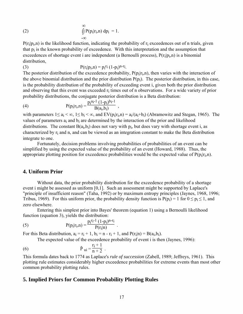
with parameters 1≤ ai < ∞, 1≤ bi < ∞, and EV(pi|ri,n) = ai/(ai+bi) (Abramowitz and Stegan, 1965). The values of parameters ai and bi are determined by the interaction of the prior and likelihood distributions. The constant B(ai,bi) does not vary with pi, but does vary with shortage event i, as characterized by ri and n, and can be viewed as an integration constant to make the Beta distribution integrate to one. Fortunately, decision problems involving probabilities of probabilities of an event can be simplified by using the expected value of the probability of an event (Howard, 1988). Thus, the appropriate plotting position for exceedence probabilities would be the expected value of P(pi|ri,n). 4. Uniform Prior Without data, the prior probability distribution for the exceedence probability of a shortage event i might be assessed as uniform [0,1]. Such an assessment might be supported by Laplace's "principle of insufficient reason" (Taha, 1992) or by maximum entropy principles (Jaynes, 1968, 1996; Tribus, 1969). For this uniform prior, the probability density function is P(pi) = 1 for 0 ≤ pi ≤ 1, and zero elsewhere. Entering this simplest prior into Bayes' theorem (equation 1) using a Bernoulli likelihood function (equation 3), yields the distribution:

(5) P(pi|ri,n) = piri-1 (1-pi)n-ri

P(ri|n) .

For this Beta distribution, ai = ri + 1, bi = n - ri + 1, and P(ri|n) = B(ai,bi). The expected value of the exceedence probability of event i is then (Jaynes, 1996):

(6) P- ui = ri + 1n + 2 .

This formula dates back to 1774 as Laplace's rule of succession (Zabell, 1989; Jeffreys, 1961). This plotting rule estimates considerably higher exceedence probabilities for extreme events than most other common probability plotting rules. 5. Implied Priors for Common Probability Plotting Rules

17

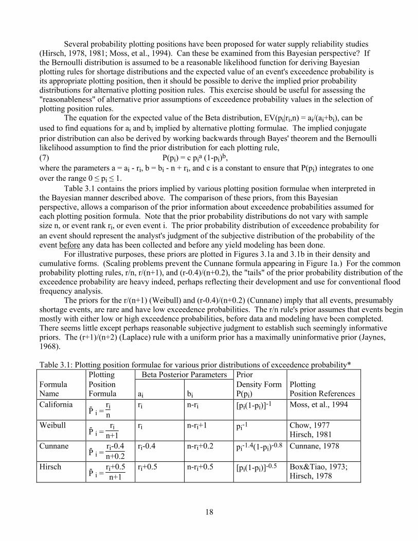
Several probability plotting positions have been proposed for water supply reliability studies (Hirsch, 1978, 1981; Moss, et al., 1994). Can these be examined from this Bayesian perspective? If the Bernoulli distribution is assumed to be a reasonable likelihood function for deriving Bayesian plotting rules for shortage distributions and the expected value of an event's exceedence probability is its appropriate plotting position, then it should be possible to derive the implied prior probability distributions for alternative plotting position rules. This exercise should be useful for assessing the "reasonableness" of alternative prior assumptions of exceedence probability values in the selection of plotting position rules. The equation for the expected value of the Beta distribution, EV(pi|ri,n) = ai/(ai+bi), can be used to find equations for ai and bi implied by alternative plotting formulae. The implied conjugate prior distribution can also be derived by working backwards through Bayes' theorem and the Bernoulli likelihood assumption to find the prior distribution for each plotting rule, (7) P(pi) = c pia (1-pi)b, where the parameters a = ai - ri, b = bi - n + ri, and c is a constant to ensure that P(pi) integrates to one over the range 0 ≤ pi ≤ 1. Table 3.1 contains the priors implied by various plotting position formulae when interpreted in the Bayesian manner described above. The comparison of these priors, from this Bayesian perspective, allows a comparison of the prior information about exceedence probabilities assumed for each plotting position formula. Note that the prior probability distributions do not vary with sample size n, or event rank ri, or even event i. The prior probability distribution of exceedence probability for an event should represent the analyst's judgment of the subjective distribution of the probability of the event before any data has been collected and before any yield modeling has been done. For illustrative purposes, these priors are plotted in Figures 3.1a and 3.1b in their density and cumulative forms. (Scaling problems prevent the Cunnane formula appearing in Figure 1a.) For the common probability plotting rules, r/n, r/(n+1), and (r-0.4)/(n+0.2), the "tails" of the prior probability distribution of the exceedence probability are heavy indeed, perhaps reflecting their development and use for conventional flood frequency analysis. The priors for the r/(n+1) (Weibull) and (r-0.4)/(n+0.2) (Cunnane) imply that all events, presumably shortage events, are rare and have low exceedence probabilities. The r/n rule's prior assumes that events begin mostly with either low or high exceedence probabilities, before data and modeling have been completed. There seems little except perhaps reasonable subjective judgment to establish such seemingly informative priors. The (r+1)/(n+2) (Laplace) rule with a uniform prior has a maximally uninformative prior (Jaynes, 1968). Table 3.1: Plotting position formulae for various prior distributions of exceedence probability* Plotting Beta Posterior Parameters Prior Formula Name

Position Formula

ai

bi

Density Form P(pi)

Plotting Position References

California P- i =

rin

ri n-ri [pi(1-pi)]-1 Moss, et al., 1994

Weibull P- i =

rin+1

ri n-ri+1 pi-1 Chow, 1977 Hirsch, 1981

Cunnane P- i =

ri-0.4n+0.2

ri-0.4 n-ri+0.2 pi-1.4(1-pi)-0.8 Cunnane, 1978

Hirsch P- i =

ri+0.5n+1

ri+0.5 n-ri+0.5 [pi(1-pi)]-0.5 Box&Tiao, 1973; Hirsch, 1978

18

Laplace P- i =

ri+1n+2

ri+1 n-ri+1 1 (Uniform) Laplace, 1774; Jeffreys, 1961

*Each prior form must be multiplied by a suitable scaling constant (which varies with ri and n, but not pi) to assure its integration to one over the range of 0 ≤ pi ≤ 1.

19

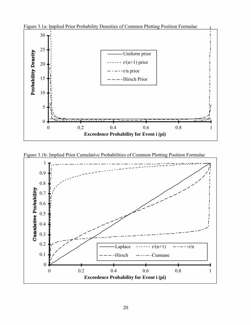
Figure 3.1a: Implied Prior Probability Densities of Common Plotting Position Formulae

0

5

10

15

20

25

30

0 0.2 0.4 0.6 0.8 1Exceedence Probability for Event i (pi)

Uniform prior

r/(n+1) prior

r/n prior

Hirsch Prior

Figure 3.1b: Implied Prior Cumulative Probabilities of Common Plotting Position Formulae

0

0.1

0.2

0.3

0.4

0.5

0.6

0.7

0.8

0.9

1

0 0.2 0.4 0.6 0.8 1Exceedence Probability for Event i (pi)

Laplace r/(n+1) r/n

Hirsch Cunnane

20

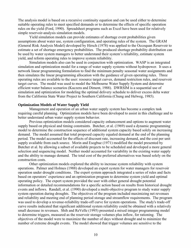
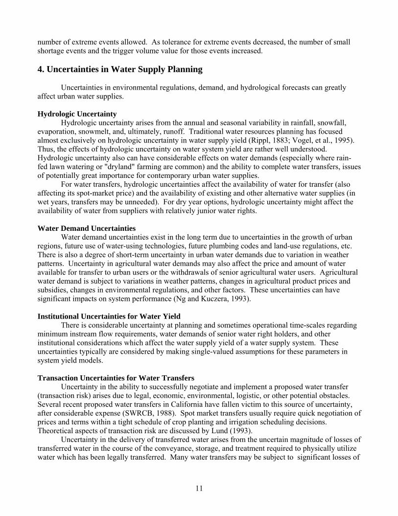
6. Comparison of Formulae Results This section provides a comparison of the different posterior distributions of exceedence probability and the expected value (mean) exceedence probability resulting from each of the above prior probability distributions. These results all stem from the Beta distribution in Equation 4, with the appropriate values of ai and bi for each plotting position formula's implied prior distribution (Table 3.1). Figure 3.2 below shows the posterior probability distributions of the exceedence probability of the worst yield level observed for a system simulation over a 50-year record for each of the prior probability distributions associated with the plotting position formulae discussed above (r=1, n=50). The expected value for each of these distributions of exceedence probabilities is the plotting position. These Beta distributions are a probabilistic representation of the uncertainty of the exceedence probability of this worst event, given the different prior distributions. The effects of increased amounts of data on the uncertainty in the exceedence probability is shown by comparing Figure 3.2 with Figure 3.3, with four times as much data, keeping r/n constant so that r=4 and n=200 in Figure 3.3. For this case, assuming both sets of r and n represent the same shortage or yield level, there is considerably less uncertainty in the event's exceedence probability with more data (n=200). There is also much greater agreement between the various probability plotting formulae and much less importance attached to their prior probability distributions. As is natural with Bayesian methods, larger samples tend to dampen the importance of the prior probability distribution. Perhaps more importantly, Table 3.2 shows the different plotting positions (expected values of the respective posterior Beta distributions) for different record lengths with the same ratio of r/n = 0.02. These are the probability values that would and should be used for evaluations of planning and management decisions regarding these ranked events (Howard, 1988). The first case in Table 2 (r=1, n=50) is not unrealistic for many extreme events from the historical record in a water supply planning context. There seems little likelihood that r/n and r/(n+1) plotting position results have any practical difference. However, there are greater and potentially important differences with other plotting formulae, with the Cunnane formula ((r-0.4)/(n+0.2)) resulting in a probability over one third less than the maximum result obtained from assuming a uniform prior or Laplace rule ((r+1)/(n+2)). A later section examines if these differences are important economically or for planning and management decision-making. The final lesson from Table 3.2 is that all plotting formulae converge to r/n, albeit at somewhat different rates, as can be seen moving across the table. With 500 years of data and r/n = 0.02, there is about a 10% range of expected exceedence probabilities, compared with a range of over 300% for the first case (r=1, n=50). Again, additional data reduces the importance of the prior distribution of exceedence probabilities, as represented in the plotting position formulae. Table 3.2: Expected Values of Exceedence Probabilities for Various cases where r/n = 0.02

r: 1 2 3 4 5 6 10 n: 50 100 150 200 250 300 500

r/n 0.0200 0.0200 0.0200 0.0200 0.0200 0.0200 0.0200 r/(n+1) 0.0196 0.0198 0.0199 0.0199 0.0199 0.0199 0.0200 (r-0.4)/(n+0.2) 0.0120 0.0160 0.0173 0.0180 0.0184 0.0187 0.0192 (r+0.5)/(n+1) 0.0294 0.0248 0.0232 0.0224 0.0219 0.0216 0.0210 (r+1)/(n+2) 0.0385 0.0294 0.0263 0.0248 0.0238 0.0232 0.0219

21

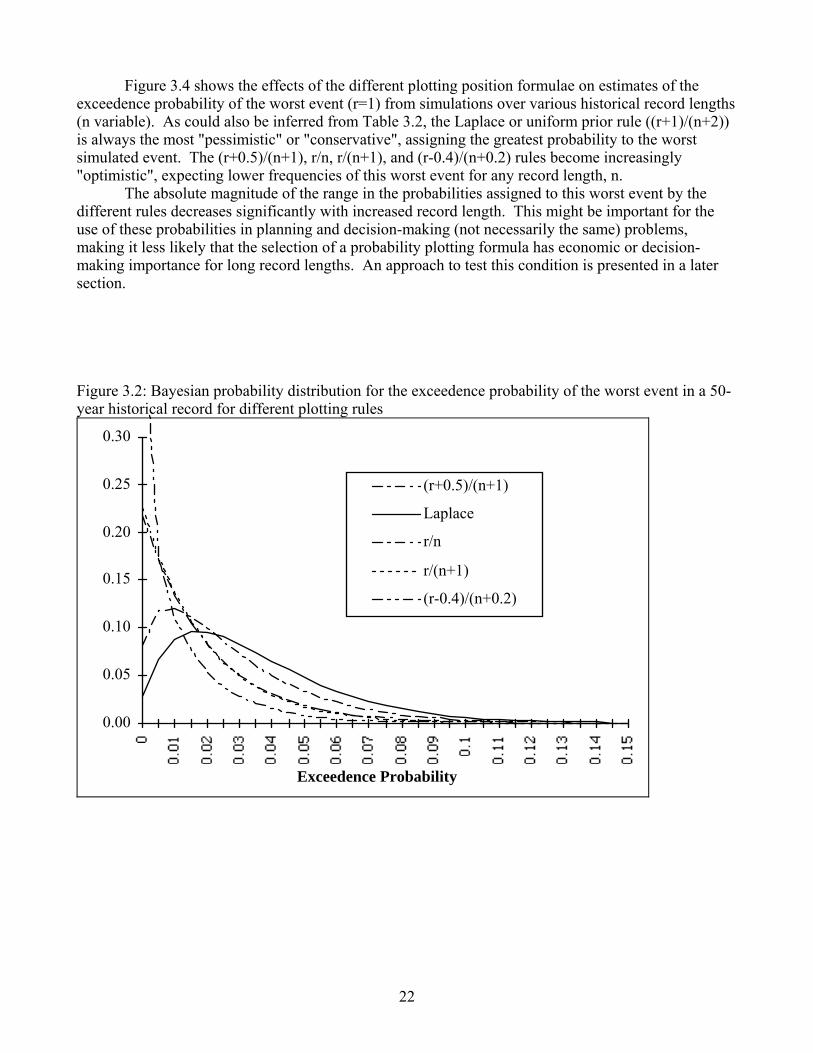
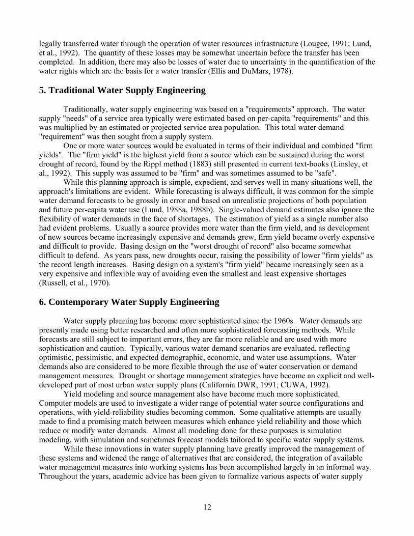
Figure 3.4 shows the effects of the different plotting position formulae on estimates of the exceedence probability of the worst event (r=1) from simulations over various historical record lengths (n variable). As could also be inferred from Table 3.2, the Laplace or uniform prior rule ((r+1)/(n+2)) is always the most "pessimistic" or "conservative", assigning the greatest probability to the worst simulated event. The (r+0.5)/(n+1), r/n, r/(n+1), and (r-0.4)/(n+0.2) rules become increasingly "optimistic", expecting lower frequencies of this worst event for any record length, n. The absolute magnitude of the range in the probabilities assigned to this worst event by the different rules decreases significantly with increased record length. This might be important for the use of these probabilities in planning and decision-making (not necessarily the same) problems, making it less likely that the selection of a probability plotting formula has economic or decision-making importance for long record lengths. An approach to test this condition is presented in a later section. Figure 3.2: Bayesian probability distribution for the exceedence probability of the worst event in a 50-year historical record for different plotting rules

0.00

0.05

0.10

0.15

0.20

0.25

0.30

Exceedence Probability

(r+0.5)/(n+1)

Laplace

r/n

r/(n+1)

(r-0.4)/(n+0.2)

22

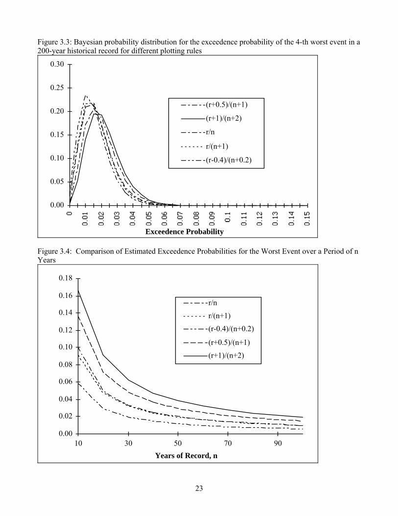
Figure 3.3: Bayesian probability distribution for the exceedence probability of the 4-th worst event in a 200-year historical record for different plotting rules

0.00

0.05

0.10

0.15

0.20

0.25

0.30

Exceedence Probability

(r+0.5)/(n+1)

(r+1)/(n+2)

r/n

r/(n+1)

(r-0.4)/(n+0.2)

Figure 3.4: Comparison of Estimated Exceedence Probabilities for the Worst Event over a Period of n Years

0.00

0.02

0.04

0.06

0.08

0.10

0.12

0.14

0.16

0.18

10 30 50 70 90Years of Record, n

r/n

r/(n+1)

(r-0.4)/(n+0.2)

(r+0.5)/(n+1)

(r+1)/(n+2)

23

7. Interpolating and Extrapolating with Rare Shortage Events Another problem posed in probabilistic planning for water supplies using historical hydrology is that there are rarely shortages that result from a repeat of the historical record. Most water supply systems have been designed using a firm yield approach, often implying that no shortage is expected with a repeat of the worst drought of record. Assigning probabilities to the range of unexperienced and unrepresented severe drought hydrologies requires extrapolation beyond the worst event of record.

The remaining cumulative probability, 1-P- worst, must be distributed over the range of shortages between the worst shortage simulated and 100% shortage, the un-exceedable maximum. A lesser, but still potentially important problem is distributing probability among shortage or yield levels that fall between shortage or yield events realized in the simulation results. Where shortage events are rare, numbering typically less than half a dozen in a record length of over 50 years, there is likely to be some coarseness to the realized events relative to what would be desirable for planning or decision-making purposes. If a simulation run with a 50-year historical hydrology yields only three shortages, one each of 10%, 40%, and 50%, what is the probability of a 20% or 30% shortage? This is an interesting, but hopefully unimportant, problem. A maximum-entropy (Tribus, 1969; Englehardt and Lund, 1992; Jaynes, 1996) approach to this problem would be to uniformly distribute the differences in cumulative distribution values between realized shortage or yield values, i.e., linear interpolation of probability between shortage result values. Thus, for the question above, the exceedence probability assigned to the 20% shortage level would be that of the 10% shortage level, plus one third of the difference between the exceedence probabilities of the 40% and 10% shortages (found by plotting positions). Still another approach would be to fit a cumulative distribution to those few points estimated by plotting positions formula, perhaps using a spline fit to preserve the plotting positions of the simulated results. This issue appears unresolved. 8. Limitations and Concerns Two major potential limitations and concerns arise in this analysis. First, is the Bernoulli distribution an appropriate likelihood function for use in this application of Bayes' theorem? The use of a Bernoulli likelihood function in Equation 5 brings the assumption that shortage events are not correlated in time. We know this is frequently not true. Yet, if shortage or yield events are correlated in time, what should be the likelihood function for use in Bayes' theorem? This problem is further compounded by the likely variability of the correlation of yields or shortages with different system configurations or operating policy decisions. Second, what is a proper basis for evaluating or selecting prior distributions for exceedence probabilities? A related concern is, shouldn't the prior probability distribution of exceedence probabilities vary with different shortage levels? The mean prior exceedence probability of a small shortage always should be greater than that of larger shortages. However, water supply reservoir systems can be operated such that small shortages occur less frequently than large shortages (Hashimoto, et al., 1981), changing the rate of change in exceedence probability with shortage level. Thus, it can be difficult to specify the proper prior distribution without knowing the operating policies of the reservoir system. Without a firmer basis for varying the prior with shortage level, prior distributions have not been varied here with shortage or yield level. The effect of not decreasing the expected value of the prior exceedence probability distribution with increasing shortage is to overestimate the posterior expected value of shortage exceedence probability for larger shortages. As

24

these two concerns demonstrate, there are many Bayesian approaches to examining the problem of plotting positions. 9. Does Plotting Position Formula Matter for Water Supply? For the example set of rather severe shortage results from a system yield model appearing in Table 3.3, exceedence probability distributions are generated for each of the foregoing plotting position formulae. A two-stage linear program for shortage management then was employed to evaluate the willingness to pay of customers to avoid each of the resulting shortage probability distributions (Lund, 1995). The shortage management options and costs used for the two-stage linear program are the same in all cases and are those used in the annual case of Chapter 4. The willingness-to-pay results of these two-stage linear programs appear in Table 3.4. This provides a general approach for determining the economic and decision-making importance of plotting position formulae for particular urban water supply problems. The results appearing in these tables indicate the sensitivity of shortage management decisions and their expected value costs to changes in plotting position formula. Expected value costs are measured by the expected value of the willingness-to-pay to avoid the shortage (Lund, 1995). As can be seen in Table 3.3, for this example there is little difference in the exceedence probability estimates between the r/n and r/(n+1) plotting rules. For other plotting rules, differences in exceedence probabilities are more wide-ranging. But are these differences in exceedence probability estimates important from a system management and engineering perspective? Table 3.4 shows the expected value of the service area's willingness to pay to avoid the shortages presented in Table 3.3. For this case, there are no differences in the long and short-term management decisions (various water conservation and water transfer arrangements) taken in response to these shortages, except for the Laplace ((r+1)/(n+2)) plotting formula. The differences in willingness to pay to avoid shortages for these first four plotting rules here arise solely from the different probabilities assigned to each shortage level for the expected value calculations. This difference in expected shortage costs estimated from the different plotting position formulae would seem to encourage greater hedging in storage operations where the more "pessimistic" of the first four plotting position formulae are used (such as (r+0.5)/(n+1)). In addition, changes in the plotting position rule also affect the overall probability of any shortage, which can affect both shortage management decisions and the expected value costs of any set of decisions. For this case, the greater shortage probabilities from the use of the Laplace plotting rule change least-cost shortage management decisions as well as further increase the expected value of shortage costs which result from these decisions. The changes in shortage management decisions include a shift from some short-term management measures (emergency water conservation and spot-market water transfers) to more long-term measures (plumbing retrofits and dry-year-option water transfers). For this moderately severe case, the selection of a shortage plotting position formula appears to have some importance for evaluating alternative system configuration and operation decisions (reflected in differences in the expected shortage cost values). The choice of plotting formula can also be important for the design of least-cost shortage management plans.

25

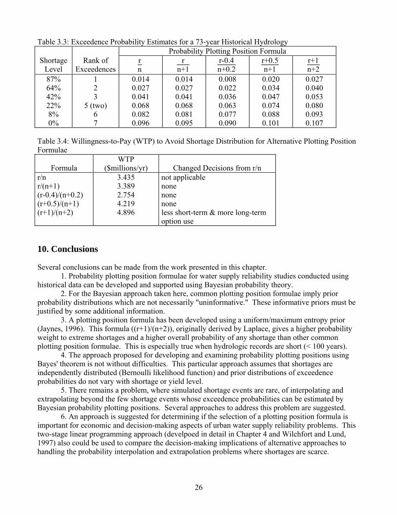
Table 3.3: Exceedence Probability Estimates for a 73-year Historical Hydrology Probability Plotting Position Formula

Shortage Level

Rank of Exceedences

rn

rn+1

r-0.4n+0.2

r+0.5n+1

r+1n+2

87% 1 0.014 0.014 0.008 0.020 0.027 64% 2 0.027 0.027 0.022 0.034 0.040 42% 3 0.041 0.041 0.036 0.047 0.053 22% 5 (two) 0.068 0.068 0.063 0.074 0.080 8% 6 0.082 0.081 0.077 0.088 0.093 0% 7 0.096 0.095 0.090 0.101 0.107

Table 3.4: Willingness-to-Pay (WTP) to Avoid Shortage Distribution for Alternative Plotting Position Formulae

Formula

WTP ($millions/yr)

Changed Decisions from r/n

r/n 3.435 not applicable r/(n+1) 3.389 none (r-0.4)/(n+0.2) 2.754 none (r+0.5)/(n+1) 4.219 none (r+1)/(n+2) 4.896 less short-term & more long-term

option use 10. Conclusions Several conclusions can be made from the work presented in this chapter. 1. Probability plotting position formulae for water supply reliability studies conducted using historical data can be developed and supported using Bayesian probability theory. 2. For the Bayesian approach taken here, common plotting position formulae imply prior probability distributions which are not necessarily "uninformative." These informative priors must be justified by some additional information. 3. A plotting position formula has been developed using a uniform/maximum entropy prior (Jaynes, 1996). This formula ((r+1)/(n+2)), originally derived by Laplace, gives a higher probability weight to extreme shortages and a higher overall probability of any shortage than other common plotting position formulae. This is especially true when hydrologic records are short (< 100 years). 4. The approach proposed for developing and examining probability plotting positions using Bayes' theorem is not without difficulties. This particular approach assumes that shortages are independently distributed (Bernoulli likelihood function) and prior distributions of exceedence probabilities do not vary with shortage or yield level. 5. There remains a problem, where simulated shortage events are rare, of interpolating and extrapolating beyond the few shortage events whose exceedence probabilities can be estimated by Bayesian probability plotting positions. Several approaches to address this problem are suggested. 6. An approach is suggested for determining if the selection of a plotting position formula is important for economic and decision-making aspects of urban water supply reliability problems. This two-stage linear programming approach (develpoed in detail in Chapter 4 and Wilchfort and Lund, 1997) also could be used to compare the decision-making implications of alternative approaches to handling the probability interpolation and extrapolation problems where shortages are scarce.

26

Chapter 4 Shortage Management Model

"It is recognized by all water professionals that the science of design and evaluation of water conservation programs has lagged behind the interest in, and need for, these programs." California Urban Water Agencies (1992) 1. Introduction This chapter describes the development and application of a shortage management model. This particular shortage management model employs available water shortage management measures to minimize average costs given hydrologic uncertainties (Wilchfort and Lund, 1997). The model is applied to a simplified EBMUD system and expanded to several examples which demonstrate the strengths of the model in incorporating the effects of seasonal shortages, water qualities, and uncertainties relating to the long term and short term management options. Water shortages and threats of water shortages have resulted in expanded consideration and development of demand management, supply enhancement, and water transfer measures. A wide range of available demand and supply management measures can be considered in devising a management plan to respond to shortage events. In developing shortage management practices, the effects of uncertainties associated with hydrology, water demands, environmental requirements and regulations, and availability of resources ideally should be examined. Other factors that can significantly affect management decisions are the effects of seasonal shortages, limitations on imported water during drought events, the effects of system operation, and the qualities of waters supplied and demanded. Several methods have been developed to integrate different demand management measures in water supply planning. These methods examined the use of conservation measures to delay the construction of new supply sources (Rubenstein and Ortolano, 1984; Lund, 1987), the trade-off between long term and short term conservation efforts (Dziegielewski, et al., 1992), and the incorporation of water transfers as an option to increase system reliability (Lund and Israel, 1995). This chapter describes the use of two-stage linear programming optimization to integrate long term and short term demand management and water transfer options for least-cost shortage management, considering yield reliability (Lund, 1995; Lund and Israel, 1995). The effects of hydrologic uncertainty, system operation, the availability of resources, water uses, costs, and available water supply qualities are incorporated into the model. 2. Optimization Models for Integrated Shortage Management Optimization models are mathematical representations of problems that suggest solutions based on predefined objectives. Optimization models have three main components. First, an objective function is required to measure system performance. Common objective functions are cost minimization, benefit maximization, yield maximization, or environmental quality preservation. Second, decision variables represent the available options (engineering or planning decisions) which can affect the objective. In this case decision variables might represent the amount and timing of specific water conservation or water transfer measures. Third, constraints are mathematical representations of the limitations on available decisions/decision variables. Constraints can be based on decision logistics, physical and operational constraints, and policy and environmental regulations. Several optimization models have been developed to assist in shortage planning and

27

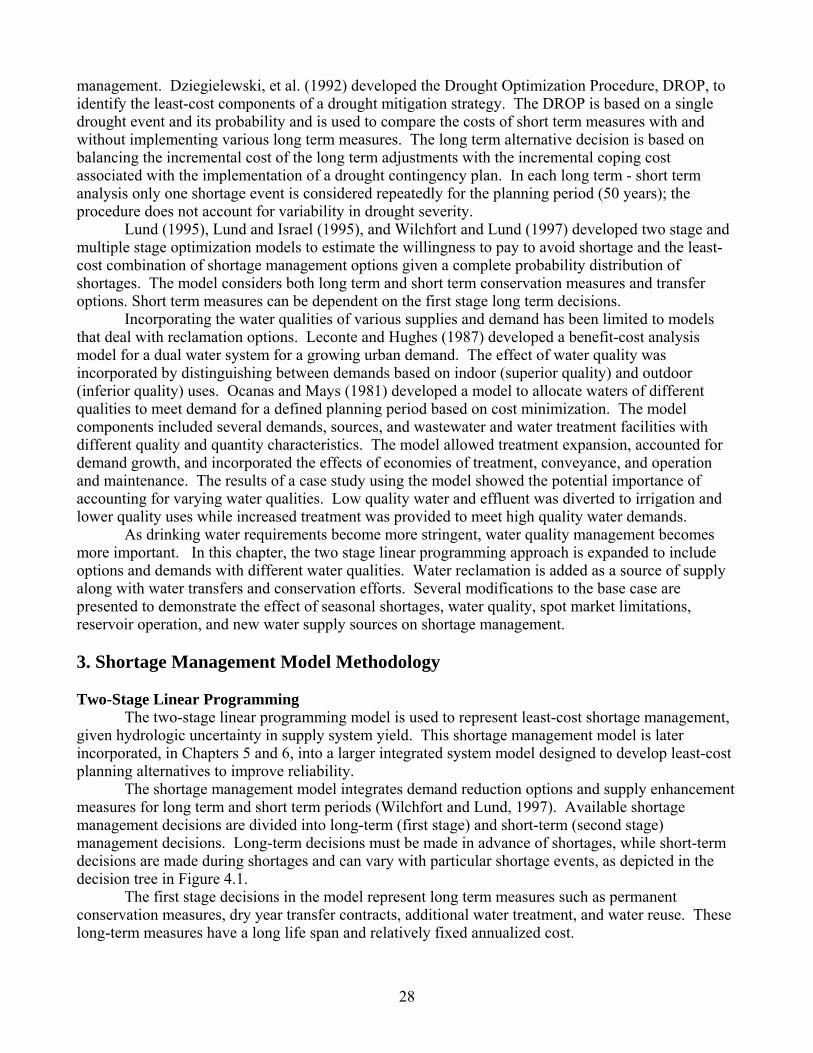
management. Dziegielewski, et al. (1992) developed the Drought Optimization Procedure, DROP, to identify the least-cost components of a drought mitigation strategy. The DROP is based on a single drought event and its probability and is used to compare the costs of short term measures with and without implementing various long term measures. The long term alternative decision is based on balancing the incremental cost of the long term adjustments with the incremental coping cost associated with the implementation of a drought contingency plan. In each long term - short term analysis only one shortage event is considered repeatedly for the planning period (50 years); the procedure does not account for variability in drought severity. Lund (1995), Lund and Israel (1995), and Wilchfort and Lund (1997) developed two stage and multiple stage optimization models to estimate the willingness to pay to avoid shortage and the least-cost combination of shortage management options given a complete probability distribution of shortages. The model considers both long term and short term conservation measures and transfer options. Short term measures can be dependent on the first stage long term decisions. Incorporating the water qualities of various supplies and demand has been limited to models that deal with reclamation options. Leconte and Hughes (1987) developed a benefit-cost analysis model for a dual water system for a growing urban demand. The effect of water quality was incorporated by distinguishing between demands based on indoor (superior quality) and outdoor (inferior quality) uses. Ocanas and Mays (1981) developed a model to allocate waters of different qualities to meet demand for a defined planning period based on cost minimization. The model components included several demands, sources, and wastewater and water treatment facilities with different quality and quantity characteristics. The model allowed treatment expansion, accounted for demand growth, and incorporated the effects of economies of treatment, conveyance, and operation and maintenance. The results of a case study using the model showed the potential importance of accounting for varying water qualities. Low quality water and effluent was diverted to irrigation and lower quality uses while increased treatment was provided to meet high quality water demands. As drinking water requirements become more stringent, water quality management becomes more important. In this chapter, the two stage linear programming approach is expanded to include options and demands with different water qualities. Water reclamation is added as a source of supply along with water transfers and conservation efforts. Several modifications to the base case are presented to demonstrate the effect of seasonal shortages, water quality, spot market limitations, reservoir operation, and new water supply sources on shortage management. 3. Shortage Management Model Methodology Two-Stage Linear Programming The two-stage linear programming model is used to represent least-cost shortage management, given hydrologic uncertainty in supply system yield. This shortage management model is later incorporated, in Chapters 5 and 6, into a larger integrated system model designed to develop least-cost planning alternatives to improve reliability. The shortage management model integrates demand reduction options and supply enhancement measures for long term and short term periods (Wilchfort and Lund, 1997). Available shortage management decisions are divided into long-term (first stage) and short-term (second stage) management decisions. Long-term decisions must be made in advance of shortages, while short-term decisions are made during shortages and can vary with particular shortage events, as depicted in the decision tree in Figure 4.1. The first stage decisions in the model represent long term measures such as permanent conservation measures, dry year transfer contracts, additional water treatment, and water reuse. These long-term measures have a long life span and relatively fixed annualized cost.

28

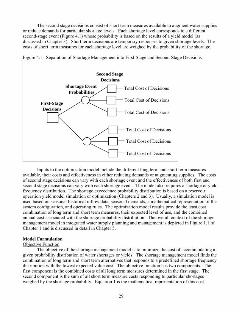
The second stage decisions consist of short term measures available to augment water supplies or reduce demands for particular shortage levels. Each shortage level corresponds to a different second-stage event (Figure 4.1) whose probability is based on the results of a yield model (as discussed in Chapter 3). Short term decisions are temporary responses to given shortage levels. The costs of short term measures for each shortage level are weighed by the probability of the shortage. Figure 4.1: Separation of Shortage Management into First-Stage and Second-Stage Decisions

First-Stage Decisions

Shortage Event Probabilities

Second Stage Decisions

Total Cost of Decisions

Total Cost of Decisions

Total Cost of Decisions

Total Cost of Decisions

Total Cost of Decisions

Total Cost of Decisions

Inputs to the optimization model include the different long term and short term measures available, their costs and effectiveness in either reducing demands or augmenting supplies. The costs of second stage decisions can vary with each shortage event and the effectiveness of both first and second stage decisions can vary with each shortage event. The model also requires a shortage or yield frequency distribution. The shortage exceedence probability distribution is based on a reservoir operation yield model simulation or optimization (Chapters 2 and 3). Usually, a simulation model is used based on seasonal historical inflow data, seasonal demands, a mathematical representation of the system configuration, and operating rules. The optimization model results provide the least cost combination of long term and short term measures, their expected level of use, and the combined annual cost associated with the shortage probability distribution. The overall context of the shortage management model in integrated water supply planning and management is depicted in Figure 1.1 of Chapter 1 and is discussed in detail in Chapter 5. Model Formulation Objective Function The objective of the shortage management model is to minimize the cost of accommodating a given probability distribution of water shortages or yields. The shortage management model finds the combination of long term and short term alternatives that responds to a predefined shortage frequency distribution with the lowest expected value cost. The objective function has two components. The first component is the combined costs of all long term measures determined in the first stage. The second component is the sum of all short term measure costs responding to particular shortages weighed by the shortage probability. Equation 1 is the mathematical representation of this cost

29

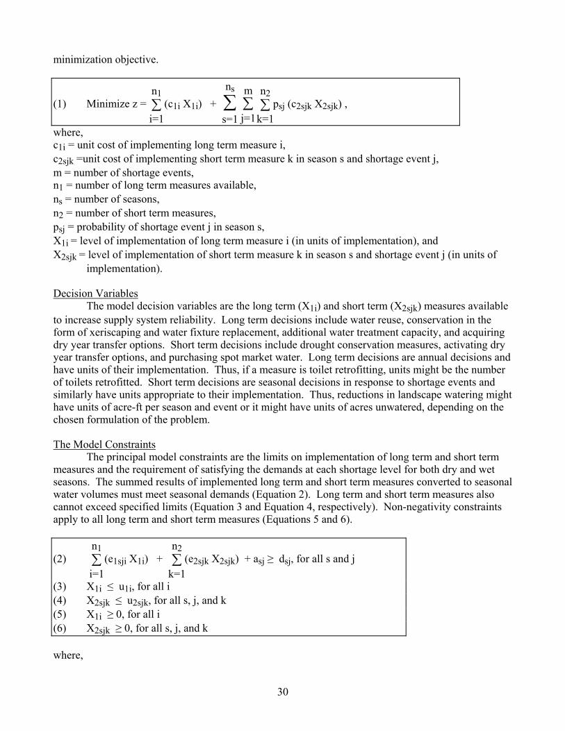
minimization objective.

(1) Minimize z = ∑i=1

n1 (c1i X1i) + ∑

s=1

ns

∑j=1

m ∑k=1

n2 psj (c2sjk X2sjk) ,

where, c1i = unit cost of implementing long term measure i, c2sjk =unit cost of implementing short term measure k in season s and shortage event j, m = number of shortage events, n1 = number of long term measures available, ns = number of seasons, n2 = number of short term measures, psj = probability of shortage event j in season s, X1i = level of implementation of long term measure i (in units of implementation), and X2sjk = level of implementation of short term measure k in season s and shortage event j (in units of

implementation). Decision Variables The model decision variables are the long term (X1i) and short term (X2sjk) measures available to increase supply system reliability. Long term decisions include water reuse, conservation in the form of xeriscaping and water fixture replacement, additional water treatment capacity, and acquiring dry year transfer options. Short term decisions include drought conservation measures, activating dry year transfer options, and purchasing spot market water. Long term decisions are annual decisions and have units of their implementation. Thus, if a measure is toilet retrofitting, units might be the number of toilets retrofitted. Short term decisions are seasonal decisions in response to shortage events and similarly have units appropriate to their implementation. Thus, reductions in landscape watering might have units of acre-ft per season and event or it might have units of acres unwatered, depending on the chosen formulation of the problem. The Model Constraints The principal model constraints are the limits on implementation of long term and short term measures and the requirement of satisfying the demands at each shortage level for both dry and wet seasons. The summed results of implemented long term and short term measures converted to seasonal water volumes must meet seasonal demands (Equation 2). Long term and short term measures also cannot exceed specified limits (Equation 3 and Equation 4, respectively). Non-negativity constraints apply to all long term and short term measures (Equations 5 and 6).

(2) ∑i=1

n1 (e1sji X1i) + ∑

k=1

n2 (e2sjk X2sjk) + asj ≥ dsj, for all s and j

(3) X1i ≤ u1i, for all i (4) X2sjk ≤ u2sjk, for all s, j, and k (5) X1i ≥ 0, for all i (6) X2sjk ≥ 0, for all s, j, and k where,

30

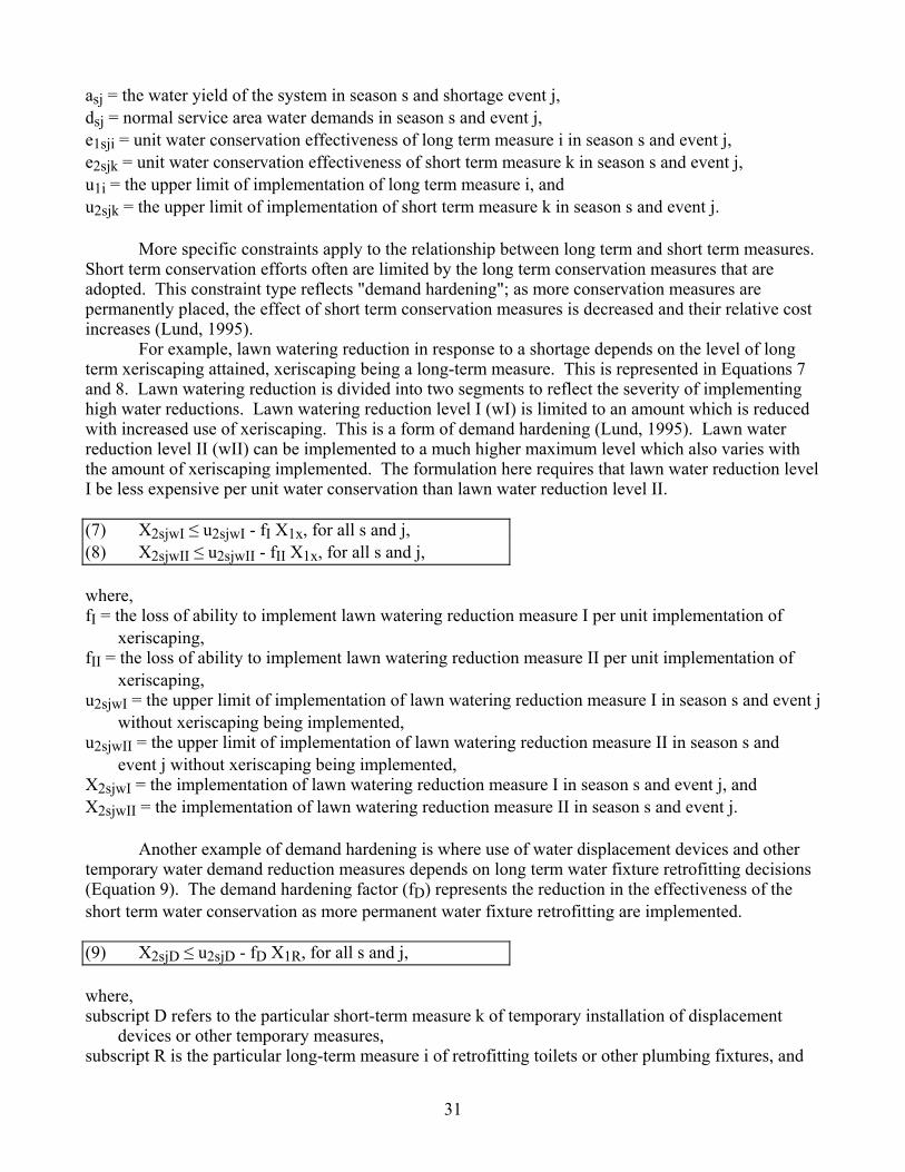
asj = the water yield of the system in season s and shortage event j, dsj = normal service area water demands in season s and event j, e1sji = unit water conservation effectiveness of long term measure i in season s and event j, e2sjk = unit water conservation effectiveness of short term measure k in season s and event j, u1i = the upper limit of implementation of long term measure i, and u2sjk = the upper limit of implementation of short term measure k in season s and event j. More specific constraints apply to the relationship between long term and short term measures. Short term conservation efforts often are limited by the long term conservation measures that are adopted. This constraint type reflects "demand hardening"; as more conservation measures are permanently placed, the effect of short term conservation measures is decreased and their relative cost increases (Lund, 1995). For example, lawn watering reduction in response to a shortage depends on the level of long term xeriscaping attained, xeriscaping being a long-term measure. This is represented in Equations 7 and 8. Lawn watering reduction is divided into two segments to reflect the severity of implementing high water reductions. Lawn watering reduction level I (wI) is limited to an amount which is reduced with increased use of xeriscaping. This is a form of demand hardening (Lund, 1995). Lawn water reduction level II (wII) can be implemented to a much higher maximum level which also varies with the amount of xeriscaping implemented. The formulation here requires that lawn water reduction level I be less expensive per unit water conservation than lawn water reduction level II. (7) X2sjwI ≤ u2sjwI - fI X1x, for all s and j, (8) X2sjwII ≤ u2sjwII - fII X1x, for all s and j, where, fI = the loss of ability to implement lawn watering reduction measure I per unit implementation of

xeriscaping, fII = the loss of ability to implement lawn watering reduction measure II per unit implementation of

xeriscaping, u2sjwI = the upper limit of implementation of lawn watering reduction measure I in season s and event j

without xeriscaping being implemented, u2sjwII = the upper limit of implementation of lawn watering reduction measure II in season s and

event j without xeriscaping being implemented, X2sjwI = the implementation of lawn watering reduction measure I in season s and event j, and X2sjwII = the implementation of lawn watering reduction measure II in season s and event j. Another example of demand hardening is where use of water displacement devices and other temporary water demand reduction measures depends on long term water fixture retrofitting decisions (Equation 9). The demand hardening factor (fD) represents the reduction in the effectiveness of the short term water conservation as more permanent water fixture retrofitting are implemented. (9) X2sjD ≤ u2sjD - fD X1R, for all s and j, where, subscript D refers to the particular short-term measure k of temporary installation of displacement

devices or other temporary measures, subscript R is the particular long-term measure i of retrofitting toilets or other plumbing fixtures, and

31

fD = the unit reduction of displacement device effectiveness with implementation of plumbing retrofitting.

Water transfers often are limited by the treatment capacity available to accommodate lower quality transferred water. As a long-term measure, water treatment capacity can be expanded to increase the quantity of water that can be contracted as dry year option or purchased from spot markets (Equation 10). For each shortage level, the amount of dry year option activated is dependent on the long term decision of the dry year option contract (Equation 11). The sum of spot market purchases and activated dry year options must not exceed the total transfer limit which might vary with shortage event (Equation 12). (10) TTs ≤ CAPs + ws X1c, for all s (11) X2sjO ≤ X1Os, for all s, j, and option measures O

(12) ∑l=1

nT (X2sjl) ≤ TTs, for all s and j

where, CAPs = existing water treatment capacity, in volumetric units for season s, nT = the number of short-term and long term transfer decisions available, TTs = total transfers in season s, X1c = the additions to water treatment capacity (typically in mgd), and ws = the seasonal volume of additional water treatment capability per unit increase in treatment plant

capacity for season s. 4. Base Case Example The East Bay Municipal Utility District The East Bay Municipal Utility District (EBMUD) system is used to illustrate the use of the shortage management model in developing an integrated resources planning scheme. The EBMUD system serves over one million people in Alameda and Contra Costa counties. Most of the water serving these counties is supplied from the Mokelumne River. The Pardee and Camanche reservoirs, along with local storage reservoirs in the service area, serve the EBMUD with a combined capacity of about 720 thousand acre-ft (TAF). Future EBMUD service area water demands in 2020 are expected to total 280 TAF/year. The ability to meet future demand may become limited due to decreasing availability of water supply sources as a result of increased consumption by senior water rights holders, increasing instream requirements to protect fish, wildlife, and riparian habitat, and limited new water sources. The ability to supply adequate water also is limited due to increasingly stringent water quality standards. Both the availability of water and the quality of sources are therefore important for future water allocation. Water yields and shortages for the EBMUD service area were estimated using a simplified yield simulation model presented in Chapter 6. Probabilities were assigned to these results using the procedures described in Chapter 3. Incorporating Shortage Management Options For this study, management options were somewhat simplified from what they should be for an actual study of a system of this size. Long term measures considered in the model are conservation, dry year option transfers, water treatment capacity expansion, and water reuse. Long term

32

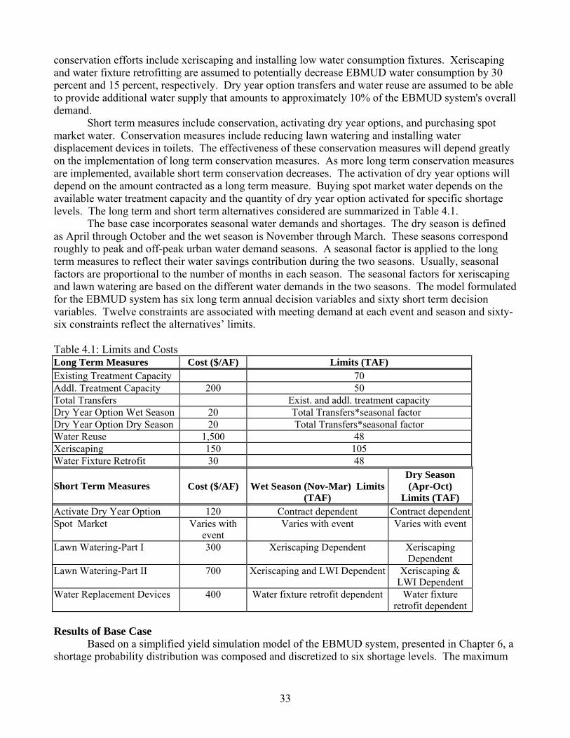
conservation efforts include xeriscaping and installing low water consumption fixtures. Xeriscaping and water fixture retrofitting are assumed to potentially decrease EBMUD water consumption by 30 percent and 15 percent, respectively. Dry year option transfers and water reuse are assumed to be able to provide additional water supply that amounts to approximately 10% of the EBMUD system's overall demand. Short term measures include conservation, activating dry year options, and purchasing spot market water. Conservation measures include reducing lawn watering and installing water displacement devices in toilets. The effectiveness of these conservation measures will depend greatly on the implementation of long term conservation measures. As more long term conservation measures are implemented, available short term conservation decreases. The activation of dry year options will depend on the amount contracted as a long term measure. Buying spot market water depends on the available water treatment capacity and the quantity of dry year option activated for specific shortage levels. The long term and short term alternatives considered are summarized in Table 4.1. The base case incorporates seasonal water demands and shortages. The dry season is defined as April through October and the wet season is November through March. These seasons correspond roughly to peak and off-peak urban water demand seasons. A seasonal factor is applied to the long term measures to reflect their water savings contribution during the two seasons. Usually, seasonal factors are proportional to the number of months in each season. The seasonal factors for xeriscaping and lawn watering are based on the different water demands in the two seasons. The model formulated for the EBMUD system has six long term annual decision variables and sixty short term decision variables. Twelve constraints are associated with meeting demand at each event and season and sixty-six constraints reflect the alternatives’ limits. Table 4.1: Limits and Costs Long Term Measures Cost ($/AF) Limits (TAF) Existing Treatment Capacity 70 Addl. Treatment Capacity 200 50 Total Transfers Exist. and addl. treatment capacity Dry Year Option Wet Season 20 Total Transfers*seasonal factor Dry Year Option Dry Season 20 Total Transfers*seasonal factor Water Reuse 1,500 48 Xeriscaping 150 105 Water Fixture Retrofit 30 48 Short Term Measures

Cost ($/AF)

Wet Season (Nov-Mar) Limits

(TAF)

Dry Season (Apr-Oct)

Limits (TAF) Activate Dry Year Option 120 Contract dependent Contract dependentSpot Market Varies with

event Varies with event Varies with event

Lawn Watering-Part I 300

Xeriscaping Dependent Xeriscaping Dependent

Lawn Watering-Part II 700

Xeriscaping and LWI Dependent Xeriscaping & LWI Dependent

Water Replacement Devices 400

Water fixture retrofit dependent Water fixture retrofit dependent

Results of Base Case Based on a simplified yield simulation model of the EBMUD system, presented in Chapter 6, a shortage probability distribution was composed and discretized to six shortage levels. The maximum

33

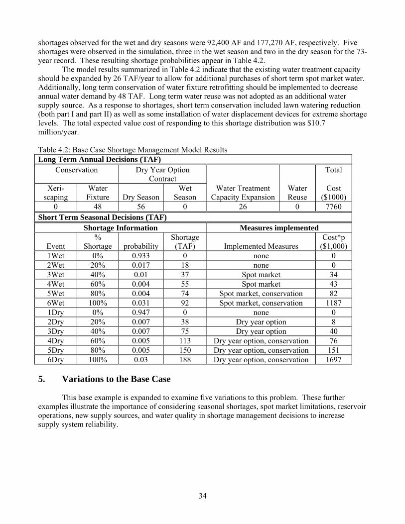
shortages observed for the wet and dry seasons were 92,400 AF and 177,270 AF, respectively. Five shortages were observed in the simulation, three in the wet season and two in the dry season for the 73-year record. These resulting shortage probabilities appear in Table 4.2. The model results summarized in Table 4.2 indicate that the existing water treatment capacity should be expanded by 26 TAF/year to allow for additional purchases of short term spot market water. Additionally, long term conservation of water fixture retrofitting should be implemented to decrease annual water demand by 48 TAF. Long term water reuse was not adopted as an additional water supply source. As a response to shortages, short term conservation included lawn watering reduction (both part I and part II) as well as some installation of water displacement devices for extreme shortage levels. The total expected value cost of responding to this shortage distribution was $10.7 million/year. Table 4.2: Base Case Shortage Management Model Results Long Term Annual Decisions (TAF)

Conservation Dry Year Option Contract

Total

Xeri-scaping

Water Fixture

Dry Season

Wet Season

Water Treatment Capacity Expansion

Water Reuse

Cost ($1000)

0 48 56 0 26 0 7760 Short Term Seasonal Decisions (TAF)

Shortage Information Measures implemented

Event %

Shortage

probability Shortage

(TAF)

Implemented Measures Cost*p

($1,000) 1Wet 0% 0.933 0 none 0 2Wet 20% 0.017 18 none 0 3Wet 40% 0.01 37 Spot market 34 4Wet 60% 0.004 55 Spot market 43 5Wet 80% 0.004 74 Spot market, conservation 82 6Wet 100% 0.031 92 Spot market, conservation 1187 1Dry 0% 0.947 0 none 0 2Dry 20% 0.007 38 Dry year option 8 3Dry 40% 0.007 75 Dry year option 40 4Dry 60% 0.005 113 Dry year option, conservation 76 5Dry 80% 0.005 150 Dry year option, conservation 151 6Dry 100% 0.03 188 Dry year option, conservation 1697

5. Variations to the Base Case This base example is expanded to examine five variations to this problem. These further examples illustrate the importance of considering seasonal shortages, spot market limitations, reservoir operations, new supply sources, and water quality in shortage management decisions to increase supply system reliability.

34

Seasonal vs. Annual Models Annual and seasonal yield simulation models can produce significantly different shortage probability distributions. The difference in the distributions can be attributed to the rough averaging and lumping of the annual simulation model. An annual system model will tend to experience less severe shortages and will tend to recover faster than a seasonal simulation model. The differences between annual and seasonal time step simulation models are reflected in Figure 4.2, indicating the difference in the extent of storage depletion and the length of time required for the system to recover under both scenarios. Depletion of storage is more severe for the seasonal model simulation as shown in year 15 and may take longer to recover as shown in years 27 through 31. Figure 4.2: Comparison of End-of-year Storages for Annual and Seasonal Yield Models

0

100,000

200,000

300,000

400,000

500,000

600,000

700,000

800,000

1 5 9 13 17 21 25 29 33 37 41 45 49 53 57 61 65 69 73

Year

Annual ModelSeasonal Model

The difference in the probability distribution can affect the results of the shortage management optimization model. A comparison of an annual model and a seasonal model indicates the different decisions and consequences of ignoring the effect of seasonality. Shortage magnitudes and frequencies for the annual and seasonal models are summarized in Table 4.3. The average shortage based on the annual model was 9,744 AF while the average annual shortage based on the seasonal model is 11,795 AF (combined seasons). The seasonal model results included a 100% shortage absent in the annual model results. The difference in shortage probability distributions results in a significantly lower expected value cost of managing shortage, $3.2 million/year for the annual model versus $11.1 million/year for the seasonal model. More significant is the difference in management and planning decisions for the two types of simulation model. Due to the high probabilities of extreme shortages in the seasonal model, long term conservation is installed and water treatment capacity is enhanced. Spot market purchases and additional temporary conservation measures are implemented as necessary during particular shortage levels. Results of the shortage management model based on annual time steps are summarized in Table 4.4. The shortage management model results indicate that contracting dry year options is more cost efficient than spot market purchases since extreme shortages have low probabilities. Limited

35

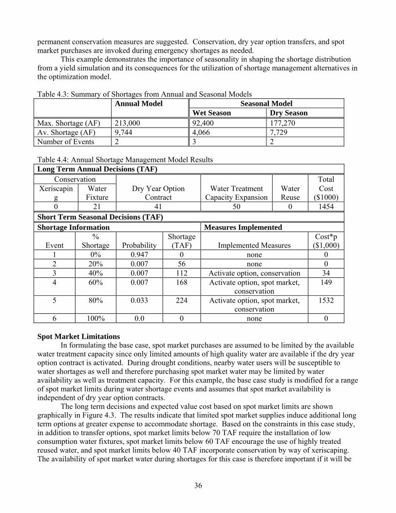
permanent conservation measures are suggested. Conservation, dry year option transfers, and spot market purchases are invoked during emergency shortages as needed. This example demonstrates the importance of seasonality in shaping the shortage distribution from a yield simulation and its consequences for the utilization of shortage management alternatives in the optimization model. Table 4.3: Summary of Shortages from Annual and Seasonal Models Annual Model Seasonal Model Wet Season Dry Season Max. Shortage (AF) 213,000 92,400 177,270 Av. Shortage (AF) 9,744 4,066 7,729 Number of Events 2 3 2 Table 4.4: Annual Shortage Management Model Results Long Term Annual Decisions (TAF)

Conservation Total Xeriscapin

g Water Fixture

Dry Year Option Contract

Water Treatment Capacity Expansion

Water Reuse

Cost ($1000)

0 21 41 50 0 1454 Short Term Seasonal Decisions (TAF) Shortage Information Measures Implemented

Event

% Shortage

Probability

Shortage (TAF)

Implemented Measures

Cost*p ($1,000)

1 0% 0.947 0 none 0 2 20% 0.007 56 none 0 3 40% 0.007 112 Activate option, conservation 34 4 60% 0.007 168 Activate option, spot market,

conservation 149

5 80% 0.033 224 Activate option, spot market, conservation

1532

6 100% 0.0 0 none 0 Spot Market Limitations In formulating the base case, spot market purchases are assumed to be limited by the available water treatment capacity since only limited amounts of high quality water are available if the dry year option contract is activated. During drought conditions, nearby water users will be susceptible to water shortages as well and therefore purchasing spot market water may be limited by water availability as well as treatment capacity. For this example, the base case study is modified for a range of spot market limits during water shortage events and assumes that spot market availability is independent of dry year option contracts. The long term decisions and expected value cost based on spot market limits are shown graphically in Figure 4.3. The results indicate that limited spot market supplies induce additional long term options at greater expense to accommodate shortage. Based on the constraints in this case study, in addition to transfer options, spot market limits below 70 TAF require the installation of low consumption water fixtures, spot market limits below 60 TAF encourage the use of highly treated reused water, and spot market limits below 40 TAF incorporate conservation by way of xeriscaping. The availability of spot market water during shortages for this case is therefore important if it will be

36

limited to less than 70 TAF, since the costs increase substantially. This example shows that availability of spot market water can be an important factor in shortage management. As the probability of obtaining spot market water during shortages decreases, more long term measures must be implemented.

Figure 4.3: Effects of Spot Market Limitations

0

10,000

20,000

30,000

40,000

50,000

60,000

70,000

80,000

90,000

20 30 40 50 60 70 80 90Spot market limits, TAF

0

20

40

60

80

100

120

Lon

g T

erm

Mea

sure

s, T

AF

EVcostTransfer OptionWater Fixture conservationWater ReuseXeriscaping conservation

Reservoir Operations with Hedging and Carryover Storage The probability distribution of shortages is affected largely by the capabilities and operation of the water supply's sources and reservoirs. Managers may prefer several smaller shortages to a few very large ones, since shortage costs typically increase disproportionately to shortage magnitudes. Modifying reservoir operating rules can often reduce overall damages associated with water shortages and improve reliability (Shih and ReVelle, 1995; Hirsch, 1987; Palmer and Holmes, 1988; Randall et al., 1990). Changing system operation alters the probability distribution of shortage events and may result in different shortage management decisions. Instituting carryover storage targets or hedging rules can induce small frequent shortages and reduce the frequency and magnitude of large shortages. This example demonstrates the effects of different levels of hedging and carryover storage on the probability distribution of shortage, least-cost shortage management, and the expected value of shortage management costs. The varying end of year storage as a result of different dry season hedging rules are shown in Figure 4.4, where the different curves represent operations at different levels of storage plus inflow at which hedging (releasing water less than total demand) is begun. The expected value costs based on different hedging rules during the wet and dry seasons are summarized in Table 4.5 and the effects of combined hedging rule and carry over storage are summarized in Table 4.6.

37

Figure 4.4: End of year storages for different hedging trigger rules

0

100,000

200,000

300,000

400,000

500,000

600,000

700,000

800,000

1 6 11 16 21 26 31 36 41 46 51 56 61 66 71 76

Year of Record

071254106881142508178135

Table 4.5: Hedging Rules Scenarios

Wet Season % Hedging 0% 10% 30% 50% 70% TAF Hedging

0 14.5 43.4 72.3 101.3

Cost ($1000) 11,077 11,182 11,207 9,080 9,113 Dry Season

% Hedging 0% 10% 20% 30% 40% 50% TAF Hedging

0 35.6 71.2 106.9 142.5 178.1

Cost ($1000) 11,077 11,142 10,476 10,483 10,753 11,008 Table 4.6: Carryover Scenarios with 72.3 TAF Wet Season Hedging Carryover Storage (TAF) 0 24.8 49.6 74.3 99.1 Cost ($1000) 9,080 9,083 8,936 8,308 8,246 Hedging in the dry season has a different effect on the system than hedging during the wet season. For this case, hedging in the wet season does not change end of year storage levels significantly or the frequency of shortages but decreases the maximum shortage event in the dry season. Hedging in the wet season induces more frequent shortages in the wet season and reduces the maximum shortage in the dry season. Because shortages in the dry season are more severe, wet season hedging has greater effect on the expected value cost of system reliability than dry season hedging. Incorporating carryover storage rules when storage levels become less than 200 TAF further reduces the overall shortage management cost. Using the different distributions to generate management plans results in the same long term decisions. The difference in overall shortage management cost results from the different extreme event probabilities and the magnitude of the short term measures used. The

38

effects of the various operating rules on shortage frequencies and magnitudes are summarized in Table 4.7. This example demonstrates the importance of reservoir operations in affecting the supply yield probability and in the planning decisions and costs of demand management and transfers. Depending on other costs associated with altering reservoir operations, it may be cost-effective to change operating rules and decrease the dependency on short term measures to improve supply system reliability. Table 4.7: The effect of operating rules on drought frequency and magnitude

Operating Rules

Base Case

Dry Season Hedging

(71.2 TAF)

Wet Season Hedging

(28.9 TAF)

Wet Season Hedging

with Carryover Storage (111.5 TAF)

Wet Season 0% shortage 0.933 0.947 0.933 0.933 20% shortage 0.017 0.017 0.004 0.004 40% shortage 0.01 0.006 0.004 0.004 60% shortage 0.004 0.031 0.004 0.004 80% shortage 0.004 0 0.015 0.013 100% shortage 0.031 0 0.039 0.04 Max. Shortage 92,400 50,085 92,400 92,400 Ave. Shortage 4,066 2,255 5,156 5,100 No. of Shortages 3 2 3 3 Dry Season 0% shortage 0.947 0.907 0.947 0.947 20% shortage 0.007 0.029 0.008 0.008 40% shortage 0.007 0.016 0.007 0.018 60% shortage 0.005 0.007 0.006 0.027 80% shortage 0.005 0.007 0.032 0 100% shortage 0.03 0.034 0 0 Max. Shortage 177,270 187,600 148,537 75,870 Ave. Shortage 7,729 10,506 6,303 4,690 No of Shortages 2 5 2 2 Overall cost ($1,000)

11,077 10,476 9,080 8,185

Several Water Qualities The base case assumes a single distribution system and the use of high quality water for all uses. This example is expanded to incorporate two water qualities: low quality and high quality. The low quality water demand is for selected landscaping and golf course water uses. Low quality water demands vary greatly between dry and wet seasons and are greatly affected by weather conditions and droughts. Use of low quality water is limited by the extent of a separate low-quality distribution system (usually part of a dual system). Having a separate distribution system allows the use of water of low quality from sources such as reused water, dry year options, and spot market purchases. Low quality water demands also can be reduced with conservation efforts such as xeriscaping and lawn watering reduction. High quality water also can be used for low quality uses. High quality water demand is a function of residential, commercial, and industrial uses. High

39

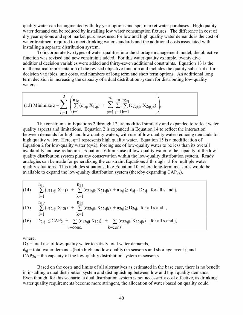
quality water can be augmented with dry year options and spot market water purchases. High quality water demand can be reduced by installing low water consumption fixtures. The difference in cost of dry year options and spot market purchases used for low and high quality water demands is the cost of water treatment required to meet drinking water standards and the additional costs associated with installing a separate distribution system. To incorporate two types of water qualities into the shortage management model, the objective function was revised and new constraints added. For this water quality example, twenty-five additional decision variables were added and thirty-seven additional constraints. Equation 13 is the mathematical representation of the revised objective function and includes the quality subscript q for decision variables, unit costs, and numbers of long term and short term options. An additional long term decision is increasing the capacity of a dual distribution system for distributing low-quality waters.

(13) Minimize z = ∑q=1

2

⎝⎜⎛

⎠⎟⎞

∑i=1

n1q (c1qi X1qi) + ∑

s=1

ns

∑j=1

m ∑k=1

n2q (c2qsjk X2qsjk) ,

The constraints in Equations 2 through 12 are modified similarly and expanded to reflect water quality aspects and limitations. Equation 2 is expanded in Equation 14 to reflect the interaction between demands for high and low quality waters, with use of low quality water reducing demands for high quality water. Here, q=1 represents high quality water. Equation 15 is a modification of Equation 2 for low-quality water (q=2), forcing use of low-quality water to be less than its overall availability and use-reduction. Equation 16 limits use of low-quality water to the capacity of the low-quality distribution system plus any conservation within the low-quality distribution system. Ready analogies can be made for generalizing the constraint Equations 3 through 13 for multiple water quality situations. This includes situations, like Equation 10, where long-term measures would be available to expand the low-quality distribution system (thereby expanding CAP2s).

(14) ∑i=1

n11 (e11sji X11i) + ∑

k=1

n21 (e21sjk X21sjk) + a1sj ≥ dsj - D2sj, for all s and j,

(15) ∑i=1

n12 (e12sji X12i) + ∑

k=1

n22 (e22sjk X22sjk) + a2sj ≥ D2sj, for all s and j,

(16) D2sj ≤ CAP2s + ∑i=cons.

(e12sji X12i) + ∑k=cons.

(e22sjk X22sjk) , for all s and j,

where, D2 = total use of low-quality water to satisfy total water demands, dsj = total water demands (both high and low quality) in season s and shortage event j, and CAP2s = the capacity of the low-quality distribution system in season s Based on the costs and limits of all alternatives as estimated in the base case, there is no benefit in installing a dual distribution system and distinguishing between low and high quality demands. Even though, for this scenario, a dual distribution system is not necessarily cost effective, as drinking water quality requirements become more stringent, the allocation of water based on quality could

40

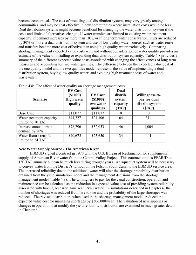
become economical. The cost of installing dual distribution systems may vary greatly among communities, and may be cost effective in new communities where installation costs would be less. Dual distribution systems might become beneficial for managing the water distribution system if the costs and limits of alternatives change. If water transfers are limited to existing water treatment capacity, if demand increases by more than 10%, or if long term water conservation limits are reduced by 30% or more, a dual distribution system and use of low quality water sources such as water reuse and transfers become more cost effective than using high quality water exclusively. Comparing shortage management expected value costs with and without consideration of water quality provides an estimate of the value of installing or expanding dual distribution system capacity. Table 4.8 provides a summary of the different expected value costs associated with changing the effectiveness of long term measures and accounting for two water qualities. The difference between the expected value cost of the one quality model and the two qualities model represents the value of implementing a dual distribution system, buying low quality water, and avoiding high treatment costs of water and wastewater. Table 4.8: The effect of water quality on shortage management costs

Scenario

EV Cost ($1000)

High water quality

EV Cost ($1000)

two water qualities

Dual distrib. system

capacity (TAF)

Willingness-to-

pay for dual distrib. system

($/AF) Base Case $11,077 $11,077 0 0 Water treatment capacity limited to 70 TAF

$44,227 $24,106

64 314

Increase annual urban demand by 20%

$78,296 $32,053 46 1,004

Water fixture retrofit limited to 24 TAF

$40,675 $25,650 34 441

New Water Supply Source - The American River EBMUD signed a contract in 1970 with the U.S. Bureau of Reclamation for supplemental supply of American River water from the Central Valley Project. This contract entitles EBMUD to 150 TAF annually but can be much less during drought years. An aqueduct system will be necessary to convey water from the District’s turnout on the Folsom South Canal to the EBMUD service area. The increased reliability due to the additional water will alter the shortage probability distribution obtained from the yield simulation model and the management decisions from the shortage management model (Table 4.9). The willingness to pay for the canal construction, operation and maintenance can be calculated as the reduction in expected value cost of providing system reliability associated with having access to American River water. In simulations described in Chapter 6, the number of shortages was reduced from five to two and the probability of the large shortages was reduced. The revised distribution, when used in the shortage management model, reduced the expected value cost for managing shortages by $306,000/year. The valuation of new supplies or changes in operation that modify the yield reliability distribution are examined in much greater detail in Chapter 6.

41

Table 4.9: Results of Shortage Management Model with American River Water Supply Long Term Annual Decisions (TAF)

Conservation Dry Year Option Contract

Total

Xeri-scaping

Water Fixture

Dry Season

Wet Season

Water Treatment Capacity Expansion

Water Reuse

Cost ($1000)

0 48 56 0 26 0 7,760 Short Term Seasonal Decisions (TAF)

Shortage Information Measures implemented

Event %

Shortage prob-ability

Shortage (TAF)

Measures Implemented

Cost*p

1Wet 0% 0.96 0 none 0 2Wet 20% 0.003 18 none 0 3Wet 40% 0.003 37 Spot market 10 4Wet 60% 0.003 55 Spot market 32 5Wet 80% 0.003 74 Spot market, conservation 62 6Wet 100% 0.029 92 Spot market, conservation 1,110 1Dry 0% 0.96 0 none 0 2Dry 20% 0.003 38 Dry year option 3 3Dry 40% 0.003 75 Dry year option 17 4Dry 60% 0.003 113 Dry year option, conservation 46 5Dry 80% 0.003 150 Dry year option, conservation 91 6Dry 100% 0.029 188 Dry year option, conservation 1,640

Total Expected Value Cost ($1,000): 10,771 6. Sensitivity Analysis Varying degrees of uncertainty are associated with determining the costs, limits, and effectiveness of the long term and short term measures used in the shortage management model. And these uncertainties depend on the water system studied. For example, the cost of water reuse which includes treatment cost, conveyance, and the benefit associated with utilizing wastewater effluent instead of discharging to the environment will vary with available technology, existing infrastructure, and changing environmental regulations. Both the quantity of water that can be saved through xeriscaping and the water that can be obtained through water transfers also are uncertain. Sensitivity analysis can be used to assess the potential effects of uncertainties on management decisions, the acceptable limits of errors and uncertainty, and the need to understand and quantify those uncertainties important to particular decision variables. Four types of sensitivity analysis can be gained readily from the two-stage linear programming approach presented here: Lagrange multipliers, slack variables, reduced cost, and range in unchanged basis. A further approach to sensitivity analysis is to merely re-solve the model for any combined cost, hydrologic, and technological scenario of particular concern. Since the model presented has a significant number of variables and constraints, the sensitivity analysis can help identify parameters that appear to be important and are prone to errors and a large degree of uncertainty. Lagrange Multipliers Lagrange multipliers (sometimes called dual values or shadow prices) represent the change in the objective function associated with a unit change in a constraint and are a by-product of linear

42

programming solution methods. For the model presented, the Lagrange multipliers represent the change in the overall expected value cost associated with changes in the long term and short term measure limits, water demand, shortage or yield amounts, or any other additive constant appearing in a single constraint. For the base case, the expected value cost is particularly sensitive to the availability of long term conservation water fixture retrofitting. Reducing demand by 1 acre-ft through conservation reduces the expected value cost by $131/year. The existing water treatment capacity is also an important factor in the overall expected value cost. Each additional acre-ft of available capacity reduces the expected value cost by $340/year. Slack Variables These values are the amount of unused long term and short term alternatives. Slack variables represent the amount that a constraint can be reduced before it will affect the objective function and the solution. High use of long term measures can create excess supply for what would otherwise be small shortage events. This will result in slack demand constraints for these small shortage events, encouraging the use of hedging in reservoir operations. Reduced Cost The reduced cost is the decrease in unit cost of a long or short term option needed before the option would be implemented by the cost minimizing model. Reduced costs are particularly important when exact costs and benefits associated with an option are not known with certainty. For the base case, long term xeriscaping conservation would be implemented if its cost is reduced from $150/AF to $20/AF, in which case it would be more cost effective than short term conservation reductions in lawn watering. Water reuse would be considered as an additional source of water if its unit cost is reduced to $225/AF in which case it would be more cost effective than implementing water transfers and the required additional water treatment capacity. Range in Unchanged Basis The allowable increase or decrease in the coefficients of both the objective function and the constraints is the range in which the same long term and short term decisions are preferred. Increasing the cost of the dry year option contract by $4/AF or more for the dry season will trigger more spot market purchases to replace the dry year alternative. On the other hand, reducing the cost of a dry year option contract by $3/AF will prompt use of the wet season contract option. For the base case, knowing the cost of contracting dry year option is important in developing long term and short term planning decisions. The cost of water reuse and increased water treatment capacity will have to be reduced by 80% and increased by 600%, respectively, before affecting the results. Planning decisions are not sensitive to changes in the costs of water reuse and additional treatment capacity and therefore uncertainty associated with these decisions is not significant for this example. As shown in the spot market limit example, the solution is sensitive to the amount of available spot market water in the dry season, particularly in extreme shortage events. Reduction in spot market limits beyond 40 percent will trigger new long term and short term decisions. 7. Conclusions This shortage management model, based on two stage linear programming, is potentially valuable for identifying promising combinations of long term and short term measures to respond to probabilistic shortages in an economical manner. The model also is valuable as a tool to understand the effects of uncertainties relating to cost, availability and effectiveness of the measures used to improve system reliability. The following conclusions can be made regarding particular measures for

43

the example presented: 1. Limitations on spot market and water transfers during droughts encourage long term conservation

measures such as xeriscaping and water fixture retrofit. 2. Water reuse as a means of improving water supply reliability is economically unattractive as long as

other conservation measures and water transfers are possible. It may become advantageous to employ water reuse as a water supply option as technology improves (reducing the cost of treatment), demand hardening increases with installation of permanent conservation measures, environmental regulations become more stringent, and/or water demands increase.

3. Altering reservoir operation is often a cost effective way to affect the size and relative frequency of shortage events. Instituting hedging and carryover storage rules can make a system's probability distribution of shortages less expensive to manage.

4. Small increases in demand do not change the character of long term and short term decisions but rather affect the amount and cost of options selected.

5. The willingness to pay for new construction projects can be estimated based on the different costs associated with varying shortage probability distributions with and without the new construction project.

6. The two-stage optimization model is a useful tool for the integrated assessment of operation, demand management, and supply management to improve water supply planning and management in light of uncertainties in hydrology and environmental externalities.

44

Chapter 5 Water Supply Reliability Modeling

"One afternoon they take me from Oraibi to Shupaulovi to witness a great religious ceremony. It is the invocation to the gods for rain." John Wesley Powell (1895, p. 338) 1. Introduction This chapter explains an engineering-economic-based reliability modeling process suggested for urban water supply planning and management studies. The approach combines traditional water supply yield studies (Chapter 2), whose shortage results have been assigned probabilities (Chapter 3), as inputs to a least-cost probabilistic shortage management model (Chapter 4). Institutional uncertainties also can be incorporated into this modeling framework. The approach presented in this chapter is applied to an example in Chapter 6. Water supply reliability modeling is an approach to resource planning and management that explicitly incorporates uncertainties and incomplete information into the engineering analysis of alternative water supply strategies. The impact of the interaction of different sources of institutional and hydrologic uncertainty associated with water transfers (presented in Chapter 2) is one of several important considerations in the evaluation and planning of water transfers for urban water supplies. For this study, a water supply system reliability model has been developed that incorporates different forms of water transfers with various traditional water sources and water conservation measures. The purpose of this modeling work is to develop and test a systems analysis approach to identify the least cost mix of different water transfer types, water conservation, and traditional supply augmentation measures for urban water supplies under the combined effects of various sources of uncertainty. This effort demonstrates an important expansion of traditional approaches in water supply reliability analysis through the integration of economic analysis to measure reliability tradeoffs among alternative combinations of measures. In this chapter the modeling procedure and structure are described. A simplified application is developed in Chapter 6 to demonstrate the use of this modeling approach. Multiple Uncertainties in Urban Water Supply Typical applications of water supply reliability modeling limit their consideration to hydrologic uncertainty of stream flow, and focus mainly on the evaluation of reservoir system yield. Commonly yield-reliability curves (Figure 5.1) are produced from system simulation models run using the historical record or synthetic stream flows (Hirsch, 1978; Vogel and Bolognese, 1995). Very little work has been done in the area of economic reliability analysis. Stochastic dynamic programming, linear programming, and network flow programming methods have also been applied (Hashimoto, et al., 1982; Hydrologic Engineering Center, 1993). Historical stream flow records are most commonly used, although stochastic data generated from historical data can also be used to represent hydrologic uncertainty. Institutional uncertainties are generally more difficult to quantify and may involve complex relationships with other system variables. As such they are often treated through some kind of model sensitivity analysis. However, there is an increasing need in the current planning environment to systematically integrate these non-hydrologic sources of uncertainty into reliability modeling, such that the interaction of institutional uncertainties in conjunction with hydrologic uncertainty can be assessed to improve planning decisions that reflect comprehensive reliability-based performance. Outcomes in reliability modeling, whether capturing physical or economic features of system performance, usually are expressed with exceedence probabilities as characterized by their cumulative

45

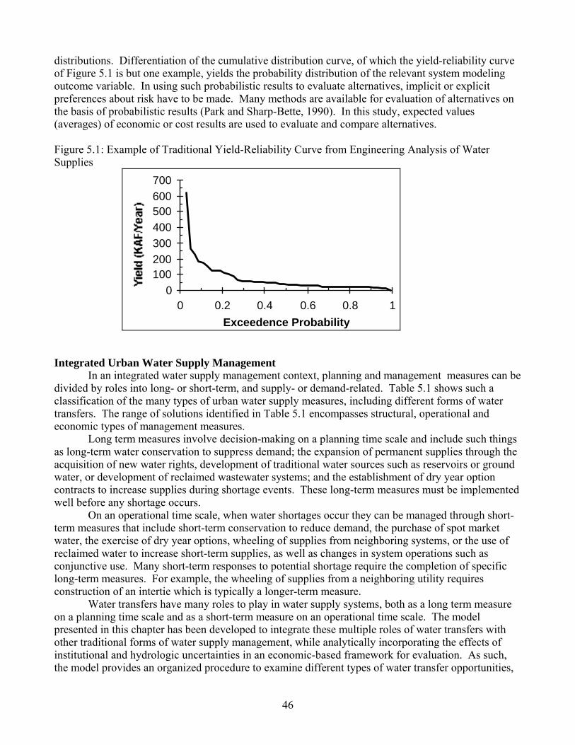
distributions. Differentiation of the cumulative distribution curve, of which the yield-reliability curve of Figure 5.1 is but one example, yields the probability distribution of the relevant system modeling outcome variable. In using such probabilistic results to evaluate alternatives, implicit or explicit preferences about risk have to be made. Many methods are available for evaluation of alternatives on the basis of probabilistic results (Park and Sharp-Bette, 1990). In this study, expected values (averages) of economic or cost results are used to evaluate and compare alternatives. Figure 5.1: Example of Traditional Yield-Reliability Curve from Engineering Analysis of Water Supplies

0100200300400500600700

0 0.2 0.4 0.6 0.8 1Exceedence Probability

Integrated Urban Water Supply Management In an integrated water supply management context, planning and management measures can be divided by roles into long- or short-term, and supply- or demand-related. Table 5.1 shows such a classification of the many types of urban water supply measures, including different forms of water transfers. The range of solutions identified in Table 5.1 encompasses structural, operational and economic types of management measures. Long term measures involve decision-making on a planning time scale and include such things as long-term water conservation to suppress demand; the expansion of permanent supplies through the acquisition of new water rights, development of traditional water sources such as reservoirs or ground water, or development of reclaimed wastewater systems; and the establishment of dry year option contracts to increase supplies during shortage events. These long-term measures must be implemented well before any shortage occurs. On an operational time scale, when water shortages occur they can be managed through short-term measures that include short-term conservation to reduce demand, the purchase of spot market water, the exercise of dry year options, wheeling of supplies from neighboring systems, or the use of reclaimed water to increase short-term supplies, as well as changes in system operations such as conjunctive use. Many short-term responses to potential shortage require the completion of specific long-term measures. For example, the wheeling of supplies from a neighboring utility requires construction of an intertie which is typically a longer-term measure. Water transfers have many roles to play in water supply systems, both as a long term measure on a planning time scale and as a short-term measure on an operational time scale. The model presented in this chapter has been developed to integrate these multiple roles of water transfers with other traditional forms of water supply management, while analytically incorporating the effects of institutional and hydrologic uncertainties in an economic-based framework for evaluation. As such, the model provides an organized procedure to examine different types of water transfer opportunities,

46

in the context of the associated uncertainties, for the integrated management of urban water supply system reliability. Chapter Overview This chapter is organized as follows. Section 2 presents an overview and diagram of the water supply reliability model structure. Sections 3 and 4 explain the details and workings of the two principal sub-models, dealing with supply system yield and shortage management, respectively. Section 5 explains how the sub-models are integrated with each other into a single model and describes the results produced from a single run. Section 6 explains the modeling process of using the integrated model in a routine to evaluate alternatives and the effects of institutional uncertainties. Section 7 concludes the presentation of the general modeling approach. 2. Overview of Integrated Water Supply Reliability Modeling For analysis and comprehension, the water supply reliability model is organized into two major components or sub-models, representing a separation between the management of physical water sources, i.e. permanent supplies and their operation to meet fixed demand in a predominantly planning context, versus the management of demand and short-term supplies under uncertain shortage in a predominantly operational context. Figure 5.2 shows the overall structure of the model. Part of the rationale for separating an urban water supply system this way is theoretical, based on whether the activity or decision affects the level of supply or of demand. The other part is convenience and adaptation to current practice in water supply modeling. The Water Supply Yield Sub-Model is based on conventional reliability modeling using simulation techniques whereas those activities in the Shortage Management Sub-Model are all amenable to linear optimization. The sub-model dealing with the operation of the permanent water sources is a simulation model of the physical supply system. Run on a planning time scale, the Water Supply Yield Sub-Model ('Yield sub-model') simulates the effects of long-term water supply augmentation decisions, including the integration of various forms of permanent transfers, on supply system reliability, given a set of system operating policies. The shortage event outcomes of the Yield sub-model, after transformation using the plotting position rule developed in Chapter 3, are passed to the Shortage Management Sub-Model ('Shortage sub-model'). This second sub-model is an optimization procedure that identifies the least cost mix of shortage and demand management decisions that accommodate the probability distribution of shortage from the Yield sub-model. The Shortage sub-model solves this problem using the two-stage linear programming approach presented in Chapter 4. Permanent types of water transfers, having a long term effect on the overall levels of water supply, are handled in the Yield sub-model, while contingent and temporary types of water transfers, conditioned on the possibility of shortages occurring, are handled in the Shortage Management sub-model. The two part integrated model is placed within a loop sequence to analytically integrate the effects of any probabilistic model parameters (of the supply system design and of the shortage management options) arising from important institutional uncertainties. The looped model routine is run to evaluate each set of planning alternatives and/or operating policies for the water supply system under study. Probabilistic performance results from the model, including the economic cost of meeting urban water supply system demand for each supply system alternative, can then be compared to identify preferred alternatives.

47

Table 5.1: Classification of Urban Integrated Water Supply System Management Measures and their Incorporation into Reliability Model Structure

LONG TERM MEASURES

SHORT TERM MEASURES

Supply

Supply

• Acquire permanent new water rights (S) • Develop ground water wells (S/O) • Construct surface water reservoirs (S) • Develop wastewater reclamation capacity (O) • Establish dry year option contracts for contingent water transfers (O) • Institute conjunctive operation of surface and ground water supplies (S)

• Apply hedging to reservoir operations (S)• Purchase water on the spot market (O) • Exercise dry year option contract (O) • Expand utilization of reclaimed water (O) • Purchase water from a water bank (O)

Demand

Demand

• Adopt long-term conservation, i.e. plumbing devices, xeriscaping, more water-efficient equipment (O) • Adjust water pricing rate structures (?) • Establish interruptable supply contracts for non-residential users (O)

• Adopt short-term conservation, i.e. reduce water-using activities, install temporary water-saving devices (O) • Reduce distribution pressure (?) • Interrupt demand to non-residential users (O) • Other measures for non-residential demand (?)

(S) : incorporated into the Supply Yield simulation sub-model; (O) : incorporated into the Shortage Management optimization sub-model; (?) : determined outside of the water supply reliability model or in an add-on or external sub-model.

48

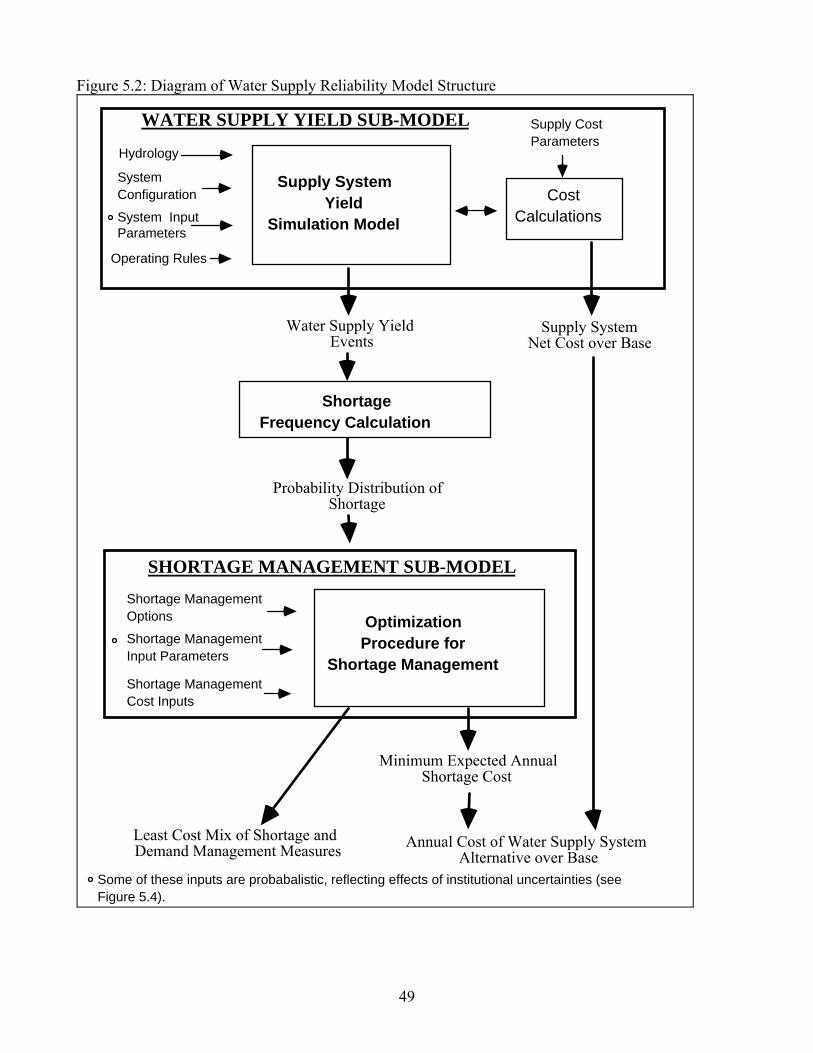
Figure 5.2: Diagram of Water Supply Reliability Model Structure

WATER SUPPLY YIELD SUB-MODEL

Water Supply Yield Events

Probability Distribution of Shortage

Supply System Net Cost over Base

Operating Rules

System Input Parameters

System Configuration

Hydrology

Supply System Yield

Simulation Model

Cost Calculations

Supply Cost Parameters

Minimum Expected Annual Shortage Cost

Annual Cost of Water Supply System Alternative over Base

Least Cost Mix of Shortage and Demand Management Measures

Shortage Frequency Calculation

SHORTAGE MANAGEMENT SUB-MODEL

Shortage Management Options

Shortage Management Input Parameters

Shortage Management Cost Inputs

Optimization Procedure for

Shortage Management

Some of these inputs are probabalistic, reflecting effects of institutional uncertainties (see Figure 5.4).

49

3. Water Supply Yield Sub-model Yield Modeling In the Water Supply Yield sub-model, permanent water transfers, involving the acquisition of permanent water rights or the long-term transfer of water, are integrated with the operation of traditional or existing sources of water to expand or manage supplies to meet some specified design demand. Typical water sources and management options included in this sub-model are those categorized as long-term and supply-related and for which integration into a systems analysis is best handled with simulation ('(S)' in Table 5.1). In this first part of the integrated model shown in Figure 5.2, the un-adjusted 'full' level of demand is used, reflecting the un-adjusted long-term planning expectation. The need for adjustments to demand, whether long or short-term, is handled separately in the subsequent Shortage Management sub-model. The core of the Yield sub-model is a simulation modeling procedure that computes a time-series of water shortage events relative to the target water demand, over the simulation period. The physical configuration of the supply system and its operating rules are mathematically represented in the model, which is run as a continuous simulation over the period of the stream flow record, using stream flow data and other input design parameters, some of which may be uncertain. The integration of permanent water transfers into an existing supply system will depend on the unique configuration of the physical system, on any feasible alternatives for construction of new infrastructure, on the choice of system operating procedures, on the type of water transfer arrangement, and on the physical and hydrologic characteristics of the source of the transferred water. Evaluating, under both hydrologic and institutional uncertainty, the many ways that permanent water transfers can be integrated into existing supply systems is usually too complex for direct optimization. Simulation provides a very straightforward, simple and highly flexible approach to explore and compare alternative supply strategies made up of combinations of long-term capital investment decisions and different operating rules. Most moderate to large urban water supply agencies already have such system yield simulation computer models, which can be built relatively easily in spreadsheet programs. Uncertain Yield Model Inputs Inputs for the Yield sub-model are the supply system physical configuration, including representation of infrastructure, facilities and natural water sources; the operating rules for this system; and the hydrologic and other system input parameters needed to run the simulation (see Table 5.2). Among these other system input parameters are some whose levels are highly uncertain as a consequence of institutional factors. In an extension to typical yield simulation models, marginal or net operating costs for the supply system (pumping, hydropower, treatment, etc.) also are included. The uncertain hydrology is represented by time series of stream flows that provide the sequence of uncertain inflow events to drive the simulation model. In the case of multiple inflows to the supply system, including flows associated with a permanent water transfer source, each inflow must be represented by a time-series over the same period. If long enough historical flow records exist for each inflow or most of them, it is preferable to use them directly in the simulation. The possibility of unrepresented extreme events (more severe droughts than recorded in the historical record) can be accounted for in the probability distribution of the resulting shortage events through the choice of a plotting position equation (Chapter 3). Institutional uncertainties arise from uncertainties in regulatory impacts, the evolution of environmental conflicts, legal outcomes, third party impacts, future economic growth, changes in technology, etc. (Chapter 2). These types of uncertainties can be translated into their probabilistic effects on the levels of various design parameters and/or the likely success/failure of infrastructure construction projects. For example, in a river reservoir operation, instream fish flow requirements may

50

be highly uncertain and dependent on long-term resolution of regional or local environmental issues (as in the Bay-Delta situation), or on future changes in regulatory policy and its implementation, on legal decisions related to water rights, etc. Rates of economic growth affect water use in a shared water resource system, such that in a planning context, the future level of availability of a surface water right entitlement, or of the production level from a well field may be uncertain. While the effects of hydrologic uncertainties are captured with a single simulation run of the Yield sub-model (in the distribution of shortage events), the effects of institutional factors on the integrated performance of the water supply system are evaluated in an analysis framework using the full integrated water supply model. The procedure is described later in Section 6. Operating Rules and Operation Costs Changes in operating rules associated with the water sources in the supply system can be investigated separately or jointly with other supply strategies by making appropriate changes to the simulation procedure inputs. For example, the use of hedging in reservoir operations, changes in ground water pumping schedules, or changes in the operation of conveyance structures are operating strategies that may improve supply system reliability in meeting demand. For a given physical supply system configuration, different operating strategies can be simulated on a planning time-scale in the Yield sub-model and their effects captured in changes to the shortage outcome events and to the operating costs of that system. Each given supply system design alternative has an associated marginal or net cost made up of new capital investments and changes in operations and maintenance which are calculated in the Yield sub-model for each simulation run. This calculation is carried out after first establishing a base case run of the Yield sub-model for the 'un-modified' supply system design configuration and its existing operating rules. Next, modifications to the base case Yield sub-model inputs are made for the given alternative design and the sub-model is run. These modifications might include one or more changes to the supply system design configuration, to supply system design parameters, or to operating rules (see Yield sub-model inputs in Figure 5.2 and Table 5.2). By comparing alternative and base case simulation results, net operations and maintenance costs (or savings) over base case operations can be identified and then converted to annualized operating and maintenance costs (savings) for the given alternative. The annualized capital investment costs for the alternative system design are determined independently of the simulation procedure, and based on estimated capital costs of any added infrastructure over base case.

51

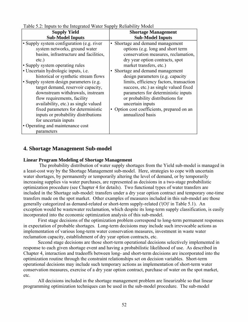
Table 5.2: Inputs to the Integrated Water Supply Reliability Model Supply Yield

Sub-Model Inputs Shortage Management

Sub-Model Inputs • Supply system configuration (e.g. river

system networks, ground water basins, infrastructure and facilities, etc.)

• Supply system operating rules • Uncertain hydrologic inputs, i.e.

historical or synthetic stream flows • Supply system design parameters (e.g.

target demand, reservoir capacity, downstream withdrawals, instream flow requirements, facility availability, etc.) as single valued fixed parameters for deterministic inputs or probability distributions for uncertain inputs

• Operating and maintenance cost parameters

• Shortage and demand management options (e.g. long and short term conservation measures, reclamation, dry year option contracts, spot market transfers, etc.)

• Shortage and demand management design parameters (e.g. capacity limits, efficiency factors, transaction success, etc.) as single valued fixed parameters for deterministic inputs or probability distributions for uncertain inputs

• Option cost coefficients, prepared on an annualized basis

4. Shortage Management Sub-model Linear Program Modeling of Shortage Management The probability distribution of water supply shortages from the Yield sub-model is managed in a least-cost way by the Shortage Management sub-model. Here, strategies to cope with uncertain water shortages, by permanently or temporarily altering the level of demand, or by temporarily increasing supplies via water purchases, are represented as decisions in a two-stage probabilistic optimization procedure (see Chapter 4 for details). Two functional types of water transfers are included in the Shortage sub-model: transfers under a dry year option contract and temporary one-time transfers made on the spot market. Other examples of measures included in this sub-model are those generally categorized as demand-related or short-term supply-related ('(O)' in Table 5.1). An exception would be wastewater reclamation, which despite its long-term supply classification, is easily incorporated into the economic optimization analysis of this sub-model. First stage decisions of the optimization problem correspond to long-term permanent responses in expectation of probable shortages. Long-term decisions may include such irrevocable actions as implementation of various long-term water conservation measures, investment in waste water reclamation capacity, establishment of dry year option contracts, etc. Second stage decisions are those short-term operational decisions selectively implemented in response to each given shortage event and having a probabilistic likelihood of use. As described in Chapter 4, interaction and tradeoffs between long- and short-term decisions are incorporated into the optimization routine through the constraint relationships set on decision variables. Short-term operational decisions may include such temporary actions as implementation of short-term water conservation measures, exercise of a dry year option contract, purchase of water on the spot market, etc. All decisions included in the shortage management problem are linearizable so that linear programming optimization techniques can be used in the sub-model procedure. The sub-model

52

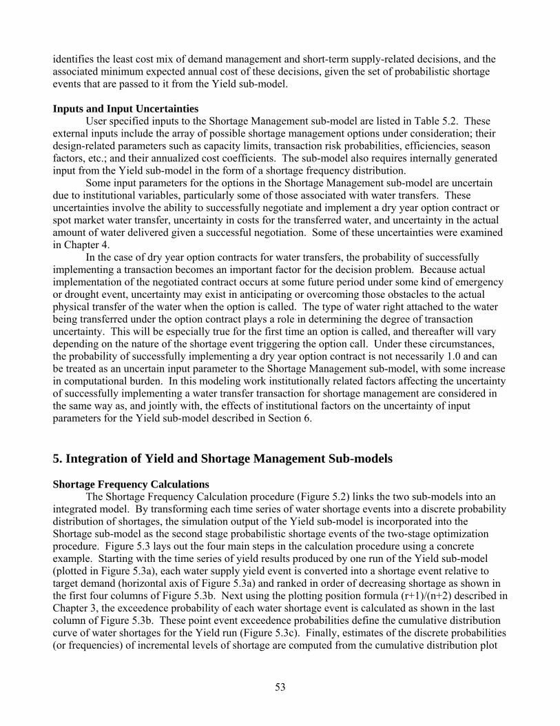
identifies the least cost mix of demand management and short-term supply-related decisions, and the associated minimum expected annual cost of these decisions, given the set of probabilistic shortage events that are passed to it from the Yield sub-model. Inputs and Input Uncertainties User specified inputs to the Shortage Management sub-model are listed in Table 5.2. These external inputs include the array of possible shortage management options under consideration; their design-related parameters such as capacity limits, transaction risk probabilities, efficiencies, season factors, etc.; and their annualized cost coefficients. The sub-model also requires internally generated input from the Yield sub-model in the form of a shortage frequency distribution. Some input parameters for the options in the Shortage Management sub-model are uncertain due to institutional variables, particularly some of those associated with water transfers. These uncertainties involve the ability to successfully negotiate and implement a dry year option contract or spot market water transfer, uncertainty in costs for the transferred water, and uncertainty in the actual amount of water delivered given a successful negotiation. Some of these uncertainties were examined in Chapter 4. In the case of dry year option contracts for water transfers, the probability of successfully implementing a transaction becomes an important factor for the decision problem. Because actual implementation of the negotiated contract occurs at some future period under some kind of emergency or drought event, uncertainty may exist in anticipating or overcoming those obstacles to the actual physical transfer of the water when the option is called. The type of water right attached to the water being transferred under the option contract plays a role in determining the degree of transaction uncertainty. This will be especially true for the first time an option is called, and thereafter will vary depending on the nature of the shortage event triggering the option call. Under these circumstances, the probability of successfully implementing a dry year option contract is not necessarily 1.0 and can be treated as an uncertain input parameter to the Shortage Management sub-model, with some increase in computational burden. In this modeling work institutionally related factors affecting the uncertainty of successfully implementing a water transfer transaction for shortage management are considered in the same way as, and jointly with, the effects of institutional factors on the uncertainty of input parameters for the Yield sub-model described in Section 6. 5. Integration of Yield and Shortage Management Sub-models Shortage Frequency Calculations The Shortage Frequency Calculation procedure (Figure 5.2) links the two sub-models into an integrated model. By transforming each time series of water shortage events into a discrete probability distribution of shortages, the simulation output of the Yield sub-model is incorporated into the Shortage sub-model as the second stage probabilistic shortage events of the two-stage optimization procedure. Figure 5.3 lays out the four main steps in the calculation procedure using a concrete example. Starting with the time series of yield results produced by one run of the Yield sub-model (plotted in Figure 5.3a), each water supply yield event is converted into a shortage event relative to target demand (horizontal axis of Figure 5.3a) and ranked in order of decreasing shortage as shown in the first four columns of Figure 5.3b. Next using the plotting position formula (r+1)/(n+2) described in Chapter 3, the exceedence probability of each water shortage event is calculated as shown in the last column of Figure 5.3b. These point event exceedence probabilities define the cumulative distribution curve of water shortages for the Yield run (Figure 5.3c). Finally, estimates of the discrete probabilities (or frequencies) of incremental levels of shortage are computed from the cumulative distribution plot

53

by linear interpolation and then simple differentiation (Figure 5.3d). The mid-point of the shortage interval is taken as the average magnitude for that shortage event. Discretization of the shortage events is a matter of choice, depending on technical limits of computing capacity, and consideration of water supply and shortage management operational characteristics. Integrated Model Results Model results produced by each integrated run are listed in Table 5.3 and described in the following paragraphs. Two types of results are produced by each Yield sub-model run, after transformation in the Shortage Frequency Calculation procedure. These are the probability distribution of annual (or other time increment selected as the basis of the supply simulation procedure) yield and the probability distribution of annual net operating costs over base case. From the yield reliability and operating cost data, other performance information can be computed. These include the average magnitude of shortage, or system deficit, per year; the likelihood (or marginal probability) of experiencing a shortage in any given year; and the average annual net operating cost. Results from the Shortage sub-model for each run are the least-cost mix of shortage management options, along with their optimal levels and expected annual cost of implementation. This cost can be understood as the minimum expected annual cost of supply yield failure (i.e. shortage) associated with the particular yield reliability realization for one given Supply Yield sub-model run. In fact, the yield reliability curve or its associated shortage frequency distribution is itself a stochastic distribution contingent on the joint effects of hydrologic and institutional uncertainty for one alternative combination of supply system configuration and operation. Each model run produces one empirical realization of this random shortage frequency distribution. Economic integration of the two sub-models is done by adding each of their separate cost components into a single annualized total cost. For a particular supply system alternative, each integrated model run produces a final system cost result (see Figure 5.2) composed of (a) fixed new capital investment costs of yield for the supply alternative, (b) expected net operations/maintenance costs (over base case) of yield for the supply alternative, and (c) the minimum expected annual cost of managing probabilistic shortages of yield using the optimally selected set of shortage management options and quantities. Overall, the final cost result can be thought of as a measure of the overall water supply cost for a given supply system alternative. Figure 5.3: Steps Used in Shortage Frequency Calculation Procedure Fig. 5.3 (a) Supply Yield Sub-Model Time Series Results

0

100,000

200,000

300,000

400,000

500,000600,000

700,000

800,000

900,000

1,000,000

Time Step (years)

54

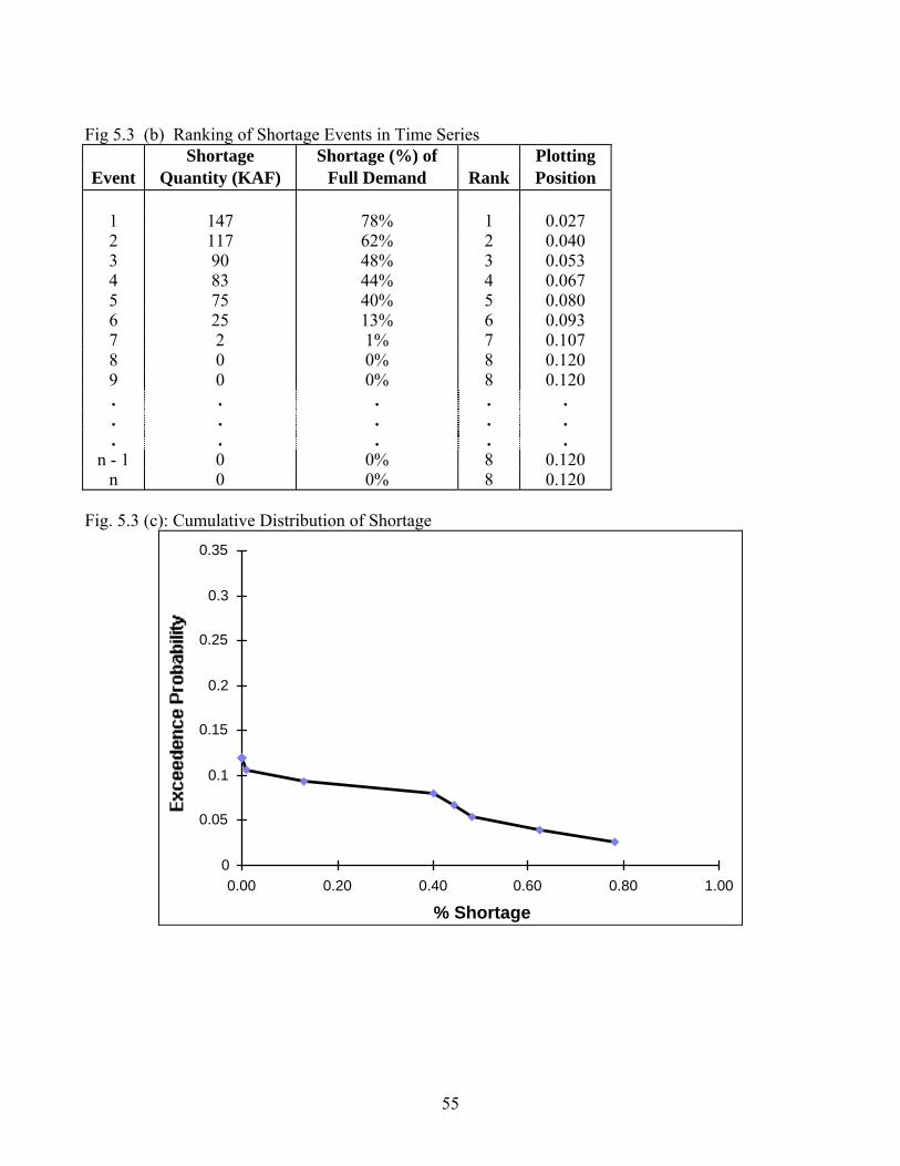
Fig 5.3 (b) Ranking of Shortage Events in Time Series

Shortage Shortage (%) of Plotting Event Quantity (KAF) Full Demand Rank Position

1 147 78% 1 0.027 2 117 62% 2 0.040 3 90 48% 3 0.053 4 83 44% 4 0.067 5 75 40% 5 0.080 6 25 13% 6 0.093 7 2 1% 7 0.107 8 0 0% 8 0.120 9 0 0% 8 0.120 . . . . . . . . . . . . . . .

n - 1 0 0% 8 0.120 n 0 0% 8 0.120

Fig. 5.3 (c): Cumulative Distribution of Shortage

0

0.05

0.1

0.15

0.2

0.25

0.3

0.35

0.00 0.20 0.40 0.60 0.80 1.00

% Shortage

55

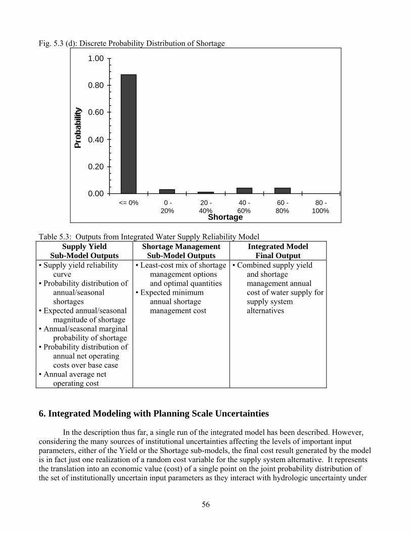
Fig. 5.3 (d): Discrete Probability Distribution of Shortage

0.00

0.20

0.40

0.60

0.80

1.00

<= 0% 0 -20%

20 -40%

40 -60%

60 -80%

80 -100%

Shortage Table 5.3: Outputs from Integrated Water Supply Reliability Model

Supply Yield Sub-Model Outputs

Shortage Management Sub-Model Outputs

Integrated Model Final Output

• Supply yield reliability curve

• Probability distribution of annual/seasonal shortages

• Expected annual/seasonal magnitude of shortage

• Annual/seasonal marginal probability of shortage

• Probability distribution of annual net operating costs over base case

• Annual average net operating cost

• Least-cost mix of shortage management options and optimal quantities

• Expected minimum annual shortage management cost

• Combined supply yield and shortage management annual cost of water supply for supply system alternatives

6. Integrated Modeling with Planning Scale Uncertainties In the description thus far, a single run of the integrated model has been described. However, considering the many sources of institutional uncertainties affecting the levels of important input parameters, either of the Yield or the Shortage sub-models, the final cost result generated by the model is in fact just one realization of a random cost variable for the supply system alternative. It represents the translation into an economic value (cost) of a single point on the joint probability distribution of the set of institutionally uncertain input parameters as they interact with hydrologic uncertainty under

56

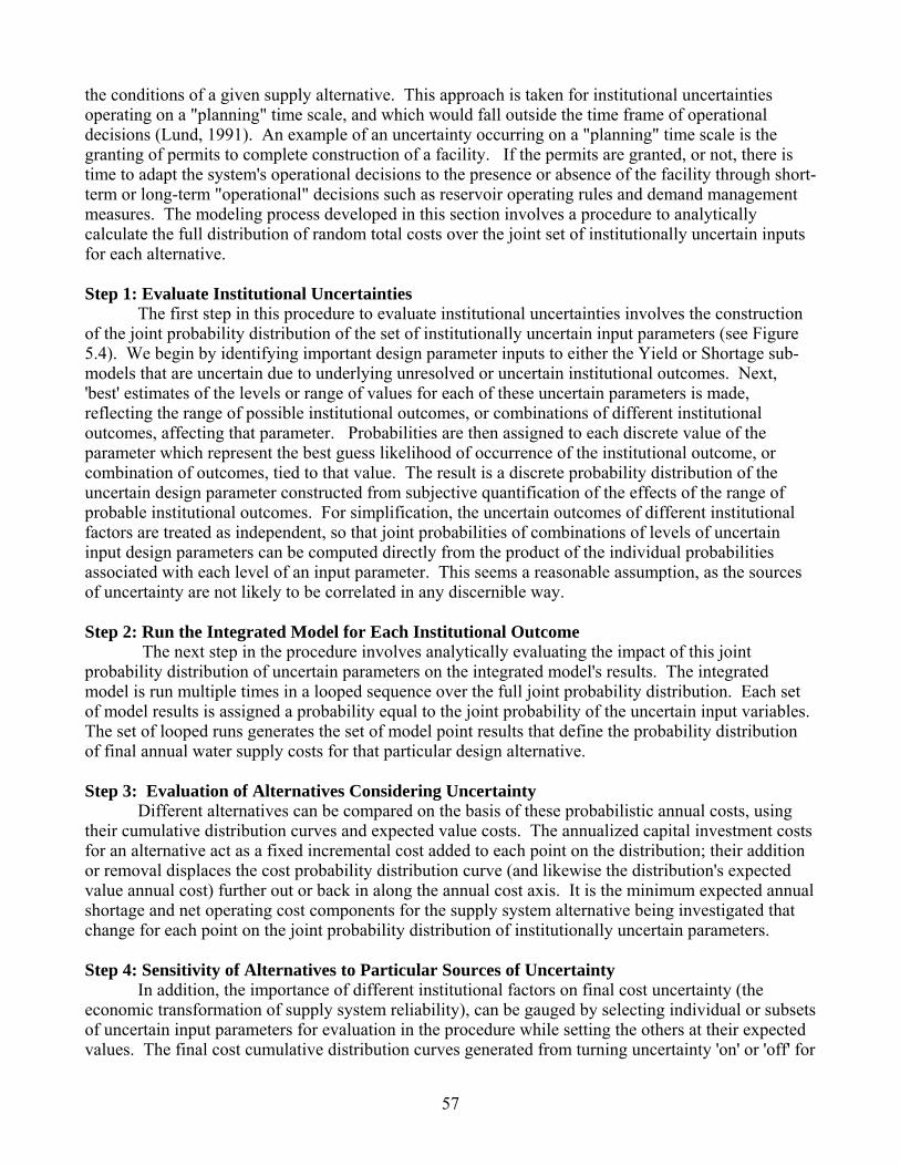
the conditions of a given supply alternative. This approach is taken for institutional uncertainties operating on a "planning" time scale, and which would fall outside the time frame of operational decisions (Lund, 1991). An example of an uncertainty occurring on a "planning" time scale is the granting of permits to complete construction of a facility. If the permits are granted, or not, there is time to adapt the system's operational decisions to the presence or absence of the facility through short-term or long-term "operational" decisions such as reservoir operating rules and demand management measures. The modeling process developed in this section involves a procedure to analytically calculate the full distribution of random total costs over the joint set of institutionally uncertain inputs for each alternative. Step 1: Evaluate Institutional Uncertainties The first step in this procedure to evaluate institutional uncertainties involves the construction of the joint probability distribution of the set of institutionally uncertain input parameters (see Figure 5.4). We begin by identifying important design parameter inputs to either the Yield or Shortage sub-models that are uncertain due to underlying unresolved or uncertain institutional outcomes. Next, 'best' estimates of the levels or range of values for each of these uncertain parameters is made, reflecting the range of possible institutional outcomes, or combinations of different institutional outcomes, affecting that parameter. Probabilities are then assigned to each discrete value of the parameter which represent the best guess likelihood of occurrence of the institutional outcome, or combination of outcomes, tied to that value. The result is a discrete probability distribution of the uncertain design parameter constructed from subjective quantification of the effects of the range of probable institutional outcomes. For simplification, the uncertain outcomes of different institutional factors are treated as independent, so that joint probabilities of combinations of levels of uncertain input design parameters can be computed directly from the product of the individual probabilities associated with each level of an input parameter. This seems a reasonable assumption, as the sources of uncertainty are not likely to be correlated in any discernible way. Step 2: Run the Integrated Model for Each Institutional Outcome The next step in the procedure involves analytically evaluating the impact of this joint probability distribution of uncertain parameters on the integrated model's results. The integrated model is run multiple times in a looped sequence over the full joint probability distribution. Each set of model results is assigned a probability equal to the joint probability of the uncertain input variables. The set of looped runs generates the set of model point results that define the probability distribution of final annual water supply costs for that particular design alternative. Step 3: Evaluation of Alternatives Considering Uncertainty Different alternatives can be compared on the basis of these probabilistic annual costs, using their cumulative distribution curves and expected value costs. The annualized capital investment costs for an alternative act as a fixed incremental cost added to each point on the distribution; their addition or removal displaces the cost probability distribution curve (and likewise the distribution's expected value annual cost) further out or back in along the annual cost axis. It is the minimum expected annual shortage and net operating cost components for the supply system alternative being investigated that change for each point on the joint probability distribution of institutionally uncertain parameters. Step 4: Sensitivity of Alternatives to Particular Sources of Uncertainty In addition, the importance of different institutional factors on final cost uncertainty (the economic transformation of supply system reliability), can be gauged by selecting individual or subsets of uncertain input parameters for evaluation in the procedure while setting the others at their expected values. The final cost cumulative distribution curves generated from turning uncertainty 'on' or 'off' for

57

selected subsets of institutionally driven input parameters can be compared, as well as each curve's expected value cost, to determine a relative measure of the economic cost of various sources of institutional uncertainty. Figure 5.4 shows a flow diagram of running the integrated model to evaluate the impacts of institutionally uncertain inputs to the Yield and Shortage sub-models for each design alternative. The diagram in Figure 5.4 shows how individual discrete probability distributions of uncertain input parameters are first combined into a joint probability distribution. This joint distribution is then evaluated in a sequence of looped model runs to generate a unique cumulative distribution function of annual costs for the alternative. The shape of the final cost probability distribution reflects the interaction of the effects of multiple sources of institutional uncertainty with hydrology on overall system cost for that alternative. The model process described here is not limited in the number of uncertain inputs, however, computational burden increases exponentially with the number of uncertain inputs that are jointly evaluated. For each alternative design, whether involving structural, operational or combinations of both types of features, the modeling process requires making iterations to the supply system design configuration and/or operating rules in the Supply Yield sub-model. The model is then run in the looped sequence, over the joint probability of uncertain inputs, to construct the unique cumulative distribution curve of annual costs for that alternative. Alternative strategies can be evaluated by comparing their cumulative distributions of annual costs using a variety of techniques from simple expected value, to stochastic dominance, mean-variance analysis (Park and Sharp-Bette, 1990) and others where risk preferences are included in the framework. By removing the capital cost component from the final integrated model cost result distributions, as suggested above, a maximum willingness to pay annually for capital improvements can be computed from the difference in the expected annual costs of alternatives with and without an infrastructure investment. For example, if construction of an aqueduct to convey new permanent water transfers is one alternative under investigation, the difference in the final annual cost cumulative distribution curves, based only on annual net operating and shortage management costs, (i.e. excluding the capital cost of construction), for the water supply system with and without the aqueduct can be computed to determine the maximum willingness to pay for this construction project.

58

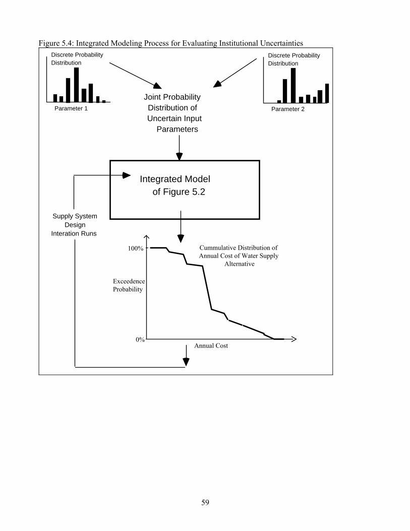
Figure 5.4: Integrated Modeling Process for Evaluating Institutional Uncertainties

Integrated Model of Figure 5.2

Discrete Probability Distribution

Parameter 1

Discrete Probability Distribution

Parameter 2

Joint Probability Distribution of Uncertain Input

Parameters

Supply System Design

Interation Runs

Cummulative Distribution of Annual Cost of Water Supply

Alternative

Annual Cost

Exceedence Probability

100%

0%

59

7. Conclusions Analytical consideration of the multiple uncertainties involved in water supply planning obviously is more complex than traditional consideration of hydrologic uncertainty. A rather complete and rigorous analytical procedure was presented in this chapter for evaluating the likely economic results of proposed water supply alternatives. This procedure includes a probabilistic economic optimization model for shortage management (the Shortage Management sub-model) and a simulation or optimization model of the water available for service area water demands (the Yield sub-model). These models are run jointly to allow joint examination of both hydrologic and multiple institutional uncertainties. In principle, this is an integrated water supply planning and management method which is both risk and economics based. The integrated approach presented is largely an extension of traditional yield modeling and water management studies and is based on information which is relatively common for most large urban water supply problems. The application of this approach is demonstrated in Chapter 6 for a simplified East Bay Municipal Utility District setting.

60

Chapter 6 Simplified Application

to the East Bay Municipal Utility District "The East Bay Municipal Utility District has a long record of investment choices which forego the lowest-cost source of design because of elements of uncertainty." Bain, et al. (1966, p. 369) 1. Introduction In this chapter, an application of the water supply reliability modeling framework (Chapter 5) to the East Bay Municipal Utility District (EBMUD) is presented. EBMUD is one of the larger, but less complex, urban water supply systems in California actively attempting to integrate various forms of water transfers, demand management, and yield enhancement into their system planning. EBMUD also faces multiple, complex, and interrelated institutional uncertainties critical in engineering its water supply system and water transfer activities that are typical of the present California water planning environment. As such, it provides an interesting and reasonably simple case study for 1) demonstrating and testing the modeling approach, 2) identifying data and input requirements, 3) interpreting various modeling results, and 4) developing a better understanding of the interactions of selected sources of institutional and hydrologic uncertainty and their impact on integrated urban water supply planning. East Bay Municipal Utility District Located on the east side of San Francisco Bay, EBMUD covers 310 square miles and serves roughly 1.1 million people in 20 incorporated cities and 15 unincorporated communities of Alameda and Contra Costa counties (EBMUD, 1995). Present normal-year demand is estimated at 215 million gallons per day (mgd) or 240,000 acre-feet per year (acft/yr). Forecasted demand for 2020 is 250 mgd or 280,000 acft/yr (EBMUD, 1991). The district receives almost all of its water from the Sierra Nevada Mountains' Mokelumne River Basin. The water supply system consists of a network of two large storage reservoirs on the Mokelumne River (Camanche and Pardee), three aqueducts conveying water from the Mokelumne reservoirs to its service area, five small terminal reservoirs within the service area, and six treatment plants (EBMUD, 1995). No ground water is presently used in the system. In addition to water rights and contracts for about 360,000 acft/yr (325 mgd) from the Mokelumne River, EBMUD has additional contract water rights with the U.S. Bureau of Reclamation's Central Valley Project for 150,000 acft/yr (134 mgd) from the American River. While EBMUD's expectation has been to divert this water through the Folsom South Canal via an extension south to its Mokelumne River aqueducts, current available access to American River water is via the Sacramento River and diversion at the Sacramento-San Joaquin Delta. Legal conflicts stemming from environmental concerns on the American River and in the Bay-Delta System continue to limit EBMUD's use of this water and prevent building the canal extension. An additional constraint to use through the Delta is the much lower quality of Delta water, compared to the extremely good quality of EBMUD's Mokelumne River source. Average annual runoff from the Mokelumne River is 720,000 acft. In 1976-77, the driest water year on record, annual runoff was 129,000 acft. For two consecutive years, runoff in 1987-88 was about 250,000 acft/yr and about 288,000 acft in 1991-92. System-wide cutbacks to all customers exceeded 35% (California Department of Water Resources, 1983) in 1977, and 15% in both 1987 and 1988 (California Department of Water Resources, 1993). Continued drought conditions resulted in

61

residential reductions of 20% in 1991-92 (CUWA, 1991; 1992). Storage in Camanche Reservoir reached its lowest level of 8,500 acft in 1988. To manage supply deficits, EBMUD has relied on conventional reservoir operations, water conservation programs and water rationing. At the same time, it has aggressively tried to implement several innovative forms of water transfers for shortage management, though with little success (Lund, et al., 1992). Conventional planning estimates of yield reliability, based on the present Mokelumne River supply system under a "most likely scenario" for 2020, indicate that EBMUD will face water supply shortages in 1 out of every 3 years on average (34% annual probability of shortage) and shortages equal to or exceeding 25% (70 TAF) in nearly 1 out of 10 years on average. They anticipate a "need-for-additional water" of 130 TAF/yr based on the worst expected supply shortfall (210 TAF in the worst year) during their most severe drought planning sequence (EDAW, Inc., 1992). However, there are many important non-hydrologic uncertainties in this scenario that affect yield reliability. A clear planning need exists to find strategies to reduce and manage anticipated and actual supply deficits for EBMUD. This chapter presents how the integrated reliability modeling and economic analysis framework developed for this research project can fulfill this planning need. Chapter Overview Section 2 describes potential roles for water transfers in the EBMUD system and identifies an initial subset selected to demonstrate the analytical approach for this application. Section 3 explains the setup and inputs for the EBMUD application, including a simplified representation of the physical configuration and operations of the EBMUD supply system, representation of the set of alternatives selected, and those shortage management options used in the modeling exercise. Because our purpose here is largely to demonstrate the modeling approach and potential policy implications, some simplifications were made to the actual EBMUD system. Important sources of institutional uncertainty in the context of EBMUD water transfer planning are discussed next in Section 4 along with their representation in various model input parameters as discrete probability distributions of those parameter values. Values used in the EBMUD modeling exercise for deterministic input parameters and cost coefficients are presented in Section 5. These values, while not unrealistic for urban water supplies in general, are not necessarily specific for the EBMUD. Model changes from the base case for each of the selected alternatives are also identified in this section. Section 6 presents and discusses the modeling results and their implications. The chapter concludes in Sections 7 and 8 with a summary of important methodological conclusions and lessons from the EBMUD model application. 2. Potential Roles for Water Transfers in EBMUD's System EBMUD's Water Transfer History During the 1976-77 drought, EBMUD gained its first experience transferring 25,000 acft of water from the American River via a diversion at the Delta (EBMUD, 1995). In the most recent California drought, EBMUD aggressively pursued three major efforts to transfer water, each of a different type (Lund et al., 1992). The first involved trading low quality Delta water for high quality Mokelumne River water in 1988 by pumping it upstream through one of EBMUD's aqueducts to its lower Mokelumne Reservoir (Camanche). The Delta water would replace Mokelumne River releases from the upper EBMUD Reservoir (Pardee) designated for downstream requirements, thus freeing an equivalent amount of water for EBMUD users. The transfer effort failed through lack of State approval due to the biological impacts and opposition by downstream users who had rights to the high quality Mokelumne water. The second effort, also in 1988, involved trying to set up dry year option contracts with downstream users on the Mokelumne River to purchase their higher priority water for EBMUD users. However, no transactions or transfers of water were completed. The last and final

62

attempt in early 1989 was similar to the 1976-77 water transfer; it succeeded. This transfer involved the purchase of 60,000 acft from the Yuba County Water Agency to be pumped directly from the Delta for treatment and use in EBMUD's service area. While the transaction succeeded, none of this water was actually used by EBMUD after unusually heavy March rains removed the immediate crisis. EBMUD resold the water to other buyers on the spot market. As evident from these attempts, water quality issues play an important part in EBMUD transfers. Motivation, due to customer preferences, treatment costs, and treatment capacities, is very strong to preserve the high quality of water entering the service area. EBMUD faces significant operational limitations on treating lower quality Delta water in its system. Existing treatment facilities would require major modifications to operations and possibly some infrastructure to accommodate frequent or substantial use of Delta water. EBMUD experienced limited success in negotiating water transfers during the last drought emergency. Nonetheless in the context of longer-term planning, the many types of water transfers offer significant opportunities for improving EBMUD's water supply system reliability. For this simplified application three forms of water transfers have been selected for evaluation. These are 1) integrating a permanent water transfer from the American River into the present supply system (based on EBMUD's Bureau of Reclamation contract); 2) establishing dry year option contracts with water sellers for water supplies during system deficits; and 3) purchasing spot market water during shortage events. Permanent Water Transfer A permanent or long-term transfer of contracted American River water could be integrated into EBMUD's present system in many ways, using a variety of different physical configurations and operational strategies. Diversion through the Delta would require no new conveyance infrastructure and was successfully used in the 1976-77 drought (Alternative "AR via DELTA"). However, impacts to water treatment operations would occur. In addition, use of water transfers via the Delta might be limited by the design of existing treatment facilities or might require additional treatment capacity designed for Delta quality water. However, extending the Folsom South Canal to convey higher quality American River water directly into EBMUD's aqueduct network would require capital investment but have minimal impact on treatment operations (Alternative "AR via CANAL"). High quality canal water could be operationally integrated into EBMUD's present system in three ways: (a) use the American River water as a direct back up or secondary supply source for EBMUD customers only; (b) use the water as the primary supply source, reserving more easily stored Mokelumne River water as a backup; and (c) build additional infrastructure to pump the American River water up to Camanche Reservoir (the lower one) to use for other releases, for storage and for EBMUD withdrawals. Other alternatives for using American River water in the EBMUD system could include ground water banking with conjunctive operation of surface and ground water supplies. In the present environment for water planning in California, any EBMUD alternative involving transferred American River water would involve significant institutional uncertainties, compounded by uncertainty about the future hydrologic relationship between the American and Mokelumne River flows. Identification of these uncertainties and their influences on levels of key system design parameters of the integrated model is presented in Chapter 5. Their impacts are treated in Section 4 of this chapter. Dry Year Options The second type of water transfer included in this application is dry year option contracts to provide access to additional water during shortage events. The EBMUD system has two distinct sources of water for contracting dry year options: senior water rights holders on the Mokelumne River and water sellers anywhere using Sacramento River or Delta water. The first source would provide

63

water of the same high quality as existing supplies through EBMUD's existing network of aqueducts. Water from this source would have a purchase cost, but few additional operating requirements over existing supplies. The second source of dry year option water transfers would entail low quality water withdrawals from the Delta if no additional conveyance facilities are constructed. Here additional treatment costs and treatment capacity would be involved. Spot Markets Spot market transfers or one-time purchases of water on the spot market are the last type of water transfer considered in this application. Sources of spot market water would be the same as those for dry year option contracts as well as some kind of drought emergency water bank. Treatment issues are the same as those for the dry year option sources. Many other possibilities for water transfers exist, some more obscure, less feasible or variations on those identified above. For example the exchange of low for high quality water that EBMUD attempted in 1988 is similar to the third way suggested above for operationally integrating a permanent transfer of American River water into EBMUD's supply system through the Folsom South Canal, pumping water into Camanche Reservoir. The water supply reliability modeling structure and framework of Chapter 5 is flexible, comprehensive and fully integrated to permit the evaluation of any of these water transfer possibilities. Modeled Water Transfer Alternatives For the application presented in this chapter, only a few representative alternatives for evaluating water transfers have been selected. Permanent transfer of American River water to the EBMUD system through either the Delta (Alternative AR via DELTA) or an extension of the Folsom South Canal (Alternative AR via CANAL) will be evaluated against base case operation (BASE). Both of these American River supply alternatives will be operated only as backup supply to the existing supplies in the Yield sub-model. In the context of shortage management, dry year option contracts and spot market purchases will be included as options, along with other non-transfer measures, in the optimization procedure of the Shortage Management sub-model. Consideration of two levels of water quality is made only in the specification of both dry year contract and spot market water transfers during shortage. The two levels are 'high' and 'low' and are distinguished by a need for additional treatment capacity beyond existing treatment operations (i.e., those designed for high quality Mokelumne River water). Modeling specifications for these water transfers in the EBMUD application are described in more detail later in this chapter. 3. Model of EBMUD's Supply System and Shortage Management This section describes the modeling of a simplified EBMUD system, including its supply system yield, shortage and demand management, and potential water transfers. A basic model (BASE) is first developed, and then modified to examine various planning alternatives and sources of institutional uncertainty. These alternatives are presented in later sections. Yield Sub-Model A simplified configuration of EBMUD's physical supply system appears in Figure 6.1. This configuration forms the basis of the Supply Yield sub-model for the BASE case and the two permanent water transfer alternatives. System components are identified on the map and listed by number in the first column of Table 6.1. Design parameters for the simulation procedure are grouped by component in the second column of Table 6.1. A brief description of each component appears in the last column.

64

The EBMUD integrated model developed for this application is a two season model, composed of a wet and a dry season each year. The period November to March and the period April to October constitute these two seasons, respectively. This choice of periods permits a more realistic simulation of river-reservoir operations with annual drawdown-refill cycle under the temporal pattern of California's hydrology, which is the case for EBMUD's Mokelumne water supply system. It also reflects a compromise to simplify model complexity, reduce data requirements and minimize computational burden in this initial application while still retaining important features of supply system behavior caused by extremes in monthly variability which would get averaged out in annual models. The following components comprise the physical parts of the EBMUD BASE case supply system. EBMUD's seven reservoirs have been combined into a single reservoir located on the Mokelumne River with 720,000 acft of active storage capacity (component 2). Inflow to the reservoir (component 1) is the historical monthly unimpaired flow record for the Mokelumne River (California Department of Water Resources, 1995) for 1921-1993. Instream flow requirements (component 4) consist of Mokelumne reservoir releases for fish (18,300 acft/yr average), channel losses (70,000 acft/yr estimated) and meeting Bay/Delta water quality standards (EBMUD, 1991). A single river withdrawal point (component 5) labeled "Downstream Withdrawals" is used to represent all Mokelumne River withdrawals and users, both up and downstream of EBMUD's reservoirs, having entitlements of higher priority than EMBUD's. This quantity includes entitlements for the Jackson Valley Irrigation District (3,850 acft/yr), the North San Joaquin Water Conservation District (20,000 acft/yr), the Woodbridge Irrigation District (60,000 acft/yr), and riparian and other senior appropriative water rights holders (21,000 acft/yr estimated) (EBMUD, 1991). EBMUD withdrawals (component 6) are based on meeting a target demand of 280,000 acft/yr for the 2020 planning scenario. Monthly requirements are based on the current average fraction of annual deliveries made in each month to EBMUD (California Department of Water Resources, 1994). Additional components of the BASE case are needed to model the integration of a permanent transfer of American River water under the two selected alternatives. These consist of runoff or flow for the American River (component 7) represented by the monthly historical unimpaired streamflow (California Department of Water Resources, 1995) for 1921-1993, a diversion point at the Folsom South Canal and its extension and tie-in to EBMUD's aqueducts (component 8) for Alternative AR via CANAL, a diversion point in the Delta at EBMUD's service area (component 10) for Alternative AR via DELTA, minimum instream flow requirements in the American River for fish flows, senior appropriators, channel losses and meeting Bay/Delta quality standards before EBMUD can make diversions at either point (component 9), and consideration of EBMUD water treatment facility constraints (component 11) on treating low quality water from the Delta for Alternative AR via DELTA. The BASE supply system and both permanent water transfer alternatives are operated using a linear hedging operation rule (component 3) for making releases from the Mokelumne River reservoir. The operating rule allows modification for two simple hedging features, one consisting of wet season carryover storage triggered by low forecasted inflow in the dry season, and the other consisting of a reduced dry season drawdown rate of storage triggered by low projected end-of-period storage. No consideration has been given to flood control, hydropower or terminal storage regulation of and inflows into the 5 terminal reservoirs in this simplified operating rule developed for our model application.

65

Figure 6.1: Map of EBMUD Simplified Water Supply System and American River Alternatives

66

American River

Sacramento River

South Folsom Canal

Mokelumne River

Camanche/Pardee Reservoirs (2,3)

EBMUD Aqueducts

DeltaInstream Flow Requirements

Instream Flow Requirements

Downstream Withdrawals

Delta Withdrawals to EBMUD

(1)

(5)(4)

(6)

(7)

(8)

(9)

(10)

(11)EBMUD Service Area

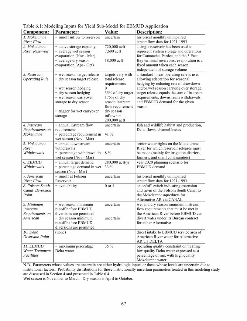
Table 6.1: Modeling Inputs for Yield Sub-Model for EBMUD Application Component: Parameter: Value: Description: 1. Mokelumne River Flow

• runoff inflow to reservoir uncertain historical monthly unimpaired streamflow data for 1921-1993

2. Mokelumne River Reservoir

• active storage capacity • average wet season evaporation (Nov - Mar) • average dry season evaporation (Apr - Oct)

720,000 acft 7,600 acft 18,000 acft

a single reservoir has been used to represent system storage and operations for Camanche, Pardee, and the 5 East Bay terminal reservoirs; evaporation is a fixed amount taken each season independent of storage volume

3. Reservoir Operating Rule

• wet season target release • dry season target release • wet season hedging • dry season hedging • wet season carryover storage to dry season • trigger for wet carryover storage

targets vary with total release requirements 0 35% of dry target175% of dry season instream flow requirement dry season inflow <= 200,000 acft

a standard linear operating rule is used allowing adaptation for seasonal hedging by reducing rate of drawdown and/or wet season carrying over storage; target release equals the sum of instream requirements, downstream withdrawals and EBMUD demand for the given season

4. Instream Requirements on Mokelumne

• annual instream flow requirements • percentage requirement in wet season (Nov - Mar)

uncertain 41 %

fish and wildlife habitat and production, Delta flows, channel losses

5. Mokelumne River Withdrawals

• annual downstream withdrawals • percentage withdrawal in wet season (Nov - Mar)

uncertain 8 %

senior water rights on the Mokelumne River for which reservoir releases must be made (mainly for irrigation districts, farmers, and small communities)

6. EBMUD Withdrawals

• annual target demand • percentage demand in wet season (Nov - Mar)

280,000 acft/yr 33 %

year 2020 planning scenario for EBMUD demand

7. American River Flow

• runoff at Folsom Reservoir

uncertain historical monthly unimpaired streamflow data for 1921-1993

8. Folsom South Canal Diversion Point

• availability 0 or 1 an on/off switch indicating extension and tie-in of the Folsom South Canal to the Mokelumne aqueducts for Alternative AR via CANAL

9. Minimum Instream Requirements on American

• wet season minimum runoff before EBMUD diversions are permitted • dry season minimum runoff before EBMUD diversions are permitted

uncertain uncertain

wet and dry season minimum instream flow requirements that must be met in the American River before EBMUD can divert water under its Bureau contract for either Alternative

10. Delta Diversion Point

(none) direct intake to EBMUD service area of American River water for Alternative AR via DELTA

11. EBMUD Water Treatment Facilities

• maximum percentage Delta water

35 % operating quality constraint on treating low quality Delta water expressed as a percentage of mix with high quality Mokelumne water

N.B. Parameters whose values are uncertain are either hydrologic inputs or those whose levels are uncertain due to institutional factors. Probability distributions for those institutionally uncertain parameters treated in this modeling study are discussed in Section 4 and presented in Table 6.4. Wet season is November to March. Dry season is April to October.

67

Shortage Management Sub-Model The Shortage Management sub-model is used to determine the least-expected value cost combination of long term and short term alternatives required to meet demand given a set of yield sub-model shortage frequency results. Long term and short term management options for the simplified EBMUD Shortage Management sub-model are listed in the first column of Table 6.2. Design parameters for setting up the optimization problem are given in the second column, followed by a brief description of the option/measure in the last column. A more comprehensive description of the alternatives and optimization equations appears in Chapter 4, under the base model. Long term measures considered are water treatment capacity expansion, dry year option contracts, long-term conservation, and water reuse. Long term conservation efforts include xeriscaping and plumbing retrofits. Water treatment capacity can be expanded as a long term measure to increase the quantity of transferred water under dry year option contracts or spot market purchases. Long term decisions are annual decisions (units of TAF/year) with the exception of dry year option contracts which can vary seasonally reflecting the seasonal timing of transfer activation (units of TAF/season). Short term measures include conservation, activating dry year options, and purchasing spot market water. Conservation measures include reducing lawn watering and reducing in-house water uses. Short term decisions are event- and season-specific decisions in response to shortage events and have units of TAF/event/season. The availability or effectiveness of the short term shortage management measures depends directly on the selection and levels of long term measures put in place. For instance, as more long term conservation is implemented, the effectiveness of short term conservation will decrease. This is sometimes referred to as "demand hardening". The available level of lawn watering reduction in response to a shortage is proportionally reduced with the level of long term xeriscaping attained. Lawn watering reduction is divided into two segments to reflect the severity of implementing high water reductions. Lawn watering reduction I is first implemented, followed by lawn water reduction II at a much higher cost. Ability to reduce in-house water uses to temporarily suppress demand is restricted by the level of reduction achieved from long term water fixture retrofitting. For each shortage level, the amount of dry year option activated is limited by the long term decision of the dry year option contract. The quantity of spot market water that can be purchased is dependent on the available water treatment capacity and amount already obtained through dry year options. The mathematical representation of these relationships between long term and short term alternatives is presented in Chapter 4.

68

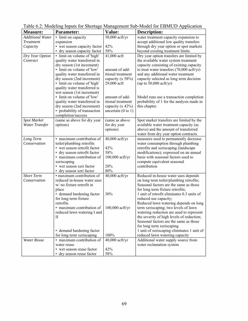
Table 6.2: Modeling Inputs for Shortage Management Sub-Model for EBMUD Application Measure: Parameter: Value: Description: Additional Water Treatment Capacity

• limit on capacity expansion • wet season capacity factor• dry season capacity factor

50,000 acft/yr 42% 58%

water treatment capacity expansion to accept additional low quality transfers through dry year option or spot markets beyond existing treatment limits

Dry Year Option Contract

• limit on volume of 'high' quality water transferred in dry season (1st increment) • limit on volume of 'low' quality water transferred in dry season (2nd increment) • limit on volume of 'high' quality water transferred is wet season (1st increment) • limit on volume of 'low' quality water transferred in dry season (2nd increment) • probability of transaction completion/success

41,000 acft amount of add-itional treatment capacity (x 58%) 29,000 acft amount of add-itional treatment capacity (x 42%) uncertain (0 to 1)

Dry year option transfers are limited by the available water system treatment capacity consisting of existing capacity to treat water transfers (70,000 acft/yr) and any additional water treatment capacity selected as long term decision (up to 50,000 acft/yr) Model runs use a transaction completion probability of 1 for the analysis made in this chapter.

Spot Market Water Transfer

(same as above for dry year options)

(same as above for dry year options)

Spot market transfers are limited by the available water treatment capacity (as above) and the amount of transferred water from dry year option contracts.

Long Term Conservation

• maximum contribution of toilet/plumbing retrofits • wet season retrofit factor • dry season retrofit factor • maximum contribution of xeriscaping • wet season xeri factor • dry season xeri factor

40,000 acft/yr 42% 58% 100,000 acft/yr 20% 80%

measures used to permanently decrease water consumption through plumbing retrofits and xeriscaping (landscape modifications); expressed on an annual basis with seasonal factors used to compute equivalent seasonal contribution

Short Term Conservation

• maximum contribution of reduced in-house water uses w/ no fixture retrofit in place • demand hardening factor for long term fixture retrofits • maximum contribution of reduced lawn watering I and II • demand hardening factor for long term xeriscaping

40,000 acft/yr 30% 100,000 acft/yr 100%

Reduced in-house water uses depends on long term toilet/plumbing retrofits; Seasonal factors are the same as those for long term fixture retrofits; 1 unit of retrofit eliminates 0.3 units of reduced use capacity; Reduced lawn watering depends on long term xeriscaping; two levels of lawn watering reduction are used to represent the severity of high levels of reduction; Seasonal factors are the same as those for long term xeriscaping 1 unit of xeriscaping eliminates 1 unit of reduced lawn watering capacity

Water Reuse • maximum contribution of water reuse • wet season reuse factor • dry season reuse factor

40,000 acft/yr 42% 58%

Additional water supply source from water reclamation system

69

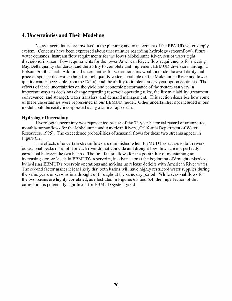
4. Uncertainties and Their Modeling Many uncertainties are involved in the planning and management of the EBMUD water supply system. Concerns have been expressed about uncertainties regarding hydrology (streamflow), future water demands, instream flow requirements for the lower Mokelumne River, senior water right diversions, instream flow requirements for the lower American River, flow requirements for meeting Bay/Delta quality standards, and the ability to complete and implement EBMUD diversions through a Folsom South Canal. Additional uncertainties for water transfers would include the availability and price of spot-market water (both for high quality waters available on the Mokelumne River and lower quality waters accessible from the Delta), and the ability to implement dry year option contracts. The effects of these uncertainties on the yield and economic performance of the system can vary in important ways as decisions change regarding reservoir operating rules, facility availability (treatment, conveyance, and storage), water transfers, and demand management. This section describes how some of these uncertainties were represented in our EBMUD model. Other uncertainties not included in our model could be easily incorporated using a similar approach. Hydrologic Uncertainty Hydrologic uncertainty was represented by use of the 73-year historical record of unimpaired monthly streamflows for the Mokelumne and American Rivers (California Department of Water Resources, 1995). The exceedence probabilities of seasonal flows for these two streams appear in Figure 6.2. The effects of uncertain streamflows are diminished when EBMUD has access to both rivers, as seasonal peaks in runoff for each river do not coincide and drought low flows are not perfectly correlated between the two basins. The first factor allows for the possibility of maintaining or increasing storage levels in EBMUD's reservoirs, in advance or at the beginning of drought episodes, by hedging EBMUD's reservoir operations and making up release deficits with American River water. The second factor makes it less likely that both basins will have highly restricted water supplies during the same years or seasons in a drought or throughout the same dry period. While seasonal flows for the two basins are highly correlated, as illustrated in Figures 6.3 and 6.4, the imperfection of this correlation is potentially significant for EBMUD system yield.

70

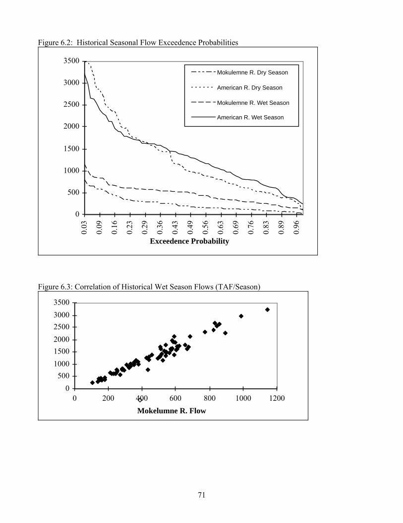
Figure 6.2: Historical Seasonal Flow Exceedence Probabilities

0

500

1000

1500

2000

2500

3000

3500

0.03

0.09

0.16

0.23

0.29

0.36

0.43

0.49

0.56

0.63

0.69

0.76

0.83

0.89

0.96

Exceedence Probability

Mokulemne R. Dry Season

American R. Dry Season

Mokulemne R. Wet Season

American R. Wet Season

Figure 6.3: Correlation of Historical Wet Season Flows (TAF/Season)

0500

100015002000250030003500

0 200 400 600 800 1000 1200Mokelumne R. Flow

A i Ri Fl

71

Figure 6.4: Correlation of Historical Dry Season Flows (TAF/season)

0500

100015002000250030003500

0 200 400 600 800Mokelumne R. Flow

Institutional Uncertainties in the Supply Yield Sub-model Three major effects of various institutional uncertainties are represented in the current EBMUD model for the supply system. These are annual instream flow requirements on the lower Mokelumne River (IFR), annual senior right withdrawals from the Mokelumne River (DSW), and dry season minimum instream flows required on the lower American River (IA2Min). These three parameters were initially identified as highly uncertain and thought to have the most significant effects on supply system yield under the BASE case and the two alternatives. In the assignment of values for each of these parameters, uncertainty about numerous unresolved institutional issues and evolving outcomes in the EBMUD context, including some important pending legal and regulatory proceedings, is considered in estimating the likely range and occurrence of those values. Thus, relevant institutional uncertainties are incorporated into the Supply Yield sub-model by varying parameters in the system's operating rules and weighting the yield results according to the joint probability of the parameter set (following the approach described in Chapter 5). The impacts of institutional uncertainties on the three Yield sub-model parameter values are represented as probability distributions over a range of values taken from the literature for the likely range of institutional outcomes. For computational simplicity, five levels were chosen for each parameter affected by uncertainty. The assignment of probability values for each level is necessarily subjective, but is based on scenarios examined in recent technical studies. These uncertainties are discussed below, with probability values listed in Table 6.3. IFR - Lower Mokelumne River Instream Flow Requirements Over a planning horizon relevant for facility planning and operations studies, instream flow requirements for the lower Mokelumne River are highly uncertain. These uncertainties are driven by environmental regulations and California Department of Fish and Game implementation of those regulations, by eventual implementation of Bay/Delta water quality standards, and by other developments on the Mokelumne River affecting inflow levels (EDAW, Inc., 1992). The range of potential values for this annual instream flow requirement is taken to be 32-131 TAF, based on numbers given in various EBMUD reports, and the most likely value is 105 TAF/yr. This requirement is disaggregated into seasonal values for modeling. The assignment of probabilities appearing in Table

72

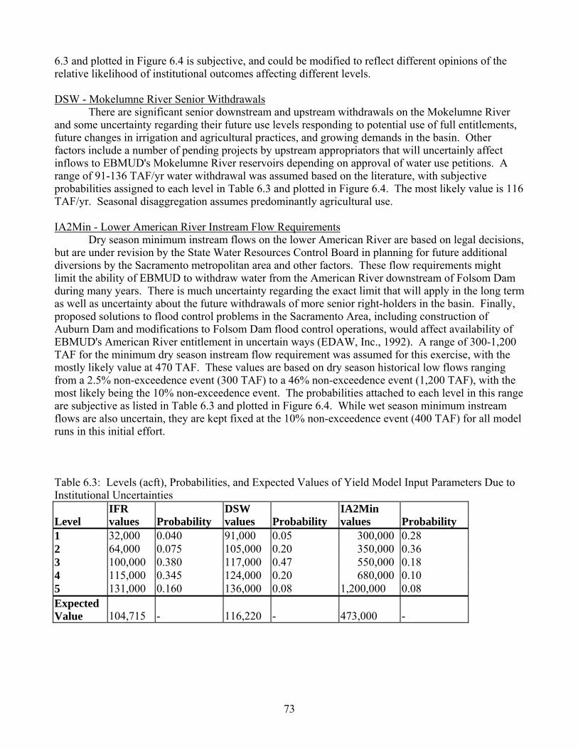
6.3 and plotted in Figure 6.4 is subjective, and could be modified to reflect different opinions of the relative likelihood of institutional outcomes affecting different levels. DSW - Mokelumne River Senior Withdrawals There are significant senior downstream and upstream withdrawals on the Mokelumne River and some uncertainty regarding their future use levels responding to potential use of full entitlements, future changes in irrigation and agricultural practices, and growing demands in the basin. Other factors include a number of pending projects by upstream appropriators that will uncertainly affect inflows to EBMUD's Mokelumne River reservoirs depending on approval of water use petitions. A range of 91-136 TAF/yr water withdrawal was assumed based on the literature, with subjective probabilities assigned to each level in Table 6.3 and plotted in Figure 6.4. The most likely value is 116 TAF/yr. Seasonal disaggregation assumes predominantly agricultural use. IA2Min - Lower American River Instream Flow Requirements Dry season minimum instream flows on the lower American River are based on legal decisions, but are under revision by the State Water Resources Control Board in planning for future additional diversions by the Sacramento metropolitan area and other factors. These flow requirements might limit the ability of EBMUD to withdraw water from the American River downstream of Folsom Dam during many years. There is much uncertainty regarding the exact limit that will apply in the long term as well as uncertainty about the future withdrawals of more senior right-holders in the basin. Finally, proposed solutions to flood control problems in the Sacramento Area, including construction of Auburn Dam and modifications to Folsom Dam flood control operations, would affect availability of EBMUD's American River entitlement in uncertain ways (EDAW, Inc., 1992). A range of 300-1,200 TAF for the minimum dry season instream flow requirement was assumed for this exercise, with the mostly likely value at 470 TAF. These values are based on dry season historical low flows ranging from a 2.5% non-exceedence event (300 TAF) to a 46% non-exceedence event (1,200 TAF), with the most likely being the 10% non-exceedence event. The probabilities attached to each level in this range are subjective as listed in Table 6.3 and plotted in Figure 6.4. While wet season minimum instream flows are also uncertain, they are kept fixed at the 10% non-exceedence event (400 TAF) for all model runs in this initial effort. Table 6.3: Levels (acft), Probabilities, and Expected Values of Yield Model Input Parameters Due to Institutional Uncertainties Level

IFR values

Probability

DSW values

Probability

IA2Min values

Probability

1 32,000 0.040 91,000 0.05 300,000 0.28 2 64,000 0.075 105,000 0.20 350,000 0.36 3 100,000 0.380 117,000 0.47 550,000 0.18 4 115,000 0.345 124,000 0.20 680,000 0.10 5 131,000 0.160 136,000 0.08 1,200,000 0.08 Expected Value

104,715

-

116,220

-

473,000

-

73

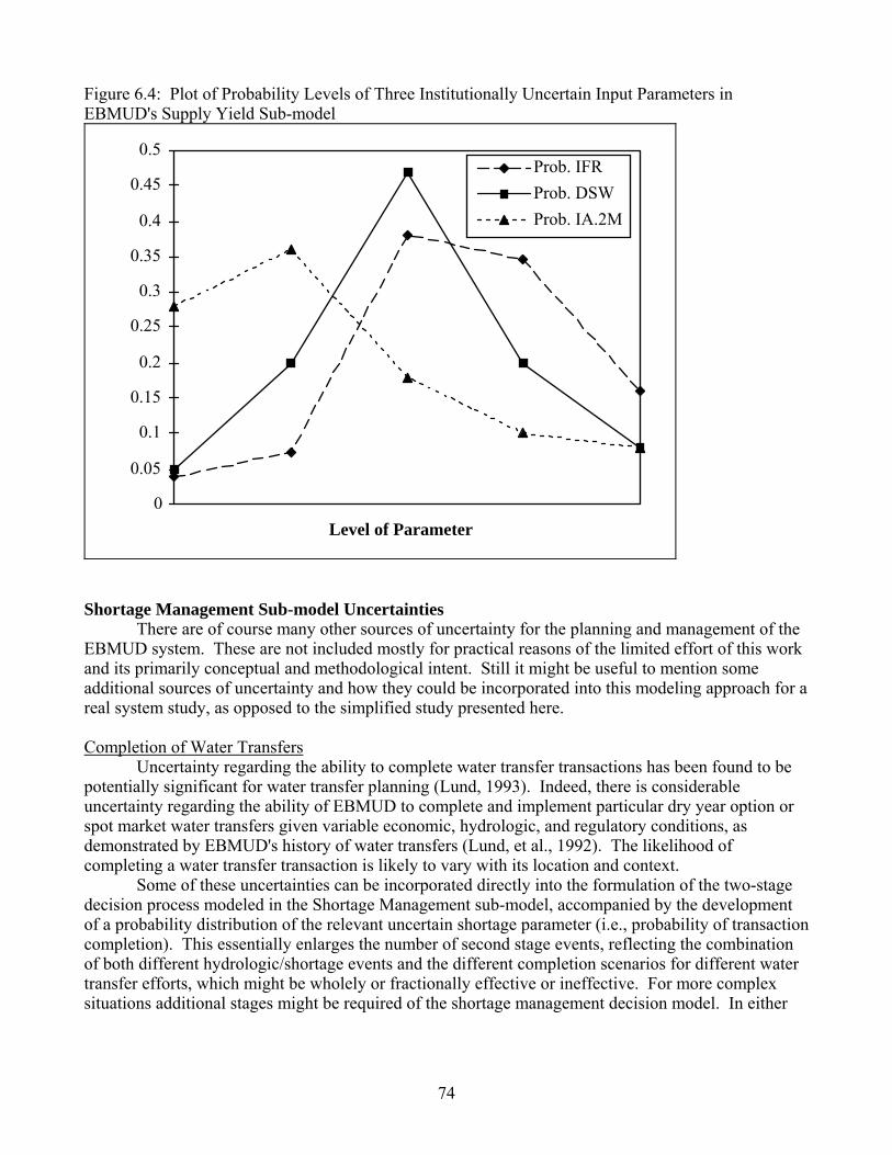
Figure 6.4: Plot of Probability Levels of Three Institutionally Uncertain Input Parameters in EBMUD's Supply Yield Sub-model

0

0.05

0.1

0.15

0.2

0.25

0.3

0.35

0.4

0.45

0.5

Level of Parameter

Prob. IFRProb. DSWProb. IA.2M

Shortage Management Sub-model Uncertainties There are of course many other sources of uncertainty for the planning and management of the EBMUD system. These are not included mostly for practical reasons of the limited effort of this work and its primarily conceptual and methodological intent. Still it might be useful to mention some additional sources of uncertainty and how they could be incorporated into this modeling approach for a real system study, as opposed to the simplified study presented here. Completion of Water Transfers Uncertainty regarding the ability to complete water transfer transactions has been found to be potentially significant for water transfer planning (Lund, 1993). Indeed, there is considerable uncertainty regarding the ability of EBMUD to complete and implement particular dry year option or spot market water transfers given variable economic, hydrologic, and regulatory conditions, as demonstrated by EBMUD's history of water transfers (Lund, et al., 1992). The likelihood of completing a water transfer transaction is likely to vary with its location and context. Some of these uncertainties can be incorporated directly into the formulation of the two-stage decision process modeled in the Shortage Management sub-model, accompanied by the development of a probability distribution of the relevant uncertain shortage parameter (i.e., probability of transaction completion). This essentially enlarges the number of second stage events, reflecting the combination of both different hydrologic/shortage events and the different completion scenarios for different water transfer efforts, which might be wholely or fractionally effective or ineffective. For more complex situations additional stages might be required of the shortage management decision model. In either

74

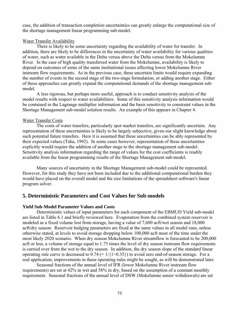
case, the addition of transaction completion uncertainties can greatly enlarge the computational size of the shortage management linear programming sub-model. Water Transfer Availability There is likely to be some uncertainty regarding the availability of water for transfer. In addition, there are likely to be differences in the uncertainty of water availability for various qualities of water, such as water available in the Delta versus above the Delta versus from the Mokelumne River. In the case of high quality transferred water from the Mokelumne, availability is likely to depend on outcomes of some of the same institutional issues affecting lower Mokelumne River instream flow requirements. As in the previous case, these uncertain limits would require expanding the number of events in the second stage of the two-stage formulation, or adding another stage. Either of these approaches can greatly expand the computational demands of the shortage management sub-model. A less rigorous, but perhaps more useful, approach is to conduct sensitivity analysis of the model results with respect to water availabilities. Some of this sensitivity analysis information would be contained in the Lagrange multiplier information and the basis sensitivity to constraint values in the Shortage Management sub-model solution results. An example of this appears in Chapter 4. Water Transfer Costs The costs of water transfers, particularly spot market transfers, are significantly uncertain. Any representation of these uncertainties is likely to be largely subjective, given our slight knowledge about such potential future transfers. Here it is assumed that these uncertainties can be ably represented by their expected values (Taha, 1992). In some cases however, representation of these uncertainties explicitly would require the addition of another stage to the shortage management sub-model. Sensitivity analysis information regarding the range of values for the cost coefficients is readily available from the linear programming results of the Shortage Management sub-model. Many sources of uncertainty in the Shortage Management sub-model could be represented. However, for this study they have not been included due to the additional computational burden they would have placed on the overall model and the size limitations of the spreadsheet software's linear program solver. 5. Deterministic Parameters and Cost Values for Sub-models Yield Sub-Model Parameter Values and Costs Deterministic values of input parameters for each component of the EBMUD Yield sub-model are listed in Table 6.1 and briefly reviewed here. Evaporation from the combined system reservoir is modeled as a fixed volume lost from storage, having a value of 7,600 acft/wet season and 18,000 acft/dry season. Reservoir hedging parameters are fixed at the same values in all model runs, unless otherwise stated, at levels to avoid storage dropping below 100,000 acft most of the time under the most likely 2020 scenario. When dry season Mokelumne River streamflow is forecasted to be 200,000 acft or less, a volume of storage equal to 1.75 times the level of dry season instream flow requirements is carried over from the wet to the dry season. In addition, the dry season slope of the standard linear operating rule curve is decreased to 0.74 (= 1/{1+0.35}) to avoid zero end-of-season storage. For a real application, improvements in these operating rules might be sought, as will be demonstrated later. Seasonal fractions of the annual level of IFR (lower Mokelumne River instream flow requirements) are set at 42% in wet and 58% in dry, based on the assumption of a constant monthly requirement. Seasonal fractions of the annual level of DSW (Mokelumne senior withdrawals) are set

75

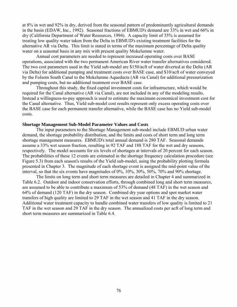
at 8% in wet and 92% in dry, derived from the seasonal pattern of predominantly agricultural demands in the basin (EDAW, Inc., 1992). Seasonal fractions of EBMUD's demand are 33% in wet and 66% in dry (California Department of Water Resources, 1994). A capacity limit of 35% is assumed for treating low quality water taken from the Delta in EBMUD's existing treatment facilities for the alternative AR via Delta. This limit is stated in terms of the maximum percentage of Delta quality water on a seasonal basis in any mix with present quality Mokelumne water. Annual cost parameters are needed to represent increased operating costs over BASE operations, associated with the two permanent American River water transfer alternatives considered. The two cost parameters used in the Yield sub-model are $150/acft of water diverted at the Delta (AR via Delta) for additional pumping and treatment costs over BASE case, and $10/acft of water conveyed by the Folsom South Canal to the Mokelumne Aqueducts (AR via Canal) for additional pressurization and pumping costs, but no additional treatment over BASE case. Throughout this study, the fixed capital investment costs for infrastructure, which would be required for the Canal alternative (AR via Canal), are not included in any of the modeling results. Instead a willingness-to-pay approach is used to estimate the maximum economical investment cost for the Canal alternative. Thus, Yield sub-model cost results represent only excess operating costs over the BASE case for each permanent transfer alternative, while the BASE case has no Yield sub-model costs. Shortage Management Sub-Model Parameter Values and Costs The input parameters to the Shortage Management sub-model include EBMUD urban water demand, the shortage probability distribution, and the limits and costs of short term and long term shortage management measures. EBMUD's total annual demand is 280 TAF. Seasonal demands assume a 33% wet season fraction, resulting in 92 TAF and 188 TAF for the wet and dry seasons, respectively. The model accounts for six levels of shortages at intervals of 20 percent for each season. The probabilities of these 12 events are estimated in the shortage frequency calculation procedure (see Figure 5.3) from each season's results of the Yield sub-model, using the probability plotting formula presented in Chapter 3. The magnitude of each shortage event is assigned the mid-point value of the interval, so that the six events have magnitudes of 0%, 10%, 30%, 50%, 70% and 90% shortage. The limits on long term and short term measures are detailed in Chapter 4 and summarized in Table 6.2. Outdoor and indoor conservation efforts, through combined long and short term measures, are assumed to be able to contribute a maximum of 53% of demand (48 TAF) in the wet season and 64% of demand (120 TAF) in the dry season. Combined dry year options and spot market water transfers of high quality are limited to 29 TAF in the wet season and 41 TAF in the dry season. Additional water treatment capacity to handle combined water transfers of low quality is limited to 21 TAF in the wet season and 29 TAF in the dry season. The annualized costs per acft of long term and short term measures are summarized in Table 6.4.

76

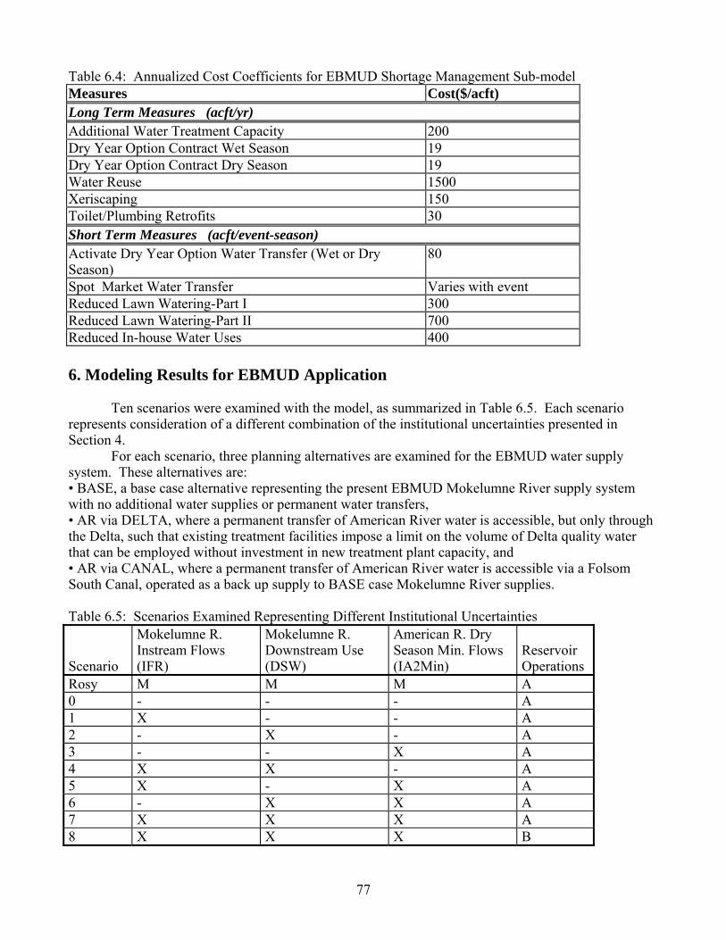
Table 6.4: Annualized Cost Coefficients for EBMUD Shortage Management Sub-model Measures Cost($/acft) Long Term Measures (acft/yr) Additional Water Treatment Capacity 200 Dry Year Option Contract Wet Season 19 Dry Year Option Contract Dry Season 19 Water Reuse 1500 Xeriscaping 150 Toilet/Plumbing Retrofits 30 Short Term Measures (acft/event-season) Activate Dry Year Option Water Transfer (Wet or Dry Season)

80

Spot Market Water Transfer Varies with event Reduced Lawn Watering-Part I 300 Reduced Lawn Watering-Part II 700 Reduced In-house Water Uses 400 6. Modeling Results for EBMUD Application Ten scenarios were examined with the model, as summarized in Table 6.5. Each scenario represents consideration of a different combination of the institutional uncertainties presented in Section 4. For each scenario, three planning alternatives are examined for the EBMUD water supply system. These alternatives are: • BASE, a base case alternative representing the present EBMUD Mokelumne River supply system with no additional water supplies or permanent water transfers, • AR via DELTA, where a permanent transfer of American River water is accessible, but only through the Delta, such that existing treatment facilities impose a limit on the volume of Delta quality water that can be employed without investment in new treatment plant capacity, and • AR via CANAL, where a permanent transfer of American River water is accessible via a Folsom South Canal, operated as a back up supply to BASE case Mokelumne River supplies. Table 6.5: Scenarios Examined Representing Different Institutional Uncertainties Scenario

Mokelumne R. Instream Flows (IFR)

Mokelumne R. Downstream Use (DSW)

American R. Dry Season Min. Flows (IA2Min)

Reservoir Operations

Rosy M M M A 0 - - - A 1 X - - A 2 - X - A 3 - - X A 4 X X - A 5 X - X A 6 - X X A 7 X X X A 8 X X X B

77

A - Base case variable carryover storage rule derived for Scenario 0 B - Fixed carryover storage rule M - Minimum value from Table 6.3 assumed deterministically X - Probability distribution used, otherwise "most likely" (i.e. expected value of probability distribution in Table 6.3) value was used Cost results from all scenarios of the two permanent American River water transfer alternatives represent the sum of supply system net operating and maintenance costs over BASE case plus the minimum expected value cost of shortage management. For the BASE case, the cost results represent only the minimum expected value cost of shortage management as the BASE case supply system is the reference for supply yield operating and maintenance costs. Under each scenario where institutional uncertainties are examined, the integrated model is run for each of the three alternatives, following the approach laid out in Figure 5.4, to produce a cumulative probability distribution of water supply system annual costs for each alternative. Figure 6.5 shows a typical plot of these results for one scenario (#7), in which the cumulative distribution curve is used to display probabilistic costs for each alternative. These probability distributions of annual cost are summarized by their expected value costs in Table 6.6. This allows rapid and rigorous assessment and comparison of alternatives and scenarios based on a single value measure of cost (Park and Sharp-Bette, 1990). The range of the annual cost distributions for each scenario appears in Table 6.7. For all cases, connection with the American River via a Canal had the lowest expected value cost, including both supply system operation and demand management and water transfer costs. The AR via Canal costs in all scenarios do not include additional capital investment costs required to build the canal structures needed to physically convey and transfer this water to EBMUD. Figure 6.5: Cumulative Distribution of Annual Costs for Scenario 7, for All Institutional Uncertainties

78

0.0

0.1

0.2

0.3

0.4

0.5

0.6

0.7

0.8

0.9

1.0

0 1 2 3 4 5 6 7 8 9 10 11 12 13 14 15 16 17 18 19 20Annual Cost of Alternative ($M)

BASE 7.95 $M

AR via DELTA7.05 $M

AR via CANAL3.29 $M

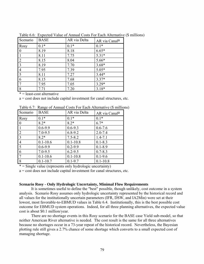
Table 6.6: Expected Value of Annual Costs For Each Alternative ($ millions) Scenario BASE AR via Delta AR via Canala Rosy 0.1* 0.1* 0.1* 0 8.19 8.18 6.65* 1 8.11 7.75 5.31* 2 8.15 8.04 5.66* 3 8.19 7.70 3.68* 4 7.95 7.39 5.05* 5 8.11 7.27 3.44* 6 8.15 7.68 3.37* 7 7.95 7.05 3.29* 8 7.71 7.20 3.18* * = least-cost alternative a = cost does not include capital investment for canal structures, etc. Table 6.7: Range of Annual Costs For Each Alternative ($ millions) Scenario BASE AR via Delta AR via Canala Rosy 0.1* 0.1* 0.1* 0 8.2* 8.2* 6.7* 1 0.6-9.9 0.6-9.3 0.6-7.6 2 7.0-9.5 6.8-9.2 2.0-7.4 3 8.2* 7.5-8.2 1.4-7.1 4 0.1-10.6 0.1-10.8 0.1-8.3 5 0.6-9.9 0.2-9.9 0.1-8.9 6 7.0-9.5 6.2-9.5 0.7-8.3 7 0.1-10.6 0.1-10.8 0.1-9.6 8 0.1-10.7 0.1-9.7 0.1-10.8 * = Single value (represents only hydrologic uncertainty) a = cost does not include capital investment for canal structures, etc. Scenario Rosy - Only Hydrologic Uncertainty, Minimal Flow Requirements It is sometimes useful to define the "best" possible, though unlikely, cost outcome in a system analysis. Scenario Rosy assumes only hydrologic uncertainty represented by the historical record and all values for the institutionally uncertain parameters (IFR, DSW, and IA2Min) were set at their lowest, most favorable-to-EBMUD values in Table 6.4. Institutionally, this is the best possible cost outcome for EBMUD system operations. Indeed, for all three planning alternatives, the expected value cost is about $0.1 million/year. There are no shortage events in this Rosy scenario for the BASE case Yield sub-model, so that neither American River alternative is needed. The cost result is the same for all three alternatives because no shortages occur in a 73-year repeat of the historical record. Nevertheless, the Bayesian plotting rule still gives a 2.7% chance of some shortage which converts to a small expected cost of managing shortage.

79

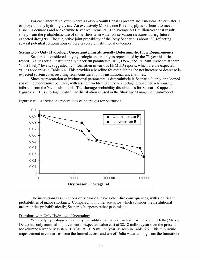
For each alternative, even where a Folsom South Canal is present, no American River water is employed in any hydrologic year. An exclusively Mokelumne River supply is sufficient to meet EBMUD demands and Mokelumne River requirements. The average $0.1 million/year cost results solely from the probabilistic use of some short-term water conservation measures during future expected droughts. The subjective joint probability of the Rosy Scenario is about 1%, reflecting several potential combinations of very favorable institutional outcomes. Scenario 0 - Only Hydrologic Uncertainty, Institutionally Deterministic Flow Requirements Scenario 0 considered only hydrologic uncertainty as represented by the 73-year historical record. Values for all institutionally uncertain parameters (IFR, DSW, and IA2Min) were set at their "most likely" levels, suggested by information in various EBMUD reports, which are the expected values appearing in Table 6.4. This provides a baseline for establishing the net increase or decrease in expected system costs resulting from consideration of institutional uncertainties. Since representation of institutional parameters is deterministic in Scenario 0, only one looped run of the model must be made, with a single yield-reliability or shortage probability relationship inferred from the Yield sub-model. The shortage probability distributions for Scenario 0 appears in Figure 6.6. This shortage probability distribution is used in the Shortage Management sub-model. Figure 6.6: Exceedence Probabilities of Shortages for Scenario 0

00.010.02

0.030.040.050.060.07

0.080.090.1

0 50000 100000 150000Dry Season Shortage (af)

with American R.no American R.

The institutional assumptions of Scenario 0 have rather dire consequences, with significant probabilities of major shortages. Compared with other scenarios which consider the institutional uncertainties probabilistically, Scenario 0 appears rather pessimistic. Decisions with Only Hydrologic Uncertainty With only hydrologic uncertainty, the addition of American River water via the Delta (AR via Delta) has only minimal improvement in expected value cost at $8.18 million/year over the present Mokelumne River only system (BASE) at $8.19 million/year, as seen in Table 6.6. This minuscule improvement in cost arises from the limited access and use of Delta water arising from the limitations

80

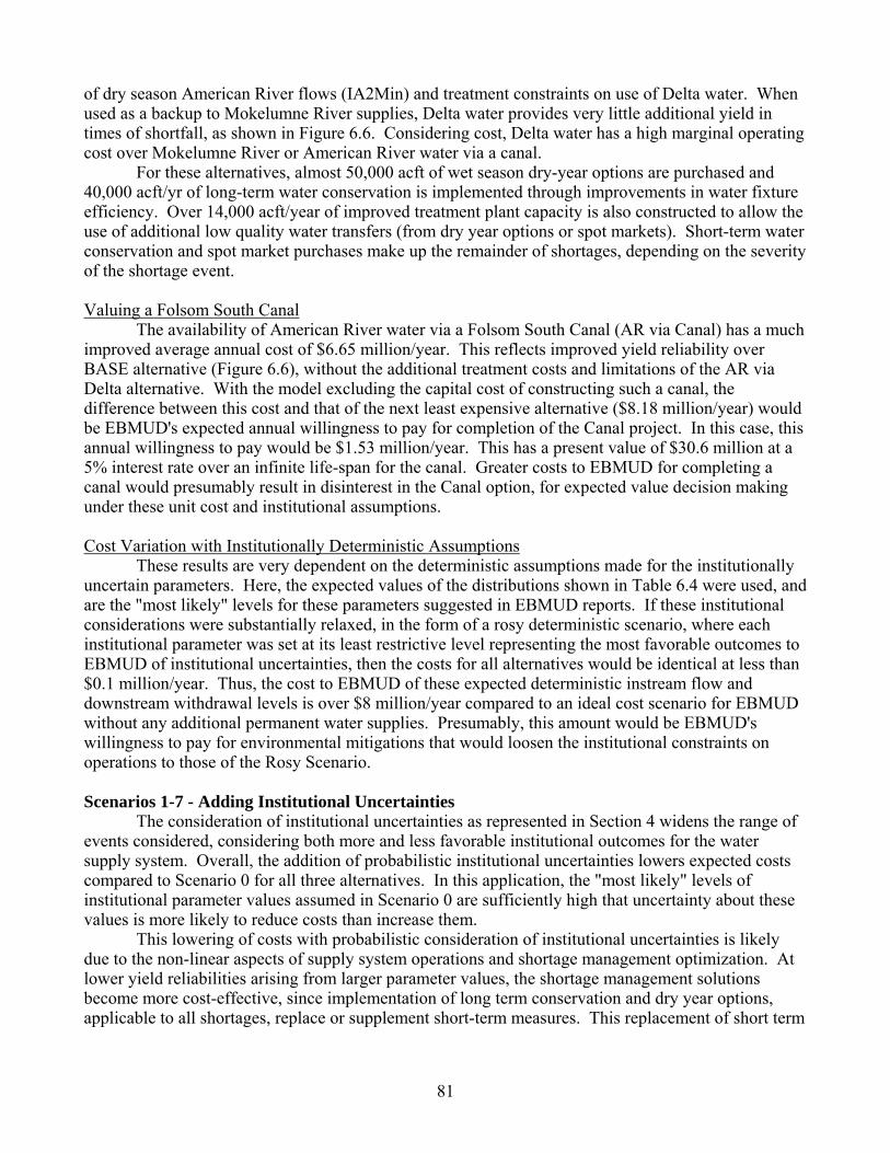
of dry season American River flows (IA2Min) and treatment constraints on use of Delta water. When used as a backup to Mokelumne River supplies, Delta water provides very little additional yield in times of shortfall, as shown in Figure 6.6. Considering cost, Delta water has a high marginal operating cost over Mokelumne River or American River water via a canal. For these alternatives, almost 50,000 acft of wet season dry-year options are purchased and 40,000 acft/yr of long-term water conservation is implemented through improvements in water fixture efficiency. Over 14,000 acft/year of improved treatment plant capacity is also constructed to allow the use of additional low quality water transfers (from dry year options or spot markets). Short-term water conservation and spot market purchases make up the remainder of shortages, depending on the severity of the shortage event. Valuing a Folsom South Canal The availability of American River water via a Folsom South Canal (AR via Canal) has a much improved average annual cost of $6.65 million/year. This reflects improved yield reliability over BASE alternative (Figure 6.6), without the additional treatment costs and limitations of the AR via Delta alternative. With the model excluding the capital cost of constructing such a canal, the difference between this cost and that of the next least expensive alternative ($8.18 million/year) would be EBMUD's expected annual willingness to pay for completion of the Canal project. In this case, this annual willingness to pay would be $1.53 million/year. This has a present value of $30.6 million at a 5% interest rate over an infinite life-span for the canal. Greater costs to EBMUD for completing a canal would presumably result in disinterest in the Canal option, for expected value decision making under these unit cost and institutional assumptions. Cost Variation with Institutionally Deterministic Assumptions These results are very dependent on the deterministic assumptions made for the institutionally uncertain parameters. Here, the expected values of the distributions shown in Table 6.4 were used, and are the "most likely" levels for these parameters suggested in EBMUD reports. If these institutional considerations were substantially relaxed, in the form of a rosy deterministic scenario, where each institutional parameter was set at its least restrictive level representing the most favorable outcomes to EBMUD of institutional uncertainties, then the costs for all alternatives would be identical at less than $0.1 million/year. Thus, the cost to EBMUD of these expected deterministic instream flow and downstream withdrawal levels is over $8 million/year compared to an ideal cost scenario for EBMUD without any additional permanent water supplies. Presumably, this amount would be EBMUD's willingness to pay for environmental mitigations that would loosen the institutional constraints on operations to those of the Rosy Scenario. Scenarios 1-7 - Adding Institutional Uncertainties The consideration of institutional uncertainties as represented in Section 4 widens the range of events considered, considering both more and less favorable institutional outcomes for the water supply system. Overall, the addition of probabilistic institutional uncertainties lowers expected costs compared to Scenario 0 for all three alternatives. In this application, the "most likely" levels of institutional parameter values assumed in Scenario 0 are sufficiently high that uncertainty about these values is more likely to reduce costs than increase them. This lowering of costs with probabilistic consideration of institutional uncertainties is likely due to the non-linear aspects of supply system operations and shortage management optimization. At lower yield reliabilities arising from larger parameter values, the shortage management solutions become more cost-effective, since implementation of long term conservation and dry year options, applicable to all shortages, replace or supplement short-term measures. This replacement of short term

81

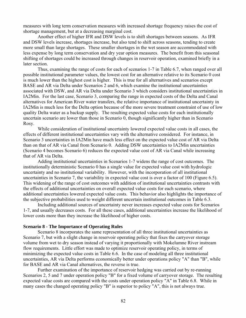
measures with long term conservation measures with increased shortage frequency raises the cost of shortage management, but at a decreasing marginal cost. Another effect of higher IFR and DSW levels is to shift shortages between seasons. As IFR and DSW levels increase, shortages increase, but also tend to shift across seasons, tending to create more small than large shortages. These smaller shortages in the wet season are accommodated with less expense by long term conservation and dry year option measures. The benefit from this seasonal shifting of shortages could be increased through changes in reservoir operation, examined briefly in a later section. Thus, examining the range of costs for each of scenarios 1-7 in Table 6.7, when ranged over all possible institutional parameter values, the lowest cost for an alternative relative to its Scenario 0 cost is much lower than the highest cost is higher. This is true for all alternatives and scenarios except BASE and AR via Delta under Scenarios 2 and 6, which examine the institutional uncertainties associated with DSW, and AR via Delta under Scenario 3 which considers institutional uncertainties in IA2Min. For the last case, Scenario 3, comparing the range in expected costs of the Delta and Canal alternatives for American River water transfers, the relative importance of institutional uncertainty in IA2Min is much less for the Delta option because of the more severe treatment constraint of use of low quality Delta water as a backup supply. The resulting expected value costs for each institutionally uncertain scenario are lower than those in Scenario 0, though significantly higher than in Scenario Rosy. While consideration of institutional uncertainty lowered expected value costs in all cases, the effects of different institutional uncertainties vary with the alternative considered. For instance, in Scenario 3 uncertainties in IA2Min have much less effect on the expected value cost of AR via Delta than on that of AR via Canal from Scenario 0. Adding DSW uncertainties to IA2Min uncertainties (Scenario 4 becomes Scenario 6) reduces the expected value cost of AR via Canal while increasing that of AR via Delta. Adding institutional uncertainties in Scenarios 1-7 widens the range of cost outcomes. The institutionally deterministic Scenario 0 has a single value for expected value cost with hydrologic uncertainty and no institutional variability. However, with the incorporation of all institutional uncertainties in Scenario 7, the variability in expected value cost is over a factor of 100 (Figure 6.5). This widening of the range of cost outcomes with addition of institutional uncertainties contrasts with the effects of additional uncertainties on overall expected value costs for each scenario, where additional uncertainties lowered expected value costs. This behavior also highlights the importance of the subjective probabilities used to weight different uncertain institutional outcomes in Table 6.3. Including additional sources of uncertainty never increases expected value costs for Scenarios 1-7, and usually decreases costs. For all these cases, additional uncertainties increase the likelihood of lower costs more than they increase the likelihood of higher costs. Scenario 8 - The Importance of Operating Rules Scenario 8 incorporates the same representation of all three institutional uncertainties as Scenario 7, but with a slight change in reservoir operating policy that fixes the carryover storage volume from wet to dry season instead of varying it proportionally with Mokelumne River instream flow requirements. Little effort was made to optimize reservoir operating policy, in terms of minimizing the expected value costs in Table 6.6. In the case of modeling all three institutional uncertainties, AR via Delta performs economically better under operations policy "A" than "B", while for BASE and AR via Canal alternatives, the reverse is true. Further examination of the importance of reservoir hedging was carried out by re-running Scenarios 2, 5 and 7 under operation policy "B" for a fixed volume of carryover storage. The resulting expected value costs are compared with the costs under operation policy "A" in Table 6.8. While in many cases the changed operating policy "B" is superior to policy "A", this is not always true.

82

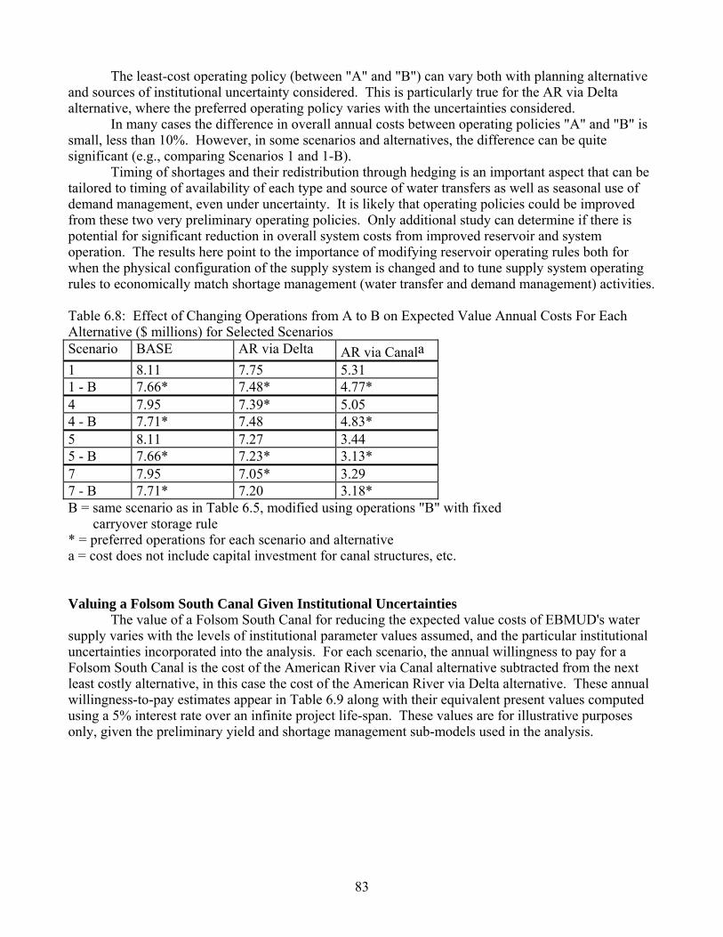
The least-cost operating policy (between "A" and "B") can vary both with planning alternative and sources of institutional uncertainty considered. This is particularly true for the AR via Delta alternative, where the preferred operating policy varies with the uncertainties considered. In many cases the difference in overall annual costs between operating policies "A" and "B" is small, less than 10%. However, in some scenarios and alternatives, the difference can be quite significant (e.g., comparing Scenarios 1 and 1-B). Timing of shortages and their redistribution through hedging is an important aspect that can be tailored to timing of availability of each type and source of water transfers as well as seasonal use of demand management, even under uncertainty. It is likely that operating policies could be improved from these two very preliminary operating policies. Only additional study can determine if there is potential for significant reduction in overall system costs from improved reservoir and system operation. The results here point to the importance of modifying reservoir operating rules both for when the physical configuration of the supply system is changed and to tune supply system operating rules to economically match shortage management (water transfer and demand management) activities. Table 6.8: Effect of Changing Operations from A to B on Expected Value Annual Costs For Each Alternative ($ millions) for Selected Scenarios Scenario BASE AR via Delta AR via Canala 1 8.11 7.75 5.31 1 - B 7.66* 7.48* 4.77* 4 7.95 7.39* 5.05 4 - B 7.71* 7.48 4.83* 5 8.11 7.27 3.44 5 - B 7.66* 7.23* 3.13* 7 7.95 7.05* 3.29 7 - B 7.71* 7.20 3.18* B = same scenario as in Table 6.5, modified using operations "B" with fixed carryover storage rule * = preferred operations for each scenario and alternative a = cost does not include capital investment for canal structures, etc. Valuing a Folsom South Canal Given Institutional Uncertainties The value of a Folsom South Canal for reducing the expected value costs of EBMUD's water supply varies with the levels of institutional parameter values assumed, and the particular institutional uncertainties incorporated into the analysis. For each scenario, the annual willingness to pay for a Folsom South Canal is the cost of the American River via Canal alternative subtracted from the next least costly alternative, in this case the cost of the American River via Delta alternative. These annual willingness-to-pay estimates appear in Table 6.9 along with their equivalent present values computed using a 5% interest rate over an infinite project life-span. These values are for illustrative purposes only, given the preliminary yield and shortage management sub-models used in the analysis.

83

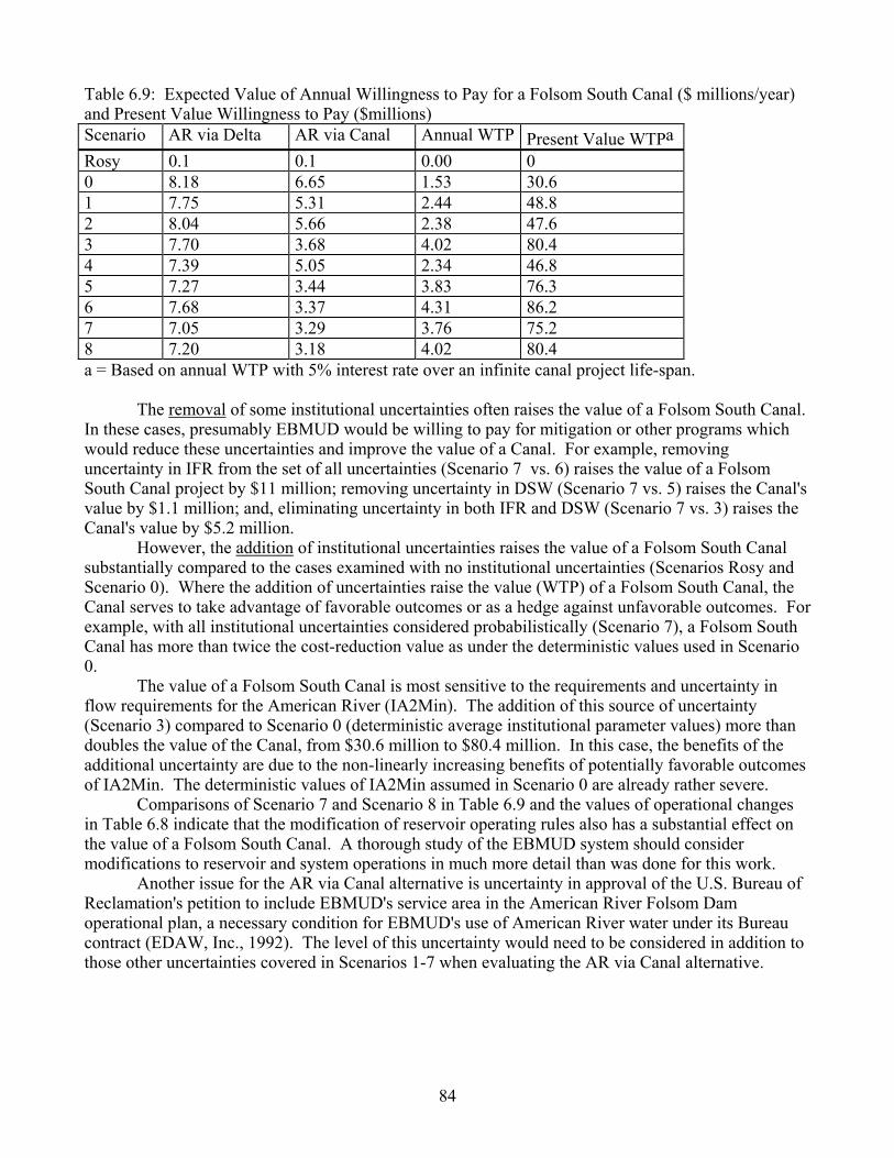
Table 6.9: Expected Value of Annual Willingness to Pay for a Folsom South Canal ($ millions/year) and Present Value Willingness to Pay ($millions) Scenario AR via Delta AR via Canal Annual WTP Present Value WTPa Rosy 0.1 0.1 0.00 0 0 8.18 6.65 1.53 30.6 1 7.75 5.31 2.44 48.8 2 8.04 5.66 2.38 47.6 3 7.70 3.68 4.02 80.4 4 7.39 5.05 2.34 46.8 5 7.27 3.44 3.83 76.3 6 7.68 3.37 4.31 86.2 7 7.05 3.29 3.76 75.2 8 7.20 3.18 4.02 80.4 a = Based on annual WTP with 5% interest rate over an infinite canal project life-span. The removal of some institutional uncertainties often raises the value of a Folsom South Canal. In these cases, presumably EBMUD would be willing to pay for mitigation or other programs which would reduce these uncertainties and improve the value of a Canal. For example, removing uncertainty in IFR from the set of all uncertainties (Scenario 7 vs. 6) raises the value of a Folsom South Canal project by $11 million; removing uncertainty in DSW (Scenario 7 vs. 5) raises the Canal's value by $1.1 million; and, eliminating uncertainty in both IFR and DSW (Scenario 7 vs. 3) raises the Canal's value by $5.2 million. However, the addition of institutional uncertainties raises the value of a Folsom South Canal substantially compared to the cases examined with no institutional uncertainties (Scenarios Rosy and Scenario 0). Where the addition of uncertainties raise the value (WTP) of a Folsom South Canal, the Canal serves to take advantage of favorable outcomes or as a hedge against unfavorable outcomes. For example, with all institutional uncertainties considered probabilistically (Scenario 7), a Folsom South Canal has more than twice the cost-reduction value as under the deterministic values used in Scenario 0. The value of a Folsom South Canal is most sensitive to the requirements and uncertainty in flow requirements for the American River (IA2Min). The addition of this source of uncertainty (Scenario 3) compared to Scenario 0 (deterministic average institutional parameter values) more than doubles the value of the Canal, from $30.6 million to $80.4 million. In this case, the benefits of the additional uncertainty are due to the non-linearly increasing benefits of potentially favorable outcomes of IA2Min. The deterministic values of IA2Min assumed in Scenario 0 are already rather severe. Comparisons of Scenario 7 and Scenario 8 in Table 6.9 and the values of operational changes in Table 6.8 indicate that the modification of reservoir operating rules also has a substantial effect on the value of a Folsom South Canal. A thorough study of the EBMUD system should consider modifications to reservoir and system operations in much more detail than was done for this work. Another issue for the AR via Canal alternative is uncertainty in approval of the U.S. Bureau of Reclamation's petition to include EBMUD's service area in the American River Folsom Dam operational plan, a necessary condition for EBMUD's use of American River water under its Bureau contract (EDAW, Inc., 1992). The level of this uncertainty would need to be considered in addition to those other uncertainties covered in Scenarios 1-7 when evaluating the AR via Canal alternative.

84

7. Some Methodological Comments Several methodological points and limitations can now be made, comparing this limited application of the modeling approach to the EBMUD system to how it might be applied for a real decision-making application. 1. The subjective institutional uncertainties involved in integrated water supply planning are obviously important. The approach presented allows us to assess the importance of these uncertainties and the implications of various necessarily subjective estimates of these uncertainties. Moreover, the approach allows us to suggest least-cost planning measures for dealing with these uncertainties. 2. The integration of reservoir/system operating rules is an essential part of least-cost planning for water supply systems. The operating rules for the yield system should be tuned to the demand management, water transfers, and other shortage management measures available. The approach presented here illustrates this point and provides a comprehensive technical methodology for such system integration. Ideally, for each combination of levels for uncertain institutional parameters, the operation of the yield system would be jointly optimized with available shortage management measures to minimize expected value cost. 3. For the case of EBMUD, the operations of the reservoir system and water sources has a great impact on the water transfers, demand management measures, costs, and reliabilities of the integrated system. The American River permanent water transfer alternatives were made far less attractive in the Yield sub-model by requiring that this source act only as a back-up to Mokelumne River supplies when they were inadequate. An actual study should examine a much wider range of operating rule alternatives than could be examined here. 4. Some activities in the model that are now artificially separated by model structure should perhaps be linked. For example, water quality treatment tradeoffs for involving different water transfer types might be linked. Water quality issues for permanent transfers in the Yield sub-model currently are not integrated with water treatment issues related to shortage management transfer decisions. 5. Discretization levels of shortage events used in the Shortage Management sub-model can be very important when evaluating performance of alternatives. Ideally, a much finer discretization would reduce the effects of shortage discretization on jumps or discontinuities in overall costs as uncertain parameters change. Discretization was limited in this case primarily by the need to retain the linear program-based Shortage Management sub-model within the limits of the spreadsheet optimizing software. 6. Discretization of levels of institutional parameters can have great importance for overall results and affect their probability levels as well. Here a fairly coarse, five point, discretization was used. While such a coarse discretization can result in jumps in model results, a finer discretization is costly in two ways. First, finer discretization of institutional parameter values can greatly increase the number of Yield and Shortage Management sub-model runs required. In this case, we considered three institutionally uncertain parameters, each having five possible values; this required a total of 53 (= 125) runs of the combined Yield and Shortage Management sub-models. Had the discretization been made finer at 10 levels per parameter, examination of three such uncertain parameters would require 103 (= 1,000) combined-model runs. A second, and perhaps ultimately greater problem from fine discretization of institutional uncertainties is assessing the subjective probability values for such distributions. A finer discretization might give undue confidence in these distributions and probably would entail more human effort and daring to estimate. 7. Parameter values are undoubtedly correlated through shared institutional issues. The minimum instream flow requirements IFR and IA2Min are likely to be correlated as a result of common agency, judicial, and political decision making. It is difficult and awkward to establish a

85

necessarily subjective correlation between these outcomes. However, it would be possible to extend this technical planning method to examine the importance of prospective correlations. 8. This analysis was relatively easily and rapidly accomplished using speadsheet software. The incorporation of optimization algorithms within the spreadsheet software greatly facilitated the modeling. The primary disadvantage of using spreadsheet software was the limited size of the Shortage Management sub-model which could be solved and the resulting limitation of a two-season model. 8. Conclusions The following conclusions are suggested by this application of the methodology presented in Chapter 5 to a simplified case of the East Bay Municipal Utility District. 1. As demonstrated in this chapter, it is possible to represent institutional uncertainties for practical engineering studies of urban water supply by extending traditional yield-reliability studies. 2. The economic and decision-making implications of these uncertainties can further be examined by extending traditional yield-reliability studies to incorporate shortage management decisions and their costs. The feasibility of such studies was demonstrated in this chapter. 3. Least-cost engineering of urban water supply systems requires integrated modeling of water supply system operations, demand management, and water transfer measures. Least-cost planning requires that the yield portions of water supply systems be tuned to the water transfer and demand management measures adopted for the system. Conversely, the economics and effectiveness of various water transfer and demand management measures will be affected by the physical capabilities and operation of the water supply system, typically the subject of traditional water supply yield studies. Such integrated modeling was accomplished in this chapter. 4. The approach demonstrated in this chapter can also be used to assess the economic value to a utility of various improvements in physical infrastructure, such as reservoirs, aqueducts, and treatment plants, considering both hydrologic and institutional uncertainties. This was demonstrated here for the case of a Folsom South Canal. This willingness to pay approach can also be applied to estimating the economic value of particular resolutions or modifications of institutional or hydrologic uncertainties. 5. As the statistician G.E.P. Box once wrote (1979), "All models are wrong, but some are useful". This modeling approach for water supply problems has many obvious limitations. However, it should have uses for structuring the problem in a logical way, assessing the economic and performance implications of proposed actions, and suggesting promising combinations of supply and demand management measures for least-cost performance.

86

Chapter 7 Conclusions

1. Conclusions This report has four major conclusions. Many other and more specific conclusions appear at the end of each chapter. 1. It is technically possible to perform integrated economic-engineering studies of urban water supplies. The approach developed here extends common yield-reliability studies to:

a. integrate yield enhancement, demand management, and water transfer decisions, b. provide an economic and risk-based approach to planning, as opposed to an approach based

solely on yield, and c. examine explicitly institutional uncertainties inherent in urban water supply planning.

2. The proposed technical approach (summarized in Chapter 5) is practical for actual urban water supply problems.

a. Historical streamflows are used to estimate yield-reliability using common yield simulation models with an enhanced Bayesian interpretation of shortage and yield probability plotting positions.

b. A cost-minimizing shortage management model is used to integrate long and short term demand management and water transfer responses to shortages.

c. The approach is very feasible computationally; here, an entire analysis of the East Bay Municipal Utility District (EBMUD) system was performed with common spreadsheet software.

d. Little is required in the way of new data. 3. It is possible to examine the joint effects of multiple institutional and hydrologic uncertainties for urban water supply planning.

a. Institutional uncertainties are complex and interact in ways which are not always intuitive and which are too complex for simple analytical methods.

b. Modeling studies are needed to fully understand the implications of institutional uncertainties for urban water supply planning. Model analyses of the most worrisome uncertainties can be done without unrealistic amounts of effort. However, it is probably impossible to explicitly include all institutional uncertainties in a modeling analysis.

c. Least-cost planning and management decisions, and their overall cost, can vary with both institutional and hydrologic uncertainties.

d. System and reservoir operation and shortage management decisions must be made jointly to minimize total system cost under conditions of uncertainty.

e. The economic or cost consequences of various uncertainties can be estimated through the use of the modeling approach described in Chapter 5 and demonstrated in Chapter 6.

f. It is possible to estimate a utility's willingness-to-pay for infrastructure or mitigation efforts which modify uncertainty in institutional or hydrologic events.

4. Water transfers can be engineered to improve their contribution to urban water supplies.

a. To most economically and effectively serve urban water supplies, the various forms of water transfers should be engineered integrally with other water sources, demand management measures, and overall system operating rules.

87

b. Institutional uncertainty is important for the economical design and integration of water transfers for urban water supplies.

c. The method presented here explicitly integrates several forms of water transfers into urban water supply systems considering both hydrologic and institutional uncertainties.

2. Further Research Several extensions to this research are suggested, building on the technical approach developed in this study. 1. The approach presented here should be extended to improve the optimization of yield system operating rules when integrated with shortage management measures. Here, shortage management measures were chosen to minimize costs, given a set of reservoir operating rules. It would be useful to examine the optimization of reservoir operating rules, particularly hedging or carryover storage rules in the context of demand management and water transfer measures for responding to shortages. 2. The cost and availability uncertainties involved in the design of water transfers should be more explicitly addressed, particularly for dry year option and spot market transfers. 3. Regarding the development of Bayesian plotting positions, the possibility of varying priors with shortage level should be explored. 4. The model presented here of the EBMUD system involved a fairly coarse representation of shortage levels and various demand and water transfer measures. Examining the effects of using finer levels of discretization might be useful.

88

References Abramowitz, M. and I.A. Stegan (1965), Handbook of Mathematical Functions, Dover Publications,

N.Y., NY. Asano, T. and R.A. Mills (1990), “ Planning and Analysis for Water Reuse Projects”, American Water

Works Association Journal Vol. 82, pp. 38-47. Asano, T. and R.S. Madancy (1984), “ Water Reclamation Efforts in the United States”, Water Reuse ,

Ann Arbor Science, pp. 277-291. Bain, J.S., R.E. Caves, and J. Margolis (1966), Northern California's Water Industry, Resources for

the Future, The Johns Hopkins University Press, Baltimore, MD. Beecher, J.A. (1995), “Integrated Resource Planning Fundamentals”, American Water Works

Association Journal, Vol. 87 pp. 34-48. Box, G.E.P. and G.C. Tiao (1973), Bayesian Inference in Statistical Analysis, John Wiley and Sons,

Inc., N.Y. Brajer, V., A.L. Church, R. Cummings, and P. Farah (1989), "The Strengths and Weaknesses of Water

Markets as They Affect Water Scarcity and Sovereignty Interests in the West," Natural Resources Journal, Vol. 29, Spring, pp. 489-509.

Buras, N. (1963), "Conjunctive Operation of Dams and Aquifers," Proceedings of the American Society of Civil Engineers, Vol. 89, No. HY6, pp. 111-131.

Butcher, W.S., Y.Y. Haimes, W.A. Hall (1969), “Dynamic Programming for the Optimal Sequencing of Water Supply Projects”, Water Resources Research , Vol. 5, No. 6, pp. 1196-

California Department of Water Resources (1994), Urban Water Use in California, Bulletin No. 166-4, California Department of Water Resources, Sacramento, CA.

California Department of Water Resources (1991), Urban Drought Guidebook, Water Conservation Office, California Department of Water Resources, Sacramento, CA.

California Department of Water Resources (1983), Urban Water Use in California, Bulletin No. 166-3, California Department of Water Resources, Sacramento, CA.

Capen, C.H. (1975), "Real or Rash Regionalization," Journal of the American Water Works Association, Vol. 67, No. 10, pp. 588-590.

Chow, V.T. and N. Takase (1977), "Design Criteria for Hydrologic Extremes," Journal of the Hydraulics Division, ASCE, Vol. 103, No. HY4, April, pp.425-436.

Chung, I. and Helweg, O. (1985), “Modeling the California State Water Project”, Journal of Water Resources Planning and Management, Vol. 111, No. 1, pp. 82- 97.

Colby, B.G. (1990), "Transactions Costs and Efficiency in Western Water Allocation," American Journal of Agricultural Economics, December, pp. 1184-1192.

Colby, B.G., D.B. Brush, W.E. Martin, and T.C. Brown (1987), "Do water market prices appropriately measure water values?," Natural Resources Journal, Vol. 27, No. 3, pp. 617-652.

89

Cowan, M.S.; R.W. Cheney, and J.C. Addiego (1981), “Colorado River Simulation System, An Executive Summary”, U.S. Bureau of Reclamation, Engineering and Research Center, Denver, Colorado, October.

Cunnane, C. (1978), "Unbiased Plotting Positions - A Review," Journal of Hydrology, Vol. 37, pp. 205-222.

CUWA (1992a), Evaluating Urban Water Conservation Programs: A Procedures Manual, California Urban Water Agencies, Sacramento, CA.

CUWA (1992b), Survey of 1991 Demand Management Measures, California Urban Water Agencies, Sacramento, CA.

CUWA (1991), Survey of 1991 Drought Management Measures, California Urban Water Agencies, Sacramento, CA.

DWR (1992), The 1991 Drought Water Bank, California Department of Water Resources, Sacramento, CA, January.

Dziegielewski, B.; Mee, W.R. Jr.; Larson, K.R. (1992), “Developing a Long-Term Drought Plan for Phoenix”, American Water Works Association Journal, Vol. 84 pp. 46-51.

Dziegielewski, B. and J.E. Crews (1986), "Minimizing the Cost of Coping with Droughts: Springfield, Illinois," Journal of Water Resources Planning and Management, ASCE, Vol. 112, No. 4, October, pp. 419-438.

East Bay Municipal Utility District, (1991), Urban Water Management Plan , Oakland, CA, February. EDAW Inc., EBMUD Updated WSMP EIS/EIR, Preliminary Draft, Aug. 1992. Ellis, W.H. and C.T. DuMars (1978), "The Two-Tiered Market in Western Water," Nebraska Law

Review, Vol. 57, No. 2, pp. 333-367. Englehardt, J.D. and J.R. Lund (1992), "Information Theory in Risk Analysis,"Journal of

Environmental Engineering, ASCE, Vol. 118, No. 6, November-December, pp. 890-904. Enright, C. and J.R. Lund (1991), "Alternative Water District Organization: A Screening Level

Analysis," Journal of Water Resources Planning and Management, ASCE, Vol. 117, No. 1, pp. 86-107, January.

Epstein, E.S. (1985), "Statistical inference and prediction in climatology: A Bayesian approach," Meteorological Monographs, Vol. 20, No. 42, 199 pp.

Ford, David T (1990), “Reservoir Storage Reallocation Analysis with PC”, Journal of Water Resources Planning and Management, Vol. 116, No. 3, pp. 402-416.

Gray, Brian E. (1990), "Water Transfers in California: 1981-1989," in MacDonnell, Lawrence J.(Principal Investigator), The Water Transfer Process As A Management Option for Meeting Changing Water Demands, Volume II, USGS Grant Award No. 14-08-0001-G1538, Natural Resources Law Center, University of Colorado, Boulder.

Gray, Brian E. (1989), "A Primer on California Water Transfer Law," Arizona Law Review, Vol. 31, pp. 745-781.

Hashimoto, T., J.R. Stedinger, and D.P. Loucks (1981), "Reliability, resiliency, and vulnerability criteria for water resource system performance evaluation," Water Resources Research, Vol. 18, No. 1, pp. 14-20.

90

Hirsch, R.M. (1978), Risk Analyses for A Water-Supply System - Occoquan Reservoir, Fairfax and Prince William Counties, Virginia, Open File Report 78-452, U.S. Geological Survey, Reston, VA, also in Hydrologic Science Bulletin, Vol. 23, No. 4, pp. 475-505.

Hirsch, R.M. (1981), Estimating Probabilities of Reservoir Storage for the Upper Delaware River Basin, Open File Report 81-478, U.S. Geological Survey, Reston, VA.

Hoagland, R. (n.d.), "Long Range Planning Concepts for Managing Future Water Supply," California Department of Water Resources Briefing Paper, Planning Division, Sacramento, CA.

Hoagland, R. (1996). Appendix 2: Interim South Delta Program Economic Analysis, Draft Environmental Impact Report/Environmental Impact Statement (EIR/EIS), Interim South Delta Program, Volume II, California Department of Water Resources, Sacramento, CA.

Howard, R.A. (1988), "Uncertainty about probability: A decision analysis perspective," Risk Analysis, Vol. 8, No. 1, pp. 91-98.

Howe, C.W., J.K. Lazo, and K.R. Weber (1990), "The Economic Impacts of Agriculture-to-Urban Water Transfers on the Area of Origin: A Case Study of the Arkansas River Valley in Colorado," American Journal of Agricultural Economics, December, pp. 1200-1204.

Howe, C.W., D.R. Schurmeier, and W.D. Shaw, Jr. (1986), "Innovative Approaches to Water Allocation: The Potential for Water Markets," Water Resources Research, Vol. 22, No. 4, April, pp. 439-445.

Howitt, R., N. Moore, and R.T. Smith (1992), “A Retrospective on California’s 1991 Emergency Drought Water Bank”. March.

Hydrologic Engineering Center (1993), "Columbia River Reservoir System Analysis: Phase II," Technical Report No. PR-21, Hydrologic Engineering Center, U.S. Army Corps of Engineers, Davis, CA, December.

Jaynes, E.T. (1996), Probability Theory: The Logic of Science, Draft Book, http://omega.albany.edu:8008/JaynesBook.html.

Jaynes, E.T. (1968), "Prior Probabilities," IEEE Transactions on Systems Science and Cybernetics, Vol. SSC-4, No. 3, September, pp. 227-241.

JAWWA (1995), Journal of the American Water Works Association, issue devoted to integrated resource planning, Vol. 87, No. 6, June.

Jeffreys, H. (1961), Theory of Probability, Clarendon Press, Oxford, UK, 447pp. Jensen, M.R. and J.R. Lund, "WATSUP: A Simulation Model for Water Supply Costs and Reliability,"

project completion report to the California Department of Water Resources, Sacramento, CA, June, 1993.

Karpack, L.M. and Palmer, R.N. (1992), “Use of Interactive Simulation Environment for Evaluation of Water Supply Reliability”, Proceedings of the Water Resources Sessions at Water Forum ‘92, M. Karamouz ed., 144-149, ASCE New York, NY

Krzysztofowicz, R. (1983), "Why should a forecaster and a decision maker use Bayes Theorem," Water Resources Research, Vol. 19, No. 2, pp. 327-336.

Kuczera, G. and G. Diment (1988), “General Water Supply System Simulation Model: WASP”, Journal of Water Resources Planning and Management, Vol. 114, No. 4, pp. 365-382.

91

Leconte, R., T.C. Hughes, R. Narayanan (1987), “ Economic Efficiency and Investment Timing for Dual Water Systems”, Water Resources Research, Vol. 23, No. 10, pp 1807-1815.

Linsley, R.K., J.B. Franzini, D.L. Freyberg, and G. Tchobanoglous (1992), Water Resources Engineering, McGraw-Hill, Inc, N.Y.

Loucks, D.P., J.R. Stedinger, and D.A. Haith (1981), Water Resource Systems Planning and Analysis, Prentice-Hall, Englewood Cliffs, NJ.

Lougee, N.H. (1991), "Uncertainties in Planning Inter-Agency Water Supply Transfers," in J.L. Anderson (ed.), Water Resources Planning and Management and Urban Water Resources, ASCE, New York, pp. 601-604.

Lund, J.R. (1995), "Derived Estimation of Willingness-to-Pay to Avoid Probabilistic Shortage," Water Resources Research, Vol. 31, No. 5, May, pp. 1367-1372.

Lund, J.R.(1993), "Transaction Risk versus Transaction Costs in Water Transfers," Water Resources Research, Vol. 29, No. 9, pp. 3103-3107, September.

Lund, J.R. (1991), "Random Variables Versus Uncertain Values: Stochastic Modeling and Design," Journal of Water Resources Planning and Management, ASCE, Vol. 117, No. 2, pp. 179-194, March.

Lund, J.R. (1988a), "Metropolitan Water Market Development in Seattle, Washinton, 1887-1987," Journal of Water Resources Planning and Management, ASCE, Vol. 114, No. 2, March, pp. 223-240.

Lund, J.R. (1988b), "Regional Water Supply Development in South Sweden," Journal of Urban Planning and Development, ASCE, Vol. 114, No. 1, June, pp. 14-33.

Lund, J.R. (1987), "Evaluation and Scheduling of Water Conservation," Journal of Water Resources Planning and Management, ASCE, Vol. 113, No. 5, pp. 696-708.

Lund, J.R. and M. Israel (1995), “ Optimization of Transfers in Urban Water Supply Planning”, Journal of Water Resources Planning and Management, Vol. 121, No. 1, pp. 41-48.

Lund, J.R., M. Israel, and R. Kanazawa (1992), Recent California Water Transfers: Emerging Options in Water Management, Center for Environmental and Water Resources Engineering Report No. 92-2, Department of Civil and Environmental Engineering, University of California, Davis, CA, November.

Maass, A., et al. (1966), Design of Water Resource Systems, Harvard University Press, Cambridge, MA.

MacDonnell, L.J. (ed.) (1990), The Water Transfer Process As A Management Option for Meeting Changing Water Demands, Volume I, USGS Grant Award No. 14-08-0001-G1538, Natural Resources Law Center, University of Colorado, Boulder.

Mann, P.C. and D.M. Clark (1993), “Marginal-Cost Pricing: Its Role in Conservation”, AWWA Journal, Vol 85 pp. 71-78.

Martin, Q.W. (1987), “Optimal Daily Operation of Surface-Water System”, Journal of Water Resources Planning and Management, Vol. 113, No. 4, pp. 456-470.

Morin, Thomas L. and Esogbue, Augustine M. O. (1971), “Some Efficient Dynamic Programming Algorithms for the Optimal Sequencing and Scheduling of Water Supply Projects”, Water Resources Research, Vol. 7, No. 3, pp. 479-

92

Mays, L.W. and Y-K Tung (1992), Hydrosystems Engineering and Management, McGraw-Hill, New York, NY.

Milliman, J.W. (1959), "Water Law and Private Decision-Making: A Critique," Journal of Law and Economics, Vol. 2, October, pp. 41-63.

Moss, M.E., C.P. Pearson, and A.I. McKerchar (1994), "The Southern Oscillation index as a predictor of the probability of low streamflows in New Zealand," Water Resources Research, Vol. 30, No. 10, pp. 2717-2723, October.

National Research Council (1992), Water Transfers in the West: Efficiency, Equity, and the Environment, National Research Council, National Academy Press, Washington, D.C.

Ng, W.S. and G. Kuczera (1993), "Incorporating Demand Uncertainty in Water Supply Headworks Sinulation," Water Resources Research, Vol. 29, No. 2, February, pp. 469-477.

Nunn, S.C. and H.M. Ingram (1988), "Information, the Decision Forum, and Third-Party Effects in Water Transfers," Water Resources Research, Vol. 24, No. 4, April, pp. 473-480.

O'Brien, K.M. (1988), "Water Marketing in California," Pacific Law Journal, Vol. 19, No. 4, pp. 1165-1200.

Ocanas, Gerardo and Mays, Larry W. (1981), “Water Reuse Planning Models: Extensions and Applications”, Water Resources Research, Vol. 17, No. 5, pp. 1311-1327.

Palmer, R.N. and J.K. Holmes (1988), “Operational Guidance During Droughts: Expert System Approach”, Journal of Water Resources Planning and Management, Vol. 114, No. 6, pp. 647-666.

Park, C.S. and G.P. Sharp-Bette (1990), Advanced Engineering Economics, John Wiley & Sons, Inc., N.Y.

Pretto, P.B., F.H.S. Chiew, T.A. McMahon, R.M. Vogel, and J.R. Stedinger (1997), "The (mis)behavior of behavior analysis storage estimates," Water Resources Research, Vol. 33, No. 4, April, pp. 703-709.

Randall, D., M.H. Houck, and J.R. Wright (1990), “Drought Management of Existing Water Supply System”, Journal of Water Resources Planning and Management, Vol. 116, No. 1, pp. 1-20.

Reisner, M. and S. Bates, (1990), Overtapped Oasis: Reform or Revolution for Western Water, Island Press, Washington, D.C.

Rippl, W. (1883), "The Capacity of Storage Reservoirs for Water Supply," Proceedings of the Institution of Civil Engineers (London), Vol. 71, pp. 270-278.

Rubenstein, J. and L. Ortolano (1984), "Water Conservation and Capacity Expansion," Journal of Water Resources Planning and Management, ASCE, Vol. 110, No. 2, pp. 220-237.

Russell, C., D. Arey, and R. Kates (1970), Drought and Water Supply, The Johns Hopkins University Press, Baltimore, MD.

Salas, J.D., J.W. Delleur, V. Yevjevich, and W.L. Lane, (1988), Applied Modeling of Hydrologic Time Series, Water Resources Publications, Highlands Ranch, CO, 498 pp.

Saleth, R.M., J.B. Braden, and J.W. Eheart (1991), "Bargaining Rules for a Thin Spot Water Market," Land Economics, Vol. 67, No. 3, pp. 326-339.

Shih, J-S and C. ReVelle (1995), “ Water Supply Operations During Drought: A Discrete Hedging Rule”, European Journal of Operational Research , Vol. 82, pp. 163-175.

93

SWRCB (1988), "Order Denying Petition for Temporary Urgency Change," Order: WR 88-15, State Water Resources Control Board, Sacramento, CA.

Taha, H.A. (1992), Operations Research, Macmillan Publishing Co., N.Y., NY. Tribus, M. (1969), Rational Descriptions, Decision and Designs, Pergamon Press, N.Y., NY. Vaux, H.J., Jr. and R.E. Howitt (1984), "Managing Water Scarcity: an Evaluation of Interregional

Transfers," Water Resources Research, Vol. 20, No. 7, July, pp. 785-792. Vitruvius (1st. c. B.C.), The Ten Books of Architecture, trans, Dover Publications, Inc., N.Y., 1960. Vogel, R.M. and R.A. Bolognese (1995), "Storage-reliability-resilience-yield relations for over-year

water supply systems," Water Resources Research, Vol 31, No. 3, March, pp. 645-654. Vogel, R.M., N.M. Fennessey, and R.A. Bolognese (1995), "Storage-Reliability-Resilience-Yield

Relations for Northeastern States," Journal of Water Resources Planning and Management, Vol. 121, No. 5, pp. 365-374.

Weber, J.A. (1993), “Integrating Conservation Targets into Water Demand Projections”, AWWA Journal, Vol 85 pp. 63-70.

Wilchfort, O. and J.R. Lund, "Shortage Management Modeling for Urban Water Supply Systems," Journal of Water Resources Planning and Management, ASCE, Vol. 123, No. 4, July/August 1997.

Willis, R. and W. W-G. Yeh (1987), Groundwater Systems Planning and Management, Prentice-Hall, Englewood Cliffs, NJ.

Wurbs, R.A. (1993), “Reservoir-System Simulation and Optimization Models”, Journal of Water Resources Planning and Management, Vol. 119, No. 4, pp. 455-472.

Wurbs, R.A. (1991), “Optimization of Multiple-Purpose Reservoir System Operations: A Review of Modeling and Analysis Approaches”, Hydrologic Engineering Center, U.S. Army Corps of Engineers.

Yeh, W. W-G. (1985), "Reservoir Management and Operations Models: A State of the Art Review," Water Resources Research, Vol. 21, No. 12, December, pp. 1797-1818.

Zabell, S.L. (1989), "The rule of succession," Erkinntnis, Vol. 31, Nos.2-3, September, pp. 283-321.

94