integrated business and technical product reliability design
TRANSCRIPT

PROJECT REPORT
KOTEL 256
31.12.2008
INTEGRATED BUSINESS AND TECHNICAL PRODUCT RELIABILITY DESIGN
KOTEL 256 Page 2
FOREWORD
The traditional and still dominating method for product design is focused on optimising the technical performance of a product. The reason for this is simple, there does not exist easily available and comprehensive design method or tool to integrate the reliability and maintainability (R&M) considerations and effects in product design.
As more the companies’ management have experienced the meaning of Product’s R&M as competitive factors in their business, as more they have started to invest R&M engineering and development. This was also a starting point from where this project was launched.
The purpose of the project was to develop a design methodology that includes the interactions and links between the customer needs, the manufacturer business targets and the product R&M performance. This makes it possible to find and simulate in detail, which are the specific customer product R&M requirements and what influence the R&M performance has on the customer satisfaction. The method enables product R&M facts to be taken into account at business decision level.
This research project was carried out by Tampere University of Technology with co-operation University of Queensland, Australian. KOTEL ry was responsible for managing the project with the help of project steering group. The project was funded by TEKES, ABB Oy, Kone Oyj, MacGregor Oy and Wärtsilä Oyj.
On behalf of KOTEL ry I would like to thank all who have participated in this project.
Espoo 2008-12-31
KOTEL ry
Antti Turtola
KOTEL 256 Page 3
CONTENTS
1. INTRODUCTION ...................................................................................... 4
2. PROJECT ISSUES ANALYSIS ................................................................ 5
3. OBJECTIVES AND WORK PLAN .......................................................... 5
4. RESOURCES SCHEDULE ....................................................................... 6
5. RESULTS ................................................................................................... 7
APPENDIXES:
1. Publication
2. Master Thesis
3. Developed Models
4. Case-Studies: Companies Presentations
ABSTRACT

KOTEL 256 Page 4
1. INTRODUCTION
The customer expectations are today increasingly integrated as design requirements into the design process. However, the reliability and maintainability (R&M) aspects of the product are still today very poorly integrated into the design process. This is a problem today when both the customer expectations and the societal requirements are increasingly focusing more on R&M aspects instead of purely technical performance.
In the design methods used today it is very much the design engineer that is responsible for the product’s R&M engineering. How well this is in agreement with the customer expectations depends on how well the engineer knows the end user and how well the R&M requirements have been specified. Typical problems arise when either 1) such an R&M performance is promised to the customer that cannot be achieved or 2) achieving the promised performance becomes very expensive for the company.
A company that has a good control of the R&M performance of its products has a considerable competition advantage both in the case of consumer products and when negotiating about maintenance service contracts for large industrial systems.
One basis for this research project has been carried out by prof. Seppo Virtanen’s research team at Tampere University of Technology. Since 1996 eleven Finnish companies have participated in the research project which objective was to develop computer supported probabilistic based method for the design and development of the equipment’s reliability, safety and maintenance service.
The research project consists of three parts:
1) Modelling and analysis of causes and consequences of failures, 2) Specification and allocation of reliability, availability and maintenance cost requirements, and 3) Simulation and calculation of reliability performance and maintenance costs.
Based on the experience, and with the help of the methods, it is possible to find out those problem areas during the design stage, which can reduce product R&M, increase product life cycle costs and delay product development.
Professor D.N.P. Murthy from the University of Queensland in Australia is one of the leading experts and scientists in reliability engineering in the world. He has published a great number of scientific papers, books and carried out industrial consultancy in many countries in different parts of the world. He has recently developed together with Ostreas and Rausand from Norwegian University of Science and Technology in Trondheim a new method called “Reliability Performance and Specifications in New Product Development". The novel feature of this is focusing on the front end in the product development process. This new approach as well as the large experience of professor Murthy was benefited in this research project.

KOTEL 256 Page 5
2. PROJECT ISSUES ANALYSIS
In the project preparation phase seven research issues were analyzed and ranked according to the industrial companies (Kone, Wärtsilä, ABB, Nokia and Metso) point of view. A summary of the study is below.
Issue No Integrated Business and Technical Product Reliability Design (BRED)The issues importance from BRED project point of view
6 How to include the customer view into the reliability of a product? Transferring customer needs to product roadmaps / top management strategy deployment
4 Need to formulate reliability parameters on terms of cash > profit. The LCC perspective 0.56
2 Simple tool to make reliability facts visible for top management is needed
3 A structure and procedure forming basis for making warranty strategy decisions and maintenance contracts / extended warranty is needed 0.14
5 How to get good (=reliable) data for the reliability calculations/estimations 0.14
7 How to include the uncertainty of middlemen (between supplier and end user) and small subcontractors in the reliability estimations 0.09
1 Small cheap components cause much trouble - time between stoppages important 0.07
0.70
3. OBJECTIVES AND WORK PLAN
The objective of the project was to develop a design methodology that includes the interactions and links between the customer needs, the manufacturer business targets and the product reliability and maintenance performance. This makes it possible to find and simulate in detail, which are the specific customer product R&M requirements and what influence the R&M performance has on the customer satisfaction. In addition the method enables to assure at different phases of the design process that the promised R&M performance can be delivered to the customer in accordance with the business expectations of the top management. Thus the method enables product R&M facts to be taken into account at business decision level.
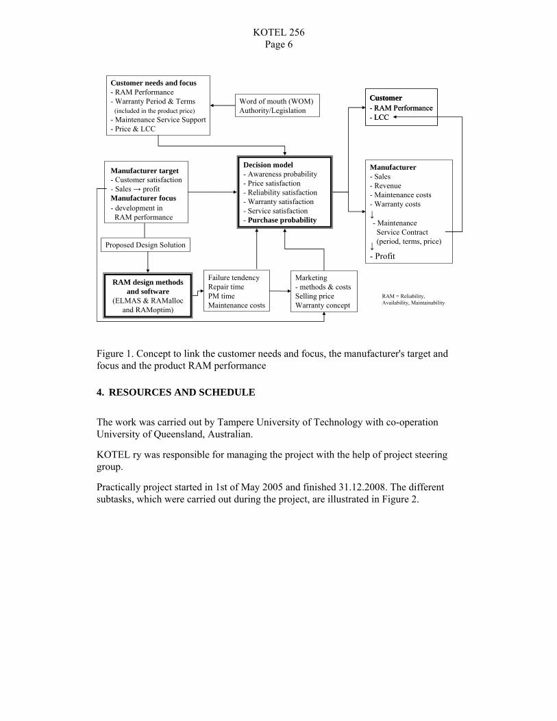
The work includes two parts: I) the development of “Decision model” and its integration to the developed “RAM design methods and software” (see Figure 1) and II) in parallel its implementation to four industrial cases. The “Decision model” consists of a holistic business-reliability structure which includes elements such as: a tool for making R&M facts visible for business level decisions and a tool for including the customer view into the R&M of the product. The experience from the industrial cases will during the process directly be used in the further development of the generic model.
KOTEL 256 Page 6
Figure 1. Concept to link the customer needs and focus, the manufacturer's target and focus and the product RAM performance
4. RESOURCES AND SCHEDULE
The work was carried out by Tampere University of Technology with co-operation University of Queensland, Australian.
KOTEL ry was responsible for managing the project with the help of project steering group.
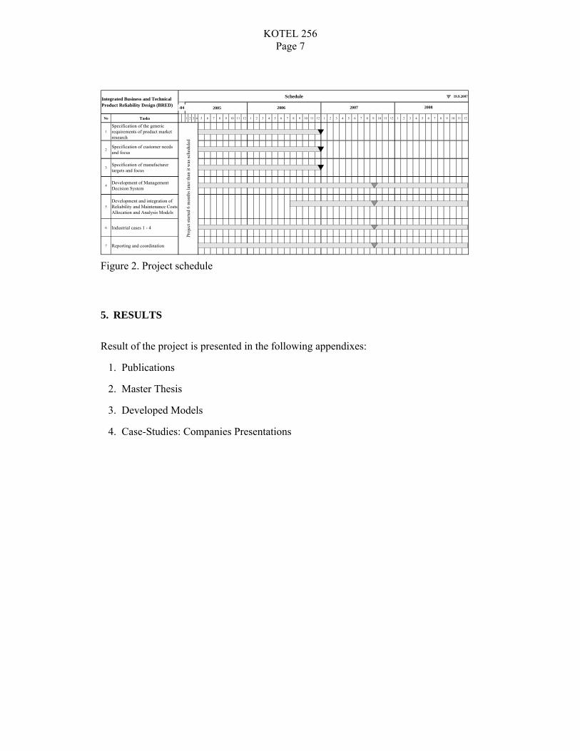
Practically project started in 1st of May 2005 and finished 31.12.2008. The different subtasks, which were carried out during the project, are illustrated in Figure 2.
Decision model- Awareness probability- Price satisfaction- Reliability satisfaction- Warranty satisfaction- Service satisfaction- Purchase probability
- Customer satisfaction- Sales → profitManufacturer focus
Customer needs and focus- RAM Performance- Warranty Period & Terms
(included in the product price)- Maintenance Service Support- Price & LCC
Failure tendencyRepair timePM timeMaintenance costs
Marketing - methods & costs Selling priceWarranty concept
Word of mouth (WOM) Authority/Legislation
- development in RAM performance
Manufacturer target
RAM design methods and software
(ELMAS & RAMallocand RAMoptim)
Manufacturer- Sales- Revenue- Maintenance costs- Warranty costs↓
↓- Profit
- RAM Performance- LCC
Customer- RAM Performance- LCC
Customer
- Maintenance Service Contract (period, terms, price)Proposed Design Solution
RAM = Reliability, Availability, Maintainability
KOTEL 256 Page 7
Figure 2. Project schedule
5. RESULTS
Result of the project is presented in the following appendixes:
1. Publications
2. Master Thesis
3. Developed Models
4. Case-Studies: Companies Presentations
Integrated Business and Technical Schedule 19.9.2007
Product Reliability Design (BRED)
No Tasks 1 2 3 4 5 6 7 8 9 10 11 12 1 2 3 4 5 6 7 8 9 10 11 12 1 2 3 4 5 6 7 8 9 10 11 12 1 2 3 4 5 6 7 8 9 10 11 12
1Specification of the generic requirements of product market research
2Specification of customer needs and focus
3Specification of manufacturer targets and focus
4Development of Management Decision System
5Development and integration of Reliability and Maintenance Costs Allocation and Analysis Models
6 Industrial cases 1 - 4
7 Reporting and coordination
Proj
ect s
tarte
d 6
mon
ths l
ater
than
it w
as sc
hedu
led
-04 2005 2006 2007 2008
KOTEL 256
Total number of pages in Appendix 14
APPENDIX 1
PUBLICATIONS
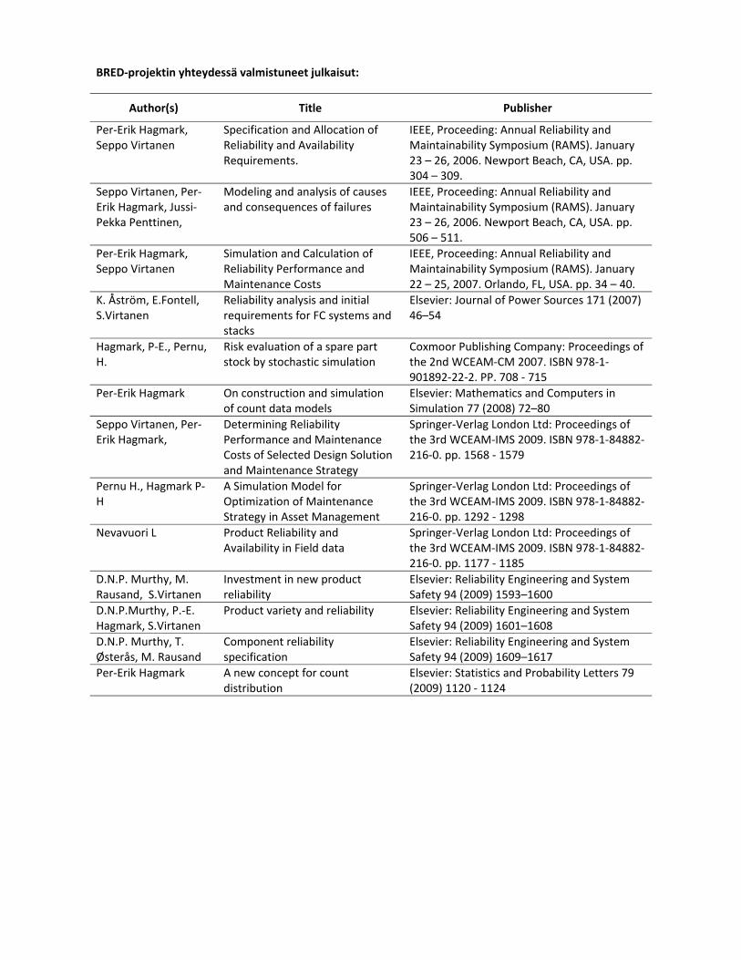
BRED‐projektin yhteydessä valmistuneet julkaisut:
Author(s) Title Publisher
Per‐Erik Hagmark, Seppo Virtanen
Specification and Allocation of Reliability and Availability Requirements.
IEEE, Proceeding: Annual Reliability and Maintainability Symposium (RAMS). January 23 – 26, 2006. Newport Beach, CA, USA. pp. 304 – 309.
Seppo Virtanen, Per‐Erik Hagmark, Jussi‐Pekka Penttinen,
Modeling and analysis of causes and consequences of failures
IEEE, Proceeding: Annual Reliability and Maintainability Symposium (RAMS). January 23 – 26, 2006. Newport Beach, CA, USA. pp. 506 – 511.
Per‐Erik Hagmark, Seppo Virtanen
Simulation and Calculation of Reliability Performance and Maintenance Costs
IEEE, Proceeding: Annual Reliability and Maintainability Symposium (RAMS). January 22 – 25, 2007. Orlando, FL, USA. pp. 34 – 40.
K. Åström, E.Fontell, S.Virtanen
Reliability analysis and initial requirements for FC systems and stacks
Elsevier: Journal of Power Sources 171 (2007) 46–54
Hagmark, P‐E., Pernu, H.
Risk evaluation of a spare part stock by stochastic simulation
Coxmoor Publishing Company: Proceedings of the 2nd WCEAM‐CM 2007. ISBN 978‐1‐901892‐22‐2. PP. 708 ‐ 715
Per‐Erik Hagmark On construction and simulation of count data models
Elsevier: Mathematics and Computers in Simulation 77 (2008) 72–80
Seppo Virtanen, Per‐Erik Hagmark,
Determining Reliability Performance and Maintenance Costs of Selected Design Solution and Maintenance Strategy
Springer‐Verlag London Ltd: Proceedings of the 3rd WCEAM‐IMS 2009. ISBN 978‐1‐84882‐216‐0. pp. 1568 ‐ 1579
Pernu H., Hagmark P‐H
A Simulation Model for Optimization of Maintenance Strategy in Asset Management
Springer‐Verlag London Ltd: Proceedings of the 3rd WCEAM‐IMS 2009. ISBN 978‐1‐84882‐216‐0. pp. 1292 ‐ 1298
Nevavuori L Product Reliability and Availability in Field data
Springer‐Verlag London Ltd: Proceedings of the 3rd WCEAM‐IMS 2009. ISBN 978‐1‐84882‐216‐0. pp. 1177 ‐ 1185
D.N.P. Murthy, M. Rausand, S.Virtanen
Investment in new product reliability
Elsevier: Reliability Engineering and System Safety 94 (2009) 1593–1600
D.N.P.Murthy, P.‐E. Hagmark, S.Virtanen
Product variety and reliability Elsevier: Reliability Engineering and System Safety 94 (2009) 1601–1608
D.N.P. Murthy, T. Østerås, M. Rausand
Component reliability specification
Elsevier: Reliability Engineering and System Safety 94 (2009) 1609–1617
Per‐Erik Hagmark A new concept for count distribution
Elsevier: Statistics and Probability Letters 79 (2009) 1120 ‐ 1124

Specification and Allocation of Reliability and Availability Requirements
Per-Erik Hagmark, PhD, Tampere University of Technology Seppo Virtanen, PhD, Tampere University of Technology Key Words: availability, failure tendency, generalized fault tree, product requirements, repair time, simulation.
SUMMARY & CONCLUSIONS
Our model for allocation of requirements is based on a generalized fault tree approach, where the TOP represents the product to be designed. The other parts of the fault tree represent entities, which affect essentially the failure tendency and the repair time of the product. Relations between parts are modeled by two mechanisms. The “gates” determine the partly logical and partly stochastic propagation of faults (primary states). The “strategies” define other relations between TOP and the deepest entities. A consequence of the strategies is that two types of “waiting” (secondary states) can occur.
Customer and/or manufacturer data influences the design of product reliability, availability and repair time. The proposed methods can deal with quite different types of requirements. Requirements related to failure tendency can involve number of failures, time between failures, reliability and availability as a function of age, or data concerning first failure. Requirements related to product’s repair time again could involve mean time to repair, standard deviation, minimum repair time (0%), and maximum repair time (with corresponding quantile %).
The allocation of the failure tendency of a gate (entity) down to its input entities is guided by assessing “importance” and “complexity”. Importance takes into account customer's perspective and complexity represent the technical standpoint. The aim is that the more important an entity is, the less it is allowed to fail, and the more complex an entity is, the more it is allowed to fail. The repair time allocation again is based on a direct assessment of repair time ratios between the input entities. The failure tendency and the repair time of an entity can also be locked, whereas the designer can focus only on the unlocked entities.
The requirements for TOP are summarized in two “dependability functions” - one for failure tendency and one for repair time. A stepwise allocation process downward in the fault tree leads gate by gate to equivalent dependability functions for other entities. These functions are in every stage tested via simulation and comparison to TOP requirements.
The last simulation confirms the final dependability of entities, especially of those to which attention will be paid in a later design process. The simulation produces also a complete list of events, states of entities, their duration, etc. This “logbook” is of course detailed raw material for various
supplemental calculations, conclusions, and even further programming.
1. INTRODUCTION
This paper presents, a computer-supported method for
specifying reliability, repair time, and availability requirements for a product and allocating them into the product’s design entities. The general term “entity” can stand for function, system, equipment, mechanism, or any kind of part.
The developed method is one of the main results from the research project, which lasted about nine years and was carried out by Tampere University of Technology. Since 1996 eleven Finnish companies have participated in the research project, which objective was to develop computer supported probabilistic based method for the development of the equipment’s and systems’ reliability and safety. The participating companies are both manufacturers and users of equipment, in metal, energy, process and electronics industries. Their products and systems have to correspond to high safety and reliability demands. The research project was completed in February 2005.
The corresponding software (RAMalloc) forces the designer to work out which customer and manufacturer needs should be used to determine the product’s quantitative reliability, availability and repair time goals, early in the design stage. Rather detailed product specific requirements can be modeled. For example, there is from both the customer’s and the manufacturer’s perspective, an opportunity to accept a different probability of failure during the burn-in phase than after it, or there is possibility to accept different failure tendencies during the warranty and the post warranty periods. With the software, the requirements can be allocated to functions, systems, mechanisms or any parts as the design work proceeds.
The effect of reliability, availability and repair time requirements defined by the customer and manufacturer on the known technical solution of a product can be demonstrated with the developed method and software. This connection is important in order to avoid promising something that cannot be achieved or something, which is very expensive to achieve. The applicability of the developed methods and software has been tested in companies that have been involved in the research project. At this moment, most of the participating
1-4244-0008-2/06/$20.00 (C) 2006 IEEE
304
Authorized licensed use limited to: Tampereen Teknillinen Korkeakoulu. Downloaded on October 11, 2009 at 12:30 from IEEE Xplore. Restrictions apply.

Modeling and analysis of causes and consequences of failures Seppo Virtanen, Ph. D., Tampere University of Technology Per-Erik Hagmark, Ph. D., Tampere University of Technology Jussi-Pekka Penttinen, M. Sc., Tampere University of Technology Key Words: cause, consequence, event, logic, modeling, simulation
SUMMARY & CONCLUSIONS
This paper presents a computer-supported method for modeling and analyzing causes and consequences of failures. The developed method is one of the main results from a nine-year research project, which was completed in February 2005 and carried out by Tampere University of Technology.
The applicability of the developed methods and software has been tested in the companies, which have been involved in the research project. The participating companies are both manufacturers and users in metal, energy, process and electronics industries. Their products and systems have to respond to high safety and reliability demands. Most of the participating companies have started to apply the proposed method and software for modeling and analysis of failure logic for their products and systems. The application of the method forces experts to identify all potential component hardware failures, human errors, possible disturbances and deviations in the process, and environmental conditions related to the selected TOP-event. Based on experience, and with the help of the methods, it is possible to find out those problem areas of the design stage, which can delay product development and/or reduce safety and reliability.
1. INTRODUCTION
Modeling and analysis of causes and consequences of
failures form a foundation for quantitative investigation of the reliability, safety and risks related to a design entity. The general term “entity” or “design entity” can stand for function, system, equipment, mechanism, or any kind of part.
A “cause tree” consists of such (well-defined) causes and interconnected causalities that can lead to the occurrence of a TOP-event. Thus, a cause tree structure forms a basis for a failure logic model of the design entity in question. A “consequence tree” again describes the possible chains of consequences initiated from a TOP-event. A consequence may further cause other consequences, either exclusively or independently. Finally, a combination of cause trees and a consequence tree, illustrated in Figure 1, will be called a “cause-consequence tree”. A cause-consequence tree may for example contain several separate chains of events that lead to the same consequence. (Note the chains to consequences 1 and 2 in Figure 1.)
The cause tree model is used to define the occurrence of the TOP-event, from which the consequences to be studied
originate. Conditional relations between consequences may also be modeled precisely by using cause trees. The developed method can further describe relations and shared causes between cause and consequence structures. The consequence tree does not offer any additional logical structure, but it makes it possible to model such consequences, which have conditional relations to the cause tree structures. It is also possible to model and analyze several TOP-events simultaneously.
For the analysis of causes and consequences of failures, the root cause probabilities and the gate probabilities are first estimated, and then the modeled failure logic is analyzed through stochastic simulation. The developed method is simple enough to be applicable also for the analysis of very large models. Notwithstanding, it is still capable to produce exact and useful results.
TOP event1000
Condi-tion 11
Cause tree
Conse- quence 1
Condi-tion 12
Conse- quence 2
Condi-tion 13
Conse- quence 3
Condi-tion 15
Conse- quence 2
Condi-tion 14
Conse- quence 4
Condi-tion 16
Conse- quence 1
Cause tree
Cause tree
Cause tree
Cause tree
Cause tree
Cause tree
Figure 1. Cause-consequence Structure
The structure of the paper is as follows: In section 2, the
developed cause tree model is introduced, and in section 3 the developed method for modeling and analyzing a consequence tree is presented.
1-4244-0008-2/06/$20.00 (C) 2006 IEEE
506
Authorized licensed use limited to: Tampereen Teknillinen Korkeakoulu. Downloaded on October 11, 2009 at 12:27 from IEEE Xplore. Restrictions apply.
Simulation and Calculation of Reliability Performance and Maintenance Costs
Per-Erik Hagmark, PhD, Tampere University of Technology Seppo Virtanen, PhD, Tampere University of Technology
Key Words: reliability performance, maintenance costs, failure logic, simulation, semi-Markov processes
SUMMARY & CONCLUSION
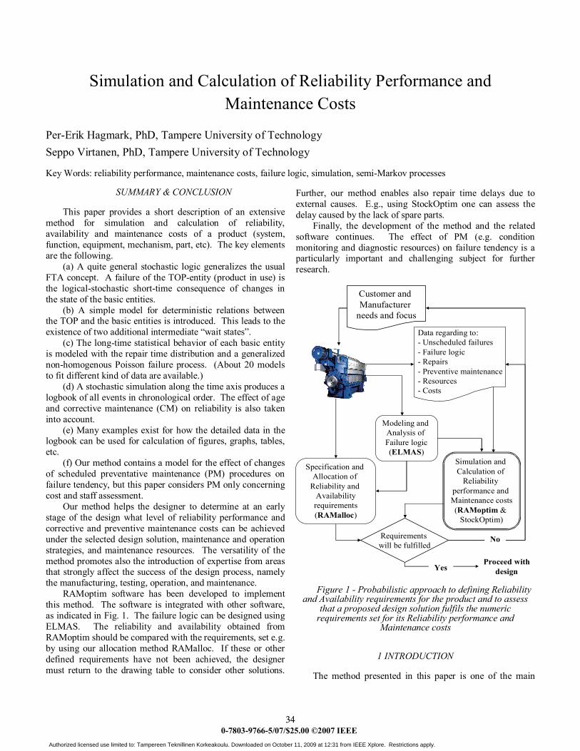
This paper provides a short description of an extensive method for simulation and calculation of reliability, availability and maintenance costs of a product (system, function, equipment, mechanism, part, etc). The key elements are the following.
(a) A quite general stochastic logic generalizes the usual FTA concept. A failure of the TOP-entity (product in use) is the logical-stochastic short-time consequence of changes in the state of the basic entities.
(b) A simple model for deterministic relations between the TOP and the basic entities is introduced. This leads to the existence of two additional intermediate “wait states”.
(c) The long-time statistical behavior of each basic entity is modeled with the repair time distribution and a generalized non-homogenous Poisson failure process. (About 20 models to fit different kind of data are available.)
(d) A stochastic simulation along the time axis produces a logbook of all events in chronological order. The effect of age and corrective maintenance (CM) on reliability is also taken into account.
(e) Many examples exist for how the detailed data in the logbook can be used for calculation of figures, graphs, tables, etc.
(f) Our method contains a model for the effect of changes of scheduled preventative maintenance (PM) procedures on failure tendency, but this paper considers PM only concerning cost and staff assessment.
Our method helps the designer to determine at an early stage of the design what level of reliability performance and corrective and preventive maintenance costs can be achieved under the selected design solution, maintenance and operation strategies, and maintenance resources. The versatility of the method promotes also the introduction of expertise from areas that strongly affect the success of the design process, namely the manufacturing, testing, operation, and maintenance.
RAMoptim software has been developed to implement this method. The software is integrated with other software, as indicated in Fig. 1. The failure logic can be designed using ELMAS. The reliability and availability obtained from RAMoptim should be compared with the requirements, set e.g. by using our allocation method RAMalloc. If these or other defined requirements have not been achieved, the designer must return to the drawing table to consider other solutions.
Further, our method enables also repair time delays due to external causes. E.g., using StockOptim one can assess the delay caused by the lack of spare parts.
Finally, the development of the method and the related software continues. The effect of PM (e.g. condition monitoring and diagnostic resources) on failure tendency is a particularly important and challenging subject for further research.
Figure 1 - Probabilistic approach to defining Reliability
and Availability requirements for the product and to assess that a proposed design solution fulfils the numeric
requirements set for its Reliability performance and Maintenance costs
1 INTRODUCTION
The method presented in this paper is one of the main
Customer and Manufacturer
needs and focus
Requirements will be fulfilled
No
Yes
Data regarding to:- Unscheduled failures- Failure logic- Repairs- Preventive maintenance- Resources- Costs
Modeling and Analysis of Failure logic(ELMAS)
Simulation and Calculation of
Reliability performance and Maintenance costs(RAMoptim &
StockOptim)
Specification and Allocation of
Reliability and Availabilityrequirements (RAMalloc)
Proceed with design
0-7803-9766-5/07/$25.00 ©2007 IEEE 34
Authorized licensed use limited to: Tampereen Teknillinen Korkeakoulu. Downloaded on October 11, 2009 at 12:31 from IEEE Xplore. Restrictions apply.

Journal of Power Sources 171 (2007) 46–54
Reliability analysis and initial requirements for FC systems and stacks
K. Astrom a,∗, E. Fontell a, S. Virtanen b
a Wartsila Corporation, Tekniikantie 14, FIN-02150 Espoo, Finlandb Tampere University of Technology, Korkeakoulunkatu 6, FIN-33101 Tampere, Finland
Received 12 September 2006; accepted 21 November 2006Available online 5 January 2007
Abstract
In the year 2000 Wartsila Corporation started an R&D program to develop SOFC systems for CHP applications. The program aims to bringto the market highly efficient, clean and cost competitive fuel cell systems with rated power output in the range of 50–250 kW for distributedgeneration and marine applications.
In the program Wartsila focuses on system integration and development. System reliability and availability are key issues determining thecompetitiveness of the SOFC technology. In Wartsila, methods have been implemented for analysing the system in respect to reliability and safetyas well as for defining reliability requirements for system components. A fault tree representation is used as the basis for reliability predictionanalysis. A dynamic simulation technique has been developed to allow for non-static properties in the fault tree logic modelling.
Special emphasis has been placed on reliability analysis of the fuel cell stacks in the system. A method for assessing reliability and critical failurepredictability requirements for fuel cell stacks in a system consisting of several stacks has been developed. The method is based on a qualitativemodel of the stack configuration where each stack can be in a functional, partially failed or critically failed state, each of the states having differentfailure rates and effects on the system behaviour. The main purpose of the method is to understand the effect of stack reliability, critical failurepredictability and operating strategy on the system reliability and availability. An example configuration, consisting of 5 × 5 stacks (series of 5sets of 5 parallel stacks) is analysed in respect to stack reliability requirements as a function of predictability of critical failures and Weibull shapefactor of failure rate distributions.© 2006 Elsevier B.V. All rights reserved.
Keywords: Reliability analysis; Fault tree analysis; SOFC system; Stack reliability
1. Introduction
Increasing customer awareness of reliability and its influenceon lifetime costs and safety, together with increasing complexityof industrial plants and equipment has resulted in an escalat-ing need for systematic methods of accounting for reliability indesign and manufacturing. Traditionally, the use of such meth-ods has essentially been limited to aviation, space and nuclearapplications. More recently these methods have been adaptedin several other industry branches. Reliability is expected to
Abbreviations: ac, alternating current; BoP, balance of plant; CHP, combinedheat and power; dc, direct current; FMEA, failure mode and effect analysis; FTA,fault tree analysis; HAZOP, Hazard and Operability Analysis; MTBF, mean timebetween failure; MTTF, mean time to fail; R&D, research and development;SOFC, solid oxide fuel cell; VBA, Visual Basic for Applications; WFC, Wartsilafuel cell
∗ Corresponding author. Tel.: +358 10 709 5473; fax: +358 10 709 5440.E-mail address: [email protected] (K. Astrom).
become a key competitive factor in applications where safetyand availability are important [1].
Since the year 2000, Wartsila has developed planar SOFCsystems for distributed power generation and marine applica-tions. Wartsila focuses on system design and integration, balanceof plant (BoP) development, and the interface between the SOFCpower unit and the application. The SOFC stack being an inte-grated part of the FC system, optimal interaction between thestack and the BoP is an essential part of system optimization,which calls for close cooperation between the stack manufac-turers and system integrators. Wartsila Corporation and HaldorTopsøe A/S, whose fuel cell program is managed by Topsøe FuelCell A/S, are running a joint development program within theplanar SOFC technology. The program aims to bring highly effi-cient, clean, reliable and cost-competitive fuel cell products tothe market for stationary power generation and marine applica-tions. Within the program, a conceptual study of a 250 kW planarSOFC system for combined heat and power (CHP) applicationswas presented in 2003 [2], along with strategies to counter-
0378-7753/$ – see front matter © 2006 Elsevier B.V. All rights reserved.doi:10.1016/j.jpowsour.2006.11.085

708
Spare part stock asset management by stochastic simulation
P.-E. Hagmark Tampere University of Technology
Korkeakoulunkatu 6 Box 589, FIN-33101 Tampere, Finland
[email protected] H. Pernu
Tampere University of Technology Korkeakoulunkatu 6
Box 589, FIN-33101 Tampere, Finland [email protected]
ABSTRACT: The design of a spare part inventory is a multi-phase task including contradic-tory economical and technical requirements. New methods and software for this area of prob-lems have been developed in Tampere University of Technology in collaboration with Finnish industry. The inventory model to be presented is an effort toward a concrete and broad-based methodology. A practical example as well as comparisons with the current literature is also given.
The model can be characterized as a versatile simulation-calculation scheme that connects spare part consumption, storage costs, and shortage probability and costs with existing maintenance strategies e.g. corrective, preventive and predictive maintenance. Stochastic simulation in the sub-models imitates the reality in time order, and the multitude of variables and concepts makes the model flexible for interpretations and new features. The inventory policy is ‘continuous review’, and the actors are: one stock, one critical part (or group of parts), one or more part suppliers, and one or more part consumers (customers).
The software developing around the model increases continuously the applicability. At present, automatic optimization of any selected cost combination can be performed, and the set of partaking variables will gradually be extended. Constraint checking during optimization has also been implemented to some extent.
KEYWORDS: Inventory design and control, stock asset management, spare parts, stochastic simulation, genetic algorithm.
1. INTRODUCTION
Spare part inventory control and management has been intensively researched for many decades. Extensive literature and research reports have been published. Kennedy et al. (2002) have pro-vided a comprehensive literature overview. A large part of the reported methods seem to be case specific and restrictive in scope. The model in question consists often of a few analytic-numeric formulas and a small number of variables.
Simulation-based and more versatile models exist, but a more comprising methodology would be desirable. Our model contributes to a generic approach. The kernel, a time-ordered simulation-calculation scheme (Fig. 1), is readily open for extensions and new details, and not so exposed to distorting and restricting assumptions as analytic-numeric methods. The inventory policy is based on continuous review. The actors are one stock, one critical part (or group of parts), one or more part suppliers, and one or more part consumers (customers).
We start with a superficial description following Figure 1 below. The first module, PartRel, offers several methods for the construction of life distributions for different stress levels.
©The 2nd World Congress on Engineering Asset Management (EAM) and The 4th International Conference on Condition Monitoring
Available online at www.sciencedirect.com
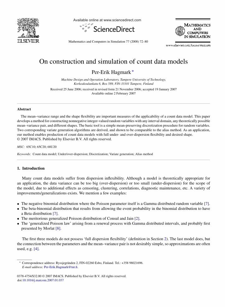
Mathematics and Computers in Simulation 77 (2008) 72–80
On construction and simulation of count data models
Per-Erik Hagmark ∗Machine Design and Operation Laboratory, Tampere University of Technology,
Korkeakoulunkatu 6, Box 589, FIN-33101 Tampere, Finland
Received 25 June 2006; received in revised form 21 November 2006; accepted 19 January 2007Available online 2 February 2007
Abstract
The mean–variance range and the shape flexibility are important measures of the applicability of a count data model. This paperdevelops a method for constructing nonnegative integer-valued random variables with any interval domain, any theoretically possiblemean–variance pair, and different shapes. The basic tool is a simple mean-preserving discretization procedure for random variables.Two corresponding variate generation algorithms are derived, and shown to be comparable to the alias method. As an application,our method enables production of count data models with full under- and over-dispersion flexibility and desired shape.© 2007 IMACS. Published by Elsevier B.V. All rights reserved.
MSC: 65C10; 65C20; 68U20
Keywords: Count data model; Under/over-dispersion; Discretization; Variate generation; Alias method
1. Introduction
Many count data models suffer from dispersion inflexibility. Although a model is theoretically appropriate foran application, the data variance can be too big (over-dispersion) or too small (under-dispersion) for the scope ofthe model, due to additional effects as censoring, clustering, correlations, diagnostic maintenance, etc. A variety ofimprovements/generalizations exists. We mention a few examples:
• The negative binomial distribution where the Poisson parameter itself is a Gamma distributed random variable [7].• The beta-binomial distribution that results from allowing the event probability in the binomial distribution to have
a Beta distribution [7].• The meritorious generalized Poisson distribution of Consul and Jain [2].• The ‘generalized Poisson law’ arising from a renewal process with Gamma distributed intervals, and probably first
presented by Morlat [8].
The first three models do not possess ‘full dispersion flexibility’ (definition in Section 2). The last model does, butthe connection between the parameters and the mean–variance pair is not desirably simple, so approximations are oftenused, e.g. [4].
∗ Correspondence address: Ryssjegranden 2, FIN-02260 Esbo, Finland. Tel.: +358 98021696.E-mail address: [email protected].
0378-4754/$32.00 © 2007 IMACS. Published by Elsevier B.V. All rights reserved.doi:10.1016/j.matcom.2007.01.037
DETERMINING RELIABILITY PERFORMANCE AND MAINTENANCE COSTS OF SELECTED DESIGN SOLUTION AND MAINTENANCE STRATEGY
Seppo Virtanena and Per-Erik Hagmarkb
a, bTampere University of Technology, Korkeakoulunkatu 6, FI-33101 Tampere, Finland
This paper discusses the application of a developed method for determining the reliability performance and maintenance costs of selected design solution and maintenance strategy. Along with the conceptual presentation we follow numerical results of a power generation unit (PGU) which is our case example. With the help of the method, the engineer can determine the early stage of the development project to which level of reliability performance and maintenance costs can be achieved by using the selected design solution and maintenance strategy. If the defined requirements have not been achieved, the engineer must go back to the drawing table to consider other solutions and/or maintenance strategy for achieving the requirements. The method is one of the main results from the research project, which has been carried out in collaboration with eleven top Finnish industrial companies. The applicability of the method has been tested in the companies participating in the research project. Ramentor (www.ramentor.com) is responsible for commercializing, marketing and supplying technical support of the ELMAS software which has been developed to implement the method.
Key Words: Design Solution, Reliability Performance, Maintenance Strategy and Costs, Simulation, Calculation
1 INTRODUCTION
The outline of the paper is as follows. In section 2 we introduce our case example (PGU) and a developed method to model its failure logic. Three operation strategies concerning deterministic relationships between the TOP entity (PGU failure) and the basic entities, and a rescue mechanism for gates are introduced.
In section 3 we discuss the design for long-time statistical behaviour of the basic entities, i.e., repair time distributions and the point process for failures. Then, the parameters for the effect of age and corrective maintenance (CM) on the occurrence of failures are introduced. Thereafter the simulation process, consisting of simultaneous and interacting “semi-Markov-like” processes (one for each entity), can be started.
The simulation produces a detailed time-ordered logbook of all events, the raw material for subsequent calculation. Section 4 describes reliability and availability calculations for the PGU and its basic entities, and their relations. Many examples are given of how the detailed data in the logbook can be used for calculation of figures, graphs, and tables. After additional inputs and the definition concerning failures and preventive maintenance, section 5 discusses results on costs and resource calculation for both corrective and preventive maintenance. Finally the assessment of the variation of PGU’s part’s failure probability impact on its maintenance costs and reliability performance is introduced.
2 Failure and operation structures
2.1 Definition of PGU’s Failure Logic
The PGU which is our case example consists of two identical generators (GE1 and GE2) and a back-up generator (BUGE). GE1 and GE2 have to run simultaneously in order PGU to produce required output. In case GE1 or GE2 fails or either of them is taken to the maintenance service, BUGE is called for operation until GE1 or GE2 is repaired or the service is completed. BUGE can fail either in the star-up or running phases. GE1 or GE2 can be repaired or serviced concurrently while the other is still running. In case BUGE fails, the one running is not shut down.
A SIMULATION MODEL FOR OPTIMIZATION OF MAINTENANCE STRATEGY IN ASSET MANAGEMENT
Pernu H a and Hagmark P-E b
a Tampere University of Technology, Korkeakoulunkatu 6, 33101 Tampere, Finland.
b Tampere University of Technology, Korkeakoulunkatu 6, 33101 Tampere, Finland.
The optimization of the maintenance strategy of a company is a multi-phase task including contradictory economical and technical requirements. A new simulation model for this area of problems has been developed in Tampere University of Technology in collaboration with Finnish industry. The simulation model can be used for determining the reliability requirements of the system under study (manufacturer’s viewpoint), for determining the maintenance strategy of the system (owner’s viewpoint), and for balancing warranty and the risk of failure (manufacturer’s and service provider’s viewpoint).
The primary concepts of the model are scheduled preventive maintenance (PM), unexpected preventive maintenance (UPM), corrective maintenance (CM) (when a breakdown has occurred), and system’s usage and cost profiles during the calendar year. The model connects these concepts by using a multitude of variables, which make the model flexible for interpretations. Stochastic simulation imitates the reality through the life cycle of the system.
A critical rolling bearing of a ship propulsion system is used for demonstration. The stochastic failure propagation mechanism after failure detection gives room for a dynamic docking scheduling scheme for cost minimization. The maintenance model is based on replacement of the bearing at regular PM docking and possibly extra replacements at UPM dockings. The failure model is divided into two parts; service life i.e. the lifetime before the detection of a failure and remaining life i.e. the time before the final breakdown of the bearing. If the service life of the bearing ends before the next scheduled PM, and if the remaining life ends with a breakdown, then the ship is unavailable until the planned UPM.
In the model the cost of a replacement is fixed, and operator’s shortage costs depend on the season when the maintenance takes place. By varying the maintenance strategies, the total cost minimization can be performed. In addition to the cost minimization and the maintenance strategy specification, the simulation model is a tool for evaluation of the risk of unexpected failure against the selected warranty terms.
Key Words: Life model, Maintenance, Optimization, Reliability, Simulation, Unavailability cost, Warranty
1 INTRODUCTION
Modeling and analysis of failures form a foundation for quantitative investigation of the reliability, availability and costs of a design entity, e.g. a system, equipment, mechanism, part, or part location. The method presented in this paper can be applied to many kinds of entities, whose failing can be modeled by two consecutive independent stochastic events: The first event is related to the end of normal operation when the failure is observed, and the second event to the growth of failure until the final breakdown. The entity to be studied in this paper is a thrust bearing of the propulsion system of a cruise ship.

PRODUCT RELIABILITY AND AVAILABILITY IN FIELD DATA
Nevavuori L
Service Development, KONE Corporation, Myllykatu 3, Hyvinkää 05801, Finland
KONE is one of the world’s leading elevator and escalator companies. It provides customers with industry-leading elevators and escalators and innovative solutions for maintenance and modernization. KONE was established 1910 in Finland. Currently the company has approximately 32,500 employees.
Demands for the dependability have risen in the elevator industry during the recent years. The aim of the paper is to introduce a case study that was performed by KONE’s reliability and maintenance departments in the beginning of year 2007. The case is about products’ perceived dependability follow-up. Moreover, a target is to present how reliability data was collected as well as utilized in reliability centered maintenance planning. In this case the starting point for a dependability follow-up was the back reported field data from maintenance actions.
One of the main objectives of the case was to construct a new method for modeling the lifetime of a component based on the failure data. In the first phase of the case study, a reliability function was modeled for the studied component by utilizing the Kaplan-Meier estimation method. Both complete and censored lifetime observations were exploited. In the second phase, the cost factors of corrective and preventive maintenance were evaluated. Then, by utilizing the modeled reliability function and simulation software the most suitable maintenance strategy for the component was optimized.
The paper summarizes the experiences collected from the methods of the case study. As the second conclusion, requirements and advantages for a systematic dependability follow-up process are outlined. It is generally clarified which are the main challenges to utilize field data, and how back reporting procedures and follow-up tools can be developed in the industry.
Key Words: Field data, Reliability engineering, RCM
1 INTRODUCTION
Customers expect reliable products. The reputation of a company can be lost in a short time, if a product fails dramatically. KONE has researched reliability many years as a part of product development and adopted several methods to increase the degree of durability of products. However, the designed reliability of elevators is not the only factor relating to finally perceived dependability. Also manufacturing, transportation, installation, and maintenance as well as operational environment have effects on dependability [1]. To understand previous effects a large number of different field data studies were performed for MonoSpace elevators, the one of KONE’s global volume products. The first release of MonoSpace was introduced in 1996. It was the world's first affordable and efficient “machine-room-less” elevator concept. It is operated by a disc-shaped KONE EcoDisc™ hoisting machine which fits inside a standard elevator hoist way.
The performed field data analyses have identified that elevator cabin lighting failure is one of the most frequently reported call-out root cause in MonoSpace elevators. A term call-out is defined by: “Any request for an intervention coming from a customer or a remote monitoring system, which triggers a repair visit to equipment by a service technician”. KONE aims to
Investment in new product reliability
D.N.P. Murthy a,�, M. Rausand b, S. Virtanen c
a Division of Mechanical Engineering, The University of Queensland, Brisbane, Australiab Department of Production and Quality, Norwegian University of Science and Technology, Trondheim, Norwayc Institute of Machine Design and Operation, Tampere University of Technology, Tampere, Finland
a r t i c l e i n f o
Article history:
Received 28 April 2007
Received in revised form
25 January 2009
Accepted 28 February 2009Available online 26 March 2009
Keywords:
Product reliability
Product development
Reliability design
Product life cycle
Mathematical models
a b s t r a c t
Product reliability is of great importance to both manufacturers and customers. Building reliability into
a new product is costly, but the consequences of inadequate product reliability can be costlier. This
implies that manufacturers need to decide on the optimal investment in new product reliability by
achieving a suitable trade-off between the two costs. This paper develops a framework and proposes an
approach to help manufacturers decide on the investment in new product reliability.
& 2009 Elsevier Ltd. All rights reserved.
1. Introduction
Modern industrial societies are characterised by new productsappearing on the market at an ever increasing pace. Some of thereasons for this are (i) rapid advances in technology, (ii) increasingconsumer expectations and, (iii) global competition. As a result,the complexity of products and the cost of product developmentare increasing and the product life cycle is getting shorter witheach new generation. Consumers are getting more concerned withthe performance of the product over its useful life, and increasingpower of consumer groups has resulted in stronger legislation toprotect consumer interests. All of these have implications formanufacturers of all kinds (consumer, commercial and industrial)of products.
A product is designated by its characteristics and attributes.The distinction between these two is best explained by thestatement ‘‘product characteristics physically define the productand influence the formation of product attributes; productattributes define consumer perceptions and are more abstractthan characteristics’’ from Tarasewich and Nair [1]. Consumersview products in terms of attributes.
The reliability of a product is a characteristic, which conveysthe notion of dependence or absence of failure. Unreliability is theopposite. According to IEC 60050-191 [2], the reliability of aproduct (system) is the probability that the product (system) will
perform its intended function for a specified time period whenoperating under normal (or stated) environmental conditions.
One way for manufacturers to assure consumers about productperformance is through warranty. A warranty is a contractualobligation, which requires the manufacturer to rectify, replaceor provide compensation, should the product not performsatisfactorily over the warranty period. It can be viewed as aproduct characteristic that serves two important roles for amanufacturer—(i) to signal product reliability (as better warrantyterms indicate a more reliable product) and, (ii) to differentiatethe product from competitors as warranty is bundled with theproduct and sold as a an element of product support.
Product reliability depends on the decisions made during thedesign and production of the product. Building-in productreliability is costly as it involves considerable expenditure duringthe design, development and production phases of the productlife cycle. Not having adequate reliability is costlier as failuresresult not only in higher warranty costs but also reduced salesand revenue due to the negative impact of customer dissatisfac-tion resulting from product failures. As reported in WarrantyWeek [3] the warranty costs vary from 1% to 4% of sale pricedepending on the product and the manufacturer. Viewed as afraction of profits, this figure jumps by an order of magnitude.In the long run it affects the reputation of the manufacturer,impacts on the bottom line of the balance sheet and the survivalof the manufacturer. From the customer’s point of view,unreliability reduces availability and increases maintenance costsover the useful life of the product. This implies that manufacturersneed to decide on the investment in product reliability from anoverall business viewpoint. This topic has received some limited
ARTICLE IN PRESS
Contents lists available at ScienceDirect
journal homepage: www.elsevier.com/locate/ress
Reliability Engineering and System Safety
0951-8320/$ - see front matter & 2009 Elsevier Ltd. All rights reserved.
doi:10.1016/j.ress.2009.02.031
� Corresponding author.
E-mail address: [email protected] (D.N.P. Murthy).
Reliability Engineering and System Safety 94 (2009) 1593–1600

Product variety and reliability
D.N.P. Murthy a,�, P.-E. Hagmark b, S. Virtanen b
a Division of Mechanical Engineering, The University of Queensland, Brisbane, Australiab Institute of Machine Design and Operation, Tampere University of Technology, Tampere, Finland
a r t i c l e i n f o
Article history:
Received 28 April 2007
Received in revised form
25 January 2009
Accepted 28 February 2009Available online 26 March 2009
Keywords:
Product reliability
Business objectives
Customer satisfaction
Sales
Warranty
a b s t r a c t
Murthy et al. [Murthy DNP, Rausand M, Virtanen S. Investment in new product reliability, Reliability
Engineering & System Safety (accepted for publication)] proposed an approach to decide on product
reliability in the context of new product development and identified two tasks for execution as part of
the overall process. In this paper, we focus on the first task—determining the product reliability
requirements.
& 2009 Elsevier Ltd. All rights reserved.
1. Introduction
Building product reliability is costly but not having adequatereliability can be costlier. Murthy et al. [1] developed a framework(which integrates various technical and commercial elements)and proposed an approach (involving product life cycle perspec-tive and use of mathematical models) to decide on the optimalinvestment in new product reliability. This involves decisionmaking during the execution of the following two tasks.
� Task 1: Defining the reliability requirements at the productlevel.� Task 2: Deriving the reliability specifications at the component
level.
Product reliability depends on the usage rate, operatingenvironment and many other variables. When these vary signi-ficantly, a strategy for the manufacturer is to build a variety ofproducts (with differing reliabilities) instead of a single product.
In this paper, we focus on Task 1 and look at product variety,and the reliability for each type, using the framework andapproach discussed in [1]. The outline of the paper is as follows.We start with a brief discussion of product variety in Section 2.Section 3 looks at product reliability and the modelling of it.Deciding on the product reliability involves solving an optimisa-tion problem with reliability and non-reliability decision variables
and is discussed in Section 4. We illustrate by looking at two casesin Sections 5 and 6. In Section 7 we discuss the softwaredeveloped for executing Task 1 as part of the BRED project atthe Tampere University of Technology. Section 8 deals with someconcluding comments.
2. Product variety
When needs vary significantly across the customer population,achieving the business objectives with a single product designmight not be possible. In this case, the optimal strategy is to offera variety of products using a common product platform. Productvariety is achieved by variations in the attributes and/orcharacteristics. For example, in the case of washing machine, itcould be the load (kilogram per wash) leading to small, mediumand large machines and in the case of photocopier it could be thethroughput (number of pages printed per minute) leading to slowand high-speed printers. There is a vast literature on productvariety and these deal with many different issues, see for example,[2–9]. In this paper we focus on variety where products differ intheir reliability characteristics.
3. Product reliability
Let F(t;y) denote the distribution function for the time to firstfailure. The reliability of the product is given by R(t;y) ¼ 1�F(t;y).Let f(t;y) and h(t;y) denote the density and hazard functionsassociated with F(t;y).
ARTICLE IN PRESS
Contents lists available at ScienceDirect
journal homepage: www.elsevier.com/locate/ress
Reliability Engineering and System Safety
0951-8320/$ - see front matter & 2009 Elsevier Ltd. All rights reserved.
doi:10.1016/j.ress.2009.02.030
� Corresponding author.
E-mail address: [email protected] (D.N.P. Murthy).
Reliability Engineering and System Safety 94 (2009) 1601–1608

Component reliability specification
D.N.P. Murthy a,�, T. Østeras b, M. Rausand b
a Division of Mechanical Engineering, The University of Queensland, Brisbane Q 4072, Australiab Department of Production and Quality, Norwegian University of Science and Technology, Trondheim, Norway
a r t i c l e i n f o
Article history:
Received 28 April 2007
Received in revised form
25 January 2009
Accepted 28 February 2009Available online 26 March 2009
Keywords:
Reliability specification
Redundancy
Preventive maintenance
Development
a b s t r a c t
Building reliability into a product is costly and needs to be traded against the consequences of product
unreliability. This article is the third in a series of three articles, where the first deals with optimal
investment in reliability, which involves executing two tasks—(i) deciding on the reliability
requirements and (ii) deciding on component specifications (SP) to achieve the desired reliability.
The second article deals with the first task and in this third article, we focus on the second task.
& 2009 Elsevier Ltd. All rights reserved.
1. Introduction
Product reliability is of importance to both manufacturers andconsumers since inadequate reliability results in higher costs toboth parties. Murthy et al. [1] examine this issue and look at theoptimal investment in reliability. It involves two tasks—(i)deciding on the reliability requirements and (ii) deciding oncomponent specifications (SP) to achieve the desired reliability.Murthy et al. [2] deal with the first task and in this article wediscuss the second task.
The design process defines how the product is to be built. Thisinvolves decomposing the product, starting at the product leveland proceeding down to the component level, with severalintermediate levels. At each level there are several elements.The specification of an element at any level is derived from theperformance of the elements at the level above it. As a result,there is a sequence of performances and specifications that leadsto specifications at the component level.
In this article we focus on the sequence of performances andspecification throughout the design process, and define thereliability specification at the component level that will ensurethat the product reliability requirements are met. The outline ofthe article is as follows. We start with a brief general discussion ofperformance and specification and the links between the two inthe context of new product development in Section 2. This isfollowed by a brief discussion of the design process in Section 3.Section 4 deals with the process of arriving at the reliabilityspecifications at the component level. Two key elements of theprocess are discussed in the next two sections. In Section 5, we
look at reliability allocation and the alternative options to ensurethat the target values assigned for component reliability areachieved. Section 6 deals with optimal decision making inreliability specification at component level.
2. Performances and specifications
2.1. Definitions
There are several different notions of performance andspecifications in the context of the new product developmentprocess and these are discussed in detail in [3]. We confine ourattention to a subset of these that is relevant for deriving thereliability specification at component level:
� Desired performance (DP) is a statement about the performancedesired from an object (product or component).� Specifications describe how the desired performance can be
achieved (using a synthesis process involving evaluation ofpotential solutions to select the best), with desired perfor-mance as input to the process.� Predicted performance (PP) is an estimate of the performance of
the object for a given set of specifications.
2.2. Relationship between performance and specifications
Performance and specifications are strongly interlinked,and play a central role in the new product development process(e.g., [4–6] discuss the critical importance of performance and
ARTICLE IN PRESS
Contents lists available at ScienceDirect
journal homepage: www.elsevier.com/locate/ress
Reliability Engineering and System Safety
0951-8320/$ - see front matter & 2009 Elsevier Ltd. All rights reserved.
doi:10.1016/j.ress.2009.02.029
� Corresponding author.
E-mail address: [email protected] (D.N.P. Murthy).
Reliability Engineering and System Safety 94 (2009) 1609–1617
Statistics and Probability Letters 79 (2009) 1120–1124
Contents lists available at ScienceDirect
Statistics and Probability Letters
journal homepage: www.elsevier.com/locate/stapro
A new concept for count distributionsPer-Erik Hagmark ∗Machine Design and Operation Laboratory, Tampere University of Technology, Korkeakoulunkatu 6, Box 589, FIN-33101 Tampere, Finland
a r t i c l e i n f o
Article history:Received 5 December 2008Received in revised form 5 January 2009Accepted 5 January 2009Available online 20 January 2009
MSC:60E0560-0815A0970C20
a b s t r a c t
A new concept, called silhouette, and the related parameterization are introduced andstudied. Applications show how to extend maximally the mean–variance domain of acount distribution, and how to construct a single variable for any mean–variance and anyrequirements on distribution shape.
© 2009 Elsevier B.V. All rights reserved.
1. Introduction
We consider count variables, i.e. nonnegative integer-valued random variables, whose meanµ and deviation σ are finite.A µσ -domain, i.e. the set of all pairs (µ, σ ) of a set of count variables, will be called maximal if it contains all pairs (µ, σ )satisfying
(µ− [µ]) ([µ] + 1− µ) < σ 2 < µ (N − µ) , (1)
where N is the supremum of the variables (possibly N = ∞, and [µ] is the largest integer not exceeding µ. On the otherhand, no µσ -domain exceeds the closure of (1).In commonly used count distributions, the µσ -domain is very seldom maximal, and good general shape flexibility is
practically non-existent. In count data modeling this can mean that the µσ -domain of the planned model does not containthe mean–deviation pair estimated from the data, or that no distribution shape offered by the model matches the data.The famous distribution of Consul and Jain (1973) is a typical example with seriously incomplete underdispersion ability,i.e. σ stays on a nonzero distance from the left side of (1). The so-called ‘generalized Poisson law’ again does have maximalµσ -domain, but the shape is always unimodal, and besides, the relations between the parameters and the µσ -pair arelaborious (Morlat, 1952; Winkelmann, 1995). For theory and practice of count models, see e.g. Johnson et al. (1992), Ridoutand Besbeas (2004), Castillo and Perez-Casany (2005), and Hagmark (2008).This study develops a new general approach. We introduce a new concept, the ‘silhouette’, and a related one-parameter
extension for non-binary bounded count variables. Basic theoretical results with examples are presented in Sections 2–5,applications follow in Sections 6–8, and a summary in Section 9.
2. Basic concepts and formulas
Let F0, F1, F2, . . . be a non-decreasing sequencewith 0≤ Fn ≤ 1 and limn→∞ Fn = 1. In otherwords, Fn is the (cumulative)distribution of a count variable (Cv). The related sequence Y0 = 0, Yn+1 = Yn + Fn will be called integral distribution (Id).
∗ Corresponding address: Ryssjegränden 2, FIN-02260 Esbo, Finland. Tel.: +358 0 98021696.E-mail address: [email protected].
0167-7152/$ – see front matter© 2009 Elsevier B.V. All rights reserved.doi:10.1016/j.spl.2009.01.006
KOTEL 256
Total number of pages in Appendix 11
APPENDIX 2
MASTER THESIS
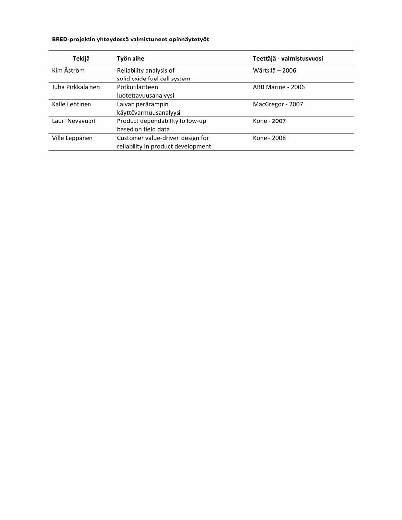
BRED‐projektin yhteydessä valmistuneet opinnäytetyöt
Tekijä Työn aihe Teettäjä ‐ valmistusvuosi
Kim Åström Reliability analysis of solid oxide fuel cell system
Wärtsilä – 2006
Juha Pirkkalainen Potkurilaitteen luotettavuusanalyysi
ABB Marine ‐ 2006
Kalle Lehtinen Laivan perärampin käyttövarmuusanalyysi
MacGregor ‐ 2007
Lauri Nevavuori Product dependability follow‐up based on field data
Kone ‐ 2007
Ville Leppänen Customer value‐driven design for reliability in product development
Kone ‐ 2008

Kim Åström
Reliability Analysis of Solid Oxide Fuel Cell System
Master's thesis submitted in partial fulfilment of the requirements for the degree of Master of
Science in Technology
Espoo, 13.02.2006
Supervisor: Prof. Peter Lund
Instructor: Prof. Seppo Virtanen

ii
HELSINKI UNIVERSITY OF TECHNOLOGY ABSTRACT OF MASTER’S THESIS Department of Engineering Physics and Mathematics PO Box 2200, FIN-02150 HUT, FINLAND 13.02.2006
Author: Kim Åström
Department: Major Subject: Minor Subject:
Engineering Physics and Mathematics Advanced Energy Systems Power Electronics
English title:
Finnish title: Number of Pages:
Reliability Analysis of Solid Oxide Fuel Cell System
Kiinteäoksidipolttokennojärjestelmän luotettavuusanalyysi
65
Chair: Supervisor: Instructor:
Tfy-56 Advanced Energy Systems Prof. Peter Lund Prof. Seppo Virtanen
Abstract: Fuel cells are energy conversion devices with potential for high efficiencies with low emissions. Solid oxide fuel cells (SOFC) are seen as one of the most promising technologies for distributed combined heat and power production (CHP).
Wärtsilä is developing a 20kW SOFC prototype unit aimed for demonstration in various application environments by 2007-2008. Accounting for reliability related issues has been adapted as an important aspect of the system design. Increasing customer awareness of these issues has highlighted the need for systematic methods for accounting for reliability in design and manufacturing. In the SOFC system, the importance of reliability is further pronounced by safety and durability considerations.
In this thesis, different methodologies deployed in reliability engineering are discussed, with special emphasis on their applicability for analysing the SOFC system. A combination of different methodologies is chosen and implemented. A fault tree approach is chosen for describing the logical interrelations between failures and consequences. An extensive failure mode and effects analysis (FMEA) formed the foundation for constructing the fault tree. A simulation tool has been implemented for dynamic modelling of the system in respect to failures and hazards. A customized model for analysing the fuel cell stacks is implemented.
This thesis provides the theoretical foundation based on which the developed methods have been successfully applied for analysis of the SOFC system.
Keywords: Reliability analysis, simulation, solid oxide fuel cell
Study secretary fills:
Thesis approved: Library code:
TAMPEREEN TEKNILLINEN YLIOPISTO
Konetekniikan osasto
JUHA PIRKKALAINEN
POTKURILAITTEEN LUOTETTAVUUSANALYYSI
Diplomityö
Tarkastaja prof. Seppo Virtanen
Määrätty osastoneuvoston kokouksessa
16.8.2006

TIIVISTELMÄ
TAMPEREEN TEKNILLINEN YLIOPISTO Konetekniikan osasto / Koneensuunnittelu PIRKKALAINEN, JUHA: Potkurilaitteen luotettavuusanalyysi Diplomityö, 66s., 23 liites. Tarkastaja: prof. Seppo Virtanen Rahoittaja: ABB Marine Oy Syyskuu 2006
Hakusanat: luotettavuus, toimintavarmuus, potkurilaite
Tässä työssä on toteutettu sähköisellä perämoottoriperiaatteella toimivan laivan potkuri-
laitteen Azipod Large-propulsiojärjestelmän luotettavuusanalyysi. Työn päätavoitteena
on ollut identifioida kohteesta kriittisimmät epäluotettavuuden riskitekijät, jotka voivat
johtaa laivan kuivatelakoimiseen viiden vuoden tarkasteluvälin aikana. Samalla on py-
ritty luomaan uusi toimintamalli erilaisten epäluotettavuuden riskitekijöiden määrittämi-
seen ja hallintaan ABB Marine:n tuotekehityksen sekä suunnittelun tarpeisiin.
Työ on jaettu kvalitatiivisiin ja kvantitatiivisiin tarkasteluihin. Kvalitatiivisissa vaiheissa
on laadittu kohteesta vikapuuanalyysit ELMAS-ohjelman avulla. Vikapuuanalyysien
avulla on tunnistettu kohteesta epäluotettavin osajärjestelmä ja siinä olevat kuivatela-
koimiseen johtavat kriittisimmät epäluotettavuuden riskitekijät. Kvantitatiivisessa osuu-
dessa on tutkittu epäluotettavimman osajärjestelmän ja sen kriittisten epäluotettavuuste-
kijöiden luotettavuusvaatimusten hallintaa RAMalloc-ohjelman avulla.
Ensisijaisesti työn tulokset osoittivat inhimillisten tekijöiden merkityksen kuivatelakoin-
tiriskin suuruuteen suhteessa tekniikkaan. Inhimillisistä riskitekijöistä merkittävimpiä
olivat erilaiset kokoonpanon ja valmistuksen aikana tapahtuvat inhimilliset virheet, joi-
den yhteydessä kriittisiin kohteisiin jää erilaisia epäpuhtauksia. Käyttö- ja huoltovirheet
osoittautuivat myös kriittisiksi. Tekniikan osalta merkittävimmät riskitekijät ovat irto-
osien aiheuttama oikosulkuvaara päämoottorilla ja magnetointikoneella sekä painelaa-
kerin voitelulinjan toimintavarmuus laakereiden eliniän takaamiseksi.
Työssä toteutetun toimintamallin avulla potkurilaitteen järjestelmäsuunnitteluun kuulu-
vien luotettavuusvaatimusten määrittäminen ja hallinta on mahdollista jatkossa toteuttaa
nykyistä perusteellisemmin.
KALLE LEHTINEN LAIVAN PERÄRAMPIN KAYTTÖVARMUUSANALYYSI Diplomityö Tarkastaja: Professori Seppo Virtanen Tarkastaja ja aihe hyväksytty Konetekniikan osastoneuvoston kokouksessa 14.2.2007

TAMPEREEN TEKNILLINEN YLIOPISTO Konetekniikan koulutusohjelma LEHTINEN, KALLE: Laivan perärampin käyttövarmuusanalyysi Diplomityö 57 sivua, 3 liitesivua Huhtikuu 2007 Pääaine: Kunnossapitotekniikka Tarkastaja: Professori Seppo Virtanen Avainsanat: Käyttövarmuus, laiva, peräramppi, luotettavuus, huollettavuus Laitteen käyttövarmuus muodostuu laitteelle suunnitellusta luotettavuudesta ja huollettavuudesta, sekä kunnossapito-organisaation huoltovarmuudesta. Käyttövarmuusanalyysissä tutkitaan näitä kaikkia kolmea käyttövarmuuden osatekijää. Tämän tutkimuksen tavoitteena on selvittää olemassa olevan laivan perärampin käyttövarmuutta kuvaavia tunnuslukuja ja keinoja käyttövarmuuden parantamiseksi. Käyttövarmuusanalyysin taustalla on halu selvittää huoltopalvelun tuottamisesta aiheutuvia kustannuksia ja löytää keinoja niiden pienentämiseksi. Laivan perärampin käyttövarmuusanalyysissä tutkittavalle kohteelle tehtiin vika- ja vaikutusanalyysi. Vika- ja vaikutusanalyysin tuloksia käytettiin lähtötietoina perärampin vikapuuanalyysin tekemisessä. Vikapuuta analysoitiin Tampereen teknillisessä yliopistossa kehitetyllä simulointimenetelmällä. Vikapuun simulointia varten kerättiin perärampin osilta vika ja korjaustietoa. Tämä tieto kerättiin pääasiassa asiantuntijahaastatteluin. Vikapuun simulointituloksista tunnistettiin perärampin käyttövarmuuden ja kunnossapitokustannusten kannalta kriittisimpiä osia. Kunnossapitokustannuksia katsottiin syntyvän ennakkohuollosta, korjaavasta kunnossapidosta ja epäkäytettävyydestä tulevista sopimussakoista. Käyttövarmuusanalyysin tuloksena saatiin myös laitteen hydraulijärjestelmään perustuva modulaarinen malli vikapuidenkin laatimista varten. Modulaarista mallia voidaan käyttää tehokkaasti hyväksi muiden laitteiden vikapuuanalyyseissä. Perärampin vikapuumallista kehitettiin myös malli perärampin vianhakua varten. Tätä rampin ohjausjärjestelmään perustuvaa mallia voidaan käyttää jatkossa kun kehitetään perärampin vianhakumenettelyjä. Perärampin käyttövarmuusanalyysin tulosten perusteella tehtiin päätelmiä perärampin käyttövarmuuden parantamiseen tähtäävistä tärkeimmistä toimenpiteistä. Tärkeimpinä toimenpiteinä nähtiin kunnossapitotiedon tarkempi kerääminen ja perärampin kunnossapitokustannusten kannalta kriittisimpien osien tarkempi vikaantumisen tutkiminen.

LAURI NEVAVUORI
PRODUCT DEPENDABILITY FOLLOW-UP BASED ON FIELD DATA
Master of Science Thesis
Examiner: Professor Seppo VirtanenExaminer and topic approved in the Mechanical Engineering Department Council meeting on 18 April 2007
II
ABSTRACT TAMPERE UNIVERSITY OF TECHNOLOGY Master’s Degree Programme in Mechanical Engineering NEVAVUORI, LAURI: Product Dependability Follow-up based on Field Data Master of Science Thesis, 84 pages, 2 Appendix pages August 2007 Major: Maintenance Engineering Examiner: Professor Seppo Virtanen Keywords: Reliability engineering, dependability, field data, maintenance Demands for the dependability have risen in the elevator industry during the recent years. This master‘s thesis examines products’ perceived dependability follow-up and reliability centred maintenance planning. A starting point for a follow-up is the back reported field data from maintenance actions, which includes for example the reason and target of the work as well as the performed actions. The aim of the thesis is to evaluate the current level of field data at Kone. Moreover, the possibility to utilise the data in maintenance planning is studied. One of the main objec-tives is to construct a method for modelling the lifetime of a component based on the failure data. The material for this study was collected from four countries, starting from year 2003. At the beginning, the extracted field data was analysed in general level. In addition, comparisons between countries were performed. The major part of the thesis consists of a dependability case study that was done for a component. The field data analyses showed that the component in question has caused a large number of failures that were detected by customers. In the first phase of the case study, a reliability function was modelled for the component. The Kaplan-Meier estima-tion method was utilised for modelling. After that, the cost factors of corrective and preventive maintenance were evaluated for the component. Then, by utilising the mod-elled reliability function and ELMAS and RAMoptim computer programs the most suit-able maintenance strategy for the component was optimised. The dependability simula-tions proved that preventive replacements of the component at the predefined intervals would improve dependability and decrease total maintenance costs. In the second phase of the case study a fault tree analysis was performed. The aim was to simulate the root causes of the component’s failures. The fault tree model was tested and it was found to be functional in failure analysis. A similar fault tree model could also be used in product design phase. It provides a possibility to compare the effects of different parts on the dependability of the designed product. In the conclusion of the thesis, there are outlined demands and advantages for more sys-tematic dependability follow-up process. The main demands include the further devel-opment of back reporting procedures and follow-up tools. In this way maintenance processes can be developed. Moreover, possibilities to improve product dependability would be achieved by increasing the number of preventive component replacements and the further development of remote monitoring utilisation. The experiences collected from the methods of the thesis and the reliability software used in preventive mainte-nance optimisation were promising.
VILLE LEPPÄNEN CUSTOMER VALUE-DRIVEN DESIGN FOR RELIABILITY IN PRODUCT DEVELOPMENT Master of Science Thesis
Examiners: Professor Olavi Uusitalo & Professor Seppo Virtanen Examiners and topic approved in the Faculty of Business and Technology Management Council meeting on 5 November 2008
II
ABSTRACT
TAMPERE UNIVERSITY OF TECHNOLOGY Master’s Degree Programme in Industrial Engineering and Management LEPPÄNEN, VILLE: Customer Value-Driven Design for Reliability in Product Development Master of Science Thesis, 87 pages, 9 Appendix pages April 2009 Major: Industrial Management Examiners: Professor Olavi Uusitalo & Professor Seppo Virtanen Keywords: Reliability, customer-perceived value, customer requirements, con-joint analysis, quality function deployment, product development
The elevator industry has become more aware of the importance of product reliability. In order to remain competitive in the market, companies need to direct their product de-velopment efforts into attributes providing the highest added value to customers. The purpose of this research was to assess the impact of elevator reliability on customer-perceived value, develop a methodology for translating customer perceptions into measurable reliability requirements of an elevator, and find effective means to imple-ment customer focus in the management of reliability requirements in product develop-ment at KONE.
The theoretical impact of reliability on customer-perceived value was studied by means of literature research. The methodology developed to translate customer perceptions into reliability requirements utilizes an adaptation of Conjoint Analysis, a self-developed method of rank-ordering failure effects and open-ended interview questions to capture customer views and preferences on reliability. Customer perceptions are then reflected on actual reliability performance of elevators by studying KONE maintenance records, and related to technical aspects for requirement specification utilizing an adap-tation of quality function deployment. The methodology also enables competitive analy-sis. Empirical evidence on the impact of elevator reliability on customer-perceived value was gathered by means of a case study using the developed methodology. The case study involved interviews of eight facility managers of high-rise buildings in the United Arab Emirates. Information on elevator reliability performance was researched by studying KONE maintenance records on high-rise elevators, and performing a com-petitive analysis on elevators of one competitive manufacturer under KONE mainte-nance. KONE product development processes and two projects on high-rise elevators were studied to find means for effective implementation of customer focus.
It was found that reliability has a high impact on customer-perceived value especially in the high-rise segment. Customers however tended not to consider the technical reliabil-ity of elevators, but rather regarded reliability as a maintenance issue. This KONE should exploit by improving maintenance visibility and performing proactive service repairs. Also there were strong differences in customer reactions to elevator faults de-pending on the effect of failure. By combining customer preferences to the studied reli-ability performance of elevators and benchmarking the reliability of a competitor, clear design priorities were identified, into which KONE should direct improvement efforts. Potentials to improve reliability in product development were found to be already re-stricted upon first consideration of reliability in the project. Therefore, reliability should be reviewed already in the genesis of product concepts.
KOTEL 256
Total number of pages in Appendix 82
APPENDIX 3
DEVELOPED MODELS
BRED-projektia varten tehdyt mallit (proto-ohjelmat) Seuraavista pdf-kopioista ilmenevät mallien syöttö- ja tulostusrakenteet, mutta ei
laskentakoodi. Kunkin mallin alussa on lyhyt yleiskuvaus.
1. Quick Model (yksinkertainen metamalli) …………………… 2
2. Profit Optimization (metamalli) …………………………… 7
3. Risk Analysis (metamalli) …………………………………… 15
4. Diffusion Model I (metamalli) …………………………… 24
5. Diffusion Model II (metamalli) …………………………… 35
6. Data Analysis (yleinen apumalli)
Lukumäärädatasta vikajakaumaan …………………………… 48
7. Allocation Method (laajennus ja uudistus allokointimalliin)
- NewAllo …………………………………………………… 52
- TopReq (A, B, C) …………………………………………… 53
- AlloTree …………………………………………………… 59
- AlloSim …………………………………………………… 63
- AlloFinal …………………………………………………… 66
8. Osapaikan elinkaarikustannusmalli …………………………… 70

P3 P0:=
Warranty period W0 1:= W1 1:= W2 1:= W3 2:=
Sales (items sold) S0 1900:= S1 1950:= S2 2200:= S3 2400:=
Prod&InsCosts /item CP0 20:= CP1 25:= CP2 19:=
Des&DevCosts (total) CD0 60000:= CD1 65000:=
Comments: [email protected] Model
Tämä on yksinkertainen yhden tuotteen metamalli, eli ylemmän tason malli, jonka syötöt ovat alimallien tai muun laajankin esityön tulosteita. Keskeisiä käsitteitä ovat luotettavuus, takuu, kustannus, myynti ja profiitti. Malli on staattinen, eli suureet edustavat sovitun ajanjakson tai muun kokonaisuuden keskiarvoa. Poikkeuksena on takuumallinnus, jossa vikataipumuksen riippuvuus tuoteyksilön iästä täytyy ottaa ja otetaan huomioon.
Sovelluskohteeseen liittyvät suureet mallinnetaan analyyttis-numeerisilla mallifunktioilla, joiden vapaina variaabeleina toimivat seuraavat perusmuuttujat eli suunnittelumuuttujat
y tuotteen luotettavuus (parametri jonka selitys alempana) P myyntihinta /tuoteyksilö W takuuajan pituus.
Pyrkimys on että mallifunktiot pätisivät sovelluskohteen perustilan (y0, P0, W0) lähiympäristössä (Δ-tekniikka). Perustila voi tarkoittaa esimerkiksi vanhan hyvin tunnetun kohteen tilaa, joka toimii nyt uuden suunnitelman lähtökohtana (origona). Jos tällaista referenssiä ei ole (eli kyseessä täysin uusi kohde), niin perustilan arvioimiseksi ollaan asiantuntijoiden tietämyksen ja esityön varassa.
Lopullisena kohdefunktiona on profiitti. Malli näyttää - halutuissa rajoissa - minkälaisilla arvokombi- naatioilla (y, P, W) saadaan suuri kokonaisprofiitti. Tämän ja muiden tuloksien valossa sekä tietenkin käytännön toteutuskelpoisuuden rajoissa voidaan hakea realistisia suunnitteluratkaisuja.
Syötöt keltaisella!
1. Basic quantities, dependences, and constants
Tarkasteltavaksi voidaan valita mikä tahansa kokonaisuus, esim. tietty markkinajakso tai tietty tuote-erää.
Seuraavan taulukon ensimmäisessä sarakkeessa arvioidaan perustila (y0, P0, W0) (nominal state) sekä tätä vastaavat muut perussuureet: S0 (myyntimäärä), CD0 (suunnittelu- ja kehityskustannukset), CP0 (valmistus- ja asennuskustannukset). Malli tarvitsee lähtötietona myös kolmen muun tilan sekä kolmen vakion (β, Sm, cr) arviot seuraavasti:
Dependences Nominal State State 1 State 2 State 3
Reliability parameter* y0 3:= y1 3.5:= y2 y0:= y3 y0:=
Sale price /item** P0 80:= P1 80:= P2 72:=
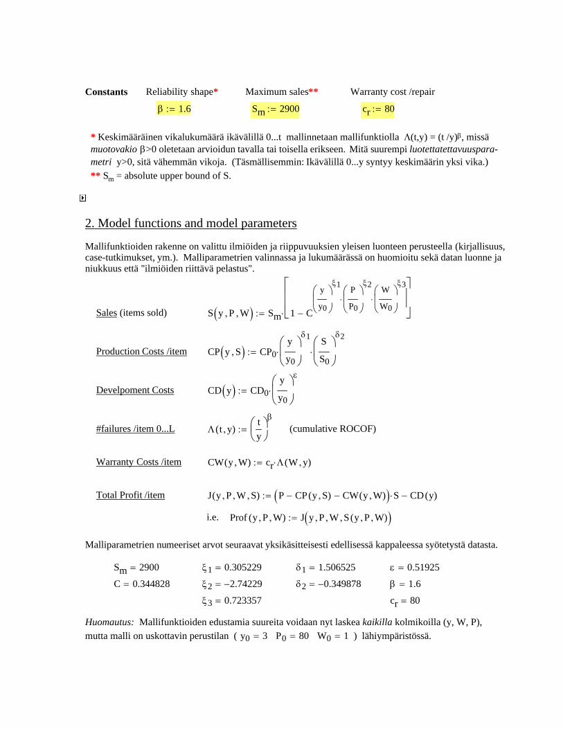
(cumulative ROCOF)
Warranty Costs /item CW y W,( ) cr Λ W y,( )⋅:=
Total Profit /item J y P, W, S,( ) P CP y S,( )− CW y W,( )−( ) S⋅ CD y( )−:=
i.e. Prof y P, W,( ) J y P, W, S y P, W,( ),( ):=
Malliparametrien numeeriset arvot seuraavat yksikäsitteisesti edellisessä kappaleessa syötetystä datasta.
Sm 2900= ξ1 0.305229= δ1 1.506525= ε 0.51925=
C 0.344828= ξ2 2.74229−= δ2 0.349878−= β 1.6=
ξ3 0.723357= cr 80=
Huomautus: Mallifunktioiden edustamia suureita voidaan nyt laskea kaikilla kolmikoilla (y, W, P), mutta malli on uskottavin perustilan ( y0 3= P0 80= W0 1= ) lähiympäristössä.
Constants Reliability shape* Maximum sales** Warranty cost /repair
β 1.6:= Sm 2900:= cr 80:=
* Keskimääräinen vikalukumäärä ikävälillä 0...t mallinnetaan mallifunktiolla Λ(t,y) = (t /y)β, missä muotovakio β>0 oletetaan arvioidun tavalla tai toisella erikseen. Mitä suurempi luotettatettavuuspara- metri y>0, sitä vähemmän vikoja. (Täsmällisemmin: Ikävälillä 0...y syntyy keskimäärin yksi vika.)** Sm = absolute upper bound of S.
2. Model functions and model parameters
Mallifunktioiden rakenne on valittu ilmiöiden ja riippuvuuksien yleisen luonteen perusteella (kirjallisuus, case-tutkimukset, ym.). Malliparametrien valinnassa ja lukumäärässä on huomioitu sekä datan luonne ja niukkuus että "ilmiöiden riittävä pelastus".
Sales (items sold) S y P, W,( ) Sm 1 C
y
y0
⎛⎜⎝
⎞⎟⎠
ξ1 P
P0
⎛⎜⎝
⎞⎟⎠
ξ2
⋅W
W0
⎛⎜⎝
⎞⎟⎠
ξ3
⋅
−
⎡⎢⎢⎣
⎤⎥⎥⎦⋅:=
Production Costs /item CP y S,( ) CP0y
y0
⎛⎜⎝
⎞⎟⎠
δ1
⋅S
S0
⎛⎜⎝
⎞⎟⎠
δ2
⋅:=
Develpoment Costs CD y( ) CD0y
y0
⎛⎜⎝
⎞⎟⎠
ε
⋅:=
#failures /item 0...L Λ t y,( )ty⎛⎜⎝⎞⎟⎠
β:=
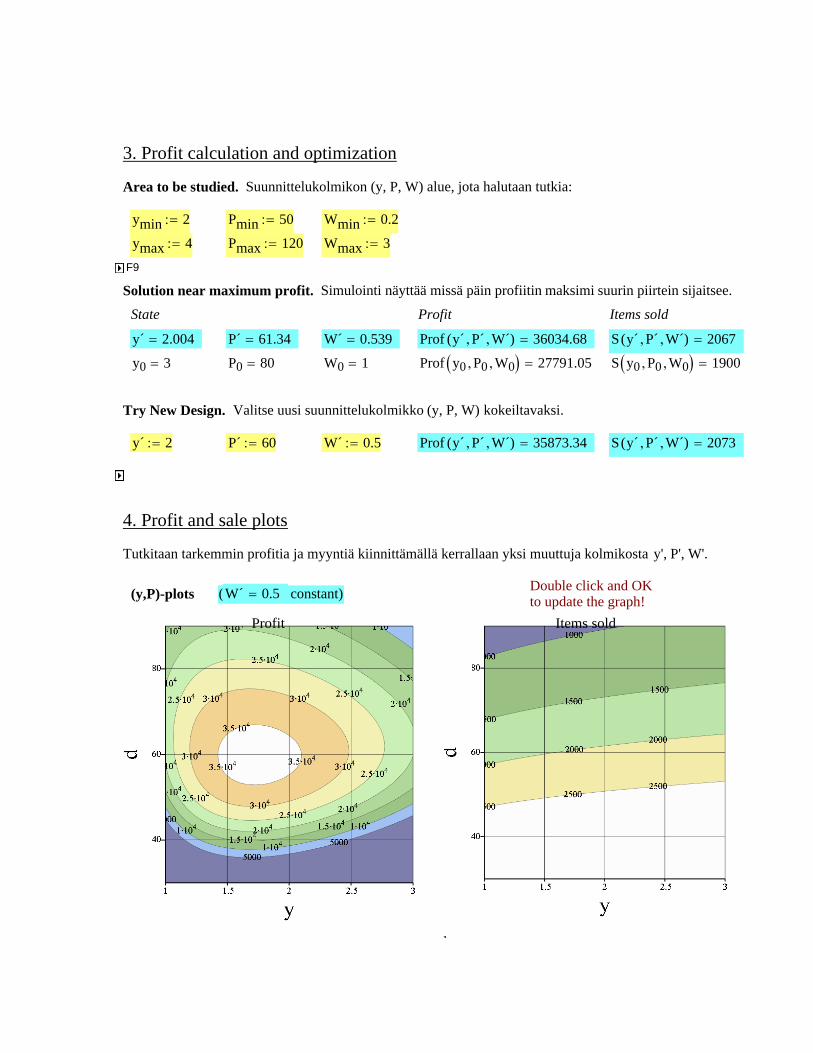
P0 80= W0 1= Prof y0 P0, W0,( ) 27791.05= S y0 P0, W0,( ) 1900=
Try New Design. Valitse uusi suunnittelukolmikko (y, P, W) kokeiltavaksi.
y´ 2:= P´ 60:= W´ 0.5:= Prof y´ P´, W´,( ) 35873.34= S y´ P´, W´,( ) 2073=
4. Profit and sale plots
Tutkitaan tarkemmin profitia ja myyntiä kiinnittämällä kerrallaan yksi muuttuja kolmikosta y', P', W'.
Double click and OK to update the graph!(y,P)-plots (W´ 0.5= constant)
Profit Items sold
b
3. Profit calculation and optimization
Area to be studied. Suunnittelukolmikon (y, P, W) alue, jota halutaan tutkia:
ymin 2:= Pmin 50:= Wmin 0.2:=
ymax 4:= Pmax 120:= Wmax 3:=
F9
Solution near maximum profit. Simulointi näyttää missä päin profiitin maksimi suurin piirtein sijaitsee.
State Profit Items sold
y´ 2.004= P´ 61.34= W´ 0.539= Prof y´ P´, W´,( ) 36034.68= S y´ P´, W´,( ) 2067=
y0 3=
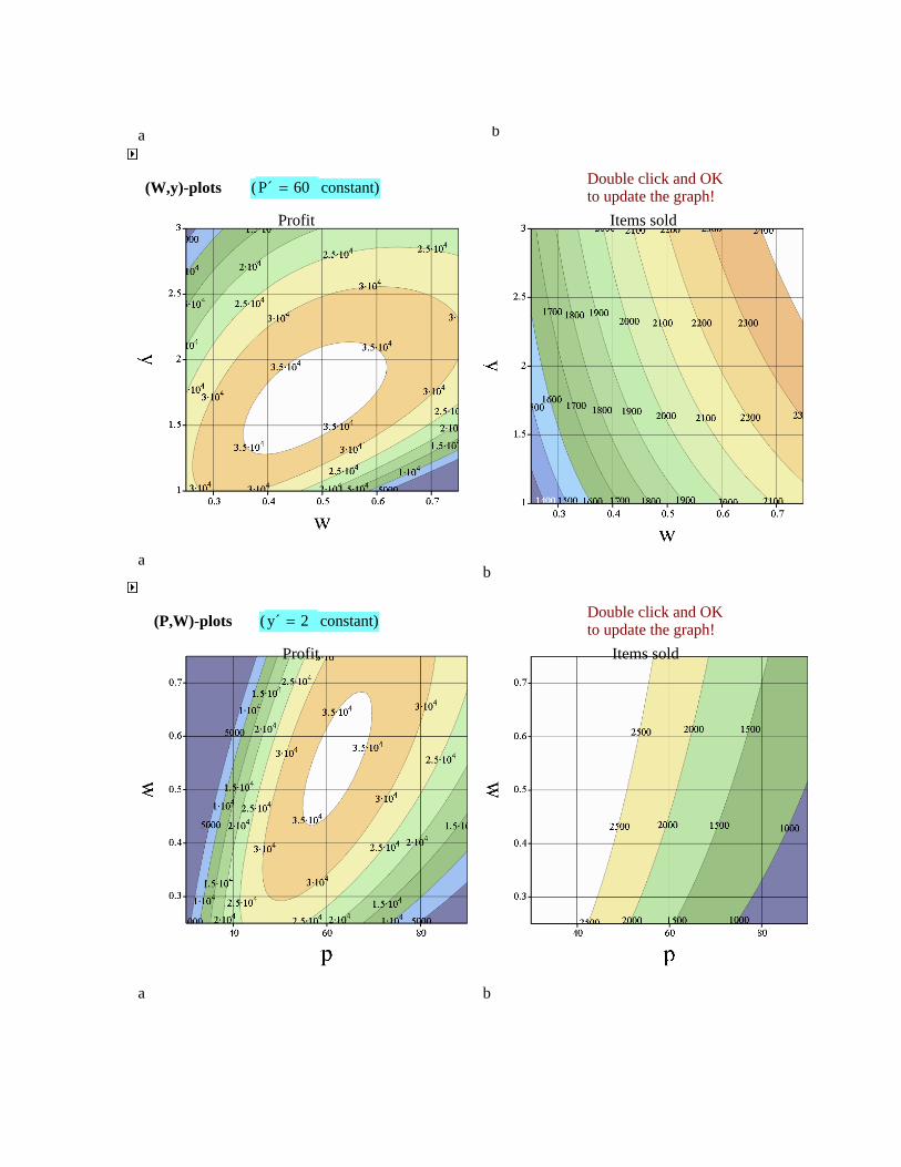
a b
Double click and OK to update the graph!(W,y)-plots (P´ 60= constant)
Profit
a
Items sold
b
Double click and OK to update the graph!(P,W)-plots (y´ 2= constant)
Profit
a
Items sold
b
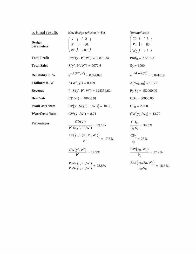
P0 S0⋅ 152000.00=
DevCosts CD y´( ) 48608.91= CD0 60000.00=
ProdCosts /item CP y´ S y´ P´, W´,( ),( ) 10.53= CP0 20.00=
WarrCosts /item CW y´ W´,( ) 8.71= CW y0 W0,( ) 13.79=
Percentages CD y´( )
P´ S y´ P´, W´,( )⋅39.1%=
CD0P0 S0⋅
39.5%=
CP y´ S y´ P´, W´,( ),( )P´
17.6%=CP0P0
25%=
CW y´ W´,( )P´
14.5%=CW y0 W0,( )
P017.2%=
Prof y´ P´, W´,( )P´ S y´ P´, W´,( )⋅
28.8%=Prof y0 P0, W0,( )
P0 S0⋅18.3%=
5. Final results New design (chosen in §3) Nominal state
Design parameters
y´
P´
W´
⎛⎜⎜⎝
⎞⎟⎟⎠
2
60
0.5
⎛⎜⎜⎝
⎞⎟⎟⎠
=
y0
P0
W0
⎛⎜⎜⎜⎝
⎞⎟⎟⎟⎠
3
80
1
⎛⎜⎜⎝
⎞⎟⎟⎠
=
Total Profit Prof y´ P´, W´,( ) 35873.34= Prof0 27791.05=
Total Sales S y´ P´, W´,( ) 2072.6= S0 1900=
Reliability 0...W e Λ W´ y´,( )− 0.896893= eΛ W0 y0,( )−
0.841619=
# failures 0...W Λ W´ y´,( ) 0.109= Λ W0 y0,( ) 0.172=
Revenue P´ S y´ P´, W´,( )⋅ 124354.62=
Muissa sarakkeissa arvioidaan neljä muuta lähellä perustilaa olevaa ja mahdollista systeemin tilaa. Tässä ollaan asiantuntijoiden arvion ja/tai esitutkimuksen varassa.
Seuraavan taulukon ensimmäisessä sarakkeessa arvioidaan sovelluskohteen eli systeemin perustila, eli perusnelikkö F0, U0, P0, W0 ja sitä vastaavien perussuureiden S, PrC, arvot. Perustila voi tarkoittaa esimerkiksi vanhaa kohdetta, joka tunnetaan hyvin, ja joka nyt toimii muutossuunnitelmassa "origona".
DeC DeCm≥( )DeCm 2:=Minimum Design & Development Cost /itemPrC PrCm≥( )PrCm 2:=Minimum Production & Installation Cost /itemS Sm<( )Sm 36:=Maximum Sales (items sold)
Constants
Time unit e.g. days. Cost unit, e.g. euro 10⋅ n.
L 5475=L 15 365⋅:=Life of item (time)
Tarkasteltavaksi voidaan valita mikä tahansa kokonaisuus, esim. tietty markkinajakso tai tietty tuote-erää.
1. Basic quantities, dependences, and constants
Syötöt keltaisella!
Tämä metamalli muistuttaa mallia QuickModel siinä että se on yhden tuotteen staattinen luotettavuus-, takuu-, kustannus-, myynti- ja profiittimalli, mutta se sisältää paljon uusia piirteitä ja on dynaamisempi kuin QuickModel.
Suunnittelumuuttujat, joiden avulla mallinnetaan muut perussuureet, ovat nyt
F # failures /item during 0...L U unavailability time /failure P sale price /item W warranty period 0...W (0 W≤ L< ),
missä L on tuoteyksilön oleellisen eliniän pituus (aika). Perusssuureita ja riippuvuuksia mallinnetaan edelleen tietyn perustilan (origon) lähiympäristössä, mutta nyt kompleksisemmilla mallifunktioilla. Epäkäytettävyysajan U vaikutus myyntiin ja myyntiä edeltäviin kustannuksiin voidaan mallintaa, ja PM-kustannukset ja vikojen aiheuttamat FR-kustannukset voivat riippua muuttujista F ja U, vastaavasti. Tärkeä lisäalue on takuu- ja huoltosopimuskehys, jossa voidaan mallintaa sopimuksien aikavälit ja valmistajan kustannusvastuut. Tätä varten täytyy mallintaa myös PM-kustannusten ja vikataipumuksen kumulatiiviset profiilit.
Mallin avulla voi tarkastella erityisesti myynnin, koko profiitin ja tuoteyksilön profiitin käyttäytymistä suunnittelumuuttujien funktioina, sekä löytää optimaalisia suunnitteluratkaisuja eri näkökulmista katsoen.Kun ratkaisu on kiinnitetty, saadaan tuloksina vielä valmistajan kumulatiiviset takuu- ja huolto- kustannukset eriteltynä PM:n ja FR:n mukaan, sekä kumulatiivinen profiitti /tuoteyksilö.
Comments: [email protected] Optimization
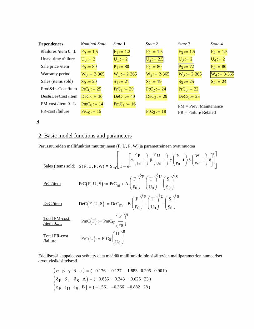
FR-cost /failure PM = Prev. Maintenance FR = Failure Related
PmC1 16:=PmC0 14:=PM-cost /item 0...L
DeC3 25:=DeC2 29:=DeC1 40:=DeC0 30:=Des&DevCost /itemPrC3 22:=PrC2 24:=PrC1 29:=PrC0 25:=Prod&InsCost /item
S4 24:=S3 25:=
α β γ δ ε( ) 0.176− 0.137− 1.883− 0.295 0.901( )=
δF δU δS A( ) 0.856− 0.343− 0.626− 23( )=
εF εU εS B( ) 1.561− 0.366− 0.882− 28( )=
Edellisessä kappaleessa syötetty data määrää mallifunktioihin sisältyvien malliparametrien numeeriset arvot yksikäsitteisesti.
FrC U( ) FrC0U
U0
⎛⎜⎝
⎞⎟⎠
θ
⋅:=Total FR-cost /failure
PmC F( ) PmC0F
F0
⎛⎜⎝
⎞⎟⎠
η
⋅:=Total PM-cost /item 0...L
DeC F U, S,( ) DeCm BF
F0
⎛⎜⎝
⎞⎟⎠
εF
⋅U
U0
⎛⎜⎝
⎞⎟⎠
εU
⋅S
S0
⎛⎜⎝
⎞⎟⎠
εS
⋅+:=DeC /item
PrC F U, S,( ) PrCm AF
F0
⎛⎜⎝
⎞⎟⎠
δF
⋅U
U0
⎛⎜⎝
⎞⎟⎠
δU
⋅S
S0
⎛⎜⎝
⎞⎟⎠
δS
⋅+:=PrC /item
S F U, P, W,( ) Sm 1 eα
F
F01−
⎛⎜⎝
⎞⎟⎠
⋅ βU
U01−
⎛⎜⎝
⎞⎟⎠
⋅+ γP
P01−
⎛⎜⎝
⎞⎟⎠
⋅+ δW
W01−
⎛⎜⎝
⎞⎟⎠
⋅+ ε+⎡⎢⎣
⎤⎥⎦
2
−
⎡⎢⎢⎣
⎤⎥⎥⎦⋅=Sales (items sold)
Perussuureiden mallifunktiot muuttujineen (F, U, P, W) ja parametreineen ovat muotoa
2. Basic model functions and parameters
FrC2 18:=FrC0 15:=
U3 2:=U2 2.5:=U1 2:=U0 2:=Unav. time /failureF4 1.5:=F3 1.5:=F2 1.5:=F1 1.2:=F0 1.5:=#failures /item 0...L
State 4State 3State 2State 1Nominal StateDependences
S2 19:=S1 21:=S0 20:=Sales (items sold)W4 3 365⋅:=W3 2 365⋅:=W2 2 365⋅:=W1 2 365⋅:=W0 2 365⋅:=Warranty periodP4 80:=P3 72:=P2 80:=P1 80:=P0 80:=Sale price /item
U4 2:=
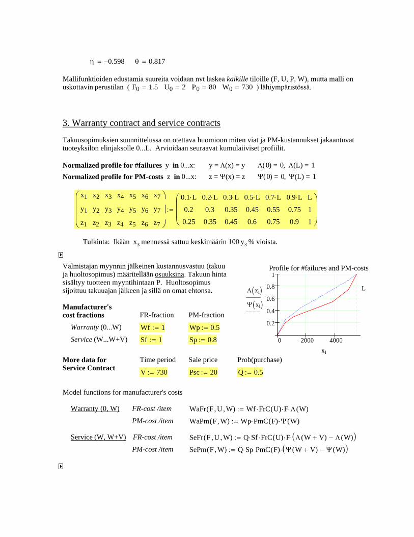
Sp 0.8:=
More data for Service Contract
Time period Sale price Prob(purchase)
V 730:= Psc 20:= Q 0.5:=
Model functions for manufacturer's costs
Warranty (0, W) FR-cost /item WaFr F U, W,( ) Wf FrC U( )⋅ F⋅ Λ W( )⋅:=
PM-cost /item WaPm F W,( ) Wp PmC F( )⋅ Ψ W( )⋅:=
Service (W, W+V) FR-cost /item SeFr F U, W,( ) Q Sf⋅ FrC U( )⋅ F⋅ Λ W V+( ) Λ W( )−( )⋅:=
PM-cost /item SePm F W,( ) Q Sp⋅ PmC F( )⋅ Ψ W V+( ) Ψ W( )−( )⋅:=
η 0.598−= θ 0.817=
Mallifunktioiden edustamia suureita voidaan nyt laskea kaikille tiloille (F, U, P, W), mutta malli on uskottavin perustilan ( F0 1.5= U0 2= P0 80= W0 730= ) lähiympäristössä.
3. Warranty contract and service contracts
Takuusopimuksien suunnittelussa on otettava huomioon miten viat ja PM-kustannukset jakaantuvat tuoteyksilön elinjaksolle 0...L. Arvioidaan seuraavat kumulaiiviset profiilit.
Normalized profile for #failures y in 0...x: y = Λ(x) = y Λ(0) = 0, Λ(L) = 1
Normalized profile for PM-costs z in 0...x: z = Ψ(x) = z Ψ(0) = 0, Ψ(L) = 1
x1
y1
z1
x2
y2
z2
x3
y3
z3
x4
y4
z4
x5
y5
z5
x6
y6
z6
x7
y7
z7
⎛⎜⎜⎜⎝
⎞⎟⎟⎟⎠
0.1 L⋅
0.2
0.25
0.2 L⋅
0.3
0.35
0.3 L⋅
0.35
0.45
0.5 L⋅
0.45
0.6
0.7 L⋅
0.55
0.75
0.9 L⋅
0.75
0.9
L
1
1
⎛⎜⎜⎝
⎞⎟⎟⎠
:=
Tulkinta: Ikään x3 mennessä sattuu keskimäärin 100 y3 % vioista.
0 2000 4000
0.2
0.4
0.6
0.8
1Profile for #failures and PM-costs
Λ xi( )Ψ xi( )
L
xi
Valmistajan myynnin jälkeinen kustannusvastuu (takuu ja huoltosopimus) määritellään osuuksina. Takuun hinta sisältyy tuotteen myyntihintaan P. Huoltosopimus sijoittuu takuuajan jälkeen ja sillä on omat ehtonsa.
Manufacturer'scost fractions FR-fraction PM-fraction
Warranty (0...W) Wf 1:= Wp 0.5:=
Service (W...W+V) Sf 1:=
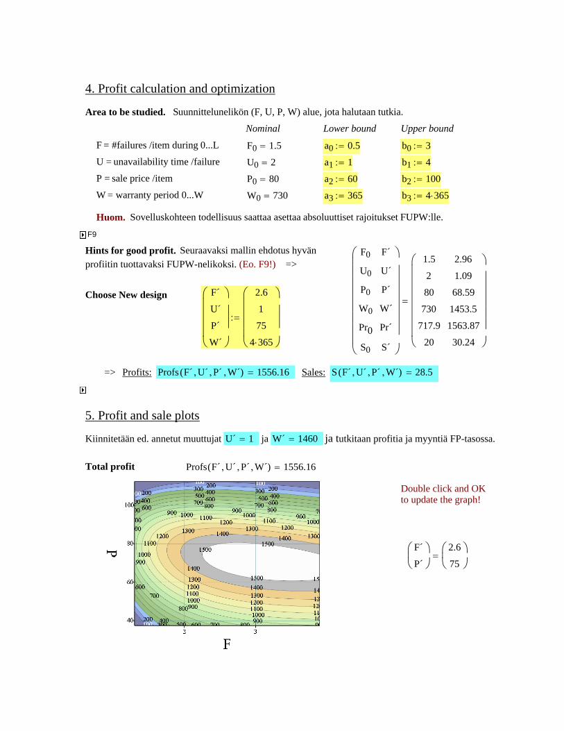
F´
P´⎛⎜⎝
⎞⎟⎠
2.6
75⎛⎜⎝
⎞⎟⎠
=
Double click and OK to update the graph!
Profs F´ U´, P´, W´,( ) 1556.16=Total profit
Kiinnitetään ed. annetut muuttujat U´ 1= ja W´ 1460= ja tutkitaan profitia ja myyntiä FP-tasossa.
5. Profit and sale plots
=> Profits: Profs F´ U´, P´, W´,( ) 1556.16= Sales: S F´ U´, P´, W´,( ) 28.5=
F´
U´
P´
W´
⎛⎜⎜⎜⎜⎝
⎞⎟⎟⎟⎟⎠
2.6
1
75
4 365⋅
⎛⎜⎜⎜⎜⎝
⎞⎟⎟⎟⎟⎠
:=
F0
U0
P0
W0
Pr0
S0
F´
U´
P´
W´
Pr´
S´
⎛⎜⎜⎜⎜⎜⎜⎜⎜⎝
⎞⎟⎟⎟⎟⎟⎟⎟⎟⎠
1.5
2
80
730
717.9
20
2.96
1.09
68.59
1453.5
1563.87
30.24
⎛⎜⎜⎜⎜⎜⎜⎜⎝
⎞⎟⎟⎟⎟⎟⎟⎟⎠
=Choose New design
Hints for good profit. Seuraavaksi mallin ehdotus hyvän profiitin tuottavaksi FUPW-nelikoksi. (Eo. F9!) =>
F9
Huom. Sovelluskohteen todellisuus saattaa asettaa absoluuttiset rajoitukset FUPW:lle.
b3 4 365⋅:=
4. Profit calculation and optimization
Area to be studied. Suunnittelunelikön (F, U, P, W) alue, jota halutaan tutkia.
Nominal Lower bound Upper bound
F = #failures /item during 0...L
U = unavailability time /failure
P = sale price /item
W = warranty period 0...W
F0 1.5= a0 0.5:= b0 3:=
U0 2= a1 1:= b1 4:=
P0 80= a2 60:= b2 100:=
W0 730= a3 365:=

P0 80.00=P´ 75.00=Price (incl.warr) U0 2=U´ 1=Unav. time /failureF0 1.5=F´ 2.6=Failures /item
Nominal designNew design6. Results
HUOM Voi palata mihin tahansa aiempaan keltaiseen kohtaan ja muuttaa syöttöä.
F´
P´⎛⎜⎝
⎞⎟⎠
2.6
75⎛⎜⎝
⎞⎟⎠
=
S F´ U´, P´, W´,( ) 28.5=# items sold
F´
P´⎛⎜⎝
⎞⎟⎠
2.6
75⎛⎜⎝
⎞⎟⎠
=
S F´ U´, P´, W´,( ) 30.4=S F´ U´, P´, W´,( ) 30.4=
ProfPro F´ U´, P´, W´,( ) 35.75=Profit /item (without service contract)
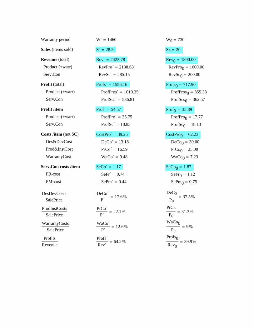
SeFr´ 0.74=FR-costSeCo0 1.87=SeCo´ 1.17=Serv.Con costs /item
WaCo0 7.23=WaCo´ 9.48=WarrantyCost PrCo0 25.00=PrCo´ 16.59=Prod&InstCost DeCo0 30.00=DeCo´ 13.18=Des&DevCost
CostPro0 62.23=CostPro´ 39.25=Costs /item (not SC)
Profs0Rev0
39.9%=Profs´Rev´
64.2%=Profits
Revenue
WaCo0P0
9%=WaCo´
P´12.6%=
WarrantyCostsSalePrice
PrC0P0
31.3%=PrCo´
P´22.1%=
ProdInstCostsSalePrice
DeC0P0
37.5%=DeCo´
P´17.6%=
DesDevCostsSalePrice
SePm0 0.75=SePm´ 0.44=PM-costSeFr0 1.12=
Profit (total)
RevSc0 200.00=RevSc´ 285.15=Serv.ConRevPro0 1600.00=RevPro´ 2138.63=Product (+warr)
Rev0 1800.00=Rev´ 2423.78=Revenue (total)
S0 20=S´ 28.5=Sales (items sold)
W0 730=W´ 1460=Warranty period
ProfSc0 18.13=ProfSc´ 18.83=Serv.ConProfPro0 17.77=ProfPro´ 35.75=Product (+warr)
Prof0 35.89=Prof´ 54.57=Profit /item
ProfScs0 362.57=ProfScs´ 536.81=Serv.ConProfPros0 355.33=ProfPros´ 1019.35=Product (+warr)
Profs0 717.90=Profs´ 1556.16=
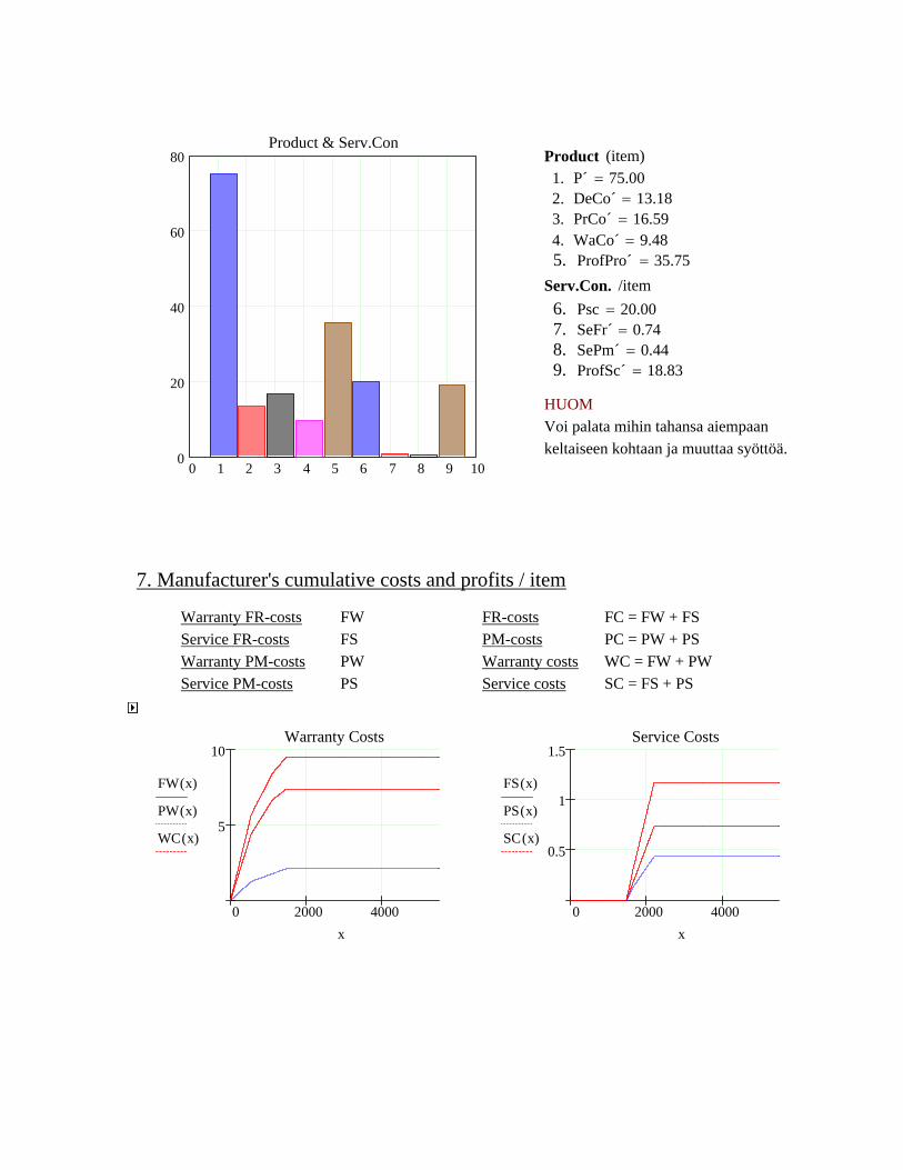
0 1 2 3 4 5 6 7 8 9 100
20
40
60
80Product & Serv.Con
Product (item) 1. P´ 75.00= 2. DeCo´ 13.18= 3. PrCo´ 16.59= 4. WaCo´ 9.48= 5. ProfPro´ 35.75= Serv.Con. /item 6. Psc 20.00= 7. SeFr´ 0.74= 8. SePm´ 0.44= 9. ProfSc´ 18.83=
HUOM Voi palata mihin tahansa aiempaan keltaiseen kohtaan ja muuttaa syöttöä.
7. Manufacturer's cumulative costs and profits / item
Warranty FR-costs FW Service FR-costs FS Warranty PM-costs PW Service PM-costs PS
FR-costs FC = FW + FS PM-costs PC = PW + PS Warranty costs WC = FW + PW Service costs SC = FS + PS
0 2000 4000
5
10Warranty Costs
FW x( )
PW x( )
WC x( )
x0 2000 4000
0.5
1
1.5Service Costs
FS x( )
PS x( )
SC x( )
x

0 2000 4000
5
10FR costs
FW x( )
FS x( )
FC x( )
x0 2000 4000
1
2
3PM costs
PW x( )
PS x( )
PC x( )
x
Time before sale (DeCo & PrCo) D 2 365⋅:= x D− D− 0.001 L⋅+, L..:=
Manufacturer'scumulative profit
Profit x( ) D− x< 0≤( ) DeCo´− PrCo´−( )⋅xD
1+⎛⎜⎝
⎞⎟⎠
⋅
x 0≥( ) P´ DeCo´− PrCo´−( )⋅ WC x( )− SC x( )−+
...
Q Psc⋅ 0 x W´−< V≤( )x W´−
V⋅ x W´ V+>( )+⎡⎢
⎣⎤⎥⎦
⋅+
...
:=
0 2000 4000 6000
40
20
20
40
60
Profit x( )
W´ W´ V+
x
Asiakas maksaa tuotteen kerralla ja huoltosopimuksen tasaisesti W...W+V
HUOM Voi palata mihin tahansa aiempaan keltaiseen kohtaan ja muuttaa syöttöä.

D0
1
0.2 L⋅2
0.4 L⋅3
0.6 L⋅3
0.8 L⋅1
⎛⎜⎝
⎞⎟⎠
T:= PM-kustannusten suhteel-
linen jakautuminen 0..LProportional profile for PM costs /item 0..L
Pm 21.5:= siinä tapauksessa että valmistaja tekisi "kaiken"
PM costs /item 0..L (ry)
Ennakohuolto (PM) tarkoittaa tässä kaikkea sellaista kunnossapitoa, jonka tapahtumahetket ja kustannukset ovat (myyntihetkellä) melko tarkasti tiedossa.
(ky = käyttömääräyksikkö)L 5400:=Life of item (ky) valmistajan kannalta kiinnostava jakso 0..L
(ry = rahayksikkö)Pre 10.6:=Pre-costs /item (ry)Jos ei oteta huomioon,niin Pre = 0.
Arvioi valmistajan kustannukset yhteensä ennen käyttöönottoa (can include design, development, production, installation, etc.).
1. Pre-costs and PM costs (constants for item)
Syötöt keltaisella!
Tämän metamallin keskeiset ainekset ovat käyttövarmuus, takuu- ja huoltosopimukset, kustannukset, hinnoittelu, myynti, riskit, profiitit. Erityisenä vahvuutena on kustannus- ja profiitti- riskien yksityiskohtainen stokastinen mallinnus. Perusnäkökulma on valmistajan, mutta älykkäillä tulkinnoilla malli palvelee myös muita näkökulmia.
Valitaan tarkasteltavaksi tuoteyksilön elinjakso vähintään sen pituisena kuin se valmistajaa voi kiinnostaa takuu- ja huoltosopimuksia ajatellen. Yllätyksettömät kulut kuten valmistus- ja asennuskustannukset sekä ennakkohuollon kustannukset (PM) käsitellään ilman satunnaisuutta, jälkimmäisiä myös profiloituna elinjaksolle. Yllättävät "viat" voidaan jakaa 4 eri tyyppiin, ja jokaisen tyypin esiintymisen riippuvuus iästä mallinnetaan. Tuoteyksilön vikojen lukumäärät eri ikäväleillä ja FR(failure-related)-kustannukset mallinnetaan satunnaissuureina ja simuloidaan.
Takuu- ja huoltosopimuksille (1+3 kpl) malli tarjoaa yhtenäisen ja melko yleisen kehyksen, johon monet käytännössä esiintyvät sopimustyypit voidaan sovittaa pienellä esilaskennalla. Tämä merkitsee esimerkiksi, että valmistaja voi eksperimentoida minkälaisiin kustannusjakaumiin, profiitteihin ja siten taloudellisiin riskeihin erilaiset takuu- tai huoltosopimukset tai hinnoittelu johtavat. Tarkastelu voidaan tehdä myös sopimuskohtaisesti.
Lopuksi koko tarkastelu laajenee tuoteyksilöstä tuote-eriin, kun myös myyntimäärä mallinnetaan stokastisena. Oppimis- ja demonstraatiomielessä voi myös simuloida satunnaisten tuoteyksilöiden historiat (valmistajan tulot, menot, profiitit).
Comments: [email protected] Analysis
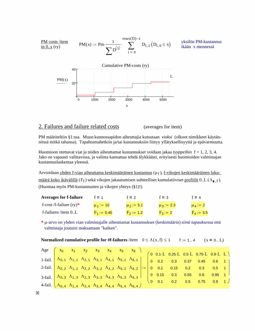
4-fail.
3-fail.
x0
Λ0 1,
Λ0 2,
Λ0 3,
Λ0 4,
x1
Λ1 1,
Λ1 2,
Λ1 3,
Λ1 4,
x2
Λ2 1,
Λ2 2,
Λ2 3,
Λ2 4,
x3
Λ3 1,
Λ3 2,
Λ3 3,
Λ3 4,
x4
Λ4 1,
Λ4 2,
Λ4 3,
Λ4 4,
x5
Λ5 1,
Λ5 2,
Λ5 3,
Λ5 4,
x6
Λ6 1,
Λ6 2,
Λ6 3,
Λ6 4,
⎛⎜⎜⎜⎜⎜⎜⎝
⎞⎟⎟⎟⎟⎟⎟⎠
0
0
0
0
0
0.1 L⋅0.2
0.1
0.15
0.1
0.25 L⋅0.3
0.15
0.3
0.2
0.5 L⋅0.37
0.2
0.55
0.5
0.75 L⋅0.45
0.3
0.8
0.75
0.9 L⋅0.6
0.5
0.95
0.9
L1
1
1
1
⎛⎜⎜⎜⎜⎜⎝
⎞⎟⎟⎟⎟⎟⎠
:=2-fail.
1-fail.
Age
x 0= L..( )f 1 4..:=Normalized cumulative profile for #f-failures /item 0 Λ x f,( )≤ 1≤
* μ-arvo on yhden vian valmistajalle aiheuttamat kustannukset (keskimäärin) siinä tapauksessa että valmistaja joutuisi maksamaan "kaiken".
F4 3.5:=F3 2:=F2 1.2:=F1 0.45:= f-failures /item 0..Lμ4 2:=μ3 2.3:=μ2 5.1:=μ1 10:= f-cost /f-failure (ry)*f 4=f 3=f 2=f 1=Averages for f-failure
PM määriteltiin §1:ssa. Muun kunnossapidon aiheuttajia kutsutaan vioksi (olkoot nimikkeet käytän- nössä mitkä tahansa). Tapahtumahetkiin ja/tai kustannuksiin liittyy yllätyksellisyyttä ja epävarmuutta.
Huomioon otettavat viat ja niiden aiheuttamat kustannukset voidaan jakaa tyyppeihin f = 1, 2, 3, 4. Jako on vapaasti valittavissa, ja valinta kannattaa tehdä älykkäästi, erityisesti huomioiden valmistajan kustannuslaskentaa yleensä.
Arvioidaan yhden f-vian aiheuttama keskimääräinen kustannus (μf ), f-vikojen keskimääräinen luku- määrä koko ikävälillä (Ff ) sekä vikojen jakautumisen suhteelliset kumulatiiviset profiilit 0..L (Λ f, ). (Huomaa myös PM-kustannusten ja vikojen yhteys (§1)!)
2. Failures and failure related costs (averages for item)
0 1000 2000 3000 4000 5000
20
40Cumulative PM-costs (ry)
PM x( )L
x
PM x( ) Pm1
D 1⟨ ⟩∑⋅
0
rows D( ) 1−
i
Di 1, Di 0, x≤( )⋅∑=
⋅:= yksilön PM-kustannus ikään x mennessä
PM costs /item in 0..x (ry)
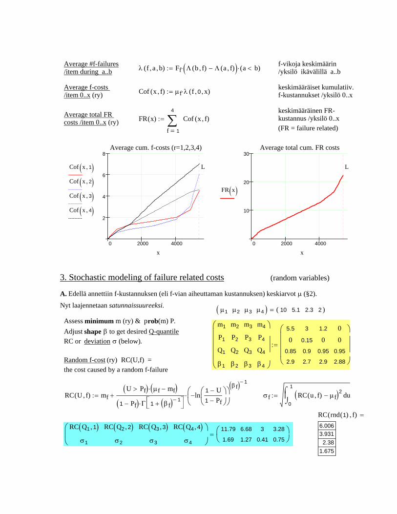
RC Q1 1,( )σ1
RC Q2 2,( )σ2
RC Q3 3,( )σ3
RC Q4 4,( )σ4
⎛⎜⎝
⎞⎟⎠
11.79
1.69
6.68
1.27
3
0.41
3.28
0.75⎛⎜⎝
⎞⎟⎠=
RC rnd 1( ) f,( )6.0063.9312.38
1.675
=
σf0
1
uRC u f,( ) μf−( )2⌠⎮⌡
d:=RC U f,( ) mfU Pf>( ) μf mf−( )⋅
1 Pf−( ) Γ 1 βf( ) 1−+⎡⎣ ⎤⎦⋅ln
1 U−1 Pf−⎛⎜⎝
⎞⎟⎠
−⎛⎜⎝
⎞⎟⎠
βf( ) 1−
⋅+:=
Random f-cost (ry) RC(U,f) = the cost caused by a random f-failure
m1
P1
Q1
β1
m2
P2
Q2
β2
m3
P3
Q3
β3
m4
P4
Q4
β4
⎛⎜⎜⎜⎜⎝
⎞⎟⎟⎟⎟⎠
5.5
00.85
2.9
3
0.15
0.9
2.7
1.2
00.95
2.9
0
00.95
2.88
⎛⎜⎜⎜⎜⎝
⎞⎟⎟⎟⎟⎠
:=
Assess minimum m (ry) & prob(m) P. Adjust shape β to get desired Q-quantile RC or deviation σ (below).
μ1 μ2 μ3 μ4( ) 10 5.1 2.3 2( )=Nyt laajennetaan satunnaissuureeksi.
A. Edellä annettiin f-kustannuksen (eli f-vian aiheuttaman kustannuksen) keskiarvot μ (§2).
3. Stochastic modeling of failure related costs (random variables)
0 2000 4000
10
20
30Average total cum. FR costs
FR x( )
L
x0 2000 4000
2
4
6
8Average cum. f-costs (r=1,2,3,4)
Cof x 1,( )Cof x 2,( )Cof x 3,( )Cof x 4,( )
L
x
FR x( )
1
4
f
Cof x f,( )∑=
:=Average total FR costs /item 0..x (ry)
keskimääräinen FR- kustannus /yksilö 0..x (FR = failure related)
Cof x f,( ) μf λ f 0, x,( )⋅:= keskimääräiset kumulatiiv. f-kustannukset /yksilö 0..x
Average f-costs /item 0..x (ry)
λ f a, b,( ) Ff Λ b f,( ) Λ a f,( )−( )⋅ a b<( )⋅:= f-vikoja keskimäärin /yksilö ikävälillä a..b
Average #f-failures /item during a..b
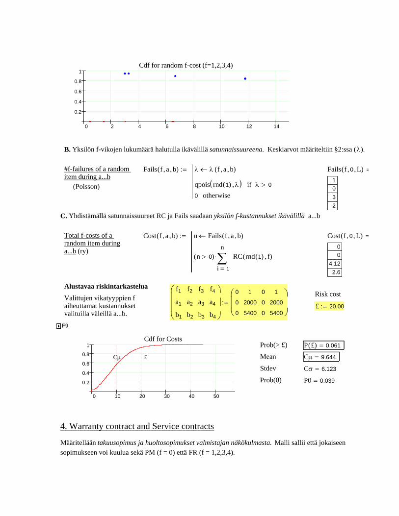
Määritellään takuusopimus ja huoltosopimukset valmistajan näkökulmasta. Malli sallii että jokaiseen sopimukseen voi kuulua sekä PM (f = 0) että FR (f = 1,2,3,4).
4. Warranty contract and Service contracts
P0 0.039=Prob(0)Cσ 6.123=Stdev Cμ 9.644=MeanP £( ) 0.061=Prob(> £)
0 10 20 30 40 50
0.2
0.4
0.6
0.8
1Cdf for Costs
Cμ £
F9
£ 20.00:=
f1
a1
b1
f2
a2
b2
f3
a3
b3
f4
a4
b4
⎛⎜⎜⎜⎝
⎞⎟⎟⎟⎠
0
0
0
1
2000
5400
0
0
0
1
2000
5400
⎛⎜⎜⎝
⎞⎟⎟⎠
:=Risk cost
Alustavaa riskintarkastelua
Valittujen vikatyyppien f
aiheuttamat kustannukset valituilla väleillä a...b.
Cost f 0, L,( )00
4.122.6
=Cost f a, b,( ) n Fails f a, b,( )←
n 0>( )
1
n
i
RC rnd 1( ) f,( )∑=
⋅
:=Total f-costs of a random item duringa...b (ry)
C. Yhdistämällä satunnaissuureet RC ja Fails saadaan yksilön f-kustannukset ikävälillä a...b
Fails f 0, L,( )1032
=Fails f a, b,( ) λ λ f a, b,( )←
qpois rnd 1( ) λ,( ) λ 0>if0 otherwise
:=#f-failures of a random item during a...b (Poisson)
B. Yksilön f-vikojen lukumäärä halutulla ikävälillä satunnaissuureena. Keskiarvot määriteltiin §2:ssa (λ).
0 2 4 6 8 10 12 14
0.2
0.4
0.6
0.8
1Cdf for random f-cost (f=1,2,3,4)

C1 6.78= C2 11.47= C3 3.3=
Constant Cc0 0.5= Cc1 0= Cc2 1.5= Cc3 1=
PM (const.) PM L 0,( ) 0= PM L 1,( ) 6.45= PM L 2,( ) 7.53= PM L 3,( ) 0=
FR mean FR L 0,( ) 2.02= FR L 1,( ) 0.33= FR L 2,( ) 2.45= FR L 3,( ) 2.3=
Risk FR cost £0 10:= £1 3:= £2 7:= £3 4:=
Valmistajan vastuu mallinnetaan suoraan osuuksina kustannuksista (§1-3) eri ikäväleillä.
( as f, ..bs f, ) interval for f-cost in s-contractps f, manufacturer's fraction of f-cost in (as f, ..bs f, )(As .. Bs) interval during which the s-contract is paidCcs manufacturer's constant cost with s-contract
Index symbols Warranty s = 0 Service s = 1, 2, 3 PM cost f = 0 FR cost f = 1, 2, 3, 4
The contracts PM f=1 f=2 f=3 f=4 (= cost types)
Warranty (s=0)
a0 0,
b0 0,
p0 0,
a0 1,
b0 1,
p0 1,
a0 2,
b0 2,
p0 2,
a0 3,
b0 3,
p0 3,
a0 4,
b0 4,
p0 4,
A0
B0
Cc0
⎛⎜⎜⎜⎝
⎞⎟⎟⎟⎠
0
0
0
0
1080
1
0
1080
1
0
0
0
0
0
0
0
0
0.50
⎛⎜⎜⎝
⎞⎟⎟⎠
:=
Service 1 (s=1)
a1 0,
b1 0,
p1 0,
a1 1,
b1 1,
p1 1,
a1 2,
b1 2,
p1 2,
a1 3,
b1 3,
p1 3,
a1 4,
b1 4,
p1 4,
A1
B1
Cc1
⎛⎜⎜⎜⎝
⎞⎟⎟⎟⎠
0
1080
1
0
0
0
1080
3240
0.5
0
0
0
0
0
0
0
3240
0.00
⎛⎜⎜⎝
⎞⎟⎟⎠
:=
Service 2 (s=2)
a2 0,
b2 0,
p2 0,
a2 1,
b2 1,
p2 1,
a2 2,
b2 2,
p2 2,
a2 3,
b2 3,
p2 3,
a2 4,
b2 4,
p2 4,
A2
B2
Cc2
⎛⎜⎜⎜⎝
⎞⎟⎟⎟⎠
1080
5400
0.5
1080
3240
0.2
3240
5400
0.5
0
0
0
0
0
0
0
5400
1.50
⎛⎜⎜⎝
⎞⎟⎟⎠
:=
Service 3 (s=3)
a3 0,
b3 0,
p3 0,
a3 1,
b3 1,
p3 1,
a3 2,
b3 2,
p3 2,
a3 3,
b3 3,
p3 3,
a3 4,
b3 4,
p3 4,
A3
B3
Cc3
⎛⎜⎜⎜⎝
⎞⎟⎟⎟⎠
0
0
0
0
0
0
0
0
0
0
5400
0.5
0
0
0
0
5400
1.00
⎛⎜⎜⎝
⎞⎟⎟⎠
:=
5. Manufacturer's Warranty-Service (WS) costs and FR risks (item)
Lasketaan valmistajan takuu- ja huoltokustannukset. FR-kustannukset saadaan täydellisinä jakaumina, joten voidaan tutkia myös riskejä.
WS costs Warranty Service 1 Service 2 Service 3
Total C0 2.52=
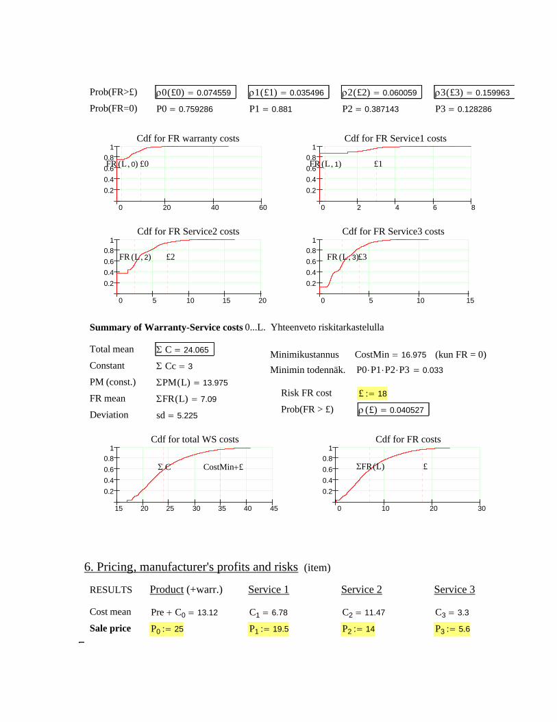
ΣFR L( ) 7.09=Prob(FR > £) ρ £( ) 0.040527=Deviation sd 5.225=
15 20 25 30 35 40 45
0.20.40.60.8
1Cdf for total WS costs
Σ C CostMin £+
0 10 20 30
0.20.40.60.8
1Cdf for FR costs
ΣFR L( ) £
6. Pricing, manufacturer's profits and risks (item)
RESULTS Product (+warr.) Service 1 Service 2 Service 3
Cost mean Pre C0+ 13.12= C1 6.78= C2 11.47= C3 3.3=
Sale price P0 25:= P1 19.5:= P2 14:= P3 5.6:=
Prob(FR>£) ρ0 £0( ) 0.074559= ρ1 £1( ) 0.035496= ρ2 £2( ) 0.060059= ρ3 £3( ) 0.159963=
Prob(FR=0) P0 0.759286= P1 0.881= P2 0.387143= P3 0.128286=
0 20 40 60
0.20.40.60.8
1Cdf for FR warranty costs
FR L 0,( ) £0
0 2 4 6 8
0.20.40.60.8
1Cdf for FR Service1 costs
FR L 1,( ) £1
0 5 10 15 20
0.20.40.60.8
1Cdf for FR Service2 costs
FR L 2,( ) £2
0 5 10 15
0.20.40.60.8
1Cdf for FR Service3 costs
FR L 3,( )£3
Summary of Warranty-Service costs 0...L. Yhteenveto riskitarkastelulla
Total mean Σ C 24.065= Minimikustannus CostMin 16.975= (kun FR = 0)
Minimin todennäk. P0 P1⋅ P2⋅ P3⋅ 0.033=Constant Σ Cc 3=
PM (const.) ΣPM L( ) 13.975=Risk FR cost £ 18:=FR mean

6 8 10 120
0.20.40.60.8
1Cdf for Service1 profit
Pro1£1
10 5 0 50
0.20.40.60.8
1Cdf for Service2 profit
Pro2£2
6 4 2 0 2 40
0.20.40.60.8
1Cdf for Service3 profit
Pro3£3
Total profit and risk analysis Risk profit £ 20:=
0 10 20 30
0.2
0.4
0.6
0.81
Cdf for total profit (item)
Pro£
Prob(< £) ρ £( ) 0.059537=
Profit mean Pro 29.44=
Profit max. Pro 1( ) 36.53=
Prob(max.) P0 P1⋅ P2⋅ P3⋅ 0.033=
7. Modeling the sale of lots
Tähän mennessä on käsitelty yksilöitä. Tarkastellaan nyt useita 'samanlaisia' yksilöitä eli erää. Esimerkki: Erä voi koostua kerralla tai tietyn markkinajakson aikana myytävistä yksilöistä.
Assessing lot size(# items sold)
Bad 6:= Mean 7.5:= Bad Mean< Good<
Good 10:= Pr 0.95:= Pr = Prob (Bad...Good)
Profit mean Pro0 11.88= Pro1 12.72= Pro2 2.53= Pro3 2.3=
Risk profit £0 3:= £1 10.:= £2 1:= £3 0:=
Prob(< £s) ρ0 £0( ) 0.053354= ρ1 £1( ) 0.031772= ρ2 £2( ) 0.238088= ρ3 £3( ) 0.104532=
Profit = max. Pro0 1( ) 13.9= Pro1 1( ) 13.05= Pro2 1( ) 4.97= Pro3 1( ) 4.6=
Prob(max.) P0 0.759286= P1 0.881= P2 0.387143= P3 0.128286=
20 10 0 100
0.20.40.60.8
1Cdf for Prod (+Warr) profit
Pro0£0

Manufacturer's profit balance. Random item (red), average item (blue), lucky item (black).
yT
"Age"
"Failure type"
"Total FR cost"
"Manuf. FR cost"
190
2
6.318
6.318
305
4
0.73
0
1745
4
2.084
0
1844
4
2.613
0
2152
4
1.014
0
3131
2
5.643
2.821
3965
4
2.488
0
4041
3
2.051
1.025
5047
2
5.071
2.535
5094
4
1.481
0
5130
4
2.056
0
⎛⎜⎜⎜⎝
⎞⎟⎟⎟⎠
=
Failure history. (Click & F9 above!)
8. Demo: Failure history and profit balance of a random item
F9
stdev prof( ) 39.2=
mean prof( ) 221.11=
δpr £( ) 0.091=Prob(<£)
50 100 150 200 250 300 350 400
0.2
0.4
0.6
0.8
1Cdf for Profit
mean prof( )£
£ 170:=Risk profit
stdev cost( ) 45.22=
mean cost( ) 259.25=
δco £( ) 0.065=Prob(>£)
100 150 200 250 300 350 400 450 500
0.2
0.4
0.6
0.8
1Cdf for Cost
mean cost( ) £
£ 330:=Risk cost
stdev inc( ) 79.47=
mean inc( ) 480.36=
Income figures
100 200 300 400 500 600 700 800
0.2
0.4
0.6
0.8
1Cdf for Income
Bad Good
N rnd 1( )( ) 7=
( κ 41.025= )N U( ) Znμκ
qgamma U κ,( )⋅←
floor Z( ) rnd 1( ) Z floor Z( )−<( )+
:=Random lot size
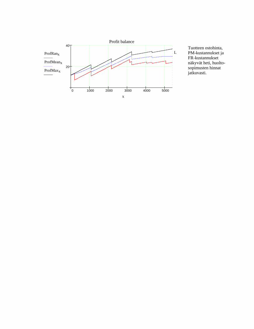
0 1000 2000 3000 4000 5000
20
40Profit balance
ProfRanx
ProfMeanx
ProfMaxx
L
x
Tuotteen ostohinta, PM-kustannukset ja FR-kustannukset näkyvät heti, huolto- sopimusten hinnat jatkuvasti.

Diffusion Model I Comments: [email protected]
Tämä on yhden tuotteen metamalli, jossa suureiden muuttuminen lasketaan diffuusioperiaatteella sekä tuoteyksilön elinaikana että markkinajakson aikana.
Perusmalleilla voidaan määritellä eri vikatyyppien esiintyminen ja niiden aiheuttamat kustannukset (FR), ennakkohuollon kustannukset (PM), valmistuskustannukset, takuusopimus ja huoltosopimus, populaatio, satsaus mainostamiseen, todellinen ja odotettu myyntihinta, asiakastyytyväisyys liittyen hintaan ja vikoihin, ym., ja näiden mahdollinen aika-riippuvuus.
Rakennetaan tietoiseksi tulemisen, ensimmäisen oston ja uudelleenoston ajasta riippuvat "todennäköi- syydet" ottaen myös humioon kuinka mones osto on kyseessä. Säätöparametrit ja rinnakkaiset differenssiyhtälöt ohjaavat markkinatilan ajallista muuttumista, eli erilaisten asiakaslukumäärien (potentiaaliset ostajat, kerran ostaneet, kaksikertaa ostaneet, jne.) kehittymistä.
Tästä diffuusion tuottamasta perusdatasta malli laskee kustannusten, tulojen, profiittien ym. ajallista kehittymistä markkinajaksolla.
Mainittava piirre tämän mallin rakenteessa on sen käännettävyys. Markkinajakson todellisesta datasta voitaisiin kääntäen laskea säätöparametrien arvot.
Syötöt keltaisella!
1. Product's failure tendency* Use such a time unit (tu) that a customer buys at most once item during t...t+1. Example: If a customer buys maximally 1 item/day, then choose (tu) = day, or less!
Useful life of item (tu)* L 500:=
Failure types: f = 1,2,3... (vikatyypit täysin vapaasti valittavissa)
Real average #failures (manufacturer) vms,f = #f-failures in time interval 0...ξs
(Basic reliability, PM, ageing, etc.)
Tolerated average #failures (customer) vcs,f = #f-failures in time interval 0...ξs
(How is this assessed? Inquiries?)
ξ1
vm1 1,
vm1 2,
vm1 3,
vc1 1,
vc1 2,
vc1 3,
ξ2
vm2 1,
vm2 2,
vm2 3,
vc2 1,
vc2 2,
vc2 3,
ξ3
vm3 1,
vm3 2,
vm3 3,
vc3 1,
vc3 2,
vc3 3,
ξ4
vm4 1,
vm4 2,
vm4 3,
vc4 1,
vc4 2,
vc4 3,
ξ5
vm5 1,
vm5 2,
vm5 3,
vc5 1,
vc5 2,
vc5 3,
⎛⎜⎜⎜⎜⎜⎜⎜⎜⎜⎜⎝
⎞⎟⎟⎟⎟⎟⎟⎟⎟⎟⎟⎠
0.05 L⋅0.25
0.05
0.05
0.2
0.2
0.1
0.2 L⋅0.35
0.1
0.1
0.35
0.35
0.2
0.4 L⋅0.4
0.2
0.2
0.4
0.5
0.3
0.7 L⋅0.5
0.7
0.5
0.6
0.9
0.6
L0.7
1.7
1.2
0.8
1.2
0.9
⎛⎜⎜⎜⎜⎜⎜⎜⎜⎝
⎞⎟⎟⎟⎟⎟⎟⎟⎟⎠
:=
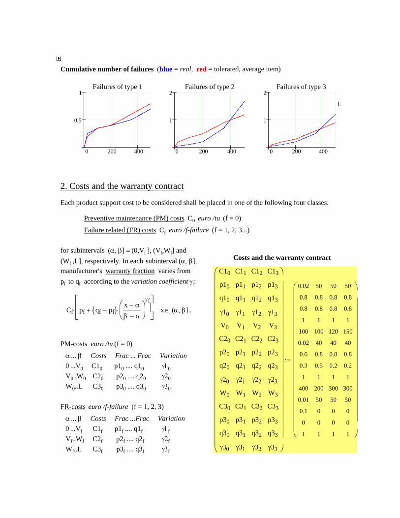
Cumulative number of failures (blue = real, red = tolerated, average item)
0 200 400
0.5
1Failures of type 1
0 200 400
1
2Failures of type 2
0 200 400
1
2Failures of type 3
L
2. Costs and the warranty contract
Each product support cost to be considered shall be placed in one of the following four classes:
Preventive maintenance (PM) costs C0 euro /tu (f = 0)
Failure related (FR) costs Cf euro /f-failure (f = 1, 2, 3...)
for subintervals (α, β] = (0,Vf ], (Vf,Wf] and (Wf ,L], respectively. In each subinterval (α, β],manufacturer's warranty fraction varies from pf to qf according to the variation coefficient γf:
Cf pf qf pf−( ) x α−
β α−⎛⎜⎝
⎞⎟⎠
γf
⋅+⎡⎢⎢⎣
⎤⎥⎥⎦
⋅ x∈ (α, β] .
Costs and the warranty contract
PM-costs euro /tu (f = 0)
α ... β Costs Frac ... Frac Variation 0 ...V0 C10 p10 .... q10 γ10 V0..W0 C20 p20 .... q20 γ20 W0..L C30 p30 .... q30 γ30
C10
p10
q10
γ10
V0
C20
p20
q20
γ20
W0
C30
p30
q30
γ30
C11
p11
q11
γ11
V1
C21
p21
q21
γ21
W1
C31
p31
q31
γ31
C12
p12
q12
γ12
V2
C22
p22
q22
γ22
W2
C32
p32
q32
γ32
C13
p13
q13
γ13
V3
C23
p23
q23
γ23
W3
C33
p33
q33
γ33
⎛⎜⎜⎜⎜⎜⎜⎜⎜⎜⎜⎜⎜⎜⎜⎜⎜⎜⎜⎜⎜⎜⎝
⎞⎟⎟⎟⎟⎟⎟⎟⎟⎟⎟⎟⎟⎟⎟⎟⎟⎟⎟⎟⎟⎟⎠
0.02
0.8
0.8
1
100
0.02
0.6
0.3
1
400
0.01
0.1
0
1
50
0.8
0.8
1
100
40
0.8
0.5
1
200
50
0
0
1
50
0.8
0.8
1
120
40
0.8
0.2
1
300
50
0
0
1
50
0.8
0.8
1
150
40
0.8
0.2
1
300
50
0
0
1
⎛⎜⎜⎜⎜⎜⎜⎜⎜⎜⎜⎜⎜⎜⎜⎜⎜⎜⎝
⎞⎟⎟⎟⎟⎟⎟⎟⎟⎟⎟⎟⎟⎟⎟⎟⎟⎟⎠
:=
FR-costs euro /f-failure (f = 1, 2, 3)
α ... β Costs Frac ...Frac Variation 0 ...Vf C1f p1f .... q1f γ1f Vf..Wf C2f p2f .... q2f γ2f
Wf..L C3f p3f .... q3f γ3f
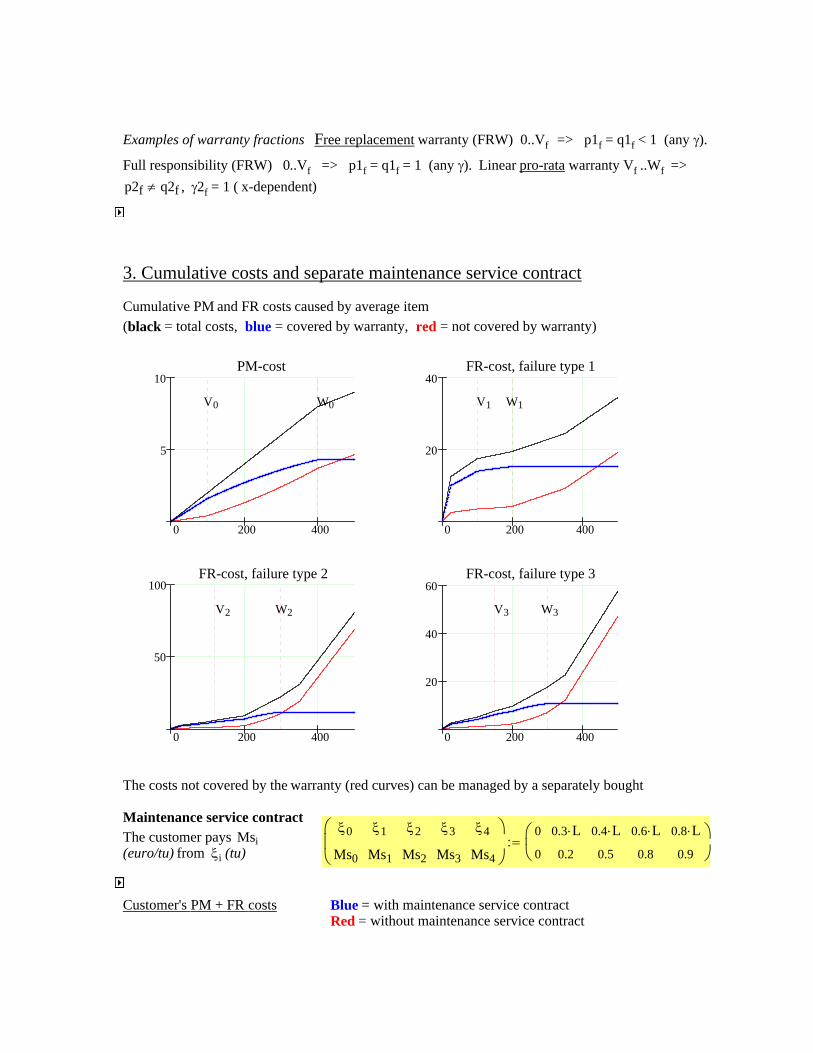
Examples of warranty fractions Free replacement warranty (FRW) 0..Vf => p1f = q1f < 1 (any γ).
Full responsibility (FRW) 0..Vf => p1f = q1f = 1 (any γ). Linear pro-rata warranty Vf ..Wf =>
p2f q2f≠ , γ2f = 1 ( x-dependent)
3. Cumulative costs and separate maintenance service contract
Cumulative PM and FR costs caused by average item (black = total costs, blue = covered by warranty, red = not covered by warranty)
0 200 400
5
10PM-cost
V0 W0
0 200 400
20
40FR-cost, failure type 1
W1V1
0 200 400
50
100FR-cost, failure type 2
W2V2
0 200 400
20
40
60FR-cost, failure type 3
W3V3
The costs not covered by the warranty (red curves) can be managed by a separately bought
Maintenance service contract The customer pays Msi (euro/tu) from ξi (tu)
ξ0
Ms0
ξ1
Ms1
ξ2
Ms2
ξ3
Ms3
ξ4
Ms4
⎛⎜⎝
⎞⎟⎠
0
0
0.3 L⋅0.2
0.4 L⋅0.5
0.6 L⋅0.8
0.8 L⋅0.9
⎛⎜⎝
⎞⎟⎠
:=
Customer's PM + FR costs Blue = with maintenance service contractRed = without maintenance service contract
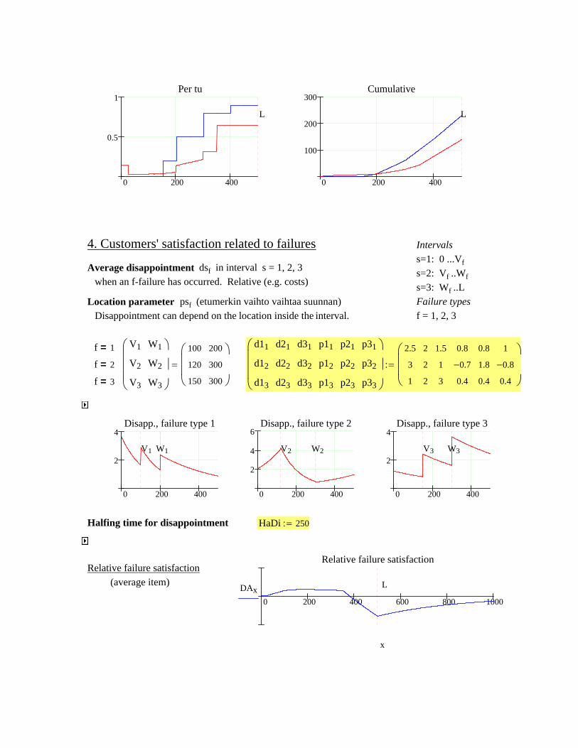
Relative failure satisfaction (average item)
0 200 400 600 800 1000
Relative failure satisfaction
DAx L
x
HaDi 250:=Halfing time for disappointment
0 200 400
2
4Disapp., failure type 3
W3V3
0 200 400
2
4
6Disapp., failure type 2
W2V2
0 200 400
2
4Disapp., failure type 1
W1V1
f 3=
d11
d12
d13
d21
d22
d23
d31
d32
d33
p11
p12
p13
p21
p22
p23
p31
p32
p33
⎛⎜⎜⎜⎝
⎞⎟⎟⎟⎠
2.5
3
1
2
2
2
1.5
1
3
0.8
0.7−
0.4
0.8
1.8
0.4
1
0.8−
0.4
⎛⎜⎜⎝
⎞⎟⎟⎠
:=
V1
V2
V3
W1
W2
W3
⎛⎜⎜⎜⎝
⎞⎟⎟⎟⎠
100
120
150
200
300
300
⎛⎜⎜⎝
⎞⎟⎟⎠
=f 2=f 1=
Location parameter psf (etumerkin vaihto vaihtaa suunnan) Disappointment can depend on the location inside the interval.
Average disappointment dsf in interval s = 1, 2, 3 when an f-failure has occurred. Relative (e.g. costs)
Intervals
s=1: 0 ...Vf s=2: Vf ..Wf s=3: Wf ..L Failure types f = 1, 2, 3
4. Customers' satisfaction related to failures
0 200 400
100
200
300Cumulative
L
0 200 400
0.5
1Per tu
L
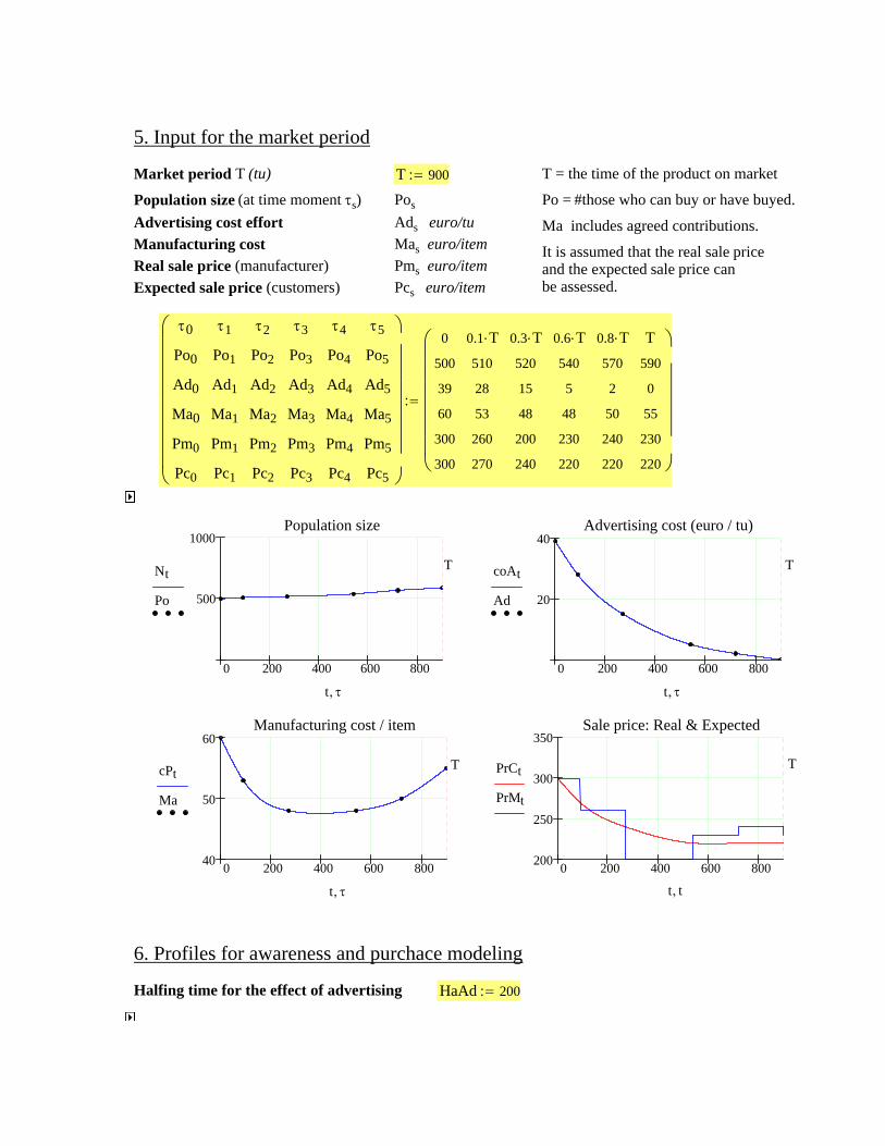
5. Input for the market period
Market period T (tu) T 900:= T = the time of the product on market Po = #those who can buy or have buyed. Ma includes agreed contributions.
It is assumed that the real sale price
and the expected sale price can be assessed.
Population size (at time moment τs) Pos Advertising cost effort Ads euro/tuManufacturing cost Mas euro/item Real sale price (manufacturer) Pms euro/itemExpected sale price (customers) Pcs euro/item
τ0
Po0
Ad0
Ma0
Pm0
Pc0
τ1
Po1
Ad1
Ma1
Pm1
Pc1
τ2
Po2
Ad2
Ma2
Pm2
Pc2
τ3
Po3
Ad3
Ma3
Pm3
Pc3
τ4
Po4
Ad4
Ma4
Pm4
Pc4
τ5
Po5
Ad5
Ma5
Pm5
Pc5
⎛⎜⎜⎜⎜⎜⎜⎜⎜⎝
⎞⎟⎟⎟⎟⎟⎟⎟⎟⎠
0
500
39
60
300
300
0.1 T⋅510
28
53
260
270
0.3 T⋅520
15
48
200
240
0.6 T⋅540
5
48
230
220
0.8 T⋅570
2
50
240
220
T590
0
55
230
220
⎛⎜⎜⎜⎜⎜⎜⎝
⎞⎟⎟⎟⎟⎟⎟⎠
:=
0 200 400 600 800
500
1000Population size
Nt
Po
T
t τ,
0 200 400 600 800
20
40Advertising cost (euro / tu)
coAt
Ad
T
t τ,
0 200 400 600 80040
50
60Manufacturing cost / item
cPt
Ma
T
t τ,
0 200 400 600 800200
250
300
350Sale price: Real & Expected
PrCt
PrMt
T
t t,
6. Profiles for awareness and purchace modeling
Halfing time for the effect of advertising HaAd 200:=
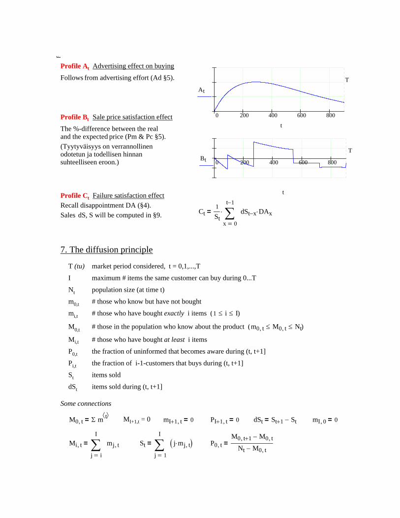
P0 t,M0 t 1+, M0 t,−
Nt M0 t,−=St
1
I
j
j mj t,⋅( )∑=
=Mi t,
i
I
j
mj t,∑=
=
mI 0, 0=dSt St 1+ St−=PI 1+ t, 0=mI 1+ t, 0=MI+1,t = 0 M0 t, Σ m t⟨ ⟩=
Some connections
T (tu) market period considered, t = 0,1,...,T
I maximum # items the same customer can buy during 0...T
Nt population size (at time t)
m0,t # those who know but have not bought mi,t # those who have bought exactly i items (1 i≤ I≤ )
M0,t # those in the population who know about the product (m0 t, M0 t,≤ Nt≤ )
Mi,t # those who have bought at least i items P0,t the fraction of uninformed that becomes aware during (t, t+1]
Pi,t the fraction of i-1-customers that buys during (t, t+1]
St items sold dSt items sold during (t, t+1]
7. The diffusion principle
Ct1St
0
t 1−
x
dSt x− DAx⋅∑=
⋅=
Profile Ct Failure satisfaction effectRecall disappointment DA (§4). Sales dS, S will be computed in §9.
0 200 400 600 800Bt
T
t
Profile Bt Sale price satisfaction effect The %-difference between the real and the expected price (Pm & Pc §5).(Tyytyväisyys on verrannollinen odotetun ja todellisen hinnan suhteelliseen eroon.)
Profile At Advertising effect on buying
Follows from advertising effort (Ad §5).
0 200 400 600 800
At
T
t
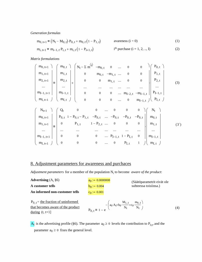
At is the advertising profile (§6). The parameter a0 0≥ levels the contribution to P0,t, and the
parameter a0 0≥ fixes the general level.
P0 t, 1 ea0 At⋅ b0
M1 t,
Nt⋅+ c0
m0 t,
Nt⋅+
⎛⎜⎝
⎞⎟⎠
−
−= (4)
P0 t, = the fraction of uninformed that becomes aware of the product during (t, t+1]
c0 0.001:=An informed non-customer tellsb0 0.004:=A customer tells
(Säätöparametrit eivät ole suhteessa toisiinsa.)
a0 0.0000008:=Advertising (At §6)
Adjustment parameters for a member of the population Nt to become aware of the product:
8. Adjustment parameters for awareness and purchaces
Nt 1+
m0 t 1+,
m1 t 1+,
....
mI 1− t 1+,
mI t 1+,
⎛⎜⎜⎜⎜⎜⎜⎜⎜⎝
⎞⎟⎟⎟⎟⎟⎟⎟⎟⎠
Qt
P0 t,
0
....
0
0
0
1 P0 t,− P1 t,−
P1 t,
....
0
0
0
P0 t,−
1 P2 t,−
....
0
0
....
....
....
....
....
....
0
P0 t,−
0
....
PI 1− t,
0
0
P0 t,−
0
....
1 PI t,−
PI t,
0
P0 t,−
0
....
0
1
⎛⎜⎜⎜⎜⎜⎜⎜⎜⎝
⎞⎟⎟⎟⎟⎟⎟⎟⎟⎠
Nt
m0 t,
m1 t,
....
mI 1− t,
mI t,
⎛⎜⎜⎜⎜⎜⎜⎜⎜⎝
⎞⎟⎟⎟⎟⎟⎟⎟⎟⎠
⋅= 3´( )
(3)
m0 t 1+,
m1 t 1+,
m2 t 1+,
....
mI 1− t 1+,
mI t 1+,
⎛⎜⎜⎜⎜⎜⎜⎜⎜⎝
⎞⎟⎟⎟⎟⎟⎟⎟⎟⎠
m0 t,
m1 t,
m2 t,
....
mI 1− t,
mI t,
⎛⎜⎜⎜⎜⎜⎜⎜⎜⎝
⎞⎟⎟⎟⎟⎟⎟⎟⎟⎠
Nt Σ m t⟨ ⟩−
0
0
....
0
0
m0 t,−
m0 t,
0
....
0
0
0
m1 t,−
m1 t,
....
0
0
....
....
....
....
....
....
0
0
0
....
mI 2− t,
0
0
0
0
....
mI 1− t,−
mI 1− t,
⎛⎜⎜⎜⎜⎜⎜⎜⎜⎝
⎞⎟⎟⎟⎟⎟⎟⎟⎟⎠
P0 t,
P1 t,
P2 t,
....
PI 1− t,
PI t,
⎛⎜⎜⎜⎜⎜⎜⎜⎜⎝
⎞⎟⎟⎟⎟⎟⎟⎟⎟⎠
⋅+=
Matrix formulations
(2)ith purchase (i = 1, 2, .., I)mi t 1+, mi 1− t, Pi t,⋅ mi t, 1 Pi 1+ t,−( )⋅+=
(1)avareness (i = 0)m0 t 1+, Nt M0 t,−( ) P0 t,⋅ m0 t, 1 P1 t,−( )⋅+=
Generation formulas
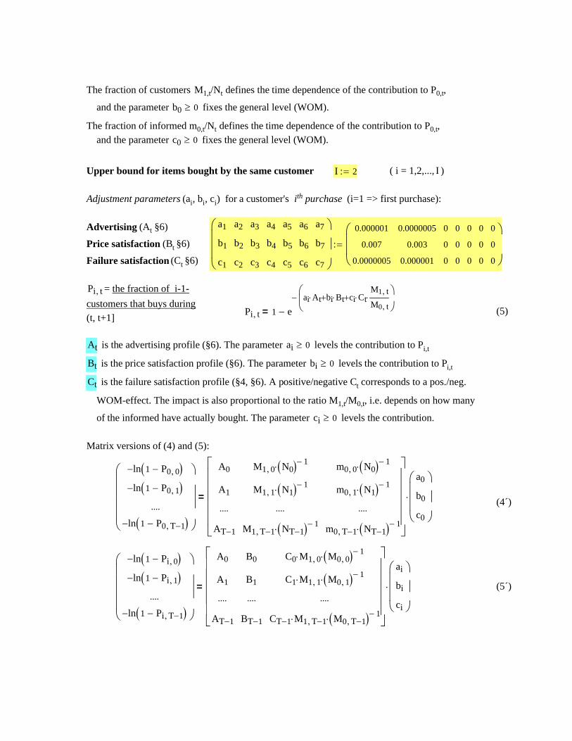
The fraction of customers M1,t/Nt defines the time dependence of the contribution to P0,t,
and the parameter b0 0≥ fixes the general level (WOM).
The fraction of informed m0,t/Nt defines the time dependence of the contribution to P0,t, and the parameter c0 0≥ fixes the general level (WOM).
Upper bound for items bought by the same customer I 2:= ( i = 1,2,..., I )
Adjustment parameters (ai, bi, ci) for a customer's ith purchase (i=1 => first purchase):
Advertising (At §6)
Price satisfaction (Bt §6)
Failure satisfaction (Ct §6)
a1
b1
c1
a2
b2
c2
a3
b3
c3
a4
b4
c4
a5
b5
c5
a6
b6
c6
a7
b7
c7
⎛⎜⎜⎜⎝
⎞⎟⎟⎟⎠
0.000001
0.007
0.0000005
0.0000005
0.003
0.000001
0
0
0
0
0
0
0
0
0
0
0
0
0
0
0
⎛⎜⎜⎝
⎞⎟⎟⎠
:=
Pi t, = the fraction of i-1-customers that buys during (t, t+1] Pi t, 1 e
ai At⋅ bi Bt⋅+ ci Ct⋅M1 t,
M0 t,⋅+
⎛⎜⎝
⎞⎟⎠
−
−= (5)
At is the advertising profile (§6). The parameter ai 0≥ levels the contribution to Pi,t
Bt is the price satisfaction profile (§6). The parameter bi 0≥ levels the contribution to Pi,t
Ct is the failure satisfaction profile (§4, §6). A positive/negative Ct corresponds to a pos./neg.
WOM-effect. The impact is also proportional to the ratio M1,t/M0,t, i.e. depends on how many
of the informed have actually bought. The parameter ci 0≥ levels the contribution.
Matrix versions of (4) and (5):
ln 1 P0 0,−( )−
ln 1 P0 1,−( )−
....
ln 1 P0 T 1−,−( )−
⎛⎜⎜⎜⎜⎝
⎞⎟⎟⎟⎟⎠
A0
A1
....
AT 1−
M1 0, N0( ) 1−⋅
M1 1, N1( ) 1−⋅
....
M1 T 1−, NT 1−( ) 1−⋅
m0 0, N0( ) 1−⋅
m0 1, N1( ) 1−⋅
....
m0 T 1−, NT 1−( ) 1−⋅
⎡⎢⎢⎢⎢⎢⎣
⎤⎥⎥⎥⎥⎥⎦
a0
b0
c0
⎛⎜⎜⎜⎝
⎞⎟⎟⎟⎠
⋅= (4´)
ln 1 Pi 0,−( )−
ln 1 Pi 1,−( )−
....
ln 1 Pi T 1−,−( )−
⎛⎜⎜⎜⎜⎝
⎞⎟⎟⎟⎟⎠
A0
A1
....
AT 1−
B0
B1
....
BT 1−
C0 M1 0,⋅ M0 0,( ) 1−⋅
C1 M1 1,⋅ M0 1,( ) 1−⋅
....
CT 1− M1 T 1−,⋅ M0 T 1−,( ) 1−⋅
⎡⎢⎢⎢⎢⎢⎣
⎤⎥⎥⎥⎥⎥⎦
ai
bi
ci
⎛⎜⎜⎜⎝
⎞⎟⎟⎟⎠
⋅= (5´)
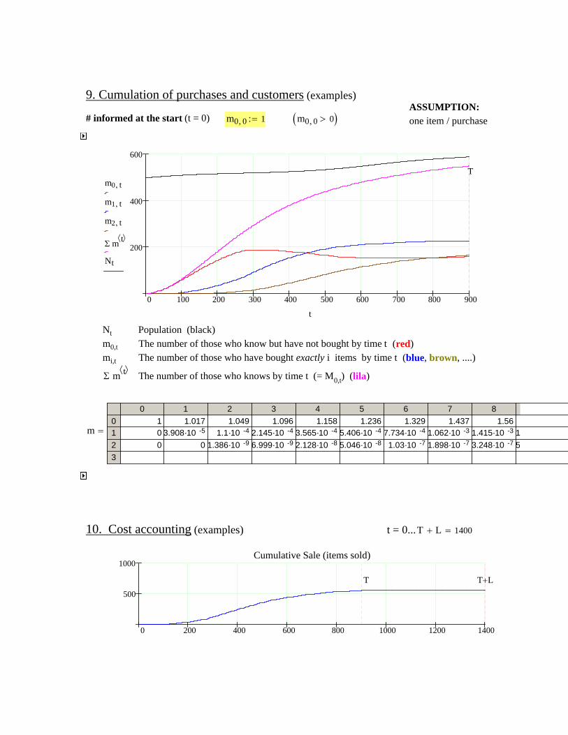
9. Cumulation of purchases and customers (examples)ASSUMPTION: one item / purchase # informed at the start (t = 0) m0 0, 1:= m0 0, 0>( )
0 100 200 300 400 500 600 700 800 900
200
400
600
m0 t,
m1 t,
m2 t,
Σ m t⟨ ⟩
Nt
T
t
Nt Population (black) m0,t The number of those who know but have not bought by time t (red) mi,t The number of those who have bought exactly i items by time t (blue, brown, ....)
Σ m t⟨ ⟩ The number of those who knows by time t (= M0,t) (lila)
m
0 1 2 3 4 5 6 7 80123
1 1.017 1.049 1.096 1.158 1.236 1.329 1.437 1.560 3.908·10 -5 1.1·10 -4 2.145·10 -4 3.565·10 -4 5.406·10 -4 7.734·10 -4 1.062·10 -3 1.415·10 -3 10 0 1.386·10 -9 6.999·10 -9 2.128·10 -8 5.046·10 -8 1.03·10 -7 1.898·10 -7 3.248·10 -7 5
=
10. Cost accounting (examples) t = 0...T L+ 1400=
0 200 400 600 800 1000 1200 1400
500
1000Cumulative Sale (items sold)
T L+T
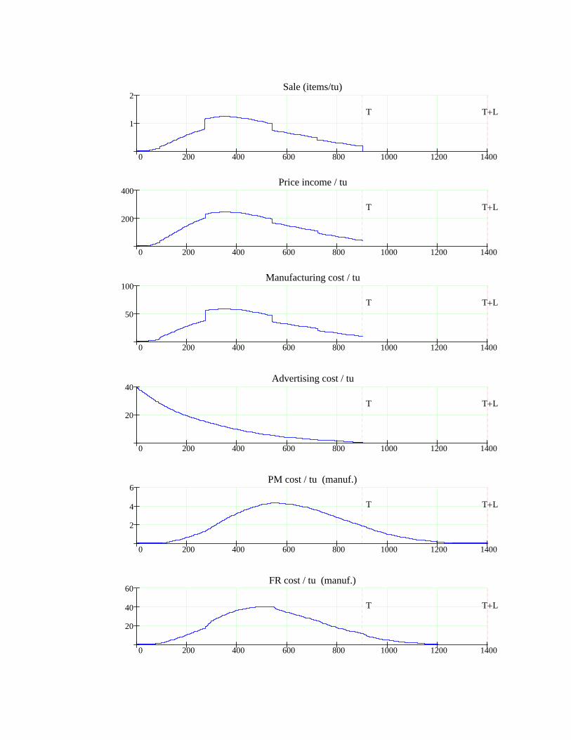
0 200 400 600 800 1000 1200 1400
1
2Sale (items/tu)
T L+T
0 200 400 600 800 1000 1200 1400
200
400Price income / tu
T L+T
0 200 400 600 800 1000 1200 1400
50
100Manufacturing cost / tu
T L+T
0 200 400 600 800 1000 1200 1400
20
40Advertising cost / tu
T L+T
0 200 400 600 800 1000 1200 1400
2
4
6PM cost / tu (manuf.)
T L+T
0 200 400 600 800 1000 1200 1400
20
40
60FR cost / tu (manuf.)
T L+T
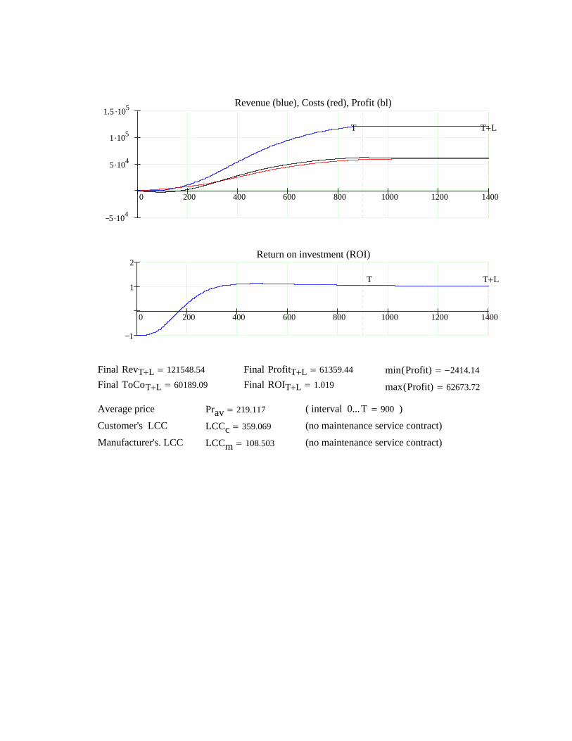
0 200 400 600 800 1000 1200 1400
5 .104
5 .104
1 .105
1.5 .105 Revenue (blue), Costs (red), Profit (bl)
T T L+
0 200 400 600 800 1000 1200 1400
1
1
2Return on investment (ROI)
T L+T
Final RevT L+ 121548.54= Final ToCoT L+ 60189.09=
Final ProfitT L+ 61359.44=Final ROIT L+ 1.019=
min Profit( ) 2414.14−=
max Profit( ) 62673.72=
Average price Prav 219.117= ( interval 0...T 900= )
Customer's LCC LCCc 359.069= (no maintenance service contract)
Manufacturer's. LCC LCCm 108.503= (no maintenance service contract)

Diffusion Model II Comments: [email protected]
Tämä on yhden tuotteen metamalli, jossa suureiden muuttuminen lasketaan diffuusioperiaatteella sekä tuoteyksilön elinaikana että markkinajakson aikana. Malli muistuttaa edellistä (Diffusion Model I), mutta on tarkempi ja laajempi.
Määritellään edelleen eri vikatyyppien esiintymistä ja niiden aiheuttamat kustannukset (FR), ennakko- huollon kustannukset (PM), takuusopimus ja huoltosopimus, populaatio, satsaus mainostamiseen, todellinen ja odotettu myyntihinta, asiakastyytyväisyys liittyen hintaan ja vikoihin, ym. sekä näiden mahdollinen aikariippuvuus. Perusmalleja on paikoittain kehitetty syötön ja/tai matemaattisen käsittelyn osalta oleellisesti.
Kokonaan uusia elementtejä ovat esimerkiksi uudelleenoston ja asiakkuudesta luopumisen tarkka mallinnus, asiakkaan oman kokemuksen ja kilpailevien valmistajien vaikutus myyntiin, sekä epäkäytettävyyden vaikutus tyytyväisyyteen.
Rakennetaan ostojen ajasta riippuvat "todennäköisyydet" ottaen myös humioon kuinka mones osto on kyseessä. Säätöparametrit ja rinnakkaiset differenssiyhtälöt ohjaavat markkinatilan ajallista muuttumista, eli erilaisten asiakaslukumäärien kehittymistä (potentiaaliset ostajat, kerran ostaneet, kaksikertaa ostaneet, jne.).
Lopuksi kustannuslaskentaa. Diffuusion tuottamasta perusdatasta malli laskee kustannusten, tulojen, profiittien ym. ajallista kehittymistä markkinajaksolla.
Syötöt keltaisella!
1. Product's failure tendency (item)
Essential lifetime of an item (tu) L 220:= The average number vc,f of f-failures during the interval 0...xc.
f=1
f=2
f=3
Failure types: f = 1,2,3Vikatyypit ovat täysinvapaasti määriteltävissä.
x1
v1 1,
v1 2,
v1 3,
x2
v2 1,
v2 2,
v2 3,
x3
v3 1,
v3 2,
v3 3,
x4
v4 1,
v4 2,
v4 3,
x5
v5 1,
v5 2,
v5 3,
⎛⎜⎜⎜⎜⎝
⎞⎟⎟⎟⎟⎠
0.05 L⋅0.5
0.1
0.1
0.2 L⋅0.7
0.2
0.2
0.4 L⋅0.8
0.4
0.4
0.7 L⋅1
1.4
1
L1.4
3.4
2.4
⎛⎜⎜⎜⎝
⎞⎟⎟⎟⎠
:=

f=0 f=1 f=2 f=3
Fraction at L
Fraction at W+
Costs in W...L
Fraction at W
Fraction at V+
C10
V0
pV0
qV0
C20
W0
pW0
qW0
C30
pL0
qL0
C11
V1
pV1
qV1
C21
W1
pW1
qW1
C31
pL1
qL1
C12
V2
pV2
qV2
C22
W2
pW2
qW2
C32
pL2
qL2
C13
V3
pV3
qV3
C23
W3
pW3
qW3
C33
pL3
qL3
⎛⎜⎜⎜⎜⎜⎜⎜⎜⎜⎜⎜⎜⎜⎜⎜⎝
⎞⎟⎟⎟⎟⎟⎟⎟⎟⎟⎟⎟⎟⎟⎟⎟⎠
0.18
0.3 L⋅0.3
0.2
0.18
0.6 L⋅0.2
0.1
0.15
0
0
50
0.3 L⋅0.8
0.8
40
0.6 L⋅0.8
0.5
50
0
0
50
0.4 L⋅0.8
0.8
40
0.6 L⋅0.6
0.2
50
0
0
50
0.4 L⋅0.8
0.8
40
0.7 L⋅0.6
0.2
50
0
0
⎛⎜⎜⎜⎜⎜⎜⎜⎜⎜⎜⎜⎜⎜⎝
⎞⎟⎟⎟⎟⎟⎟⎟⎟⎟⎟⎟⎟⎟⎠
:= End point W
Costs in V...W
Fraction at V
Fraction at 0+
End point V
Costs in 0...V
Every product support cost (to be considered) must be placed in one of the following four classes:
Preventive maintenance (PM) costs C0 euro /tu (f = 0)
Failure related (FR) costs Cf euro /f-failure (f = 1,2,3, §1)
for subintervals (α, β] = (0,Vf ], (Vf,Wf] and (Wf ,L], respectively. In each subinterval, manufacturer's warranty fraction varies from pf to qf:
Cf pf qf pf−( ) x α−
β α−⎛⎜⎝
⎞⎟⎠
⋅+⎡⎢⎣
⎤⎥⎦
⋅ x∈ (α, β] f = 0, 1, 2, 3.
2. Costs and the warranty contract (item)
Failure tendencies Λx,f
i.e. # f-failures /item 0...x
(f = 1, 2, 3)
0 50 100 150 200
2
4# f-failures in 0...x
Λx 1,
Λx 2,
Λx 3,
L
x

Examples pV qV= 1= FRW-warranty on 0...V with manufacturer's full responsibility
pV qV 1<= FRW-warranty on 0...V with manufacturer's partial responsibility pW qW≠ PRW-warranty on V ..W, manufacturer's time dependent responsibility
3. Cumulative costs and maintenance service contract (item)
Cumulative PM and FR costs /item during 0...L
(manufacturer's cost = solid, customer's cost = dot, total = dash)
0 100 200
20
40PM cost f=0
V0 W0
0 100 200
50
100FR cost f=1
W1V1
0 100 200
100
200FR cost f=2
W2V2
0 100 200
50
100
150FR cost f=3
W3V3
The customer pays FR costs during warranty periods 0...Wf : FaiReal 49.321= (totally).
Maintenance Service Contract. The costs not covered by warranty (dot curves above) can be managed by a separately bought. The customer pays MSc /tu from xc tu .
x0
MS0
x1
MS1
x2
MS2
x3
MS3
x4
MS4
⎛⎜⎝
⎞⎟⎠
0
0.5
0.3 L⋅0.7
0.4 L⋅1.0
0.6 L⋅1.2
0.8 L⋅1.8
⎛⎜⎝
⎞⎟⎠
:=
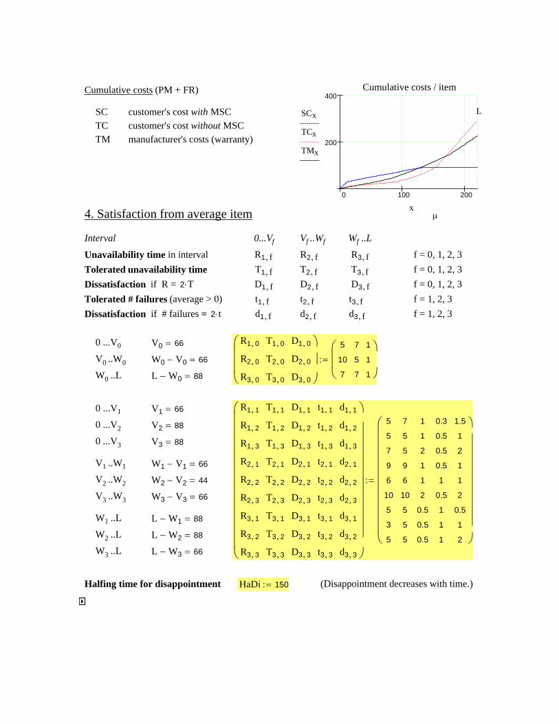
(Disappointment decreases with time.)HaDi 150:=Halfing time for disappointment
L W3− 66=
L W2− 88=
L W1− 88=W1 ..L
W2 ..L
W3 ..L
W3 V3− 66=
R1 1,
R1 2,
R1 3,
R2 1,
R2 2,
R2 3,
R3 1,
R3 2,
R3 3,
T1 1,
T1 2,
T1 3,
T2 1,
T2 2,
T2 3,
T3 1,
T3 2,
T3 3,
D1 1,
D1 2,
D1 3,
D2 1,
D2 2,
D2 3,
D3 1,
D3 2,
D3 3,
t1 1,
t1 2,
t1 3,
t2 1,
t2 2,
t2 3,
t3 1,
t3 2,
t3 3,
d1 1,
d1 2,
d1 3,
d2 1,
d2 2,
d2 3,
d3 1,
d3 2,
d3 3,
⎛⎜⎜⎜⎜⎜⎜⎜⎜⎜⎜⎜⎜⎝
⎞⎟⎟⎟⎟⎟⎟⎟⎟⎟⎟⎟⎟⎠
5
5
7
9
6
10
5
3
5
7
5
5
9
6
10
5
5
5
1
1
2
1
1
2
0.5
0.5
0.5
0.3
0.5
0.5
0.5
1
0.5
1
1
1
1.5
1
2
1
1
2
0.5
1
2
⎛⎜⎜⎜⎜⎜⎜⎜⎜⎜⎜⎝
⎞⎟⎟⎟⎟⎟⎟⎟⎟⎟⎟⎠
:=W2 V2− 44=
W1 V1− 66=V1 ..W1
V2 ..W2
V3 ..W3
V3 88=
V2 88=
V1 66=0 ...V1
0 ...V2
0 ...V3
L W0− 88=
R1 0,
R2 0,
R3 0,
T1 0,
T2 0,
T3 0,
D1 0,
D2 0,
D3 0,
⎛⎜⎜⎜⎝
⎞⎟⎟⎟⎠
5
10
7
7
5
7
1
1
1
⎛⎜⎜⎝
⎞⎟⎟⎠
:=W0 V0− 66=
V0 66=0 ...V0
V0 ..W0
W0 ..L
Unavailability time in interval R1 f, R2 f, R3 f, f = 0, 1, 2, 3Tolerated unavailability time T1 f, T2 f, T3 f, f = 0, 1, 2, 3Dissatisfaction if R = 2 T⋅ D1 f, D2 f, D3 f, f = 0, 1, 2, 3Tolerated # failures (average > 0) t1 f, t2 f, t3 f, f = 1, 2, 3Dissatisfaction if # failures = 2 t⋅ d1 f, d2 f, d3 f, f = 1, 2, 3
0...Vf Vf ..Wf Wf ..LInterval
4. Satisfaction from average item
SC customer's cost with MSC TC customer's cost without MSC TM manufacturer's costs (warranty)
Cumulative costs (PM + FR)
0 100 200
200
400Cumulative costs / item
SCx
TCx
TMx
L
μx

0 100 200 300 400
1
1
2
# failuresunavailabilitytotal
Satisfaction during & after item's life
FaSax
SeSax
Satisx
L
x
5. Repeat purchases and lost customers
i-customer = potential or non-lost customer that has bought exactly i times ( i 0≥ ).
Decision. Let X (tu) denote the age of a bought item when the customer in question makes the following decision: He/she
EITHER (a) buys for the ith time (i.e. becomes an i-customer) OR (b) gives up the customership (i.e. becomes a lost i-1-customer)
Average for X (tu) μ 200:=
Deviation for X (tu) σ 25:= (σ < μ)
0 50 100 150 200 250 300 350 400
0.01
0.02Density for X
dFxμ L
x
Average satisfaction (§4) at the moment of decision
Own
x
Satisx dFx⋅∑:= Own 0.8=
Fractions for alternatives (a) or (b) (will be defined in §8). If an i-1-customer bought his/her
i-1th item during ( t 1− , t], then he/she will make the decision during (t X+ 1− , t X+ ]. The corresponding "probabilities" (fractions) are Pi t X+ 1−, for (a), and 1 Pi t X+ 1−,− for (b).
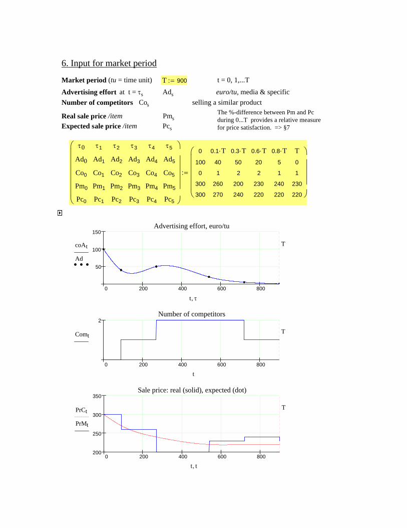
6. Input for market period
Market period (tu = time unit) T 900:= t = 0, 1,...T
Advertising effort at t = τs Ads euro/tu, media & specificNumber of competitors Cos selling a similar product
The %-difference between Pm and Pc during 0...T provides a relative measure for price satisfaction. => §7
Real sale price /item PmsExpected sale price /item Pcs
τ0
Ad0
Co0
Pm0
Pc0
τ1
Ad1
Co1
Pm1
Pc1
τ2
Ad2
Co2
Pm2
Pc2
τ3
Ad3
Co3
Pm3
Pc3
τ4
Ad4
Co4
Pm4
Pc4
τ5
Ad5
Co5
Pm5
Pc5
⎛⎜⎜⎜⎜⎜⎜⎝
⎞⎟⎟⎟⎟⎟⎟⎠
0
100
0
300
300
0.1 T⋅40
1
260
270
0.3 T⋅50
2
200
240
0.6 T⋅20
2
230
220
0.8 T⋅5
1
240
220
T0
1
230
220
⎛⎜⎜⎜⎜⎜⎝
⎞⎟⎟⎟⎟⎟⎠
:=
0 200 400 600 800
50
100
150Advertising effort, euro/tu
coAt
Ad
T
t τ,
0 200 400 600 800
2Number of competitors
ComtT
t
0 200 400 600 800200
250
300
350Sale price: real (solid), expected (dot)
PrCt
PrMt
T
t t,

α1
β1
γ1
δ1
ε1
α2
β2
γ2
δ2
ε2
α3
β3
γ3
δ3
ε3
α4
β4
γ4
δ4
ε4
α5
β5
γ5
δ5
ε5
α6
β6
γ6
δ6
ε6
⎛⎜⎜⎜⎜⎜⎜⎝
⎞⎟⎟⎟⎟⎟⎟⎠
0.4 10 5−⋅0.05
0.2
0.5
0
0.4 10 5−⋅0.05
0.2
0.5
0.5
0.4 10 5−⋅0.05
0.2
0.5
1
0
0.05
0.2
0.5
1.5
0
0.05
0.2
0.2
2
0
0.05
0.2
0
2
⎛⎜⎜⎜⎜⎜⎝
⎞⎟⎟⎟⎟⎟⎠
:=
Advertising
Competitors effect
Sale price satisfaction
WOM (fail. & unavail.)
Own experience
Adjustment parameters αi βi, γi, δi, εi,( ) for a customer's ith purchase (i 1= 2, 3, 4, 5, 6, )
8. Purchase fractions and the structure of diffusion
SatProt1
Qt 1−1
t 1−
s
dQs Satist s−⋅∑=
⋅=Satis was defined in §4. SatPro will be computed in §9. (Qt = #purchases 0...t, §5)
General satisfaction with failures andunavailability at t
Satisfaction with purchase price. (From Pm & Pc §6.)
0 200 400 600 800
0.2
0.1
0.1
0.2
SatPritT
t
Impact of competitors. (From Co, §6.)
0 200 400 600 800
1
2
ImCotT
t
Impact of advertising. (From Ad, §6.)
0 200 400 600 800
5000
1 .1041.5 .104
2 .104
Vist
T
t
HaAd 400:=Halfing time for effect of advertising effort:
7. Profiles for market period
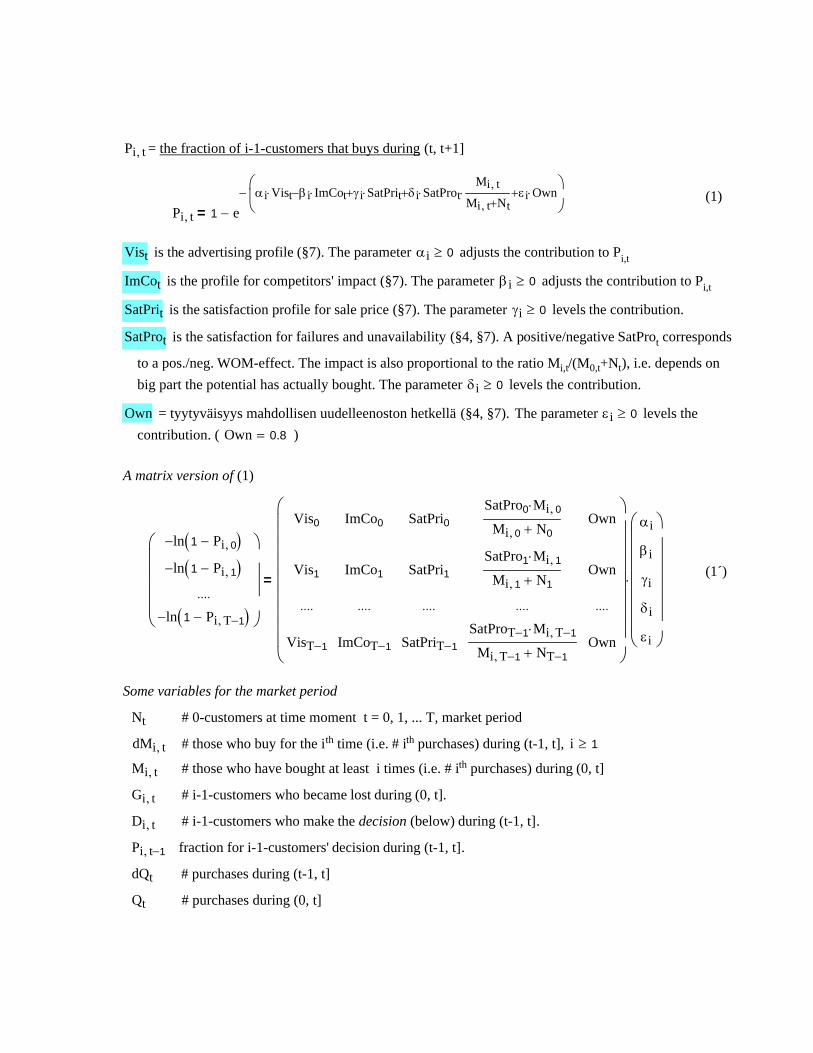
Pi t, = the fraction of i-1-customers that buys during (t, t+1]
(1)Pi t, 1 e
αi Vist⋅ βi ImCot⋅− γ i SatPrit⋅+ δi SatProt⋅Mi t,
Mi t, Nt+⋅+ εi Own⋅+
⎛⎜⎝
⎞⎟⎠
−
−=
Vist is the advertising profile (§7). The parameter αi 0≥ adjusts the contribution to Pi,t
ImCot is the profile for competitors' impact (§7). The parameter βi 0≥ adjusts the contribution to Pi,t
SatPrit is the satisfaction profile for sale price (§7). The parameter γi 0≥ levels the contribution.
SatProt is the satisfaction for failures and unavailability (§4, §7). A positive/negative SatProt corresponds
to a pos./neg. WOM-effect. The impact is also proportional to the ratio Mi,t/(M0,t+Nt), i.e. depends on big part the potential has actually bought. The parameter δi 0≥ levels the contribution.
Own = tyytyväisyys mahdollisen uudelleenoston hetkellä (§4, §7). The parameter εi 0≥ levels the contribution. ( Own 0.8= )
A matrix version of (1)
(1´)
ln 1 Pi 0,−( )−
ln 1 Pi 1,−( )−
....
ln 1 Pi T 1−,−( )−
⎛⎜⎜⎜⎜⎝
⎞⎟⎟⎟⎟⎠
Vis0
Vis1
....
VisT 1−
ImCo0
ImCo1
....
ImCoT 1−
SatPri0
SatPri1
....
SatPriT 1−
SatPro0 Mi 0,⋅
Mi 0, N0+
SatPro1 Mi 1,⋅
Mi 1, N1+
....
SatProT 1− Mi T 1−,⋅
Mi T 1−, NT 1−+
Own
Own
....
Own
⎛⎜⎜⎜⎜⎜⎜⎜⎜⎜⎝
⎞⎟⎟⎟⎟⎟⎟⎟⎟⎟⎠
αi
βi
γi
δi
εi
⎛⎜⎜⎜⎜⎜⎜⎜⎝
⎞⎟⎟⎟⎟⎟⎟⎟⎠
⋅=
Some variables for the market period
Nt # 0-customers at time moment t = 0, 1, ... T, market period
dMi t, # those who buy for the ith time (i.e. # ith purchases) during (t-1, t], i 1≥
Mi t, # those who have bought at least i times (i.e. # ith purchases) during (0, t]
Gi t, # i-1-customers who became lost during (0, t].
Di t, # i-1-customers who make the decision (below) during (t-1, t].
Pi t 1−, fraction for i-1-customers' decision during (t-1, t].
dQt # purchases during (t-1, t]
Qt # purchases during (0, t]
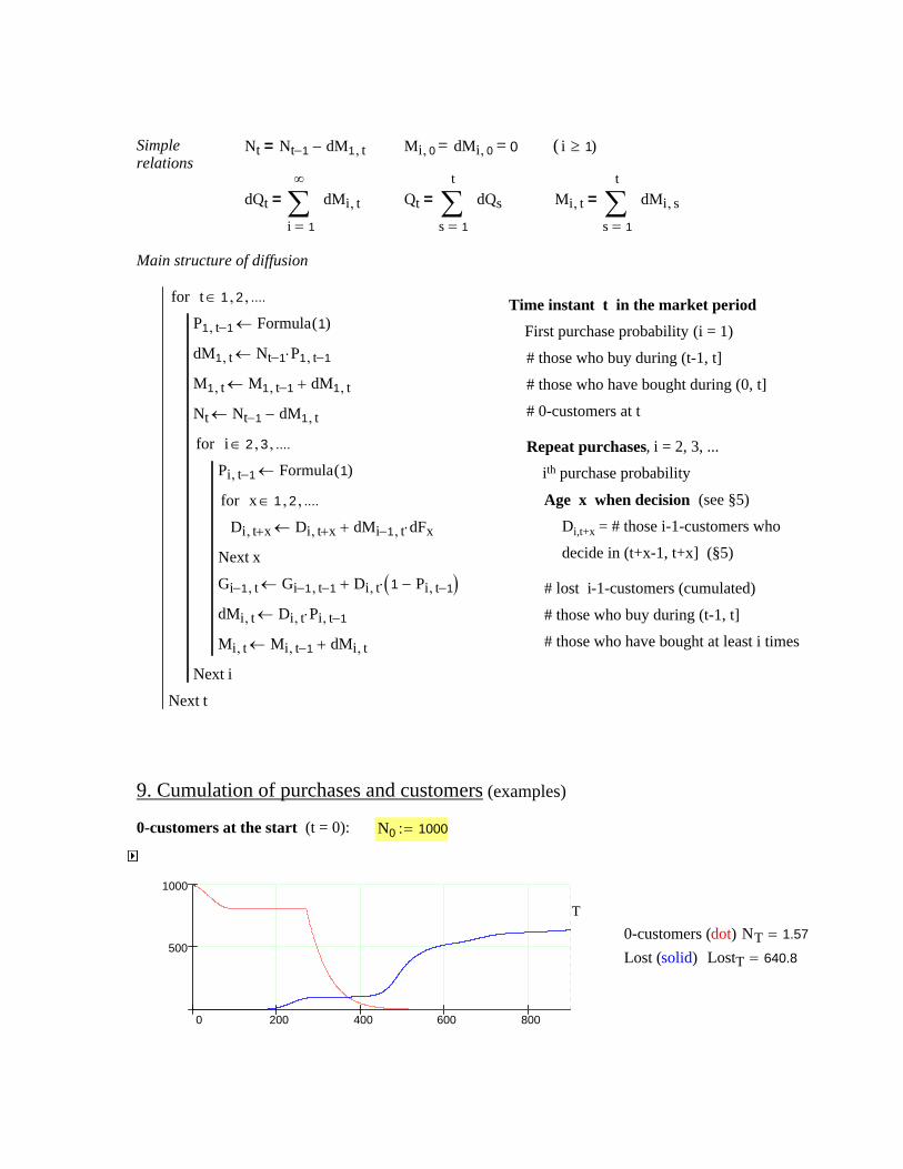
0-customers (dot) NT 1.57=Lost (solid) LostT 640.8=
0 200 400 600 800
500
1000
T
N0 1000:=0-customers at the start (t = 0):
9. Cumulation of purchases and customers (examples)
# those who have bought at least i times
# those who buy during (t-1, t]
# lost i-1-customers (cumulated)
Di,t+x = # those i-1-customers who
decide in (t+x-1, t+x] (§5)
Age x when decision (see §5)
Repeat purchases, i = 2, 3, ... ith purchase probability
# 0-customers at t
# those who have bought during (0, t]
# those who buy during (t-1, t]
Time instant t in the market period
First purchase probability (i = 1) P1 t 1−, Formula 1( )←
dM1 t, Nt 1− P1 t 1−,⋅←
M1 t, M1 t 1−, dM1 t,+←
Nt Nt 1− dM1 t,−←
Pi t 1−, Formula 1( )←
Di t x+, Di t x+, dMi 1− t, dFx⋅+←
x 1 2, ....,∈for
Next x
Gi 1− t, Gi 1− t 1−, Di t, 1 Pi t 1−,−( )⋅+←
dMi t, Di t, Pi t 1−,⋅←
Mi t, Mi t 1−, dMi t,+←
i 2 3, ....,∈for
Next i
t 1 2, ....,∈for
Next t
Main structure of diffusion
Mi t,
1
t
s
dMi s,∑=
=Qt1
t
s
dQs∑=
=dQt1
∞
i
dMi t,∑=
=
( i 1≥ ) Mi 0, = dMi 0, = 0Nt Nt 1− dM1 t,−=Simplerelations
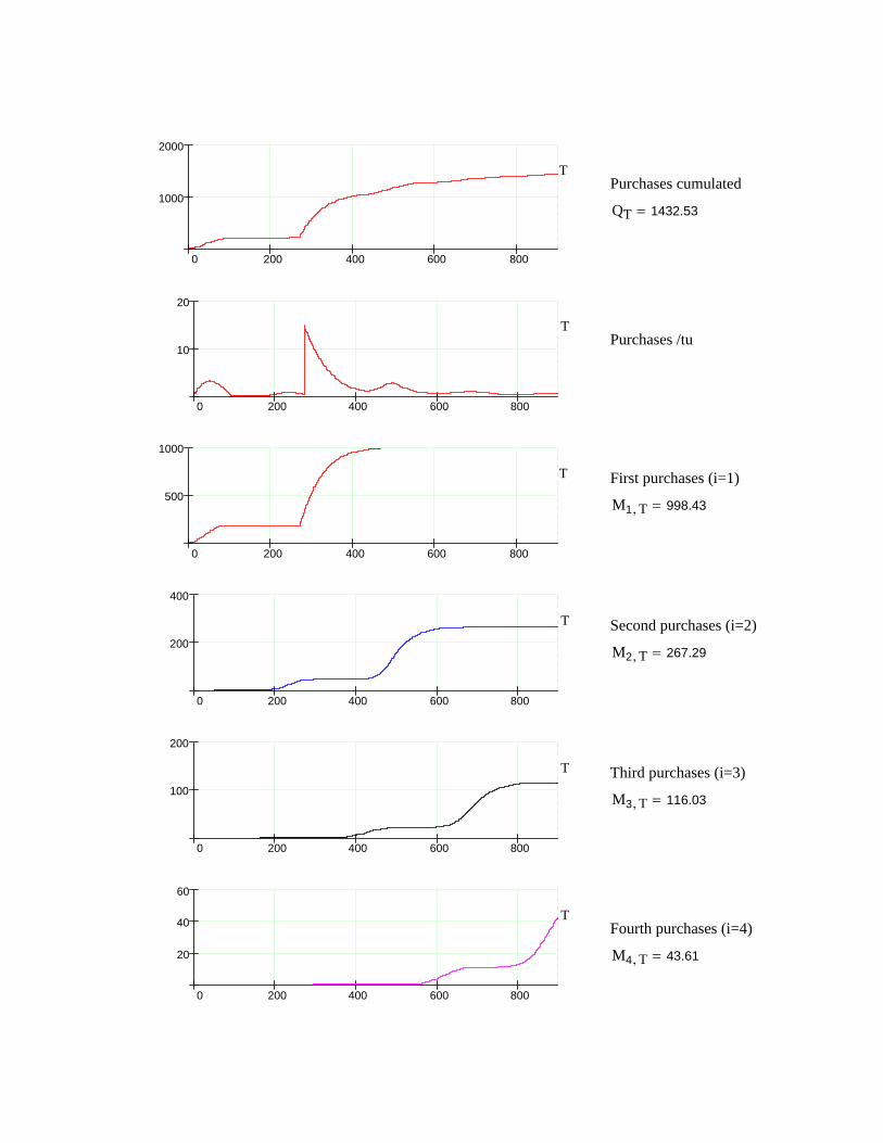
M4 T, 43.61=
Fourth purchases (i=4)
0 200 400 600 800
20
40
60
T
M3 T, 116.03=
Third purchases (i=3)
0 200 400 600 800
100
200
T
M2 T, 267.29=
Second purchases (i=2)
0 200 400 600 800
200
400
T
M1 T, 998.43=
First purchases (i=1)
0 200 400 600 800
500
1000
T
Purchases /tu
0 200 400 600 800
10
20
T
QT 1432.53=
Purchases cumulated
0 200 400 600 800
1000
2000
T
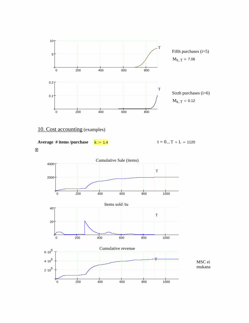
0 200 400 600 800
5
10
TFifth purchases (i=5)
M5 T, 7.06=
0 200 400 600 800
0.1
0.2
TSixth purchases (i=6)
M6 T, 0.12=
10. Cost accounting (examples)
Average # items /purchase k 1.4:= t = 0...T L+ 1120=
0 200 400 600 800 1000
2000
4000Cumulative Sale (items)
T
0 200 400 600 800 1000
20
40Items sold /tu
T
0 200 400 600 800 1000
2 .105
4 .105
6 .105 Cumulative revenue
TMSC eimukana
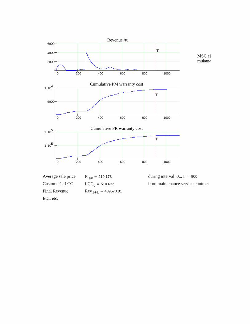
0 200 400 600 800 1000
2000
4000
6000Revenue /tu
TMSC eimukana
0 200 400 600 800 1000
5000
1 .104 Cumulative PM warranty cost
T
0 200 400 600 800 1000
1 .105
2 .105 Cumulative FR warranty cost
T
Average sale price Prav 219.178= during interval 0...T 900=
Customer's LCC LCCc 510.632= if no maintenance service contract
Final Revenue RevT L+ 439570.81=
Etc., etc.

SOME OUTPUTS
LostT 0 1 2 3 4 5 60 0 0 0 0 0 0 0
=
NT 0 1 2 3 4 5 6 7 8 9 10 110 1·10 3 999.4 998.7 997.9 996.8 995.7 994.4 993 991.5 989.9 988.1 986.3
=
G
893 894 895 896 897 898 899 9000123456
0 0 0 0 0 0 0 0523.219 523.219 523.219 523.219 523.219 523.219 523.219 523.21995.217 95.225 95.232 95.239 95.246 95.253 95.26 95.26619.077 19.265 19.451 19.636 19.819 20 20.179 20.3551.895 1.897 1.898 1.9 1.902 1.904 1.905 1.9070.023 0.024 0.025 0.026 0.027 0.029 0.03 0.031
0 0 0 0 0 0 0 0
=
M
283 284 285 286 287 2880123456
0 0 0 0 0 0371.030327 382.774834 394.340486 405.723317 416.922948 427.95476846.308929 46.454668 46.589875 46.7149 46.8301 46.935867
0.00086 0.000971 0.001094 0.001232 0.001385 0.00155701.065575·10 -15 1.355909·10 -15 1.723129·10 -15 2.187011·10 -15 2.772271·10 -15
0 0 0 0 0 00 0 0 0 0 0
=
dM
284 285 286 287 288 289 290 2910123456
0 0 0 0 0 0 0 011.745 11.566 11.383 11.2 11.032 10.851 10.682 10.510.146 0.135 0.125 0.115 0.106 0.097 0.088 0.08
1.103·10 -4 1.233·10 -4 1.378·10 -4 1.538·10 -4 1.714·10 -4 1.91·10 -4 2.125·10 -4 2.363·10 -4
0 0 0 0 0 0 0 1.167·10 -15
0 0 0 0 0 0 0 00 0 0 0 0 0 0 0
=
P
0 1 2 3 4 5 6 7 80123456
0 0 0 0 0 0 0 0 00 5.691·10 -4 7.16·10 -4 8.657·10 -4 1.007·10 -3 1.149·10 -3 1.283·10 -3 1.413·10 -3 1.533·10 -3
0 0.33 0.33 0.33 0.33 0.331 0.331 0.331 0.3310 0.551 0.551 0.551 0.551 0.551 0.551 0.551 0.5520 0.699 0.699 0.699 0.699 0.699 0.699 0.698 0.6980 0.798 0.798 0.798 0.798 0.798 0.798 0.798 0.7980 0.798 0.798 0.798 0.798 0.798 0.798 0.798 0.798
=
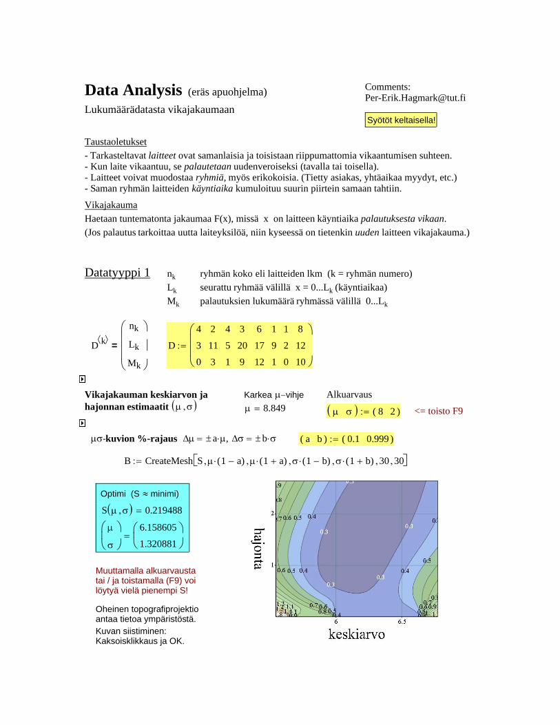
Oheinen topografiprojektioantaa tietoa ympäristöstä. Kuvan siistiminen: Kaksoisklikkaus ja OK.
Muuttamalla alkuarvaustatai / ja toistamalla (F9) voi löytyä vielä pienempi S!
Optimi (S ≈ minimi)
S μ σ,( ) 0.219488=
μ
σ
⎛⎜⎝
⎞⎟⎠
6.158605
1.320881⎛⎜⎝
⎞⎟⎠
=
B CreateMesh S μ 1 a−( )⋅, μ 1 a+( )⋅, σ 1 b−( )⋅, σ 1 b+( )⋅, 30, 30,⎡⎣ ⎤⎦:=
a b( ) 0.1 0.999( ):=μσ-kuvion %-rajaus Δμ = ±a μ⋅ , Δσ = ±b σ⋅
<= toisto F9μ σ( ) 8 2( ):=
Alkuarvaus Karkea μ−vihjeμ 8.849=
Vikajakauman keskiarvon ja hajonnan estimaatit μ σ,( )
D
4
3
0
2
11
3
4
5
1
3
20
9
6
17
12
1
9
1
1
2
0
8
12
10
⎛⎜⎜⎝
⎞⎟⎟⎠
:=D k⟨ ⟩nk
Lk
Mk
⎛⎜⎜⎜⎝
⎞⎟⎟⎟⎠
=
nk ryhmän koko eli laitteiden lkm (k = ryhmän numero)Lk seurattu ryhmää välillä x = 0...Lk (käyntiaikaa)Mk palautuksien lukumäärä ryhmässä välillä 0...Lk
Datatyyppi 1
Taustaoletukset - Tarkasteltavat laitteet ovat samanlaisia ja toisistaan riippumattomia vikaantumisen suhteen. - Kun laite vikaantuu, se palautetaan uudenveroiseksi (tavalla tai toisella). - Laitteet voivat muodostaa ryhmiä, myös erikokoisia. (Tietty asiakas, yhtäaikaa myydyt, etc.) - Saman ryhmän laitteiden käyntiaika kumuloituu suurin piirtein samaan tahtiin. Vikajakauma
Haetaan tuntematonta jakaumaa F(x), missä x on laitteen käyntiaika palautuksesta vikaan. (Jos palautus tarkoittaa uutta laiteyksilöä, niin kyseessä on tietenkin uuden laitteen vikajakauma.)
Syötöt keltaisella!
Data Analysis (eräs apuohjelma) Lukumäärädatasta vikajakaumaan
Comments: [email protected]
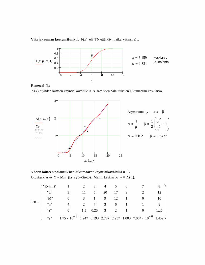
Vikajakauman kertymäfunktio F(x) eli TN että käyntiaika vikaan x≤
0 2 4 6 8 10 12
0.20.40.60.8
1
F x μ, σ, 1,( )μ
x
μ 6.159= keskiarvo ja -hajonta σ 1.321=
Renewal-fkt Λ x( ) = yhden laitteen käyntiaikavälille 0...x sattuvien palautuksien lukumäärän keskiarvo.
0 5 10 15 20 25
1
2
3
Λ x μ, σ,( )Yk
α x⋅ β+
x Lk, x,
Asymptootti y α x⋅ β+=
α1μ
= β12
σ2
μ2
1−⎛⎜⎜⎝
⎞⎟⎟⎠
⋅=
α 0.162= β 0.477−=
Yhden laitteen palautuksien lukumäärät käyntiaikaväleillä 0...L
Otoskeskiarvo Y = M/n (ks. syöttötieto). Mallin keskiarvo y Λ L( )= .
RR
"Ryhmä"
"L"
"M"
"n"
"Y"
"y"
1
3
0
4
0
1.75 10 3−×
2
11
3
2
1.5
1.247
3
5
1
4
0.25
0.193
4
20
9
3
3
2.787
5
17
12
6
2
2.257
6
9
1
1
1
1.003
7
2
0
1
0
7.004 10 6−×
8
12
10
8
1.25
1.452
⎛⎜⎜⎜⎜⎜⎜⎜⎝
⎞⎟⎟⎟⎟⎟⎟⎟⎠
=

σ 8.379=
keskiarvo ja -hajonta
μ 9.733=
0 10 20 30 40 50
0.20.40.60.8
1
F x 1, μ, σ,( )μ
x
Vikajakauman kertymäfunktio F(x) eli TN että käyntiaika vikaan x≤
Muuttamalla alkuarvaustatai / ja toistamalla (F9) voi löytyä vielä pienempi S!
Oheinen topografiprojektioantaa tietoa ympäristöstä.Kuvan siistiminen: Kaksoisklikkaus ja OK.
Optimi (S ≈ minimi)
S μ σ,( ) 0.192046=
μ
σ
⎛⎜⎝
⎞⎟⎠
9.732727
8.379457⎛⎜⎝
⎞⎟⎠
=
B CreateMesh S μ 1 a−( )⋅, μ 1 a+( )⋅, σ 1 b−( )⋅, σ 1 b+( )⋅, 30, 30,⎡⎣ ⎤⎦:=
a b( ) 0.05 0.15( ):=μσ-kuvion %-rajaus Δμ = ±a μ⋅ , Δσ = ±b σ⋅
<= toisto F9μ σ( ) 10 5( ):=
Alkuarvaus Karkea μ−vihjeμ 10.863=
Vikajakauman keskiarvon ja hajonnan estimaatit μ σ,( )
D
4
0
3
0
1
3
13
1
4
1
5
1
3
4
20
5
6
3
17
7
8
0
12
10
1
0
9
1
1
0
2
0
⎛⎜⎜⎜⎜⎝
⎞⎟⎟⎟⎟⎠
:=D k⟨ ⟩
nk
Ak
Lk
Mk
⎛⎜⎜⎜⎜⎜⎝
⎞⎟⎟⎟⎟⎟⎠
=
nk ryhmän koko eli laitteiden lkm (k = ryhmän numero)
Ak, Lk seurattu ryhmää välillä x = Ak...Lk (käyntiaikaa)Mk palautuksien lukumäärä ryhmässä välillä Ak...Lk
Datatyyppi 2

Renewal-fkt Λ x( ) = yhden laitteen käyntiaikavälille 0...x sattuvien palautuksien lukumäärän keskiarvo.
0 10 20 30 40 50
2
4
6
Λ x μ, σ,( )α x⋅ β+
x x,
Asymptootti y α x⋅ β+=
α1μ
= β12
σ2
μ2
1−⎛⎜⎜⎝
⎞⎟⎟⎠
⋅=
α 0.103= β 0.129−=
Yhden laitteen palautuksien lukumäärät käyntiaikaväleillä A...L
Otoskeskiarvo Y = M/n (ks. syöttötieto). Mallin keskiarvo y Λ L( ) Λ A( )−= .
RR
"Ryhmä"
"A"
"L"
"M"
"n"
"Y"
"y"
"Y - y"
1
0
3
0
4
0
0.219
0.219−
2
3
13
1
1
1
0.99
0.01
3
1
5
1
4
0.25
0.352
0.102−
4
4
20
5
3
1.667
1.615
0.052
5
3
17
7
6
1.167
1.399
0.233−
6
0
12
10
8
1.25
1.107
0.143
7
0
9
1
1
1
0.803
0.197
8
0
2
0
1
0
0.132
0.132−
⎛⎜⎜⎜⎜⎜⎜⎜⎜⎜⎜⎝
⎞⎟⎟⎟⎟⎟⎟⎟⎟⎟⎟⎠
=
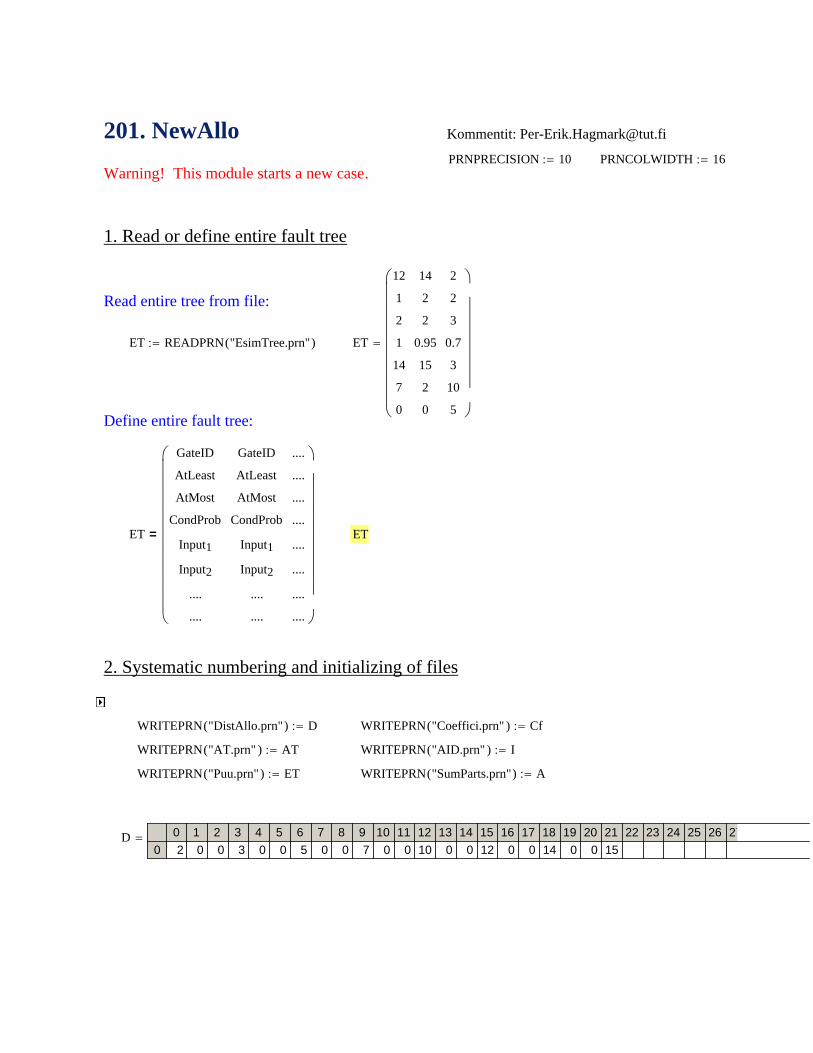
D 0 1 2 3 4 5 6 7 8 9 10 11 12 13 14 15 16 17 18 19 20 21 22 23 24 25 26 270 2 0 0 3 0 0 5 0 0 7 0 0 10 0 0 12 0 0 14 0 0 15
=
WRITEPRN "SumParts.prn"( ) A:=WRITEPRN "Puu.prn"( ) ET:=
WRITEPRN "AID.prn"( ) I:=WRITEPRN "AT.prn"( ) AT:=
WRITEPRN "Coeffici.prn"( ) Cf:=WRITEPRN "DistAllo.prn"( ) D:=
2. Systematic numbering and initializing of files
ETET
GateID
AtLeast
AtMost
CondProb
Input1
Input2
....
....
GateID
AtLeast
AtMost
CondProb
Input1
Input2
....
....
....
....
....
....
....
....
....
....
⎛⎜⎜⎜⎜⎜⎜⎜⎜⎜⎜⎝
⎞⎟⎟⎟⎟⎟⎟⎟⎟⎟⎟⎠
=
Define entire fault tree:
ET
12
1
2
1
14
7
0
14
2
2
0.95
15
2
0
2
2
3
0.7
3
10
5
⎛⎜⎜⎜⎜⎜⎜⎜⎜⎝
⎞⎟⎟⎟⎟⎟⎟⎟⎟⎠
=ET READPRN "EsimTree.prn"( ):=
Read entire tree from file:
1. Read or define entire fault tree
Warning! This module starts a new case. PRNCOLWIDTH 16:=PRNPRECISION 10:=
Kommentit: [email protected]. NewAllo

μ 0.35:= average single CM-time a 0.25:= minimum single CM-timeσ 0.07:= standard deviation of single CM-time
0.25 0.3 0.35 0.4 0.45 0.5 0.55
0.20.40.60.8
1Cdf for CM-time
μ T 0.95( ) P-quantile T 0.95( ) 0.486=
2. Allowed CM tendency in 0... t4 3650=
I4 10:= average number of CMs in 0... t4 I1 2.4:= average number of CMs in 0... t1 P 30 %⋅:= more CM-tendency in 0... t1 than in t1... t2 t2 0.5 t1 t3+( )⋅:= t2 1825=
Q 20 %⋅:= more CM-tendency in t3... t4 than in t2... t3
0 1000 2000 3000
0.002
0.004
0.006CM rate
Calendar time, t
t1 t3
0 1000 2000 3000
0.001
0.002Unavailability caused by CMs
Calendar time, t
t1 t3
Kommentit: [email protected] rnd 1( ) 0>( ) READPRN "DistAllo.prn"( )⋅:= PRNPRECISION 10:=
AT rnd 1( ) 0>( ) READPRN "AT.prn"( )⋅:= PRNCOLWIDTH 16:=
1. Basic data and requirements for TOP 12=
t4 10 365⋅:= total (calendar) time 0... t4 t4 3650=
t1 2 365⋅:= beginning period 0... t1 t1 730= 0 t1< t3< t4<
t3 8 365⋅:= wear-out period t3... t4 t3 2920=
Us 0.001:= unavailability caused by SPM (scheduled PM) Unavailability except CMUu 0.0004:= unavailability caused by UPM (unscheduled PM)
Uo 0.001:= unavailability other than SPM, UPM, CM Us Uu+ Uo+ 0.0024=
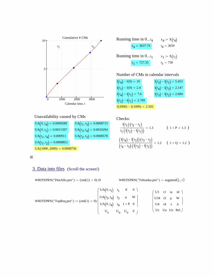
I t2( ) I t1( )− 2.769=
I 2000( ) I 1000( )− 2.502=
Unavailability caused by CMs Checks:
I t1( ) t2 t1−( )⋅
t1 I t2( ) I t1( )−( )⋅1.3=
( 1 P+ 1.3= )
I t4( ) I t3( )−( ) t3 t2−( )⋅
t4 t3−( ) I t3( ) I t2( )−( )⋅1.2= ( 1 Q+ 1.2= )
UA 0 t4,( ) 0.0009589= UA t1 t3,( ) 0.0008715=
UA 0 t1,( ) 0.0011507= UA t3 t4,( ) 0.0010294=
UA t1 t4,( ) 0.000911= UA t2 t3,( ) 0.0008578=
UA t1 t2,( ) 0.0008851=
UA 1000 2000,( ) 0.0008756=
3. Data into files (Scroll the screen!)
WRITEPRN "DistAllo.prn"( ) rnd 1( ) 0>( ) D⋅:= WRITEPRN "Tehoaika.prn"( ) augment ξ τ,( ):=
WRITEPRN "TopReq.prn"( ) rnd 1( ) 0>( )
UA 0 t1,( )UA t3 t4,( )UA 0 t4,( )
Us
t1
t3
t4
Uu
0
μ
1 P+
Uo
0
W
0
0
⎛⎜⎜⎜⎜⎜⎝
⎞⎟⎟⎟⎟⎟⎠
⋅:=
U1
U34
U4
Us
t1
t3
t4
Uu
ta
μ
s
Uo
td
W
Δ
Rel
⎛⎜⎜⎜⎜⎝
⎞⎟⎟⎟⎟⎠
0 1000 2000 3000
5
10Cumulative # CMs
Calendar time, t
t1 t3
Running time in 0... t4 x4 X t4( ):=
x4 3637.74= t4 3650=
Running time in 0... t1 x1 X t1( ):=
x1 727.35= t1 730=
Number of CMs in calendar intervalsI t4( ) I 0( )− 10= I t3( ) I t1( )− 5.453=
I t1( ) I 0( )− 2.4= I t4( ) I t3( )− 2.147=
I t4( ) I t1( )− 7.6= I t3( ) I t2( )− 2.684=

minimum single CM-timeσ 0.07:= standard deviation of single CM-time
0.25 0.3 0.35 0.4 0.45 0.5 0.55
0.20.40.60.8
1Cdf for CM-time
μ T 0.95( )P-quantile T 0.95( ) 0.486=
2. Required reliability (CM) in calendar interval 0... t4 3650=
ta 1 365⋅:= td 9 365⋅:= main interval ta...td containing t1 730= & t3 2920=
Δ 61:= Rel 0.84:= reliability (CM) in periods of length Δ during interval ta...td
more CMs allowed in 0... t1 than in t1...2t1
P 20 %⋅:= Δ td ta−< λ0ln Rel( )−
Δ:=
ta Δ+ 2 t1⋅< td Δ−<λ0 0.002858=
λ 0.9 λ0⋅:= minimal CM rate at 2 t1 (λ < λ0)0 ta< t1≤ t3< td≤ t4≤
λ 0.002572=γ 5:= shape after 2.t1 γ 2≥
l i
Kommentit: [email protected]
D rnd 1( ) 0>( ) READPRN "DistAllo.prn"( )⋅:= PRNPRECISION 10:= δ 0.0001:= i 1 400..:=
AT rnd 1( ) 0>( ) READPRN "AT.prn"( )⋅:= PRNCOLWIDTH 16:= Z t( ) t 0≥( ) t⋅:=
TOP AT0 cols AT( ) 1−,:=
1. Basic data and requirements for TOP 12=
t4 10 365⋅:= total (calendar) time 0... t4 t4 3650=
t1 2 365⋅:= beginning period 0... t1 t1 730= 0 t1< t3< t4<
t3 8 365⋅:= wear-out period t3... t4 t3 2920=
Us 0.001:= unavailability caused by SPM (scheduled PM) Unavailability except CMUu 0.0004:= unavailability caused by UPM (unscheduled PM)
Uo 0.001:= unavailability other than SPM, UPM, CM Us Uu+ Uo+ 0.0024=
μ 0.35:= average single CM-time a 0.25:=

UA 0 t1,( ) 0.0010824= UA ta td,( ) 0.0009202=
I ta( ) I 0( )− 1.268= I t4( ) I td( )− 1.105= UA 0 ta,( ) 0.001216= UA td t4,( ) 0.0010595=
I 2000( ) I 1000( )− 2.573= UA 1000 2000,( ) 0.0009005=
e I td( ) I td Δ−( )−( )− 0.84=Checks I t1( )
I 2 t1⋅( ) I t1( )−1.2= ( 1 P+ 1.2= , Rel 0.84= )
e I ta Δ+( ) I ta( )−( )− 0.8400106=
3. Data into files (Scroll the screen!)
WRITEPRN "DistAllo.prn"( ) rnd 1( ) 0>( ) D⋅:= WRITEPRN "Tehoaika.prn"( ) augment ξ τ,( ):=
WRITEPRN "TopReq.prn"( ) rnd 1( ) 0>( )
UA 0 t1,( )UA t3 t4,( )UA 0 t4,( )
Us
t1
t3
t4
Uu
ta
μ
1 P+
Uo
td
W
Δ
Rel
⎛⎜⎜⎜⎜⎜⎝
⎞⎟⎟⎟⎟⎟⎠
⋅:=
U1
U34
U4
Us
t1
t3
t4
Uu
ta
μ
s
Uo
td
W
Δ
Rel
⎛⎜⎜⎜⎜⎝
⎞⎟⎟⎟⎟⎠
0 1000 2000 3000
0.002
0.004
0.006CM rate
Calendar time, t
ta td
0 1000 2000 3000
5
10
15Cumulative # CMs
Calendar time, t
ta td
0 1000 2000 3000
0.001
0.002Unavailability caused by CMs
Calendar time, t
t1 2 t1⋅Running time in 0...t4 x4 X t4( ):=
x4 3637.723= t4 3650=
Running time in 0...t1 x1 X t1( ):=
x1 727.422= t1 730=
Number of CMs in calendar intervals Unavailability caused by CMsI t4( ) I 0( )− 10.05= I t4( ) I t1( )− 7.792= UA 0 t4,( ) 0.0009637= UA t1 t4,( ) 0.000934=
I t1( ) I 0( )− 2.258= I td( ) I ta( )− 7.677=
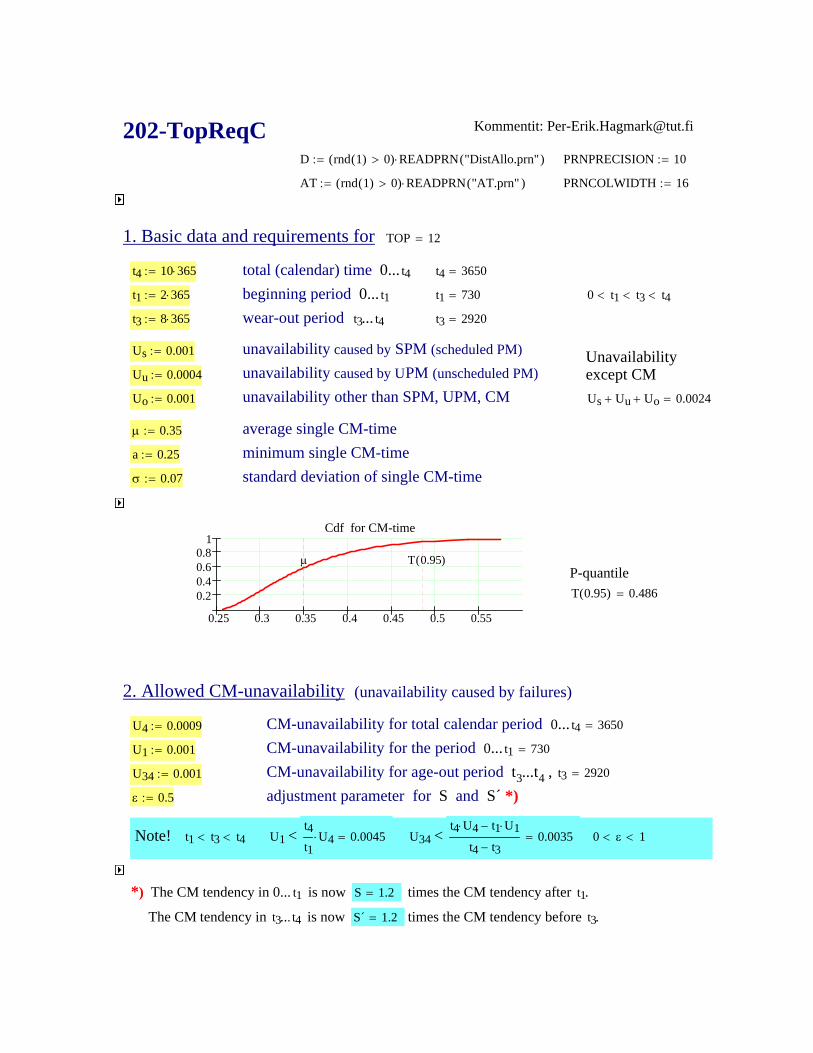
Us Uu+ Uo+ 0.0024=
μ 0.35:= average single CM-time a 0.25:= minimum single CM-timeσ 0.07:= standard deviation of single CM-time
0.25 0.3 0.35 0.4 0.45 0.5 0.55
0.20.40.60.8
1Cdf for CM-time
μ T 0.95( )P-quantile T 0.95( ) 0.486=
2. Allowed CM-unavailability (unavailability caused by failures)
U4 0.0009:= CM-unavailability for total calendar period 0... t4 3650=
U1 0.001:= CM-unavailability for the period 0... t1 730= U34 0.001:= CM-unavailability for age-out period t3...t4 , t3 2920=
ε 0.5:= adjustment parameter for S and S´ *)
Note! t1 t3< t4< U1 < t4t1
U4⋅ 0.0045= U34 < t4 U4⋅ t1 U1⋅−
t4 t3−0.0035= 0 ε< 1<
*) The CM tendency in 0... t1 is now S 1.2= times the CM tendency after t1. The CM tendency in t3... t4 is now S´ 1.2= times the CM tendency before t3.
Kommentit: [email protected] rnd 1( ) 0>( ) READPRN "DistAllo.prn"( )⋅:= PRNPRECISION 10:=
AT rnd 1( ) 0>( ) READPRN "AT.prn"( )⋅:= PRNCOLWIDTH 16:=
1. Basic data and requirements for TOP 12=
t4 10 365⋅:= total (calendar) time 0... t4 t4 3650=
t1 2 365⋅:= beginning period 0... t1 t1 730= 0 t1< t3< t4<
t3 8 365⋅:= wear-out period t3... t4 t3 2920=
Us 0.001:= unavailability caused by SPM (scheduled PM) Unavailability except CMUu 0.0004:= unavailability caused by UPM (unscheduled PM)
Uo 0.001:= unavailability other than SPM, UPM, CM

I t4( ) I 0( )− 9.386= I t3( ) I t1( )− 5.214= UA 0 t4,( ) 0.0009= UA t1 t3,( ) 0.0008333=
I t1( ) I 0( )− 2.086= I t4( ) I t3( )− 2.086= UA 0 t1,( ) 0.001= UA t3 t4,( ) 0.001=
I t4( ) I t1( )− 7.3= UA t1 t4,( ) 0.000875=
I 2000( ) I 1000( )− 2.384= UA 1000 2000,( ) 0.0008344=
3. Data into files (Scroll the screen!)
WRITEPRN "DistAllo.prn"( ) rnd 1( ) 0>( ) D⋅:= WRITEPRN "Tehoaika.prn"( ) augment ξ τ,( ):=
WRITEPRN "TopReq.prn"( ) rnd 1( ) 0>( )
UA 0 t1,( )UA t3 t4,( )UA 0 t4,( )
Us
t1
t3
t4
Uu
0
μ
S
Uo
0
W
0
0
⎛⎜⎜⎜⎜⎜⎝
⎞⎟⎟⎟⎟⎟⎠
⋅:=
0 1000 2000 3000
0.002
0.004CM rate
Calendar time, t
t1 t3
0 1000 2000 3000
5
10Cumulative # CMs
Calendar time, t
t1 t3
0 1000 2000 3000
0.001
0.002Unavailability caused by CMs
Calendar time, t
t1 t3
Running time in 0...t4 x4 X t4( ):= x4 3637.955= t4 3650=
Running time in 0...t1 x1 X t1( ):= x1 727.486= t1 730=
Running time in 0...t3 x3 X t3( ):= x3 2910.469= t3 2920=
Number of CMs in calendar intervals Unavailability caused by CMs

AT
14
2
2
0.95
15
2
0
12
1
2
1
14
7
0
⎛⎜⎜⎜⎜⎜⎜⎜⎜⎝
⎞⎟⎟⎟⎟⎟⎟⎟⎟⎠
=
Gate
AtLeast
AtMost
CondProb
Input1
Input2
....
⎛⎜⎜⎜⎜⎜⎜⎜⎜⎜⎝
⎞⎟⎟⎟⎟⎟⎟⎟⎟⎟⎠
Allocation tree to be considered next
The allocation tree should consist of the column for the gate to be allocated now and the already allocated columns.
ET p⟨ ⟩ChangedET p⟨ ⟩
14
2
2
0.95
15
2
0
⎛⎜⎜⎜⎜⎜⎜⎜⎜⎝
⎞⎟⎟⎟⎟⎟⎟⎟⎟⎠
=
Gate
AtLeast
AtMost
CondProb
Input1
Input2
....
⎛⎜⎜⎜⎜⎜⎜⎜⎜⎜⎝
⎞⎟⎟⎟⎟⎟⎟⎟⎟⎟⎠
The type of Gate 14= (i.e. AtLeast, AtMost, CondProb) can be redefined.
p Pos Gate ETT( ) 0⟨ ⟩,
⎡⎣
⎤⎦:=Gate 14:=The gate to be allocated now?
ET
2
2
3
0.7
3
10
5
12
1
2
1
14
7
0
14
2
2
0.95
15
2
0
⎛⎜⎜⎜⎜⎜⎜⎜⎜⎝
⎞⎟⎟⎟⎟⎟⎟⎟⎟⎠
=
Gate
AtLeast
AtMost
CondProb
Input1
Input2
....
⎛⎜⎜⎜⎜⎜⎜⎜⎜⎜⎝
⎞⎟⎟⎟⎟⎟⎟⎟⎟⎟⎠
Entire tree (defined in201-NewAllo)
1. Preparation of allocation tree for CM with TOP 12=
PRNPRECISION 10:=AT READPRN "AT.prn"( ):=I READPRN "AID.prn"( ):=
PRNCOLWIDTH 16:=ET READPRN "Puu.prn"( ):=
203. AlloTree Kommentit: [email protected]
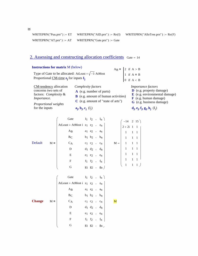
MM
Gate
AtLeast AtMost i⋅+
AB
BC
CA
D
E
F
G
I1
z1
a1
b1
c1
d1
e1
f1
g1
I2
z2
a2
b2
c2
d2
e2
f2
g2
..
..
..
..
..
..
..
..
..
In
zn
an
bn
cn
dn
en
fn
gn
⎛⎜⎜⎜⎜⎜⎜⎜⎜⎜⎜⎜⎜⎜⎝
⎞⎟⎟⎟⎟⎟⎟⎟⎟⎟⎟⎟⎟⎟⎠
=Change
M
14−
2 2i+
1
1
1
1
1
1
1
2
1
1
1
1
1
1
1
1
15
1
1
1
1
1
1
1
1
⎛⎜⎜⎜⎜⎜⎜⎜⎜⎜⎜⎜⎝
⎞⎟⎟⎟⎟⎟⎟⎟⎟⎟⎟⎟⎠
=M
Gate
AtLeast AtMost i⋅+
AB
BC
CA
D
E
F
G
I1
z1
a1
b1
c1
d1
e1
f1
g1
I2
z2
a2
b2
c2
d2
e2
f2
g2
..
..
..
..
..
..
..
..
..
In
zn
an
bn
cn
dn
en
fn
gn
⎛⎜⎜⎜⎜⎜⎜⎜⎜⎜⎜⎜⎜⎜⎝
⎞⎟⎟⎟⎟⎟⎟⎟⎟⎟⎟⎟⎟⎟⎠
=Default
dj, ej, fj, gj, hj (Ij) aj, bj, cj (Ij)Proportional weights for the inputs
Importance factors D (e.g. property damage) E (e.g. environmental damage) F (e.g. human damage) G (e.g. business damage)
Complexity factors A (e.g. number of parts) B (e.g. amount of human activities) C (e.g. amount of "state of arts")
CM-tendency allocationconcerns two sets offactors: Complexity &Importance.
AB 2 A B>if
1 A B=if
0 A B<if
=Instructions for matrix M (below)
Type of Gate to be allocated: AtLeast 1− AtMost⋅+ Proportional CM-time zj for inputs Ij
2. Assessing and constructing allocation coefficients Gate 14=
WRITEPRN "Gate.prn"( ) Gate:=WRITEPRN "AT.prn"( ) AT:=
WRITEPRN "AlloTree.prn"( ) Re F( ):=WRITEPRN "AID.prn"( ) Re I( ):=WRITEPRN "Puu.prn"( ) ET:=
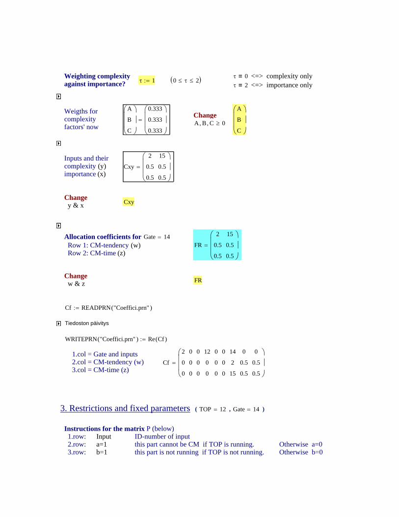
Instructions for the matrix P (below) 1.row: Input ID-number of input 2.row: a=1 this part cannot be CM if TOP is running. Otherwise a=0 3.row: b=1 this part is not running if TOP is not running. Otherwise b=0
3. Restrictions and fixed parameters ( TOP 12= , Gate 14= )
Cf
2
0
0
0
0
0
0
0
0
12
0
0
0
0
0
0
0
0
14
2
15
0
0.5
0.5
0
0.5
0.5
⎛⎜⎜⎜⎝
⎞⎟⎟⎟⎠
=1.col = Gate and inputs2.col = CM-tendency (w)3.col = CM-time (z)
WRITEPRN "Coeffici.prn"( ) Re Cf( ):=
Tiedoston päivitys
Cf READPRN "Coeffici.prn"( ):=
FRChange w & z
FR
2
0.5
0.5
15
0.5
0.5
⎛⎜⎜⎜⎝
⎞⎟⎟⎟⎠
=Allocation coefficients for Gate 14= Row 1: CM-tendency (w) Row 2: CM-time (z)
CxyChange y & x
Cxy
2
0.5
0.5
15
0.5
0.5
⎛⎜⎜⎜⎝
⎞⎟⎟⎟⎠
=Inputs and theircomplexity (y)importance (x)
A
B
C
⎛⎜⎜⎜⎝
⎞⎟⎟⎟⎠
A
B
C
⎛⎜⎜⎜⎝
⎞⎟⎟⎟⎠
0.333
0.333
0.333
⎛⎜⎜⎜⎝
⎞⎟⎟⎟⎠
=ChangeA B, C 0≥,
Weigths forcomplexity factors' now
0 τ≤ 2≤( )τ 1:=τ 0= <=> complexity only τ 2= <=> importance only
Weighting complexity against importance?
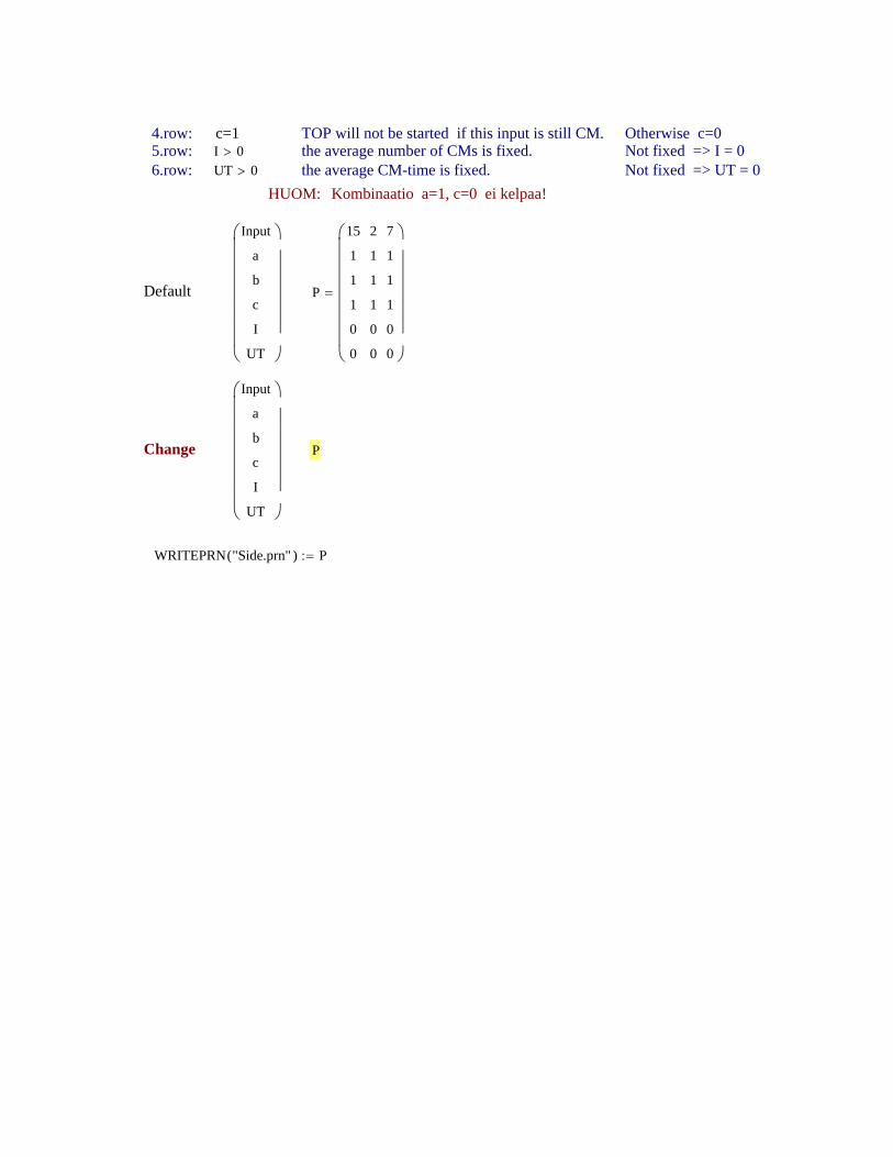
4.row: c=1 TOP will not be started if this input is still CM. Otherwise c=0 5.row: I 0> the average number of CMs is fixed. Not fixed => I = 0 6.row: UT 0> the average CM-time is fixed. Not fixed => UT = 0 HUOM: Kombinaatio a=1, c=0 ei kelpaa!
Default
Input
a
b
c
I
UT
⎛⎜⎜⎜⎜⎜⎜⎜⎝
⎞⎟⎟⎟⎟⎟⎟⎟⎠
P
15
1
1
1
0
0
2
1
1
1
0
0
7
1
1
1
0
0
⎛⎜⎜⎜⎜⎜⎜⎜⎝
⎞⎟⎟⎟⎟⎟⎟⎟⎠
=
Change
Input
a
b
c
I
UT
⎛⎜⎜⎜⎜⎜⎜⎜⎝
⎞⎟⎟⎟⎟⎟⎟⎟⎠
P
WRITEPRN "Side.prn"( ) P:=

WRITEPRN "Events.prn"( ) Ev:=
WRITEPRN "DistAllo.prn"( ) CT:=0 1000 2000 3000
5
10
Simulated Required
Cumulative # CMs
Calendar time
t1 t3
Raw simulation data
Allocation, simulation, etc. Simuloinnin toisto: Klikkaa N ja F9!N 1000:=Number of copies
β 0.9:=Level parameter for CM timeBigger α => more CM tendencyBigger β => longer CM time(Begin with α = 1, β = 1.)
α 4:=Level parameter for CM tendency
AT
14
2
2
0.95
15
2
0
12
1
2
1
14
7
0
⎛⎜⎜⎜⎜⎜⎜⎜⎜⎝
⎞⎟⎟⎟⎟⎟⎟⎟⎟⎠
=
Gate
AtLeast
AtMost
CondProb
Input1
Input2
....
⎛⎜⎜⎜⎜⎜⎜⎜⎜⎜⎝
⎞⎟⎟⎟⎟⎟⎟⎟⎟⎟⎠
Allocation treeto be simulated
204-AlloSim Kommentit: [email protected] PRNCOLWIDTH 16:=
PRNPRECISION 10:=Cf READPRN "Coeffici.prn"( ):= ET READPRN "Puu.prn"( ):=P READPRN "Side.prn"( ):=Gate READPRN "Gate.prn"( )0 0,:= TR READPRN "TopReq.prn"( ):=F READPRN "AlloTree.prn"( ):=ID READPRN "AID.prn"( ):= D READPRN "DistAllo.prn"( ):=AT READPRN "AT.prn"( ):=xt READPRN "Tehoaika.prn"( ):= A READPRN "SumParts.prn"( ):=
1. Allocating distributions for inputs (Gate 14= ) and simulation (to TOP 12= )
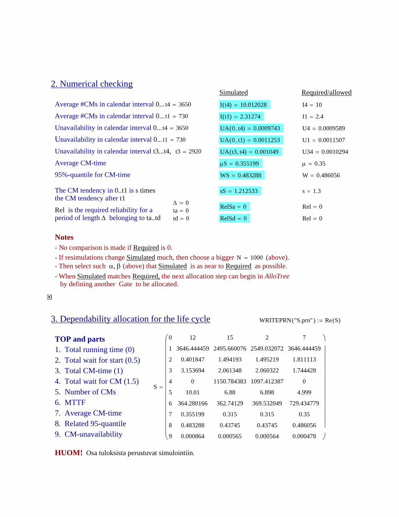
95%-quantile for CM-time WS 0.483288= W 0.486056=
The CM tendency in 0..t1 is s times the CM tendency after t1
sS 1.212533= s 1.3=
Δ 0= RelSa 0= Rel 0=Rel is the required reliability for a period of length Δ belonging to ta..td
ta 0=td 0= RelSd 0= Rel 0=
Notes - No comparison is made if Required is 0. - If resimulations change Simulated much, then choose a bigger N 1000= (above). - Then select such α, β (above) that Simulated is as near to Required as possible. - When Simulated matches Required, the next allocation step can begin in AlloTree by defining another Gate to be allocated.
3. Dependability allocation for the life cycle WRITEPRN "S.prn"( ) Re S( ):=
TOP and parts 1. Total running time (0) 2. Total wait for start (0.5) 3. Total CM-time (1) 4. Total wait for CM (1.5) 5. Number of CMs 6. MTTF 7. Average CM-time 8. Related 95-quantile 9. CM-unavailability
S
0
1
2
3
4
5
6
7
8
9
12
3646.444459
0.401847
3.153694
0
10.01
364.280166
0.355199
0.483288
0.000864
15
2495.660076
1.494193
2.061348
1150.784383
6.88
362.74129
0.315
0.43745
0.000565
2
2549.032072
1.495219
2.060322
1097.412387
6.898
369.532049
0.315
0.43745
0.000564
7
3646.444459
1.811113
1.744428
0
4.999
729.434779
0.35
0.486056
0.000478
⎛⎜⎜⎜⎜⎜⎜⎜⎜⎜⎜⎜⎜⎜⎝
⎞⎟⎟⎟⎟⎟⎟⎟⎟⎟⎟⎟⎟⎟⎠
=
HUOM! Osa tuloksista perustuvat simulointiin.
2. Numerical checkingSimulated Required/allowed
Average #CMs in calendar interval 0... t4 3650= I t4( ) 10.012028= I4 10=
Average #CMs in calendar interval 0... t1 730= I t1( ) 2.31274= I1 2.4=
Unavailability in calendar interval 0... t4 3650= UA 0 t4,( ) 0.0009743= U4 0.0009589=
Unavailability in calendar interval 0... t1 730= UA 0 t1,( ) 0.0011253= U1 0.0011507=
Unavailability in calendar interval t3...t4, t3 2920= UA t3 t4,( ) 0.001049= U34 0.0010294=
Average CM-time μS 0.355199= μ 0.35=

Gates 1. total CM-time 2. number of failures
G
0
1
2
14
1.4573341
5.185
12
3.1536942
10.01
⎛⎜⎜⎜⎝
⎞⎟⎟⎟⎠
=
4. Dependability allocation for selected interval
Interval: T0 T1( ) 2 365⋅ 7 365⋅( ):= SPV T0 T1 1−⋅+ 0≠( ) READPRN "SumParts.prn"( )⋅:=
SPV0 cols SP( ) 1−, 0:= WRITEPRN "SumParts.prn"( ) stack SPV SP,( ):=
TOP and parts 0 calendar interval T0-T1i1 number of the part (entity) ID 2 average # CMs I3 95% quantile for # CMs Iw4 reliability (no CMs) R 5 CM-unavailability U6 average single CM-time m
SP
0 1 2 30123456
730-2555i 730-2555i 730-2555i 730-2555i12 15 2 7
4.622 4.560179 4.560179 2.280098.400035 8.315182 8.315182 4.9915130.009833 0.01046 0.01046 0.102275
0.0009 0.000787 0.000787 0.0004370.355199 0.315 0.315 0.35
=
HUOM! Osa tuloksista perustuvat simulointiin.

Parts BPT 15 2 7( )=
Average #CMs (AlloSim) IT 4.56 4.56 2.28( )=
Average single CM-time (TopReq) μT
0.315 0.315 0.35( )=
TOP-yksikkö TOP 12=
Tarkasteltava kalenteriaikaväli T0 T1( ) 730 2555( )=
TOP:n CM-epäkäytettävyys (AlloSim) Uc 0.0009=TOP:n CM-epäkäytettävyysaika Uc T1 T0−( )⋅ 1.641729=
TOP:n UPM-epäkäytettävyys (TopReq) ω Uc⋅ 0.000375= ω 0.417=TOP:n UPM-epäkäytettävyysaika ω Uc⋅ T1 T0−( )⋅ 0.684836=
TOP:n SPM-epäkäytettävyys (TopReq) Us 0.001=TOP:n SPM-epäkäytettävyysaika Us T1 T0−( )⋅ 1.825=
TOP:n Muu epäkäytettävyys (TopReq) Uo 0.001=TOP:n Muu epäkäytettävyysaika Uo T1 T0−( )⋅ 1.825=
TOP:n koko epäkäytettävyys U 0.003275=TOP:n koko epäkäytettävyysaika U T1 T0−( )⋅ 5.976565=
Osa tuloksista perustuvat simulointiin, joten voi esiintyä pieniä ristiriitoja, jotka pienenevät kun simulointimääriä lisätään (AlloSim).
SP
0 1 2 30123456
730-2555i 730-2555i 730-2555i 730-2555i12 15 2 7
4.622 4.560179 4.560179 2.280098.400035 8.315182 8.315182 4.9915130.009833 0.01046 0.01046 0.102275
0.0009 0.000787 0.000787 0.0004370.355199 0.315 0.315 0.35
=
Viimeinen simuloitu tapaus
0. Calendar interval (T0-T1i) 1. Part's ID-number 2. Average # CMs 3. 95% quantile for # CMs 4. Reliability (no CMs) 5. CM-unavailability 6. Average single CM-time
1. Initial results (from TopReq and AlloSim)
TR READPRN "TopReq.prn"( ):=SPV READPRN "SumParts.prn"( ):=ID READPRN "AID.prn"( ):=
xt READPRN "Tehoaika.prn"( ):=D READPRN "DistAllo.prn"( ):=PRNCOLWIDTH 16:=
PRNPRECISION 10:=Kommentit: [email protected]

z 0:=Huoltojen päällekkäisyys 2)δ 0.5 0 1( )T:=
1)TOP:n pysähdystarve osan huollon aikana
β21
11
43
⎛⎜⎝
⎞⎟⎠
T:=
Kustannussuhde 'materiaali/työ' kullekin osalle
θ 2 1 1.5( )T:=Työn suhteellinen hinta /ay osille
γ 1 2 1( )T:=Työajan suht. allokointikertoimet osille
BPT 15 2 7( )=Parts
(material + työ)Cu 5000:=UPM-costs allowed (material + work)
3. UPM cost and time allocation T0 T1( ) 730 2555( )=
CM-kustannukset yhteensä (eu) Σ kt Σ km+ 8000.00= (vrt. Cc)
Työn kustannus (eu) Σ kt 3563.03=
Materiaalikustannus(eu) Σ km 4436.97=
Työkustannusten osuus X 44.5%=
Työaikaa osille (ay) (AlloSim)
I μ⋅( )→⎯⎯T
1.436 1.436 0.798( )=
Työn hinta (eu/ay) d κT
⋅ 842.41 1263.61 673.93( )=
Materiaalin hinta (eu/CM) d mT⋅ 530.72 265.36 353.81( )=
CM-kustannukset osille (eu) ktT kmT+ 3630.25 3025.21 1344.54( )=
Työn kustannus (eu) ktT 1210.08 1815.13 537.82( )=
Materiaalikustannus (eu) kmT 2420.17 1210.08 806.72( )=
α21
11.5
32
⎛⎜⎝
⎞⎟⎠
T:=
Kustannussuhde 'materiaali/työ' kullekin osalle
κ 1 1.5 0.8( )T:=Työn suhteellinen hinta /ay osille
BPT 15 2 7( )=Parts
Cc 8000:=CM-costs allowed (material + work)
2. CM cost and time allocation T0 T1( ) 730 2555( )=
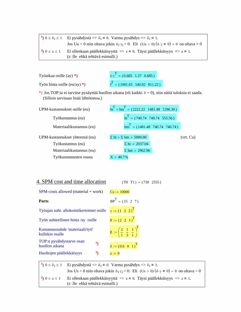
1) 0 δi≤ 1≤ Ei pysähdystä => δi 0= . Varma pysähdys => δi 1= . Jos Us > 0 niin oltava jokin δi γ i⋅ > 0. Eli Us 0>( ) δ γ⋅ 0=( )⋅ 0= on oltava = 0
2) 0 z≤ 1≤ Ei ollenkaan päällekkäisyyttä => z 0= . Täysi päällekkäisyys => z 1= .(z :lle ehkä tehtävä esimalli.)
z 0:=Huoltojen päällekkäisyys 2)δ 0.6 0 1( )T:=
1)TOP:n pysähdystarve osan huollon aikana
β21
13
11
⎛⎜⎝
⎞⎟⎠
T:=
Kustannussuhde 'materiaali/työ' kullekin osalle
θ 2 2 1( )T:=Työn suhteellinen hinta /ay osille
γ 1 2 2( )T:=Työajan suht. allokointikertoimet osille
BPT 15 2 7( )=Parts
Cs 10000:=SPM-costs allowed (material + work)
4. SPM cost and time allocation T0 T1( ) 730 2555( )=
UPM-kustannukset yhteensä (eu) Σ ht Σ hm+ 5000.00= (vrt. Cu)
Työkustannus (eu) Σ ht 2037.04=
Materiaalikustannus (eu) Σ hm 2962.96=
Työkustannusten osuus X 40.7%=
Työaikaa osille (ay) *) c γT
⋅ 0.685 1.37 0.685( )=
Työn hinta osille (eu/ay) *) fT 1081.63 540.82 811.22( )=
*) Jos TOP:ia ei tarvitse pysäyttää huollon aikana (eli kaikki δ = 0), niin näitä tuloksia ei saada. (Silloin tarvitaan lisää lähtötietoa.)
UPM-kustannukset osille (eu) htT hmT+ 2222.22 1481.48 1296.30( )=
Työkustannus (eu) htT 740.74 740.74 555.56( )=
Materiaalikustannus (eu) hmT 1481.48 740.74 740.74( )=
1) 0 δi≤ 1≤ Ei pysähdystä => δi 0= . Varma pysähdys => δi 1= . Jos Uu > 0 niin oltava jokin δi γ i⋅ > 0. Eli Uu 0>( ) δ γ⋅ 0=( )⋅ 0= on oltava = 0
2) 0 z≤ 1≤ Ei ollenkaan päällekkäisyyttä => z 0= . Täysi päällekkäisyys => z 1= .(z :lle ehkä tehtävä esimalli.)

Työaikaa osille (ay) *) c γT
⋅ 0.913 1.825 1.825( )=
Työn hinta osille (eu/ay) *) fT 1429.42 1429.42 714.71( )=
*) Jos TOP:ia ei tarvitse pysäyttää huollon aikana (eli kaikki δ = 0), niin näitä tuloksia ei saada. (Silloin tarvitaan lisää lähtötietoa.)
SPM-kustannukset osille (eu) htT hmT+ 3913.04 3478.26 2608.70( )=
Työkustannus (eu) htT 1304.35 2608.70 1304.35( )=
Materiaalikustannus (eu) hmT 2608.70 869.57 1304.35( )=
SPM-kustannukset yhteensä (eu) Σ ht Σ hm+ 10000.00= (vrt. Cs)
Työkustannus (eu) Σ ht 5217.39=
Materiaalikustannus (eu) Σ hm 4782.61=
Työkustannusten osuus X 52.2%=
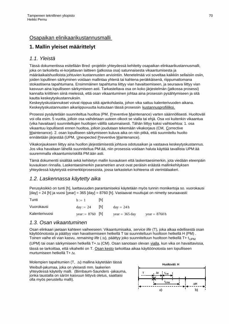
Tampereen teknillinen yliopistoHeikki Pernu
70
Molempien tapahtumien (T, Δt) mallina käytetään tässä Weibull-jakumaa, joka on yleisesti mm. laakerien yhteydessä käytetty malli. (Birnbaum-Saunders -jakauma, jonka taustalla on särön kasvuun liittyvä oletus, saattaisi olla myös perusteltu malli).
a) b)
ΔH
Δt
tUPM
T tCM
Huoltoväli: H
a) b)
ΔH
Δt
tUPM
T tCM
Huoltoväli: H
Osan elinkaari jaetaan kahteen vaiheeseen: Vikaantumisaika, service life (T), joka alkaa edellisestä osan käyttöönotosta ja päättyy vian havaitsemiseen hetkellä T tai suunniteltuun huoltoon hetkellä H (PM) . Toinen vaihe eli vian kasvu, remaining life (Δt), päättyy joko suunniteltuun huoltoon hetkellä T+ tUPM (UPM) tai osan särkymiseen hetkellä T+ Δt (CM). Osan sanotaan olevan vialla, kun vika on havaittavissa, tässä se tarkoittaa, että vikahetki on T. Osan kesto tarkoittaa aikaa käyttöönotosta sen lopulliseen murtumiseen hetkellä T+Δt.
1.3. Osan vikaantuminen
year 8760 h=year 365 day=[h]year 8760:=Kalenterivuosi
day 24 h=[h]day 24:=Vuorokausi
[h]h 1:=Tunti
Perusyksikkö on tunti [h], luettavuuden parantamiseksi käytetään myös tunnin monikertoja so. vuorokausi [day] = 24 [h] ja vuosi [year] = 365 [day] = 8760 [h]. Vastaavat muuttujat on nimetty seuraavasti:
1.2. Laskennassa käytetty aika
Tämä dokumentti sisältää sekä kehitetyn mallin kuvauksen että laskentaesimerkin, jota viedään eteenpäin kuvauksen rinnalla. Laskentaesimerkin parametrien arvot ovat peräisin eräästä mallinkehityksen yhteydessä käytetystä esimerkkiprosessista, jossa tarkastelun kohteena oli vierintälaakeri.
Vikakorjaukseen liittyy aina huollon järjestämisestä johtuva odotusaikan ja vastaava keskeytyskustannus. Jos vika havaitaan lähellä suunniteltua PM:ää, niin prosessia voidaan haluta käyttää tavallista UPM:ää suuremmalla vikaantumisriskillä PM:ään asti.
Prosessi pysäytetään suunniteltua huoltoa (PM, Preventive Maintenance) varten säännöllisesti. Huoltoväli voi olla esim. 5 vuotta, jolloin osa vaihdetaan uuteen olkoot se vialla tai ehjä. Osa voi kuitenkin vikaantua (vika havaitaan) suunniteltujen huoltojen välillä satunnaisesti. Tähän liittyy kaksi vaihtoehtoa: 1. osa vikaantuu lopullisesti ennen huoltoa, jolloin joudutaan tekemään vikakorjaus (CM, Corrective Maintenance). 2. osan lopulliseen särkymiseen kuluva aika on niin pitkä, että suunniteltu huolto ennätetään järjestää (UPM, Unexpected Preventive Maintenance).
Tässä dokumentissa esitellään Bred -projektin yhteydessä kehitetty osapaikan elinkaarikustannusmalli, joka on tarkoitettu ei-korjattavan laitteen (jatkossa osa) satunnaisesta vikaantumisesta ja määräaikaishuolloista johtuvien kustannusten arviointiin. Menetelmää voi soveltaa kaikkiin sellaisiin osiin, joiden lopullinen särkyminen voidaan mallintaa yhtenä tai kahtena peräkkäisenä, riippumattomana stokastisena tapahtumana. Ensimmäinen tapahtuma liittyy vian havaitsemiseen, ja seuraava liittyy vian kasvuun aina lopulliseen särkymiseen asti. Tarkasteltava osa on koko järjestelmän (jatkossa prosessi) kannalta kriittinen siinä mielessä, että osan vikaantuminen johtaa aina prosessin pysähtymiseen ja sitä kautta keskeytyskustannuksiin.Keskeytyskustannukset voivat riippua siitä ajankohdasta, johon vika sattuu kalenterivuoden aikana. Keskeytyskustannusten aikariippuvuutta kutsutaan tässä prosessin kustannusprofiiliksi.
1.1. Yleistä
1. Mallin yleiset määrittelyt
Osapaikan elinikaarikustannusmalli

Tampereen teknillinen yliopistoHeikki Pernu
71
1.4. Osan kunnossapitostrategiaKunnossapitostrategian perusperiaatteita:Vika havaitaan aikavälillä a:Osa vaihdetaan hetkellä ..T+ tUPM (UPM). Jos osa särkyy lopullisesti ennen hetkeä ..T+ tUPM, niin seuraa vikakorjaus (CM) hetkellä ..T+Δt + tCM. tCM on korjauksen odotusaika
Vika havaitaan aikavälillä b:Osa vaihdetaan huoltovälin H lopussa (PM).Särkymisestä hetkellä ..T+Δt < H seuraa vikakorjaus (CM) hetkellä ..T+Δt + tCM. a) b)
ΔH
Δt
tUPM
T tCM
Huoltoväli: H
a) b)
ΔH
Δt
tUPM
T tCM
Huoltoväli: H
Osa (ehjä tai rikki) vaihdetaan aina huoltovälin H lopussa (PM). ..T on vian havaitsemisajankohta mitattuna huoltovälin H alusta ja tCM = max[(varaosan toimitusaika – Δt), huollon järjestämisaika].
1.5. Prosessin (osan) käyttö- ja kustannusprofiili
Käyttöprofiili kuvaa prosessin keskimääräistä käyttömäärää (käyttötunteja) kalenterivuoden eri ajanjaksoina. Kustannusprofiili kuvaa vastaaviin jaksoihin liittyviä keskeytyskustannuksia.
Esimerkkiprosessimme käy yhteensä 6000 h vuodessa. Käyttöprofiili on seuraava:Vuosi on jaettu neljään jaksoon, jotka on tässä numeroitu 0-3. Käyttöjaksojen kestot ovat likimääräisiä ja ne tarkentuvat parametrien kiinnityksen yhteydessä alempana.
Käyttöjakso 0: Käyntiaika 500h, viasta johtuva keskeytyskustannus 22k€/h Käyttöjakso 1: Käyntiaika 3500h, viasta johtuva keskeytyskustannus 44k€/h Käyttöjakso 2: Käyntiaika 1000h, viasta johtuva keskeytyskustannus 30k€/h Käyttöjakso 3: Käyntiaika 1000h, viasta johtuva keskeytyskustannus 30k€/h
Kuva 1. Prosessin (osan) käyttöprofiili. Kuvassa on esitetty kalenterivuosi, joka alkaa 31. päivä maaliskuuta. Käyttöjaksot (rpd) on numeroitu 0...3.
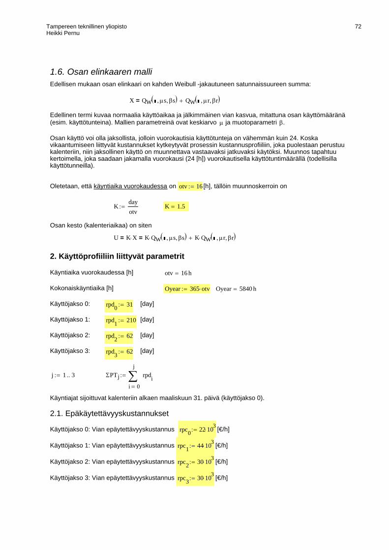
Tampereen teknillinen yliopistoHeikki Pernu
72
rpd0 31:= [day]
Käyttöjakso 1: rpd1 210:= [day]
Käyttöjakso 2: rpd2 62:= [day]
Käyttöjakso 3: rpd3 62:= [day]
j 1 3..:= ΣPTj
0
j
i
rpdi∑=
:=
Käyntiajat sijoittuvat kalenteriin alkaen maaliskuun 31. päivä (käyttöjakso 0).
2.1. Epäkäytettävyyskustannukset
Käyttöjakso 0: Vian epäytettävyyskustannus rpc0 22 103⋅:= [€/h]
Käyttöjakso 1: Vian epäytettävyyskustannus rpc1 44 103⋅:= [€/h]
Käyttöjakso 2: Vian epäytettävyyskustannus rpc2 30 103⋅:= [€/h]
Käyttöjakso 3: Vian epäytettävyyskustannus rpc3 30 103⋅:= [€/h]
1.6. Osan elinkaaren malli Edellisen mukaan osan elinkaari on kahden Weibull -jakautuneen satunnaissuureen summa:
X QW μs, βs,( ) QW μr, βr,( )+=
Edellinen termi kuvaa normaalia käyttöaikaa ja jälkimmäinen vian kasvua, mitattuna osan käyttömääränä (esim. käyttötunteina). Mallien parametreinä ovat keskiarvo μ ja muotoparametri β.
Osan käyttö voi olla jaksollista, jolloin vuorokautisia käyttötunteja on vähemmän kuin 24. Koska vikaantumiseen liittyvät kustannukset kytkeytyvät prosessin kustannusprofiiliin, joka puolestaan perustuu kalenteriin, niin jaksollinen käyttö on muunnettava vastaavaksi jatkuvaksi käytöksi. Muunnos tapahtuu kertoimella, joka saadaan jakamalla vuorokausi (24 [h]) vuorokautisella käyttötuntimäärällä (todellisilla käyttötunneilla).
Oletetaan, että käyntiaika vuorokaudessa on otv 16:= [h], tällöin muunnoskerroin on
Kdayotv
:= K 1.5=
Osan kesto (kalenteriaikaa) on siten
U K X⋅= K QW μs, βs,( )⋅ K QW μr, βr,( )⋅+=
2. Käyttöprofiiliin liittyvät parametrit
Käyntiaika vuorokaudessa [h] otv 16 h=
Kokonaiskäyntiaika [h] Oyear 365 otv⋅:= Oyear 5840 h=
Käyttöjakso 0:
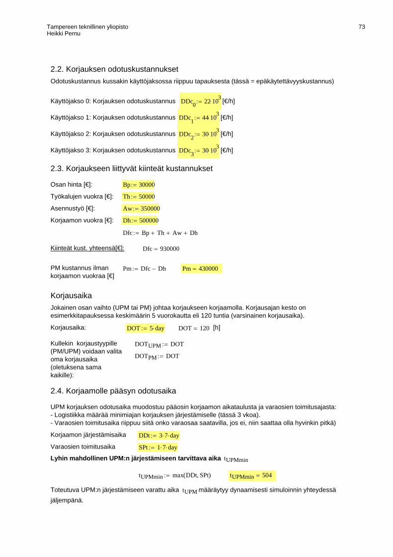
Tampereen teknillinen yliopistoHeikki Pernu
73
DOT 5 day⋅:= DOT 120= [h]
Kullekin korjaustyypille (PM/UPM) voidaan valita oma korjausaika (oletuksena sama kaikille):
DOTUPM DOT:=
DOTPM DOT:=
2.4. Korjaamolle pääsyn odotusaika
UPM korjauksen odotusaika muodostuu pääosin korjaamon aikataulusta ja varaosien toimitusajasta:- Logistiikka määrää minimiajan korjauksen järjestämiselle (tässä 3 vkoa).- Varaosien toimitusaika riippuu siitä onko varaosaa saatavilla, jos ei, niin saattaa olla hyvinkin pitkä)
Korjaamon järjestämisaika DDt 3 7⋅ day⋅:=
Varaosien toimitusaika SPt 1 7⋅ day⋅:=
Lyhin mahdollinen UPM:n järjestämiseen tarvittava aika tUPMmin
tUPMmin max DDt SPt,( ):= tUPMmin 504=
Toteutuva UPM:n järjestämiseen varattu aika tUPM määräytyy dynaamisesti simuloinnin yhteydessä jäljempänä.
2.2. Korjauksen odotuskustannuksetOdotuskustannus kussakin käyttöjaksossa riippuu tapauksesta (tässä = epäkäytettävyyskustannus)
Käyttöjakso 0: Korjauksen odotuskustannus DDc0 22 103⋅:= [€/h]
Käyttöjakso 1: Korjauksen odotuskustannus DDc1 44 103⋅:= [€/h]
Käyttöjakso 2: Korjauksen odotuskustannus DDc2 30 103⋅:= [€/h]
Käyttöjakso 3: Korjauksen odotuskustannus DDc3 30 103⋅:= [€/h]
2.3. Korjaukseen liittyvät kiinteät kustannukset
Osan hinta [€]: Bp 30000:=
Työkalujen vuokra [€]: Th 50000:=
Asennustyö [€]: Aw 350000:=
Korjaamon vuokra [€]: Dh 500000:=
Dfc Bp Th+ Aw+ Dh+:=
Kiinteät kust. yhteensä[€]: Dfc 930000=
PM kustannus ilman korjaamon vuokraa [€]
Pm Dfc Dh−:= Pm 430000=
KorjausaikaJokainen osan vaihto (UPM tai PM) johtaa korjaukseen korjaamolla. Korjausajan kesto on esimerkkitapauksessa keskimäärin 5 vuorokautta eli 120 tuntia (varsinainen korjausaika).
Korjausaika:
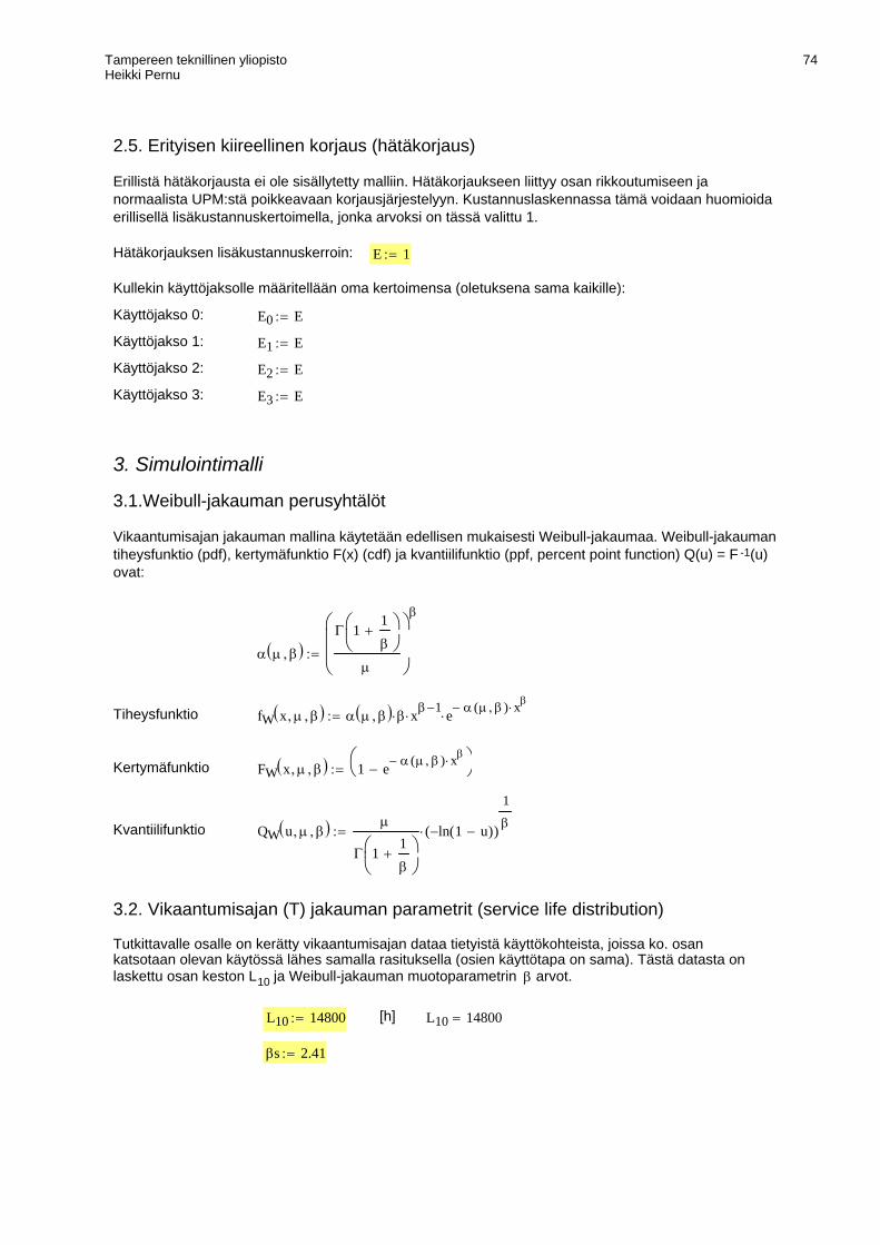
Tampereen teknillinen yliopistoHeikki Pernu
74
βs 2.41:=
L10 14800=[h]L10 14800:=
Tutkittavalle osalle on kerätty vikaantumisajan dataa tietyistä käyttökohteista, joissa ko. osan katsotaan olevan käytössä lähes samalla rasituksella (osien käyttötapa on sama). Tästä datasta on laskettu osan keston L10 ja Weibull-jakauman muotoparametrin β arvot.
3.2. Vikaantumisajan (T) jakauman parametrit (service life distribution)
QW u μ, β,( ) μ
Γ 11β
+⎛⎜⎝
⎞⎟⎠
ln 1 u−( )−( )
1
β⋅:=Kvantiilifunktio
FW x μ, β,( ) 1 e α μ β,( )− xβ⋅−
⎛⎝
⎞⎠:=Kertymäfunktio
fW x μ, β,( ) α μ β,( ) β⋅ xβ 1−⋅ e α μ β,( )− xβ⋅
⋅:=Tiheysfunktio
α μ β,( )Γ 1
1β
+⎛⎜⎝
⎞⎟⎠
μ
⎛⎜⎜⎝
⎞⎟⎟⎠
β
:=
Vikaantumisajan jakauman mallina käytetään edellisen mukaisesti Weibull-jakaumaa. Weibull-jakauman tiheysfunktio (pdf), kertymäfunktio F(x) (cdf) ja kvantiilifunktio (ppf, percent point function) Q(u) = F -1(u) ovat:
3.1.Weibull-jakauman perusyhtälöt
3. Simulointimalli
E3 E:=Käyttöjakso 3:
E2 E:=Käyttöjakso 2:
E1 E:=Käyttöjakso 1:
E0 E:=Käyttöjakso 0:
Kullekin käyttöjaksolle määritellään oma kertoimensa (oletuksena sama kaikille):
E 1:=Hätäkorjauksen lisäkustannuskerroin:
Erillistä hätäkorjausta ei ole sisällytetty malliin. Hätäkorjaukseen liittyy osan rikkoutumiseen ja normaalista UPM:stä poikkeavaan korjausjärjestelyyn. Kustannuslaskennassa tämä voidaan huomioida erillisellä lisäkustannuskertoimella, jonka arvoksi on tässä valittu 1.
2.5. Erityisen kiireellinen korjaus (hätäkorjaus)
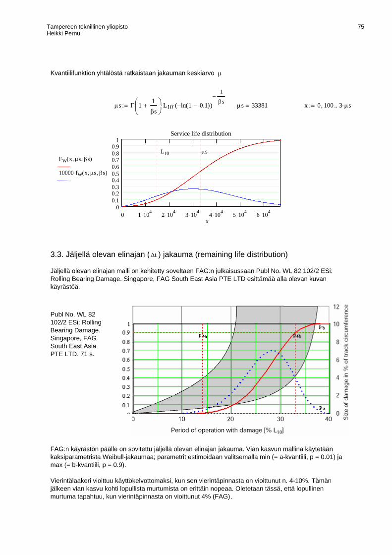
Tampereen teknillinen yliopistoHeikki Pernu
75
Kvantiilifunktion yhtälöstä ratkaistaan jakauman keskiarvo μ
μs Γ 11βs
+⎛⎜⎝
⎞⎟⎠
L10⋅ ln 1 0.1−( )−( )
1
βs−
⋅:= μs 33381= x 0 100, 3 μs⋅..:=
0 1 .104 2 .104 3 .104 4 .104 5 .104 6 .1040
0.10.20.30.40.50.60.70.80.9
1Service life distribution
FW x μs, βs,( )
10000 fW x μs, βs,( )⋅
μsL10
x
3.3. Jäljellä olevan elinajan (Δt ) jakauma (remaining life distribution)
Jäljellä olevan elinajan malli on kehitetty soveltaen FAG:n julkaisussaan Publ No. WL 82 102/2 ESi: Rolling Bearing Damage. Singapore, FAG South East Asia PTE LTD esittämää alla olevan kuvan käyrästöä.
Publ No. WL 82 102/2 ESi: Rolling Bearing Damage. Singapore, FAG South East Asia PTE LTD. 71 s.
FAG:n käyrästön päälle on sovitettu jäljellä olevan elinajan jakauma. Vian kasvun mallina käytetään kaksiparametrista Weibull-jakaumaa; parametrit estimoidaan valitsemalla min (= a-kvantiili, p = 0.01) ja max (= b-kvantiili, p = 0.9).
Vierintälaakeri vioittuu käyttökelvottomaksi, kun sen vierintäpinnasta on vioittunut n. 4-10%. Tämän jälkeen vian kasvu kohti lopullista murtumista on erittäin nopeaa. Oletetaan tässä, että lopullinen murtuma tapahtuu, kun vierintäpinnasta on vioittunut 4% (FAG) .
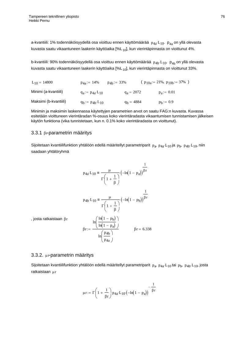
Tampereen teknillinen yliopistoHeikki Pernu
76
μr Γ 11βr
+⎛⎜⎝
⎞⎟⎠
p4a⋅ L10⋅ ln 1 pa−( )−( )1
βr−
⋅:=
Sijoitetaan kvantiilifunktion yhtälöön edellä määritellyt parametriparit pa, p4a L10⋅ tai pb, p4b L10⋅ , josta
ratkaistaan μr
3.3.2. μr-parametrin määritys
βr 6.338=βr
lnln 1 pb−( )ln 1 pa−( )
⎛⎜⎝
⎞⎟⎠
lnp4b
p4a
⎛⎜⎝
⎞⎟⎠
:=
, josta ratkaistaan βr
p4b L10⋅μ
Γ 11β
+⎛⎜⎝
⎞⎟⎠
ln 1 pb−( )−( )1
βr⋅=
p4a L10⋅μ
Γ 11β
+⎛⎜⎝
⎞⎟⎠
ln 1 pa−( )−( )1
βr⋅=
Sijoitetaan kvantiilifunktion yhtälöön edellä määritellyt parametriparit pa, p4a L10⋅ ja pb, p4b L10⋅ , niin saadaan yhtälöryhmä
3.3.1 βr-parametrin määritys
Minimin ja maksimin laskennassa käytettyjen parametrien arvot on saatu FAG:n kuvasta. Kuvassa esitetään vioittuneen vierintäradan %-osuus koko vierintäradasta vikaantumisen tunnistamisen jälkeisen käytön funktiona (vika tunnistetaan, kun n. 0.1% koko vierintäradasta on vioittunut).
pb 0.9:=qb 4884=qb p4b L10⋅:=Maksimi (b-kvantiili)
pa 0.01:=qa 2072=qa p4a L10⋅:=Minimi (a-kvantiili)
( p10a 21%:= , p10b 37%:= )p4b 33%:=p4a 14%:=L10 14800=
b-kvantiili: 90% todennäköisyydellä osa vioittuu ennen käyttömäärää p4b L10⋅ . p4b on yllä olevasta kuvasta saatu vikaantuneen laakerin käyttöaika [%L10], kun vierintäpinnasta on vioittunut 33%.
a-kvantiili: 1% todennäköisyydellä osa vioittuu ennen käyttömäärää p4a L10⋅ . p4a on yllä olevasta kuvasta saatu vikaantuneen laakerin käyttöaika [%L10], kun vierintäpinnasta on vioittunut 4%.

Tampereen teknillinen yliopistoHeikki Pernu
77
FkW x( ) FW x μr, βr,( ):= fkW x( ) fW x μr, βr,( ):= QkW u( ) QW u μr, βr,( ):=
Aika-akselina kalenteriaika: F1Wk x( ) FW
xK
μs, βs,⎛⎜⎝
⎞⎟⎠
:= FkWk x( ) FWxK
μr, βr,⎛⎜⎝
⎞⎟⎠
:= fkWk x( )1K
fWxK
μr, βr,⎛⎜⎝
⎞⎟⎠
⋅:=
4.1. Valitaan huoltoväli H ja huoltomarginaali ΔH:
H: H205
year⋅:=
ΔH: ΔH 0.1 year⋅:=
Huoltoväliä ja huoltomarginaalia varioimalla voidaan etsiä minimikustannukset (tässä ei ole automaattista minimin etsintää).
UPM:n vaatima minimiaika (aikaväli vian havaitsemisesta korjauksen aloitukseen)
tUPMmin: tUPMmin 504=
Todennäköisyys, että vian havaitsemisen jälkeen aikavälillä 0... tUPMmin 504= osa särkyy on FkWk tUPMmin( ) 0.00000009889= .
L10 14800= μr 3984=
p4a 14 %= p4a L10⋅ 2072=
p4b 33 %= p4b L10⋅ 4884= p 0 0.01, 0.4..:= u 0 1..:=
0 0.05 0.1 0.15 0.2 0.25 0.3 0.35 0.40
0.10.20.30.40.50.60.70.80.9
1Size of damage distribution
pa
pb
FW L10 p⋅ μr, βr,( )
p4a p4b
p
4. Satunnaisten vikojen ja huoltojen yhdistetty simulointi
μs 33381= βs 2.41= F1W x( ) FW x μs, βs,( ):=
μr 3984= βr 6.3=
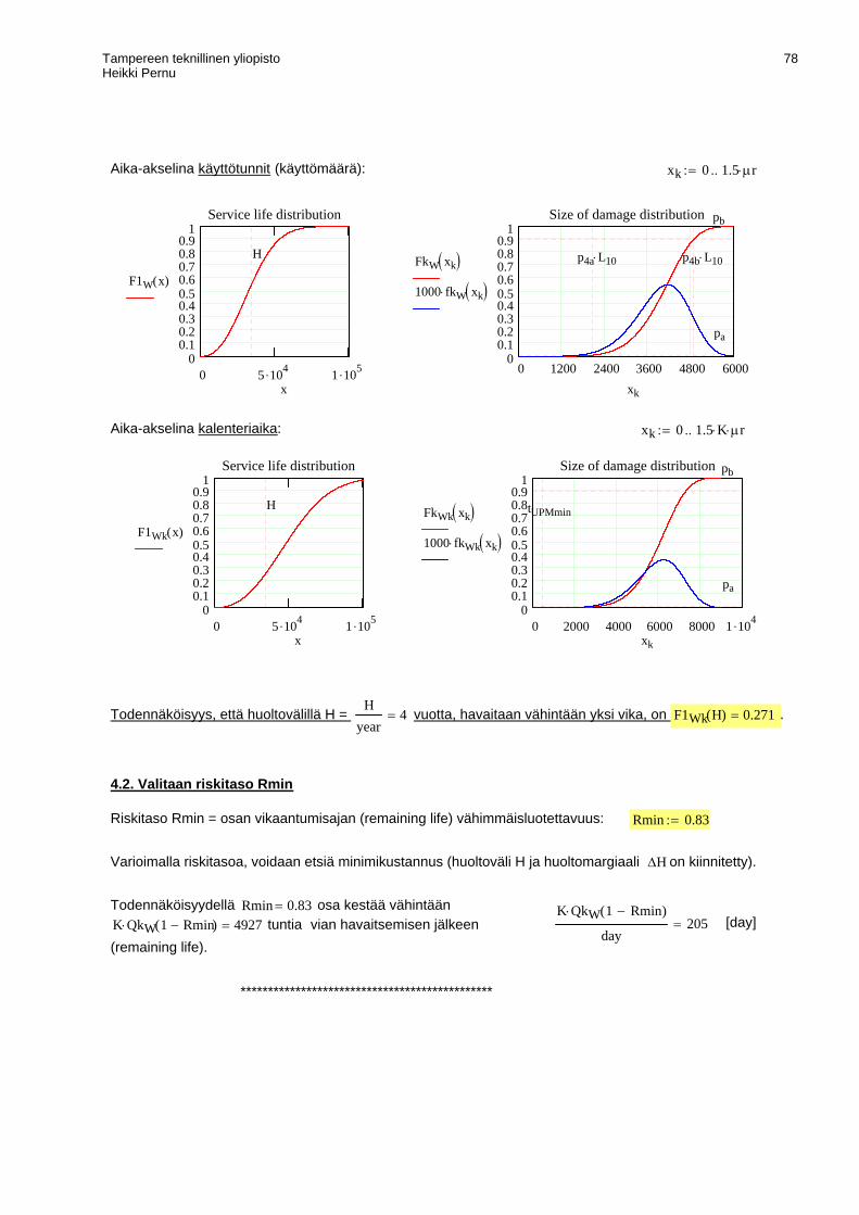
Tampereen teknillinen yliopistoHeikki Pernu
78
**********************************************
[day]K QkW 1 Rmin−( )⋅
day205=
Todennäköisyydellä Rmin 0.83= osa kestää vähintään K QkW 1 Rmin−( )⋅ 4927= tuntia vian havaitsemisen jälkeen (remaining life).
Varioimalla riskitasoa, voidaan etsiä minimikustannus (huoltoväli H ja huoltomargiaali ΔH on kiinnitetty).
Rmin 0.83:=Riskitaso Rmin = osan vikaantumisajan (remaining life) vähimmäisluotettavuus:
4.2. Valitaan riskitaso Rmin
Todennäköisyys, että huoltovälillä H = H
year4= vuotta, havaitaan vähintään yksi vika, on F1Wk H( ) 0.271= .
0 2000 4000 6000 8000 1 .1040
0.10.20.30.40.50.60.70.80.9
1Size of damage distribution
pa
pb
FkWk xk( )1000 fkWk xk( )⋅
tUPMmin
xk0 5 .104 1 .105
00.10.20.30.40.50.60.70.80.9
1Service life distribution
F1Wk x( )
H
x
xk 0 1.5 K⋅ μr⋅..:=Aika-akselina kalenteriaika:
0 1200 2400 3600 4800 60000
0.10.20.30.40.50.60.70.80.9
1Size of damage distribution
pa
pb
FkW xk( )1000 fkW xk( )⋅
p4a L10⋅ p4b L10⋅
xk0 5 .104 1 .105
00.10.20.30.40.50.60.70.80.9
1Service life distribution
F1W x( )
H
x
xk 0 1.5 μr⋅..:=Aika-akselina käyttötunnit (käyttömäärä):
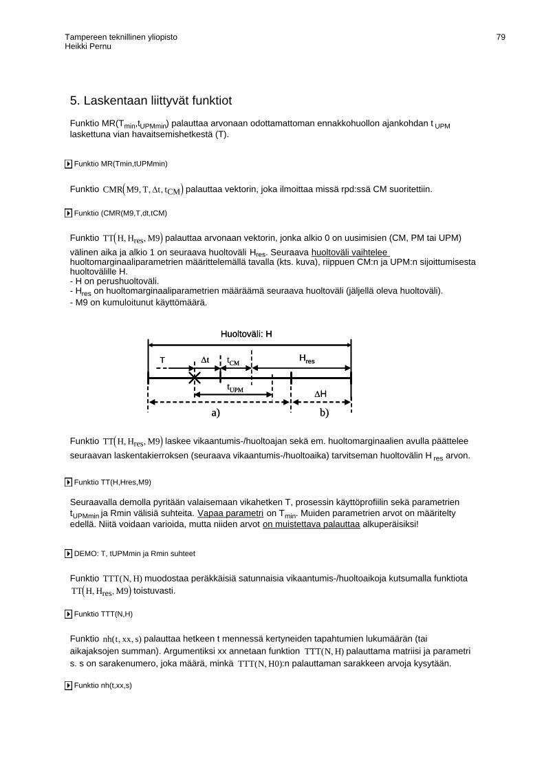
Tampereen teknillinen yliopistoHeikki Pernu
79
Funktio nh(t,xx,s)
Funktio nh t xx, s,( ) palauttaa hetkeen t mennessä kertyneiden tapahtumien lukumäärän (tai aikajaksojen summan). Argumentiksi xx annetaan funktion TTT N H,( ) palauttama matriisi ja parametri s. s on sarakenumero, joka määrä, minkä TTT N H0,( ):n palauttaman sarakkeen arvoja kysytään.
Funktio TTT(N,H)
Funktio TTT N H,( ) muodostaa peräkkäisiä satunnaisia vikaantumis-/huoltoaikoja kutsumalla funktiota TT H Hres, M9,( ) toistuvasti.
DEMO: T, tUPMmin ja Rmin suhteet
Seuraavalla demolla pyritään valaisemaan vikahetken T, prosessin käyttöprofiilin sekä parametrien tUPMmin ja Rmin välisiä suhteita. Vapaa parametri on Tmin. Muiden parametrien arvot on määritelty edellä. Niitä voidaan varioida, mutta niiden arvot on muistettava palauttaa alkuperäisiksi!
Funktio TT(H,Hres,M9)
Funktio TT H Hres, M9,( ) laskee vikaantumis-/huoltoajan sekä em. huoltomarginaalien avulla päättelee seuraavan laskentakierroksen (seuraava vikaantumis-/huoltoaika) tarvitseman huoltovälin H res arvon.
a) b)
ΔH
Δt
tUPM
T tCM
Huoltoväli: H
Hres
a) b)
ΔH
Δt
tUPM
T tCM
Huoltoväli: H
Hres
Funktio TT H Hres, M9,( ) palauttaa arvonaan vektorin, jonka alkio 0 on uusimisien (CM, PM tai UPM) välinen aika ja alkio 1 on seuraava huoltoväli Hres. Seuraava huoltoväli vaihtelee huoltomarginaaliparametrien määrittelemällä tavalla (kts. kuva), riippuen CM:n ja UPM:n sijoittumisesta huoltovälille H.- H on perushuoltoväli.- Hres on huoltomarginaaliparametrien määräämä seuraava huoltoväli (jäljellä oleva huoltoväli).- M9 on kumuloitunut käyttömäärä.
Funktio (CMR(M9,T,dt,tCM)
Funktio CMR M9 T, Δt, tCM,( ) palauttaa vektorin, joka ilmoittaa missä rpd:ssä CM suoritettiin.
Funktio MR(Tmin,tUPMmin)
Funktio MR(Tmin,tUPMmin) palauttaa arvonaan odottamattoman ennakkohuollon ajankohdan t UPM laskettuna vian havaitsemishetkestä (T).
5. Laskentaan liittyvät funktiot

Tampereen teknillinen yliopistoHeikki Pernu
80
PM: ΛPM t( ) ΛPM0 t( ) ΛPM1 t( )+ ΛPM2 t( )+ ΛPM3 t( )+ ΛPM4 t( )+:=ΛPM T( ) =
Odottamattomien huoltojen (UPM) lkm.
Odottamattomat huollot (UPM) yhteensä:
UPM: ΛUPM t( )1M
0
M 1−
i
nh t nti, 12,( )∑=
⋅:=ΛUPM T( ) 0.9673=
Huoltoja yhteensä (PM + UPM):
UPM + PM: ΛRen t( ) ΛUPM t( ) ΛPM t( )+:= ΛRen T( ) 4.967=
Särkymisien lkm. yhteensä (alue a + b):
CM (alue a + b): ΛCM t( ) ΛCMa t( ) ΛCMbr t( ) ΛCMbt t( )+( )+:= ΛCM T( ) 0.0311=
6. Tapahtumien simulointi
Simuloidaan M kpl TTT N H,( ) -otoksia.
Uusimisien lukumäärä: N 12:=
Koska etukäteen ei tiedetä, kuinka monta uusimista tulee tapahtumaan tarkastelujakson T aikana, on N:n arvo valittava riittävän suureksi tai on haettava kokeilemalla sellainen arvo, että laskenta menee läpi. (Jos yhdessäkin otoksessa on liian vähän uusimisia, ts. korjaus-vika-korjaus -prosessin kesto on < T, niin laskenta ei mene läpi!
Huoltoväli (4.1): H 35040= H 4 year=
Otosten lukumäärä: M 10000:= i 0 M 1−..:= nti TTT N H,( ):=
********************************************
Tarkastelujakso (kalenteriaikaa): T 19.99 year⋅:= T =
Suunniteltujen huoltojen (PM) lkm.
Suunnitellut huollot (PM) yhteensä:

Tampereen teknillinen yliopistoHeikki Pernu
81
DDb1 t( )1
M ΛCMb1 t( )⋅ 10 15−+ 0
M 1−
i
nh t nti, 30,( )∑=
⋅:= DDb1 T( ) 0=
CM (rpd2) (alue a/b, tUPM>H): DDb2 t( )1
M ΛCMb2 t( )⋅ 10 15−+ 0
M 1−
i
nh t nti, 31,( )∑=
⋅:= DDb2 T( ) 504=
CM (rpd3) (alue a/b, tUPM>H): DDb3 t( )1
M ΛCMb3 t( )⋅ 10 15−+ 0
M 1−
i
nh t nti, 32,( )∑=
⋅:= DDb3 T( ) 504=
Odotusajat alueella b:
Suuri riskiDD0b t( )
1
M ΛPM4 t( )⋅ 10 10−+ 0
M 1−
i
nh t nti, 24,( )∑=
⋅:=PM (alue b, riski): DD0b T( ) 0=
DD4b t( )1
M ΛCMbr t( )⋅ 10 10−+ 0
M 1−
i
nh t nti, 28,( )∑=
⋅:=CM (alue b, riski): DD4b T( ) 0=
Normaali riski
DD1b t( )1
M ΛPM3 t( )⋅ 10 10−+ 0
M 1−
i
nh t nti, 25,( )∑=
⋅:=PM (alue b, tUPM>H): DD1b T( ) 225=
Keskimääräinen odotusaika CM:ää kohti [h] (HUOM. odotusaika sijoittuu pääsääntöisesti edelliseen sektoriin)7. Huoltojen odotusajat
Odotusajat kussakin rpd sektorissa (alue a):
CM (a; rpd0): DDa0 t( )1
M ΛCMa0 t( )⋅ 10 10−+ 0
M 1−
i
nh t nti, 33,( )∑=
⋅:= DDa0 T( ) 187.15=
CM (a; rpd1): DDa1 t( )1
M ΛCMa1 t( )⋅ 10 10−+ 0
M 1−
i
nh t nti, 34,( )∑=
⋅:= DDa1 T( ) 504=
CM (a; rpd2): DDa2 t( )1
M ΛCMa2 t( )⋅ 10 10−+ 0
M 1−
i
nh t nti, 35,( )∑=
⋅:= DDa2 T( ) 245.75=
CM (a; rpd3):DDa3 t( )
1
M ΛCMa3 t( )⋅ 10 10−+ 0
M 1−
i
nh t nti, 36,( )∑=
⋅:= DDa3 T( ) 504=
Odotusajat kussakin käyttöjaksossa (alue a/b):
CM (rpd0) (alue a/b, tUPM>H): DDb0 t( )1
M ΛCMb0 t( )⋅ 10 15−+ 0
M 1−
i
nh t nti, 29,( )∑=
⋅:= DDb0 T( ) 0=
CM (rpd1) (alue a/b, tUPM>H):

Tampereen teknillinen yliopistoHeikki Pernu
82
************************************************************************
CORen T( ) 4550735.8=CORen t( ) COUPM t( ) CODD t( )+ COCM t( )+:=
Kustannukset yhteensä (UPM:t + korjaamoviiveet + CM:t):
**********************
CODD T( ) 379584=CODD t( ) COCMDa t( ) COCMDab t( )+ COPM3 t( )+ COPM4 t( )+ COCMbr t( )+:=
Korjaamoviivekustannukset yhteensä:
Kustannus = Lukumäärä * (menetetty)myyntitulo * keskimääräinen odotusaikaOdotusaika sattuu pääsääntöisesti UPM:ää edeltävään käyttöjaksoon (voi periaatteessa olla niin pitkä, että koskettaa kahta tai useampaa sektoria (joilla on eri kustannus) samanaikaisesti, mutta sitä ei tässä huomioida.
8.3. Korjaamoviivekustannukset
COCM T( ) 148635=COCM t( ) CMCOa t( ) CMCOb T( )+ CMCObr T( )+:=
CM kustannukset yhteensä
8.2. Satunnaiset viat (CM)
COUPM T( ) 4.02 106×=COUPM t( ) COUPM0 t( ) COUPM1 t( )+ COUPM2 t( )+ COUPM3 t( )+:=
UPM kustannukset yhteensä:
8.1. Odottamattomat huollot (UPM)
T 19.99 year=Korjaamoaika: DOTUPM 120= [h]Kiinteät kustannukset yhteensä.: Dfc 930000= €
Korjaamoon liittyvät kiinteät kustannukset muodostuvat seuraavista osista: Laakerikustannus, työkalujen vuokra, asennustyö ja korjaamovuokra.
Kustannus = odotusaika*(menetetty)myyntitulo + korjaamoaika*(menetetty)revenu + kiinteä kustannus
Kustannukset kaikille vika- ja korjaustyypeille ( € ).
8. Kustannuslaskenta

KOTEL 256
Total number of pages in Appendix 61
APPENDIX 4
CASE-STUDIES: COMPANIES PRESENTATIONS

BRED‐projektiin osallistuvien yrityksien esityksiä case‐projekteista
‐ Kone ‐ Wärtsilä ‐ CarcoMacGregor

KONE BRED projects External summary
© 2009 KONE Corporation BRED External (LAB-01.89.014) All rights reserved. Page 2 of 18 (-) 2009-03-16
Table of contents 1 PURPOSE OF THIS DOCUMENT ..................................................................................................... 3 2 SCOPE .............................................................................................................................................. 4 3 DEFINITIONS .................................................................................................................................... 4 4 GENERAL .......................................................................................................................................... 5
4.1 Background .............................................................................................................................. 7 4.2 Goals of the Projects ................................................................................................................ 8
5 PROJECT CASES ............................................................................................................................. 8 5.1 Product Dependability Follow-up based on Field Data ............................................................. 8 5.2 Call out rate target setting and feasibility check improvement ................................................ 10
5.2.1 Field Data Allocation for existing Call Out Rate data ............................................... 10 5.2.2 Specification and allocation of InnoTrack’s availability and maintenance cost requirements .......................................................................................................................... 12
5.3 KONE Product’s Quality and Reliability metrics harmonization .............................................. 16 5.4 Customer Value-Driven Design for Reliability in Product Development .................................. 16
6 VERSION HISTORY ........................................................................................................................ 18
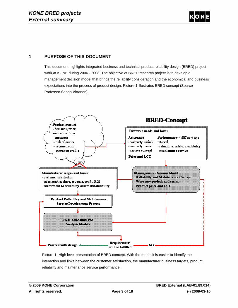
KONE BRED projects External summary
© 2009 KONE Corporation BRED External (LAB-01.89.014) All rights reserved. Page 3 of 18 (-) 2009-03-16
1 PURPOSE OF THIS DOCUMENT
This document highlights integrated business and technical product reliability design (BRED) project
work at KONE during 2006 - 2008. The objective of BRED research project is to develop a
management decision model that brings the reliability consideration and the economical and business
expectations into the process of product design. Picture 1 illustrates BRED concept (Source
Professor Seppo Virtanen).
Picture 1. High level presentation of BRED concept. With the model it is easier to identify the
interaction and links between the customer satisfaction, the manufacturer business targets, product
reliability and maintenance service performance.

KONE BRED projects External summary
© 2009 KONE Corporation BRED External (LAB-01.89.014) All rights reserved. Page 4 of 18 (-) 2009-03-16
2 SCOPE
This document describes the core activities relating to KONE BRED projects done by the Service
Development and Reliability Laboratory departments. However this document does not cover in detail
findings and results of work carried out as there is a need for external communication. More detailed
documentation is available for KONE purposes.
The scope of KONE Projects was to improve maintainability and reliability engineering capabilities
towards customer value driven and total quality management directions. Scope included Service
Equipment Business related reliability metrics as Call Out Rate and availability. In addition pricing and
risk analysis of maintenance contracts were drafted during project. Warranty target setting for New
Equipment Business was excluded from the scope. However methods and structure suits well for
warranty data management as well.
High data quality plays an important role in data management when data is turned into information
and further to fact based decisions. Two Master’s Thesis were carried out. Improvement actions
relating to field data collection were the part of a BRED-project related Master’s Thesis (Product
dependability follow-up based on field data). A second MSc. thesis was conducted concerning the
translation of customers’ perceptions into product reliability requirements. This thesis is not an actual
part of the BRED-project, but however it has a strong connection to its topics and therefore briefly
presented in this document.
Other projects and activities were based on existing theories relating to failure logic analyzing and
allocation of reliability requirements. Thus main effort of the project is put into the development of
applications, documentation, implementation and training.
3 DEFINITIONS
COR Call Out Rate DFR Design for Reliability FTA Fault Tree Analysis KTO KONE Technology Organization LCC Life Cycle Cost NEB New equipment Business TCO Total Cost of Ownership PCM Product Change Management PD Project Product Development Project PDM Product Development Matrix
KONE BRED projects External summary
© 2009 KONE Corporation BRED External (LAB-01.89.014) All rights reserved. Page 5 of 18 (-) 2009-03-16
RCM Reliability Centered Maintenance ROI Return on Investment SEB Service Equipment Business
4 GENERAL
KONE delivers a performance edge to it’s customers by creating the best user experience with
innovative people flow solutions. High quality People Flow Solutions enable people to move smoothly,
safely, comfortably and efficiently during whole life cycle. Reliable products maximize the
performance of buildings of customers. Thus KONE has committed towards continuous quality
improvement.
Elevator system is architecture of 12 subsystems achieving specified performance. In addition to
customer-based performance requirements elevator system needs to meet its environmental
(sustainability), safety and quality requirements. Quality of an elevator has great impact to customer
satisfaction. As reliability is time-oriented aspect of quality its requirements are targeted in calendar
time or usage rate. Not only customer satisfaction but also business profitability can be secured when
reliability targets are well considered.
Elevator design work follows concurrent product development model and there are several key
factors to deal and trade off. These factors include performance (speed, nominal load), features
(machine-roomless), material cost, time to market and reliability. Design team needs to emphasize
these factors optimally so that successful products can be launched into the market. Trade offing and
finding correct “recipe” is very important when company is providing maintenance services and
service repairs. Life cycle cost approach help finding correct balance between multiple design needs.
Without commonly agreed terminology and decision making models personal opinions may have too
strong influence. In addition correct time and timing are important. The beginning of the product
development is the right moment to raise LCC issues because critical design decisions are made
then. It is not very fruitful to raise and communicate LCC if design is relative mature. Reliability has
important role in LCC and in total cost of ownership (TCO) when service business is on landscape.
Reliability Centered Maintenance RCM is commonly known approach in industries having high need
for safety and profitability based on operational performance. Therefore reliability related targets must
be well considered and agreed during early phase of product development.
Reliability definition includes three important aspects, probability of operating without failure within
given time under certain conditions. E.g. It can be allowed that system may have one technical failure
annually (with low severity) during its 15 years useful life period under typical residential use. As it can
be seen reliability target setting includes top management level strategic issues and thus top
KONE BRED projects External summary
© 2009 KONE Corporation BRED External (LAB-01.89.014) All rights reserved. Page 6 of 18 (-) 2009-03-16
management is the correct forum to decide reliability targets for an elevator, escalator or any other
system.
Service business profitability, sustainability, global competition and continues need to improve
customer satisfaction are the drivers for quality improvement. System level targets are normally set
based on the understanding the current level of reliability and philosophy of continuous improvement
is used. This is valid especially in design projects, which are using existing design solutions and only
some part of new equipment is re-designed. However making continuous improvement with linear
approach has major gaps in case of revolutionary product development projects providing People
Flow solutions as benchmark data does not exist. In order to support target setting discussions and
decision every business needs good methods and tools for LCC and TCO evaluations. How top
management can set reliability targets then? In addition to customer value and competitors offering
acceptable level of cost of unreliability must be understood. This acceptable level depends on many
factors including service contract pricing originating based on market condition.
KONE BRED cases created, communicated and implemented will support well further development
and implementation of more complex methods towards better estimation of KONE TCO.

KONE BRED projects External summary
© 2009 KONE Corporation BRED External (LAB-01.89.014) All rights reserved. Page 7 of 18 (-) 2009-03-16
4.1 Background
Reliability Laboratory is responsible for KONE Way’s Solution Creation process’s improve quality and
reliability activities, see picture 2.
Picture 2. KONE Way includes three core processes supported with management processes. KONE Technology Organization KTO is responsible for the solution creation process and it includes five sub processes. KTO Quality and Reliability including the Reliability Laboratory is the organization driving continuous quality and reliability improvements. Reliability Laboratory’s mission is to ensure product reliability and quality throughout the life cycle of the product.
The main idea of Design for Reliability DFR is to improve and ensure that design meets its reliability
goals without extensive over designing leading to increase of material costs. DFR also shortens time
to market as it includes tools allowing part of the verification work to be carried out during early stages
of product development and this minimizes risk for time and effort consuming test-fix-test cycles.
Service Development is part of Concurrent Engineering and supports PD project to make sure
product is easy to maintain and fulfilling service business needs.
When system level targets are specified and allocated to component level then Product Development
projects with the help of “Service Development” and “KTO Quality and Reliability” are able to calculate
Return of Investment based on LCC and Reliability Centered Maintenance approach.
KONE BRED projects External summary
© 2009 KONE Corporation BRED External (LAB-01.89.014) All rights reserved. Page 8 of 18 (-) 2009-03-16
4.2 Goals of the BRED Projects
KONE BRED project and activities done besides have following goals:
1. Harmonize the quality and reliability metric terminology within KONE
2. Collect, investigate and utilize existing up-to date Call Out Rate COR data more efficiently
3. Data utilization and improve present capabilities to distribute and communicate reliability figures
during early PD project phases.
4. LCC and PD Project target setting related people communication, process and tool development
and improvements.
5. Study Fault tree based method to support Maintenance Need Analysis and Design FMEA etc
tools.
5 PROJECT CASES
Following three BRED projects and one Master thesis having link to BRED project goals are briefly
summarized in following sections.
5.1 Product Dependability Follow-up based on Field Data
The first KONE BRED project case was a Master‘s Thesis that examined products’ perceived
dependability follow-up and reliability centred maintenance planning. Thesis was performed in the
Service Development department with strong co-operation with the Reliability Laboratory.
The basic purpose of the thesis was to examine the dependability of the products that are already in
field. The objects of interests were failures as well as performed repair and maintenance actions.
Plenty of field data has been saved into the management and maintenance systems of KONE. The
evaluation of the current field data and possibility to utilise the data in maintenance planning and DFR
were researched.
The aim of the thesis was divided into five main stages:
1. Locate field data sources and analyse current data
2. Find a method to model the lifetime of component based on the field data
3. Optimise a maintenance strategy for a critical component
4. Identify opportunities to improve products’ dependability follow-up process
5. Gather up opportunities for product reliability and availability growth
KONE BRED projects External summary
© 2009 KONE Corporation BRED External (LAB-01.89.014) All rights reserved. Page 9 of 18 (-) 2009-03-16
A starting point for a follow-up was the back reported field data from maintenance actions, which
included for example the reason and target of the work as well as the performed actions on site. The
current level of field data was evaluated and methods to extract data were examined. The material for
this study was collected from four frontline units, starting from year 2003. At the beginning, the
extracted field data was analysed in general level. In addition, comparisons between countries were
performed to understand the content and reliability of data.
The major part of the thesis consisted of a dependability case study that was done for a elevator
component. The performed field data analyses have identified that the particular component failure is
one of the most frequently reported call-out root cause in MonoSpace elevators. KONE aims to
minimize call-outs by performing appropriate maintenance, which is an important financial issue, and
increases customer satisfaction. In the first phase of the case study, a reliability function was
modelled for the component. The Kaplan-Meier estimation method was utilised for modelling. The
used calculation formulas were developed by cooperating with the reliability engineering experts of
Tampere University of Technology. After that, the cost factors of corrective and preventive
maintenance were evaluated for the component. Then, by utilising the modeled reliability function and
ELMAS and RAMoptim software the most suitable maintenance strategy was optimised. To
understand cost factors, the dependability simulation was performed for different time scenarios as
typical customer warranty period, a typical maintenance contract period and whole elevator’s lifetime.
In the second phase of the case study a fault tree analysis was performed. The aim was to simulate
the root causes of the component’s failures. The fault tree model was tested and it was found to be
functional in failure analysis. A similar fault tree model could also be used in product design phase. It
provides a possibility to compare the effects of different parts on the dependability of the designed
product, as is shown in InnoTrack BRED-case.
Thesis’ conclusions outlined demands and advantages for more systematic dependability follow-up
process. The main demands include the further development of back reporting procedures and follow-
up tools. In this way maintenance processes can be developed. Since the beginning of the BRED-
project KONE has taken a great step forward around this topic. Possibilities to improve product
dependability can be achieved by increasing the number of preventive component replacements and
the further development of remote monitoring utilization. The experiences collected from the methods
of the thesis and the reliability software used in preventive maintenance optimization and DFR were
promising.
The more detailed results of the case study of this MSc. thesis were published globally by Springer in
“Proceedings of the 3rd World Congress on Engineering Asset Management and Intelligent
Maintenance Systems Conference (WCEAM-IMS 2008)”.

KONE BRED projects External summary
© 2009 KONE Corporation BRED External (LAB-01.89.014) All rights reserved. Page 10 of 18 (-) 2009-03-16
5.2 Call out rate target setting and feasibility check improvement
The Fault Tree Analyze FTA based model was applied in a benefit of improving existing methods to
specify and allocate system level reliability requirements. Modeling and allocation was done for two
cases, existing MonoSpace COR and for a new innovation. The results of applications developed can
be used to as an input for quality improvement based project start-ups.
Application is based on the statistical customer focused TOP-DOWN approach. The main benefit of
top-down approach is that it can be adopted with the present level of data and when more in detail
data is available accuracy of the analysis can be improved. These will point out potential components
for cost efficient call out reduction without forgetting failure effects noticed by the final users (customer
value).
5.2.1 Field Data Allocation for existing Call Out Rate data
First COR target setting and feasibility check improvement case was tried with elevator doors
because of available technical understanding about root causes in addition to high quality COR data
originating from product dependability follow-up based on field data Master’s Thesis. Then developed
model and application was applied to cover whole existing MonoSpace.
The primary purpose of the elevator doors is guarantee passenger safety both inside car and at the
landings. Car door and landing doors are usually separated when reliability analysis are done as
there is only one car door in a single elevator. The number of landing doors depends on the number
of landings elevator is serving. In addition landing door subsystem is fairly simple when compared to
car door as there are no electronic components and all electrical components are fairly simple. As
one elevator system has several doors elevator system reliability will suffer if each doors have design
related defects that cannot be corrected easily in field conditions.
An operation of elevator door system is one of the most important factors for customer satisfaction. If
doors are not closing properly whole elevator system is not able to operate. Also “soft failures” like
noise and vibration are causing easily customer dissatisfaction and further unscheduled site visits and
cost for KONE service business. Therefore designing of any door related systems of components
must fulfill tight reliability requirements nothing to speak about safety functions of the doors.
Call out rate for the door was calculated by dividing number of annual site visits with the number of
lifts in service. Data includes several root causes and some with no relationship to design quality non-
parametric calculation method was used and assumption was made that failure rate is constant
(exponentially distributed). Allocation included following five logical levels.
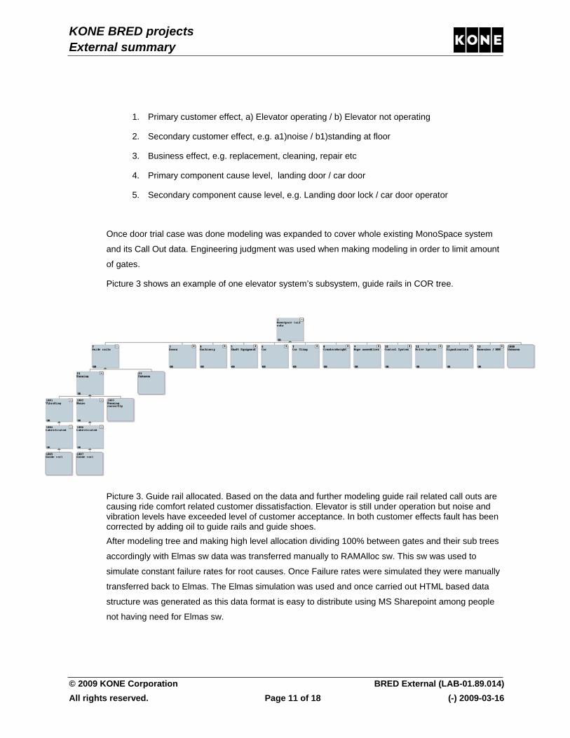
KONE BRED projects External summary
© 2009 KONE Corporation BRED External (LAB-01.89.014) All rights reserved. Page 11 of 18 (-) 2009-03-16
1. Primary customer effect, a) Elevator operating / b) Elevator not operating
2. Secondary customer effect, e.g. a1)noise / b1)standing at floor
3. Business effect, e.g. replacement, cleaning, repair etc
4. Primary component cause level, landing door / car door
5. Secondary component cause level, e.g. Landing door lock / car door operator
Once door trial case was done modeling was expanded to cover whole existing MonoSpace system
and its Call Out data. Engineering judgment was used when making modeling in order to limit amount
of gates.
Picture 3 shows an example of one elevator system’s subsystem, guide rails in COR tree.
Picture 3. Guide rail allocated. Based on the data and further modeling guide rail related call outs are causing ride comfort related customer dissatisfaction. Elevator is still under operation but noise and vibration levels have exceeded level of customer acceptance. In both customer effects fault has been corrected by adding oil to guide rails and guide shoes. After modeling tree and making high level allocation dividing 100% between gates and their sub trees
accordingly with Elmas sw data was transferred manually to RAMAlloc sw. This sw was used to
simulate constant failure rates for root causes. Once Failure rates were simulated they were manually
transferred back to Elmas. The Elmas simulation was used and once carried out HTML based data
structure was generated as this data format is easy to distribute using MS Sharepoint among people
not having need for Elmas sw.
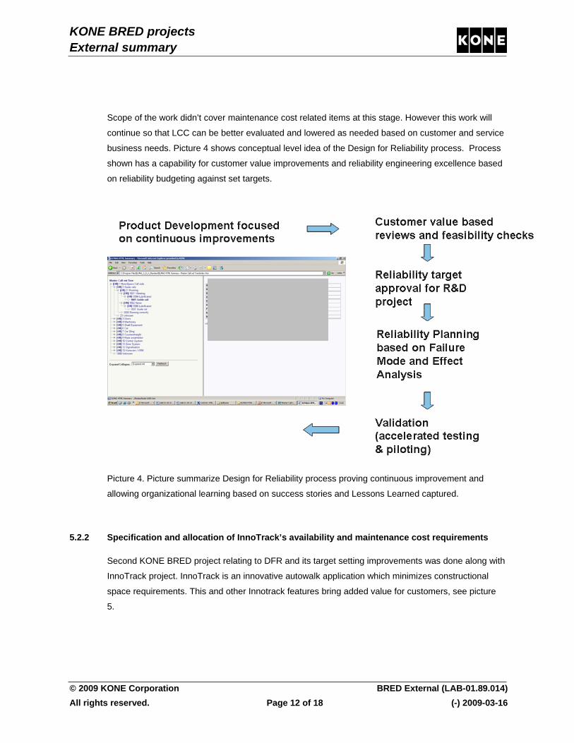
KONE BRED projects External summary
© 2009 KONE Corporation BRED External (LAB-01.89.014) All rights reserved. Page 12 of 18 (-) 2009-03-16
Scope of the work didn’t cover maintenance cost related items at this stage. However this work will
continue so that LCC can be better evaluated and lowered as needed based on customer and service
business needs. Picture 4 shows conceptual level idea of the Design for Reliability process. Process
shown has a capability for customer value improvements and reliability engineering excellence based
on reliability budgeting against set targets.
Picture 4. Picture summarize Design for Reliability process proving continuous improvement and
allowing organizational learning based on success stories and Lessons Learned captured.
5.2.2 Specification and allocation of InnoTrack’s availability and maintenance cost requirements
Second KONE BRED project relating to DFR and its target setting improvements was done along with
InnoTrack project. InnoTrack is an innovative autowalk application which minimizes constructional
space requirements. This and other Innotrack features bring added value for customers, see picture
5.

KONE BRED projects External summary
© 2009 KONE Corporation BRED External (LAB-01.89.014) All rights reserved. Page 13 of 18 (-) 2009-03-16
Picture 5. Picture highlights customer value that InnoTrack provides compared to existing solutions.
These were the key characteristic concerning Total Cost of Ownership in InnoTrack case:
Reliability and Availability
Life cycle cost: Based on installed equipment, maintenance cost, spare parts, energy
consumption over a period of 20 years
Maintenance intervals
Preventive replacement of different parts
Spare part list and prices
In order to make PD Project’s work easier modeling and system level allocation was done based on
availability, COR requirements and service business monetary requirements. Picture 6 illustrates high
level allocation.

KONE BRED projects External summary
© 2009 KONE Corporation BRED External (LAB-01.89.014) All rights reserved. Page 14 of 18 (-) 2009-03-16
Picture 6. Targeted availability and maintenance costs were allocated using to gates, scheduled site
visits and Call outs. Modeling was done till appropriate design level.
The primary purpose of this case was to divide customer based system level availability requirement
to subsystem and further to key component level. This information is used for reliability verification
purposes including reliability related discussions with suppliers. Allocation provides also good input
for further Reliability Centered Maintenance studies (optimization of maintenance).
As quantitative field data is not available and design is at its early stages many engineering
judgments are done supported with formulas shown in the picture 7. Both Elmas sw and RamAlloc
were used according same practices presented above. First hand information and component level
design targets are able to review in a feasibility check and when more data is available. Additional
data comes from mathematical feasibility calculations (like bearing), Life data Analysis (accelerated
testing) and from component suppliers. Scope of the allocation is limited to design quality (design’s
inherent reliability). Therefore it is assumed that both manufacturing and installation (service) quality
do not decrease availability.

KONE BRED projects External summary
© 2009 KONE Corporation BRED External (LAB-01.89.014) All rights reserved. Page 15 of 18 (-) 2009-03-16
Picture 7. Both importance from customer’s perspective and object’s complexity were considered
while making engineer judgment based allocation.
Based on the specification and allocation of InnoTrack’s availability and maintenance cost
requirements following simplified example of the BRED-model application for prizing and risk analysis
of maintenance contracts was carried out:
• Basic entities for pricing InnoTrack's service contracts
• Randomness in maintenance action related costs
• Service contracts
• Manufacturer's service costs and risks
• Pricing, manufacturer's profits and risks
• Cumulative incomes, costs and profits
• Sale assessments and profits during market period
KONE BRED projects External summary
© 2009 KONE Corporation BRED External (LAB-01.89.014) All rights reserved. Page 16 of 18 (-) 2009-03-16
Work done during this KONE BRED project enables further in detail Reliability Centered Maintenance
work within InnoTrack’s concurrent engineering Product Development project.
Project findings and results can be applied to other KONE projects as well.
5.3 KONE Product’s Quality and Reliability metrics harmonization
A part of KONE BRED project was a revise for existing quality and reliability metrics so that they
better support cross functional organization needs. The purpose of this work was to set common
quantitative metrics and define responsibilities for continuous quality improvement during product’s
life cycle. The updated document describes product’s quality and reliability metrics during product’s
life cycle (e.g. Early Failure Rate EFR and Call Out Rate COR).
Important part of this work was making full chain quality management responsibilities clearer
especially concerning target setting. This goal was achieved so that marketing and offering teams are
responsible for give input on customer requirements also regarding quality and reliability and top
quality management is responsible for reviewing and approving reliability targets.
5.4 Customer Value-Driven Design for Reliability in Product Development
The scope of the thesis was defined into the following three research questions:
1. How can the customer’s perception of reliability be captured and translated into
product reliability requirements?
2. How are KONE offerings delivering customer value through product reliability?
3. How could/should the customer view be taken into consideration in product
development?
The thesis scope was limited to considering the Call Out Rate metric and product failures causing call
outs. It was investigated if the effect of failure causing a call out makes a difference to the customer. It
can be dictated that various needs are subjected to an elevator from various types of customers, and
therefore there may be high differences in relative criticality of different faults.
Research question number one was tackled with case study consisting of customer interviews. A
number of customers were approached with a three-step session. The first step was an open-ended
interview where the customer gave feedback on his perceptions of elevator reliability and also spoke
about their concerns. The second step was a structured method based on the Conjoint Analysis
KONE BRED projects External summary
© 2009 KONE Corporation BRED External (LAB-01.89.014) All rights reserved. Page 17 of 18 (-) 2009-03-16
technique. In the method customers were presented with different scenarios describing the operation
of an imaginary elevator within one year. From the method customers relative preferences toward the
high-level types of elevator faults were able to be dictated among other issues. In the third step of the
interview session the customer was presented a number of different elevator malfunctions (identified
by studying KONE maintenance records), that the customer arranged into a rank-order by their
criticality. The purpose of this last method was to add detail into customer preferences captured with
the Conjoint Analysis technique. As the outcome of the case study the customer-perceived criticalities
were estimated for different types of elevator faults, supported by other customer comments.
Research question number two was tackled by studying call out back reporting related to the case
study elevators. Elevator faults were divided into the same division by effect of failure to customer, as
what was probed from the customer. Therefore the failure rate for each type of failure was estimated.
For each type of failure it was analyzed what elevator component sub-systems were causing them,
and through this analysis the division of failures by elevator component was also estimated. The
gathered data, including the customer-perceived priorities, was summarized into an adaptation of a
QFD matrix. As the result of QFD application, the outcomes of the method were the design priorities,
where the efforts for reliability improvement in the technical realm would yield the most customer
value. Research question number three was mostly answered by making conclusions based on the
case study and field data study described above. More findings into product development process
needs were identified by discussing how the results of the thesis could be implemented to an actual
product development project. Finally, by studying the current process, process proposals were given.

1 © Wärtsilä 12.12.2008 Bred Loppuseminaari / Kim Åström
TUOTTEEN LUOTETTAVUUDEN JATURVALLISUUDEN SUUNNITTELU
CASE: WÄRTSILÄN POLTTOKENNOJÄRJESTELMÄT
BRED loppuseminaari 12.12.2008
Kim ÅströmSenior Expert, System Development
2 © Wärtsilä 12.12.2008 Bred Loppuseminaari / Kim Åström
SISÄLLYS
• Wärtsilän polttokennohanke
– Tausta
– Kehityksen tilanne
– Näkymät
• Luotettavuusanalyysit
– Menetelmät
– Mallit
– Kokemukset & tulokset
• Turvallisuus
– Menetelmät
– Tulokset

3 © Wärtsilä 12.12.2008 Bred Loppuseminaari / Kim Åström
Wärtsilä Fuel Cell Program
• Wärtsilä’s fuel cell R&D program is to develop andcommercialize SOFC based power units fordistributed power generation and for marineauxiliary power.
• We focus on design and engineering of fuel cellsystems. System integration and application know-how are key areas where Wärtsilä’s expertise isutilized.
• Wärtsilä has successfully demonstrated theWFC20 -prototype and will demonstrate pre-commercial units in the 20 kW power class in2008-2009.
• Larger commercial products in the 50 - 250 kWpower range are planned to follow by 2010.
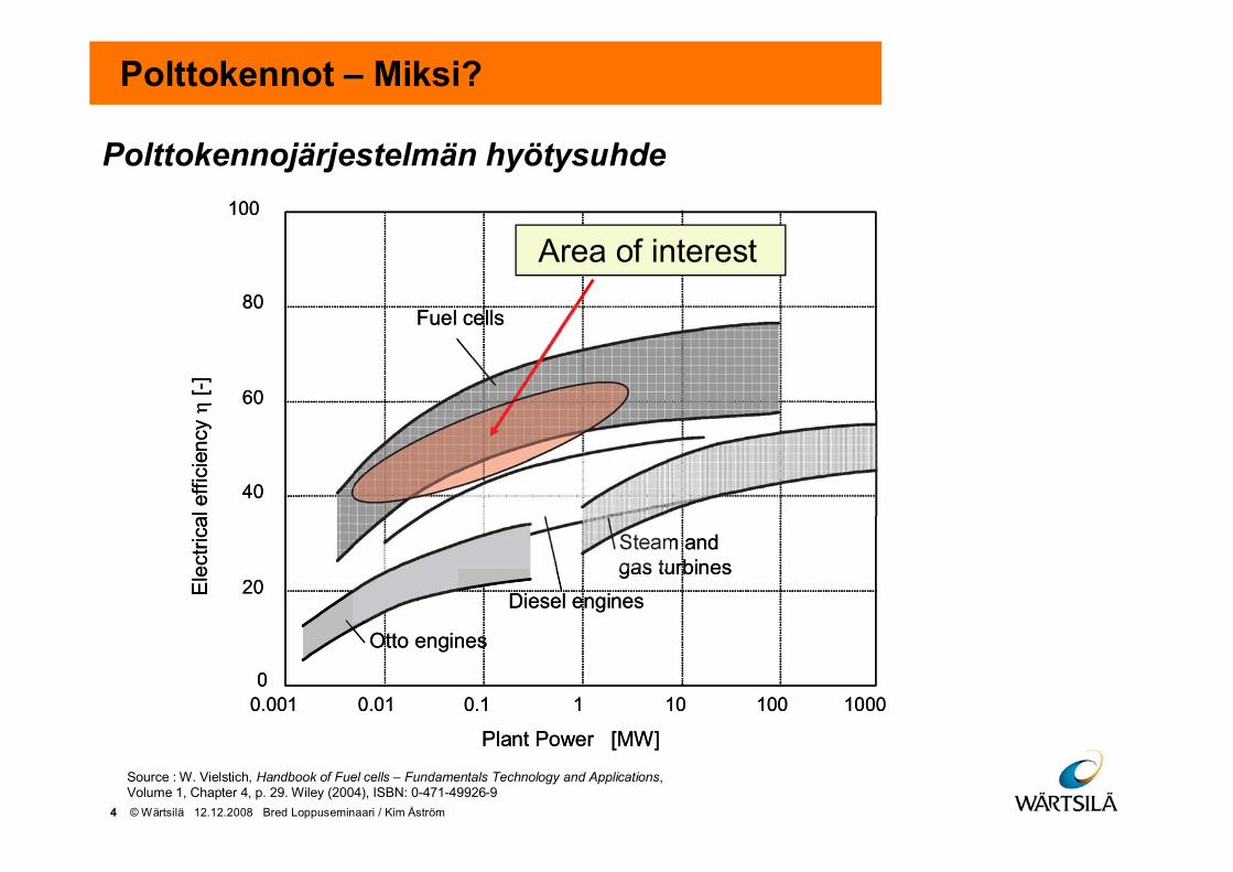
4 © Wärtsilä 12.12.2008 Bred Loppuseminaari / Kim Åström
Fuel cells
Steam andgas turbines
Diesel engines
Otto engines
Ele
ctric
alef
ficie
ncy
[-]
Plant Power [MW]
100
80
60
40
20
00.001 0.01 0.1 1 10 100 1000
Fuel cells
Steam andgas turbines
Diesel engines
Otto engines
Ele
ctric
alef
ficie
ncy
[-]
Plant Power [MW]
100
80
60
40
20
00.001 0.01 0.1 1 10 100 1000
Polttokennojärjestelmän hyötysuhde
Area of interest
Source : W. Vielstich, Handbook of Fuel cells – Fundamentals Technology and Applications,Volume 1, Chapter 4, p. 29. Wiley (2004), ISBN: 0-471-49926-9
Polttokennot – Miksi?
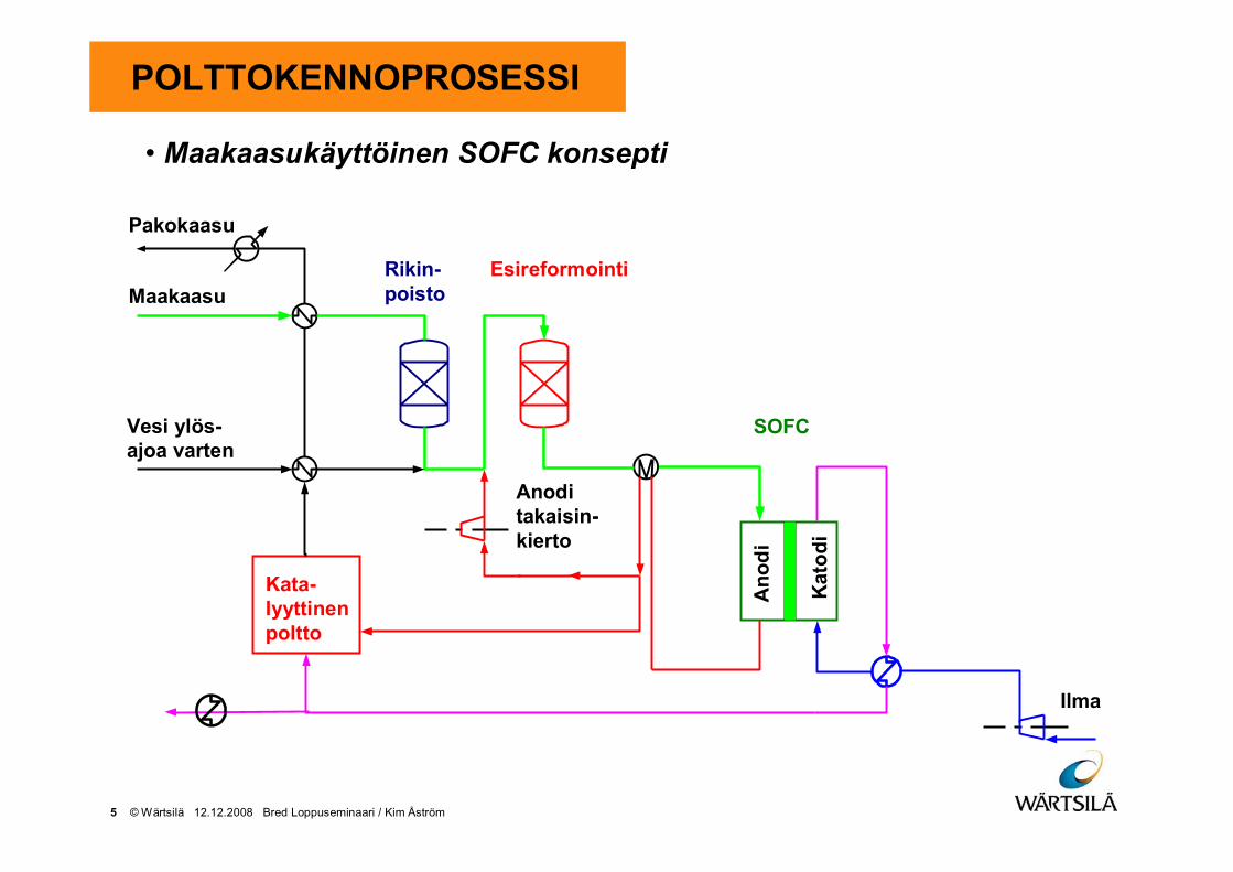
5 © Wärtsilä 12.12.2008 Bred Loppuseminaari / Kim Åström
POLTTOKENNOPROSESSI
Kata-lyyttinenpoltto
Ilma
SOFC
Ano
di
Kat
odi
Anoditakaisin-kierto
Vesi ylös-ajoa varten
Maakaasu
Pakokaasu
Rikin-poisto
Esireformointi
• Maakaasukäyttöinen SOFC konsepti

6 © Wärtsilä 12.12.2008 Bred Loppuseminaari / Kim Åström
Wärtsilä Fuel Cell Program
SOFC 1 - 5 kW test systemNG, 2004, > 7000 h in operation
WFC20 -prototype20 kW, NG, > 1000 h
e > 42 % 2006 - 2007
WFC20, WFC5020 – 50 kW,NG, methanol, Bio gas
e > 45 %2007 - 2010
WFC250250 kWe,NG, methanol, bio gas
e ~50 %
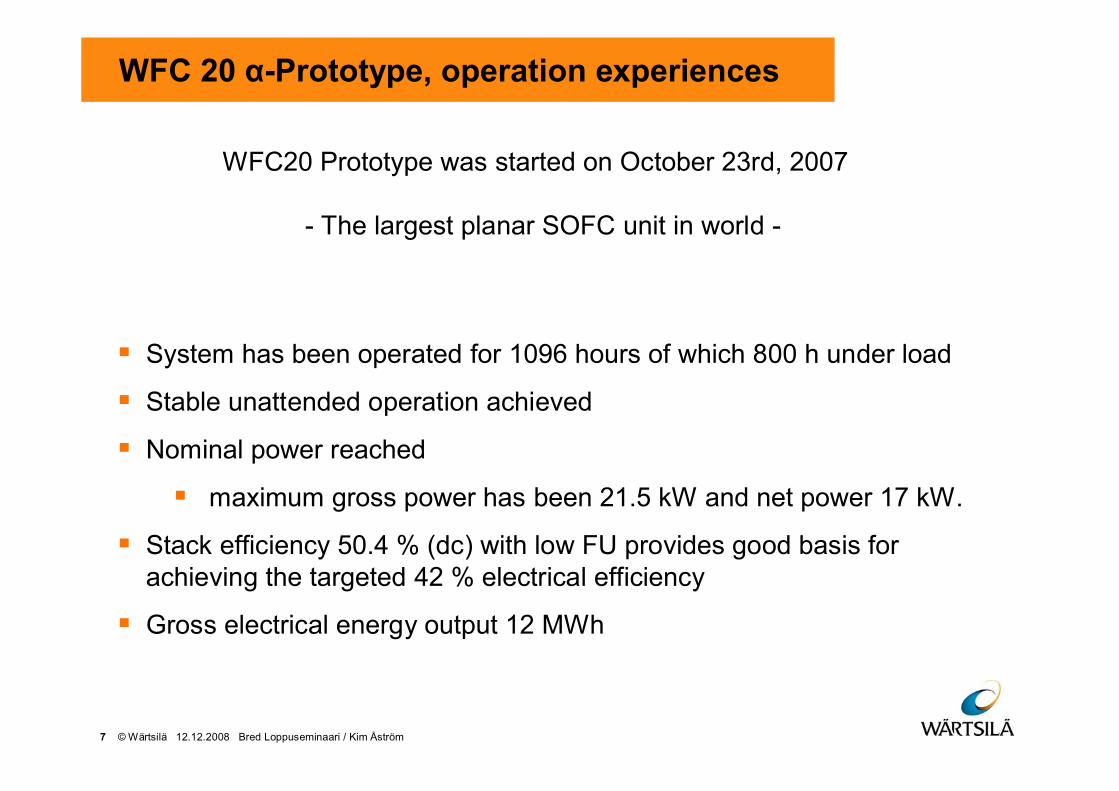
7 © Wärtsilä 12.12.2008 Bred Loppuseminaari / Kim Åström
WFC 20 -Prototype, operation experiences
System has been operated for 1096 hours of which 800 h under load
Stable unattended operation achieved
Nominal power reached
maximum gross power has been 21.5 kW and net power 17 kW.
Stack efficiency 50.4 % (dc) with low FU provides good basis forachieving the targeted 42 % electrical efficiency
Gross electrical energy output 12 MWh
WFC20 Prototype was started on October 23rd, 2007
- The largest planar SOFC unit in world -

8 © Wärtsilä 12.12.2008 Bred Loppuseminaari / Kim Åström
Alpha gross electric power output during 1096h
Burnerbroken
Short circuit inhot box
Anode recyclepump broken
Nominal power
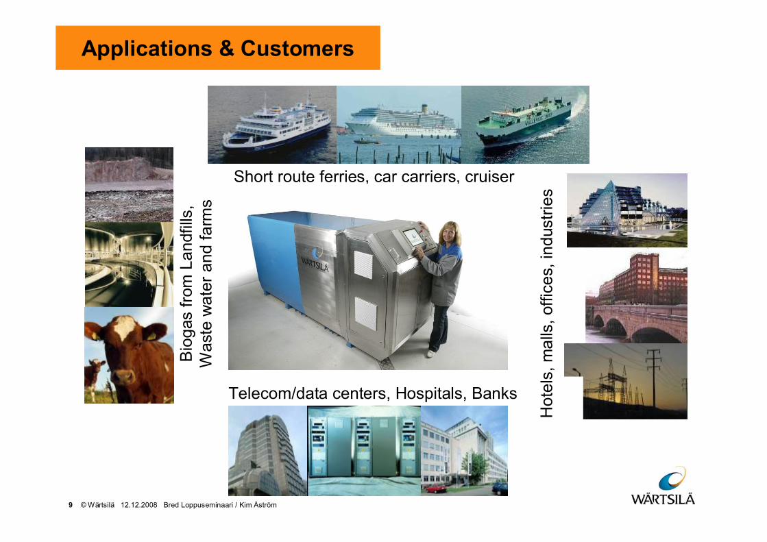
9 © Wärtsilä 12.12.2008 Bred Loppuseminaari / Kim Åström
Applications & Customers
Hot
els,
mal
ls, o
ffic
es, i
ndus
trie
s
Telecom/data centers, Hospitals, Banks
Short route ferries, car carriers, cruiserB
ioga
s fr
om L
andf
ills,
Was
te w
ater
and
farm
s

10 © Wärtsilä 12.12.2008 Bred Loppuseminaari / Kim Åström
LUOTETTAVUUSANALYYSI
Järjestelmän luotettavuusanalyysityö aloitettiin vuonna 2005
Lähtökohdat:• Luotettavuus ja elinikä keskeisiä tuotteen kilpailukyvyn kannalta
• Monimutkainen järjestelmä => tarvitaan systemaattisia menetelmiäkokonaisuuden hahmottamiseksi
• Riittävä luotettavuus/käytettävyys edellytys jo protovaiheessa
Alustavat tavoitteet:• Menetelmien kartoitus ja valinta
• Menetelmien käyttöönotto
• Järjestelmäkomponenttien luotettavuuden kartoitus
• Alustavien luotettavuusennusteiden määrittäminen
• Alustavat vaatimukset komponenttien luotettavuudelle
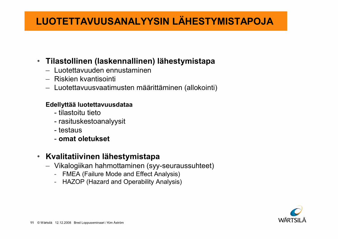
11 © Wärtsilä 12.12.2008 Bred Loppuseminaari / Kim Åström
LUOTETTAVUUSANALYYSIN LÄHESTYMISTAPOJA
• Tilastollinen (laskennallinen) lähestymistapa– Luotettavuuden ennustaminen– Riskien kvantisointi– Luotettavuusvaatimusten määrittäminen (allokointi)
Edellyttää luotettavuusdataa- tilastoitu tieto- rasituskestoanalyysit- testaus- omat oletukset
• Kvalitatiivinen lähestymistapa– Vikalogiikan hahmottaminen (syy-seuraussuhteet)
- FMEA (Failure Mode and Effect Analysis)- HAZOP (Hazard and Operability Analysis)

12 © Wärtsilä 12.12.2008 Bred Loppuseminaari / Kim Åström
KÄYTETTY LÄHESTYMISTAPA
• Laadittiin FMEA kaikille järjestelmän keskeisille komponenteille– Komponettien vikaantumismekanismit ja näiden seuraukset
– Vikojen havaittavuus
– Kriittiset tapahtumaketjut
• FMEA:n pohjalta laadittiin vikapuu– Fokus vioissa joista voi seurata järjestelmän alasajo
• Vikapuun pohjalta simuloitiin järjestelmän vikakäyttäytymistädynaamisessa mallissa– Pohjana karkeat arviot komponenttien vikajakaumista
• Varsinaiset polttokennot käsiteltiin erikseen

13 © Wärtsilä 12.12.2008 Bred Loppuseminaari / Kim Åström
VIKAPUUANALYYSI
• Vikapuun komponentit: juurisyyt ja seuraukset
• Yhdistetään Boolen logiikalla + satunnaisparametreilla
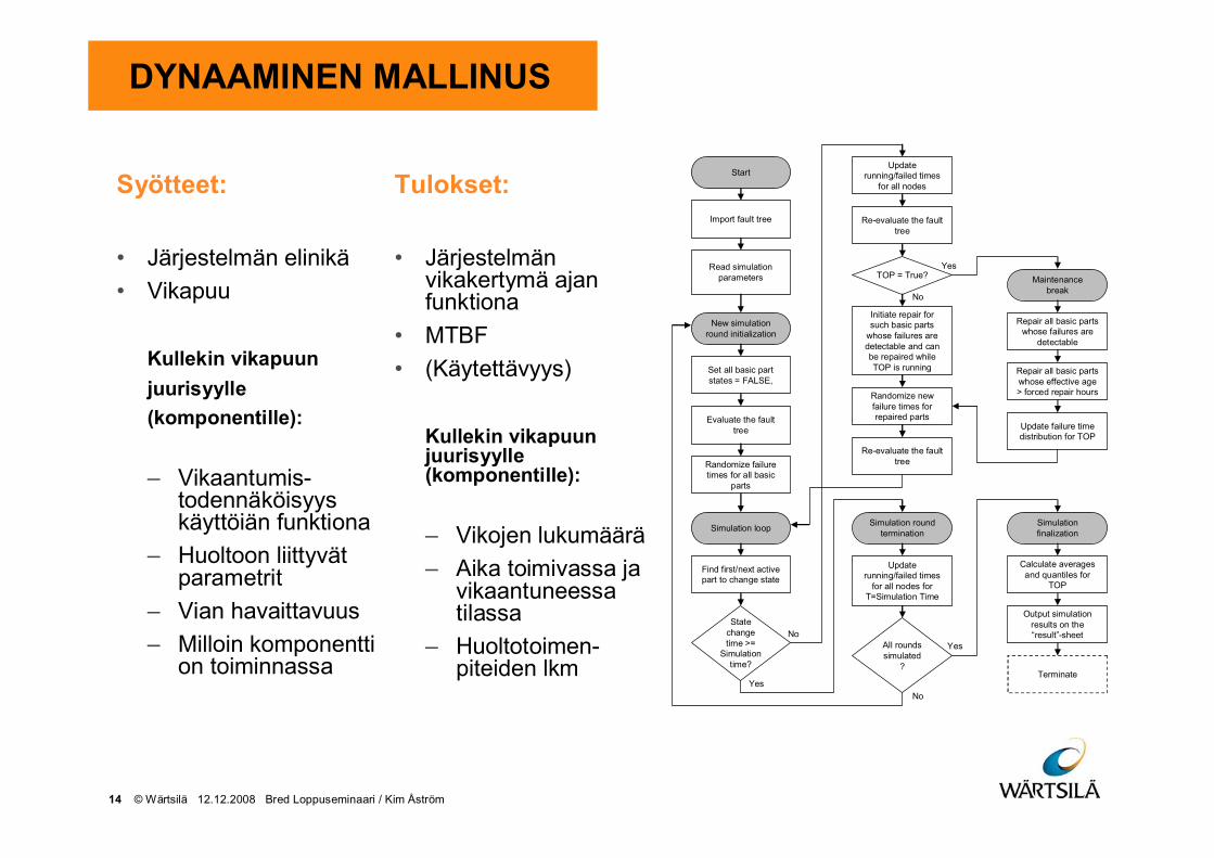
14 © Wärtsilä 12.12.2008 Bred Loppuseminaari / Kim Åström
DYNAAMINEN MALLINUS
Start
Import fault tree
Read simulationparameters
New simulationround initialization
Set all basic partstates = FALSE,
Evaluate the faulttree
Randomize failuretimes for all basic
parts
Find first/next activepart to change state
Simulation loop
Statechangetime >=
Simulationtime?
Updaterunning/failed times
for all nodes
Re-evaluate the faulttree
TOP = True?
Repair all basic partswhose failures are
detectable
Repair all basic partswhose effective age> forced repair hours
Re-evaluate the faulttree
Maintenancebreak
Update failure timedistribution for TOP
Initiate repair forsuch basic parts
whose failures aredetectable and canbe repaired whileTOP is running
Updaterunning/failed times
for all nodes forT=Simulation Time
Simulation roundtermination
All roundssimulated
?
Simulationfinalization
Calculate averagesand quantiles for
TOP
Output simulationresults on the“result”-sheet
Terminate
Randomize newfailure times forrepaired parts
Yes
Yes
Yes
No
No
No
Syötteet:
• Järjestelmän elinikä
• Vikapuu
Kullekin vikapuunjuurisyylle(komponentille):
– Vikaantumis-todennäköisyyskäyttöiän funktiona
– Huoltoon liittyvätparametrit
– Vian havaittavuus
– Milloin komponenttion toiminnassa
Tulokset:
• Järjestelmänvikakertymä ajanfunktiona
• MTBF
• (Käytettävyys)
Kullekin vikapuunjuurisyylle(komponentille):
– Vikojen lukumäärä
– Aika toimivassa javikaantuneessatilassa
– Huoltotoimen-piteiden lkm
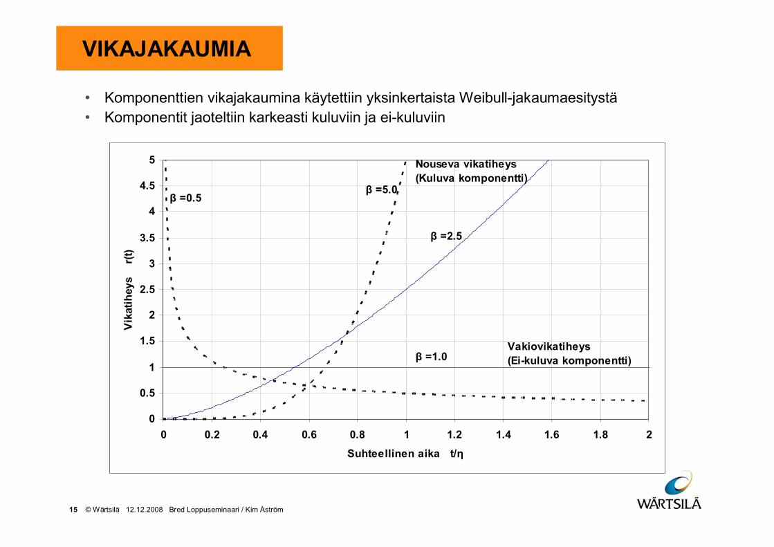
15 © Wärtsilä 12.12.2008 Bred Loppuseminaari / Kim Åström
VIKAJAKAUMIA
• Komponenttien vikajakaumina käytettiin yksinkertaista Weibull-jakaumaesitystä• Komponentit jaoteltiin karkeasti kuluviin ja ei-kuluviin
0
0.5
1
1.5
2
2.5
3
3.5
4
4.5
5
0 0.2 0.4 0.6 0.8 1 1.2 1.4 1.6 1.8 2
Suhteellinen aika t/
Vik
atih
eys
r(
t)
=0.5
=1.0
=2.5
=5.0
Vakiovikatiheys(Ei-kuluva komponentti)
Nouseva vikatiheys(Kuluva komponentti)
16 © Wärtsilä 12.12.2008 Bred Loppuseminaari / Kim Åström
TIETOLÄHTEITÄ
• Lukuisia luotettavuusdataa luettelevia tietolähteitä olemassa esim.
– OREDA Offshore Reliability Data
– SINTEF Reliability Data for Safety Instrumented Systems
– EXIDA Safety Equipment Reliability Handbook
– T-book Reliability Data of Components in Nordic Nuclear Plants
Tiedon sovellettavuuteen yleensä syytä suhtautua varauksellisesti
• Komponenttivalmistajat
• Oletukset ja omat arvioinnit
• Huoltoraportit, kokemukset “kentältä”

17 © Wärtsilä 12.12.2008 Bred Loppuseminaari / Kim Åström
TULOKSIA, ESIMERKKI
20 kW vikajakauma, 40000h simuloitu, yhteensä9.1 alasajoa (MTBF = 4400h)
0
1
2
3
4
5
6
7
8
9
10
Kes
kim
äärä
inen
vik
ojen
lkm
Muut komponentit
Pumput, kompressorit
Putket, lämmönvaihtimetja reaktorit
Venttiilit
Lämpötila-anturit
Muu automaatio jainstrumentointi
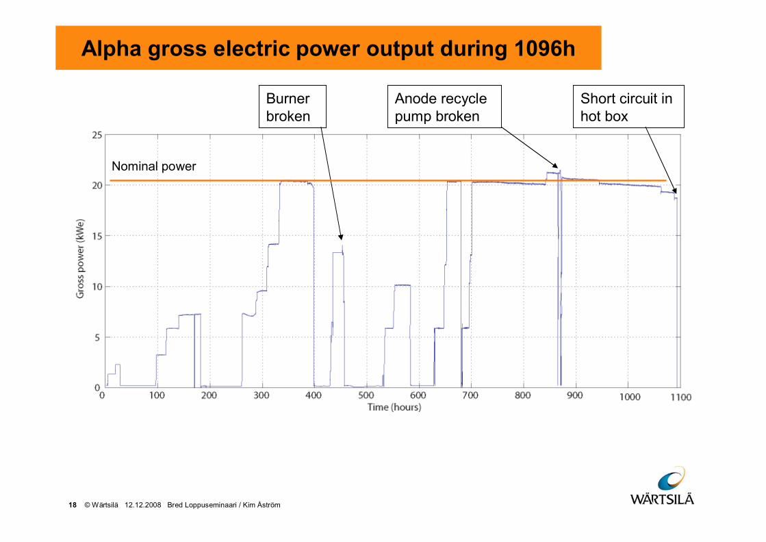
18 © Wärtsilä 12.12.2008 Bred Loppuseminaari / Kim Åström
Alpha gross electric power output during 1096h
Burnerbroken
Short circuit inhot box
Anode recyclepump broken
Nominal power

19 © Wärtsilä 12.12.2008 Bred Loppuseminaari / Kim Åström
POLTTOKENNOJEN LUOTETTAVUUS
• Järjestelmässä 24 polttokenno”stäckiä” keskenäisessävuorovaikutuksessa
• Polttokennojen degradaatio on tunnustettu ilmiö, luotettavuudesta(äkillinen vikaantuminen) ei ole tietoa
• Ymmärrys luotettavuudesta on keskeinen tieto polttokennojenyhteenliittämisen ja kaasusyöttötopologian suunnittelussa
• Fysikaaliset degradaatioon / vikaantumiseen liittyvät ilmiöt liianmonimutkaisia käytettäväksi luotettavuusanalyysissä
• Semi-kvalitatiivisen mallin avulla voidaan tutkia keskeistenluotettavuusparametrien vaikutuksia

20 © Wärtsilä 12.12.2008 Bred Loppuseminaari / Kim Åström
Stack Reliability, Simple Qualitative Model
r1(t1)
Fullyfunctional
Partial / minorfailure
Critical failureSystem
shutdown
Systemtriggered
r0(t0)
Ps1-Ps
AND
OR
Start-upfailure
Minorfailure
r0
Criticalfailure
r1
[Start-up]
P = 1-Ps
Runtime failure
TOP(Stack induced system failure)
0 0 0 1activated by r0
=10 =1
Model parameters:
r0 0 )
r1 1 )
=Weibull scale factor
=Weibull shape factor
Ps=Probability of surviving thermocycle
75.2,89.01,1
11MTTF
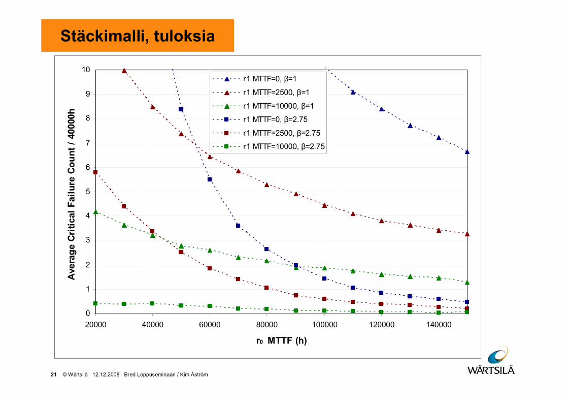
21 © Wärtsilä 12.12.2008 Bred Loppuseminaari / Kim Åström
Stäckimalli, tuloksia
0
1
2
3
4
5
6
7
8
9
10
20000 40000 60000 80000 100000 120000 140000
r0 MTTF (h)
Ave
rage
Cri
tical
Fai
lure
Cou
nt /
4000
0hr1 MTTF=0, =1
r1 MTTF=2500, =1
r1 MTTF=10000, =1
r1 MTTF=0, =2.75
r1 MTTF=2500, =2.75
r1 MTTF=10000, =2.75
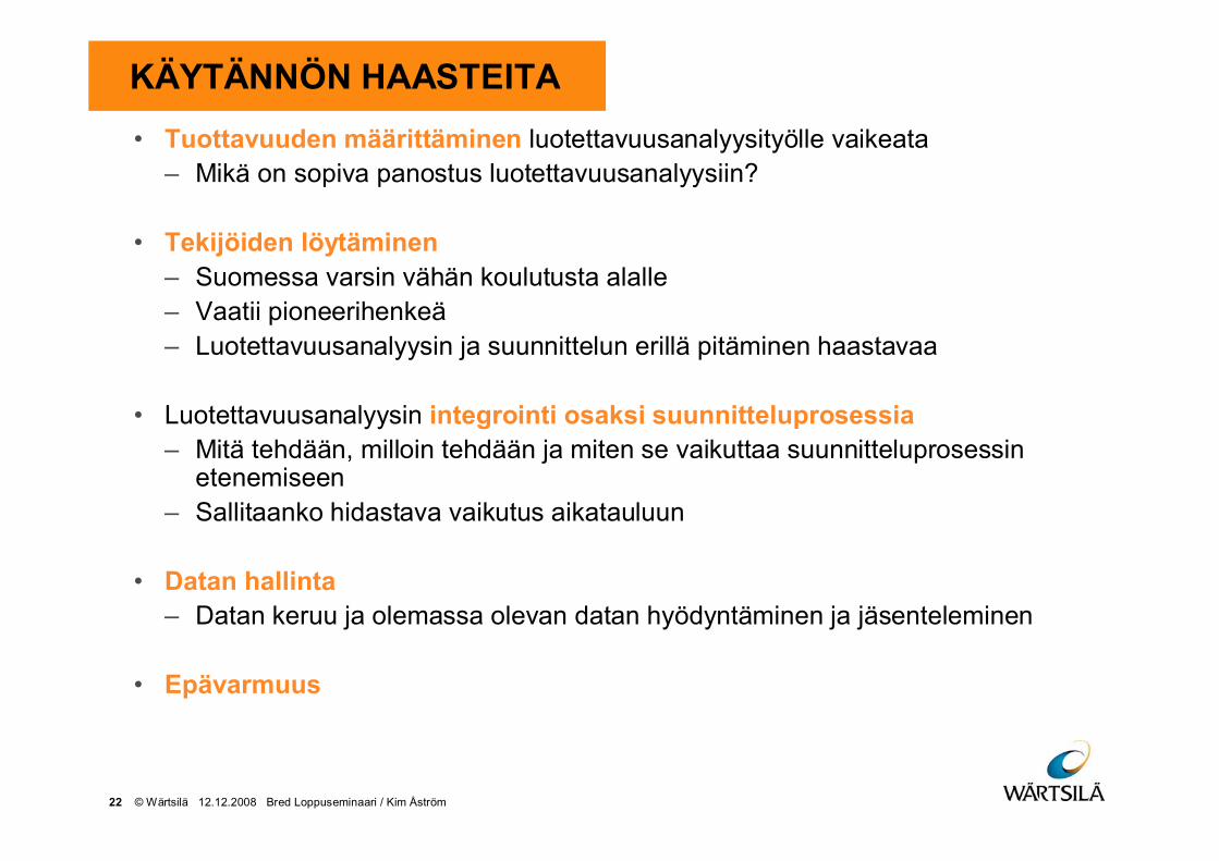
22 © Wärtsilä 12.12.2008 Bred Loppuseminaari / Kim Åström
KÄYTÄNNÖN HAASTEITA• Tuottavuuden määrittäminen luotettavuusanalyysityölle vaikeata
– Mikä on sopiva panostus luotettavuusanalyysiin?
• Tekijöiden löytäminen– Suomessa varsin vähän koulutusta alalle– Vaatii pioneerihenkeä– Luotettavuusanalyysin ja suunnittelun erillä pitäminen haastavaa
• Luotettavuusanalyysin integrointi osaksi suunnitteluprosessia– Mitä tehdään, milloin tehdään ja miten se vaikuttaa suunnitteluprosessin
etenemiseen– Sallitaanko hidastava vaikutus aikatauluun
• Datan hallinta– Datan keruu ja olemassa olevan datan hyödyntäminen ja jäsenteleminen
• Epävarmuus
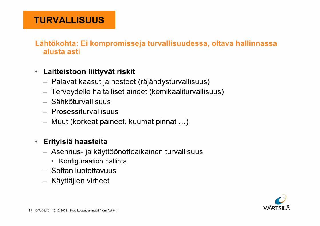
23 © Wärtsilä 12.12.2008 Bred Loppuseminaari / Kim Åström
TURVALLISUUS
Lähtökohta: Ei kompromisseja turvallisuudessa, oltava hallinnassaalusta asti
• Laitteistoon liittyvät riskit– Palavat kaasut ja nesteet (räjähdysturvallisuus)– Terveydelle haitalliset aineet (kemikaaliturvallisuus)– Sähköturvallisuus– Prosessiturvallisuus– Muut (korkeat paineet, kuumat pinnat …)
• Erityisiä haasteita– Asennus- ja käyttöönottoaikainen turvallisuus
• Konfiguraation hallinta
– Softan luotettavuus– Käyttäjien virheet
24 © Wärtsilä 12.12.2008 Bred Loppuseminaari / Kim Åström
System Safety management
• System Safety Programme Plan (not a project specific)– Definitions
– Objects for safety assessment
– Working practices
– Risk assessment criteria
– All the efforts shall serve the same goal
– If possible, all the results from different analyses should be commensurable
– It is beneficial if other disciplines could be integrated with safety tasks
SystemSafety
ProgrammePlan
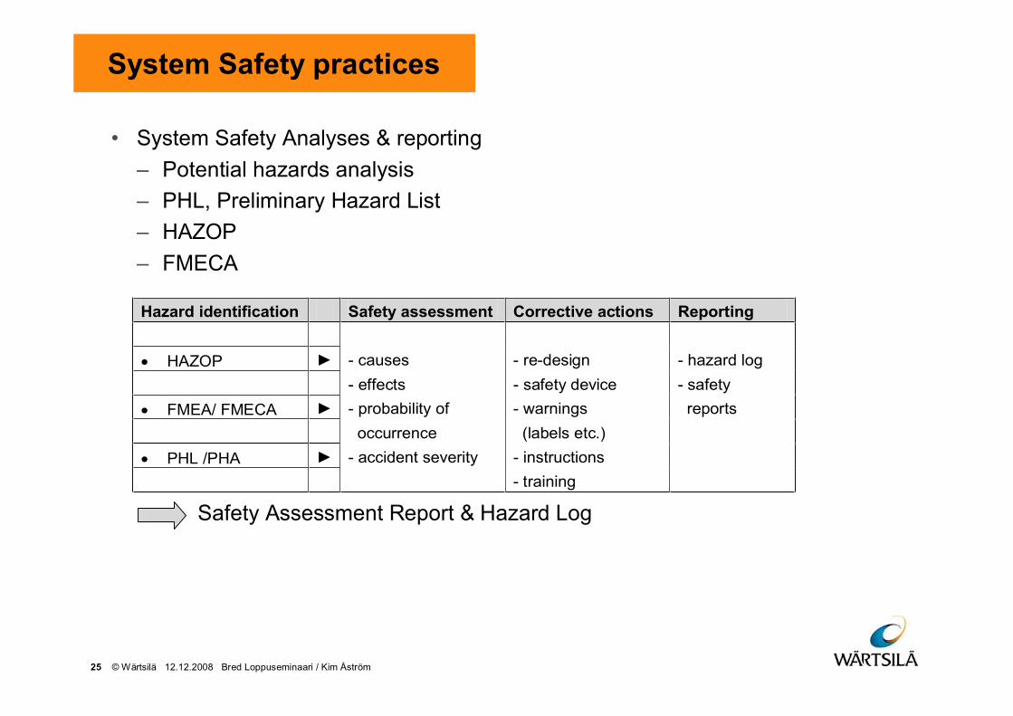
25 © Wärtsilä 12.12.2008 Bred Loppuseminaari / Kim Åström
System Safety practices
• System Safety Analyses & reporting
– Potential hazards analysis
– PHL, Preliminary Hazard List
– HAZOP
– FMECA
Safety Assessment Report & Hazard Log
Hazard identification Safety assessment Corrective actions Reporting
HAZOP - causes - re-design - hazard log
- effects - safety device - safety
FMEA/ FMECA - probability of - warnings reports
occurrence (labels etc.)
PHL /PHA - accident severity - instructions
- training

26 © Wärtsilä 12.12.2008 Bred Loppuseminaari / Kim Åström
Comparison of analyses
Method Risk identification is based on Strenghts Weaknesses
PHL/PHA
SFS-EN 1050 "Safety of machinery.Principles for risk assessment."Appendix A: List of potentialhazards, hazardous situations andhazardous events.
Easy and fast method,inherent features
no process-risks, man-machineinterfaces, erroneous actions
HAZOPThe hazards and operationalconcerns of a system
The process deviationsare systematicallyanalysed
A human-intensive activity,inherent risks are notnecessarily identified
Design FMECAEach assembly is analysed part bypart
Failure modes which willhamper functionality
Time-consuming analysis
Process /sequenceFMECA
The process is analysed step bystep to find abnormal events
Failure modes related toprocess
Time-consuming analysis
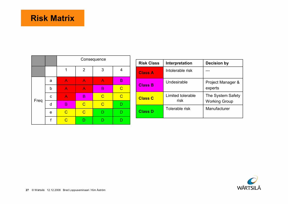
27 © Wärtsilä 12.12.2008 Bred Loppuseminaari / Kim Åström
Risk Matrix
DDDCf
DDCCe
DCCBd
CCBAc
CBAAb
BAAAa
Freq
4321
Consequence
ManufacturerTolerable riskClass D
The System SafetyWorking Group
Limited tolerableriskClass C
Project Manager &experts
UndesirableClass B
---Intolerable riskClass A
Decision byInterpretationRisk Class

28 © Wärtsilä 12.12.2008 Bred Loppuseminaari / Kim Åström
Results
• Personnel hazards. Tot 34 pcs, 25% of 138
• System hazards. Tot 90 pcs, 65% of 138
• Environment hazards. Tot 14 pcs, 10% of 138
Consequence1 2 3 4
a
b 1 1
c 1 2
d 5 6 3
e 5 3 1 2Fre
quen
ce
f 1 1 1 1
Consequence1 2 3 4
a
b 1 1
c 1 6 3
d 16 16 5
e 5 15 5 1Fre
quen
ce
f 1 10 3 1
Consequence1 2 3 4
a
b 1
c 4
d 2 3
e 2Fre
quen
ce
f 1 1
29 © Wärtsilä 12.12.2008 Bred Loppuseminaari / Kim Åström
KOKEMUKSET & LOPPUPÄÄTELMÄT
• Prototyyppiasteessa olevan teknologian luotettavuusanalyysi on pitkälti uusikonsepti
Parhaiten soveltuvat menetelmät ja käytännöt haettava empiirisesti
• Kvalitatiivisista menetelmistä (FMEA, HAZOP) eniten konkreettista hyötyä– Etenkin automaation suunnitteluun runsaasti syötettä– HAZOP turvallisuuden kannalta välttämätön, luotettavuuden kannalta ei
FMEAn veroinen
• Kvantitatiivisten analyysien ja niiden edellyttämän datan välillä ”muna-kana”problematiikka
• Prototyypille (käyttö)kokemuksen perusteella keskeiset luotettavuusongelmatovat ilmeisiä ilman tarvetta analyyseille.
• Turvallisuusanalyyseissä runsaasti työnsarkaa

Seminar 12.12.2008
Kalle Lehtinen
BRED project resultsBRED project results

Evaluating equipment reliability effects on warranty and service contracts
• Purpose is evaluate how a change in design or production will affect warranty and service contract production costs
• Do we get the money invested in reliability back?
• Interaction between service and new sales
• Calculation for reliability investment payback
• Focus on one equipment, part of equipment or single design change
• Critical parts can be analyzed individually by taking account failure tendency of the part but including failure related costs for the complete equipment
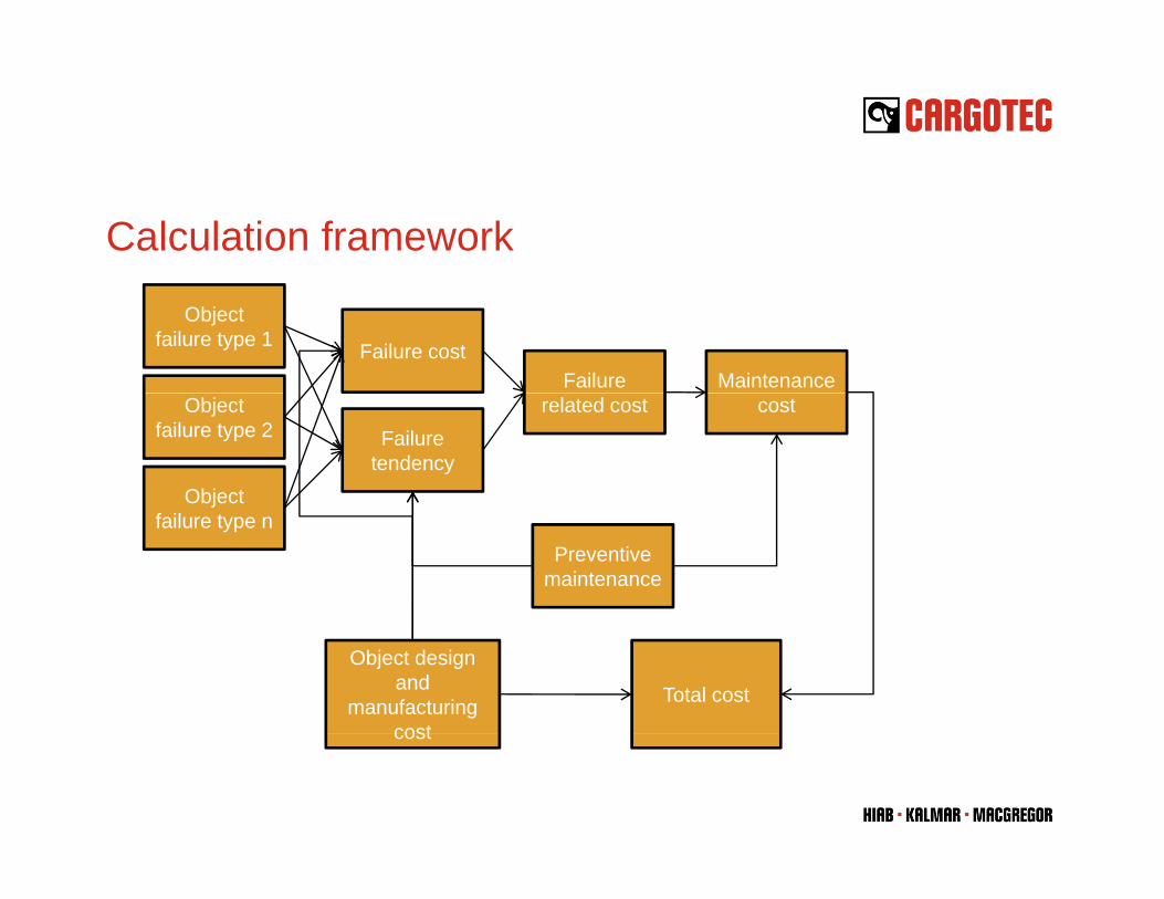
Calculation framework
Object failure type 1 Failure cost
Failure Maintenance Object
failure type 2 Failure tendency
related cost
Object
cost
Preventive maintenance
jfailure type n
Object design and
manufacturing cost
Total cost
cost
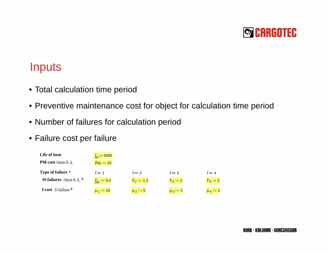
Inputs
• Total calculation time period
• Preventive maintenance cost for object for calculation time period
• Number of failures for calculation period
• Failure cost per failure
Life of item L 5400:=
PM-cost /item 0..L Pm 20:=
Type of failure a f 1 f 2 f 3 f 4
#f-failures /item 0..L b F1 0.4:= F2 1.2:= F3 2:= F4 2:=
f-cost /f-failure d μ1 10:= μ2 5:= μ3 2:= μ4 2:=
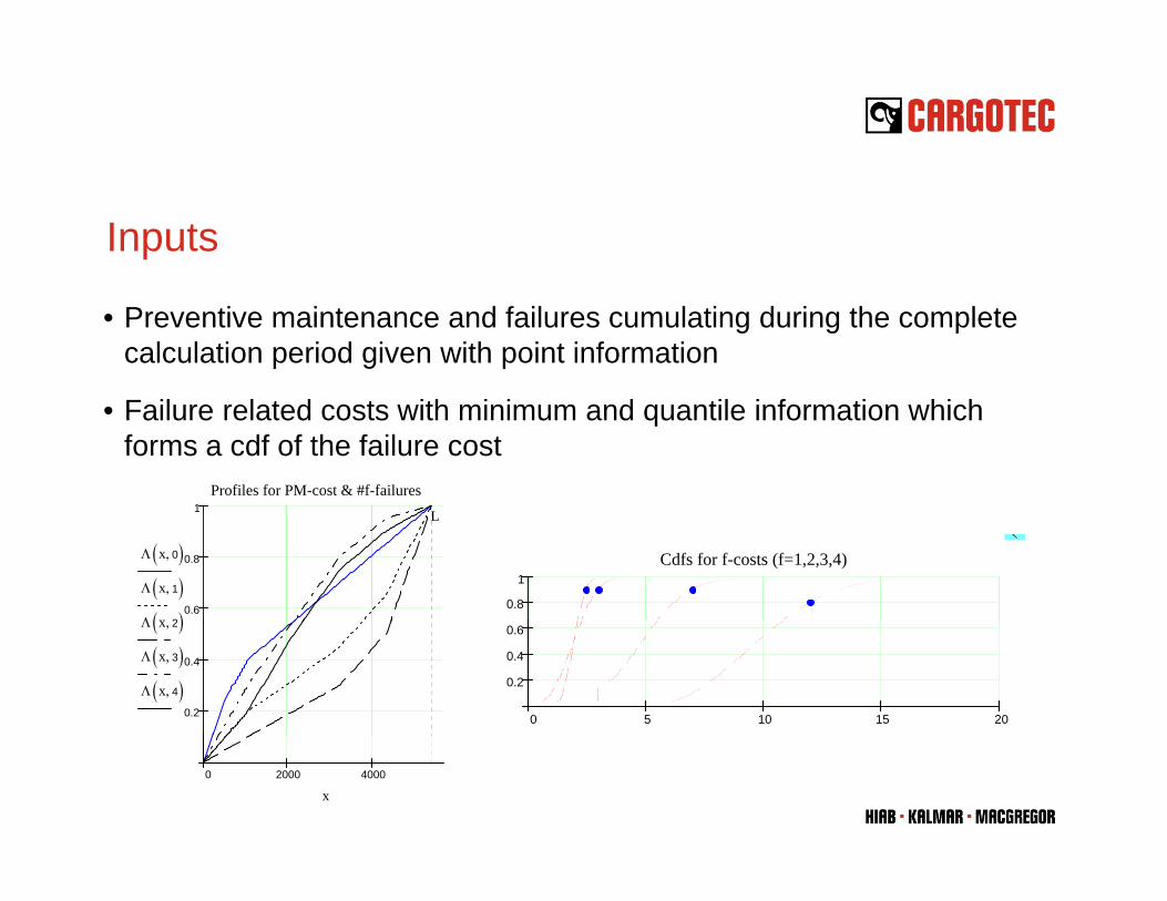
Inputs
• Preventive maintenance and failures cumulating during the complete calculation period given with point information
• Failure related costs with minimum and quantile information which forms a cdf of the failure cost
1Profiles for PM-cost & #f-failures
0.6
0.8
1
Λ x 0,( )Λ x 1,( )Λ x 2( )
L⎝
0.8
1Cdfs for f-costs (f=1,2,3,4)
0.2
0.4
Λ x 2,( )Λ x 3,( )Λ x 4,( )
0 5 10 15 20
0.2
0.4
0.6
0 2000 4000
x

Inputs
• Warranty and service contract periods are given within the total calculation period
• For each period the division of costs between the manufacturer and customer is given
• The division is formed based proposed service contract modelThe division is formed based proposed service contract model
• Service contract can also be taken into account when failure tendency is estimated

Results• Preventive maintenance costsPreventive maintenance costs
• Failure related costs in each time period
• By comparing different solutions and their design and productionBy comparing different solutions and their design and production costs the most economical solution can be found
0.8
1Cdf for Warranty FR costs
FR L 0,( ) £00.8
1Cdf for Service1 FR costs
FR L 1,( ) £1
0 5 10
0.2
0.4
0.6
0 1 2 3 4
0.2
0.4
0.6
0 4
0.6
0.8
1Cdf for Service2 FR costs
FR L 2,( ) £2
0 4
0.6
0.8
1Cdf for Service3 FR costs
FR L 3,( ) £3
0 10 20 30
0.2
0.4
0 5 10 15 20
0.2
0.4
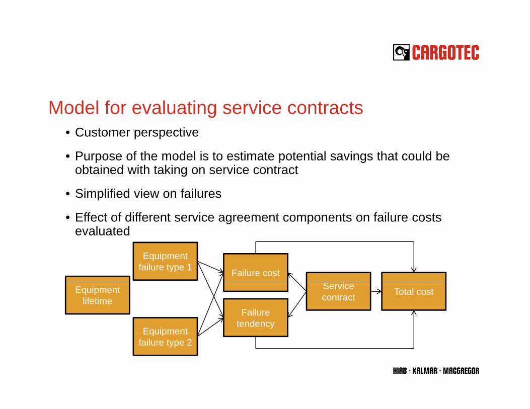
Model for evaluating service contracts• Customer perspective
• Purpose of the model is to estimate potential savings that could be obtained with taking on service contract
• Simplified view on failures
• Effect of different service agreement components on failure costs evaluatedevaluated
Equipment failure type 1 Failure cost
Equipment lifetime
Equipment
Failure tendency
Service contract Total cost
Equipment failure type 2
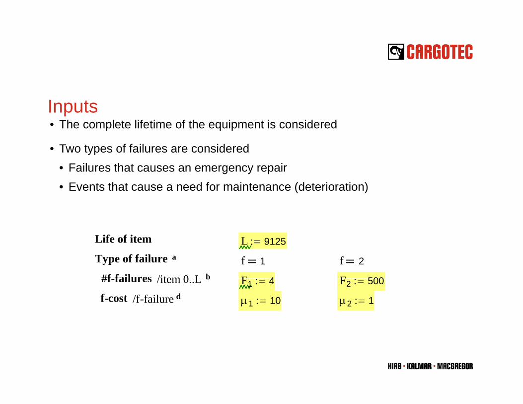
Inputs• The complete lifetime of the equipment is consideredThe complete lifetime of the equipment is considered
• Two types of failures are considered• Failures that causes an emergency repair• Events that cause a need for maintenance (deterioration)
Life of item L 9125:=
Type of failure a f 1 f 2
#f failures /item 0 L b F 4 F 500 #f-failures /item 0..L b F1 4:= F2 500:=
f-cost /f-failure d μ1 10:= μ2 1:=
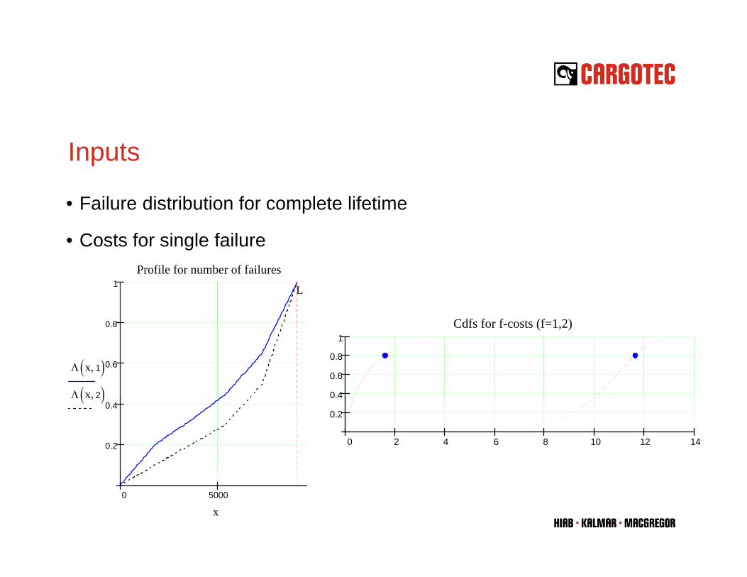
Inputs
• Failure distribution for complete lifetime
• Costs for single failure
0 8
1Profile for number of failures
L
Cdfs for f-costs (f=1 2)
0.6
0.8
Λ x 1,( )Λ x 2,( ) 0.4
0.6
0.8
1Cdfs for f-costs (f 1,2)
0.2
0.4Λ x 2,( )
0 2 4 6 8 10 12 14
0.2
0.4
0 5000
x
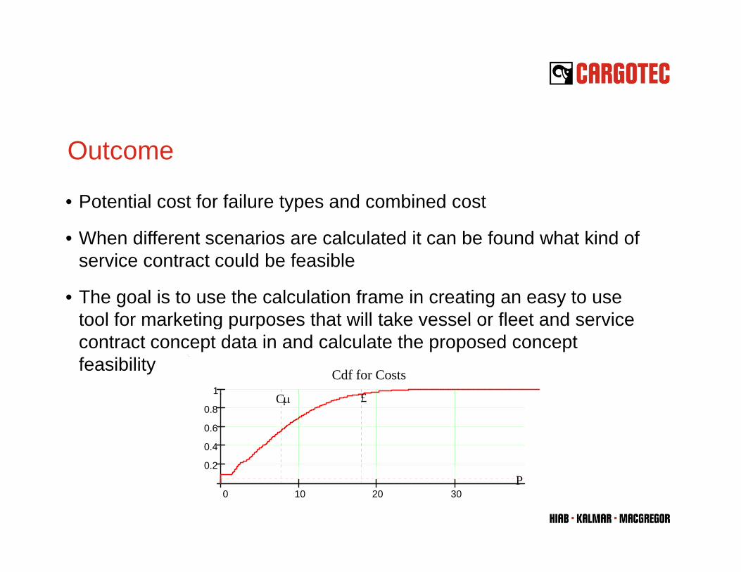
Outcome
• Potential cost for failure types and combined cost
• When different scenarios are calculated it can be found what kind of service contract could be feasible
• The goal is to use the calculation frame in creating an easy to use tool for marketing purposes that will take vessel or fleet and servicetool for marketing purposes that will take vessel or fleet and service contract concept data in and calculate the proposed concept feasibility
1Cdf for Costs
C £
0 2
0.4
0.6
0.8Cμ £
0 10 20 30
0.2P
Failure tendency modeling using group method
• Method was created to handle data reliability data that does not have information on any specific part but from a group of similar parts
• For example pumps in group which we know that some of the pumps have been replaced
• Method also provides a mean for censoring the data if there is lots ofMethod also provides a mean for censoring the data if there is lots of uncertainty about data quality from beginning or from the end of the calculation period
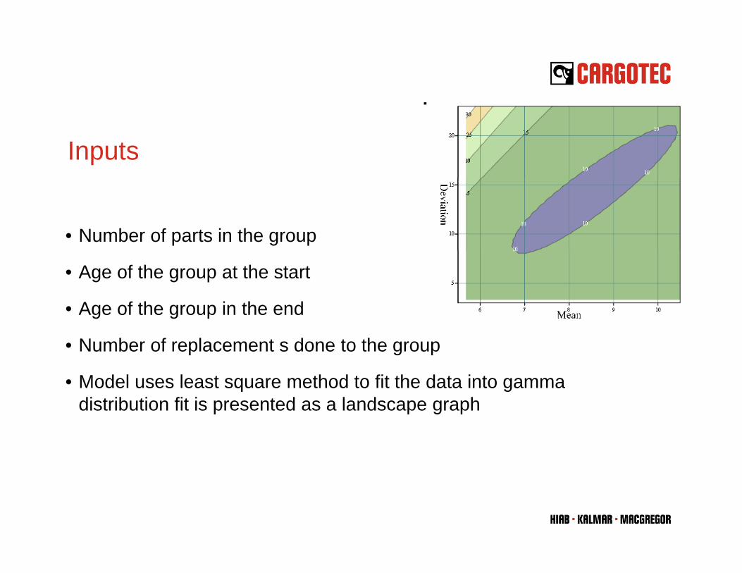
Inputs
• Number of parts in the group
• Age of the group at the start
• Age of the group in the end
• Number of replacement s done to the group
• Model uses least square method to fit the data into gamma distribution fit is presented as a landscape graph

Results
• As a result model provides the distributions optimum mean and deviation
• From the distribution numerous different results can be calculated which can then be used further
10Renewal function
0 6
0.8
1CDF of failure age
ility
μ
5
10
ber o
f fai
lure
s
Λ x μ, σ,( )
0 20 40 60 80
0.2
0.4
0.6
Prob
abi
F x 1, μ, σ,( )
0 20 40 60 80
Mea
n nu
mb
0 20 40 60 80
Age
x Age
x
Lessons learned
• Combination of engineering and financing analyses provides good results
• It’s all about processes – if don’t know what you are doing you cannot analyze and improve it
• Circle of insufficient data -> no analyses -> no need for data needsCircle of insufficient data > no analyses > no need for data needs to be broken

�
Nimike - Title
KOTEL 256: Integrated Business and Technical Product Reliability Design
Tiivistelmä – Abstract
The traditional and still dominating method for product design is focused on optimising the technical performance of a product. The reason for this is simple, there is no easily available and comprehensive design method or tool to integrate the reliability and maintainability (R&M) considerations and effects in product design.
As more the companies’ management have experienced the meaning of Product’s R&M as competitive factors in their business, as more they have started to invest R&M engineering and development. This was also a starting point from where this project was launched.
The purpose of the project was to develop a design methodology that includes the interactions and links between the customer needs, the manufacturer business targets and the product R&M performance. This makes it possible to find and simulate in detail, which are the specific customer product R&M requirements and what influence the R&M performance has on the customer satisfaction. The method enables product R&M facts to be taken into account at business decision level.
Results of the project are presented in the following appendixes: 1) Publications, 2) Master Thesis, 3) Developed Models and 4) Case-Studies; Companies Presentations.
Avainsanat - Key words reliability design, product development,
Kieli - Language English
Sivuja - Pages 181
Tyyppi - Type Project report
Laatinut - Compiled by KOTEL 042 BRED project manager professor Seppo Virtanen, Tampere University of Technology
Hyväksytty - Approved
31.12.2008
Tarkasti - Inspected by
AT
Korvaa - Replaces
Julkaisija ja jakelu - Published and distributed by
Elektroniikan tutkimuksen ja kehityksen yhteistyöelin KOTEL ry c/o VTT
PL 1000, 02044 VTT