integrated reliability and sizing optimization of a large

Wayne State University

Civil and Environmental Engineering FacultyResearch Publications Civil and Environmental Engineering

4-1-2009

Integrated Reliability and Sizing Optimization of aLarge Composite StructureChristopher D. EamonMississippi State University, Starkville, MS, [email protected]

Masoud Rais-RohaniMississippi State University, Starkville, MS

This Article is brought to you for free and open access by the Civil and Environmental Engineering at DigitalCommons@WayneState. It has beenaccepted for inclusion in Civil and Environmental Engineering Faculty Research Publications by an authorized administrator ofDigitalCommons@WayneState.

Recommended CitationEamon, C. D., and Rais-Rohani, M. (2009). "Integrated reliability and sizing optimization of a large composite structure." MarineStructures, 22(2), 315-334, doi: 10.1016/j.marstruc.2008.03.001Available at: https://digitalcommons.wayne.edu/ce_eng_frp/9

http://digitalcommons.wayne.edu/



https://digitalcommons.wayne.edu/ce_eng_frp

https://digitalcommons.wayne.edu/ce_eng_frp

https://digitalcommons.wayne.edu/ce_eng

Eamon and Rais-Rohani

1

Integrated Reliability and Sizing Optimization of a Large Composite Structure

Christopher D. Eamon1 and Masoud Rais-Rohani

2

Mississippi State University, Mississippi State, MS 39762

Abstract

In this paper, we present the application of probabilistic design modeling and reliability-based design

optimization (RBDO) methodology to the sizing optimization of a composite advanced submarine sail

structure under parametric uncertainty. With the help of probabilistic sensitivity analysis, the influence of

individual random variables on each structural failure mode is examined, and the critical modes are

treated as probabilistic design constraints under consistent lower bounds on the corresponding reliability

indices. Whereas the failure modes are applied to structural components in the solution of the RBDO

problem, the overall system reliability is also evaluated as a post-optimization step. The results indicate

that in comparison to a deterministic optimum design, the structural mass of the probabilistic optimum

design is slightly higher when consistent probabilistic constraints are imposed, and the overall structural

stiffness is found to be more critical than individual component laminate ply thicknesses in meeting the

specified design constraints. Moreover, the post-optimality analysis shows that the overall system failure

probability of the probabilistic optimum design is more than 50% lower than that of the deterministic

optimal design with less than 5% penalty in structural mass.

------------------------------ 1Associate Professor, Department of Civil and Environmental Engineering, [email protected] 2Professor, Department of Aerospace Engineering, [email protected]


2

Introduction

Probabilistic modeling and reliability-based design optimization (RBDO) have gained broad

recognition in recent years as an appropriate approach for structural optimization under uncertainty. In

RBDO, a traditional deterministic structural optimization problem is replaced by a non-deterministic one

subject to a combined set of deterministic and reliability-based (probabilistic) design constraints, with a

parameter set that includes design as well as random variables. The resulting nonlinear, probabilistic

mathematical programming problem is solved for the optimal values of design variables that improve a

structural response of interest while considering the uncertainty in material, loading, sizing, and other

contributing factors.

The evaluation of failure probability or associated reliability index for each reliability-based

constraint poses a computational challenge in RBDO as the calculation of component reliability generally

requires the solution of a separate optimization problem (in random-variable space) within, often larger,

main design optimization problem (in design-variable space). When the evaluation of each limit state

function is based on the finite element analysis (FEA) of a complex structural system, the RBDO problem

becomes considerably more complicated and computationally intensive.

A significant body of RBDO related research exists and continues to grow, though a review of the

many proposed RBDO formulations is beyond the scope of this paper. Despite the advancements in this

area, few RBDO approaches applied specifically to ship structures appear in the technical literature.

Some of these include Pu et al. (1997), Leheta et al. (1997), and Brown et al. (1996). Others have

considered the reliability analysis of submarine structures without optimization (Morandi et al. 1994), or

considered structural optimization without probabilistic analysis (Jang et al. 2003).

In this paper, an RBDO algorithm is presented and applied to a complex structural system

representing an advanced submarine sail design made of glass-reinforced polymer composite materials.

The results of RBDO problem for different combinations of component reliability constraints are

examined, followed by a sensitivity analysis and the post-optimization assessment of the system

reliability.


3

Structural Reliability

Given a limit state function, g in structural reliability analysis, it is desired to find the probability P

that g is less than zero, for which a failure is indicated by

Pf = P g X( )< 0[ ] (1)

Probability of failure Pf is theoretically found by integrating the joint probability density function (PDF)

over the failure region in the probabilistic space of random variables as

Pf = f x (X)

g(X)≤0

∫ dX (2)

where fx is the joint PDF of the limit state and X is the vector of random variables in g. The failure

region is the probability space where g ≤ 0. For most practical problems, it is well known that the

formulation of fx and its integration over the failure region are typically too difficult to compute directly.

Therefore, numerous alternative methods have been developed to estimate Pf without the direct use of Eq.

(2). In general, these methods might be classified as simulation or sampling-based methods (e.g., Monte

Carlo simulation and its variants) and analytical (but numerically implemented) algorithms. The former,

although potentially highly accurate, are generally plagued by a requirement for a large number of

samples (i.e., evaluations of the limit-state function) to accurately estimate failure probability. Although

there are some exceptions with variance reduction techniques, this problem can be expected to worsen as

failure probability becomes smaller. Of the analytical approaches, the most common ones make use of

the reliability index, β, as a surrogate measure of failure probability, and bypass the direct calculation of

Pf entirely. Assuming β is computed accurately, it can be shown that a transformation to Pf can be made

by use of the standard normal cumulative distribution function, Φ such that Pf = Φ(−β) . Although

computationally efficient, these analytical methods must be used with caution as the accuracy varies with

the non-linearity of the limit state, the non-normality of the random variables, as well as other

characteristics of the limit state function (Eamon et al. 2005). The necessary requirement of these


4

methods is to locate the most probable point of failure (MPP), which typically requires an optimization

algorithm. At the MPP, the limit state is approximated with a linear or higher order formulation from

which reliability index can be calculated.

For this study, the iterative Advanced Mean Value Plus (AMV+) method is used to calculate

reliability index (Wu et al. 1990). This method is a variant of the first-order reliability method (FORM),

or Rackwitz-Fiessler procedure (Rackwitz and Fiessler 1978). In this method, the limit state function g is

repeatedly re-approximated about the MPP ( x*) until convergence, but with AMV+, an additional sub-

iteration is added on the linearized function that requires no calls to the true response. This usually allows

the MPP to converge more quickly than the Rackwitz-Fiessler algorithm, provided that the limit state

response is complex and computationally costly, as with those in this study. The specific process is as

follows:

1. The limit state is linearized using a first-order Taylor series expansion at the MPP. For the first

iteration, the mean values of random variables are used in place of the MPP. This step requires n+1 calls

to the exact limit state function, where n is the number of random variables in the problem.

g = z ≈ z(x*) +

∂z

∂Xi

i=1

n

∑x

*

Xi − xi*( ) (3)

where z(x*) is the limit state function evaluated at the MPP and represents one call to the true response

(i.e., FEA code), ∂z

∂Xi

=∂g

∂Xi

are the derivatives of the limit state function with respect to each random

variable Xi. As the limit state is an implicit function of the random variables, these derivatives are

calculated numerically using a finite difference procedure. The evaluation of each derivative requires one

call to the true response.

2. A gradient-based optimization algorithm is used to locate the MPP of the linearized function. This sub-

iteration requires no calls to the true response.


5

3. Steps 1 and 2 are repeated until MPP convergence. Typically, only several iterations are required for

convergence. At the converged MPP, reliability index can be calculated as

β =z

˜ σ z (4)

where

˜ σ g =∂z

∂Xi

2

˜ σ i2

i=1

n

∑ is the linearized standard deviation, which is a function of the random variable

standard deviations ˜ σ i :

Mathematical Formulation of the RBDO Problem

In RBDO, inherent uncertainties associated with material properties, loads, sizing, strength, and other

parameters, are captured in the mathematical formulation and solution of the optimization problem. There

are multiple ways of formulating an RBDO problem (Enevoldsen and Sorensen 1994, Frangopol 1995,

and Tu et al. 1999). In its generic form, we seek the optimal vector of design variables

Y = Y1,Y2 ,...,YNDV{ }Tthat would

min f (X,Y)

s. t. Pf i= P gi

p(X,Y) < 0[ ]≤ Pmax; i =1,N p ; (5)

Ykl ≤Yk ≤Yk

u; k =1,2,..., NDV

where f (X,Y) is the objective function of interest with dependence on design and possibly the random

variables, X = X1, X2,...,Xn{ }T . Each of the Np design constraints is expressed as a probability of

failure Pf i or, specifically, as the probability of limit state gi

p becoming negative is no greater than the

specified limit, Pmax . The design variables in Eq. (5) could be independent or represent the mean values

of a subset of random variables, with the kth design variable,Yk limited by its lower and upper bounds,

Ykl and Yk

u, respectively. For a tradeoff between design efficiency and robustness, the performance


6

function in Eq. (5) can be written as f (X,Y) = a1µ f (X,Y) + a2 ˜ σ f (X,Y), where µ f and ˜ σ f represent the

mean and standard deviation values, respectively, of the objective function, and coefficients a1 and a2

denote scalar weighting factors that signify the desired emphasis on efficiency and robustness,

respectively (Rao 1992).

By using the relationship between failure probability Pf and reliability index β , it is possible to

express the constraint limit in terms of the corresponding target or minimum reliability index as

( )max

1

min P−Φ−≈β . This relationship between Pf and β is exact when β is computed for linear limit

states containing normally distributed random variables. As noted above, for nonlinear limit states, some

accuracy is lost if a translation back to Pf is desired, although for typical problems, β usually provides

acceptable accuracy.

As is often the case, some responses such as structural weight may be marginally impacted or totally

unaffected by the variability in the random variables (i.e., design uncertainties), and consequently they

can be treated as deterministic. With weight as the objective function and a subset of design constraints as

deterministic, Eq. (5) can be rewritten as

min f (Y) =W (Y)

s.t. ˆ g ip

(X,Y) =P gi

p(X,Y) ≤ 0[ ]

Φ −βmin( )−1≤ 0; i =1,N p (6)

ˆ g jd

(µX ,Y) =Rj (µX ,Y)

Rjmax

−1≤ 0; j =1 to Nd

Ykl ≤Yk ≤Yk

u; k =1 to NDV

where ˆ g ip and ˆ g j

d represent normalized reliability-based and deterministic constraints, respectively, with

the latter preventing the critical value of a deterministic response, R j from exceeding its maximum

allowable value, R jmax. In Eqs. (6), Np and Nd represent the number of probabilistic and deterministic

constraints, respectively.


7

The presence of probabilistic design constraints makes the solution of Eq. (6) challenging and

expensive. Different approaches for the evaluation of ˆ g ip (X,Y) have been developed. In the reliability

index approach (Enevoldsen and Sorensen 1994), ˆ g ip (X,Y) is described in terms of a lower bound on the

reliability index (i.e., ˆ g ip (X,Y) =1− βi X,Y( ) βmin i

≤ 0, where βi X,Y( )= −Φ−1P gi

p(X,Y) ≤ 0[ ]

)

whereas in the performance measure approach (Tu et al. 1999), it is modeled using inverse transformation

(i.e., ˆ g ip (X,Y) = −F

G i

−1 Φ(−βmin i)( )≤ 0, where FGi

(0) = P gip

(X,Y) ≤ 0[ ]). More recently, Du and Chen

(2004) proposed the replacement of ˆ g ip (X,Y) with an equivalent deterministic constraint and the

decoupling of reliability analysis and design optimization in each design cycle whereas Qu and Haftka

(2004) suggested the use of probability safety factor in modeling of each probabilistic constraint.

The specific details regarding the application of RBDO to a complex marine structure are presented

next.

Composite Submarine Sail Structure

A new design concept envisioned for the next-generation Navy submarines replaces the current airfoil

shaped sail with a canopy style configuration known as the Composite Advanced Sail (CAS) and shown

in Fig. 1. The CAS concept is aimed at enhancing the performance of the submarine while increasing its

payload capacity. Considering the length, width, and height dimensions of approximately 100 x 20 x 20

ft, together with large-size stiffeners and a thick outer shell, structural weight is a major concern. To

reduce weight and maintenance costs, the new sail design will be primarily made of glass-reinforced

polymer (GRP) composite materials.

Earlier efforts in structural design were based on a parametric study (Sprecace 2000) to examine the

effects of alternative stiffener layouts and the subsequent nonlinear FEA studies (Cowan 2001) for

various load cases. The baseline CAS model with one longitudinal and ten transverse stiffeners was

optimized for minimum weight using a deterministic formulation and solution of the sizing optimization

problem (Rais-Rohani et al. 2005). Subsequent reinforcement layout (topology) and sizing optimization


8

(Rais-Rohani and Lokits 2006) resulted in a new optimal design with approximately 19% weight savings

over the original baseline CAS. The revised stiffener layout with 2 longitudinal and eight transverse

stiffeners is shown in Fig. 2.

The deterministically optimized CAS (Rais-Rohani and Lokits 2006) represents a significant design

improvement, in terms of material usage and the internal stiffener geometry. However, revisions of this

magnitude are typically accompanied by performance uncertainties. To quantify these uncertainties, a

reliability analysis was conducted (Eamon and Rais-Rohani 2008), which indicated considerable

differences in reliability among the various structural components of the deterministic-optimum design

model. Due to these differences, as well as the low reliability indices of some components, the CAS

optimization problem represents an excellent candidate for sizing optimization under RBDO

methodology.

CAS Model Description

Because of variation in material composition, the CAS outer shell is divided into four separate

components: the crown, transition, main, and base joint (see Fig. 1). Whereas the crown is made of a thick

layer of steel, the transition and main skin regions are made of laminated composite materials with bi-

directional fabric GRP (FGRP) layers of either ±45° or 0 /90° orientation. The same FGRP plies that are

in the main skin extend into the base joint and are sandwiched between two steel plates of different

thickness to accommodate a rigid attachment to the pressure hull. The transition region serves as an

interface between the crown and main skin regions. Given the large size of the structure and severity of

external loads, the outer shell of CAS could reach several inches in thickness.

To support the applied load, the laminated skin is stiffened by ten additional components: two

longitudinal and eight transverse stiffeners in the shape of a closed hat section. As shown in Fig. 2, five

transverse stiffeners (TS1, TS2, TS6, TS7, and TS8) extend from the base joint boundary on one side to

the other whereas the remaining three (TS3, TS4, and TS5) are terminated at the boundary line between


9

the transition and main skin regions. The stiffeners consist of a base laminate of ±45° FGRP layers with

additional unidirectional GRP (UGRP) layers in the cap portions.

The laminate composition and material system are summarized in Table 1. For simplicity, the GRP

laminate composition is modeled with few thick and thin layers of consistent orientation angles. The

thick layers, denoted by symbol d, are allowed to change thickness during design optimization whereas

the thin layers, denoted by t, are kept at constant thickness. The thin layers offer negligible strength and

stiffness to the laminate and are used only as means of strain recovery at a more critical inter-laminar

surface as opposed to mid-ply location of underlying thick layer of the same material properties and

orientation angle. The choice of subscripts for the d layers in Table 1 is meant to show that while the

thickness of ±45° and 0 /90° FGRP layers in the same laminate are kept equal, thickness dimension can

vary from one member to another. This is to maintain quasi-isotropic properties in each laminate while

offering the optimizer greater flexibility to reduce the overall weight of the structure by tailoring the wall

thickness in different regions per the specified structural requirements. Although thickness of steel crown

is allowed to change, the steel plates in the base joint are kept at constant thickness as denoted by hst1and

hst2in Table 1.

Here, the thickness of thick layers in each laminate together with the thickness of crown region form

the vector of design variables. Considering the number of stiffeners, separation of flange, web, and cap

portions into independent laminates, and the three regions of the outer skin, the total number of design

variables in the CAS RBDO model comes to 43. While ply thickness is allowed to change during the

optimization process, the corresponding laminate ply pattern is kept fixed as indicated in Table 1. The

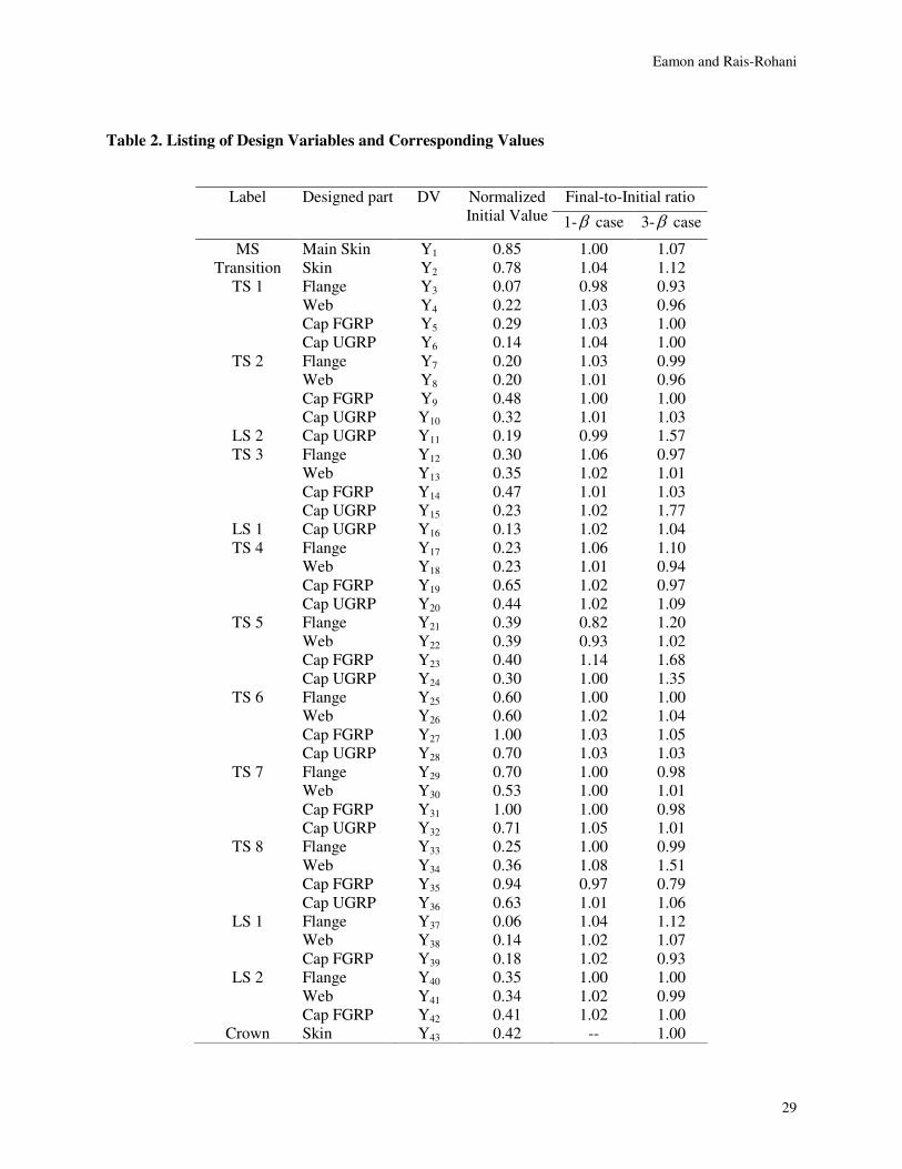
listing of design variables Y1 to Y43 is given in Table 2. The normalized initial values in Table 2

represent the normalized optimal values obtained through deterministic optimization of the CAS model

(Rais-Rohani et al. 2006). For the CAS RBDO problem, the lower and upper bounds for Y1 to Y42 are

taken as 0.5YkI and 2.0Yk

I, respectively, where Yk

I is the initial value of the kth design variable. For


10

Y43,the bounds are taken as Y43I

and 2.0Y43I

. The lower bounds represent the minimum thickness

necessary to satisfy other design constraints besides those considered in the RBDO problem.

The FE model of CAS as shown in Fig. 2 consists of approximately 18,600 four-node quadrilateral

and 350 three-node triangular shell elements paired with a material model that allows the discrete

modeling of individual layer properties. In addition to the outer surface, the webs, flanges, and caps of the

stiffeners are also discretely modeled as shell elements. The entire model has 96,700 degrees of freedom.

The base boundary of the CAS is constrained with a fixed boundary condition, representing its rigid

attachment to the submarine hull. The transient wave-slap, caused by an ocean wave striking the sail on

one side, is taken as the most critical load, and is modeled by an equivalent static load (uniform pressure)

on the port side of the sail (Cowan 2001). Both steel and GRP composite materials are modeled as linear

elastic. While the strength limit for the steel material is measured using von Mises criterion, that of GRP

is measured using the maximum strain based on the first-ply failure criterion of laminated composite

materials. Consequently, linear static FEA is used to determine the static strength of the structure while a

buckling eigenvalue solution is used to find its elastic stability.

Design Constraints in CAS RBDO

In order to identify the reliability-based and deterministic set of design constraints, a reliability

analysis of the deterministic-optimum CAS design was conducted with details presented in (Rais-Rohani

et al. 2006). However, for completeness sake, an overview of the selection process is described in this

section.

Reliability is measured in terms of component failure. There are 14 primary sail structural

components in the reliability model: the crown, main, transition, and base-joint skin along with ten

stiffeners. As noted above, most components are made of multiple GRP layers. Currently, no data are

available regarding material layer correlations. However, as described in Rais-Rohani et al. (2006), a

negligible difference in reliability was found between the fully correlated and uncorrelated material layer

models. Thus, full correlation among layer properties for a particular material type (FGRP, UGRP) within

a component is assumed, which greatly reduces computational effort from the uncorrelated case. For the


11

thin GRP plies making up the strain recovery layers (see Table 1), a separate limit state is formulated for

each strain component in the principal material directions. These limit states are expressed generically as

g1 = εtxmax−εtx (7)

g2 = εcxmax−εcx (8)

g3 = εtymax−εty (9)

g4 = εcymax−εcy (10)

g5 = γmax − γ (11)

where εtx and εcx are the axial tensile and compressive strains, respectively, in the fiber direction

whereas εty and εcy are the axial tensile and compressive strains, respectively, in the transverse direction,

with γ representing the in-plane shear strain. These strains are calculated from FEA of the CAS with

upper bounds equal to material allowable values. Limit states in Eqs. (7)-(11) apply to FGRP and UGRP

strain-recovery layers of the stiffeners as well as the FGRP strain-recovery layers in transition, main and

base joint regions of the skin. In addition, a limit on von Mises strain in the crown region and another on

buckling load factor of the whole structure brings the total number of potential limit states to 117.

The initial set of resistance random variables included four material stiffness parameters and five

material strength parameters with statistical properties described in Table 4. The GRP random variables

are the elastic moduli in the principal material directions (Exx, E

yy), shear modulus (G

xy), Poisson’s ratio

(νxy), the allowable tensile strains in each direction (εtxmax

,εtymax), the allowable compressive strains

(εcxmax,εcymax

), and the allowable in-plane shear strain (γmax ). For the steel crown, the random

variable is taken as the allowable von Mises strain, εst max. In addition, there is a load random variable, live

load pressure (LL). Based on the results of reliability analysis of GRP structures in a previous study

(Thompson et al. 2005), material thickness variability is deemed insignificant and not included here.

Separating all ±45°FGRP layers, all 0 /90° FGRP layers, all UGRP layers, and the steel parts regardless

of component into separate groups, and assuming each group has an independent set of material


12

properties, we find a total of 205 random variables in this system.

Although it is possible that some degree of correlation exists among the material property random

variables, no relevant data are yet available. Thus, they are currently assumed to be uncorrelated. Mean

maximum wave-slap load over the CAS design lifetime (30 years) is based on the available load data

while the corresponding coefficient of variation (COV) is based on an analysis of wave energy (Ozger et

al. 2004) found from ocean buoy data (NDBC 2005). All random variables are assumed to have a

normal probability distribution (Rais-Rohani et al. 2006).

The reliability analysis of the deterministic-optimum CAS model showed that the limit state on shear

strain of FGRP layers in transverse stiffeners (TS) generally had the lowest reliability index values, with

βTS5 = 1.84, βTS1 = 2.32, βTS7 = 3.29, βTS4 = 3.84, βTS2 = 3.98, and βTS6 = 4.05 representing the lowest six

beta values. Other low strength reliability indices were associated with von Mises strain in the crown

(CR) (βCR = 2.09), and axial tension strain of UGRP in TS7 (βTS7u = 3.97). As reference, a reliability

index of 2.33 translates into an approximate failure probability of 0.01 for the corresponding limit state.

The remaining material strength limit states, of the 116 total considered for the entire structure, had

substantially higher reliability indices ranging from 5.08 to greater than 10. Basing the reliability of the

CAS structural system on a first-component failure (series system) model, the few lowest component

reliability indices govern system performance.

The reliability index for the first buckling mode of the deterministic-optimum CAS design was found

to be 2.51. Using this value as the lowest acceptable component reliability index, the minimum reliability

indices of the lowest, most critical constraints are set equal to 2.51 while the remaining strength

constraints are treated as deterministic with bounds given in Table 3. Although buckling is an important

failure mode, it is not directly included in the RBDO due to its associated computational expense.

However, buckling performance is considered as part of the post-RBDO evaluation discussed later.

Hence, the critical set of limit states to be treated as reliability-based design constraints is reduced to

the following three


13

gγ = γmax − γFP (12)

gεt = εmax −εUP (13)

gcr = εstmax−εCR (14)

where gγ , gεt , and gcr represent the limit states for shear strain in FGRP plies of skin as well as cap, web,

and flange laminates of stiffeners, tensile strain in UGRP plies of stiffener caps, and von Mises strain in

the steel crown region, respectively, with strain bounds as those specified in Table 3. In Eqs. (12) - (14),

γmax,εmax, and εstmax represent the allowable maximum values for shear strain in FGRP plies, axial

strain in UGRP plies, and von Mises strain in steel, respectively. By examining the shear and axial strains

in all strain recovery layers that are made of FGRP or UGRP materials, we find the corresponding

maximum values denoted by γFP and εUP . For the steel crown, εCR represents the maximum von Mises

strain. The measured strain values are obtained from FE simulations as functions of material and loading

random variables.

The use of a single limit state for all layers throughout the structure that are made of the same

material is not meant to imply that full correlation exists among the component strengths. Rather, this is

the worst-case search approach in which reliability is calculated only for a component of a particular

material type (FGRP, UGRP, or steel) with the highest strain. These highest strain values become γFP ,

εUP , and εCR in the limit states gγ , gεt , and gcr , respectively. Since materials of the same type in all

components share the same statistical parameters for strength (regardless of correlation assumption), the

component with the highest load effect must necessarily have the lowest reliability index and is captured

in this process. Thus, for the CAS RBBO problem, a distinct evaluation of reliability for each individual

component is not needed, but rather only the minimum reliability index of any component is required.

The benefit of this approach is that it greatly reduces the number of probabilistic limit states (from 117 to

the three above), which is essential in managing the computationally intensive RBDO process.


14

In the CAS RBDO problem, both strength and stability requirements must be satisfied. For the

composite components, the strength requirements are formulated using the maximum-strain failure

criterion based on the first-ply failure theory of laminated composite materials. For each ply in the

laminate stack of a finite element, a separate upper bound is imposed on its tensile, compressive, and in-

plane shear strain values in principal material directions. With 19,880 elements having multiple GRP

layers, the number of strain constraints in the optimization problem could potentially reach as high as

several million. However, in the formulation and solution of the optimization problem only those

constraints that are active (i.e., g ≈ 0) or violated (i.e., g < 0) are used. Hence, the number of retained

constraints can be significantly less than the potential maximum and can vary from one optimization

cycle to another. As for structural stability, the load factor associated with the lowest buckling mode is

important in the CAS design.

The CAS RBDO problem is strictly one of structural optimization with sizing design variables.

Although other design considerations, such as hydrodynamic performance and manufacturing, can be

included in the optimization problem, they are not considered here.

Probabilistic Sensitivity Analysis

With the help of probabilistic sensitivity analysis, we can determine the influence of uncertainty

(represented by standard deviation) in each candidate random variable on the reliability index of selected

limit state functions. Hence, when the effect of uncertainty is important, the parameter is treated as

probabilistic; otherwise, it is treated as a deterministic parameter to reduce computational cost. The non-

dimensional probabilistic sensitivity derivative of a reliability index, β with respect to standard deviation

˜ σ X i of random variable, Xi can be calculated as (Madson, et al. 1986)

αi =∂β∂ ˜ σ X i

˜ σ Xi

β

(15)

From probabilistic sensitivity analysis of CAS model, we found that all of the material stiffness

random variables (i.e., Exx, E

yy, G

xy, and ν

xy) together with most of the strength random variables have


15

negligible effect on the selected strength-based limit states. Removing the insignificant random variables,

only four (i.e., LL, γmax,εmax, and εstmax) are necessary for inclusion in the CAS RBDO problem. Thus,

each of the three probabilistic limit states in Eqs. (13) – (15) is composed of only two random variables,

LL and the pertinent material ultimate strain value.

CAS RBDO Solution Procedure

The solution of CAS RBDO problem involves FEA of the CAS model for the evaluation of linear-

static responses of interest (i.e., strains), evaluation of reliability index associated with each probabilistic

design constraint, formulation and solution of an approximate optimization problem for updating the

values of design variables, and the evaluation of convergence criteria for termination of this iterative

process.

The mathematical programming techniques that are typically used to solve a nonlinear, constrained

optimization problem, such as the one defined by Eq. (6), require gradients of the objective function and

those of the retained design constraints with respect to each design variable. When the objective function

and/or constraints are implicit functions of design variables, as is the case here, the sensitivity derivatives

are commonly calculated using a finite difference scheme, which can significantly increase the

computational cost.

The constrained optimization problem is solved using the Modified Method of Feasible Directions

(MMFD) in the VisualDOC (2002) program. MSC/NASTRAN (2001) is used as the FEA solver, and the

probabilistic code NESSUS (2001), which contains the AMV+ method, is used to calculate the reliability

indices. The communication among the individual codes is organized and managed using the

VisualScript (2002) program. Additionally, several in-house FORTRAN codes are used to facilitate the

recording of appropriate analysis input and output files and searching for and extracting critical responses.

A flowchart of the general steps in a single CAS RBDO cycle is given in Figure 3. A cycle starts

with the optimizer determining trial values for the design variables (DVs). Note that in the very first

cycle, the initial values of design variables are used. An FEA is performed and the deterministic


16

constraints are evaluated. With design variables held fixed, the random variables (RVs) are perturbed and

the model is analyzed for reliability. The random-variable perturbations are continued until the reliability

index calculation for each probabilistic constraint is completed. Based on the gradient information from

the objective and constraint functions, the MMFD algorithm establishes a usable-feasible search direction

to find an improved design point. The optimizer checks the optimality and convergence criteria at that

point, and if necessary, additional optimization cycles are performed until an optimum solution is found.

CAS RBDO Results

For comparison purposes, we considered two different RBDO cases. In the 3-β case, the RBDO

problem, as described above, consists of 43 design variables, 8 deterministic constraints, and 3 reliability-

based constraints whereas in the 1-β case, a less computationally expensive problem with 42 design

variables, 10 deterministic constraints, and only one reliability-based constraint (see Table 3) is solved.

In the 1-β case, crown thickness is held fixed and two of the probabilistic constraints (βεt and βcr) are

taken as deterministic (i.e., converted to εtx for UGRP and εst in Table 3, respectively) while the FGRP

shear strain constraint, βγ , which initially had the lowest component reliability index of 1.84, is taken as

probabilistic.

3- β β β β CASE

The deterministic-optimum CAS model (Rais-Rohani et al. 2006) with a weight of 75,430 lb is

chosen at the initial design for the RBDO problem. The RBDO problem required 170 CPU hours on a

SUN Sparc workstation to converge in 7 cycles to an optimal design having a weight of 79,360 lb,

representing a weight increase of 5%. The weight increase is due to the selected value of βmin = 2.51,

which is higher than the level of reliability in the initial design. The only way the optimizer was able to

satisfy the higher reliability level was by increasing the wall thickness, hence the higher weight. The

effect that the increase in reliability has on component and system safety is discussed below. The

convergence history of the objective function is shown in Figure 4.


17

Final design variable values, as a fraction of the original, are given in Table 2. Most plies were only

mildly affected and had less than 5% change in thickness. This is because the initial design variable

values were based on deterministically optimized problem. Thus, many of the design variables, which

were primarily governed by the large number of deterministic constraints in the model, were close to their

optimal values before the start of the RBDO process. Significant thickness gains occurred in the main

skin (7%); the transition region (12%); TS4 flange (10%); LS1 flange (12%); TS5 flange (20%), cap

FGRP (68%) and cap UGRP (35%); TS8 web (51%); LS2 cap UGRP (57%); and TS3 cap UGRP (77%).

Although individual members experienced a minor (between 1-7%) loss of weight except TS5 and TS6,

the total weight saving was more significant. The TS8 cap FGRP material loss was 21%. Losses were

fairly evenly distributed among stiffener webs, caps, and flanges, but only the FGRP material was

affected. Final constraint response values as well as the critical component locations are given in Table

3. As seen in the “Final-to-Bound Ratio” and “Critical Component” columns for the 3-β case, the most

critical constraints in the post-RBDO CAS were εcx for FGRP in the transition region and βcr (with final

value = 2.51).

An interesting result can be seen in the change in design variable values, which also illustrates the

difficulty in choosing optimum solutions for complex structures without rigorous mathematical guidance.

At the initial design, three components had a reliability index below the imposed limit of 2.51. These

included the FGRP material of TS1 and TS5 that was shear-limited (βTS5 = 1.84; βTS1 = 2.32) and the

crown (βcr=2.09). Although the component with the lowest initial reliability index, TS5, made significant

gains in ply thickness as expected, the crown, with the next lowest reliability index, had no significant

difference in material thickness. Finally, TS1, the final component with an initial reliability index less

than that required, experienced a net loss of material. Apparently, the best solution to meet the minimum

β constraints and yet minimize weight was to globally stiffen the structure by increasing thickness of the

outer shell as well as the most significant stiffeners in this regard (i.e., TS3-5, and LS1-2). This makes

sense particularly with regard to the crown, which is a large volume of material (controlled by a single


18

design variable) as well as relatively heavy (steel) material as compared to the lightweight composite

material used elsewhere in the CAS structure.

The importance of global stiffness can also be seen in the sensitivity analysis. Normalized

sensitivities of the objective function and constraints with respect to design variables are presented in

Figures 5 to 8.

Figure 5 presents the sensitivities of the objective function. Clearly, the main skin thickness (Y1) is

the most critical design variable, as this represents the component with the most volume of material. In

Figure 5, sensitivities are identical for the initial and optimal design models, as expected.

In Figures 6 to 8, only the design variables that significantly impact the constraint are presented.

Positive values indicate that an increase in layer thickness increases the response while negative values

indicate increasing thickness decreases the response. In general, the main skin (Y1) has a strong influence

on almost every constraint. Also important for most constraints is the transition region (Y2), and the

FGRP and UGRP cap material in TS5 (Y23 and Y24, respectively). Stiffener components that appear most

frequently on the graphs are TS5, TS4, and TS8. Also appearing, but less frequently, are TS3, TS7, and

LS2. The remaining stiffeners are insignificant with respect to constraint sensitivity. Among the

stiffeners, the cap material is most critical for most constraints, with the flange material least important.

Figure 8 presents the probabilistic constraints. As the constraints βεt and βcr became inactive during the

RBDO, only their initial sensitivity values are presented. For the most part, initial and optimum

sensitivity values are similar.

Note that there is often no obvious link between the critical component in Table 3 and the most

important design variable affecting the strain responses in that component as indicated by the sensitivity

plots. For example, in Table 3, consider the εty response in the UGRP layer for the 1-β case. Here an

element in TS7 was found to govern the constraint εty. Referring to Figure 6, this constraint was found to

be most sensitive to design variables numbered 1, 11, and 32. Of these three, only one, Y32 appears in

component TS7 (see Table 2), while the two most influential design variables, Y1 and Y11, appear in the

main skin and in longitudinal stiffener LS2, respectively. Similar results can be seen for the other


19

constraints as well. The reason for this somewhat non-intuitive result, as discussed above, is that a design

variable with significant influence on the overall structural stiffness is generally a better indicator of

importance than one that corresponds to the critical component thickness itself. For example, increasing

the design variable value corresponding to critical component thickness increases strength but also local

stiffness, and thus attracts more force to that component, resulting in strain remaining relatively constant

(and thus the sensitivity of the strain limit constraint to that design variable remains low) as compared to

adjusting shell thickness everywhere, which more rapidly minimizes strain in all of the stiffeners.

1-ββββ CASE

The 1-β case required approximately 50 CPU hours to converge in six cycles (Figure 4) to a new

mass of 75,600 lb, representing an increase of approximately 0.4%. The lower final mass value as

compared to the 3-β case is because the probabilistic crown constraint βcr was not imposed in this case.

Therefore, as the initial and final maximum crown strains are identical, as indicated in the “Final-to-Initial

Ratio” column in Table 3, the crown reliability index would remain at the initial value of 2.09 (as opposed

to 2.51 in the 3-β case). Final design variable values are given in Table 2. Most plies were only mildly

affected and had less than 3% change in thickness.

As indicated in Table 2, plies that lost thickness were the FGRP plies in the flanges of TS1 (2% loss)

and TS5 (18%). The cap material of TS8 (3%) and LS2 (1%), and the web of TS5 (7%) also experienced

reductions in thickness. Plies with relatively large gains in thickness are the flange plies of TS3 and TS4

(both 6% increase), the FGRP plies in the cap of TS5 (14%) and the web of TS8 (8%). As shown in

Table 3, the probabilistic FGRP shear constraint (βγ) and the deterministic crown strain constraint, εcr

were most critical, with both responses equal to the bound values. The 1-β case sensitivities are very

similar to those of the 3-β case and are not presented here.

System Reliability Analysis

The CAS is a structural system composed of various components, and the reliability of this system

may be altered during the optimization process. To estimate the system reliability of CAS-RBDO model,


20

the procedure in Rais-Rohani et al. (2006) is used. A total of 116 limit states corresponding to 14 primary

structural components are considered for the structure as described in Table 5. Separating FGRP and

UGRP materials in each stiffener and treating them as independent sub-components, produces a reliability

model with total of 24 components. For members that are made of GRP materials, component failure is

characterized by the violation (g<0) of any of the limit states as described in Eqs. (7) – (11). For the steel

crown, a single limit state, yield (as determined by von Mises stress), is considered in place of limit states

g1 to g5.

The probability of failure of the series system of n uncorrelated components (ρ = 0) for limit state j,

Pfj, is given by

Pfj =1− 1− Pfji( )i=1

n

∏ (16)

where Pfji is the failure probability of component i considering limit state j. If the components are fully

correlated (ρ = 1), Pfj, is given by

Pfj =max(Pfji ) (17)

When the degree of correlation is uncertain, as is the case here, a failure probability bounds can be

constructed by considering both Eqs. (16) and (17), which represent upper and lower bounds,

respectively. If the resulting bounds are not too wide, the results may be acceptable and the exact

correlation is not needed. If the difference between the bounds is unacceptably large, a more

computationally costly method may be required for a more accurate solution. Using Eqs. (16) and (17),

there is a need to compute Pf for each component. This is governed by the finite element with the highest

load effect within the component. The AMV+ method, as described above, is used for reliability analysis.

As noted, detailed component and limit-state specific results for the pre-RBDO CAS reliability

analysis are given elsewhere (Eamon and Rais-Rohani 2008), and a complete re-computation of


21

individual component reliability considering each of the 116 limit states is beyond the scope of this study.

However, some meaningful results can be obtained using some simplifying assumptions.

Considering the Final-to-Initial Ratio column for the 1-β case in Table 3, we find that all

deterministic critical responses except that for shear strain (γ) in the UGRP were slightly below their

respective initial values. Thus, reliability indices for all limit states except UGRP γ will be above initial

values. For UGRP γ, the initial reliability index was very high (13.2), and lowering this reliability index

by a large amount (greater than 50%) will have no impact on CAS system reliability, which is governed

by indices much lower. Therefore, the decrease in reliability index associated with the small increase in

response value for UGRP γ is of no consequence for system results. A similar situation exists for the 3- β

case, where two additional post-RBDO critical responses were slightly higher than the initial values ( txε

and cxε for FGRP). However, these initial reliability indices were also much higher than those governing

CAS reliability, and thus even large decreases in reliability for these responses will not affect system

results. Given these observations, post-RBDO system reliability can be conservatively estimated using

Eqs. (16) and (17) by assuming all previous component reliabilities (calculated using the limit states g1 to

g5) remain unchanged from those of the pre-RBDO CAS, with the exception of those affected (i.e.,

increased) by the three imposed probabilistic constraints (βγ, βεt, and βcr) with post-RBDO values given in

Table 3.

A final important limit state to note is buckling. Evaluated with an FEA Euler analysis, no direct link

can be obtained for buckling resistance and a single CAS component, as eigenvalues are computed for the

structural system as a whole. However, as buckling anywhere in the structure is taken as failure and

multiple buckling locations are possible, a series sub-system model can be developed such that each

buckling mode constitutes a ‘component’. Both fully-correlated and uncorrelated bounds can be

developed for the buckling sub-system using Eqs. (16) and (17). The higher modes that do not

significantly contribute to Pf may be truncated. It was found that no more than five modes need be


22

considered. Buckling load factors (eigenvalues) for the pre- and post-RBDO CAS are given in Table 6.

Note that in all cases, post-RBDO buckling load factors are higher.

Using the simplifications described above, the series system reliability results are given in Table 7.

Considering the entire structure with all limit states including buckling, the deterministic optimum (pre-

RBDO) CAS has reliability index bounds between 1.46 and 1.84. For the 1-β case, system reliability

bounds are between 1.74 and 2.09, while for the 3-β case, system bounds are between 2.10 and 2.33.

Using the standard normal conversion from reliability index to failure probability, Pf = Φ(−β) in the 1-β

case, for a 0.4% increase in mass, the decrease in system failure probability is approximately 50% (pre-

RBDO: 0.034 < Pf < 0.071; RBDO (1- β): 0.018 < Pf < 0.042). In the 3-β case, for a 5% increase in mass,

the decrease in failure probability is approximately 70% (RBDO (3- β): 0.010 < Pf < 0.018). Of course,

larger gains in reliability can be achieved by increasing the target probabilistic constraint values, at the

expense of larger increases in structural mass.

Conclusion

In this paper, we presented the description of RBDO methodology and its application in design of a large

and complex marine structural system under uncertainties in load intensity and material resistance

characteristics. The design procedure required the direct coupling of finite element analysis, numerical

design optimization, and structural reliability algorithms while considering different modes of failure in

the stiffened shell structure made of both metallic and laminated GRP composite materials. Through

probabilistic sensitivity analysis, critical random variables were identified. The RBDO solutions indicated

that a minor increase in structural mass can significantly increase both the component and system

reliabilities of the CAS structure. Moreover, the overall structural stiffness was found to be generally

more significant than critical component thickness values..

The inclusion of reliability-based design constraints was found to be the most expensive part of the

algorithm, where moving from one to three such constraints more than tripled the computational cost (50

CPU hours to 170 CPU hours). Thus, judicial use of the number of reliability constraints, as was done in


23

this study, is essential to maintain reasonable computational effort when confronted with complex

reliability-based structural optimization problems.


24

APPENDIX: Nomenclature

a constant in objective function

ν Poisson ratio

AMV+ advanced mean value plus method

CAS Composite Advanced Sail

CR crown

cx compression, x-direction

cy compression, y-direction

d composite layer that has thickness as a DV

DV design variable

E modulus of elasticity

FEA finite element analysis

FGRP fabric GRP

FP critical FGRP strain

fx probability density function

g limit state function

G shear modulus

GRP glass-reinforced polymer

hst steel plate layer of base joint

LL wave slap load random variable

MMFD Modified Method of Feasible Directions

MPP most probable point of failure

Pf probability of failure

R response

RBDO reliability-based design optimization

RV random variable

t composite layer used for strain recovery

TS transverse stiffener

tx tension, x-direction

ty tension, y-direction

UGRP uni-directional GRP

UP critical UGRP strain

X a random variable

x* RV values at MPP

Y a design variable

z standard normal (reduced) RV

α probabilistic sensitivity

β reliability index

γ shear strain

ε strain

µ mean value

σ standard deviation

Ф standard normal cumulative distribution function


25

REFERENCES

Brown, P. W., Jordaan, I. J., Nessim, M. A., Haddara, M.R., “Optimization of Bow Plating for

Icebreakers,” Journal of Ship Research, Vol. 40, No. 1, 1996, pp. 70-78.

Cowan, A.L., “AS98T Global Analysis Summary (FY 01),” Naval Surface Warfare Center, Carderock

Division, CASP-01-011, Oct 2001.

Du, X. and Chen, W., “Sequential Optimization and Reliability Assessment Method for Efficient

Probabilistic Design,” Journal of Mechanical Design, Vol. 126, No. 2, 2004, pp. 225-233.

Eamon, C. and Rais-Rohani, M., “Structural Reliability Analysis of Advanced Composite Sail,”

SNAME Journal of Ship Research (to appear June, 2008).

Eamon, C., Thompson, M., and Liu, Z., “Evaluation of Accuracy and Efficiency of some Simulation and

Sampling Methods in Structural Reliability Analysis,” Structural Safety, Vol. 27, No. 4, 2005, pp. 356-

392.

Enevoldsen, I. and Sorensen, J. D., “Reliability-Based Optimization in Structural Engineering,”

Structural Safety, Vol. 15, 1994, pp. 169-196.

Frangopol, D. M., “Reliability-Based Optimum Structural Design,” Probabilistic Structural Mechanics

Handbook, Theory and Industrial Applications, edited by Sundararajan, C., Chapman & Hall, 1995.

Jang, C.D., Kim, H.K., and Song, H.C., “Optimum Structural Design of High-Speed Surface Effect Ships

Built of Composite Materials,” Marine Technology, Vol. 40, 2003, pp. 42-48.

Leheta, H. W. and Mansour, A. E., “Reliability-based method for optimal structural design of stiffened

panels,” Marine Structures, Vol. 10, No. 5, 1997, pp. 323-352.

Madson, H. O., Krenk, S., and Lind, N. C., Methods of Structural Safety, Prentice-Hall, Inc., New Jersey,

1986, pp. 120-123.

MSC/NASTRAN Quick Reference Guide (v 2001). (2001). MacNeal-Schwendler Corp., Los Angeles,

CA, U.S.

Morandi, A.C., Das, P.K., and Faulkner, D., “An Outline of the Application of Reliability Based

Techniques to Structural Design and Assessment of Submarines and Other Externally Pressurized

Cylindrical Structures,” Marine Structures, Vol. 7, 1994, pp. 173-187.

National Data Buoy Center website. www.ndbc.noaa.gov. 2005

NESSUS Theoretical Manual. October 2001, Southwest Research Institute, San Antonio, TX.

Ozger, M, Altunkaynak, A., and Sen, Z., “Statistical Investigation of Wave Energy and its

Reliability,” Energy Conversion and Management, Vol. 45, 2004, pp. 2173-2185.

Pu, Y., Das, P.K., Faulkner, D. “Strategy for reliability-based optimization,” Engineering Structures,

Vol. 19, No. 3, 1997, pp. 276-282.

Qu, X. and Haftka, R. T., “Reliability-Based Design Optimization Using Probabilistic Safety Factor,”

Structural and Multidisciplinary Optimization, Vol. 27, No. 5, 2004, pp. 314-325.


26

Rackwitz, R. and Fiessler, B. “Structural Reliability Under Combined Random Load Sequence,”

Computers and Structures, No. 9, 1978.

Rais-Rohani, M., Eamon, C., and Keesecker, A., “Structural Analysis and Sizing Optimization of

a Composite Advanced Sail Design Concept,” Marine Technology, Vol. 42,

No. 2, 2005, pp 61-70.

Rais-Rohani, M., Eamon, C., Lokits, J., Telegadas, H., and Bonanni, D., “Structural Analysis and

Optimization of Composite Advanced Sail Design Concepts for Virginia-Class Submarines,” NSWCCD-

65-TR-2006/01, Naval Surface Warfare Center Carderock Division, Jan 2006.

Rais-Rohani, M. and Lokits, J., “Reinforcement Layout and Sizing Optimization of Composite Submarine

Sail Structures,” Structural and Multidisciplinary Optimization, Vol. 34, No. 1, 2007, pp. 75-90.

Rao, S.S., Reliability-Based Design, McGraw-Hill, Inc., 1992.

Rao, S.S., Engineering Optimization Theory and Practice, 3rd Ed., John Wiley & Sons, Inc., 1996.

Sprecace, A., “Parametric Analyses of Stiffening Arrangements for the ATSOL 12 Advanced Sail,”

Naval Surface Warfare Center Carderock Division, Contract Rept. CASP-01-01, 2000.

Thompson, M., Eamon, C., and Rais-Rohani, M., “Reliability-Based Optimization of Composite

Bridge Decks,” ASCE Journal of Structural Engineering, Vol. 132, No. 12, 2006, pp. 1898-1906.

Tu, J., Choi, K. K., and Park, Y. H., “A New Study on Reliability Based Design Optimization,” Journal

of Mechanical Design, Vol. 121, No. 4, 1999, pp. 557–564.

Wu, Y.-T., Millwater, H. R., and Cruse, T. A., “An Advanced Probabilistic Structural Analysis Method

for Implicit Performance Functions,” AIAA Journal, Vol. 28, No. 9, 1990, pp. 1840-1845.


27

List of Tables

Table 1. Material systems for the skin and stiffeners in CAS finite element model

Table 2. Design Variables

Table 3. Design Constraints

Table 4. Random Variable Statistical Parameters

Table 5. Components and Limit States

Table 6. Buckling Load Factors

Table 7. Estimated System Reliability Indices

List of Figures

Figure 1. Conceptual Model of the CAS.

Figure 2. Finite Element Model of the CAS with Highlighted Stiffener Layout

Figure 3. RBDO Flowchart

Figure 4. Convergence History

Figure 5. Normalized sensitivities of sail weight with respect to design variables.

Figure 6. Normalized sensitivities of deterministic UGRP constraints with respect to significant

design variables.

Figure 7. Normalized sensitivities of deterministic FGRP constraints with respect to significant

design variables.

Figure 8. Normalized sensitivities of probabilistic constraints with respect to significant design

variables.


28

Table 1. Material systems for the skin and stiffeners in CAS finite element model

Structural Part Material System Laminate Composition Thickness

Crown Steel Single Layer dC

Transition FGRP [0-90/0-90/±45/±45/0-90]S [t/dT/t/dT/t]s

Main FGRP [0-90/0-90/±45/±45/0-90]S [t/dM/t/dM/t]s

Base Joint Steel/FGRP/Steel [ST/0-90/0-90/±45/±45/0-

90/0-90/±45/±45/0-90/0-

90/ST]

[hst1/t/dB/t/dB/t/t/dB/t/dB/t/hst2]

Stiffener Flange FGRP [±45/±45/±45/±45/±45]S [t/df/t/df/t]s

Stiffener Web FGRP [±45/±45/±45/±45/±45]S [t/dw/t/dw/t]s

Stiffener Cap FGRP & UGRP [±45/±45/0/0/±45/±45/±45]S [t/dc1/t/dc2/t/dc1/t]s


29

Table 2. Listing of Design Variables and Corresponding Values

Final-to-Initial ratio Label Designed part DV Normalized

Initial Value 1-β case 3-β case

MS Main Skin Y1 0.85 1.00 1.07

Transition Skin Y2 0.78 1.04 1.12

TS 1 Flange Y3 0.07 0.98 0.93

Web Y4 0.22 1.03 0.96

Cap FGRP Y5 0.29 1.03 1.00

Cap UGRP Y6 0.14 1.04 1.00

TS 2 Flange Y7 0.20 1.03 0.99

Web Y8 0.20 1.01 0.96

Cap FGRP Y9 0.48 1.00 1.00

Cap UGRP Y10 0.32 1.01 1.03

LS 2 Cap UGRP Y11 0.19 0.99 1.57

TS 3 Flange Y12 0.30 1.06 0.97

Web Y13 0.35 1.02 1.01

Cap FGRP Y14 0.47 1.01 1.03

Cap UGRP Y15 0.23 1.02 1.77

LS 1 Cap UGRP Y16 0.13 1.02 1.04

TS 4 Flange Y17 0.23 1.06 1.10

Web Y18 0.23 1.01 0.94

Cap FGRP Y19 0.65 1.02 0.97

Cap UGRP Y20 0.44 1.02 1.09

TS 5 Flange Y21 0.39 0.82 1.20

Web Y22 0.39 0.93 1.02

Cap FGRP Y23 0.40 1.14 1.68

Cap UGRP Y24 0.30 1.00 1.35

TS 6 Flange Y25 0.60 1.00 1.00

Web Y26 0.60 1.02 1.04

Cap FGRP Y27 1.00 1.03 1.05

Cap UGRP Y28 0.70 1.03 1.03

TS 7 Flange Y29 0.70 1.00 0.98

Web Y30 0.53 1.00 1.01

Cap FGRP Y31 1.00 1.00 0.98

Cap UGRP Y32 0.71 1.05 1.01

TS 8 Flange Y33 0.25 1.00 0.99

Web Y34 0.36 1.08 1.51

Cap FGRP Y35 0.94 0.97 0.79

Cap UGRP Y36 0.63 1.01 1.06

LS 1 Flange Y37 0.06 1.04 1.12

Web Y38 0.14 1.02 1.07

Cap FGRP Y39 0.18 1.02 0.93

LS 2 Flange Y40 0.35 1.00 1.00

Web Y41 0.34 1.02 0.99

Cap FGRP Y42 0.41 1.02 1.00

Crown Skin Y43 0.42 -- 1.00


30

Table 3. Listing of Properties Treated as Design Constraints

Deterministic Constraints

RBDO (3-β)* RBDO (1-β)* Property Lower

Bound

Upper

Bound

Initial

Value Final-

to-

Bound

Ratio

Final-

to-

Initial

Ratio

Critical

Comp.

Final-

to-

Bound

Ratio

Final-

to-

Initial

Ratio

Critical

Comp.

UGRP (in stiffener caps)

εtx none 0.00685 0.0066 -- -- -- 0.94 0.98 TS7

εty none 0.00685 0.0055 0.71 0.89 TS6 0.79 0.98 TS7

εcx -0.0057 none -0.0049 0.79 0.90 TS4 0.86 0.99 TS4

εcy -0.0057 none -0.0040 0.61 0.88 TS1 0.69 0.99 TS2

γ -0.0114 0.0114 0.0041 0. 33 1.12 TS8 0.37 1.02 TS8

FGRP (in skin and stiffeners)

εtx none 0.00685 0.0060

(0.0048)

0.94

(0.57)

1.06

(0.81)

transition

(TS4)

0.87

(0.70)

0.99

(0.99)

main skin

(TS3)

εty none 0.00685 0.0057

(0.0048)

0.74

(0.66)

0.88

(0.94)

main skin

(TS4)

0.83

(0.69)

0.99

(0.99)

main skin

(TS4)

εcx -0.00587 none -0.0058

(-0.0056)

1.00

(0.79)

1.04

(0.92)

transition

(TS3)

0.98

(0.91)

0.95

(0.98)

main skin

(TS8)

εcy -0.00587 none -0.0056

(-0.0051)

0.91

(0.79)

1.00

(0.85)

main skin

(TS3)

0.95

(0.85)

0.97

(0.99)

main skin

(TS3)

Steel (Crown)

εst none 0.00210 0.00210 -- -- -- 1.00 1.00 crown

Probabilistic Constraints

RBDO (3-β) RBDO (1-β) Property Lower

Bound

Upper

Bound

Initial

Value Final Value Critical Comp. Final Value Critical Comp.

βγ 2.51 none 1.84 3.20 TS5 2.51 TS5

βεt 2.51 none 3.97 4.19 TS7 -- --

βcr 2.51 none 2.09 2.51 crown -- --

*Numbers in parentheses refer to results considering components 1-10 (i.e. the stiffeners) only while the

upper number (without parentheses) considers results from all components including crown, main skin,

and transition region.


31

Table 4. Statistical Properties of Random Variables

FGRP UGRP

RV mean COV distribution mean COV distribution

Exx* 3.50e6 psi 0.055 normal 5.53e6 psi 0.055 normal

Eyy* 3.50e6 psi 0.055 normal 1.42e6 psi 0.055 normal

Gxy* 5.0e5 psi 0.003 normal 5.0e5 psi 0.003 normal

νxy* 0.098901 0.003 normal 0.2424 0.003 normal

εtxmax or εtymax 0.0138 0.065 normal 0.012 0.065 normal

εcxmax or εcymax -0.0121 0.050 normal -0.010 0.050 normal

γmax 0.015 0.015 normal 0.015 0.015 normal

Other

LL λ=2.28** 0.167 normal

Est max* 2.96e6 psi 0.01 normal

νst* 0.30 0.026 normal

εstmax 0.00290 0.05 lognormal

*These RVs were found to be insignificant in the probabilistic sensitivity analysis and hence were excluded in the

RBDO solutions.

**Bias factor (ratio of mean to nominal) is given. Load magnitude is comparable to hurricane-level wind pressure,

but exact value is not available for public release.

Table 5. Components and Limit States

Comp

#

Component

Name

Material Sub-

Components

Limit States

Considered

Total # of Limit

States per

Component

1-10 Stiffener 1-10 FGRP, UGRP g1-g5, g1-g5 10 (x 10 stiffeners)

11 Transition FGRP g1-g5 5

12 Main Skin FGRP g1-g5 5

13 Crown Steel yield 1

14 Base Joint FGRP g1-g5 5

Total # of Limit States: 116


32

Table 6. Buckling Load Factors for Different CAS Designs

Mode Pre-RBDO RBDO (1-β) RBDO (3-β) 1 1.42 1.45 1.72

2 1.44 1.49 1.77

3 1.55 1.60 1.79

4 1.67 1.67 1.85

5 1.77 1.84 1.87

Table 7. Estimated System Reliability Indices

Subsystem Pre-RBDO RBDO (1-β) RBDO (3-β) Considered in CAS β, ρ = 0 β, ρ = 1 β, ρ = 0 β, ρ = 1 β, ρ = 0 β, ρ = 1

all components 1-14 (g1-g5) 1.54 1.84 1.80 2.09 2.10 2.33

buckling 2.29 2.52 2.55 2.69 4.23 4.31

all components + buckling 1.46 1.84 1.74 2.09 2.10 2.33


33

Figure 2. Finite element model of the CAS with highlighted stiffener layout

Artist rendering of a VA-Class

submarine with CAS

Figure 1. Conceptual model of the CAS.

Main

Base Joint

Crown

Transition

LS1

LS2

TS1 TS2 TS3 TS4 TS5 TS6 TS7 TS8


34

Figure 3. CAS RBDO flowchart


35

150

160

170

180

190

200

210

220

230

240

250

1 2 3 4 5 6 7 8

Optimization Cycle

Sa

il M

as

s (

lbs

/38

6 in

/s^

2)

3 β case

1 β case

Figure 4. Convergence history

Objective Function

0.00

0.10

0.20

0.30

0.40

0.50

0.60

0.70

0.80

0.90

1.00

1 3 5 7 9 11 13 15 17 19 21 23 25 27 29 31 33 35 37 39 41 43

Design Variable No.

Sen

sit

ivit

y

Figure 5. Normalized sensitivities of CAS weight with respect to design variables.


36

Figure 6. Normalized sensitivities of deterministic UGRP constraints with respect to significant

design variables.

Figure 7. Normalized sensitivities of deterministic FGRP constraints with respect to significant

design variables.


37

Figure 8. Normalized sensitivities of probabilistic constraints with respect to significant design

variables.

integrated reliability and sizing optimization of a large

Documents