instrumentation and analysis of a perpetual pavement on … pavement in oregon... ·...
TRANSCRIPT

Instrumentation and Analysis of a Perpetual Pavement on an Interstate Freeway in Oregon Authors: Todd V. Scholz, P.E., Assistant Professor (Corresponding) Department of Civil, Construction, and Environmental Engineering 220 Owen Hall Oregon State University Corvallis, Oregon 97331 Phone: 541.737.2056 Fax: 541.737.3300 Email: [email protected]
Jim Huddleston, P.E., Executive Director Asphalt Pavement Association of Oregon 5240 Gaffin Road SE Salem, Oregon 97301 Phone: 503.363.3858 Fax: 503.363.5571 Email: [email protected] Elizabeth A. Hunt, P.E., Pavement Services Engineer Construction Section, Oregon Department of Transportation 800 Airport Road SE Salem, Oregon 97301 Phone: 503.986.3115 Fax: 503.986.3096 Email: [email protected] James R. Lundy, P.E., Associate Dean College of Engineering 101 Covell Hall Oregon State University Corvallis, Oregon 97331 Phone: 541.737.5235 Fax: 541.737.1805 Email: [email protected] Norris C. Shippen, Research Coordinator Planning Section, Oregon Department of Transportation 200 Hawthorne SE, Suite B-240 Salem, Oregon 97301 Phone: 503.986.3538 Fax: 503.986.2844 Email: [email protected]
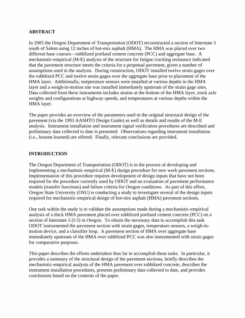
ABSTRACT In 2005 the Oregon Department of Transportation (ODOT) reconstructed a section of Interstate 5 south of Salem using 12 inches of hot-mix asphalt (HMA). The HMA was placed over two different base courses—rubblized portland cement concrete (PCC) and aggregate base. A mechanistic-empirical (M-E) analysis of the structure for fatigue cracking resistance indicated that the pavement structure meets the criteria for a perpetual pavement, given a number of assumptions used in the analysis. During construction, ODOT installed twelve strain gages over the rubblized PCC and twelve strain gages over the aggregate base prior to placement of the HMA layer. Additionally, temperature sensors were installed at various depths in the HMA layer and a weigh-in-motion site was installed immediately upstream of the strain gage sites. Data collected from these instruments includes strains at the bottom of the HMA layer, truck axle weights and configurations at highway speeds, and temperatures at various depths within the HMA layer. The paper provides an overview of the parameters used in the original structural design of the pavement (via the 1993 AASHTO Design Guide) as well as details and results of the M-E analysis. Instrument installation and instrument signal verification procedures are described and preliminary data collected to date is presented. Observations regarding instrument installation (i.e., lessons learned) are offered. Finally, relevant conclusions are provided. INTRODUCTION The Oregon Department of Transportation (ODOT) is in the process of developing and implementing a mechanistic-empirical (M-E) design procedure for new work pavement sections. Implementation of this procedure requires development of design inputs that have not been required for the procedure currently used by ODOT and an evaluation of pavement performance models (transfer functions) and failure criteria for Oregon conditions. As part of this effort, Oregon State University (OSU) is conducting a study to investigate several of the design inputs required for mechanistic-empirical design of hot-mix asphalt (HMA) pavement sections. One task within the study is to validate the assumptions made during a mechanistic-empirical analysis of a thick HMA pavement placed over rubblized portland cement concrete (PCC) on a section of Interstate 5 (I-5) in Oregon. To obtain the necessary data to accomplish this task ODOT instrumented the pavement section with strain gages, temperature sensors, a weigh-in-motion device, and a classifier loop. A pavement section of HMA over aggregate base immediately upstream of the HMA over rubblized PCC was also instrumented with strain gages for comparative purposes. This paper describes the efforts undertaken thus far to accomplish these tasks. In particular, it provides a summary of the structural design of the pavement sections, briefly describes the mechanistic-empirical analysis of the HMA pavement over rubblized concrete, describes the instrument installation procedures, presents preliminary data collected to date, and provides conclusions based on the contents of the paper.

PROJECT LOCATION The project is located on Interstate 5 just north of Albany as indicated in Figure 1. This part of the interstate is in the Willamette Valley which is bordered by the Coast Mountain Range to the West and Cascade Mountain Range to the East. The instrumented portion of the project is located in the southbound lanes which carry significantly higher truck traffic as compared with the northbound lanes.
Project Location
Project Location
FIGURE 1 Project Location.
STRUCTURAL DESIGN The existing southbound mainline pavement was constructed in 1958 using 8 inches (200 mm) of jointed reinforced concrete pavement (JRCP) over aggregate base that ranged from 9 to 12 inches (225 to 300 mm) in thickness depending on location. Subsequent to the original construction, the section had received a 6 inch (150 mm) HMA overlay in 1990 or 1991. Overall the pavement was in fair condition except in areas where the HMA overlay was thinned down to meet grade under structures. In these areas joint faulting in the underlying JRCP was evident and the HMA overlay exhibited extensive reflection cracking over the joints in the JRCP as well as raveling and potholes. ODOT considered several rehabilitation and reconstruction alternatives. These included:
1. Overlay the existing pavement with HMA 2. Complete reconstruction using HMA 3. Complete reconstruction using continuously reinforced concrete pavement (CRCP) 4. Remove the HMA layer, rubblize the JRCP, and overlay with HMA 5. Remove the HMA layer, rubblize the JRCP, and overlay with CRCP

Life cycle cost analyses indicated that long-term maintenance costs associated with the first alternative and initial construction costs associated with the second and third alternatives made all three of these alternatives unattractive relative to the fourth and fifth options. The analyses also indicated that long-term costs associated with the fourth and fifth alternatives to be essentially equal. The fourth alternative was ultimately selected because it could be constructed faster for lower initial cost and would be easier and cheaper to maintain over the long term with periodic surface milling and repaving. However, the second alternative was used in short sections to meet clearance requirements under structures. Thus, two structural sections were developed. ODOT used the National Asphalt Pavement Association (NAPA) guide for HMA overlays on PCC pavements (1) for the structural section incorporating the rubblized JRCP, which has been recently superseded by NAPA’s guide for rubblization (2). The guide provides a procedure based on the American Association of State Highway and Transportation Officials (AASHTO) structural deficiency approach (3) to determine the required thickness of an HMA overlay placed over fractured concrete pavements. The designer used the Level I and Level II approaches with uncorrected and corrected subgrade soil moduli and the other inputs as follows:
• Subgrade Modulus: 17 and 5.8 ksi • 18 kip (80 kN) equivalent single axle loads (ESALs): 72,896,000 over 20 years • Depth of existing JRCP: 8 inches • Subbase layer coefficient: 0.06 • HMA layer coefficient: 0.42 • Fractured slab layer coefficient: 0.18 • Future Structural Number (SN): 8.7 • Required overlay SN: 6.2 and 4.3
With these values the Level I approach produced recommended thicknesses of 8.5 and 14 inches (212 and 350 mm) for the uncorrected and corrected soil moduli, respectively, whereas the Level II produced recommended values of 10.7 and 15 inches (268 and 375 mm). ODOT selected 12 inches (300 mm) as the design thickness (see Figure 2a) and conducted a sensitivity analysis by varying the layer coefficient of the aggregate base and the rubblized PCC at reliability levels from 90 to 100%. It was found through this analysis that the 12 inch (300 mm) thickness would result in a minimum reliability of approximately 97%. ODOT used the AASHTO Design Guide (3) for the sections to be reconstructed under the structures. For a 20-year design life (72,896,000 ESALs) and using a reliability of 90%, an overall standard deviation of 0.45, a subgrade modulus of 5.8 ksi, and initial and terminal serviceability values of 4.2 and 2.5, respectively, the resultant structure was determined to be 13 inches (325 mm) of HMA on 16 inches (400 mm) of aggregate base. However, for consistency in thickness with the adjacent sections over rubblized JRCP base, the HMA thickness was reduced to 12 inches as indicated in Figure 2b. Note also that a geotextile was placed over the subgrade soil prior to construction of the aggregate base.

2 in.
10 in.
8 in.
9 to 12 in.
3/4 in. dense-graded HMA base course
Rubblized JRCP
Original aggregate base course
3/4 in. open-graded HMA wearing course
Subgrade soil
2 in.
10 in.
16 in.
3/4 in. dense-graded HMA base course
Aggregate base
3/4 in. open-graded HMA wearing course
Subgrade soil
Geotextile
2 in.
10 in.
8 in.
9 to 12 in.
3/4 in. dense-graded HMA base course
Rubblized JRCP
Original aggregate base course
3/4 in. open-graded HMA wearing course
Subgrade soil
2 in.
10 in.
8 in.
9 to 12 in.
3/4 in. dense-graded HMA base course
Rubblized JRCP
Original aggregate base course
3/4 in. open-graded HMA wearing course
Subgrade soil
2 in.
10 in.
16 in.
3/4 in. dense-graded HMA base course
Aggregate base
3/4 in. open-graded HMA wearing course
Subgrade soil
Geotextile
2 in.
10 in.
16 in.
3/4 in. dense-graded HMA base course
Aggregate base
3/4 in. open-graded HMA wearing course
Subgrade soil
Geotextile
a) HMA on Rubblized JRCP Base b) HMA on Aggregate Base
FIGURE 2 Final Structural Sections. MECHANISTIC-EMPIRICAL ANALYSIS Prior to construction the Asphalt Pavement Association of Oregon (APAO) conducted a mechanistic-empirical analysis of the pavement structure incorporating the rubblized JRCP to determine if the structure was likely to meet generally-accepted criteria for perpetual pavements with respect to fatigue cracking. The following briefly describes the steps undertaken as well as the findings from the analysis. Methodology The overall approach in the analysis was to determine combinations of axle loads and HMA layer moduli that would result in tensile strains at the bottom of the HMA layer exceeding a threshold value of 70με. This threshold value was chosen because it is generally believed, based on local empirical data and laboratory fatigue testing at the University of Illinois (4), that fatigue cracks most likely will not initiate at the bottom of the HMA layer provided that the induced tensile strains are below this threshold value. Prior to conducting the analysis, it was required to estimate the material properties comprising the pavement structure as well as the truck axle loads applied to the structure over the analysis period. Material Characterization The dynamic modulus of the HMA was estimated seasonally based on mean monthly air temperatures using the predictive equation and methods developed by Hwang and Witczak (5) for the Asphalt Institute’s DAMA computer program. The modulus for the rubblized concrete was determined through back-calculation techniques using deflection data from a previous rubblization project. Finally, analyses were conducted over a range of subgrade modulus values that were believed to bracket those found in situ. The following paragraphs provide additional details regarding the characterization of the material properties used in the analyses.

Mean monthly air temperatures (Ma) for Salem (approximately 20 miles north of the pavement sections), shown in Table 1, were obtained from Oregon Climate Service web site hosted by Oregon State University. Relationships developed by Hwang and Witczak (5) were used to convert the air temperatures to pavement temperatures (Mp) at three depths within the HMA (Table 1) and to estimate the dynamic modulus at each of the prescribed depths (Table 2). To simplify the analysis, the dynamic moduli of each sub-layer were converted to an equivalent dynamic modulus, also shown in Table 2.
TABLE 1 Mean Monthly Air and Estimated Pavement Temperatures Mp (°F)
Month Ma (°F) Layer 1* Layer 2* Layer 3* January 40.3 47.7 47.1 46.8 February 43.0 50.9 50.2 49.7 March 46.5 55.2 54.1 53.5 April 50.0 59.4 58.1 57.3 May 55.6 66.2 64.4 63.3 June 61.2 73.0 70.7 69.3 July 66.8 79.8 77.1 75.4 August 67.0 80.1 77.3 75.6 September 62.2 74.2 71.9 70.4 October 52.9 63.0 61.4 60.4 November 45.2 53.6 52.7 52.1 December 40.2 47.5 47.0 46.7 *Layer 1 = open-graded HMA wearing course; Layers 2 and 3 = dense-
graded HMA base course divided into two layers of equal thickness.
TABLE 2 Estimated Dynamic Moduli Layer Dynamic Modulus, ksi
Month Layer 1 Layer 2 Layer 3
Equivalent Dynamic Modulus,
ksi January 1,300 1,770 1,780 1,690 February 1,190 1,620 1,640 1,550 March 1,040 1,440 1,440 1,380 April 910 1,270 1,300 1,220 May 715 1,020 1,060 980 June 549 802 847 774 July 412 619 665 599 August 408 613 659 593 September 523 767 813 740 October 806 1,140 1,170 1,090 November 1,100 1,510 1,530 1,440 December 1,310 1,770 1,790 1,690

It should be noted that the dynamic modulus for the open-graded HMA wearing course (Layer 1) was reduced by 25% relative to the dense-graded HMA base course to account for the lower contribution to stiffness of the open-graded mix. This reduction was based on engineering judgment and experience. Falling weight deflection (FWD) data from previous a rubblization project was utilized to estimate the modulus for the rubblized JRCP layer for this project. Figure 3 shows the back-calculated modulus values using Evercalc (WESLEA) (6) for numerous deflection measurements along a PCC rubblization project that had similar characteristics to that reported in this paper. As evidenced from Figure 3, there existed considerable variability in the back-calculated moduli. However, given that 57 deflections and resultant moduli were obtained, it was reasoned that the mean of this sample (i.e., 294 ksi) would be representative of the modulus value for the rubblized JRCP layer for this project. Analyses were conducted over a range of moduli for the subgrade soil in order to embrace what was believed to be the in situ value. Analyses were conducted using subgrade soil modulus values of 10, 20, and 30 ksi (70, 140, and 210 MPa). Traffic Study Axle load spectra from ODOT traffic counts were used in the analysis. These data included axle types (steering, single, tandem, and tridem axles), their corresponding weights, and the number of each axle type traversing the project in a given month of the year. Base year counts were extrapolated at 4.5% per year, compounded annually, to account for expected growth in truck traffic over the analysis periods (20, 30, and 40 years).
Station vs. Rubblized PCC Modulus
0
100
200
300
400
500
600
700
800
0.2 0.3 0.4 0.5 0.6 0.7 0.8
Station (0.210 - 0.770)
Mod
ulus
(ksi
)
FIGURE 3 Rubblized PCC Moduli.
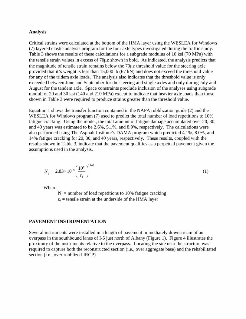
Analysis Critical strains were calculated at the bottom of the HMA layer using the WESLEA for Windows (7) layered elastic analysis program for the four axle types investigated during the traffic study. Table 3 shows the results of these calculations for a subgrade modulus of 10 ksi (70 MPa) with the tensile strain values in excess of 70με shown in bold. As indicated, the analysis predicts that the magnitude of tensile strain remains below the 70με threshold value for the steering axle provided that it’s weight is less than 15,000 lb (67 kN) and does not exceed the threshold value for any of the tridem axle loads. The analysis also indicates that the threshold value is only exceeded between June and September for the steering and single axles and only during July and August for the tandem axle. Space constraints preclude inclusion of the analyses using subgrade moduli of 20 and 30 ksi (140 and 210 MPa) except to indicate that heavier axle loads than those shown in Table 3 were required to produce strains greater than the threshold value. Equation 1 shows the transfer function contained in the NAPA rubblization guide (2) and the WESLEA for Windows program (7) used to predict the total number of load repetitions to 10% fatigue cracking. Using the model, the total amount of fatigue damage accumulated over 20, 30, and 40 years was estimated to be 2.6%, 5.1%, and 8.9%, respectively. The calculations were also performed using The Asphalt Institute’s DAMA program which predicted 4.1%, 8.0%, and 14% fatigue cracking for 20, 30, and 40 years, respectively. These results, coupled with the results shown in Table 3, indicate that the pavement qualifies as a perpetual pavement given the assumptions used in the analysis.
3.1486
6 102.83 10ft
Nε
− ⎛ ⎞= × ⎜ ⎟
⎝ ⎠ (1)
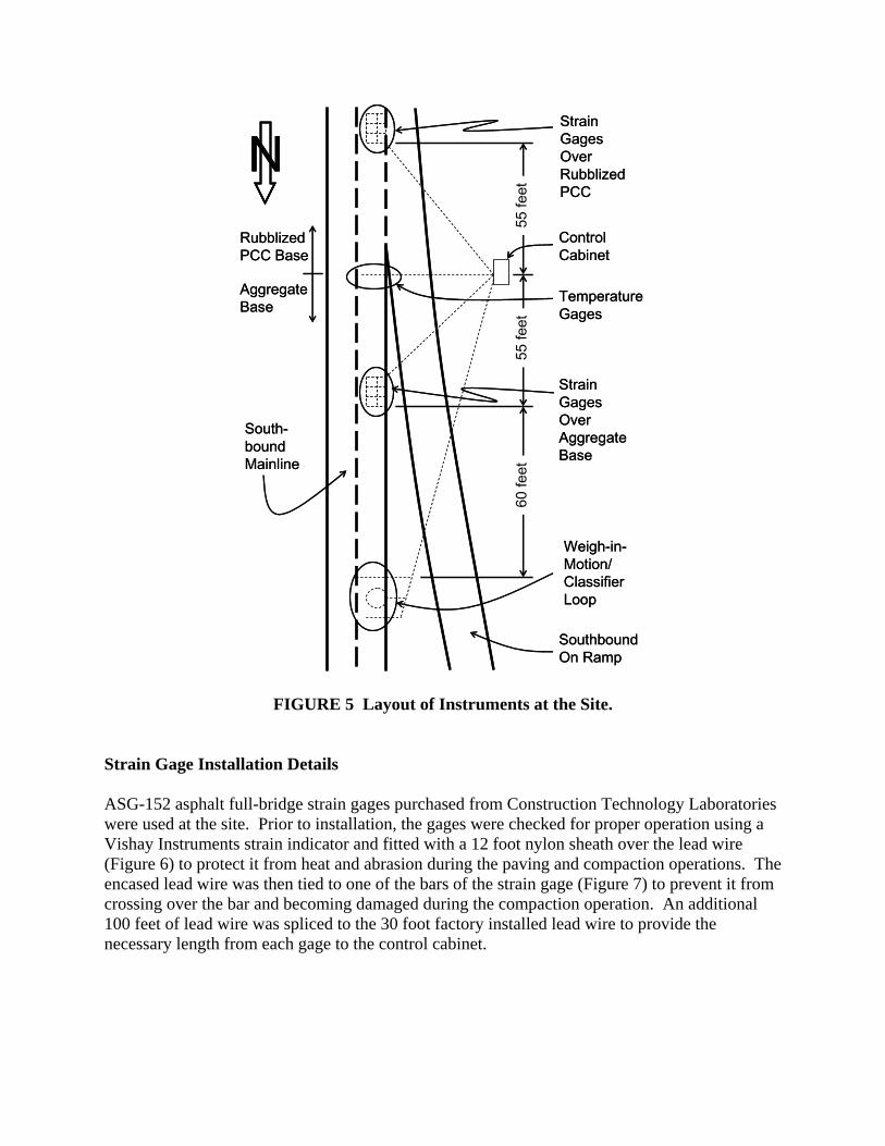
Where: Nf = number of load repetitions to 10% fatigue cracking εt = tensile strain at the underside of the HMA layer PAVEMENT INSTRUMENTATION Several instruments were installed in a length of pavement immediately downstream of an overpass in the southbound lanes of I-5 just north of Albany (Figure 1). Figure 4 illustrates the proximity of the instruments relative to the overpass. Locating the site near the structure was required to capture both the reconstructed section (i.e., over aggregate base) and the rehabilitated section (i.e., over rubblized JRCP).
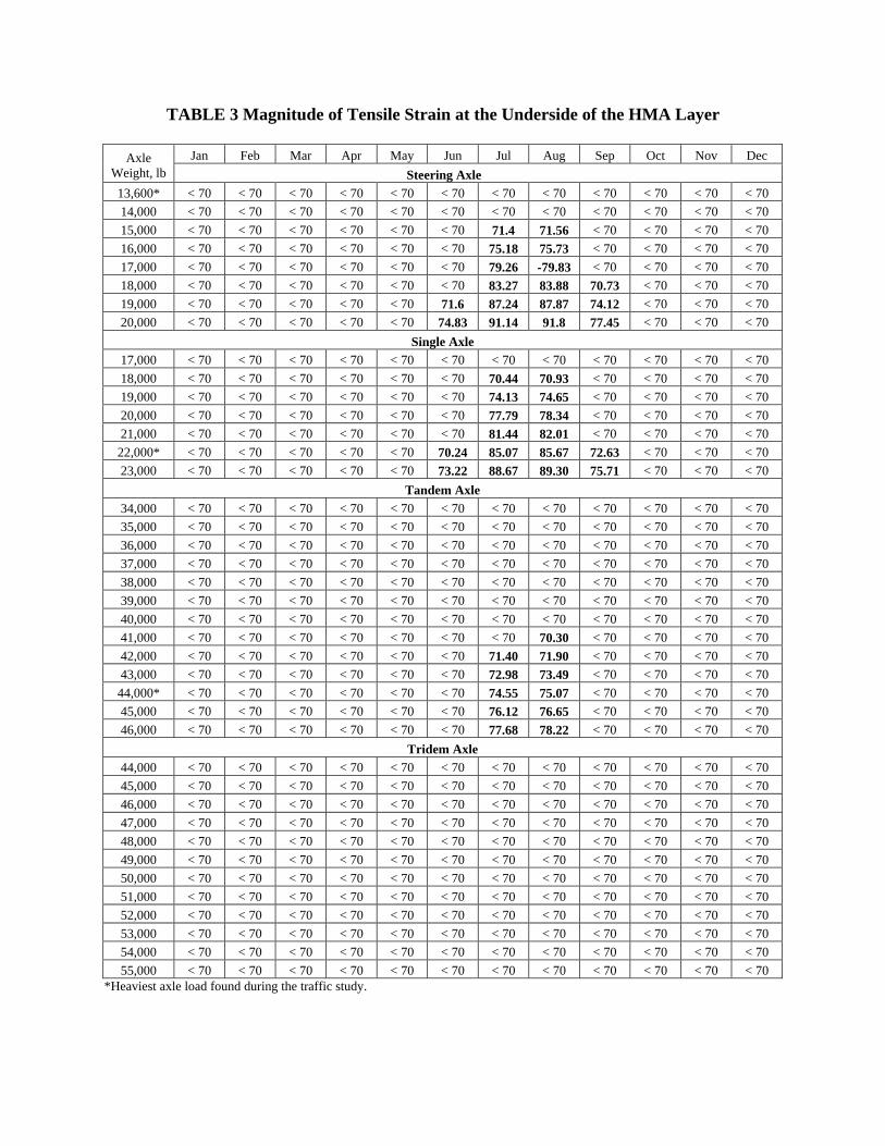
TABLE 3 Magnitude of Tensile Strain at the Underside of the HMA Layer
Jan Feb Mar Apr May Jun Jul Aug Sep Oct Nov Dec Axle Weight, lb Steering Axle 13,600* < 70 < 70 < 70 < 70 < 70 < 70 < 70 < 70 < 70 < 70 < 70 < 70 14,000 < 70 < 70 < 70 < 70 < 70 < 70 < 70 < 70 < 70 < 70 < 70 < 70 15,000 < 70 < 70 < 70 < 70 < 70 < 70 71.4 71.56 < 70 < 70 < 70 < 70 16,000 < 70 < 70 < 70 < 70 < 70 < 70 75.18 75.73 < 70 < 70 < 70 < 70 17,000 < 70 < 70 < 70 < 70 < 70 < 70 79.26 -79.83 < 70 < 70 < 70 < 70 18,000 < 70 < 70 < 70 < 70 < 70 < 70 83.27 83.88 70.73 < 70 < 70 < 70 19,000 < 70 < 70 < 70 < 70 < 70 71.6 87.24 87.87 74.12 < 70 < 70 < 70 20,000 < 70 < 70 < 70 < 70 < 70 74.83 91.14 91.8 77.45 < 70 < 70 < 70
Single Axle 17,000 < 70 < 70 < 70 < 70 < 70 < 70 < 70 < 70 < 70 < 70 < 70 < 70 18,000 < 70 < 70 < 70 < 70 < 70 < 70 70.44 70.93 < 70 < 70 < 70 < 70 19,000 < 70 < 70 < 70 < 70 < 70 < 70 74.13 74.65 < 70 < 70 < 70 < 70 20,000 < 70 < 70 < 70 < 70 < 70 < 70 77.79 78.34 < 70 < 70 < 70 < 70 21,000 < 70 < 70 < 70 < 70 < 70 < 70 81.44 82.01 < 70 < 70 < 70 < 70 22,000* < 70 < 70 < 70 < 70 < 70 70.24 85.07 85.67 72.63 < 70 < 70 < 70 23,000 < 70 < 70 < 70 < 70 < 70 73.22 88.67 89.30 75.71 < 70 < 70 < 70
Tandem Axle 34,000 < 70 < 70 < 70 < 70 < 70 < 70 < 70 < 70 < 70 < 70 < 70 < 70 35,000 < 70 < 70 < 70 < 70 < 70 < 70 < 70 < 70 < 70 < 70 < 70 < 70 36,000 < 70 < 70 < 70 < 70 < 70 < 70 < 70 < 70 < 70 < 70 < 70 < 70 37,000 < 70 < 70 < 70 < 70 < 70 < 70 < 70 < 70 < 70 < 70 < 70 < 70 38,000 < 70 < 70 < 70 < 70 < 70 < 70 < 70 < 70 < 70 < 70 < 70 < 70 39,000 < 70 < 70 < 70 < 70 < 70 < 70 < 70 < 70 < 70 < 70 < 70 < 70 40,000 < 70 < 70 < 70 < 70 < 70 < 70 < 70 < 70 < 70 < 70 < 70 < 70 41,000 < 70 < 70 < 70 < 70 < 70 < 70 < 70 70.30 < 70 < 70 < 70 < 70 42,000 < 70 < 70 < 70 < 70 < 70 < 70 71.40 71.90 < 70 < 70 < 70 < 70 43,000 < 70 < 70 < 70 < 70 < 70 < 70 72.98 73.49 < 70 < 70 < 70 < 70 44,000* < 70 < 70 < 70 < 70 < 70 < 70 74.55 75.07 < 70 < 70 < 70 < 70 45,000 < 70 < 70 < 70 < 70 < 70 < 70 76.12 76.65 < 70 < 70 < 70 < 70 46,000 < 70 < 70 < 70 < 70 < 70 < 70 77.68 78.22 < 70 < 70 < 70 < 70
Tridem Axle 44,000 < 70 < 70 < 70 < 70 < 70 < 70 < 70 < 70 < 70 < 70 < 70 < 70 45,000 < 70 < 70 < 70 < 70 < 70 < 70 < 70 < 70 < 70 < 70 < 70 < 70 46,000 < 70 < 70 < 70 < 70 < 70 < 70 < 70 < 70 < 70 < 70 < 70 < 70 47,000 < 70 < 70 < 70 < 70 < 70 < 70 < 70 < 70 < 70 < 70 < 70 < 70 48,000 < 70 < 70 < 70 < 70 < 70 < 70 < 70 < 70 < 70 < 70 < 70 < 70 49,000 < 70 < 70 < 70 < 70 < 70 < 70 < 70 < 70 < 70 < 70 < 70 < 70 50,000 < 70 < 70 < 70 < 70 < 70 < 70 < 70 < 70 < 70 < 70 < 70 < 70 51,000 < 70 < 70 < 70 < 70 < 70 < 70 < 70 < 70 < 70 < 70 < 70 < 70 52,000 < 70 < 70 < 70 < 70 < 70 < 70 < 70 < 70 < 70 < 70 < 70 < 70 53,000 < 70 < 70 < 70 < 70 < 70 < 70 < 70 < 70 < 70 < 70 < 70 < 70 54,000 < 70 < 70 < 70 < 70 < 70 < 70 < 70 < 70 < 70 < 70 < 70 < 70 55,000 < 70 < 70 < 70 < 70 < 70 < 70 < 70 < 70 < 70 < 70 < 70 < 70
*Heaviest axle load found during the traffic study.

N
Dever-Conner Rd. Overpass
≈25
0 ft
Instruments
ControlCabinet
Approximate limits of reconstructed section.
Rub
bliz
ed J
RC
P B
ase
Rub
bliz
ed J
RC
P B
ase
Aggr
egat
e Ba
se
NN
Dever-Conner Rd. Overpass
≈25
0 ft
Instruments
ControlCabinet
Approximate limits of reconstructed section.
Rub
bliz
ed J
RC
P B
ase
Rub
bliz
ed J
RC
P B
ase
Aggr
egat
e Ba
se
FIGURE 4 Location of Instruments Relative to the Overpass. Instrumentation Overview Using the procedures developed by the National Center for Asphalt Technology (NCAT) (8) as an installation guide, four temperature gages and 24 strain gages (12 over the aggregate base and 12 over the rubblized JRCP) were installed at the site as illustrated in Figure 5. In addition, a weigh-in-motion (WIM) device and classifier loops were installed upstream of the strain gages (Figure 5) so that the WIM device could trigger data collection.
RubblizedPCC Base
AggregateBase
Control Cabinet
55 fe
et55
feet
60 fe
et
Strain Gages Over Rubblized PCC
Strain Gages Over Aggregate Base
South-bound Mainline
Southbound On Ramp
N
Weigh-in-Motion/ Classifier Loop
Temperature Gages
RubblizedPCC Base
AggregateBase
Control Cabinet
55 fe
et55
feet
60 fe
et
Strain Gages Over Rubblized PCC
Strain Gages Over Aggregate Base
South-bound Mainline
Southbound On Ramp
NN
Weigh-in-Motion/ Classifier Loop
Temperature Gages
FIGURE 5 Layout of Instruments at the Site.
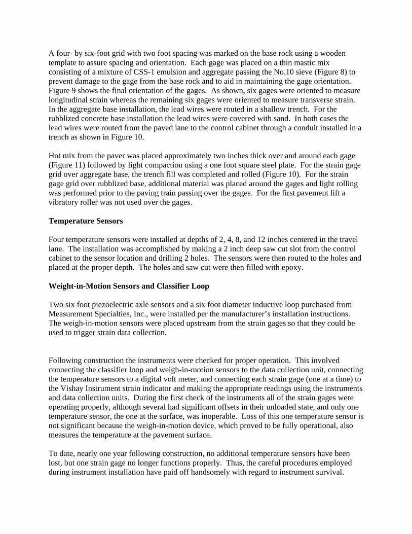
Strain Gage Installation Details ASG-152 asphalt full-bridge strain gages purchased from Construction Technology Laboratories were used at the site. Prior to installation, the gages were checked for proper operation using a Vishay Instruments strain indicator and fitted with a 12 foot nylon sheath over the lead wire (Figure 6) to protect it from heat and abrasion during the paving and compaction operations. The encased lead wire was then tied to one of the bars of the strain gage (Figure 7) to prevent it from crossing over the bar and becoming damaged during the compaction operation. An additional 100 feet of lead wire was spliced to the 30 foot factory installed lead wire to provide the necessary length from each gage to the control cabinet.
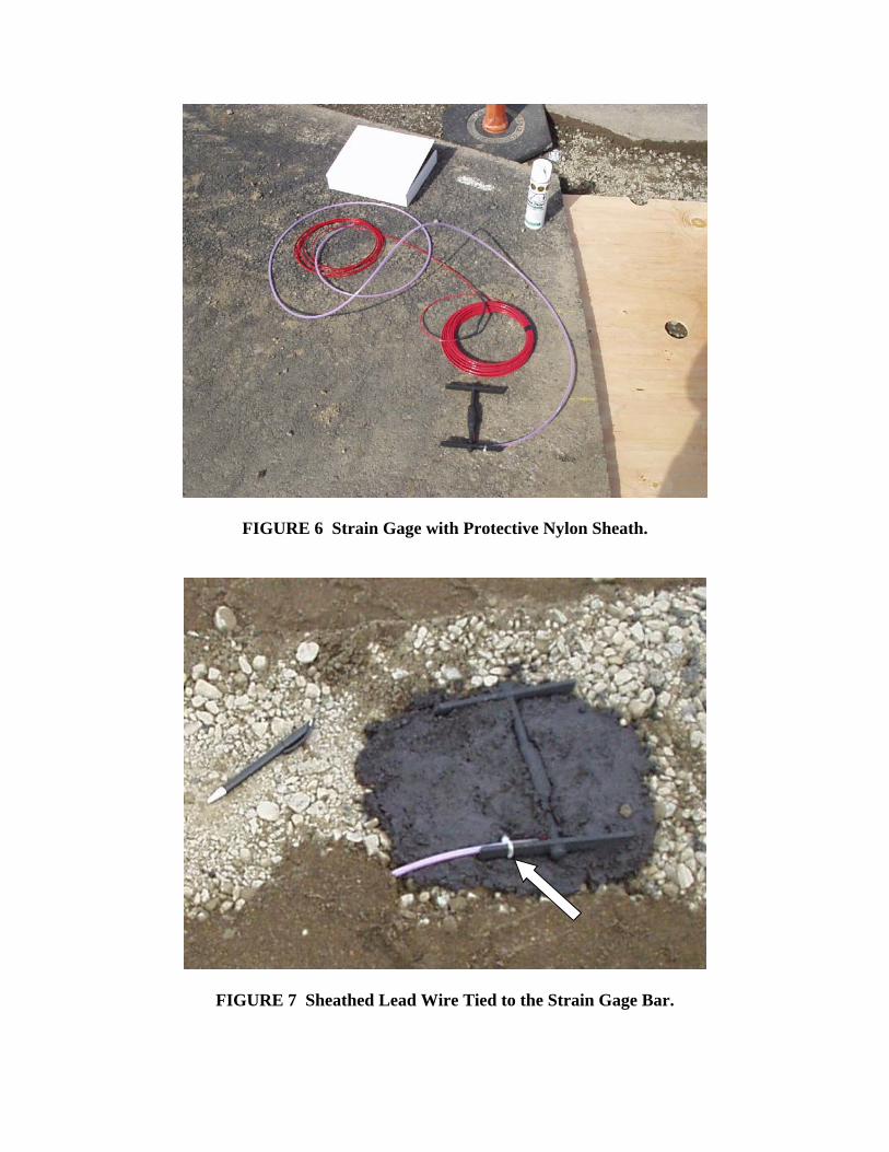
FIGURE 6 Strain Gage with Protective Nylon Sheath.
FIGURE 7 Sheathed Lead Wire Tied to the Strain Gage Bar.
A four- by six-foot grid with two foot spacing was marked on the base rock using a wooden template to assure spacing and orientation. Each gage was placed on a thin mastic mix consisting of a mixture of CSS-1 emulsion and aggregate passing the No.10 sieve (Figure 8) to prevent damage to the gage from the base rock and to aid in maintaining the gage orientation. Figure 9 shows the final orientation of the gages. As shown, six gages were oriented to measure longitudinal strain whereas the remaining six gages were oriented to measure transverse strain. In the aggregate base installation, the lead wires were routed in a shallow trench. For the rubblized concrete base installation the lead wires were covered with sand. In both cases the lead wires were routed from the paved lane to the control cabinet through a conduit installed in a trench as shown in Figure 10. Hot mix from the paver was placed approximately two inches thick over and around each gage (Figure 11) followed by light compaction using a one foot square steel plate. For the strain gage grid over aggregate base, the trench fill was completed and rolled (Figure 10). For the strain gage grid over rubblized base, additional material was placed around the gages and light rolling was performed prior to the paving train passing over the gages. For the first pavement lift a vibratory roller was not used over the gages. Temperature Sensors Four temperature sensors were installed at depths of 2, 4, 8, and 12 inches centered in the travel lane. The installation was accomplished by making a 2 inch deep saw cut slot from the control cabinet to the sensor location and drilling 2 holes. The sensors were then routed to the holes and placed at the proper depth. The holes and saw cut were then filled with epoxy. Weight-in-Motion Sensors and Classifier Loop Two six foot piezoelectric axle sensors and a six foot diameter inductive loop purchased from Measurement Specialties, Inc., were installed per the manufacturer’s installation instructions. The weigh-in-motion sensors were placed upstream from the strain gages so that they could be used to trigger strain data collection. Following construction the instruments were checked for proper operation. This involved connecting the classifier loop and weigh-in-motion sensors to the data collection unit, connecting the temperature sensors to a digital volt meter, and connecting each strain gage (one at a time) to the Vishay Instrument strain indicator and making the appropriate readings using the instruments and data collection units. During the first check of the instruments all of the strain gages were operating properly, although several had significant offsets in their unloaded state, and only one temperature sensor, the one at the surface, was inoperable. Loss of this one temperature sensor is not significant because the weigh-in-motion device, which proved to be fully operational, also measures the temperature at the pavement surface.
To date, nearly one year following construction, no additional temperature sensors have been lost, but one strain gage no longer functions properly. Thus, the careful procedures employed during instrument installation have paid off handsomely with regard to instrument survival.
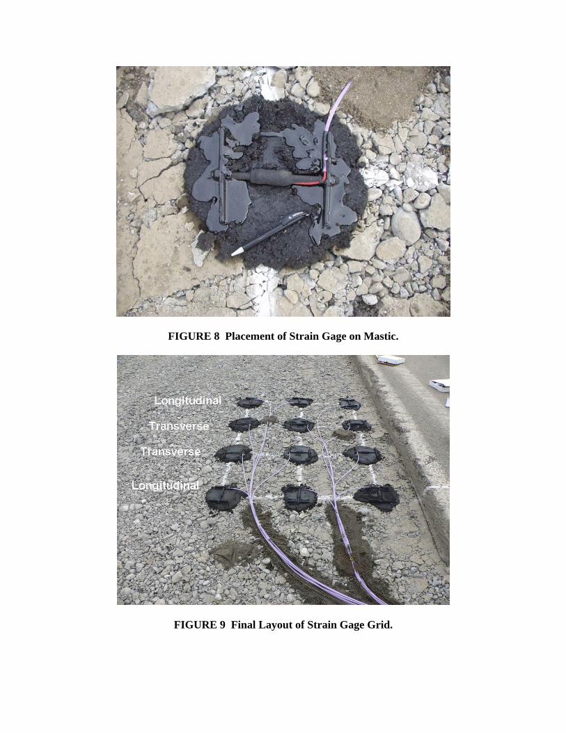
FIGURE 8 Placement of Strain Gage on Mastic.
FIGURE 9 Final Layout of Strain Gage Grid.
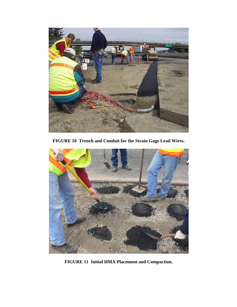
FIGURE 10 Trench and Conduit for the Strain Gage Lead Wires.
FIGURE 11 Initial HMA Placement and Compaction.

Strain Measurement Strain measurement is accomplished using a StrainBook (8 channels) and two WBK16 expansion modules (8 channels each) manufactured by IOtech, Inc. so that all 24 strain gages can be interrogated simultaneously. Setting up and configuring the data collection unit required several site visits owing to some unforeseen issues with the device. The most significant issue involved the offsets of the strain gages in that the offset essentially amounted to an unbalanced strain gage bridge. Although the StrainBook can electronically balance a strain gage bridge, it cannot balance a bridge that is significantly unbalanced. Because all of strain gages over the aggregate base and two of the gages over the rubblized JRCP were significantly unbalanced (some on the order of 15,000με), the incoming signals from these gages were simply outside the range that could be balanced by the StrainBook. Due to this, the signals could not be amplified sufficiently resulting in a very noisy signal. The solution to this problem was to balance the strain gage bridges using a shunt resistor across one leg of the strain gage bridge such that the output of the unloaded bridge was essentially zero volts. This was accomplished inside the StrainBook and WBK16 modules using resistance values scaled to the amount the bridges were unbalanced. PRELIMINARY DATA Although the weigh-in-motion device is operational and has been calibrated, it was not possible at the time of this writing to collect simultaneous weight and strain data. Thus, only strain data is presented herein. Nevertheless, several inferences are drawn from the data presented. Once the strain gages were properly balanced using the shunt resistors, all gages could be sufficiently amplified to obtain high quality data as evidenced in Figure 12 showing the response of the gages under loads applied by different types of vehicles. Several observations can be made from these data including:
• The axle loads in all cases are clearly discernable. For example, the passenger car and school bus were two-axle vehicles, whereas the loaded truck was a five-axle vehicle (standard 18-wheeler). With vehicle velocity information provided by the weigh-in-motion device, it will be possible to obtain highly accurate axle spacing information.
• The pavement experienced compression in the longitudinal direction several feet ahead of the wheel load applied by the steering axle before experiencing tension (characterized by the large, upward spikes in the data). This is also true between axle loads. This response is consistent with that found by the researchers at the NCAT Test Track (9). As will be shown later, the pavement does not necessarily experience compressive strain in the transverse direction.
• The maximum strain induced by the passenger vehicle (e.g., Pontiac Grand Prix) was only about a quarter of that induced by the loaded truck.
• The maximum tensile strain induced by the drive axle of the loaded school bus was actually higher (by about 30%) than that induced by the steering axle of the loaded truck.
• In all cases, the magnitude of longitudinal tensile strain was greater in the HMA over aggregate base relative to that in the HMA over the rubblized JRCP. This is not

surprising given that the section over the rubblized concrete is a thicker structural section (see Figure 2).
• Also evident from the data is that the strain energy quickly dissipated to a state consistent with that before loading, indicating the structure was behaving in an essentially elastic manner. It should be noted that the air temperature at the time this data was obtained was about 62°F (17°C), so it would be expected that the pavement temperature was somewhat higher.
FIGURE 12 Strain Measurement Obtained from Vehicles of Different Weights. Figure 13 shows a comparison between the longitudinal and transverse strain induced by a loaded, five-axle truck over both types of base course. The pavement experienced compressive strain ahead of the steering axle and between axles in the longitudinal direction, but in the transverse direction, the pavement only experienced tensile strain. It is also clear from the data that the strain energy dissipated more slowly in the transverse direction as compared with the longitudinal direction, particularly over the aggregate base, likely indicating a more viscous response in the transverse direction. Currently, the site does not have a means of electronically determining the transverse location of a wheel load passing over the strain gage grids such as that installed at the NCAT Test Track (9). However, it is hypothesized that the wheel location can be accurately determined from the relative strain magnitudes measured by a set of three strain gages in the same longitudinal position but spread out in the transverse direction (e.g., the first set of three gages a vehicle passes over).

FIGURE 13 Comparison of Longitudinal and Transverse Strain. Figure 14 shows the longitudinal strains as measured by the first set of three strain gages a vehicle encounters (i.e., the northernmost set of strain gages over aggregate base). The data indicate that the “inside gage” registered a tensile strain approximately three-quarters the magnitude of that registered by the “outside gage”. Given that the “outside gage” and “inside gage” are four feet (1.2 m) apart, it is hypothesized that the wheel load is offset from the “middle gage” and closer to the “outside gage” by 1 foot (0.3 m). Further research is planned to verify this hypothesis. CONCLUSIONS Based on the contents of the information presented in this paper, the following conclusions appear warranted:
1. Attention to care during instrument installation can result in a high survival rate of the instruments.
2. The thick HMA pavement layer over the rubblized jointed reinforced concrete pavement appears to meet the criteria of a perpetual pavement based on the mechanistic-empirical analysis presented herein.

FIGURE 14 Relative Longitudinal Strain Magnitude in the Transverse Direction.
3. Preliminary measurements of longitudinal and transverse strain to date indicate that the tensile strain at the underside of the HMA layer is less than the commonly accepted threshold value of 70με for initiation of fatigue cracking; hence, providing further evidence that the pavement sections are perpetual pavements.
4. The signals obtained from the strain gage grids can accurately discern differences amongst axle loads ranging from passenger cars to heavily loaded cargo trucks.
5. Measurements from the strain gage grids allow investigation of the relative importance of longitudinal versus transverse strain induced by axle loads of varying weight.
ACKNOWLEDGEMENTS The Authors acknowledge and appreciate the financial support for this project provided by the Oregon Department of Transportation and the Federal Highway Administration. Special appreciation is extended to Mr. Andrew Brickman for his contributions during the installation of the instruments as well as for his unending commitment to ensuring that the instruments and data collection units function properly.

REFERENCES
1. Guidelines for Use of HMA Overlays to Rehabilitate PCC Pavements, National Asphalt Pavement Association Information Series 117, Lanham, Maryland, 1994.
2. Rubblization, National Asphalt Pavement Association Information Series 132, Lanham, Maryland, 2006.
3. AASHTO Guide for Design of Pavement Structures, American Association of State Highway and Transportation Officials, Washington, D.C., 1993.
4. Samuel H. Carpenter, Khalid A. Ghuzlan, and Shihui Shen, “Fatigue Endurance Limit for Highway and Airport Pavements,” Journal of the Transportation Research Board, Transportation Research Record 1832, 2003, pp 131-138.
5. Hwang, D., and Witczak, M.W., Program DAMA (Chevron), User's Manual, Department of Civil Engineering, University of Maryland, 1979.
6. N. Sivaneswaran, Linda M. Pierce, and Joe P. Mahoney, Evercalc Pavement Backcalculation Program Version 5.20, Materials Laboratory, Washington State Department of Transportation, March 2001.
7. WESLEA, written by Fans Van Cauwelaert, Departement Des Constructions, Mons, Belgique, 1987, modified by Don R. Alexander, USAE Waterways Experiment Station, Vicksburg, MS, 1989. WESLEA for Windows Version 3.0, developed by Timm, D., Birgisson, B., and Newcomb, D., 1999.
8. Timm, D.H., Priest, A.L., and McEwen, T.V. Design and Instrumentation of the Pavement Structure Experiment at the NCAT Test Track. NCAT Report 04-01, National Center for Asphalt Technology, April 2004.
9. Priest, A.L. and Timm, D.H., “A Full-Scale Pavement Study for Mechanistic-Empirical Pavement Design,” Journal of the Association of Asphalt Paving Technologists, Volume 74, 2005, pp 519-556.