INSTITUTE OP THEORETICAL

AND EXPERIMENTAL PHYSICS

ITEP - 43

F,A«Berezin , M.S.Marinov

PARTICLE SPIN DYNAMICS AS THE GRASSMAN:;

VARIANT OF CLASSICAL MECHANICS

M O S C O W 1 9 7 6

INSTITUTE OF THECEEXICAL AHD EXPERIMEHTAL PHYSICS

ITEP - 43

F.A.Beresin -Department of Mathematics,Moscow State University

M.S.Jferinov -ITEP

PARTICLE SPIN DYNAMICS AS THE GHASSMANJT VAHIAHT

OF CLASSICAL MECHANICS

Moscow , 1976

621.3В4.6.Ш M-I6

A generalisation of the classical mechanics is presen-

ted. The dynamical variables fcf auctions-cm—«ге~р"йазе~враее^

are assumed to be elements of an algebra with anticommuting

generators (the Grassmann algebra). The action functional

and the Poisson brackets are defined. The equations of motion

are deduced from the variational principle. The dynamics is

described also by means of the Liouville equation for the

phase-space distribution. The canonical quantization leads

^to the Fermi (anticommutator) commutation relations. The

phaae-space path, integral approach to the quantum theory is

also formulated. The theory is applied to describe the par-

ticle spin^ln the nonrelativistic case, the elements of the

phase-space еле anticommtiag three-vectors £ , trsnsfor-

med to the Pauli. matrices after the quantization: ~€ ж

* ( it /2)Уг£[ «^Classical description of the spin preces-

sion and of the spin-orbital forces is given.-To introduce

the relativistic spin in an invariant шаппегхше needs a fi-

ve-dimensional phase space (a four-veottfr plus a scalar).

The bagrangian is singular and there is a constraint» resul-

ting from a "supersymmetry". The quantized phase-space ele-

ments are proportional to the Dirac matrices ifj^ aod У1 ,

while the constraint is transformed to the Dirac equation.

The phase-space distribution and the interaction with an ex-

ternal field are also considered.

© ИТЭФ. №76

C o n t e n t sPages

I. Introduction • 5

1.1. Physical Background ................ 5

1.2. Mathemanical Background g

1.3» Results and Discussion ............. g

II. Nonrelativistic Spin Dynamics

2.1. Classical Action Principle and 10Equations of Motion

2.2. The Phase-Space Distribution and т4

Observables *

2.J. The Canonical Quantisation

2.4. Path Integial for Green'sfunction 19

2.5» Motion in a Central Potentialwith Spin-Orbital Forces p

III. Relativistic Spin and the Dirac Equation

3.1. Classical Action and the 9

,Symmetries

3.2. Quantization and the DiracEquation 28

3.3. Particle in an External Field 32

Г7. Concluding Remarks 34

Appendices

A. Grassmann Algebra: Basic Definitions

and Results 36B. Operators ard their Symbols 39С Representation of Green's function

by Means of thu Phase-Space PathIntegral 44

i . птаовисмот

1.1* Ehysical Background

During the past few years a not so familiar concept has

emerged in high-energy physics, that of "anticommuting c-num-

oers". The formalism of the Grassmann. algebra is well known

to mathematicians and used for a long time. The analysis on

the Grassmann algebra was developped and exploited in a sys-

tematic way in applying the generating functional method to

the theory of second quantization [ij . This method was also

used for the theory of fermion fields in a textbook by Hse-

wuski [ 2J . Seemingly, the first physical work dealing with

~he anticommu'Cing numbers in connection with fei ions was

-hat by Matthews and Salam f ?J • The anticommuting c-numbers

and the "Lie algebra with anticommutators" (i.e. the Z2-gra-

ded Lie algebra) were the tools applied by Gervais and Saki-

ta [ 4j to the dual theory. These authors invented the two-di-

mentional field-theoretical approach to the fermionic dual

models (those proposed by Ramond and Nevett-Schwartz) and used

the symmetry under the transformation with anticommuting para-

meters ("supergauge" transformations) to prove the no-fhotft

theorem. Naturally, anticommuting classical fields are necessa-

-v to construct the string picture of the fermionic dual mo-

dels; a highly shillful approach to this problem is presented

by Iwasaki and EikfcawaГ 5 j • Interest to the concept in view

was greatly increased by exciting new results obtained in

1974, elaborating the four-dimensional supersymmetry, disco-

vered previously by Golf and and LichtmanfeJ , and the forma-

lism of superspace (see e.g. the review report by Zumino [?],

where references to basic works on the subject may be found).

We present here an application of the analysis on Grass-

mann algebra to such a respectable problem as the Hamilton

dynaoics of a classical spinning particle. Boch nonrelativis-

tic and relativistic situations are considered. The first at-

tempt to treat the classical elativistic top dates as early

as 1926 and is du to Frenkel [8,9j . A review of subsequent

work along this line is given by Barut [iOJ . However, the

problem seems to be far from its exhaustive solution in terms

of the conventional approach. An evidence to that is the pa-

per by Hanson and Regge [i1J , where one may find a number of

further references. Our approach is essentially different as

it uses tho Grassmann algebra to describe the spin degrees of

freedom. Apart from the concrete physical application to spin

dynamics the present theory may be of some interest as an exam-

ple of a generalized Hamilton dynamics with the appropriate

quantization scheme.

1.2. Mathematical Background

Го define the classical mechanics in an abstract way

one needs three basic objects. 1) A differentiable manyfold

M, called the phase space. Local coordinates X-. may be

introduced in the manyfold M. In principle, no global coordi-

nates may exist, and even theydo, there may be no reasonable

definition of the canonical coordinate-momentum pairs.

2) "Che algebra Qf(M) of complex-valued differentiable fun-

ctions on U defined in terms of the usual sum and product ope-

rations .

3) A Lie algebra of the Foisson brackets in-tt(U), gi-

ven by means of a skew-symmetric tensor field td-g, (x)

(sum over repeated indeces is implied)'

for any f(x) and A (x) belonging to«t(M). The field

satisfies the condition

which is equivalent to the Jacotd identity. Physical obser-

vable s are real elements of &(M). Dynamics is a ontinuous

one-parameter isomorphism group on41(11), determined by a Ha-

milton function H(x) by means of the equation

for any element f(x), where the "time" t is the parameter

of the group.

A way to generalize the concept of the classical mecha—

E~.cs is to abandon the manifold Ш, the "material basis" of

гме mechanics, retaining only the algebraic construction:

ring and Lie algebra. The Grазsmarm variant is a simple exam-

ple of such an "ideal mechanics", for which the multiplica-

tion in the algebra is not commutative. The generalization is

rather straight-forward, because though the elements of the

Grrassmann algebra are not just functions, there are for them

meaningful analogues of such concepts of the conventional ana-

lysis as the differentiation, the integration, and the Lie

groups, as introduced in the work £"i2j (see also the review

7

article [13J ).

To quantise an ideal mechanics is to construct an as-

sociative algebra of operators in the Hilbert space, rela-

ted to the classical algebra and having some general proper-

ties, discussed in paper [27J , which may be formulated in

a purely algebraic way independently on the existence of a

material phase spn.ce. One may see that in the Grassmann ca-

se with the "flat" Poisson brackets ( ^ ^ is a constant

matrix) the operator algebra has a finite-dimensional repre-

sentation.

1.3» Results and Discussion

The basic idea of the present approach is to consider

eieaencs of a Grassmann algebra as classical dynamical varia-

bles, i.e. functions of the phase space. The action functio-

nal, the Hamiltoniaa and the Poisson brackets, as well as so-

me other concepts of the classical mechanics, are defined.

The receipt of quantization is to substitute the Foisson

bracket for the canonical variables by the anticommutator of

the corresponding operators (as usual, devided by -ill).So

af-оег the quantization the Grassmann algebra generates the

Clifford algebra.

The Grassmann algebra with three generators, transfor-

med as components of a three-vector under space rotations,

gives rise to the nonrelativistic spin dynamics. Quantized

canonical variables are represented by the Pauli matrices.

The Grassmann algebra with five generators, an axial vector

and a pseudoscalar, is necessary for description of the re-

lativistic spin. Quantized variables are expressed in terms

of che Dirac matrices. In the relativistic case the system,

describing a particle, is constrained in the spin phase spa-

ce, as well as in the orbital phase space. The spin const-

raint is just the Dirac equation. Thus after quantization

the present scheme reproduces the well known Pauli-Dirac

cheory of the spinning electron. A brief account of our re-

sults was published previously [i4-j •

The quanta! action for anticommuting canonical variab-

les was written first by Schwinger [ 15J , who named them va-

riables of the second kind. However, the classical —nliinii •

and the theory of a relativistic spinning particle was not

considered by Schwiager; this author had in mind the quanti-

zed electron fields necessary for his formulation of the r

quantum electrodynamics. No clear statement that She classi-

cal variables not only anticommute, but have also zero squ-

are , may be found in the work by Schwinger. He also argued

that the number of the second-kind variables must be even

(note, that in our construction the phase space is odd-dimen-

sional), so that complex-conjugated coordinate-momentum pairs

may be defined. No particular mechanical system was discussed

by Schwinger. Perhaps our theory is useful as a simple exam-

ple to Schwinger's variations! formulation of the quantum

f.eia theory "' • The idea to consider the generalisation of

.e classical mechanics on a ring with arbitrary generators

was suggested by Martin [1б1 , who also presented a nonrela-

tivistic top as example of mechanics on a ring with anticom-

muting generators. Unfortunately, we were not aware of this

interesting work in time of our first publication £14] and

did not mentioned it. The progress of the theory of supersym-

metry provoked an interest to the classical mechanics in the

*' A Lagrangian formalism for spin variables, extendingSchwinger*s variational principle, was constructed ЪуVolkov and Peletminsky [52J .

superspace, in other words, to the theory of diffeomorphism

groups on the Grassmann algebras; an evidence to that is a

note by DeWitt [ 17J .

In Section II, the nonrelativistic spinning particle is

considered. The classical action princip'e is formulated.

The phase-space dynamics based on the Liouville equation is

developed. The canonical quantization is discussed in general

and reconstruction of the conventional formalism is shown.

The раЛintegral in the Grassmann phase space is defined;

the quanta! Green's function for precession of spin in a

constant field is calculated by this method. The theory of

a relativistic spinning particle is presented in Section III.

It is snown that in the invariant description of a free par-

ticle there are two symmetries, "gauge" and "supergauge". The

quantization is done and the Dirac equation is deduced. The

case of external field is also considered and the B*rgmann-

-ulichel-Telegdi equation is obtained in the classical mecha-

nics. Some necessary results, published previously, are pre-

sented in the iLost appropriate form in Appendices. Results

on the Grassmann algebra are compiled in Appendix A. Phase-

space representation of quantal operators and the phase-spa-

ce path integral for Green's function in case of the conven-

tional cheory are considered in Appendices В and С

II. KOKRELATIVI3TIC SPIN DYNAMICS

2.1. Classical Action Principle and aquations of

Motion

Suppose that the dynamical variables, describing the

nonrelativistic spin dynamics, зге elements of the Grassmann

algebra & , with three real generators £ , i = 1,2,3

10

(for definitions see Appendix A.). Define the phase-apace

trajectory Дг (t) as an odd element of Q. , depending

on a time parameter t . Introduce the classical action as

a functional of /*(t) and suppose it is an even real ele-

ment of # , . Write it in a form analoguous to the Hamilto-

nian action ( cf. Bq. (СИ)):

where H( С ) is an even real function of A , the Hamilto-

nian, i = d fi /dt;, and U) is a symmetric imaginary mat-

rix ( Ы is anti-Hermitian, as in the conventional mechanics).

By means of a linear transformation b) may be .educed to

the simplest form

(2.2)

Note that the first term in £q. (2.1) is not a complete deri-

vative, because A and £ anticommute. As any element of

, H( P ) is a polynomial of a degree, no more than 5.

Only even terms may be present; so, omitting an inessential

constant, the most general form of the Hamiltonian is

& f M. > (2.5)= "

where b^ are r e ai numberA

The equations of motion are obtained under the conditi-

on that the variation of «A be zero:

~ ̂ Ли, 4 f

where *K S Э /*ff, •

i a t n e right derivative. The eo-

lation of this equation is evident

l 2.

5 )

where R is an orthogonal matrix describing the rotation

with the angular velocity b • This solution may be inter-

preted as the spii. precession in an external ir^gnetic field

В , where b = ЭС В and at is the magnetic moment. An ex-

plicit cime dependence of b is also possible. The Eamilto-

nian (2.5)i a bilinear function on the phase space, is an

analogue of еде oscillator. A formal equivalence between the

spin precession and the Permi oscillator was also noted in

another context [18J .

In accordance with £q. (2.4) define the Poisson brackets

for any pair of dynamical variables

f ={И,{}рв (2.7)

Evidently, the Poisson brackets are antisymmetric if f and

£ are even elements of vhe Grassmann algebra and if f is

an even element while £ is an. odd element. In case f and

£ are odd elements the Poisson brackets are symmetric* The

graded version of Jacobi's identity is also valid. So the al-

gebra defined by 3q. (2.6) is a Z 2 -graded Lie algebra (see

e.g. the definition in Г12] or M5J ). Рог the canonical va-

riables the Poisson brackets are

P.8. *' (2

'8)

12

The rotation group in the Graaamann phase space is genera-

ted by the spin angular momentum

( г и о )

The classical mechanics of a nonrelativistic particle

with spin is constructed in the phase "superspace" consisting

of the six-dimensional obrital subspace (a^, р̂ .) and the

three-dimensional spin Grassmann subspace. The most general

action describing a particle in a local external field is

where 1^ = £ . %sP*i ^"(^^B^k iS th& orbital anSu~lar momentum ,VQ(q) and V̂ .(q) are potential functions у B(q)

is a vector field. The term with 7^ in Eq. (2.11) is the spin-

orbital interaction. The equation of motion derived from the

variational principle are

(2.12)

It is remarkable that in.presence of the spin—orbital inte-

raction the orbital subspace is not invariant, so q and

p are not just real numbers. The dynamics algebra is a

ring with 6 commuting and 3 anticommuting generators. The

equations are simplified in the case of sp-erical symmetry}

it is considered in some detail in Section 2.5.

2.2» The Phase-Space Distribution and Observables

Relation between an abstract mechanics and observable

quantities is established by means of a distribution func-

tion in the phase space. As in the conventional mechanics,

the dynamical principle for the Grassmann variant may be

formulated as a Cauchy problem for the distribution

t). The Loiuville equation is

the equations of mocion (2.4) are just its characteristics

equations. For any dynamical variable f ( P ) , its averaged

value is observed, which is a number

The integral is defined in Appendix A. It is appropriate to

assume that tiie distribution is an odd real element of Of:

> (2.15)

ПХ.

The distribution is normalised and д is the average spin

momentum

</>-/, <&>'£. »(2.16)

In case of motion (2.5) the vector о depends on the time

t , and the dependence is given by the same rotation matrix

R . So the average spin vector is subject to the precession.

To be an honest distribution the function P ( ? ) must

be non-negative in some sense. The usual way to generalize

the concept of positivity is to demand that the integral of

0 ff be non-negative for any function f. One may see that

this is true only in the -trivial сазе ^ = 0. Tnis is the re-

ason, why the Grassmann variant of the classical mechanics

can not be applied to the real world. It acquires a physical

meaning only after the quantization.

2.3. The Canonical Quantization

In accordance with the general rule of quantization (/I9J,

we replace the Poisson brackets for the canonical variables

in the Grassmann case by the anticommutator of the correspon-

ding operators, divided Ьу-гЛ:

(2.17)

Renormalizing the operators suitably, we get the Clifford al-

gebra with 3 generators:

"" 2.18)

The only irreducible representation of this algebra is two-di-

15

oensioaeut it is equivalent to that realized by the Pauli

matrices. Consequently,

4 ~ & * H i ь -t* К. [L & (2.19)

Note, that in the conventions! theory of the angular momentum

the starting poicT is the commutator, while the simple form

of the anticoamutator arises only in the spinor representa-

tion describing the spin 1/2. The present approach is inver-

se: the anticommutaoor (2.17) is postulated and therefore on-

ly the spinor representation is produced.

The operator corresponding to the phase-space distribu-

tion (2П5) is proportional to the usual density matrix

.3/tj> = г (*/t) (± t cv/%),

(2.20)

while the integral over the phase space is replaced by tra-

cing of Che representing matrix. Kote chat the matrix P is.

positive eemidefinite if 1 ^ 1 ^ 7fc/2. So, the purely quan-

tal nature of the spin manifests itself once more.

Tae Heisenberg equations of motion are obtained from

-iqs. (2.4) by means of the direct substitution» To get the

Sciiroedinger picture one has со introduce the spinor tp func-

tion, "factorizing" the density matrix О(~к)~ 4>(t) Xy O-A

Its time evolution is mastered by the Pauli equation. So the

usual taeory of the nonrelativistic spin 1/2 is reconstructed.

Now, it is appropriate to consider the case of the Grass-

aann algebra with any number of generators, (ftf . Evidently,

the construction of the classical mechanics, described for

Cn, , may be directly expanded to СЛ . The quantization

is defined by Bq. (2.17), and > ~ (~К/£) °]. ' - =

16

a 1, ..., n, where 6*fc are generators of the Clifford

algebra С . It is known that r

д has only one irreducible

Hermitian matrix representation. Its dimensionality is d =

г 2B for n i 2a or n = 2ш t 1, mis integer. (Note that the

matrix representation of Ot is 2? - dimensional). She

case of an even n is in closer analogy with the conventio-

nal theory, as one may introduce pairs of conjugated cano-

nical (complex) variables (q , pr ), г = 1,...,m, defining

^ » С f,+ t {^ ) / *"& . P1 = ( С f

1 f f

K )/VX = iqj" ,

q2 = ( t + i £ )/ fx, » etc. -he anticommutators are

Jusc this case was considered by Schwinger M5J • It is the

case of an odd n that is of interest for our purpose. A.

remarkable feature of Сд for odd n is that in the mat-

rix representation the generators are not independent,

^1 ̂ X • • • ̂ v = -^ ̂ *

I n < i e e d» *^

е Product: commutes with

any (J- and its square is -1, while its sign is reffered

к

to the choice between two classes of equivalent representati-

ons (right or left coordinate frames). Therefore, to make un-

яibiguous the classical counterpart of a quantal operator,

-.e has to declare whether it is an even element, or an odd

element of

Represent the quantal operators by their symbols, in

analogy with the usual quantum mechanics (see Appendix B).

For any operator g a polynomial representation may be

written

*<*... к? л А>. з С

2*

2 2)

t1 " cky

17

ik)where (2y are "c-mmber" totally antisymmetric tensors.

odd n, this fora is unique if only terms of a fixed pa-

rity are present. Thua any £ пае two equivalent decomposi-

tions, even and odd. Define an analogue of the Weyl symbol

for the operator

Sach operator has two symbols, even and odd. It may.be seen

that they are interrelated by a Fourier transformation. As

in the conventional theory, the Fourier transformation may

be used also to formulate the Weyl quantization. Relation

between an operator and its symbol is given by the integral

form

(2.24)

.25)

Неге й = ( О* .. .j PfA are generators of the Grassmann

algebra Oi , anticommuting with £ and С . Pro-

perties of the operator JL«. (P/ are similar to those of

the operator -Qft) , considered in Appendix B:

(We discuss now the case of an odd n, d » 2^n " is the

dimensionality). Using these formulae, one easily gets

(2.28)

This result enables one to find the symbol of the operator

g , if its parity is chosen (note, that £( У ) and g( J3 )

have opposite parities). The multiplication law for the sym-

bols is obtainable from 3q. (2.26)

Неге А ? « ? are regarded as three independent sets

of generators of the Grassmarm algebra UL .

We conclude this Section with she following resume. In

che Grassmann mechanics the quantal operators nave two rep-

resentations: by finite dimensional matrices and by elements

of ^he Grassmann algebra. This is quite similar to che usual

quancum mechanics, where the operators may be represented

either by functional kernels (say, in the coordinate space)

or :y their symbols, i.e. functions on the phase space.

2.4. Path Integral for Green's Function

The subject of this Section is to obtain an expression

for che operator

(t) ( i t H j (2.30)

In the Grassmann. case, The method is to calculate its symbol

C^ £ E ) in form of the phase-space path integral. This is

a direct generalization of the approach applied to the quan-

tum mechanics in a work by one of the authors f20J (see also

the Appendix C). It is quite natural to us^ this approach,

because in the Grassmann phase space one can not use the co-

ordinate - momentum language, and it is impossible to defi-

ne an analogue the Feynman path inuergal in the coordinate

(or momentum) space.

Represent che operator £^, t "W as an infinite pro-

duct of infinitesimal tine translations

Rewriting ;.iia form in terms of symbols and using the multi-

plication law (2.29) one gets Q /c -{- \ — 4x*** G\_

(2.52)

with che boundary condition 5 s 5 . Note that one

should regard X t Г ц и , as indeDen-

dent sets of (anticommuting) generators of the Grassmann al-

gebra. This formula is to be compared with Eq0 (C.4)<> One

may integrate over t . ,, f , get an analogue of

£q. (G.8) and write the formal expression

(2.33)

20

*here

However, only Eq. (2.J2) reveals the true meaning of the

functional integral, and it is useful for further analysis.

Apply the path integral approach to a simple example:

the spin precession in a constant magnetic field. The Hamil-

tonian is given Ъу Sq. (2.3) and may be rewritten also as

H( E ) = bS, where S is the kpin momentum (2.9). Using the

resemblance to the harmonic Jscilla*"9r we procee along the

same lines as in obtaining Sq. (C.16). In the present case

where Ъ = j Ъ J , n = b/b; we have used the fact that

(Sn) = 0. To get this result, we calculated the Gaussian

integrals over the Grassmann phase space by means of £q.(A.

I-. Jte that the cosine is now in the nominator, contrary to

Jq.(C,16). Using the symbol and Sq. (2.19) it is quite easy

to write the operator

and to reproduce the result that one obtains calculating

21

i J +eip(—i. v&L ) in a usual manner.

* — —

A number of authors used the concept of the path integ-

ral in space of anticommuting functions: Khalatnikov [21J ,

Matthews and Salam [3] , Candlin [22 J , Martin ̂ 23J and

others* A consisted mathematical formulation and the defini-

tion of the integral on the L^assmann algebra were given in.

paper [24j . On t..e other hand, some authors described the

spin dynamics by means of phase spaces with commuting ele-

ments : Schulman Г 25j , Bezak [26J (both considered the path

integrals), Berezin [ 27] , Tarsfci [28] , Hanson and Regge

[_11 J . The present approach seems to be the most adequate,

and spin of -he electron finds "a simple and ready represen-

tation" in -he method of path integrals, absent before, as

was stated in the booi by Feynman and Hibbs [29 / (p.355).

2.5. Motion in a central potential with Spin-Orbital

Forces

For a simple example, consider the motion of a spinning

particle influenced by forces presented by the Hamiltonian

(2.11), assuming that Ъ^ в 0 and that the potential functions

depend on R = j q / only. The intergals of motion are the to-

tal angular momentum /J = L + S, L and Л = IS (note

that S25 0 and Л = 0). From the equations (2.12) we get

for the radial motion'.

(2.38)

The problem is now reduced to that of motion with the effec-

tive potential TJ(&/— 1^ + ̂ /2*»^^I^containing a

nilpotent perturbation in the last term. Evidently, the so-

lution is to be represented in form

22

where f , £, a, pnd b are number functions. Substituting

into (2.38) one can see that r(t) and.p(t) are just the so-

lution of the problem with no account of the spin-orbital

potential, while a and b satisfy the linear equations

a. = b/m, b = -s(t)a - f (t) (2.40)

where

S(t) = V (r) + 5L2/mr4, f (t) = VJ( (r)

If the orbit is stable against small perturbation in the

classical sense, g(t) > 0 and (2.40) is the equation for an

oscillator with the frequency Гg(t)J ' and the driving

force f(t), which are constants in- case of a circular orbit.

Thus the solution is identical to the usual perturbation

theory in /\ , however it is exact, because higher powers

of^anish identically. To get the "observable" trajectory

one has to average over the spin variables, i.e. to integra-

te R(t) with the distribution (2.15). The result is that in

the final expression one should dubstitute Д by a cons-

tant < Л > s (cL), determined by the initial conditions.

As for the angular coordinate and spin, their motion

is mastered by the equations

S a 7̂ ,(1, X S ) *

£•• ^(SXDS ^ ( ^ X L)

where V. а 7д Г r(t)7 is a function of t . It is possib-

le to substitute R by r in the argument of ?1 in Eq.(2.M),

because Л S = 0, ( S X f ).=" О, and /\ (L XF )= 0. The

vectors £ , S, and L precess around the same fixed axis

Ч with the same anrular velocity, which is constant in ca-

se of a circular orbit.

III. RSLATIVISTIG SPIIT AND ТЕЗ DIRAC STATION

3.1. Classical Action and the Syagetrics

Construct the action for a relativistic spinning pirtic-

le, invariant under the full Poincare group and having1 the

nonrelativistic liniic, considered in Section 2.1. Assume

that ths spin variables are components of a four-vector £ .

However, an introduction of a new phase-space coordinate F

is not so inoffensive in view of two reasons. First, in the

nonrelativistic ii^ic a "second spin" ?, f would arize

and the representation of she rotation group would be redu-

cible. Seccnd, and more serious, is that one is not able to

quantize such a systen because of the Minkowski indefinite

metrics. Го get a consistent scheme (and to reconstruct the

Dirac theory) we assume that the action has an additional

syaaetry, so that f be in fact excluded froa the eaua-

uions of motion, even though, the equations are Lorentz-inva-

riant.

Start from the action

Неге Г is a mono tonic parameter labelling the points on the

particle world line, q. ( С ) are coordinates of the point,

q = dq^ / d T , ^ = d r /d T , the light velocity с я

= 1. Note that f are the phase-space elements, and (3*1)

may be considered as Routh's form of the action. Our metric

convention is (-, +, +, +), so *t = -1. The action is in-

variant under che reparanetrization of the trajectory $ C - *

T — ФСС) , where f(TJ is a monotonous

function. !he fundamental bilinear form for the £ variab-

les is degenerate , and there is no equation of motion for

che longitudinal component of the vector £ . To formula-

ce the dynamics, an additional constraint is necessary, and

to cake this constraint explicitly invariant int oduce a new

Grassmann variable fg . The constraint is

s0- С3.2)

To get a manifestly covariant canonical formalism for the

system having a singular Lagrangian one may apply Dirac's

method (the general approach is given in a boot by Dirac [30],

modern applications to the relativistic particle dynamics may

be found in papers by Hanson and Regge [11J and by Gasalbuo-

ni at, al. Г517 ). Add the constraint (5.2) with the Lagran-

ge multiplier A (anticommuting) to the original Lagrangi-

7;

The canonical momentum is

25

and the phase-space constraints are

p2 + m2 = 0, (p * ) + m P = 0 . (3.5)

With account of the constraints the Hamilton action is

(5.6)

where 1 is another Lagrange multiplier (commuting)-. The

equations of motion derived from the action principle are

. и =х/г- (3"7)

The first equation is consistent with (3.4) if

-€= (z-± fs */**)/* **,

ала the equation takes another form

An appearance of the second term in Eq. (3*9) might be anti-

cipated; it is the classical analogue of Sehroedinger*s Zit-

terbewegung (a discussion of this concept was presented by

Dirac fi9j t & 69, the algebraic aspects are considered by

Jordan and Mukunda [52] ). Note that the time evolution mi-

xes coordinate and spin degrees of freedom, just as in the

nonrelacivistic case with a spin-orbital potential (Cf. Bqs.

(2.12) )i the whole phase space of the relativistic spinning

particle is a "superspace".

The constraints (J.5)result from the invariance of the

action under two kinds of transformations* The first one

was mentioned; it is the "gauge" group, V-+T =s Ф(Т).

Дп infinitesоmal transformation of the second kind is

(3.10)

where h (_X) is an anticommuting "parameter" depending

on T* ambiguously. In analogy with the transformations in-

troduced in a dual model by Gervais and Sakita [41 we call

(3.10) the "supergauge" group. The variation of the action

(3.3), induced by (3.10) is

* « •

cC (fr

it vanishes if Ч (ТА — 1(^f)1!=^ • I*

i s rematkable

that both transformations, gauge and supergauge, change the

scale factor z , contrary to the Poincare group.

To fix a solution of the equations of motion (3.7),

(3.9) one has to choose the indefinite factors И and z

(or 1) in some way, i.e. to fix the supergauge and the gau-

рэ. As for z, two variants are used in case of no spin:

J.) ъ = 1, С is the self-time, and ii) z = WPO > T - q

Q

is the "laboratory" time. An appropriate choice of <Д is

not so evident. There are only 2 Poincare-invariant anticom-

muting elements in the phase space: f and ( P fffi ) S

5 £.*& fa ̂ $fff • I* one takes A «» fF , theequations of motion have no apparent T invariance. More app-

ropriate is the choice

27

(3.12)

where к is a real constant of dimension (action) . Kote

that if z = const, Я is also conserved. This choice is

rather convenient, because the second term in (3.9) vani-

shes identically and the notion of a free particle is quite

simple:

ОИЗ)

A defect of the ciaoice (3.12) is that it breaks the symmet-

ry under sotice reflections. Just as in the nonrelativistic

case, before the quantization one cannot decide whether f

is an axial vector (and ?_ is a pseudoscalar), or a vec-

tor (and ?_ is a scalar). However, parity of л given

cy (3.12) is opposite to the parity of f- in both the va-

riants. Го identify T wich the laboratory time q^ one may

put

1 = (2р0Г

1 , Л = fm^

o (5.1*)

where f is a scalar function of dimension (action) .

3.2. Quantization and the Dxrac Equation

The action (3.6) results in the canonical Poisson brac-

kets

J

(3.15)

where fly = diag(-1, +1, +1, +1), other brackets vanish.

Xhe commutation relations for the quanta! operators are

while the constraints (3«5) are converted into conditions

on the physical states

(J2 + »

2) + - 0 , (3.17a)

0 1 (3.17b)

The operators Л , с_ are generators of the Clifford

algebra C,-, its representation is four-dimensional and is

given by the Dirae-Pauli matrices:

(3.18)

where, as usual,

V" — ! #• V" У V + J

' V* J

(3.19)

jf0 and Jg are Hermitean, 01,1,} are antl-Heraitean.

Multiplying (3.17b) by ( t / 2 ) ~1 / 2 JT

S we get the Dirac

equation (р7Г+\г<\.) ]> = 0 . Conditions (3.17a) and

(3 17b) are consistent, as may be (and should be) checked

G ..-ectly. Uote that without the condition (3.17b) the quan-

tization would be inconsistent, because in view of (3*16)

— — К and anxadefinite metrics arises.

Generators of the Lorents group 7 are construe-

ted along the conventional linee

29

In the classical theory

(3.21)

R*- (3.22)

To get the quantal operators ait (anti) symmetrisation

is necessary

.23)

To construct a i-elatiTietic phase-space distribution,

like (2.1$), note tbat the components ( pf ) and P are

not observable and were introduced in order to sake the for-

Dalien invariant. So ve assume that P ^ f } = ^[(P$)/

$/? j О (? ) , «here S* depends on the transversal

components of ? only and is an odd element. Is it is

evident from definition of the integral on the Grassmaon al-

gebra (S9..U.6)), S ( ^kJ = ? . With all this in view,

«rite the phase-space distribution in a fora ready for the

quantisation

(3.25)

оГ is a real four-vector, ( V Л ) • 0, and

Ъ • 1/6a» as given by the nornaXisation

The function P C v ** "r***911 ***

a foril invariant under

tne supergauge transformations (3.10). The vector Vl la

a classical analogue of the Pauli-LubanafcL vector; it d«-

temines the averaged value of the spin aonentum, defined

by (3.21)

Рог a free particle -0^ is constant, as follows from the

Liouville equation for J*C$) •

To get the quanta! density matrix,substitute the ope-

rators (3*18) into (3.25)

>.28)

«here CL. = X^./% . This is just the fore introdu-

ced by Michel and lighten/"33? .

3.3» Particle In an External Field

To describe the interaction of a charged particle withни

an electromagnetic field A. (q) write the action as a sum

A = ^гее

+ ^ t »

w n e r e Afree

i s Siven by ^q. (3.1), and

0.29)

Here e_ is the charge, JC is che (total) magnetic moment

s 9/4 /Эф^ — 'ЪА'4'/ 2?У . The interaction of

spin with Che field was written as ( F S^jj ) by Eren-

kelГ s] • -his form was also analysed by Barut fiOJ and Han-

son and Regge j~111 . (Among many other papers on motion of

spin in a field mention the works by Suttorp and de Groot

(УН and Sllis Г35 J )» Dealing with the Grassmann variab-

les, one escapes some difficulties present in the previous

approaches.

The canonical momentum is

(3.30)

and the equations of mocion are

Besides the Zicterbewegung , present also in case of no

field, chere are two effects on the space-tine trajectory

due to the spin variables: a renormalization of the mass

32

and forces proportional to the derivatives of the field*

To obtain the Bargmann-Michel-Telegdi equation Гзб] t

describing the spin precession in a homogeneous field, «ri-

te the phase-space distribution (5.25) as follows

(3.32)

where /

W-|A.

i s a solution of the equation

and apply to it the Liouville equation in

(3.33)

Under the condition (b~£) + £ « 0,this equation is

equivalent to the following one

and we get the familiar result Г?б1 .

The interaction Lagrangian (3.29) is Lorentz-invariant

and gauge-invariant, but it breaks the supergauge symmetry.

The variation of the first term under (3.10) is

X -

Kote that the breaking is in a sense "minimal", i.e. propor-

tional to higher powers of ? , if there is no anomalous

magnetic moment and £ • e/2a. It is possible also to re-

duce the supergauge breaking, writing the first term in

(3*29) in a "superspace" fora: eA (Q)q , where Q ж

33

the reflation (3.35) vanish**.

i r . сонсыгагаа REMARKS

We have presented the Grasemann variant of the Hamil-

ton mechanics and applied the general theory to the simp-

lest eyetea, a relativistic spinning particle. Mention so-

ae other physical objects that may be considered along the

siailar Плев.

Higher spins. The quantisation in our scheme leads to

the spin 1/2 only. To get a higher spin з_ one may consi-

der the Grassmann algebra generated by 2s vectors. After

the quantisation, a multispincr wave function arises, in

the relativistic case the formalism by Bargmannand Wigner

Г57] is reconstructed (its relation to other formalisms is

considered, for instance, in [38J ).

Internal symmetry. If generators of the Grassmann al-

gebra are components of a vector in an internal "isospace",

the quantization results in a multiplet of particles. The

internal symmetry groups SO(n) are directly obtained by

this method; the simplest example is the isotopic group

SO(3)ro STJ(2). Another possibility is to consider the Grass-

mann variables with a pair of indeces, one spatial and ano-

ther related to the internal symmetry.

Field theory. In fact, the classical field theory dea-

ling with the anticommuting fields was formulated by Schwin-

(er f39,15? in developing the quantum dynamical principle

for electrodynamics. However, it is not necessary to inves-

tigate the classical theory in this case, because the quan-

tisation is quite simple. A more sophisticated example is

toe theory of relatlvistic sptunlac striae [5»*°]

linear field Tagrartgi aim and toe classical solutions are

now intensively investigated (see, e.g. the review by Baja-

raaan [*i])« In this connection, an extension of the scoye

of classical field» may be of interest.

With all this in view, we suppose that the Grassmann

algebra and "anticoBmitine O-xmmbers" are not "an unneces-

sary addition to mathematical physics", as it was stated

by dander

35

l»»endix А.. 33м Graasmaon ЛЛдоЬэд Basic Definitions and

leaulte

generators. Let f/ ... P !• 1 genera-

бога of a Grassaann algebra Й , i.t. for any / A r /

In particular, ^ • 0. Anjr element Q £ (Ж may be

represented as a finite sum of homogeneous monomials

г*/

vnere 9у are numbers (real or complex) and it is as-

sumed that thej are antisymmetric in indeces \ к} .set of elements, for which only terms with even V are

fresenfe in the вит (the even elements) is a subalgebra t/

The set of odd elements, defined in an analoguous way. (

\

ie not a subalgebra. Even elements commute with all elements

of (a * odd elements commute with even elements and anti-

commute with odd elements*

Involution (an analogue of the complex conjugated).

Define a one-to-one mapping of the algebra onto itself,M.

£ <ь >• g , satisfying the following conditions

(gV - g, U.3a)

(A.3c)

«1мг* ОС 1> а complex mater» in element g la real if

£ • g • The algebra Is real if all Its elements, are real,

in particular, F ss F .

Derivatives. The following linear operators are int-

roduced in Cf x

fv?*».i

л, •••н*1-

Xheir action on any Л 6 ^ 5 ^ Is determined by neans

of Bq.. (A.2). The operators ^ / ^ f j ) ™ * С ̂ ^jfcJ

are called the left derivative and the right derivative*

In simple words, to find the left derivative \~b/O^t) of

a monomial one has to permute F я to the first place

and then to drop it; to find the right derivative one has

to permute F « to the last place and then to drop it.

If ? A is absent, the derivative of the monomial vani-

shes. It is easily seen that _̂ ,

2(1 t\ =-2. Д 411 t\ =-2. Д

41

fotemral (an analogue of the definite Integral отвг

the «hole region of a Yariable). It Is sufficient to defi-

nite the alngle integrals

The multiple Integral is defined by means of iateration

of the single integrals. Evidently,

«here £. ., is the Levi-Civita tensor. The integration

by parts is possible

The "Gauss intergal" is important for applications. It aay

be shown that

Hote that the square root of the determinant of a skew-sym-

metric matrix (Pfaffian) is a polynomial of its elements*

jae Fonrler transformation» Let i/L and j\ v the

Grassmann algebras with generators P and P % к а 1,

..., n, respectively( Consider a linear mapping g ш *C^\) >

Я t Of i к 6 Jl > defined in terms of the decom-

position (A.2):

38

U.10)

«here JU.<»-i) sr Ц, , £ . » 1 at S even and 6y • i at

^ odd. The inverse transformation is

V £

Ibis mapping is remarkable because ЪЧ/о]-- -$(}? Ы-

It may be also presented by means of the integral

and does generalise the concept of tne Vourier transformation.

Details, proofs and further information may be found in

the book [i ] •

Appendix B. Operators and their Symbols

Operators of the quantum mechanics are elements of the

Heisenberg algebra with the generators Q. }p - Q • 1, ...»

f; f is the number of degrees of freedom), obeying the cano-

nical commutation relations

59

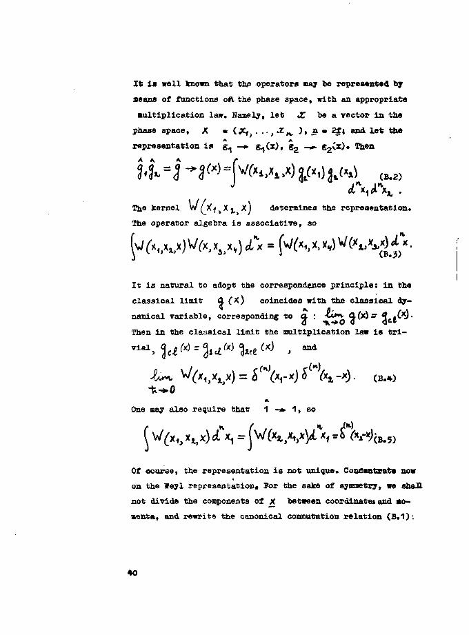
It ia well known that top operators may be represented by

oeans of functions oft the phase space, with an appropriate

multiplication law. Namely, let X be a vector in the

phase space, Л • {У~1) . ..

> 1

Л ), n • 2f j and let the

representation is g^ —» g^Cx), g2 —- g

2vx). Then

The kernel w / x ^ X j , * ) determines the representation.

The operator algebra is associative, so

Ic is natural to adopt the correspondence principle: in the

classical limit O. (*) coincides with the classical dy-

namical variable, corresponding to a : -t**»v Л{х)г JLift)-

Then in the classical limit the multiplication law is tri-

eOO , and

CB.4)

Л.

One may also require that

Of course, the representation is not unique. Concentrate now

on the Weyl representaCion, Рог the sake of symmetry, we shall

not divide the components of X between coordinates and mo-

menta, and rewrite the canonical commutation relation (B.1):

«here ^ ^ i e

* constant antisymmetric matrix (lnrer-

se to that of the fundamental symplectie fora). Define the

symmetric product ( 3^ ... *• ) by means of the generating

function

Z (VЧ,);Ш (B.7)

wlver« г к и a vector -frowt a "J.utl" spa.ee,the monomials (X

u ... X. ) form a complete basis

of the operator algebra* iny operator Q may be represen-

ted as a forml aeriested as a formal aeries

where <J f->)) axG t n e n

S "" number" totally symmetric ten-

sors» She Weyl representation is defined by means of this

decomposition:

V"**-Evidently, the correspondence is one-to-one. The Weyl rep-

resentation may be described in an equivalent form, nyiking

a direct use of the definition (B.7), and it was just the

original prescription [*3 1 • Consider the Fourier transform

(В.Ю)

л

The corresponding operator a is constructed by means ofa

41

л.the exponential operator XL :

Г,

How we are in position to find the kernel of the multi-

plication law Bq. (B.2). Note that in view of the commuta-

tor Sq. (B.6), the operators -12. (r) fora a protective group

B.12)

The following equalities are also useful:

r

(ВИЗа)

(ВИЗс)

Substituting the representation (B.11) and using the Fourier

trausiorm, inverse to (ВИО), one gets

ВИ4)

с в*

1 5 )

I.e. oi ia the matrix, inverse to a) . It ia

le that in case of one degree с ' freedon (n • 2) the bili-

near form in the exponential of Sq. (B.14) has a aiaple

geometrical meaning: it is proportional to the area of the

triangle with vertices (х^,х-,Хс) o n ^

в phase plane.

1 somewhat more familial? way to represent the operators

is to use their kernels, say, in the coordinate basis<

Ihe multiplication law is mueh simpler, than Eo.. (B.2), how-

ever, the correspondence to the classical mechanics is not

so transparent. To get a relation between the symbol and

the kernel one needs to calculate the kernel for the opera-

tor SL (r). Return to usual coordinates and momenta and

note that in view of Sq. (B.12)

It follows from (B.9) and (B.11) «hat

4In conclusion, mention two nice properties of the Weyl

symbols, that are generalized also to the Grassmann case.

first, the Hermifcean conjugation of the operators induces

the complex conjugation of symbols Й ~* %&*, Q —* Q QQ.

dSecond,

43

Hepresentation of quanta! operators by means of func-

tions in the phase space was developed by Weyl £43J and

figner [44 ] , and further investigated by Moyal [45] . Ge-

neralisation to infinite number of degrees of freedom and

to the Fermi case, as well as some proofs and details may

be found in the works by one ->f the authors [46,20J . A mo-

re recent paper o* this subject ia that by Schmuts [47J •

Appendix C. Representation of Green's Function by Means

of the Phase-Space Path Integral

Consider a classical mechanical system with a Hamilto-

nian H( J< ), where X_ is a vector from the phase space.

Write the classical action in the symmetric form. • £ •

(0.1)

where (H*Sl)s од - д£, the notation is used in Appendix

В (Sq. (B.15) ). Tula action appears in the phase space path

integral representation of the propagator (Green's operator^A

Let H be the Ramiltonian operator of the quantised

system; H( X ) is the Weyl symbol of H , and G(t) •

m exp (-it̂ -fc, ) is the proparator. Calculate the Weyl sym-

bol of G(t), i.e. a function G(j< ; t) on the phase space.

To this end Btart from an infinitesimal time interval £t .

Evidently

S3 1 - L at H/*v -> 1,- i4t Н{Х)/ь> ,

lor a finite £ the operator G(t) may be oaloulated by

means of the Uniting process, representing the step-by-

-step evolution of the system

Ы-+00

To get the symbol G( x; t) we apply the multiplication lav

(B.2) with the kernel (B.14) to the symbols G(x, t/H) gi-

ven by £q. (С.2Ч The result is

G(x;t)

where v s

j( . One may imagine that the system is

propagating in the phase space, being influenced by itb Ha-

miltonian at points ^^ and being observed at points X^ .

Formally, '&$. (0*4) is a representation of the propaga-

tor by means of a "double" continual integral J

J j p= J j- I (**) - H(

3)J dx }

t,

5 )

where the boundary condition j( (t) » X is implied. How-

ever, to evaluate this expression one should consider the

original form (C.4). The integral in Jf^ is Gaussian and

may be calculated exactly. Substitute « X y= "Hyf-iyt wh*-

re 2 J я ™ the new integration variables and the bilinear

form In the exponent has an extremum at /^ = it у • The

equations to determine U ^ are

(C.6)

*<*• s 111 , t<. = .X

Assume that N is an even number; then one gets

« ,

In the continual limit Sqa.(0.6) for "Ц are written ав

u . 1/2 y, u(0) . y(0), (0.9)

во that u( T ) * 1/2(y( Г ) + y(o) ), and

(оио)

where <^c/ i

fi the classical action defined by Бд. (С.1).

This form of the phase-space path integral is quite symmet-

ric) one does not need to distinguish between the coordina-

te and the momentum, noj* to prescribe that the trajectories

are piecewise linear in £ and piecewise constant in j> ,

as in the conventional approach (see the work by Garrod

). However, the exact meaning of the functional

is clear only before the limit H —»©0 and

is given by Bq. (C.8).

In some applications the representation (C.4) is more

useful than (C.8) or (C.10). For Instance, to get the Veyn-

man original path integral in the coordinate space one may

introduce the variables (p,q.) • y, (p , q ) • x, write

H(y) * p /2m + V(q) and integrate (C.%) first over p, then

over q and p . Consider now the isotrope harmonic os-

cillator

H(y) x k*i (0.11)

Integrating (С.4) over Vy we obtain

(СИ2)

wiiere 2y = «*у -Уу + , , £xkV/v*.eaSmwV iXter the in-

ogration over j^ у , 1 < М ^ Я the in-

takes the form

J-. -

t M+i b

while for the constants i, ы C,, ̂ f o U o w i l l g

recursive

relations hold

, . ^ „ . .- _ С0.14)

la the continual Halt, S->C , J* - A(Mt/H), CM •

»(£.*£ 5" ̂ " V 2 f(Mt/5), and the functions i.( ТГ ) and

f( T ) are obtained trom the differential equations

г

А(0) . О, »(0) . 1.

fham Green's function for the oscillator is

3.16)

Ipplying So.» (B.18), relating the symbol of an operator to

its matrix element, one can see that this result la in ac-

cordance with that given by Feynman [291 •

2b» phase-space path integrals were introduced by Jeyn-

шап [48J and dlaoussed in a number of works [49-517 • The

present exposition follows the work [ 20J .

48

H t f e t t n c » !

1. ?.A.Bere»in, "Ihe Method of Second Quantisation" (in

Russian), Sauka, Moscow, 1965» English transit Acad—ic

Press, Hew Xork, 1966

2. J.Raewuski, Tie Id Theory IIй, Illffe Books Ltd., Lo&-

don,1969

3. P.T.Matthews and A.Salam, 5uovo Cia., g (1955) i 120

4. J.L.Gervais and B.Sakita, Bucl.Phys., B64 (1971), 632

5. T.Iwasaki and K.Kikkawa, Phys.Rev., Ш (1973) 4*0

6. Tu.A. Golf and and E.P.Lichtman, JBTP Letters (USSR), 1£

(1971), *52

7. B*2umlno, in Proceedings of the X7XI International

Conference on High Energy Physics (London, July 1974).

Ed. J.R.Smith, Rutherford Laboratory, Chilton, Didcot,

p.1-254

3. J.I.Frenkel, Zeitschr. t. Physik J2 (4926), 247

9. J.I.Trenkel, "Electrodynamics" (in Russian), ORTI,

Moscow, 1934, p.401

10. A.O.Barut, "Electrodynamics and Classical Theory of

fields and Particles", W.Benjamin, N.T. 1964

11. A.J.Hanson and T.Regge, Ann.Phys. (H.T.) §2_ (1974),498

12 F.A.Berezin and G.I.Katx, liath.Sbomik (DSSR) 82. (1970)343

13. L.Corwin, I.He'eman, and S.Staeinberg, Hev.Mod.Phys.,

4Z (1975), 5*3,

14. ff.A.Berezin and M.S.Mariner, JSXP Letters (USSR) SI

(1975), 67815. J.Schwinger, Phil.Mag., 44 (1953),

16. J.L.Martin, Froe.Roy.Soc., A2ffl (1959), 556

17. B.S.de Witt, Bull.Aner.Fhys.Soc, 20 (1975), 70

18. A.M.Perelonov and V.S.Popov, Theor. Hath. Fhye. (USSH),

1 (1969), 360

19« P.A.M.Dirac, "The Principles of Quantum Mechanics",

The Clarendon Press, Oxfo-d, 1958

20. F.A.Beresin, m4eor. Math. Phys. (USSH) 6 (1971), 19*

21. I.M.Khalatnikov, JEEP (USSR) 28 (195*), 635

22. D.J.Candlin, Nuovo Cim., 4 (1956), 231

23. J.L.Martin, Proc. Roy.Soc, A251 (1959), 5*3

2*. F.A.Bere*in, Dokl. Akad. ETauk (USSR) 1^2 (1961), 311

25. L.Schulman, Phys.Rev., 17_6 (1968), 1558

26. V.Beiak, In t . J.Theor.Phys., 11. (197*)» 321

27. F.A.Beresin, "General Concept of Quantisation", Prep-

rint ITP-74-20B, Kiev, 197*; Comm.Math.Phye., 40 (1975),

153

28. J.Tarski, "Phase Spaces for Spin and their Applicabi-

lity", Preprint IC/7V129, ICIP, Trieste, 197*

29. R.P.Peynman and A.R.Hibbs, "Quantum Mechanics and Path

Insegrals", Mcdraw-aill Book Co., N.T., 1965

30. P.A.M.Dirac, "Lectures on Quantum Mechanics", Belfer

Graduate School of Science, Teshiva University, New

Tork, 196*

31. R.Casalbuoni, J.Gomis, and G.Longhi, Nuovo Cim., 2*A

(197*), 2*932. I.J.Jordan and N.Mukunda, Phys.Rev., 1^2 (1963), 18*2

33. L.Michel and A.S.Wightman, Phys.Rev., ̂ 8 (1955), 1190

3*. L.G.Suttorp and S.R.de Groot, NUOTO Cim., 65_A (1970),

2*5

35. J.H.Bllis, J.Phys., A2 (1970), 251; A*_ (197D, 583

50

36» V.Bargmtm, L.Michel, and T»l»9alagdl*

2 (1959). « 5

57. T.Bargumn and Ж.Р.Швпаг, I* oe. Vaftl.iead.Sel. USA,

34 (19M), 211

38. M.SJtariaoV, Aan.Phja., (Ж.1.) 4£ (1968), 357

39. J.Schwiaeer, РЬув.Нат., 8£ (195D. 91*« 21 (1953), 713

40. C.Rebbi, Ehjs.Hepta. 1 £ (197»), 1

41. R.Rajapaman, Ha78.Hepta. 1̂C (1975)* 227

42. J.R.ELauder, lan.Hiye. (H.T.) 11 (1960), 123

43. H.Weyl, Z.fb7S.. 46 (1927). 1 | "ttruppenthaepia mid

Quantasmeohaoik", S.Elrsel, Laipais. 1928

44. l.P.».isner, Hiye.RaT., 40 (1932), 749

45. J.B.Moyal, Егос. СавЬг. ail.Src, 4£ (1949:, 99

46. y.JL.Beresln, Proe. Hoaeow Math. Soc, 12 (1967). 117

(In Bnaalaxi)

47. «.Scbonta, Яоото Cia., 252 (1975). 337

48. B.IejBMtt, РЬув.Нвт., §1 (195D* 108

49. H.Dariea, Froe. Cambr. Phil.Soe., 52 (1963)» 147

50. C.Garrod, HeT.Mod.Ebje., jg (1966), 483*

51. L.D.Iaddear, The0r.Math.Pb7e. (USSR) 1 (1969), 3

52. D.T.TolkOT, S.7.Paletaiaak7. JSEP (USSR) 2Z (1959) .170.

Я

Работа поступила в ОНТИ 1 Д П - 1976г.

Подписано к печати Ю/Ш-76г. Т - 03270. Печ.л. 3,25.Формат 70x108 I/I6. Тираж 300 экз. Заказ 43. Цена 17 код.

Отдел научно-технической информации ИТЭФ, II7259, Москве