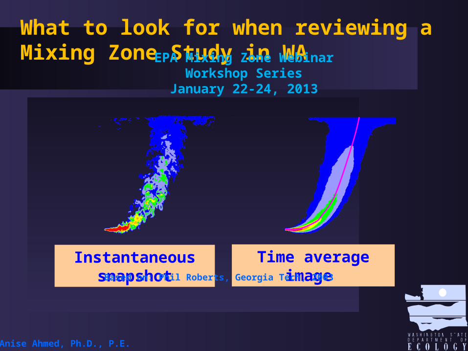
Instantaneous snapshot Time average image Based on: Phil Roberts, Georgia Tech, 2003

What to look for when reviewing a Mixing Zone Study in WA EPA Mixing Zone Webinar Workshop Series

January 22-24, 2013

Anise Ahmed, Ph.D., P.E.

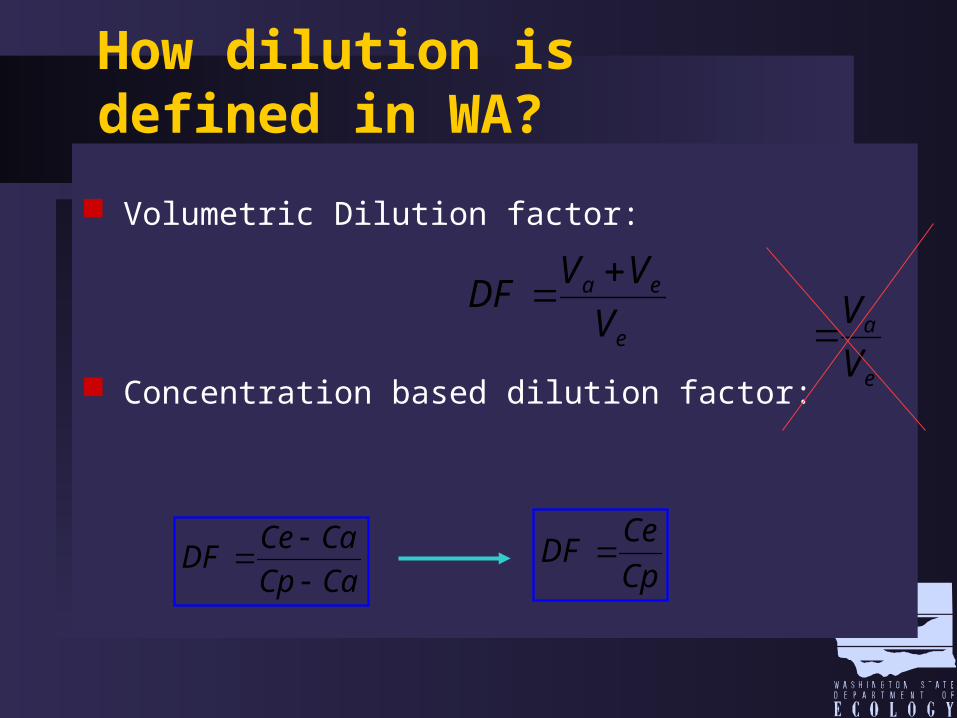
Volumetric Dilution factor:

Concentration based dilution factor:

How dilution is defined in WA?

CaCp

CaCeDF

e

ea

V

VVDF

Cp

CeDF

e

a

V

V

• Apply AKART prior to mixing zone authorization • Maximum size of mixing zone• Minimize mixing zones• Must prove no environmental harm• Consider critical conditions

Mixing Zones in WA (WAC-173-201A-400)

Other Mixing zone regulations

Overlapping mixing zones Extended mixing zones Mixing zones for stormwater Mixing zones for CSOs

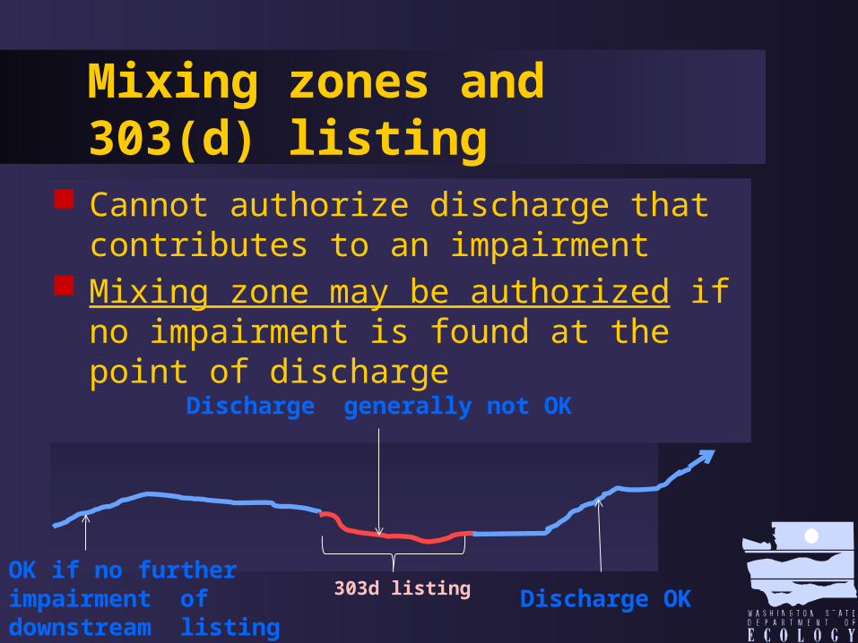
Mixing zones and 303(d) listing

Cannot authorize discharge that contributes to an impairment

Mixing zone may be authorized if no impairment is found at the point of discharge

Discharge OK

Discharge generally not OK

OK if no further impairment of downstream listing 303d listing

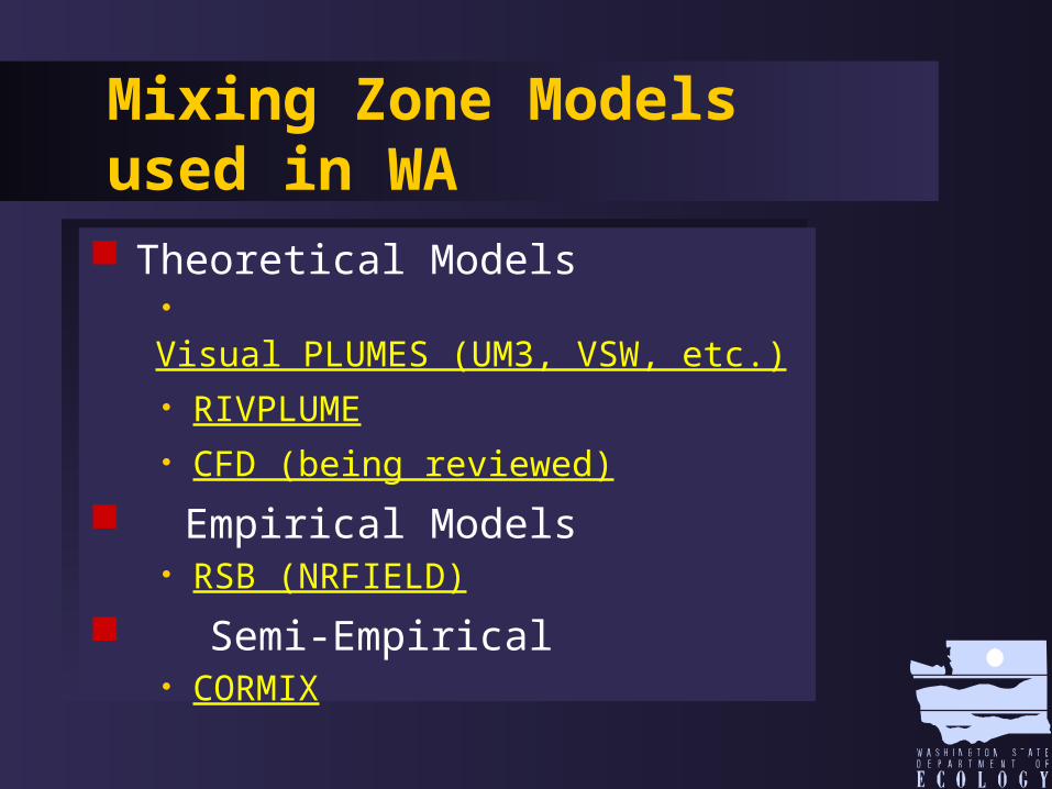
Mixing Zone Models used in WA

Theoretical Models• Visual PLUMES (UM3, VSW, etc.)• RIVPLUME• CFD (being reviewed)

Empirical Models• RSB (NRFIELD)

Semi-Empirical• CORMIX

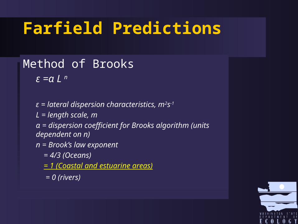
Farfield Predictions

Method of Brooksε =α L n

ε = lateral dispersion characteristics, m2s-1

L = length scale, m

α = dispersion coefficient for Brooks algorithm (units dependent on n)

n = Brook’s law exponent

= 4/3 (Oceans)

= 1 (Coastal and estuarine areas)

= 0 (rivers)

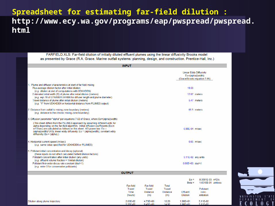
Spreadsheet for estimating far-field dilution : http://www.ecy.wa.gov/programs/eap/pwspread/pwspread.html

http://www.ecy.wa.gov/programs/eap/mixzone/mixzone.html

The End

Mixing Zones Guidance in WA

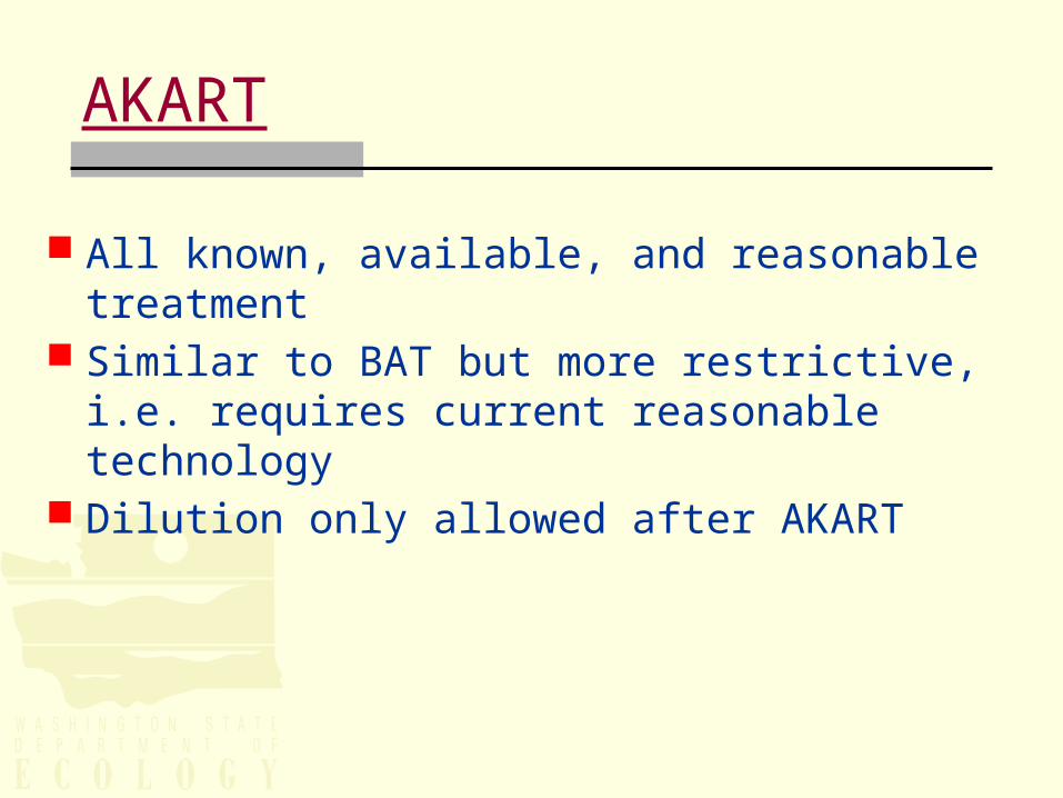
AKART

All known, available, and reasonable treatment Similar to BAT but more restrictive, i.e. requires

current reasonable technology Dilution only allowed after AKART

Maximum Size: Streams

Hydraulic Limitation Can use only max stream flow of 25% 7Q10

Distance Limitation

Chronic Zone =300 feet + d

Acute Zone = 10% of Chronic

25%W

diffuser

W

d = depth of diffuser at 7Q10W = width of stream at 7Q10

NPDES

NPDES

Q

QQDF

107*25.0max

100 ft

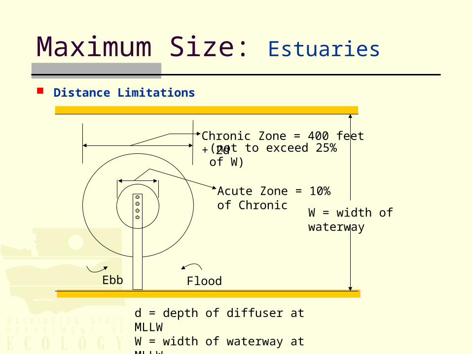
Maximum Size: Estuaries

Distance Limitations

W = width of waterway

Chronic Zone = 400 feet + 2d

Acute Zone = 10% of Chronic

d = depth of diffuser at MLLWW = width of waterway at MLLW

(not to exceed 25% of W)

Ebb Flood

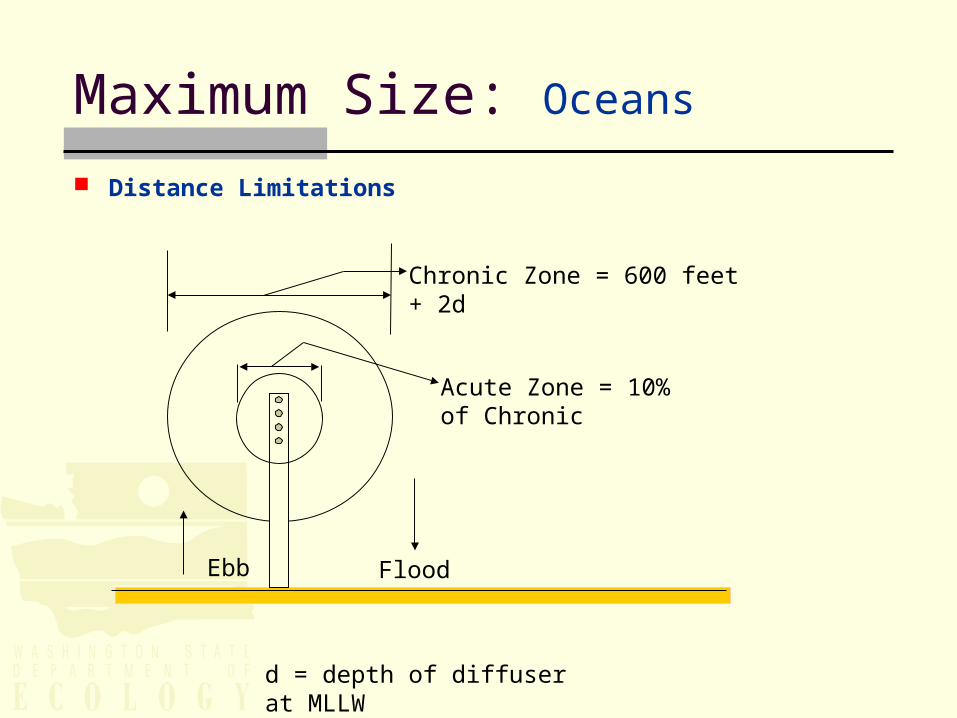
Maximum Size: Oceans

Distance Limitations

Chronic Zone = 600 feet + 2d

Acute Zone = 10% of Chronic

d = depth of diffuser at MLLW

Ebb Flood

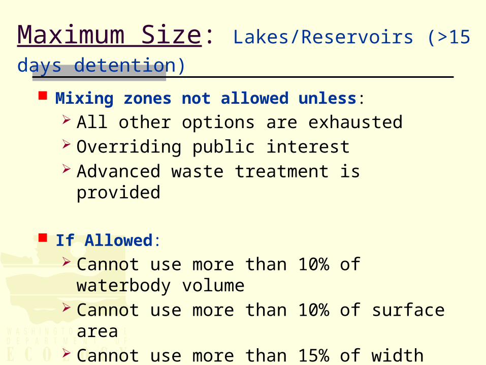
Maximum Size: Lakes/Reservoirs (>15 days detention)

Mixing zones not allowed unless: All other options are exhausted Overriding public interest Advanced waste treatment is provided

If Allowed: Cannot use more than 10% of waterbody

volume Cannot use more than 10% of surface area Cannot use more than 15% of width of

waterbody.

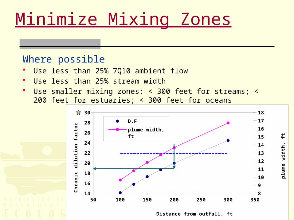
Minimize Mixing Zones

Where possible Use less than 25% 7Q10 ambient flow Use less than 25% stream width Use smaller mixing zones: < 300 feet for streams; < 200 feet for

estuaries; < 300 feet for oceans

50 100 150 200 250 300 35014

16

18

20

22

24

26

28

30

8

9

10

11

12

13

14

15

16

17

18

D.Fplume width, ftplume width allowed, ft

Distance from outfall, ft

Ch

ron

ic d

iluti

on f

acto

r

plu

me

wid

th, f

t

No environmental harm

No loss of sensitive or important habitat, No interference with existing or

characteristic uses of the waterbody No resulting damage to the ecosystem No adverse public health affect

Critical Conditions

Flow and Concentration Ambient flow Effluent flow Ambient/Effluent concentrations

Depth Stratification Dilution type

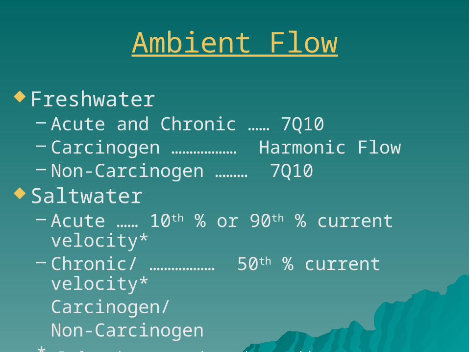
Ambient Flow

Freshwater– Acute and Chronic …… 7Q10– Carcinogen ……………… Harmonic Flow– Non-Carcinogen ……… 7Q10

Saltwater– Acute …… 10th % or 90th % current velocity*– Chronic/ ……………… 50th % current

velocity*Carcinogen/Non-Carcinogen

* Evaluated over a spring and neap tide

Effluent Flow

Acute … highest daily Qmax in last 3 years

Chronic/Non-Carcinogens … highest monthly Qavg

in last 3 years Carcinogens … Annual Average Flow Stormwater (Western WA):

– Acute …… 1-hour peak flow from 2-yr 6-hr storm event– Chronic ..... Average flow from 2-yr 72-hr storm event

Intermittent flow: – Estimate DF using Qmax

– Increase DF by (Q1-hr avg/Qmax) for acute

– Increase DF by (Q4-day avg/Qmax) for chronic

For Estimating Volumetric Dilution Factor

Ambient Concentration:– Assume zero when no reflux– If reflux is present use reflux as ambient

Effluent Concentration: – Assume 100% or 100 ppm

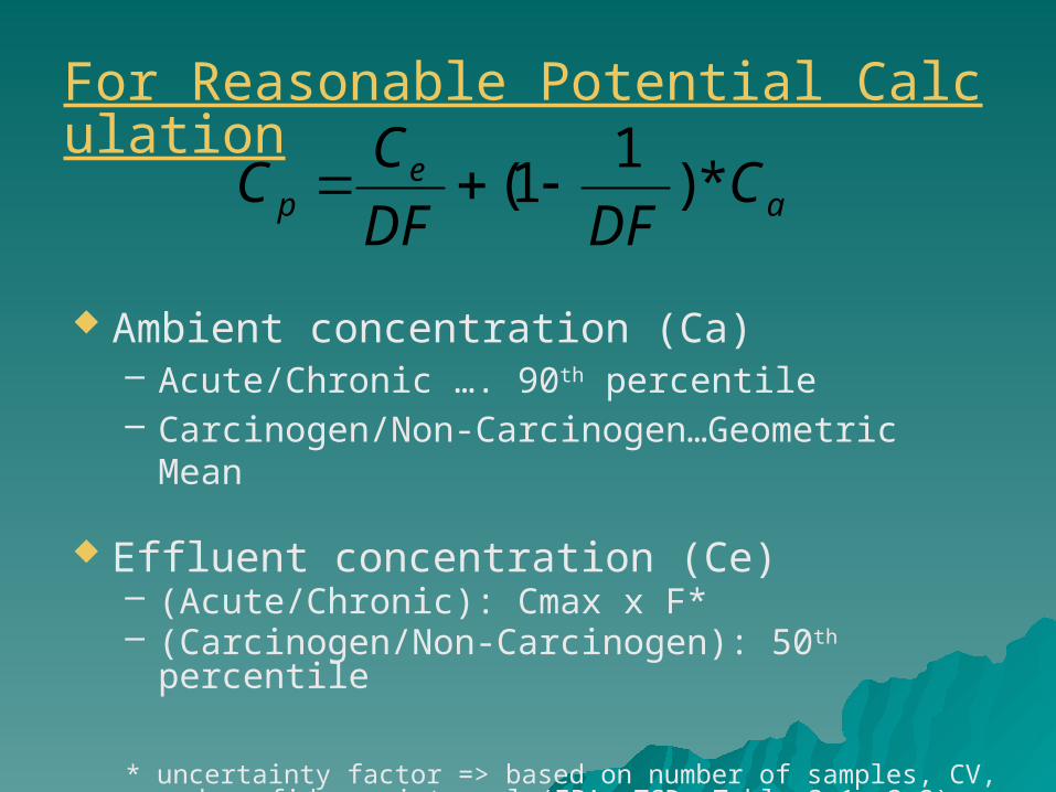
For Reasonable Potential Calculation

Ambient concentration (Ca)– Acute/Chronic …. 90th percentile– Carcinogen/Non-Carcinogen…Geometric Mean

Effluent concentration (Ce)– (Acute/Chronic): Cmax x F*– (Carcinogen/Non-Carcinogen): 50th percentile

* uncertainty factor => based on number of samples, CV, and confidence interval (EPA, TSD, Table 3-1, 3-2)

ae

p CDFDF

CC *)

11(

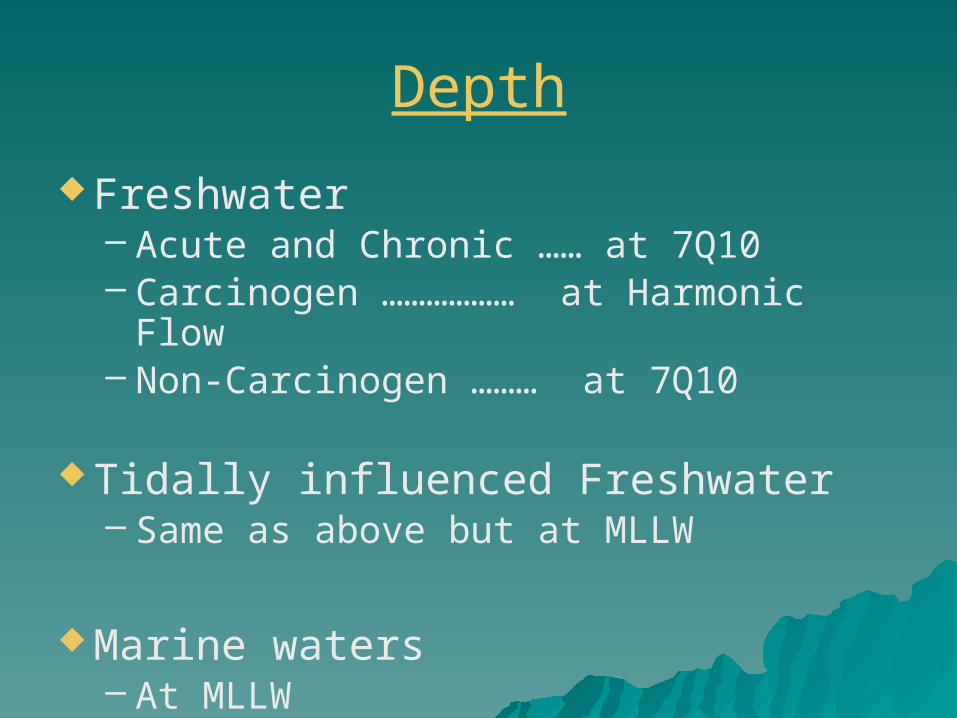
Depth

Freshwater– Acute and Chronic …… at 7Q10– Carcinogen ……………… at Harmonic

Flow– Non-Carcinogen ……… at 7Q10

Tidally influenced Freshwater– Same as above but at MLLW

Marine waters– At MLLW

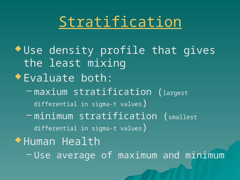
Stratification

Use density profile that gives the least mixing

Evaluate both:– maxium stratification (largest differential in sigma-

t values)– minimum stratification (smallest differential in

sigma-t values) Human Health

– Use average of maximum and minimum

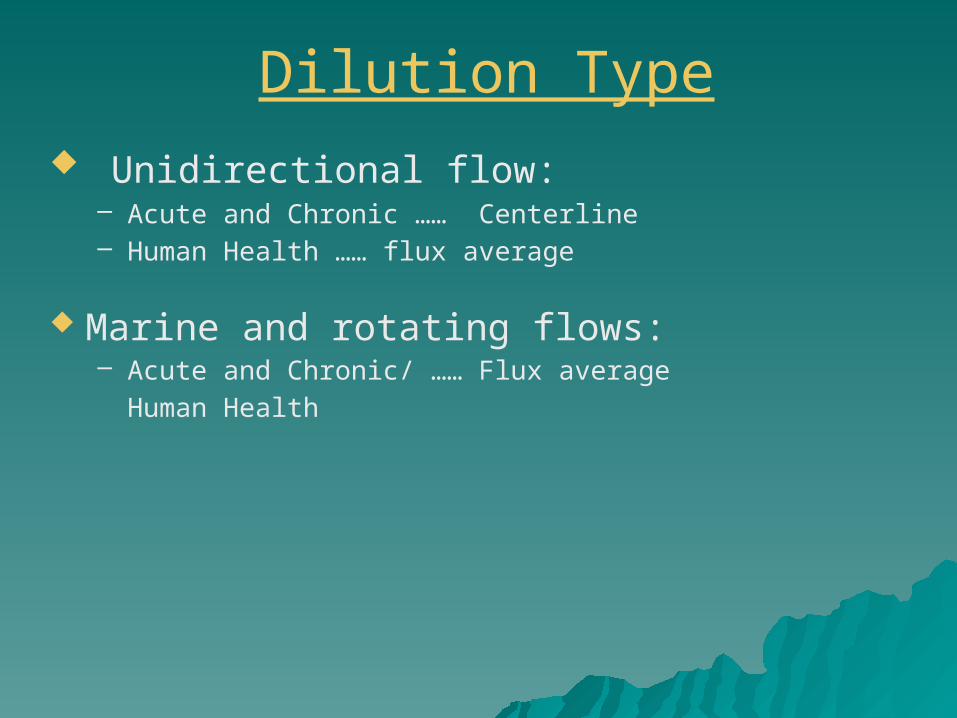
Dilution Type Unidirectional flow:

– Acute and Chronic …… Centerline– Human Health …… flux average

Marine and rotating flows: – Acute and Chronic/ …… Flux average

Human Health

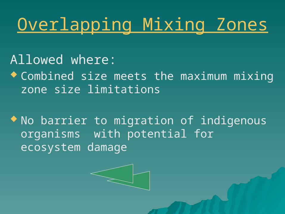
Overlapping Mixing Zones

Allowed where: Combined size meets the maximum mixing

zone size limitations

No barrier to migration of indigenous organisms with potential for ecosystem damage

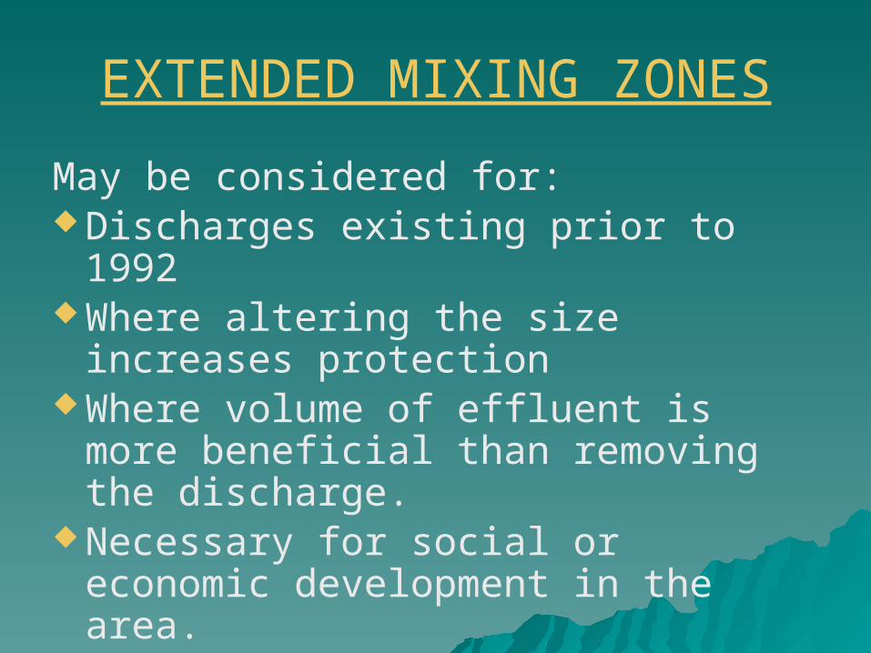
EXTENDED MIXING ZONES

May be considered for: Discharges existing prior to 1992 Where altering the size increases

protection Where volume of effluent is more

beneficial than removing the discharge.

Necessary for social or economic development in the area.

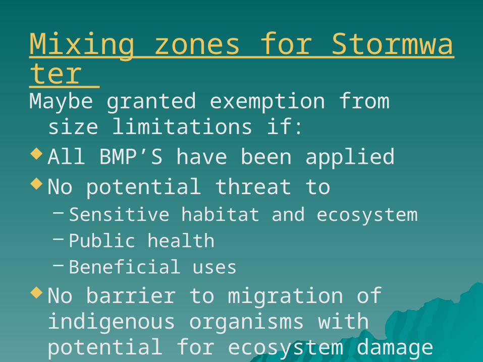
Mixing zones for Stormwater

Maybe granted exemption from size limitations if:

All BMP’S have been applied No potential threat to

– Sensitive habitat and ecosystem– Public health– Beneficial uses

No barrier to migration of indigenous organisms with potential for ecosystem damage

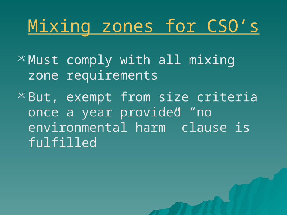
Mixing zones for CSO’s

• Must comply with all mixing zone requirements

• But, exempt from size criteria once a year provided “no environmental harm” clause is fulfilled

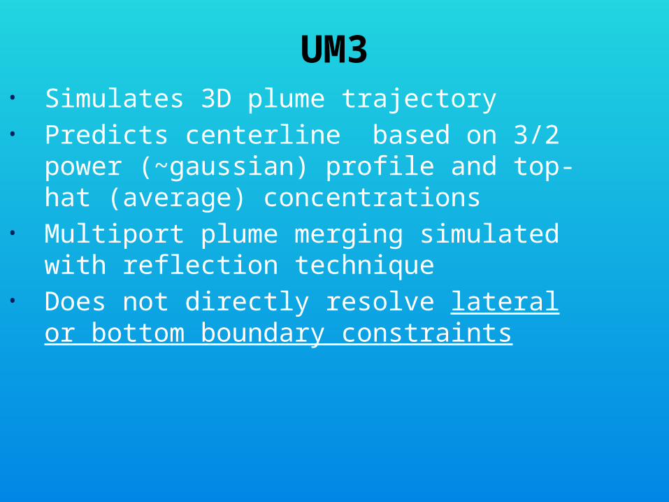
UM3• Simulates 3D plume trajectory• Predicts centerline based on 3/2 power

(~gaussian) profile and top-hat (average) concentrations

• Multiport plume merging simulated with reflection technique

• Does not directly resolve lateral or bottom boundary constraints

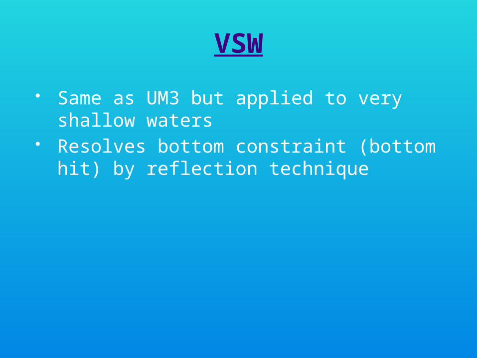
VSW

Same as UM3 but applied to very shallow waters

Resolves bottom constraint (bottom hit) by reflection technique

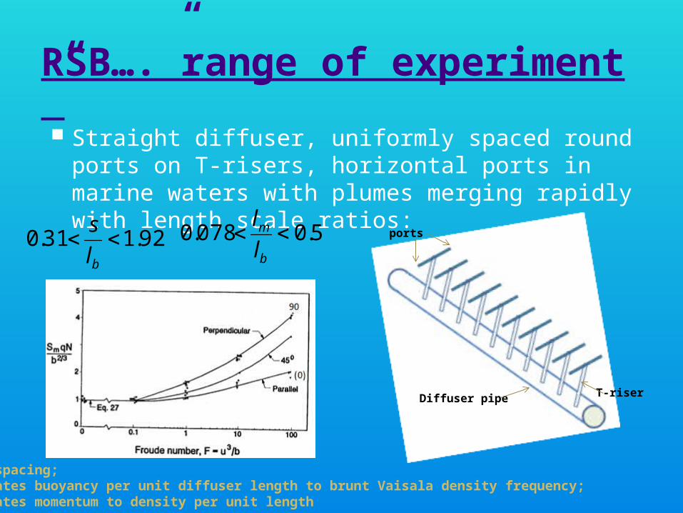
RSB….”range of experiment” Straight diffuser, uniformly spaced round ports on

T-risers, horizontal ports in marine waters with plumes merging rapidly with length scale ratios:

5.0078.0 b

m

l

l92.131.0

bl

s

S = port spacing; lb = relates buoyancy per unit diffuser length to brunt Vaisala density frequency; lm = relates momentum to density per unit length

Diffuser pipe T-riser

ports

CORMIX

CORMIX 1 single port positive/neutral buoyant discharges

CORMIX 2 multiport positive/neutral buoyant discharges Uses “equivalent slot diffuser” May need CORMIX1 if plume details near each

port are desired CORMIX 3 buoyant surface discharge

RIVPLUME (based on Fischer et al. 1979)

Single port, short diffuser, or bank discharge

Plume completely and rapidly vertically mixed within the acute zone. So a 2-D model

Uses mean cross-sectional velocity

It incorporates boundary effects of shoreline through superposition

Cannot model ambient density stratification, dense plumes or tidal buildup

Available at the following site:http://

www.ecy.wa.gov/programs/eap/pwspread/pwspread.html

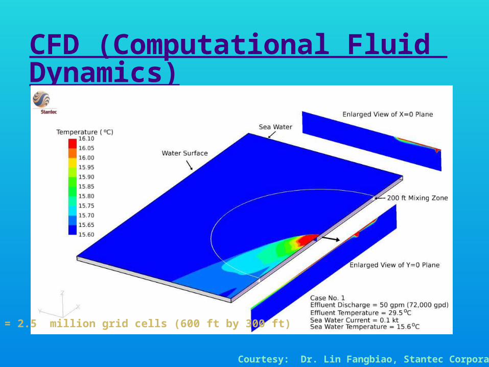
CFD (Computational Fluid Dynamics)

Mesh = 2.5 million grid cells (600 ft by 300 ft)

Courtesy: Dr. Lin Fangbiao, Stantec Corporation