Lawre

nce

Liverm

ore

National

Labora

tory

UCRL-ID-133563

Innovative Uses for Conventional Radiation Detectors via Pulse Shape Analysis

J. KammeraadD. Beckedahl

J. BlairA. Friensehner

G. Schmid

March 3, 1999

This is an informal report intended primarily for internal or limited external distribution. The opinions and conclusions stated are those of the author and may or may not be those of the Laboratory.Work performed under the auspices of the U.S. Department of Energy by the Lawrence Livermore National Laboratory under Contract W-7405-ENG-48.

DISCLAIMER

This document was prepared as an account of work sponsored by an agency of the United StatesGovernment. Neither the United States Government nor the University of California nor any of theiremployees, makes any warranty, express or implied, or assumes any legal liability or responsibility forthe accuracy, completeness, or usefulness of any information, apparatus, product, or process disclosed,or represents that its use would not infringe privately owned rights. Reference herein to any specificcommercial product, process, or service by trade name, trademark, manufacturer, or otherwise, doesnot necessarily constitute or imply its endorsement, recommendation, or favoring by the United StatesGovernment or the University of California. The views and opinions of authors expressed herein donot necessarily state or reflect those of the United States Government or the University of California,and shall not be used for advertising or product endorsement purposes.

This report has been reproduceddirectly from the best available copy.

Available to DOE and DOE contractors from theOffice of Scientific and Technical Information

P.O. Box 62, Oak Ridge, TN 37831Prices available from (423) 576-8401

Available to the public from theNational Technical Information Service

U.S. Department of Commerce5285 Port Royal Rd.,

Springfield, VA 22161

Innovative Uses for Conventional Radiation Detectors via Pulse Shape Analysis

Final Report 97-ERD-017

March 3, 1999

J. Kammeraad, D. Beckedahl, J. Blair, A. Friensehner, and G. Schmid

1. Introduction

It is well known [1,2] that the leading edge of γ-ray signals from a

semiconductor detector depends upon the particulars of the γ-ray interaction and

the detector itself. The incident γ-ray interacts at one or more locations in the

detector, creating electron-hole pairs that drift under the influence of the

imposed electric field to their respective electrodes. The resulting current

depends upon the number of charge carriers, the local electric field, and the

charge carrier drift velocity.

In most applications, only a measure of the total energy deposited by the

γ-ray is needed. Optimum energy resolution is obtained by shaping the signal,

which strongly filters out the variations in the leading edge of the signals. In this

project we have shown that by properly recording the signals from a cylindrical

high purity germanium (HPGe) detector and utilizing pulse shape analysis, one

can obtain the distribution of the deposited energy as a function of the radial

coordinate in the detector. In this paper we present predicted and measured

position-dependent detector responses, a maximum likelihood approach for

accurately determining the radial energy deposition, and a least squares

approach for determining the radial energy deposition approximately and

2

rapidly enough for real-time applications in Compton suppression. The position

resolution that can be obtained in this process depends upon the spectral

properties of the electronic noise. We discuss the uncertainties that result from

the noise, and show that excellent position resolution can be expected. We also

discuss how this kind of signal processing can be extended with segmented

HPGe detectors to obtain all three coordinates of γ-ray interactions, allowing the

development of a high efficiency Compton “camera” for γ-ray imaging.

Analog and digital pulse shape analysis with Ge detectors has been

utilized in many instances to optimize detector performance by deriving

additional information from pulses beyond a measure of the peak height or

integral. Applications include discrimination between γ-ray, neutrons, and

protons [3], identification of beta decays in the detector [4-6], rejection of

Compton escape events [7-11], reduction of γ-ray Doppler broadening effects

[12], and adaptive shaping to enhance energy dispersive spectroscopy [13].

Signal processing techniques are also important in the development of detectors

for basic nuclear physics research, such as the proposed Gamma-Ray Energy

Tracking Array (GRETA) [14].

2. Determination of the radial position of gamma-ray interactions in a

cylindrical HPGe detector

For the energy range of interest (E<2 MeV), the ranges of electrons

generated by γ-ray interactions in germanium are small (less than 2 mm). Thus to

a good approximation, one can consider the signal, S(t), from a multiple-

interaction γ-ray event to be the sum of the signals, Si(t), resulting from the

3

energy deposited at the location of each γ-ray Compton/photoelectric

interaction:

S t S tii

m

( ) ( ),==∑

1

(1)

where m is the number of Compton/photoelectric interactions in the event. In a

coaxial detector each Si(t), can be expressed as Si(t), =EiK(t,ri) , where Ei is the

energy deposited at interaction i, and K(t,ri) is the response of the detector to an

impulse of unit energy at radius ri . Then Equation (1) becomes:

S t E K t r E a K t ri ii

m

i ii

m

( ) ( , ) ( , )= == =∑ ∑

1 1

(2)

where E is the total energy deposited in the γ-ray event and ai is the fractional

energy deposited at interaction i. For conventional HPGe detectors, the goal is to

determine the coefficients ai for each measured signal, thus providing the energy

deposition as a function of r. The ability to do this in a manner that is useful to

various detection applications depends upon a good understanding of the

functions K (t, ri), adequate radial resolution (which depends upon both signal

and noise properties), and a rapid numerical algorithm to invert Equation (2).

2.1 Predicted and measured signals as a function of radius.

Because charge carrier trapping is negligible in high purity germanium,

the leading edge signal shape depends only upon the position at which the

charge carriers are generated, the local electric field along their drift paths, and

their drift velocity. Figure 1 shows several theoretical signals from single

interactions in a coaxial detector as a function of radial position. (In these

4

calculations we have assumed that the charge carrier velocity is saturated and

constant throughout the detector.)

The signals, which represent the induced charge due to electron/hole

current, have distinctly different shapes. Each signal changes smoothly as the

electrons and holes move into regions of higher and lower electric field

respectively. Discontinuities in the derivative of each signal occur at points in

time which correspond to the arrival of a group of charge carriers at an electrode.

We measured the impulse response functions K(t,ri) with a closed-end,

coaxial, n-type, high purity germanium (HPGe) detector with an inner radius of

0.5 cm, an outer radius of 2.5 cm, and length of 5 cm. The closed end is 9mm

thick. The bias voltage applied to the detector is -3000 volts, which is sufficiently

high that the drift velocities of the charge carriers can be taken to be saturated

and constant over most of the volume of our detector, as described below.

Signals from the detector preamplifier were processed in two parallel

paths. In one path the conventional signal shaping and pulse height

measurement was performed. In the other path the signal was compensated,

amplified, and recorded in digital form. The compensating circuit, consisting of

wide-bandwidth amplifiers and RC filters, was selected to extend the system

bandwidth to 25 MHz and to condition the noise to make it into “white noise”.

As described in Section 2.2, this step is necessary in order to use a least-squares

approach when solving for the coefficients ai in Eq 2. Two different types of

compensating circuits were used in this project. In the initial circuit we used RC

filters that differentiated the signals in order to make the discontinuities in slope

more apparent. Although this approach is useful for purposes of visualization, it

is not the optimum approach. Later, we used filters that compensated for the

5

high frequency loss of the preamplifier, which allowed a more accurate

determination of the coefficients ai for each measured signal. The signals were

recorded every nanosecond with 8 bit accuracy with a Tektronix DSA 602

digitizer, and recorded in event mode along with the usual measurement of the

pulse height of the shaped signal. The event mode data were later analyzed on a

Macintosh 8100 computer using LabVIEW .

We obtained the radial response functions K(t,r) by two methods: direct

measurement using a highly collimated γ-ray source; and convolution of the

idealized signals (as in Fig. 1) with the preamplifier frequency response. The

measurement of the preamplifier frequency response is described in Section 2.2.

Measurements of detector response functions K0(t,r) were obtained using a

2-inch long, 1-mm diameter Au collimator in a 6-inch long heavymet holder that

attenuated transmitted γ-rays. The collimator was carefully aligned with the

detector and positioned such that the umbra was centered on the radial zone of

interest. A Cs-137 check source was placed on the collimator axis, and the

signals were gated to record only those events in which the deposited energy

was between 0.42 MeV and 0.47 MeV; i.e., the event was near the “Compton

edge”. This energy was chosen because the probability of a single interaction is

relatively high in this region. Measurements were obtained at 20 equally spaced

locations along a detector radius, each 1 mm apart.

Even with gating and tight collimation, most measured signals did not

represent single interactions at the target radii. Signals were accepted or rejected

according to the following method. Each signal Sj(t,r) measured at radius r was

compared with the signal Kp(t,r,ve,vh) predicted with specific values of the

6

electron and hole velocities ve and vh. We kept those signals that satisfied the

following equation:

S t r c K t r v v dtj j j p e h

T

( , ) ( , , , )− − ≤∫ τ α0

2

, (3)

where T = 1024 ns, and the time shift τ and the normalization constant cj were

chosen to minimize the integral. Using α= 5 x 10-5, we averaged the signals that

satisfied Equation (3) in order to obtain the measured pulse response function at

each radial location. The number of signals in the average varied as a function of

position from about 50 in the inner zones to about 250 in the outer zones.

The radial responses obtained by the two methods are very similar to each

other, as shown in Figure 2 for one response function. The responses obtained

by convolution of the ideal signals with the system response were slightly

modified, by adjusting the velocities of the charge carriers, to fit the width of the

responses obtained by the collimation method. By using an electron drift

velocity of 9.5 x 106 cm/s and hole drift velocity of 7.5 x 106 cm/s, we were able

to obtain good agreement between the responses obtained by both methods for

all ten radial zones with our detector.

The high degree of similarity between the two curves in Figure 2 is very

encouraging. It implies that for the coaxial portion of the detector the signals can

be understood in terms of very simple quantities: the electric field, the energy

deposited (i.e., the number of charge carriers generated), and the charge carrier

velocities. As a result, the techniques described in this report can probably be

extended to other HPGe detectors in a straightforward manner.

7

The closed end (non-coaxial or “quasi-planar” region) of the detector

introduces a difficulty, because γ-rays that interact in this region generate signals

that are not well fit by Equation (2). In principle one could measure an additional

set of response functions which depend upon two cylindrical coordinates, r and

z, taking into account the possibility that drift velocities may vary with position

in this region. This approach adds significant complexity to the inversion

process. Alternatively, one could treat the signals that arise from an interaction in

the closed end by another strategy, such as rejecting them or counting them in a

separate spectrum.

2.2 Maximum likelihood approach

The goal is to accurately determine, from observed pulse shapes, the

radial positions and energies of the individual γ-ray interactions. If the pulse

shapes were recorded with perfect accuracy, one could calculate the parameter

values (Ei and ri) in equation (2) that give equality. Fortunately, there is only one

solution to this problem. However, the signals are not recorded with perfect

accuracy. They are corrupted by electronic noise from the measurement system.

The noise is significant, and its magnitude has already been reduced to nearly

the lowest practical level. This being the case, it is desirable to estimate the

unknown parameter values in a manner that makes good use of the statistics of

the noise.

We have chosen to use maximum-likelihood (ML) estimates for the

unknown parameters. Chapter 7 of [15] and section 2.4.2 of [16] explain why this

8

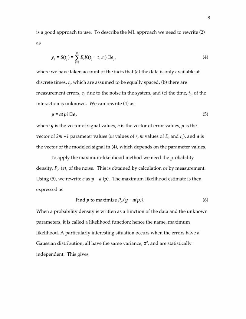
is a good approach to use. To describe the ML approach we need to rewrite (2)

as

y S t E K t t r ej j i j ii

m

j= = − +=∑( ) ( , )0

1

, (4)

where we have taken account of the facts that (a) the data is only available at

discrete times, tj, which are assumed to be equally spaced, (b) there are

measurement errors, ej, due to the noise in the system, and (c) the time, t0, of the

interaction is unknown. We can rewrite (4) as

y a p e= +( ) , (5)

where y is the vector of signal values, e is the vector of error values, p is the

vector of 2m +1 parameter values (m values of r, m values of E, and t0), and a is

the vector of the modeled signal in (4), which depends on the parameter values.

To apply the maximum-likelihood method we need the probability

density, PN (e), of the noise. This is obtained by calculation or by measurement.

Using (5), we rewrite e as y – a (p). The maximum-likelihood estimate is then

expressed as

Find to maximize p y a pPN ( ( )).− (6)

When a probability density is written as a function of the data and the unknown

parameters, it is called a likelihood function; hence the name, maximum

likelihood. A particularly interesting situation occurs when the errors have a

Gaussian distribution, all have the same variance, σ2, and are statistically

independent. This gives

9

P e e ee

e

N nj

j

n

n

jj

n

( , ,... ) exp

exp/

1 2 2

2

21

2 2

22

1

1

2 2

21

2

= −

= ( ) −

=

−

=

∏

∑

πσ σ

πσσ

. (7)

Rewriting ej in (7) as a function of the data and the unknown parameters and

realizing that maximizing (7) is equivalent to minimizing the summation in the

exponent, we obtain

Find to minimize p p( ( )) .y aj jj

n

−=∑ 2

1

(8)

This is a simple non-linear-least-squares problem, which can be numerically

solved [17, pp. 681-688].

For this special case the maximum-likelihood estimate reduces to the

least-squares estimate. Our approach is to preprocess the data in such a way that

the least-squares estimate always yields a maximum-likelihood estimate. The

conditions required for this are that the noise samples be Gaussian, have equal

variance, and be statistically independent. For a well-constructed system, the

errors are due to thermal noise being passed through a linear, time-invariant

system. This fact guarantees [18, p. 189] that the error samples are Gaussian and

have equal variance. However, the errors will not normally be statistically

independent.

The condition for the errors to be statistically independent is that the noise

must be white [18, p. 145-155]. This means that if we can force the noise to be

white, without increasing its magnitude relative to the signal, the maximum-

likelihood problem will reduce to the least-squares problem. We accomplish this

by measuring the power spectrum of the noise and designing a filter to convert

10

this spectrum to white. We then apply this filter to the signals that are recorded.

For this to work properly, the model signals in (2) have to be the signals that

have already been passed through the filter. The filter can be constructed as an

analog filter that is applied to the signals before they are digitized, a digital filter,

which is applied after the signals are digitized, or a combination of the two.

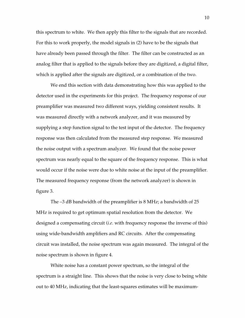
We end this section with data demonstrating how this was applied to the

detector used in the experiments for this project. The frequency response of our

preamplifier was measured two different ways, yielding consistent results. It

was measured directly with a network analyzer, and it was measured by

supplying a step function signal to the test input of the detector. The frequency

response was then calculated from the measured step response. We measured

the noise output with a spectrum analyzer. We found that the noise power

spectrum was nearly equal to the square of the frequency response. This is what

would occur if the noise were due to white noise at the input of the preamplifier.

The measured frequency response (from the network analyzer) is shown in

figure 3.

The –3 dB bandwidth of the preamplifier is 8 MHz; a bandwidth of 25

MHz is required to get optimum spatial resolution from the detector. We

designed a compensating circuit (i.e. with frequency response the inverse of this)

using wide-bandwidth amplifiers and RC circuits. After the compensating

circuit was installed, the noise spectrum was again measured. The integral of the

noise spectrum is shown in figure 4.

White noise has a constant power spectrum, so the integral of the

spectrum is a straight line. This shows that the noise is very close to being white

out to 40 MHz, indicating that the least-squares estimates will be maximum-

11

likelihood estimates. The noise power has been converted from volts squared to

MeV squared to correspond to the units we are using for the signals. The noise

density (the slope of the straight line) is 3.6X10-7 MeV2/MHz.

2.3 Theoretical limits in radial resolution due to noise

Using the measured noise intensity and the impulse response, one can

calculate the uncertainty, due to noise of the least-squares estimates of the

unknown parameters. We assume we have measurements satisfying equation

(4) and that the errors ej are independent and have standard deviation, σ, given

by

σ 2

2= I

t∆, (9)

where I is the noise intensity in Mev2/MHz, and ∆t is the time between samples

in µS. We have found that the data in the frequency range between 1 MHz and

25 MHz control the results, so if the noise is not perfectly white, its intensity in

this 1 to 25 MHz range should be used. The measured value for the system on

which we did our experiments was I = 3.6 X 10-7. The derivation of equation (9)

is given in [19].

The parameter values determined by the least-squares solution (6) will

contain a random error due to the influence of the noise. This error will have a

mean value of zero and a standard deviation that can be calculated. For this end

we need the sensitivity matrix, S, which, using the compact notation of (5), is

given by

Sap

= =∂∂

∂∂

, or Sapij

i

j

. (10)

12

Each column of this matrix is the change in the signal due to a unit change in the

corresponding parameter value. In [19] it is shown that the covariance matrix for

the errors in the unknown parameters is given by

C S S= ( )−σ 2 1T . (11)

The standard deviation for the ith parameter is given by

σ i iiC= . (12)

The results of these calculations for some specific situations are given in the next

section.

2.4 Prediction of attainable position resolution in r for single interactions

The theory of the last section was used to predict the attainable resolution

in the r variable for the detector used in our experiments. Noise-free signals

were predicted for our detector by Kai Vetter at Lawrence Berkeley National

Laboratory. The predictions were normalized to correspond to a single

interaction of 1 MeV. Electronic noise was taken into account using a noise

model that was 20% smaller (rms) than that shown in figure 4 (based on

measurements obtained with a previous version of the system). Figure 5 shows

the resulting rms error for the position resolution in mm as a function of r and z..

The resolution is inversely proportional to the interaction energy, so the error for

a 100-keV interaction would be ten times larger. If the noise levels shown in

figure 4 had been used in the calculation, the results would be 20% larger.

Note that the attainable radial position resolution is degraded in the non-

coaxial region as one would anticipate. There is also a region of somewhat

degraded radial position resolution in the portion of the coaxial region where the

13

drift times of the electrons and holes are approximately equal. While these

results take into account the effects of the variations in expected signal shapes

and electronic noise, they do not include the effects of finite electron range. (For

electron energies greater than about 250 keV the mean range in germanium is

greater than the predicted achievable radial position resolution.) Various sources

of possible systematic error, such as unknown detector non-uniformities, would

also degrade the position resolution. Nevertheless, these results are very

encouraging. They indicate that with care one should be able to obtain radial

position resolutions better than 1 mm over a large volume of the detector for the

energy range of interest.

3.0 Compton suppression via pulse shape analysis

The suppression of Compton background in γ-ray spectra is usually

performed by surrounding the primary detector (e.g., a Ge crystal) with a

secondary detector (e.g., BGO annulus) operated in anti-coincidence mode.

Unfortunately, the large size, weight, and cost of such a system can offset

expected benefits, especially for measurements performed in the field. For this

reason, a Compton suppression technique based only on details of the charge

pulse shape seems attractive.

Recent efforts to apply Ge detector pulse shape analysis (PSA) to

Compton suppression [7-11] have focused on general characteristics of the

charge pulse shape (rise-time, single-site vs. multiple-site shape, etc.). In this

project we developed and tested a more fundamental approach based on a

complete unfolding of the charge pulse shape into discrete components

associated with individual γ-ray interactions. This approach allows the

14

application of an algorithm that favorably rejects Compton escape events. Our

algorithm was chosen to allow for discrimination on both single-site and

multiple-site escape events. This differs from the algorithms of [10-11] that were

designed to reject only single-site events. Below and in [20] we present the details

of our algorithm along with experimental results from a real-time

implementation on a 5cm x 5cm HPGE detector.

The approach used for Compton suppression was to estimate what

fraction of the energy deposited in the detector by a photon was deposited in a

single interaction. If this fraction exceeds a certain value (which depends on the

total deposited energy), the signal is assumed to be an escape event rather than a

full-energy event. Using the least-squares fitting method of Section 2.2 we can

determine the number of interactions and the energy and location of each

interaction. We could then take the ratio of the energy of the largest interaction

to the sums of the energies of all interactions and derive our fraction.

Unfortunately, we don't know how to solve equation (8) rapidly enough to get

the required throughput (thousands of photons per second). To obtain the

required speed, we replace the non-linear least squares with a linear least-

squares approximation.

3.1 Calculation of zone vector from data

Equation (8), which comes from equation (4), is non-linear in the

parameters t0 and ri, but is linear in the parameters Ek. We remove the parameter,

t0, from the fitting calculations by estimating a value for it, then leaving the value

fixed during the fitting. The time of the interaction, t0, is estimated by digitally

simulating amplitude and rise time compensated (ARC) timing.

15

The parameters, rj, are removed from the fitting by assuming a fixed list of

values for rj. For values of rj in this list for which the calculated energy is near 0,

it is assumed that no interaction took place. The values for rj are chosen by

dividing the detector into N radial zones of equal "width" (see figure 6). The

values for rj are at the centers of the zones. We typically use N=10, but shall keep

it general for this discussion. Equation (4) now becomes

y S t E K t t r ej j i j ii

N

j= = − +=∑( ) ( , )0

1

, (13)

where the sum is now over the number of zones rather than the number of

interactions, and the only unknowns are Ei. If the energy deposited in each zone

were deposited at the center, then Ei would be the energy in the ith zone. We call

the (column) vector made up of the N values of Ei the zone vector.

The zone vector is calculated as the solution to equation (13) which has

non-negative values for all of the Ei and which minimizes the sums of the squares

of the ej. If we do not apply the constraint that all of the EI have non-negative

values, we call the resulting zone vector the unconstrained solution. When the

constraint is applied we call the result the constrained solution. With perfect data

we would obtain a few positive values for Ei (those for the zones in which energy

was deposited) and zeros for the other values. In the presence of noise, some of

the values of Ei that should be zero are positive and some are negative. Applying

the constraint reduces the effect of the noise on all of the components of the zone

vector—even those for which Ei>0.

The first step in calculating the constrained solution is to calculate the

unconstrained solution. If we let y be the column vector with components yj (the

measured signal values), E be the zone vector, and K be the matrix with

16

K K t t rji j i= −( , )0 ,

then the zone vector is given by the least squares solution of the matrix-vector

equation

y E= K . (14)

The solution to this equation is given by

E y= =−( )K K K y UT T1 . (15)

The matrix, U=(KTK)-1KT, needs only to be calculated once for the detector. It is

called the pseudo-inverse of K. The unconstrained solution is the first estimate

in an iterative solution, by the method of steepest descent, for the constrained

solution.

The method of steepest descent is not a particularly good method for

solving this problem. We use it because we can get an acceptable solution very

rapidly. Individual iterations can be calculated quickly, but convergence can be

slow. We calculate five iterations and accept the answer.

We performed simulations to determine if the added accuracy of the

constrained solution is necessary. We simulated 500 keV interactions at the

center of one zone, added noise (representative of our detector) to the data and

looked at the standard deviation in the calculated energy in this zone. With the

unconstrained solutions the standard deviation was 8.3% of the energy, with the

constrained solution it was reduced to 3.4 %. This improvement is important for

Compton suppression performance.

17

3.2 Zone Leakage

Equation (13) gives an accurate representation of the how much energy

was deposited in each zone only if energy is deposited at the center of the zone.

If a single interaction occurs at the boundary between two zones, then (to a first

approximation) half of the energy will be calculated to be in each zone. This

error is referred to as zone leakage. As the point of interaction is moved from the

center of one zone to the center of an adjacent zone the calculated distribution of

energy between the two zones varies nearly linearly with the interaction

position, as can be seen from figure 7.

The Compton suppression algorithm tests whether or not a certain

fraction of the total energy (usually ≥ 70%) is deposited in a single zone. Zone

leakage severely hampers this test, because it spreads energy across two zones.

To eliminate this problem, we test whether or not the sum of any two energies in

adjacent zones exceeds the specified fraction.

3.3 Optimized zone width

The proper test for an escape event is based on the fraction of energy

deposited in a single interaction, not in a single zone. We use zones only to

speed up the calculations. If the zone width were small enough that there is

negligible probability that two interactions occur in the same zone, the two tests

would be the same. Thus, making the zone width as small as possible reduces

errors due to multiple interactions in the same zone. However, as the zone width

gets smaller, the matrix, K, in equation (14) becomes closer to being singular.

This means that the values in the matrix, U, of equation (15) get large—causing

the noise to have more influence on the results.

18

We determined the optimum zone width by modeling. Monte Carlo

simulations of 137Cs with a high 60Co background were used to obtain a set of

interaction positions and energies for a large number of incident γ−rays. We then

constructed a zone vector for each γ -ray event (ignoring zone leakage) from this

data by separating the energy of each interaction into one of a number of radial

position zones. This was done using 5, 6, … , 20 zones. We then calculated the

effectiveness, defined in (16) in the next section, for each of the zone

configurations using an algorithm similar to that described in the next section.

We observed the highest effectiveness using 10 zones.

3.4 Performance of real-time Compton suppression algorithm

Using the zone vector as obtained above, one can then determine E*, the

maximum fraction of the total energy (Edep) which is deposited in a single radial

zone. This value is then input into a Compton suppression algorithm that makes

the “accept-or-reject” decision for the event. The details of this algorithm have

been discussed in [20]. The fundamental principle is that a full energy event

(above a few hundred keV) will usually involve several interaction sites, thus

giving a low E*. A Compton escape event, on the other hand, will typically

involve only one interaction site, and thus will give a higher E* (in principle,

E*=1.0). This allows some degree of discrimination between full energy events

(which we want) and Compton escape events (which we do not want).

In [20], the performance of the algorithm was tested using a Europium-152

source, and the results were compared to the performance of a standard BGO

suppression system. The figure-of-merit for the comparison was the

19

effectiveness (ε), which is equal to the square root of the counting time

improvement. In a high background environment, the effectiveness takes the

following form:

ε = ′′

PP

BB

, (16)

where B (B’) is the background under the peak of interest in the unsuppressed

(suppressed) spectrum, and P (P’) is the peak height, after background

subtraction, in the unsuppressed (suppressed) spectrum.

It was seen in [20] that although modest reductions in counting time could

be realized using the current algorithm, the performance was still somewhat

below that of a BGO suppression system. However, the pulse shape suppression

system wins, by a large margin, in the areas of cost, weight and size. In this

respect, it is possible that some field applications might favor the current

method.

As discussed in [20], the algorithm rejects those events with E* below the

Compton edge for Edep. This rejects those events with E*=1, as well as some

additional events with E*<1. This means that, in principle, we can reject

multiple-site Compton escape events as well as the E*=1 single-site events.

However, in practice, this is not always true. The more interaction sites an event

has, the more it resembles a full absorption event. As such, it is found that the

algorithm works best when it is truly discriminating a single-site Compton

escape event from a multiple-site full energy event. This condition is best

realized when one is measuring ε for a small peak sitting atop a large Compton

edge from a higher energy line. Figure 8 shows such a case, which is the 1112

keV peak in Eu-152 sitting atop the 1118 keV Compton edge from the 1332 keV

20

line in Co-60. In this case, the source was placed on the side of the detector

(rather than in front, on-axis), and the quasi-planar region was blocked with a

lead brick. As discussed below, by blocking out the quasi-planar region we can

maximize the effectiveness. Using this configuration, we obtain a value of ε=1.52

+ 0.09, which is better than the values presented in [20]. For peaks that sit atop a

high Compton background, but not necessarily the Compton edge, one can still

expect a significant increase in performance. For example, for the set-up just

described, the 778 keV line from Eu-152 (which does not sit atop a Compton

edge) gives a value of ε=1.35 + 0.05, which is also higher than the value

presented in [20].

It had been speculated in [20] that possible improvements to the Compton

suppression algorithm could be realized by artificially raising or lowering the

cutoff curve. Tests that have been done so far have not verified this. In

particular, if one raises the cutoff curve by 10%, the effectiveness for the 1112 keV

line described above is the same within error. If one lowers the cutoff curve by

10%, the effectiveness is reduced to 1.20 + 0.06.

The poor performance of the algorithm in the quasi-planar region is due

to the different shape of the internal detector electric field in that region. Since

the basis functions used to fit the charge pulse shape are based only on the

coaxial part of the detector, the pulse shapes in the quasi-planar region are not

well fit, and thus the algorithm will not work well there. Figure 9 shows a scan

of our HPGe detector from the side using a Eu-152 source (in the presence of

another strong Co-60 source). The collimator-hole was 3mm in diameter. The

cylindrical Ge crystal is 5cm long by 5cm wide. The effectiveness results show

21

that the warped electric field in the front region strongly affects performance

there, but the rest of the crystal displays fairly uniform performance.

Figure 10 shows a scan of the detector from the front face using the same

set-up as above. The results show that the performance of the algorithm varies

inversely with radial position. This is probably due to the fact that multiple site

escapes (which are hard to reject) occur more often for γ-rays which first interact

near the edge of the detector.

Another factor that is known to affect charge pulse shapes is the

directional dependence of the charge carrier drift velocity with respect to the

crystallographic axes [21]. For standard Ge detectors, the bore axis is parallel to

the [001] crystallographic axis, while the [100] and [010] directions are

perpendicular to the coaxial surface. This means that for charge drifting in the

pure coaxial part of the detector, the velocity (and hence the pulse shape) will

vary with azimuthal angle. In particular, the drift velocity will be maximum

along the <100> axis, and minimum along the <110> axis. This is expected to

lead to an oscillating azimuthal dependence of the drift velocity with a period of

90° and a net variation of 10% on the magnitude [21].

To investigate the azimuthal dependence of the Compton suppression

algorithm, we collimated a beam of 662 keV γ rays (from Cs-137) onto the Ge

detector front face. The collimator hole in this case was 3mm in diameter. Figure

11 (top) shows the seven locations at which data was acquired. The sites chosen

sweep out a 90° arc on the circle at radius 15mm (mid-way between the edge of

the inner bore and the outside edge). This range should necessarily include both

a maximum and minimum in the drift velocity. Figure 11 (bottom) shows the

22

results. While some variation is seen, it is less than 10% peak-to-peak. Further

experimental study of the azimuthal dependence of the drift velocity is in

progress [22].

4.0 Gamma-ray imaging via pulse shape analysis

Standard Compton cameras [23] use two planar Ge strip detectors

separated by a large distance. The need to operate these detectors in coincidence

can lead to a very low efficiency. For example, two 5cm x 5cm x 1cm planar Ge

strip detectors separated by 10cm could be operated as a Compton camera in

order to image a 400 keV γ-ray source located 20cm away on axis. However,

Monte Carlo simulation [24] shows that the efficiency of such a system is about a

factor of 300 less than that of a large volume (8cm x 9cm ) HPGe detector. This

result indicates that if imaging could be done using a large volume HPGe, orders

of magnitude improvement in imaging times could be realized.

A high purity germanium detector can, in principle, be operated as a

Compton camera imager by highly segmenting the outer contact and attaching a

preamplifier and waveform digitizer to each electrode. For a given γ-ray event,

the set of measured pulse shapes would be used to infer the location of all γ-ray

interaction points. The interaction points could then be time-ordered using γ-ray

tracking, and the first two identified points could be used to do the standard

Compton camera imaging. The technique of γ-ray tracking [25] uses the energy-

angle relationship of the Compton scattering process to find a sequence of points

which is consistent with energy and momentum conservation. In principle, this

requires looking at N! combinations (assuming N interaction points). Each

23

sequence is assigned a figure-of-merit, and the sequence with the best figure-of-

merit is deemed to be the proper sequence. Once the first two time-ordered

points are identified, the energy angle relation of Compton scattering then gives

a cone of possible incident directions for the γ-ray. This cone can be projected

onto a virtual image plane. Over many events, these conic sections (“rings”) will

overlap on the image plane thus producing an image.

The direction of the incident γ-ray is localized to a cone, not a line, because

the information we have about the first Compton scattering is kinematically

incomplete. We know the direction of the scattered γ-ray, ˆ ,v1 2 , from the line

connecting the first two scattering points, and we know the polar angle, θγ ,

relating the incident direction, v̂γ , to ˆ ,v1 2 (by using the energy-angle

relationship), but we do not know the direction of the recoil electron. This gives

v̂γ an azimuthal uncertainty with respect to ˆ ,v1 2 , and thus generates a cone of

possible incident directions. Using a covariance analysis, we have shown that in

general it is not possible to determine the direction of the recoil electron in HPGe

detectors in the energy range of interest.

4.1 Prediction of position resolution in r, phi, and z for two interactions

Since position resolution for multiple γ-ray interactions is very important

to γ-ray imaging, we now discuss this aspect in detail.

In section 2.2 we covered how to estimate the positions and energies of

individual interactions from the observed detector signal. This did not explicitly

deal with segmented detectors, but extending the analysis to them is

straightforward. In equations (3), (4) and (5) we use a vector, y, whose

24

components are the sampled values of the measured signal. For a segmented

detector use the concatenation of the sampled signals for all of the segments for

y. All of the rest of the analysis is the same.

The resolution calculations require knowledge of the signal shapes on

each detector segment. These were calculated with certain assumptions. It was

assumed that the charge carriers moved at constant (saturated) velocity in the

radial direction. This means that the calculations are only valid away from the

ends of the detector. End effects cause an axial component of the electric field,

which would change the direction of the charge carrier velocity. The radial

velocity assumption also requires that the charge density gradient in the detector

is small enough that no significant axial field is produced. With these

assumptions, the signal shapes were calculated using conventional techniques

[26], which require numerically obtaining solutions to Laplace's equation with

potentials equal to one on one of the segments and equal to zero on the others.

The spatial resolution depends on the geometry of the detector and its

segmentation, on the number of interactions and on the energies and positions of

the individual interactions (four parameters per interaction). We assumed a

coaxial detector of the same dimensions as the detector we used for the Compton

suppression experiments. The segmentation was two taken as uniform along the

axial and azimuthal directions. We used interactions, one depositing 156 keV

and one depositing 30 keV. This combination is of particular interest in detecting

highly enriched uranium.

A major factor effecting the resolution with two or more interactions is the

spatial separation between the two interactions. As the two interactions get close

together, the matrix, K, in (14) rapidly approaches a singular matrix. This

25

represents the fact that we can't tell two nearby interactions from one that is

between them. For this reason, each simulation was run with a nearly constant

separation between the particles.

Once we fix our attention on two interactions with fixed separation, the

errors in the spatial coordinates still depend quite strongly on locations, relative

to the center of a segment, of the interactions. Interactions near segment

boundaries have much less position error than those near the center of the

segment. Because of the large number of variables, six coordinates for each

interaction pair, the resolution was examined statistically. A large collection of

interaction pairs was generated with a fixed separation, and a histogram was

made of the calculated error estimates in each coordinate. We display the

histogram and its integral. One can read the various percentile points directly

from the histogram integral. We quote the 90th percentile error level as the

resolution.

Table 1 shows the results for three different situations. The center row is

the reference situation with both the ø and the z-axes divided into six segments

and with separation between interactions of 1 cm. The segments are 1 cm long in

the z direction and 2.6 cm long in the ø direction. Note that the resolution is

much better than the segment size and that it is roughly inversely proportional to

the energy of the interaction.

The top row shows how the resolution degrades with interactions close

together. The resolution in r degrades by more than an order of magnitude, and

the resolution in z degrades by a factor of three. We don't yet have an intuitive

explanation for the extreme difference in the amount of degradation in the

different variables.

26

The bottom row shows the effect of changing the z-axis segment length to

2 cm. One effect is that all resolutions increase by a factor of the square root of

two. This is because of the decrease in signal-to-noise caused by doubling the

capacitance of each segment. The z-axis resolution increases by an additional

factor of five. For small segment size the resolution will be proportional to size,

for large segment size it will be exponential in size.

4.2 Prediction of the performance of a segmented HPGe detector as a γ-ray

imager

When generating a γ-ray image using the segmented HPGe detector

concept, there are two factors that will tend to “blur” the picture. The first is the

“ring” artifact caused by the projection of the entire probability cone onto the

pixelated image plane. The second factor is the blur caused by finite position

resolution. This will add an uncertainty to the cone axis, and hence will give a

finite “thickness” to the ring (thus increasing the background). In principle,

there is also blur caused by the energy uncertainty, which could further increase

the ring thickness. However, for Ge detectors, which have very good energy

resolution, this component is not significant.

The effect of the blur factors can be seen by viewing a point response

function for the imager. Consider a point source placed 10 cm away (on axis)

from a 5cm x 5cm HPGe detector. Figure G12 (black curve) shows a histogram of

the image obtained along the x-axis of the image plane. This prediction assumes

an infinitesimal position resolution, and thus the width of this response is due to

the ring artifacts. The angular resolution for this case is about 2 degrees. The red

27

line in Figure 12 is a histogram of the same quantity when a 1-mm position

resolution is used. The angular resolution here is about 7 degrees.

One can conceive of using a segmented HPGe as a γ-ray imager in several

different scenarios: near field imaging of radionuclide distributions; far field

imaging to locate hidden SNM (e.g. checkpoint scenarios at border crossings); or

even single photon imaging in astrophysics and elsewhere. Here we simulate

the performance of the HPGe γ-ray imager in each of these scenarios.

First we consider a scenario whereby we image a radioactive ring emitting

1 MeV γ rays. The ring is assumed to have an OD of 6cm and an ID of 4cm, and

is assumed to sit 10cm away (on axis) from a 5cm x 5cm coaxial HPGe detector.

Figure 13 shows the evolution of the image as more γ rays are collected. While

Figure 13 assumes infinitesimal position resolution, Figure 14 shows the image

as acquired with a 1mm position resolution. For a source of 10 µCi, this image

would take about 3 minutes to acquire.

Next we consider a checkpoint scenario in which 1 kg of enriched

Uranium is located (perhaps in the back of a truck) 3m from a HPGe detector.

The detector itself is sitting 1 m above the ground. Figure 15 shows the acquired

image in false color. This image is for the 186 keV line in Uranium, and assumes

a 1 mm position resolution. The simulated counting time is about 2 minutes.

Figure 16 shows results for a single photon-imaging scenario. With 1-mm

position resolution, it seems possible to localize the direction of a single 186 keV γ

ray to about 4% of 4π.

28

4.3 Proof-of-principle experiment at Berkeley

To demonstrate that a segmented detector can be used for γ-ray imaging,

we are currently in the process of performing tests on an existing segmented Ge

detector: the 36-fold segmented GRETA prototype detector at Berkeley [14]. A

Compton scatter coincidence experiment has been designed to probe the detector

with a specified amount of energy at different internal locations. The set-up [27]

consists of a collimated 137Cs source (662 keV γ rays), the GRETA prototype

detector (the “primary” detector), 5 slat collimators, and 5 NaI crystals (the

“secondary” detectors). We will look for a single 90-degree scatter in the

primary detector (374 keV deposited) and a full absorption in any of the

secondary detectors (288 keV). By varying the position of the front and slat

collimators, we can select any position inside the primary Ge crystal. Using this

technique, we hope to demonstrate that one can obtain at least a 1 mm internal

position resolution (at E=374 keV) by means of pulse shape analysis.

Using the GRETA prototype detector, we also plan to do an imaging

proof-of-principle whereby data would be acquired for an arbitrary source

distribution. We would then attempt to image the source distribution using the

measured pulse shape sets.

5 Summary

In this report we have discussed two applications for digital pulse shape

analysis in Ge detectors: Compton suppression and γ-ray imaging. The

Compton suppression aspect has been thoroughly studied during the past few

years, and a real-time, laboratory-prototype system has been fielded. A

29

summary of results from that set up have been discussed here. The γ-ray

imaging aspect, while not yet developed experimentally, looks very promising

theoretically as the simulations presented here have shown. Experimental work

currently underway at Berkeley (as discussed in section 4.3) should help further

guide us towards the proper developmental path.

Reference herein to any specific commercial product, process, or service by trade name,trademark, manufacturer, or otherwise, does not necessarily constitute or imply its endorsement,recommendation, or favoring by the United States Government or the University of California.The views and opinions of authors expressed herein do not necessarily state or reflect those ofthe United States Government or the University of California, and shall not be used foradvertising or product endorsement purposes.

References

[1] T.W. Raudorf, Mo.O. Bedwell, T.J. Paulus, IEEE Trans. Nucl. Sci. NS-29(1982) 764.

[2] G. Knoll, Radiation Detection and Measurement, 2nd edition, (John Wileyand Sons, 1989), p. 402.

[3] G.J. Bamford, A.C. Rester and R.L. Coldwell, IEEE Trans. Nucl. Sci. NS-39(1992) 595.

[4] J. Roth, J.H. Primbsch and R.P. Lin, IEEE Trans. Nucl. Sci. NS-31 (1984) 367.

[5] P.T. Feffer, D.M. Smith, R.D. Campbell, J.H. Primbsch, P.N. Luke, N.W.Madden, R.H. Pehl and J.L. Matteson, SPIE 1159, EUV, X-Ray and Gamma-RayInstrumentation for Astronomy and Atomic Physics (1989) p. 287.

[6] F. Petry, A. Piepke, H. Strecker, H.V. Klapdor-Kleingrothaus, A. Balysh, S.T.Belyaev, A. Demehin, A. Gurov, I. Kontratenko, D. Kotel’nikov, V.I. Lebedev, D.Landis, N. Madden and R.H. Pehl, Nucl. Instr. and Meth., A 332 (1993) 107.

[7] A. Del Zoppo, C. Agodi, R. Alba, G. Bellia, R. Coniglione, K. Loukachine, C.Maiolino, E. Migneco, P. Piatelli, D. Santonocito and P. Sapienza, Nucl. Instr. andMeth., A334 (1993) 450.

[8] B. Aspacher and A.C. Rester, Nucl. Instr. and Meth., A338 (1994) 511.

[9] B. Aspacher and A.C. Rester, Nucl. Instr. and Meth., A338 (1994) 516.

[10] B. Philhour, S.E. Boggs, J.H. Primbsch, et al., Nucl. Instr. and Meth., A403(1998) 136.

[11] F. Petry, Prog. Part. Nucl. Phys. 32 (1994) 281.

30

[12] Th. Kröll, I. Peter, Th.W. Elze, J. Gerl, Th. Happ, M. Kaspar, H. Schaffner, S.Schremmer, R. Schubert, K. Vetter, H.J. Wollersheim, Nucl. Instr. and Meth., A371(1996) 489.

[13] J.J. Friel and R.B. Mott, Advanced Materials and Processes, 145 (Feb. 1994)35.

[14] M.A. Deleplanque, I.Y. Lee, K. Vetter, G.J. Schmid, F.S. Stephens, R.M.Clark, R.M. Diamond, P. Fallon, and A.O. Macchiavelli, submitted to Nucl. Instr.and Meth., 1998, (LBNL-42443 Preprint).

[15] A. M. Rosie, Information and Communication Theory, 2nd Edition, VanNostrand Reinhold Company, London, 1973.

[16] Harry L. Van Trees, Detection, Estimation, and Modulation Theory, Part I,John Wiley and Sons, New York, 1968.

[17] W. Press, S. Teukolsky, W. Vetterling and B. Flannery, Numerical Recipes inC--The Art of Scientific Computing. Cambridge University Press, 1992.

[18] W. Davenport and W. Root, An Introduction to the Theory of RandomSignals and Noise, IEEE Press, 1987.

[19] J. Blair, D. Beckedahl, J. Kammeraad, G. Schmid, Nucl. Instr. and Meth., A422 (1999) 331.

[20] G.J. Schmid, D. Beckedahl, J.J. Blair, A. Friensehner, J.E. Kammeraad, Nucl.Instr. and Meth., A 422 (1999) 368.

[21] S.A. Slassi-Sennou, S.E. Boggs, P.T. Feffer, R.P. Lin, The Transparent Universe,Proc. 2nd Integral workshop, ESA SP-382, 627 (1997).

[22] G.J. Schmid et al, Work in progress at LLNL.

[23] B.F. Philips et al., IEEE Trans. Nucl. Sci. 43, 1472 (1996).

[24] R. Brun, et al., GEANT3 users’ guide, DD/EE/84-1, CERN (1987).

[25] G.J. Schmid, M.A. Deleplanque, et al., Accepted at NIM A (1999).

[26] Journal of Applied Physics 85, 647 (1999).

[27] Kai Vetter, Lawrence Berkeley Lab, private communication

31

Energy (keV) 30 156

Parameter r1 ø1 z1 r2 ø2 z2

6x6, .5 cm pointseparation >5 1.5 .9 1.1 .30 .16

6x6, 1 cm pointseparation .22 1.2 .33 .08 .21 .06

6x3, 1 cm pointseparation .4 1.9 2.3 .08 .35 .45

Table 1. 90th Percentile error (mm) for three different situations.

32

Figure 1: Predicted signals vs. r in a 5-cm diameter coaxial HPGe detector

33

Figure 2: Comparison of measured and predicted radial response functions at

r=15mm.

34

Figure 3: Preamplifier frequency response

35

Figur________________________________

36

Z (m

m)

R (mm)5 10 15 20 25

5

10

15

20

25

30

35

40

45

50

.03

>.1

.04 .05.06

.07.08

.0925 mmHPGe Detector

50 m

m

r

z

Contour levels are in mm

Figure 5: Contour map showing the calculated position resolution for a 1-MeVdeposition at one location. The results scale inversely with energy.

37

Figure 6: Detector divided into zones

r (cm)

.5 1 1.5 2 2.5

z2

z3

z4

z5

z1

Top

38

Figure 7: Zone leakage plot.

39

2000.0 2100.0 2200.0 2300.0 2400.0 2500.0 2600.0ADC channel #

1000

10000

100000

Cou

nts

Compton suppression(152Eu source with strong 60Co bkgd)

1112 keV line from 152Eu

1332 keV line from 60Co

unsuppressed

suppressed

Figure 8: Example of measurement in which the Compton suppression method

by pulse shape analysis is most effective. The 1112 keV peak in Eu-152 falls on

the 1118 keV Compton edge from the 1332 keV line in Co-60.

40

0.0 10.0 20.0 30.0 40.0 50.0z-position (mm)

0.2

0.4

0.6

0.8

1.0

1.2

1.4

1.6

Effe

ctiv

enes

sSide scan of 20% HPGe with 152Eu source

(Strong 60Co source placed nearby)

E=1112 keVE=964 keVE=867 keVE=778 keVE=444 keV

Figure 9: Compton suppression effectiveness versus z (side scan) for our 5cm x

5cm HPGe detector using a Eu-152 source in the presence of another strong Co-

60 source.

41

0.0 5.0 10.0 15.0 20.0r (mm)

0.4

0.6

0.8

1.0

1.2

1.4

Effe

ctiv

enes

sFront scan of 20% HPGe with 152Eu source

(Strong 60Co source placed nearby)

E=1112 keVE=964 keVE=867 keVE=778 keVE=444 keV

Figure 10: Compton suppression effectiveness versus r (front face scan) for our

HPGe detector.

42

0.0 1.0 2.0 3.0 4.0 5.0 6.0 7.0 8.0Measurement #

1.00

1.10

1.20

1.30

1.40

1.50

Effe

ctiv

enes

s

-35.0 -25.0 -15.0 -5.0 5.0 15.0 25.0 35.0x (mm)

-30.0

-20.0

-10.0

0.0

10.0

20.0

30.0

y (m

m)

Compton suppression algorithm(137Cs source with strong 60Co bkgd)

12 3 4 5

67

Figure 11: (a) The seven locations at which data was acquired in the azimuthal

scan; (b) Compton suppression effectiveness versus azimuth for our HPGe

detector.

43

-40.0 -30.0 -20.0 -10.0 0.0 10.0 20.0 30.0 40.0x (mm)

0.0

200.0

400.0

600.0

800.0

1000.0

1200.0

Cou

nts

Point response function for gamma ray imager(looking at x position on image plane for a given y)

Infinitesimal pos. resolution1mm pos. resolution

Note: Point sourceof 1 MeV gamma rays10cm away from

HPGe on axis.

Figure 12: Point response function predicted for a 5cm x 5cm HPGe detector

operated as a Compton camera. The black curve assumes infinitesimal position

resolution; the red curve assumes 1-mm position resolution.

44

1 γ-ray 100 γ-rays

10,000 γ-rays 130,000 γ-rays (+ smoothing)

Figure 13: Evolution of simulated ring image for 5cm x 5cm HPGe detector. The

ring, which is assumed to emit 1 MeV γ-rays, is 6cm in diameter and is located

10cm away from the detector on axis. Each image consists of the stated number

of γ-ray “probability cones” projected onto the image plane. An infinitesimal

HPGe position resolution is assumed.

45

Figure 14: Simulated ring image, corresponding to the lower right figure in

figure 13, but obtained with 1mm position resolution.

46

Figure 15: Simulated wide field image plots in a spherical coordinate system

centered on the HPGe detector (1m above ground). The abscissa in this plot is

φ sinθ and the ordinate is θ. The z-axis of the coordinate system is taken to be

parallel to the ground while the positive y direction points “up” (which is to the

“left” in these plots). The top picture shows 1 kg of U235 (located at r=3m, θ=60º,

φ=90º) with no background included. The bottom picture includes 186-keV

background radiation coming from the ground.

47

0.0 5.0 10.0 15.0% of 4pi covered

0.0

500.0

1000.0

1500.0

2000.0

# of

eve

nts

Single photon imaging with HPGe

Pos. res. = 0.1mmPos. res. = 1mmPos. res. = 1mm (+ dist. restr.)

Av=3%

Av=11%

Av=4%

Figure 16: Single photon imaging at 186 keV as a function of position resolution.

The energy resolution is taken to be 1 keV, but this is not a sensitive parameter.

For the green curve, a distance restriction is also imposed, whereby we use only

those events in which the first two interaction points are at least 5mm apart. This

improves the directional determination, but decreases the efficiency by a factor of

two.