NASACONTRACTOR

REPORT -

&?WL’ ~CHNICAL LIBRARY KIRTMD AFB, N. M.

INLET SPILLAGE DRAG TESTS AND NUMERICAL FLOW-FIELD ANALYSIS AT SUBSONIC AND TRANSONIC SPEEDS OF A l/s-SCALE, TWO-DIMENSIONAL, EXTERNAL-COMPRESSION, VARIABLE-GEOMETRY, SUPERSONIC INLET CONFIGURATION

J. E. Hawkins, F.. l? Kirkhnd,

mu? R. L. Turner

Prepared by

GENERAL DYNAMICS’ CONVAIR AEROSPACE DIVISION

Fort Worth, Tex.

for Ames Research Center

NATIONAL AERONAUTICS AND SPACE ADMINISTRATION l WASHINGTON, 0. C. . APRIL 1976

https://ntrs.nasa.gov/search.jsp?R=19760017152 2018-05-13T09:29:55+00:00Z

-

TECH LIBRARY KAFB, NM

lllMllnlllHlllYlsll~~l llllb145b

1. Report No. 2. G-mmt Accession No. 3. Recipient’s Catalog No. NASA CR-2680

4. Title 0nd Subtitle "Inlet Spillage Drag Tests and Numerical F&-Field 5. Report oat0 Analysis at Subsonic and Transonic Speeds of a l/8-scale, TWO- April 1976 Dimensional, External-Compression, Variable-Geometry, Supersonic 6. Performing Organization Code Inlet Configuration"

7. Author(a) 8. Performing Organization Rspwt No.

J.E. Hawkins, F.P. Kirkland, and R.L. Turner 10. Wutj j+ir,rJoF , ‘: :

B. Performing Orgmitltion Name and Addrms , .,I.‘..’

General Dynamic?' Convair Aerospace Division Fort Worth, Texas 11. Contract or Grant No.

NAS 2-7210 13. Type of Report and Period Covered

12. Sponsoring Agency Name md Address Contractor Report National Aeronautics and Space Administration Washington, D.C. 20546 14. Sponsoring Agency Cab

,

15. Supplementary Notes

16. Abstract

Accurate spillage drag and pressure data are presented for a realistic supersonic inlet configuration. Results are compared with predictions from a finite-differencing, inviscid analysis computer procedure. The analytical technique shows good promise for the evaluation of inlet drag but necessary refinements were identified. A detailed description of the analytical procedure is contained in the Appendix.

7. Key Words k%ggested by Author(s)) 10. Distribution Statement Inlet Performance Inlet Drag Flow-Field Analysis-Inviscid UNCLASSIFIED-UNLIMITED

Two-Dimensional Inlets Total-Pressure Recovery Static Pressure Distributions STAR Category 07

9. Security Cl&f. (of this report) 20. Security Clrssif. (of this pa~c) , 21. No. of Pw 22. Rica’

UNCLASSIFIED UNCLASSIFIED 106 $5.25

F"rslebY the National Technical InformationService,Springfield,Virginia 22161

I

INLET SPILLAGE DRAG TESTS AND NUMERICAL FLOW-FIELD ANALYSIS

AT SUBSONIC AND TRANSONIC SPEEDS OF A l/8-SCALE,

TWO-DIMENSIONAL, EXTERNAL-COMPRESSION, VARIABLE-

GEOMETRY, SUPERSONIC INLET CONFIGURATION

by J. E. Hawkins, F. P. Kirkland, and R. L. Turner General Dynamics' Convair Aerospace Division

SUMMARY

Inlet spillage drag tests were conducted in the NASA Ames Research Center's 6- by 6-foot wind-tunnel with a l/8- scale, two-dimensional, four-shock, horizontal-ramp, external- compression inlet model provided by General Dynamics' Convair Aerospace Division and a ducted force-balance system provided by the FluiDyne Engineering Corporation. The purpose of the investigation was to obtain accurate spillage drag measure- ments and pressure data on a realistic supersonic inlet con- figuration and to compare the results with a two-dimensional, finite-differencing, inviscid, flow-field-analysis computer procedure under development at the Convair Aerospace Division, Fort Worth, Texas.

Experimental data were obtained at four ramp positions, at capture-area ratios of from 0.40 to inlet choking, and at Mach numbers of from 0.55 to 1.39. All data were obtained at zero degrees angle of attack and at a nominal tunnel Reynolds number per foot of 2.5 x 106.

Generally, the experimental data were consistent and provided the expected trend of decreasing spillage drag with increasing capture-area ratio and decreasing inlet throat area. Large losses in inlet total pressure recovery and in- creases in compressor face distortion were observed at high inlet-throat Mach numbers. The choking inlet-throat Mach number observed, based on geometric throat area, was 0.80 or less. These data provide a basis for determining the trade- off between inlet spillage drag and pressure recovery for practical design applications.

Computer data were generated for two subsonic test con- ditions and compared with the experimental results.' The agreement in surface pressure distributions was excellent along the ramp surface, including the throat region and in- side the cowl lip. Computed results along the external cowl surface were qualitatively correct but quantitatively less accurate. Computations with a finer mesh showed improvements in accuracy, which suggested that further improvement would be p&'$fb'l&tiith-an even..finer ,mesh. A third iteration was' not possible, however, because of core storage limitations of the CDC 6600 computer.

INTRODUCTION

Inlet spillage drag is currently recognized as an im- portant consideration in the design and operation of variable- geometry, external-compression inlets for tactical and stra- tegic supersonic military aircraft. Analytical techniques have not been developed nor do sufficient experimental data exist to predict inlet spillage drag adequately for super- sonic inlets , particularly at subsonic and transonic speeds.

The purpose of this investigation was (1) to obtain accurate inlet spillage drag data on a typical two-dimensional, variable-geometry, supersonic inlet configuration over a wide range of geometry variations and subsonic and transonic test conditions, (2) t o obtain external and internal pressure distributions to enable a detailed flow-field analysis, and (3) to compare the test data with predictions from a two- dimensional, finite-differencing, inviscid, flow-field- analysis computer procedure under development at General Dynamics' Convair Aerospace Division's Fort Worth Operation.

The testing was accomplished at the NASA Ames Research Center's 6- by 6-foot wind tunnel with a l/8-scale, two- dimensional, four-shock, horizontal-ramp inlet model, provided by General Dynamics' Convair Aerospace Division, and a ducted force-balance system, provided by the FluiDyne Engineering Corporation. Both FluiDyne and General Dynamics personnel were present during the model installation and test period. FluiDyne was primarily responsible for the proper installation, calibration, and operation of the balance system, and General Dynamics was responsible for overall test direction. The test was conducted under contract NAS2-7210 during the period 26 March to 12 April 1973. Data were obtained at zero degrees angle of attack at Mach numbers of 0.55, 0.70, 0.85, 0.88, 2

1.20, and 1. was 2.5 x 10 %

9. The nominal test Reynolds number per fo t , with variations to 1.5 x lo6 and 3.5 x 10 8

for one configuration.

.This report presents the total inlet drag (the sum of the additive drag and the external cowl drag forward of the,balance windshield) in coefficient form for each data point, the average total pressure recovery at the simulated engine com- pressor face and a distortion parameterllfJqr, ~,~c~,data ,-point, and selected static pressure distri'butions onathe ramps and lower cowl lip, illustrating the effects of capture-area ratio, ramp angle, and Mach number. Data for two test condi- tions were selected and compared with the finite-difference program predictions. The complete pressure data listings from which component drags could be calculated and compressor- face total pressure profiles determined are given in Refer- ence 1.

Considerable attention was given to obtaining the highest level of accuracy possible with the test equipment. A dis- cussion of data accuracy is presented herein.

A description of the finite-difference flow-field- analysis computer procedure under development at the Fort Worth Operation is given in the Appendix.

A0

Ai

A, jAi

A

CD

cDspill

CF

SYMBOLS

the area based on freestream conditions, required to accept the inlet mass flow

inlet capture area, 24.887 in. 2 (Model Scale, Configurations l-5)

inlet capture area ratio

area, sq in.

inlet drag co;fficient (includes external skin friction), -

Qo Ai

inlet spillage drag coefficient, cD(Ao/Ai+l.O) - CD(Ao/Ai=l.O)

cowl external-skin-friction drag coefficient, Friction Drag

qo Ai 3

Cf

Qi

Cd

CP

CT

D

Df

Dadd

Dcowl

Dist

F

is

H

M

m

m

P

P

Fte/pto

Q

RW

skin friction coefficient, Cfi(l + 0.1296 M. 2 -0.648 ) ..,' ,I I ',

incompressible-skin-friction coefficient, ,

0.455

(LOgloRNi) 2.58

choked ASME nozzle discharge coefficient, 1-O. 184 (RQ) -0.2 : I I I

pressure coefficient, P-Po/qo

choked ASME nozzle thrust coefficient, 1-O. 116 (RN& -Oe2

total inlet drag (additive drag + cowl drag)

Friction drag .

additive drag

external cowl drag

distortion, (Ptemax - Ptemin)/Pte avg,

force, lb I

acceleration due to gravity, ft/sec2

measured force, lb

Mach number . . ,.

mass flow function, W Tt/PA _^.

mass flow W/g

pressure, psia

pressure, psia

compressor face total pressure recovery (average)

dynamic pressure, psi, Y/2 M2Po

inlet Reynolds number

4

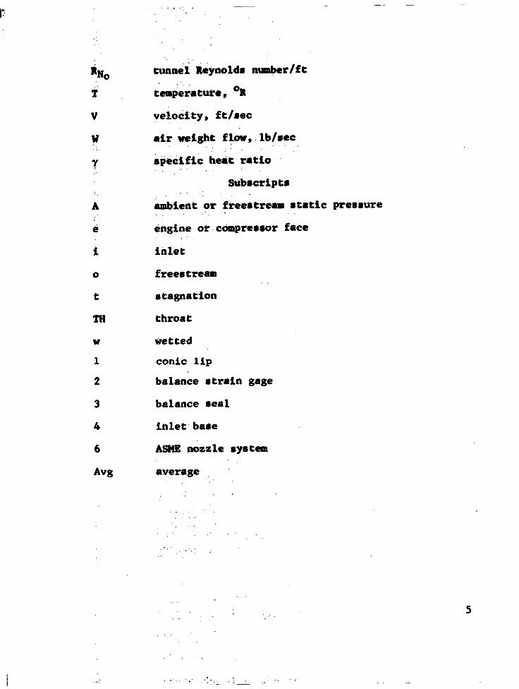
: Rb tunnbi tiaynoldm mm@er/ft

+ temierituite, OR

V

w . .

y

A

e

i

yelocity, ft/rec

air weight flow, lb/ret . ip&A.fic heit ratio .

Subscripts I embient or freertream rtatic prearure . . .-, . kirgine or.cdmprersor face

inlet

0 freertream

t stagnation

TR throat

W wetted

1 conic lip

2 balance strain gage

3 balance seal

4 ihlet'base

6 ASMR nozzle syrtem

Aw average

.

TEST EQUIPMENT AND EXPERIMENTAL METHODS

Facility Description

The test program was conducted in the NASA/Ames Research Center's 6- by 6-foot Supersonic Wind Tunnel. This is a closed-circuit single-return tunnel. It has an asymmetric slid-ing-block:n?~~~~,_an:! a,.test section with perforated floor and ceiling to permit transonic testing. An eight-stage axial-flow compressor driven by two electric motors provides Mach numbers from 0.55 to 2.2. Details of the tunnel test section are shown in Figure 1.

For these tests, the inlet model was attached to the FluiDyne force balance (a flow-metering and force-measuring unit), which was supported by the tunnel sting body and its support system. The metric break on the model was at model station 28.5. A photograph of the installation is presented in Figure 2.

A lo-inch-I.D. pipe carried the air from the flow- metering unit along the tunnel floor for about 38 feet, then through the tunnel floor to the facility vacuum manifold (Figure 3).

Model Description

The model is a l/8-scale simulation of a three-ramp, two-dimensional, variable throat external-compression super- sonic inlet having a design Mach number of 2.2. Model variations consisted of changing the inlet ramp angles and throat area. The variations tested are shown in Figure 4. The model external contour was the same for each configura- tion. The internal and external shape of the inlet is shown by the cross-sections in Figure 5. The internal-duct-flow area distributions are given in Figure 6, and the nacelle normal area distribut'on in Figure 7. the nacelle is 588 in 2

The wetted area for . Cowl and sideplate leading-edge

geometry is presented in Figure 8. All dimensional data are for model scale.

An assembly drawing of the model and force balance is presented in Figure 9; a tunnel installation drawing is presented in Figure 10. Configuration changes were accom- plished by removing one ramp section and replacing it with

6

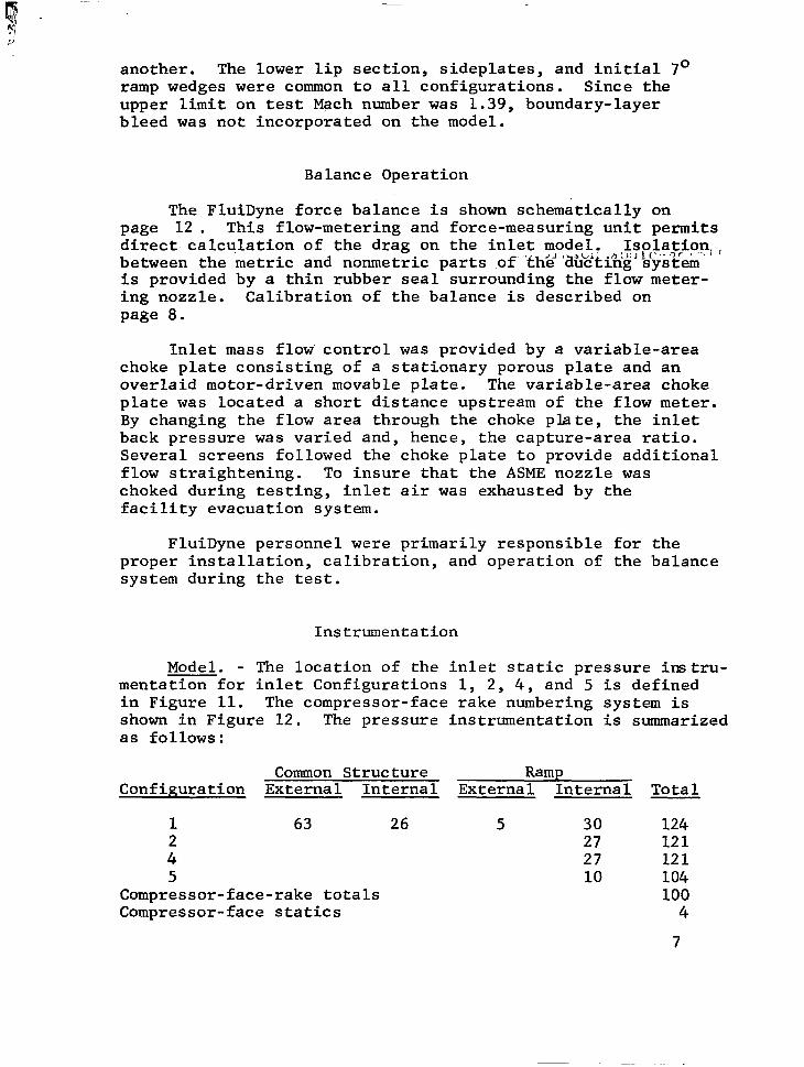
another. The lower lip section, sideplates, and initial 7' ramp wedges were common to all configurations. Since the upper limit on test Mach number was 1.39, boundary-layer bleed was not incorporated on the model.

Balance Operation

The FluiDyne force balance is shown schematically on page 12. This flow-metering and force-measuring unit permits direct calculation of the drag on the inlet model. Isolation;, between the metric and nonmetric parts ,of Uth'eJ'd%ti~g'Ls'$&em‘ is provided by a thin rubber seal surrounding the flow meter- ing nozzle. Calibration of the balance is described on page 8.

Inlet mass flow' control was provided by a variable-area choke plate consisting of a stationary porous plate and an overlaid motor-driven movable plate. The variable-area choke plate was located a short distance upstream of the flow meter. By changing the flow area through the choke plate, the inlet back pressure was varied and, hence, the capture-area ratio. Several screens followed the choke plate to provide additional flow straightening. To insure that the ASME nozzle was choked during testing, inlet air was exhausted by the facility evacuation system.

FluiDyne personnel were primarily responsible for the proper installation, calibration, and operation of the balance system during the test.

Instrumentation

Model. - The location of the inlet static pressure instru- mentation for inlet Configurations 1, 2, 4, and 5 is defined in Figure 11. The compressor-face rake numbering system is shown in Figure 12. The pressure as follows:

Common Structure Ramp Configuration External Internal External Internal

1 63 26 2 4 5

Compressor-face-rake totals Compressor-face statics

instrumentation is summarized

5 30 27 27 10

Total

124 121 121 104 100

4

7

All inlet and compressor-face pressures were measured on the facility scanivalve system. Cycle time was set at 70 sec..

Pressure tubes were approximately 8 feet long. Tubes which originated .at the model as 0.036-in. O.D. were spliced to 0.065-in.-O.D. ,tubing to reduce lag time, but most were 0.065-in-O.D. for their complete length. A lag-time check was made at the beginning of the test to establish the required pressure stabilization time.

Balance. - The balance instrumentation consisted of one strain-gage bridge for the axial load, a digital voltmeter with a sensitivity of approximately 70 counts per pound of applied load for the balance output, and a mercury manometer for balance pressures - with the exception of P7, which was referenced to a tunnel wall static pressure tap through a water-filled U tube.

The balance was calibrated before each run by applying a series of loads in 50-pound increments. Weights were applied axially up to 200 pounds, then removed in 50-pound increments. This process was repeated three times for each calibration. Data from the last two cycles were used to establish the gage factor.

ASME nozzle. - An ASME long-radius nozzle is an integral part of the flow-metering and force-measuring unit. Mass flow data from the nozzle were used to compute capture-area ratio. To insure that the nozzle was choked during the test, the inlet air was exhausted through a system of piping to the facility evacuation system.

Test Conditions

Range of operating conditions. - Test Mach numbers were, 7 0.55, 0.70, 0.85, 0.88, 1.20, and 1.39. At each Mach number the choke plate was adjusted to provide from two to seven values of Ao/Ai. All data were obtained with the model at zero degrees angle of attack

6 The nominal test Reynolds

number per foot was 2.5 x 10 . On configuration 2, at Mach numbers 0.70 and 1.39, data were also

8 btained at Re nolds

numbers per foot of nominally 1.5 x 10 and 3.5 x 10 g . A summary of the test as

Test procedure. - was adjusted to obtain

run is given in Table I.

8

At each Mach number, the choke plate the desired mass flow through the

inlet; data were then recorded. The choke plate was then remotely adjusted for other mass flow rates, as desired. The time between data points was in excess of three minutes.

Tunnel pressures were recorded on digital readout mercury manometers. All inlet pressures were measured by the facility scanivalve system. Balance force data were recorded by an automatic printout device from the digital voltmeter. Balance pressures were recorded by photographing the manometer board.

Computations

Compressor-face conditions. - The average-total pressure recovery, Pte/Pto, distortion (Ptemax-Pt emin) /Pt,, and Mach number, Me, at the simulated engine compressor face were computed from the static and total pressure instrumentation shown in Figure 12. If a tube was plugged or broken off, it was deleted from all listings and computations.

The average Mach number, Me, at the compressor face is computed as follows:

m

Me =

where Fe is the average of four static pressures at the compressor face.

Inlet external skin-friction drag coefficient. - The inlet external skin-friction drag, which is a part of the measured balance force, is computed in coefficient form as follows'i

friction drag cF= qA

oi where

friction drag = Cf q. +J

and where

A w = 588 sq.in. for Configurations 1, 2, 4, and 5

9

_. ..-~ . ..- .---- ..-- -. ..~. --- --- _.. ___ ..-- --_^-

_- 1.1:

-; -- , -,.::- .._’ . .’ i -. . . ~- < >L. _ _ -‘-LA; .. I..__ -. ._--v-. __--_--_._ -- -

- -~ --_ . .

. ‘~ . . . . ,

Cf = 'Cfi (1 + 0.1296 ~) -0.648

(includes compress- ible effects

: . (Ref. 2)) .

*. . Cfi 5 0.455 (the Prandtl-Schlichting @glO %i)2*58 flow) equation for incompressible'

. wi = inlet Reynolds no. - RN0 x 1.94

RNo --' tunnel Reynolds no./ft

1.94 = model average length in ft (Configs.l,2,4,5)

Inlet capture ratio. - Capture-area ratio, defined as the ratio of the cross-sectional area of the captured free- stream tube area, A,, to the inlet geometric reference area, Ai, is calculated as follows:

Ao/Ai *.

['

Inlet Mass Flow Mass Flow per Unit Area at

Freestream Conditions . where

wi=w,

Inlet Mass Flow, Wi = (P/Ptm)6Cd6 A&j

where 1 I s.

and Cd6;'the'discharge coefficient of the choked, standard, long-radius AS.?lE nozzle used to meter the inlet flow, is a function .of flow-meter Reynolds number,

-0.2 cd6 = l-0.184 &J6)

and Mg = 1.0

-- --.

II-. --I__ - -._

For air, Y= 1.4

R= 1716.322 ft2/sec2-OF. ,

Therefore

and

(p/p@) 6 = 0.53177 ,'. '.' .

Wi = 0.53177 cd6 A6 ptfj

JF

W,/A, = g@ 'A/* M, [1 + y MO2 1 1'2

= 0.9189 PA/f0 M, 2 a : I. l/2

D

Finally,

A,/Ai = cd A6Pt6 Go

0.53177 6 0.9189 MO dm PA 66

Inlet drag coefficient. - Total inlet drag, D, is defined as the sum of the axial forces (pressure and friction) acting on the external cowl surface between Stations 0 and 28.5 plus the pressure force acting on the unbounded captured stream- tube between the freestream reference station and the cowl lip. The pressure force acting on the unbounded captured streamtube is commonly known as additive drag. The forces are shown by the following sketch.

11

..--- ---.- -~~_ - __---_ .---- . ..- _- -

.

Free- stream

Sta. 4 Metric ' break sta 28.5

Captured I'; streamtube:

?I Sta. ‘Dadd

cowi Sta.

D cowl lip --i

I -- --

Total inlet drag is then defined as

1 D = Dadd + Dcowl =

J (P-PA)dA + j4(P-PA)dA + Df

0 1

4 4 ‘D=

/ PdA -

l- PAdA + Df

0 0

> -

(1)

A schematic of the model and balance arrangement is shown below.

I A6 r'3 rF6

\ \ / I

i _- I

t . .

'A A4 Tt6 't6 ‘Hz

The summation of the forces gives the equation

s 4

Fo + PdA + Df = Hz + P4(A4-A3') + P3(A3'-A6) + F6 (2) 0

where

F. = y Mo2 PAAo + PAA~

12

--.,------ --. -- -~- _.-- -

1 _ :,; __,_ -~-

. -::

_ - -_ - .‘T-- --.-----y- --- _..

._.. - .~’ \. .:y..’ C., \- 2 ,. ,,

I--

and F6 is the thrust of the choked ASME metering nozzle (Station 6), and A)3 is the effective area of the rubber seal isolating the metric and nonmetric parts. In equation form, Fg is

F6 = P6A6 + m6 v6 = P&j (1 + y Cd6 CT6)

= 0.52828 P,6 4j (1 + y Cd6 CT6)

The discharge and thrust coefficients-'bf the cho k ed ASML nozzle are functions of the nozzle Reynolds number as follows:

Cd6 = ' - 0.184 (RN6) -0.2

-0.2 CT~ = 1 - 0.116 (R&)

Merging Equations (1) and (2) and rearranging,

D = H2 + Pq(Aq-A3') + P3(A3'-A6) +F6 - PO +14 pAdA]

Considering the last two terms in the equation,

Fo + PAdA = YQ' PAAo + PAAo + PA (Ab-Ao)

= Y MO2 PAAo + PAAq

Therefore,

D= H2 + Pq(Aq-A3') + Pg(Ag'-A6) + F6 - Y Mo2PAAo - PA&

or, rearranging,

D - H2 + F6 - P3A6 + (PL+-PA)A4 + (P3-P4)A3' - 1.4 Mo'PAAo

The drag coefficient is obtained fern the drag value by dividing by the product of the freestream dynamic pressure, qo, and the reference inlet area, Ai.

D CD = - 40 Ai

13

Data Accuracy

Error in facility and balance measurements. - The precision of measurements of both the basic-facility-measured and the balance-measured parameters areas follows:

Facility-Measured Pressures and Temperatures _ i

Pto + .Ol "Hg = & .0049 psi : .t

PA + .Ol "Hg = + .0049 psi

PWALL + .Ol "Hg = + .0049 psi

P, + 3/4 of 1% of 12.5 psi = + .094 psi

Tto + 2'F

Balance-Measured Pressures and Forces

P4 = pwALL + P7*

= (2 .0049) + (5 .0025) = + .0055 psi @MS)

p3 = + .017 psi (M:) .1

',6 = + .017 psi (EMS)

H2 + .25 lb (from force calibrations)

On the basis of the facility values and a statistical analysis (EMS) of the possible errors in measurement, 68.3 per-.,,. ., cent of the data for the two ratios P,/Pt, and CP should be within the limits shown below

MO = 0.55 MO = 1.39

px/pt .007 .Oll 0 + 2

CP + .026 + .044

*P7 = (P4 - Pwall) - measured with water filled U tube manometer

14

The relatively 'large potential error in the scanivalve transducer output accounts for most of the above-noted potential error in the ratios.

Error in Ao. - The two primary parameters provided solely by the balance system were A,/Ai, inlet capture-area ratio, and CD, inlet 'drag coefficient. The equation used to calculate A, when the ASME flow nozzle is choked is shown helm. During,the teat;" ' "' \ thenbzzle was choked at all data points but one, which was at a very low Reynolds number.

Ao= 0.53177 A6 cd6 Pt6

. “0 PA

. where m, is a flow function, which for air, is

rho = . 9189 M. dl + .2 Mo2

and it is assumed that Tto = Tt 6 .

The accuracy of the A, calculation can be determined by examining the effects of possible errors in the parameters of the equation. A6, the nozzle throat area, is a constant. Since Cd6 does not change in value in the fourth decimal place even at up to a Z-percent change in RN6, it is eliminated as an error source. Individual errors in Pt6, PA, and MO could cause an error in Ao, as listed below. Thus, most errors in A0 would be quite small.

Percent Error in An

Error MO = 0.55 MO = 1.39

MO 5 ,001 rl: 0.193% + 0.027%

',6 + .017 psi i 0.161% + 0.361%

PA + .0049 psi + 0.046% 2 0.181%

RMS of error % + 0.255% + 0.405%

15

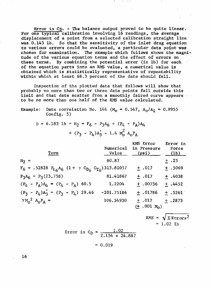
Error in CD. - The balance out,put proved to be quite linear. For one typical calibration involving 16 readings, the average displacement of a point from a selected calibration straight line was 0.143 lb. So that the sensitivity of the inlet drag equation to various errors could be evaluated, a particular data point was chosen for examination. The example which follows shows the magni- tude of the various equation terms and the effect of errors on these terms. By combining the potential error (in lb) for each '- of the equation parts into an EMS value, a numerical value is obtained which is statistically representative of repeatability within which at least 68.3 percent of the data should fall.

Inspection of the plotted data that follows will show that probably no more than two or three data points fall outside this limit and that data scatter from a smoothly faired curve appears to be no more than one half of the RMS value calculated.

Example: Data correlation No. 144 (Mo = 0.547, AoIAi = 0.9955 Config. 5)

D = 6.183 lb = H2 + F6 - P3A6 + (P4 - PA&

+ (P3 - P4)A; - 1.4 Mz AoPA

EMS Error Error in Numerical in Pressure Force

Term Value (psi) 0

H2 = 80.87 + .25

F6 = .52828 Pt6A6 (l+ Y CD6 CT6)313.81057 + .017 + .5069

P3A6 = P3(23.758) 81.41867 + .017 + .4038

(P4 - PA&+ = (P4 - PA) 60.5 1.2204 + .00736 + .4452

(P3 - P4)A; = (P3 - P4) 29.46 -201.75186 + .dlf'8'6 + .5261

YMo2 AoPA = 106.54930 + ,017 + .2873 e .OOl Mo)

RMS = JGkz = 1.02 lb

Error in CD = 1.02 2.154 x 24.887

= 0.019

16

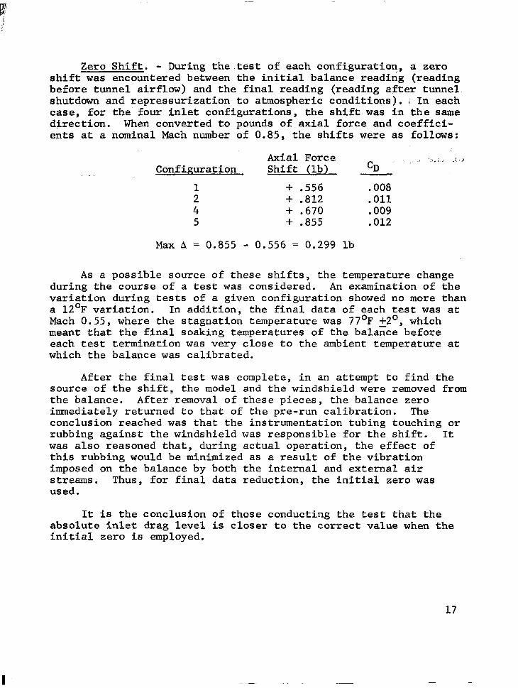
Zero Shift. - During the test of each configuration, a zero shift was encountered between the initial balance reading (reading before tunnel airflow) and the final reading (reading after tunnel. shutdown and repressurization to atmospheric conditions). c In each case, for the four inlet configurations, the shift was in the same direction. When converted to pounds of axial force and coeffici- ents at a nominal Mach number of 0.85, the shifts were as follows:

Configuration

1 2 4 5

Axial Force Shift (lb)

+ .556 + .812 + .670 + .855

cD .i I'. I... .I a

.008

.Oll

.009

.012

Max A = 0.855 - 0.556 = 0.299 lb

As a possible source of these shifts, the temperature change during the course of a test was considered. An examination of the variation during tests of a given configuration showed no more than a 12'F variation. In addition, the final data of each test was at Mach 0.55, where the stagnation temperature was 77'F +Z", which meant that the final soaking temperatures of the balance before each test termination was very close to the ambient temperature at which the balance was calibrated.

After the final test was complete, in an attempt to find the source of the shift, the model and the windshield were removed from the balance. After removal of these pieces, the balance zero immediately returned to that of the pre-run calibration. The conclusion reached was that the instrumentation tubing touching or rubbing against the windshield was responsible for the shift. It was also reasoned that, during actual operation, the effect of this rubbing would be minimized as a result of the vibration imposed on the balance by both the internal and external air streams. Thus, for final data reduction, the initial zero was used.

It is the conclusion of those conducting the test that the absolute inlet drag level is closer to the correct value when the initial zero is employed.

17

.

The plots' in‘Figure 13 for each configuration present the. ik%ment in inlet drag coefficient that should be added to the . . listed data if the final zeros were to be used rather than the',.. ;,, initial zeros. I

If the final rather than the initial zeros had been employed,. the total drag coefficient would be,approximately 0.006 to 0.016 less, depending on Mach number and configuration.

18

EXPERIMENTAL RESULTS

Total Inlet Drag

Total inlet drag coefficient, CD, is presented as a function of inlet capture-area ratio, Ao/Ai, for Mach numbers of 0.55, 0.70, 0.85, 0.88, 1.2, and 1.39 in Figure 14. Inlet configuration (or ramp angle) is presented as a variable at each Mach number.

For each configuration, inlet mass flow was varied, with the upper limit determined by the inlet throat area or, as in the case of Configuration 5, by the balance choke plate maximum flow area. At each Mach number a locus of choke points for each configuration is established and extrapolated to unity capture area ratio. The unity-capture-area-ratio drag levels so determined are plotted as a function of Mach number in Figure 15. Although the extrapolation is somewhat arbitrary, the curve generated is smooth and, therefore, the spillage drag should be of reasonable accuracy.

Generally the data of Figure 14 are well behaved and provide the expected results of decreasing drag with increasing capture- area ratio and decreasing inlet throat area. The exception to the trend of most of the data is at Mach 1.39, where the drag of Configuration 5 is lower than that of Configuration 1. The reason is not obvious but could be associated with the complicated flow field set up by the re-expansion of the flow at the intersection of the first and second ramps on Configuration 5 and the resultant strong terminal shock and possible boundary-layer separation on the ramps.

At Mach numbers of 0.70 and above, and at a given inlet cap- ture-area ratio, a significant inlet drag reduction can be realized by operating the inlet as near the choke point as possible. A tradeoff of course exists between the reduced inlet drag and reduced thrust due to pressure recovery degradation. (The effect of inlet throat area on pressure recovery and distortion is presented in Figure 18 and discussed subsequently).

The estimated cowl skin-friction drag is shown in Figure 16.

The effect of Reynolds number on total inlet drag is shown in Figure 17 for Configuration 2. Reyno ds number variations from approximately 1.5 x lo6 to 3.5 x 10 t!i were made at Mach numbers of 0.70 and 1.39. Inlet drag coefficient is plotted as a function of Reynolds number at captwe-area ratios of 0.45 and 0.62. Increasing Reynolds number decreases the measured drag up

19

to a Reynolds number per foot of about 2.5 x lo6 at Mach 0.70 and 3.5 x lo6 at Mach 1.39.

Pressure Recovery and Distortion

The effects of inlet capture-area ratio and throat area on total pressure recovery and distortion at the simulated engine

,.Fompressor face is shown in Figure 18. The vertical line of capture-area ratio for each configuration corresponds to the capture-area ratio at which the inlet throat becomes choked or

where further reductions in inlet back pressure will not produce any further increase in inlet mass flow.

Lines of constant theoretical throat Mach number, based on geometric throat area and assuming inviscid flow, are superimposed on the plotted data and show a choking Mach number of approxi- mately 0.80 or less for each configuration at each freestream Mach number. A total pressure recovery at the inlet throat of 1.0 was assumed in calculating throat Mach number. It is obvious that, for inlet design and analysis purposes, a throat Mach number of less than 0.80 should be assumed to preclude large losses in total pressure recovery and high distortion.

The low total-pressure recovery for Configuration 5 at Mach 1.39 is due to the re-expansion of the flow at the intersection of the first and second ramps and the high total-pressure losses associated with the resulting strong terminal shock.

Reynolds number effects on pressure recovery and distortion (Mach 0.70 and 1.39) were not significant, based on the limited data obtained.

Ramp and Cowl Static Pressure Distribution

The effects of capture-area ratio, ramp angle, and Mach number on the ramp centerline static pressures are presented in Figures 19, 20, and 21, respectively. The lack of variation of ramp static pressure away from the inlet centerline is shown in Figure 22. Plots of the lower cowl centerline external pressures are presented in Figures 23, 24, and 25. The effect of capture- area ratio is shown for Configuration 1 at Mach 0.85; the effect of ramp angle is shown at nominally 0.60 capture-area ratio and Mach 0.85; and the effect of Mach number is shown for Configura- tion 1 at nominally 0.60 capture-area ratio. The remainder of the pressure data is reported in Reference 1.

20

The effect of decreasing inlet capture-area ratio on the ramp pressures at Mach 0.85 (Figure 19) is to increase the static pressure on the ramps forward to the first-ramp leading edge, with the biggest increase occurring on the third ramp and near the inlet throat. The high negative pressure coefficients near the inlet throat at 0.715 capture-area ratio are indicative of choked flow.

Increasing ramp angle or decreasing throat area at a constant capture-area ratio (Figure 20) has the effect of increasing pres- sure on the first and,second ramp and decreasing pressures on the third ramp. Configuration 2 produces negative pressure coeffi- cients near the inlet throat, again indicative of choked flow.

A large increase in ramp pressure occurs at Mach 1.20 (Figure 21), which partly results in the increase in drag noted earlier. A detached normal shock is produced ahead of the first-ramp leading edge at this Mach number. The shock is attached to the first-ramp leading edge at Mach 1.39, with the terminal-shock pressure rise clearly evident on the second ramp at approximately station 5.0.

In the case of the cowl lower centerline pressures, decreas- ing the capture-area ratio moves the captured streamline stagna- tion point further inside the lip, increases the velocity of the airflow adjacent to the external cowl surface, and results in a decrease in cowl pressure (Figure 23). The increase in pressure coefficient very near the lip leading edge at 0.493 and 0.448 capture-area ratios could be due to the local formation of a separation bubble at these low capture-area ratios.

Decreasing the inlet ramp angle (Figure 24) has the same effect as reducing the inlet capture-area ratio in that the captured-streamline stagnation point moves further inside the cowl lip and results in lower cowl pressure coefficients near the lip leading edge.

The effect of Mach number on cowl pressure distributions (Figure 25) shows high cowl pressure coefficients at Mach 1.2 and low pressure coefficients near the cowl leading edge at Mach 1.39.

21

COMPARISON OF EXPERIMENTAL DATA WITH FINITE-DIFFERENCE FLOW-FIELD SOLUTIONS

The Fort Worth Operation has developed a versatile finite- difference computer code capable of computing the entire flow field about inlets such as those tested in this program. The detailed pressure distributions acquired in the tests offered an excellent basis for an evaluation of the method of analysis upon which the computer code is based. These flow-field solu- tions, used for comparison with the experimental measurements, were computed as a part of the Convair Aerospace Division's IRAD program. Both the method of analysis and the computer code are described in detail in the Appendix; the application to these inlet flow fields is described in the following paragraphs.

The finite-difference solutions obtained and the correspond- ing test conditions are summarized in Table II. Each solution was obtained with a general patch arrangement, as illustrated in Figure 26. Each utilized the method of Godunov, with which the contractor has had the most experience and which has proven by virtue of its combined accuracy and stability to have the best overall perform- ance of all the finite-difference methods incorporated in the computer code (see Appendix). Cell-node coordinates were hand- loaded along each patch boundary, both along the solid surfaces and in the far field. All interior cell-node points were auto- matically generated from these boundary coordinates by a routine built into the program. Because of the high design Mach number (2.2) of the tested inlet, the cowl lip radius is small compared to the inlet height. This necessitates the use of very small cells in the vicinity of the cowl lip. Yet the overall flow field must extend far enough from the inlet to minimize the impact of the far-field boundary conditions on the solution accu- racy. Both of these criteria must be met within a core storage limitation of approximately 2000 total cells on the CDC-6600 computer utilized. Fortunately, the program permits wide varia- tions in cell size, but, even so, the net result is a mesh that is not as fine as desired in any area of the flow field.

The tested inlet is essentially two-dimensional and was analysed as such in the finite-difference program. However, the subsonic duct must make a transition from the 2-D inlet to the circular compressor face. The geometry effects in this area can only be approximated by the 2-D analysis. This was done by main- taining actual contour on the ramp side and by adjusting the inside contour of the cowl to give the same 2-D flow area as does the

22

tpst inlet at corresponding stations. This results in essentially no contour modification in the first 7 inches of the 19 inches of the subsonic duct included in the computational control volume. Since the inlet height is approximately 5 inches, this was felt to be an adequate representation of the subsonic duct portion of the flow field.

Further details of.the finite-difference solutions, including boundary conditions applied, are described below for each of the three cases analyzed.

Case I

Case I was selected before the current test program was started. It was chosen as a typical condition tested during the 1971 research conducted at' FluiDyne Engineering Corporation with the same inlet model. Specifically, the test case chosen was for a freestream Mach number of 0.707, a capture-area ratio of 0.492, and the inlet ramp in Configuration 2.

The complete computational control volume employed 'is illus- trated in Figure 27. (The patch numbering system is as given in Figure 26.) Portions of six patches in the vicinity of the inlet are given in Figure 28. Yet more detail in the region of the cowl lip is given in Figure 29. As can be seen from this figure, the cowl lip is treated as sharp. The computer code is quite capable of handling a body-oriented blunt-lip mesh; however, because of the scale of the lip radius to the overall inlet size and because the use of a blunt-lip mesh would have required more cells in the lip region (to the disadvantage of other portions of the flow field), the sharp-lip approach was chosen. Obviously, pressures predicted in the cells nearest the. lip will be of questionable accuracy.

The Case I finite-difference solution was started from "free- stream" initial conditions (i.e., each flow property in each cell is initialized at the freestream value). Both the "characteristic time" and "cell-skipping" methods (see Appendix) were employed to reduce computation time. A total of 3200 time passes were com- puted before the solution was deemed to have achieved a true steady-state condition. Less iterations would have been needed had not boundary-condition changes been required after the first 1000 iterations. The final boundary conditions employed were:

23

o Upstream boundaries: Density, horizontal velocity, and vertical velocity (actually zero) fixed at freestream values. , pressure by linear extrapolation.

o Top boundaries: Pressure fixed at the freestream value; velocity components and density by zeroth-orderextrapo-

- lation.

o Downstream (external) boundaries: Same conditions as top boundaries.

o Solid boundaries: Pressure determined by Godunov shock- wave-analogy algorithm (see Appendix) as modified to account for surface curvature effects. All fluxes across boundary are zero.

o Subsonic-duct downstream boundary: Horizontal velocity fixed at ideal value determined by inlet capture-area ratio, freestream Mach number, and boundary-to-inlet- area ratio; vertical velocity set to zero; pressure and density obtained by zeroth-order extrapolation.

Computed pressure distributions for the ramp, external cowl, and internal cowl lip are presented in Figures 30, 31, and 32, respectively. Also given on these figures are the experimental data from the test point run at the same condition - nominally Mach 0.7, capture-area ratio of 0.5 (the specific conditions are given in Table II). The computed and measured ramp surface pressure distributions of Figure 30 show good qualitative agree- ment, but, generally, higher pressures were predicted than were measured. This occurs both on the ramps and in the throat region. Agreement between calculations and experiment improves with nacelle station along each straight ramp section. This is not surprising considering the few computational cells, located along each ramp (three on the first ramp and two on the second)'. Additional cells in this vicinity (impossible within the compu- tational environment employed) would almost certainly have improved the agreement in this region. That higher throat pressure coefficient were predicted by the inviscid analysis than were measured is consistent with boundary-layer displacement effects, but better agreement was anticipated.

24

For the predicted and measured pressures along the external cowl surface (Figure 31), again, the finite-difference solution matches the qualitative nature of.the experimental results, giving a negative pressure region just aft of the lip and little pressure variation aft of nacelle station 12. However, the experi- mental data indicate that Cp's approach zero along the aft portion of the nacelle, while the computed solution does not achieve this logical asymptote. Clearly, the computed solution is inadequate along the external cowl and will result in a large error in.the calculated lip suction force.

In the comparison of predicted and measured pressures just inside the cowl lip (Figure 32), considering the approximation of the cowl lip as sharp rather than blunt, the agreement shown in the figure is excellent.

In summary, the agreement between measurements and predictions was quite good with the exception of the external cowl surface. Solution of other flow fields, particularly around airfoils, with the same computer code have shown the solution accuracy tp be a strong function of the number of cells used, particularly in expansion regions. Unfortunately, the mesh employed in Case I fully used the storarage capacity on the CDC 6600; however, a rearrangement of the cells was possible; Such a change was made, and the resulting solution is described as Case Ia below.

A plot of the flow-field streamlines for the Case I final solution is presented in Figure 33. The coordinates for this plot were obtained by integration of the mass flux along column boundaries. These calculations were performed within the computer code, and the resulting coordinates were hand-plotted. That the capture streamline corresponds to 99.2 percent of the input desired capture area is a measure of the error (0.8 percent) between the specified capture-area ratio and the value actually achieved at the final solution. This is quite good considering the rather indirect method in which this condition is imposed on the solution.

The value of a variety of inlet drag items (including addi- tive drag, lower cowl drag, and total inlet drag) were determined or computed from both the experimental data and the computer solution. A comparison of these results is presented in Table III: For each item, the drag is presented interms of a drag coeffi- cient, based on the inlet area and freestream dynamic pressure. The experimental values were computed as follows: ramp drag is by pressure integration along the ramp, using centerline tap data, back to the point on the ramp that an estimated normal to the

25

flow passing through the cowl lip would intersect the ramp surface; addi‘tive drag is ramp drag plus a.momentum difference term from freestream to the estimated inlet face location, based on one- dimensional isentropic relationships; lower cowl drag is by pressure integration, using lower cowl centerline tap data, from the stagnation point to the metric break; the drag designated

'lower cowl + additive" is simply the sum of those two drags; the total drag is from the force balance, with bookkeeping corrections, and does include appropriate friction effects. While the experi- mental total drag includes pressure forces on the entire external surface, the computer model allows a cowl drag contribution from only one surface, that being the external surface of the lower cowl. The computed drags from the finite-difference solution were arrived at as follows: ramp drag is by pressure integration along the ramp to the same inlet-face point used in reducing the experimental data; additive drag is by pressure integration along the actual computed capture streamline; lower cowl drag is by pressure integration along the cowl from the scwl lip to the model metric break location; "lower cowl + additive" drag is again by addition of those terms; skin friction is a computed friction drag for the entire model external surface to the metric break.

As expected from the ramp pressure distribution comparison in Figure 30, the computed ramp drag exceeds the experimental values; numerically, it is about 39 percent higher. The computed momentum difference, having a CD contribution of 0.005 to addi- tive drag, agrees with the difference between ramp and additive drags determined from the computer solution; thus the computer solution additive drag is higher than the experimental value by the difference in ramp drag. As discussed above, very large discrepancies between measured and computed cowl pressures (see Figure 31) exist, and these are reflected in the large difference in lower cowl drag values. A portion of this difference is expected, however, because the two-dimensfonal analysis requires all spillage to occur over this one surface; spillage actually occurs over the other sides of the inlet, with corresponding lip suction effects; the experimental data confirms this effect. The combined lower cowl and additive drag shows the computed value to be low by 20 percent; this is partially due to the spillage effect discussed, but in fact is relatively good agreement and results from the offsetting direction of the errors in additive and cowl drags. The agreement between experimental and analytical total drags is quite good, the computed value being 10 percent higher than the corrected force-balance value. This agreement is, in part, fortuitous but does indicate that the sideplate suction effects are significant and that the two-dimensional analysis

26

‘.

'shows..good potential in the evaluation of-what is in reality'a three-dimensional flow fie-ld about a nominally two-dimensional inlet; No spillage-drag comparison was possible because the u,nity-capture case was not computed-. Having such a solution, would allow more detailed assessment of the analytical technique because the accuracy of computed drag increments could be deter- mined. -

Case Ia

In an attempt to improve the solution along the cowl surface, and yet utilize the Case I solution as a starting condition, patches 3 and 4 were compressed axially in the vicinity of the cowl lip. The overall computational control volume for the revised mesh is shown in Figure 34. The revised mesh in the vicinity of the inlet is shown in Figure 35, and more detail of the revised cell structure near the cowl lip is shown in Figure 36. The modifications are most obvious through a comparison of Figure 36 with Figure 29.

With the Case I solution as an initial condition, an addi- tional 550 time passes were computed. While this did not yield a steady-state condition, it did result in certain improvements in the solution. The ramp pressure distribution for the revised mesh is shown in Figure 37. Comparison of this distribution with that of Figure 30 shows only slight improvement of the pressure distributions on the first two ramps (where the mesh remains unchanged) but shows a significant improvement in the throat region, where the agreement between experiment and computation is now quite good. This effect is felt to be due to the more accurate treatment of the flow field in the cowl-lip region permitted by the revised cell arrangement.

The cowl pressure distribution for the revised mesh is shown in Figure 38. While improvements are evident (see Figure 31), especially in the leading portion of the cowl, the agreement is not yet satisfactory. As stated above, this solution is not yet steady state; examination of the transient trends in the solution shows that all computed data points are continuing to approach the experimental pressure distribution. The changes shown between the Case Ia and Case I cowl pressure distributions are definitely the result of the mesh modifications and are not merely a function of the additional calculations performed. This is illustrated by the data of Figure 39, which shows the transient history at a typical location on the cowl before and after the mesh revisions. While some slight solution dr%ft is still occurring prior to time

27

pass 3200, the marked change in the solution occurs in response to the mesh change. It is estimated that an additional 1.5 hours of computer time might be required for a final steady-state re- sult. However, examination of the solution trends indicates that still-further mesh refinements (i.e., more cells) would be re- quired,to achieve the ultimately desired accuracy.

TLhe cowl lip internal pressure distribution for the revised mesh is shown in Figure 40, and, when contrasted with Figure 32, indicates yet further improvement in this region also.

Case II

The second condition chosen for solution with the finite- difference program is at the same freestream Mach number and with the same ramp configuration but at an increased capture-area ratio, which resulted in choking during the test runs. Three test points were run at the chosen nominal conditions of 0.7 Mach number and 0.62 capture-area ratio. These test points, listed in Table II, differed only in tunnel Reynolds number. The nominal (inter- mediate) test Reynolds number case has been chosen as a basis for evaluation of the finite-difference solution. However, excluding the cowl-lip region, the effect of Reynolds number on the pressure distributions is small; therefore, selected experimental data points for the higher and lower Reynolds number cases have been included in the comparisons to show the effect in the cowl lip region.

The revised mesh used for case Ia was used for Case II with- out modification, and the results of the Ia solution were used as an initial condition. Steady state was achieved after 1950 time passes. Comparisons between computed and experimental pressure distributions along the ramp surface, external cowl, and internal cowl are presented in Figures 41, 42, and 43, respectively.

The computed and measured ramp surface pressure distributions of Figure 41 show generally good qualitative agreement. The characteristics of the computed solution along the straight ramp sections is very similar to that of solutions I and Ia, and the same explanation given for the solution I results applies.

As stated, this case was chosen because the mass flow was near that at which the inlet choked. This is best seen by refer- ence to Figure 18(b), which shows large reductions in pressure recovery in going from 0.59 to 0.62 capture-area ratio, and large variations in pressure recovery at the 0.62 value with changes in

28

tunnel Reynolds number. Thus the comparison of pressure distribu- tion near the throat is of great interest. As seen in Figure 41, the computed solution did not yield as low Cp values in the throat as were measured. This is as expected, however, since at these near-sonic conditions the flow is very sensitive to the boundary- layer displacement effects, and the smaller effective flow area results in lower measured Cp values. In both the test run and the computed solution, supersonic flow is indicated by the throat C 's; a weak normal shock at nacelle station 10.0 is predicted-in, t E e computer solution but not evidenced, at least upstream o.f .station 10.4, in the test data.

A comparison of computed and measured cowl external pressures is given in Figure 42. Good qualitative agreement is seen but, as in Case I, the predicted Cp 's are generally lower than those measured. This is especially true near nacelle station 10.0 and would result in an optimistic lip suction force prediction. A closer inspection of the cowl contour used in the finite-difference solution shows a very slight irregularity in the specified co- ordinates in this region; as expected, the inviscid solution is much more sensitive to such details than is the actual viscous flow. Better specification of the contour and more cells along the cowl would have yielded an improved solution, but machine storage capacity limitations prevented this.

The pressure distributions inside the cowl lip (Figure 43) do not agree as well as in the Case I solution. As stated previously, this is a very small region close to the lip, and the sharp lip assumed in the computed solution does limit accuracy in this region. It should be noted, however, that the change from large positive Cp 's in this region in Case I (Ao/Ai = 0.50) to negative Cp's in Case II (Ao/Ai = 0.62) is predicted by the finite- difference solution.

29

CONCLUDING REMARKS

Accurate inlet spillage-drag data were obtained on a realistic two-dimensional, variable-geometry, external-compression, supersonic inlet configuration over a wide range of inlet compression-surface angles, mass flows, and subsonic and transonic flight speeds.

High inlet-capture-area ratios were obtained, enabling a credible extrapolation of the measured inlet drag to a capture- area ratio of 1.0.

Generally, the experimental data were consistent and provided the expected trend of decreasing spillage drag with increasing capture-area ratio and decreasing inlet throat area.

Large losses in inlet total-pressure recovery and increases in compressor-face distortion were observed at high inlet-throat Mach numbers. The choking inlet-throat Mach number observed, based on geometric throat area, was 0.80 or less. These data provide a basis for determining the tradeoff between inlet spillage drag and pressure recovery for practical design applica- tions.

The computed flow-field solutions agreed reasonably well with the measured pressure distributions for the corresponding inlet flow conditions. It was established that finer meshes will result in yet more accurate solutions, but the desired refinements will require a computer having more core storage capacity than the CDC-6600 employed. The analytical technique shows good promise for the evaluation of inlet drag through use of a two-dimensional model, but further drag prediction comparisons are needed.

Since the computer code can handle subsonic, supersonic, and mixed flows, the subsonic solutions reported do not represent a complete utilization and checkout of its capabilities. Further evaluation of the full potential of thz code should be made, preferably in a larger, faster-computing environment such as the CDC-7600 or, even more ideally, the NASA Ames Iliac 4. Other test cases from this experimental study provide an excellent basis for such an evaluation.

30

APPENDIX

DESCRIPTION OF THE FINITE-DIFFERENCE METHOD OF ANALYSIS AND THE COMPUTER PROGRAM

The computer procedure employed to provide the analytical solutions utilized in this study was formulated to solve numeri- cally (using explicit finite-difference techniques) the equa- tions, describing the transient, two-dimensional or axisymmetric flow of an inviscid, compressible, perfect gas. The rationale employed in the development of the computer procedure was to provide a computational framework that could be used to treat a wide variety of problem types. To this end, a number of op- tions are included, permitting, for example, selection of the particular differencing scheme to be used, control of the calcu- lation process, and specification of the type and volume of out- put data. The versatility of the program is derived from (1) the availability of several finite-difference schemes, (2) the flexibility of the flow-field mesh arrangement, and (3) the variety of boundary conditions available.

Thus, while the finite-difference method of Godunov (Refer- ence 3) was employed with this procedure to calculate inlet nacelle flow fields for the current effort, it has also been used with this procedure to calculate airfoil flow fields. Also, with this same computer procedure, other finite-difference methods (i.e., the MacCormack, Brailovskaya, and donor-cell methods - References 4, 5, and 6, respectively) have been used to calculate simpler flow fields. In addition, a closely re- lated computer 'code with,more limited geometric capabilities but with the viscous and heat-conduction terms of the Navier-Stokes equations has been used successfully to calculate subsonic, supersonic, and hypersonic attached boundary-layer flows (both laminar and turbulent) and to calculate laminar separated flows. The descriptions which follow are oriented toward the aspects of the analysis employed to generate the solutions utilized in this study.

Method of Analysis

The basic approach is to solve, using finite-difference techniques explicit in time, the. equations that describe the transient flow of a compressible, inviscid, perfect gas. The desired steady-state flow field is a result of the solution

31

progressing asymptotically from an initial condition to the steady-state condition. The basic equations are applied as follows:

1.

2.

3.

4.

The flow field is divided into a finite number of discrete cells, with flufd properties assumed constant within each cell.

The governing equations are applied in integral -form to each cell as a control volume to describe the time rate of change of mass, momentum, and energy within the cell in terms of the transport of these properties (fluxes) across the cell boundaries.

The fluid properties at the boundaries between cells are used to evaluate the fluxes. These properties are calculated by any one of several simple algorithms, which are described in de- tail below.

Appropriate boundary conditions are applied at the extremities of the overall flow-field con- trol volume. .

Governing equations. - Use is made of the continuity, mo- mentum, and energy equations in integral form. These equations, in non-dimensionalized form, are as follows:

Continuity:

a

at s pdv =

C.V. (control - volume) surface)

Momentum:

a s ,ij-.& = -. .F C.V. S r (pi74i) - p&J '

C.S. C.S.

32

(2)

Energy: I 7

a s

pEdv = - at: c .v-.

,s (E + p/p) p%%

C’. s . (3)

where E = (+iM + T2 and Y is the. ratio of specific heats. p, 7, E, p, and t represent density, velocity, total energy, pressure, and ,time, ,respectively.

The quantities in these equations are dimensionless. The following list presents the reference quantities used to make them dimensionless.

Dimensional quantity 1

Length .

Velocity

Time

Density

Pressure .‘ .~.

Energy

Reference quantity

L, reference length

U, freestream velocity

U/L

PO, freestream density

PoU2

U2

Formulation of Finite-Difference Equations. - Application of the continuity, momentum, and energy equations to an indi- vidual cell results in the basic finite-difference equations used in the analysis. these take the form

For one-step techniques such as Godunov, '.. . .

( + At = Bit + F . Fi (4)

where V is the cell volume and At is the computational time step. For two-dimensional-.flow, @i and Fi take the form shown below, where u and v are the horizontal and vertical components of 'i and TX and zy are unit vectors in the horizontal and verti- cal directions.

33

The entire flow field consists of cells which are arbitrary quadrilaterals; however, to illustrate the application of these equations, the expressions for Fi have been expanded for a simpler, parallelogram-shaped cell as follows:

where u' and v' represent horizontal and normal velocity com- ponents at the inclined boundaries. The resulting form of the Fi are shown below.

34

- -- ----------r-- - ‘. ‘:

. : , ,. ,. . . . . - ... -- 1;’ ._ . ----- -- *..- . . . . . . ;- .:-’ :. .

; : ‘.. a..

, .,L;:~yy’.).‘. *;,. L , .,’ ., , ,;,,7---- ’ 2 . .

.a:. .

Calculation of Fluid Properties at Cell Boundaries. - Equa- tion 6 describes the fluid properties in the cells (it is applied once per cell per time step) at time t + At in terms of the properties in the cells at time t and the transport of these propert+es across the cell boundaries. A number of methods for evaluating the cell boundary properties are proposed in the literature. Four of these techniques (References 3 through 6) that are compatible with the basic program structure (applying the conservation equations to arbitrary cells) have been incorpo- rated into the computer program. The Godunov scheme has ex- hibited the best overall behavior, especially in terms of numeri- cal stability, and consequently has been employed to generate the solutions in this study.

35

. . . ‘_

BasicaUy, the Godunov method evaluates the fluid proper- ties (velocity normal to cell boundary, p, and p) at a cell boundary- by,considering the adjacent cells and their common boundary to be analogous to the one-dimensional shock-tube prob- lem as shoti in the following sketch.

The location of the diaphragm of the shock tube represents the cell boundary. The properties on either side of the dia- phragm are given by the components of the properties in the re- spective cells at time t. If the diaphragm is suddenly removed, a wave pattern is established in the tube that comprises a compression wave, an expansion wave, and a contact surface, as illustrated below.

The solution of the one-dimensional equations of fluid motion yields the fluid properties in each of the four regions. The fluid properties at the cell boundary are then defined by recognizing the region of flow that exists at the cell boundary.

Flow-Field Boundary Conditions. - Since the conservation equations governing compressible, time-dependent flows are parabolic, they require specified values for p, p, u, and v, or their derivatives, at every cell boundary on the flow-field control-volume boundary. Because steady-state solutions are being sought, steady-state boundary conditions are required. Proper specification of boundary conditions is essential if a physically valid solution is to be obtained; improperly speci- fied boundary conditions can produce incompatibilities that may cause disturbances to propagate throughout the flow field and

36

Region 1 Region 4

////////////~/f///f/////////////////// Diaphragm

Pl

\\\\\\\\\\\\\\\\\\\\\\\\\\\h\\\\~.\\\\\\ I '4 I

Wave Cell Boundary Location Surface Wave

even destroy the stability of the solution. Therefore, special attention must be given to the boundary conditions, and the optimum set of boundary conditions will vary from problem to problem and from one finite-difference technique to another.

Basically, three types of boundaries must be considered:

1. Inflow boundaries

2. Solid boundaries

3. Permeable boundaries.

Boundary conditions for each type of boundary are implemented in the computer programs by the equivalent of surrounding the flowifield control volume by a perimeter of imaginary (or "image") cells, and defining the required properties at the ' centers of these cells.

37

Specification of inflow boundary conditions for supersonic flows is straightforward. Since disturbances do not propagate upstream in a supersonic flow, the inflow boundary is not in- fluenced by the downstream flow. The freestream properties are thus the values to be specified. For subsonic flows, however, disturbances from downstream can propagate upstream and influence conditions at the inflow boundary. It is therefore inappropriate to specify all of the flow properties at a subsonic inflow bound- ary. The technique employed is to set the velocity at the in- flow boundary equal to the freestream velocity. The pressure is then determined by first-order extrapolation from the interior flow field. The density at the inflow boundary is then computed by requiring that the total enthalpy at the inflow boundary be equal to the freestream total enthalpy. In order to minimize the effects of errors introduced by this boundary condition, the inflow boundary is placed as far from the body as is feasible within the restraints imposed by the mesh size.

For a solid boundary, the only appropriate boundary condi- tion is that the normal component of velocity be zero. Wall pressure is, however, specifically required by the computational process, and the calculation of wall pressure has proven to be very critical; different methods have been successful with par- ticular finite-difference techniques. For the Godunov method, the shock-wave-analogy algorithm used between interior cells is applied. This calculation has been generalized to incorporate surface-curvature effects as suggested in Reference 7.

The correct values for the flow properties at the permeable boundaries (i.e., the downstream and lateral boundaries) are generally not known in advance. For supersonic outflow, the solution is insensitive to outflow boundary conditions as long as they do not introduce instabilities. For subsonic outflow, however, conditions must be imposed which, in some sense, least disturb the interior (upstream) flow. The approach taken is to compute properties at the permeable (outflow) boundaries by extrapolation from the interior flow field. As for inflow boundaries, the permeable boundaries are located sufficiently far from the body to minimize the effects of errors introduced by the selected boundary conditions. A specific exception is the subsonic duct downstream boundary in an inlet flow field. Here it is impossible to move the boundary to minimize the effects on the solution. In fact, sufficient conditions must be imposed to achieve the desired capture-area ratio. In sub- sonic flows (or supersonic flows that can be considered as isentropic), the boundary condition used with the most success

38

is one in which the axial velocity is fixed at the ideal value based on isentropic flow (assumed uniform at the outflow bound- ary) and the pressure and density are extrapolated (zeroth order). The velocity component parallel to the outflow boundary is set to zero. For supersonic flows (where a loss of total pressure is expected) the capture-area ratio, continuity equar tion, and total energy equation can be combined to yield the ideal values of pressure, density, and axial velocity which should exist if the flow were uniform at the outflow boundary. ' These values, along with a zero velocity parallel to the boundary, are imposed as the boundary conditions at each cell on the out- flow boundary.

Flow-Field Initial Conditions. - Inasmuch as the asymptotic steady-state solution depends only on the boundary conditions imposed, the specification of initial conditions should affect only the time required to obtain a solution. (However, if ini- tial conditions are exceptionally inconsistent with the boundary conditions, startup problems may result and preclude a steady- state solution.) Successful use has been made of impulsive initial conditions (i.e., starting from freestream conditions), input "best guess" initial conditions (based on intuition or prior knowledge), or the final solutions of previously calcu- lated flow fields as initial conditions.

Computer Program Description

The computer program which implements the method of analysis described above is designated as General Dynamics' Convair Aero- space Division Procedure TP4. So that core storage requirements are reduced, the computer procedure is logically divided into three separate programs, designated TP4-I, TP4-II, and TP4-III. The TP4-I program performs flow-field-mesh generation and initial- condition setup; TP4-II performs the actual flow-field calcula- tions; TP4-III performs additional computations (such as stream- line locations) on the flow-field data when a final solution is achieved. Unless otherwise stated, the information which follows refers to the overall capabilities of the three separate TP4 programs.

The versatility and flexibility of the program are derived primarily from (1) the flexible mesh-patch structure, (2) user control of boundary conditions through input data, (3) compre- hensive output data, and (4) special features that enhance the

39

efficiency and increase the utility of the program. These features combine to yield a program that is definitely "user- oriented." Control of the finite-difference technique employed is ,als'o available through input data, but because the solutions reported hereTare derived with the Godunov method, this aspect of,-the--program will be discussed in no further detail. Also; the--flow fie.1d.i.s specified as either rectangular or axisymnetric by a single input option code.

: The mesh-patch structure, boundary-condition options,.

special features, and input/output are discussed in the follow- ing paragraphs.

The Mesh-Patch Arrangement. - The development of a procedure for treating a wide variety of flow geometries requires a versa- tile mesh-geometry arrangement to treat complex body shapes. This capability is provided through the use of a mesh-patch arrangement. With this arrangement, complex mesh geometries are built up from simpler sub-meshes or "patches." The following simple example illustrates the use of the mesh-patch arrangement;

Consider the flow through a two-dimensional channel having a step as illustrated in Figure 44(a). A mesh arrangement con- sisting of-three patches is shown in Figure 44(b). Each patch consists of a logically (but not necessarily geometrically) rectangular array of cells, i.e., each patch consists of M columns and N rows of quadrilateral cells. (M and N may be different for each patch except for certain restrictions on ad- joining patches.) Thus, each patch has four boundaries, as illustrated.in Figure 44(c).

The program allows for meshes comprising up to 20 patches. With this capability, mesh geometries can be constructed for quite complex flow fields. Sample mesh-patch arrangements for some types of problems are illustrated schematically in Figure 45.

One of the attractive features of the finite-difference scheme employed- is the use of a non-orthogonal body-oriented mesh geometry. This feature facilitates the application of boundary conditions along arbitrary surfaces; however, it also presents the user with the frequently arduous task of defining the non-uniform mesh geometry. The mesh geometry is defined by specification of the coordinates of the corner points (or 'nodes") of the quadrilateral cells. For a general non-orthogonal, non- uniform mesh, this often involves the specification of coordi- nates for several thousand points. The probability for errors

in generating, transcribing, and keypunching such a large number of coordinates is quite high.

One way to reduce the probability for errors is to reduce the amount of input geometry data required. This can be accom-, plished by generating the coordinates of all the interior nodes of a mesh patch with the program. This technique requires only the coordinates of node points on the four patch boundaries. - Briefly, the interior node coordinates are generated for an arbitrary four-sided region (in a plane) from a set of known points along each of the four boundaries. The known boundary points are first mapped onto the corresponding boundaries.0f.a unit square. Straight-line connection of these boundary points is then used to define interior&node points in the unit square. The interior points within the unit square are then transformed back to the physical plane by use of a technique based on a surface-definition method of Coons (Reference 8).

With this geometry-generation method, only the points on the patch boundaries are required. For curved surfaces, these point 'coordinates must be furnished. For patch boundaries that are straight lines, however, an additional simplification of the input has been accomplished by a technique for subdividing a straight line into a monotonically increasing (or decreasing) set of intervals. Through this technique only a few input parame- ters are necessary to generate the point-coordinate data for a straight patch boundary.

A sample application of the mesh-geometry generation scheme is presented in Figure 46. The four boundaries of this sample mesh patch are defined as follows:

Boundary 1: The straight line from (-0.25, 0) to (-0.75, 0)

Boundary 2: The straight line from (0, 0.5) to (0, 1.2)

Boundary 3: The second quadrant of the ellipse

Boundary. 4: The second quadrant of the ellipse

.', 41

The coordinates for the points along Boundaries 3 and 4 were generated from the above relations and input directly. The points along Boundaries 1 and 2 were generated by use‘of ,' '. the technique developed for straight patch boundaries. The co- ordinates of the interior points were generated by the mesh- geometry generation scheme.

The geometry plot in Figure46 was generated by an SC-4020 computer recorder. Such computer-generated plots provide a rapid- and -graphic means of assessing the suitability of the computer-generated mesh geometry as well as of detecting geometry input errors.

The Boundary-Condition Options. - The mesh-patch arrange- -- ment described above requires the specification of boundary con- ditions for each patch boundary. So that maximum flexibility would be provided, the program was coded to permit the selection of any of several available boundary conditions for each of the. four boundaries of each patch. In addition, it was necessary to provide for the calculation of the cell boundary fluxes on those boundaries common to two adjoining patches.

The calculation of the properties on a common boundary is accomplished on a cell-to-cell basis within the computer pro- gram. That is, each segment of the common patch boundary is shared by two (and only two) cells. Thus the two patches ad- jacent to the common boundary must have the same number of cells along that boundary, and the cell spacing along that boundary must be the same for each patch. Once the cells involved are identified, the cell boundary fluxes are computed by use of the same scheme used for interior cell boundaries.

The boundary condition applied at any patch boundary not shared with another patch can be selected via input option from any of the following types: For inflow boundaries, options for subsonic or supersonic inflow are available. For outflow boundaries, extrapolation techniques are generally employed, and both zeroth-and first-order (linear) extrapolation options are available. A special boundary condition is provided for inlet flow fields for use at the subsonic duct outflow boundary so that the inlet captures the desired mass flow. For solid surfaces, the pressure on the boundary may be determined by extrapolation from the flow field adjacent to the surface or may be computed by use of the Godunov scheme to determine the pressure required to cancel the normal component of momentum in the adjacent cell. For the latter case, surface curvature effects

42

may also be included. In addition, boundary-condition options for the axis of symmetry for axisymmetric flows and other special conditions are also.available. i i

The optimum boundary-condition options may vary from prob- lem 'to problem and from one finite-difference scheme to another. The program allows the user to select the boundary condition most appropriate for a given problem from an array of boundary-. condition options. In addition, the program has been so coded. that additional boundary-condition options may be incorporated .in a 'straightforward manner.

Special Features. -. Several special features have been in- cluded in the inviscid flow-field program to enhance its ef- ficiency, and increase its utility.

All of the data required to restart the solution may be written on magnetic tape at selected intervals during a com- puter run. This capability allows lengthy problems to be run as a series of lower-risk computer runs and, also, ensures that an entire run will not be lost because of an abnormal termina- tion (e.g., exceeding the run-time estimate). This feature also permits the user to analyze intermediate results and identi- fy potential problems before proceeding with the solution. When restarting with data from a previously generated magnetic tape, the user may alter any of the options controlling the computa- tions (e.g., boundary-condition options).

The solution may be obtained as a true time-dependent phe- nomenon by the use of the same time step for each cell in the mesh or as a characteristic-time (non-uniform time step) solu- tion wherein each cell is advanced by a time step based on its own local stability conditions. The latter approach conserves computer time when only a steady-state solution is required, especially when large variations in cell size are present. ,. _'.. ,:., ,I

Another tool to reduce computer time, a "cell-skipping" scheme, is available. Cells in which the properties are changing much less rapidly than in the most active portions of the flow field are intermittently omitted from calculational update. The skipping frequency is controlled by relative fluctuation sizes and by an input limit on the number of successive times an in- dividual cell may be skipped.

If it is desired to begin a solution from a non-uniform initial flow field, the Mach number, local flow angle, total

43

pressure ratio (relative to the freestream value), and total temperature ratio may be input at cdkr&r'cells of"e&h'patch (or sub-patch if further definition.. is .desired) and' the initial conditions at each cell will be computed by interpolation from these points. This feature is-utilize'd to reduce. cox&utation time or to minimize the possibility of severe startup-transients

' causing instabilities.

A streamline-tracing routine for the generation of coordi- nates of points on selected streamlines has been developed for nacelle-type flow fields.

Input/Output. - The flow-field program input and output in- formation is summarized as follows:

Input data:

. Flow-field control volume and mesh arrangement.

. Freestream conditions.

. Options controlling mesh-patch boundary conditions.

. Initial conditions for the flow field.

. Options controlling output, use of special features, convergence criteria, etc.

Output data:

. Fluid pressure, density, velocity components, Mach number, velocity vector direction and magnitude, and total enthalpy for each cell in the mesh at selected intervals.

. Similar data for selected cells for each time pass.

. Fluid pressure, density, velocity components, Mach number, and pressure coefficient for selected patch boundaries, e.g., solid surfaces.

. Printed data for pressure, density, and/or Mach- number contours.

. Printed data for streamline traces.

44

- --- ~~--~ .___ -___ --___

. Computer-generated plots of the mesh geometry and velocity-vector plots.'

. Complete flow-field data on magnetic tape for restart problems.

.

45

-. _ _._. ..-- ___ --.--- ---- ---- -.--- _I_ --_--_--~_~_~- ___.

1.

. 2.

3.

4.

5.

6.

7.

8.

REFERENCES

Turner, R. L.: Wind Tunnel Data Report, l/8-Scale Supersonic Inlet Model Tested in the NASA/Ames 6x6-Foot Supersonic ' Wind Tunnel. Vol. I and II. Rep. FZT-246, General Dyrunics' Convair Aerospace Division, June 1, 1973.

Schemensky, R. T.; Braymen, W. W.; and Crosthwait, E. L.: Aerodynamic Configuration Analysis Procedure, Aeromodule, Version lA. Rep. ERR-FW-931, General Dynamics' Fort Worth Division, Dec. 31, 1969. Y.

Godunov, S. K.; Zabrodyn, A. W.; and Prokopov, G. P.: A Difference Scheme for Two-Dimensional Unsteady Problems of Gas Dynamics and Computation of Flow with a Detached Shock Wave. Cornell Aero Lab. Transl. by I.. 0. Bohechevsky. Translated from Zh. Vychisiliteloni Mat. i. Mat. Fiziki, Vol. 1 (1961), p. 1020.

MacCormack, R. W.; and Paullay, A. J.: Computational Efficiency Achieved by Time Splitting of Finite-Difference' Operators, AIAA Paper No. 72-154, 10th Aerospace Sciences Meeting, San Diego, Calif., Jan. 1972.

Allen, J. S.; and Cheng, S. I.: Numerical Solutions of the Compressible Navier-Stokes Equations for the Laminar Near Wake, Phys. Fluids, vol. 13, no. 1, Jan. 1970. ;

Roache, P. J.: Numerical Solutions of Compressible and Incompressible Laminar Separated Flows. Ph.D Dissertation, Univ. of Notre Dame, Nov. 1967.

Masson, B. S.; Taylor, T. D.; and Foster, R. M.: Applica- tion of Godunov's Method to Blunt-Body Calculaticns. AIAA Journal, vol. 7, April 1969, pp. 694-698.

Coons, S. A.: Surfaces for Computer-Aided Design of Space Figures. Memo 9442-M-139, Electronic Systems Laboratory, Massachusetts Institute of Technology, Cambridge, pass., 1964.

46

,- . ..- -------.y .. - ,_ ‘.. _1 ‘7. 5.. -,,.-- ._- . .

.‘i,,, ., -, y- _ _ - -:*, . - ^ - I

TABLE I. - AS-RUN TEST PROGRAM - ~/~-SCALE INLET DRAG MODEL (A-FMGD) TEST NO. 66-695

Angle of Attack = 0'

Run M. Reynolds No./ft Config. Ao/Ai Schedule No. Code

1 2

z DATA NOT AP?LICABLE 5 I 6 1.40 2.5 x 10 6 1 .77, .74, .68, .63, .58, .53 7 1.20 2.5 1 .72, .68, .62, .57, .53, .48

i 0.85 0.88 2.5 2.5 1 1 .71, .71, .67, .66, .62, .60, .56, .54, .52, .49, .46 .45' 10 0.70 2.5 1 .76, .69, .65, .59, ,54, .50 11 0.55 2.5 1 .87, .84, .79, .75, .70, .59

12 1.40 1.5 2 .63, .46 13 1.40 2.5 2 .62, .58, .53, .49, .45, .44 14 1.40 3.5 2 .43, .61 15 1420 2.5 2 .58, .53, .48, .44, .41 16 0.88 2.5 2 .57, .54, .50, .46, .41 17 0.85 2.5 2 .58, .53, .49, .45, .41 18 0.70 1.5 2 .62, .45 19 0.70 2.5 2 .62, .59, .54, .49, .44 20 0.70 3.5 2 .43, .62 21 0.55 2.5 2 .71, .65, .60, .54, .51

22 -- -- Data Not Valid -- 23 1.40 2.5 4 .49, .47, .45, .42 24 1.20 2.5 4 .46, .43, .40 25 0.88 2.5 4 .46, .43, .40 26 0.85 2.5 4 .46, .45, .42, .40 27 0.70 2.5 4 .50, .46, .43 28 0.55 2.5 4 .57, .55, .53, .51, .5Q

29 1.40 2.5 5 .86, .81, .77, .71, .66, .59, .59 30 1.20 2.5 5 .83, .78, .76, .71, .66, .60 31 0.88 2.5 5 .83, .81, .78, .73, .68, .62 32 0.85 2.5 5 .83, .79, .73, .69, .63, .59 33 0.70 2.5 5 .89, .86, .82, .76, .71, .65 34 0.55 2.5 5 1.02, 1.00, .94, .89, .83, .-76

47

___ _ ._ _ . . __- .-...- -- -~ ._-.. .._.. -.. ._ _____._ -__ _ .- - -_-- _.--.-.-

TABLE II.- SUMMARY OF FINITE-DIFFERENCE COMPARISON CASES L c i. .:'., 5 ',, < * 7 , ,)

: * I , .' :: ;.*t.. . Case

Item I I Ia I II ', :. ; . . (Z .. . 2.. Nominal Conditions rl' .:. *

R&p, configuration‘ 2 2 _ . .' 2

Nominal Mach number 0.7 0.7 *I. .“0;7 ‘ , *

Nominal capture-area ratio 0.50 0;5d ' '0.62,

.Figure (No.) shaking results 30-33. +37-4(j I.. : ..4&43 ,.

Test Conditions :. , ~_' :.,.: _,,

Run numbers 19 19 :18,19*,2O‘i * .

Mkh'number 'I" 0.700 0.700 l' 0:7'0~~,0:701*, 0.699

Capture-area ratio 0.491 0.491 0.621,0.618*,

Reynolds numberlft x low6 0.621

2.64 2.64 1.55,2.64*,3.6;

Computer Solution Conditions

Mach number 0.707 0.707 0.700

Capture-area ratio 0.493 0.493 0.62 _'

Figure (No.) showing mesh 27-29 34-36 34-36

Number of cells 1785 1785 1785

Initial conditions Freestream Case I Case Ia Solution Solution

Number of time passes 3200 550 1950

Computer time, hr 5.0 0.6 2.0

*Conditions selected for comparison in Case II

"48

.A.- . .. -- .:.‘: 1..

. r- :. ,--; ; F.,, ,* . -.a ,,~. - _- ,. ,’ .I

TABLE III. - COMPARISON OF MEASURED AND COMPUTED DRAGS FOR CASE I -

Drag Item Drag Coefficient, CD

Experimental Computed

Rami9 0.150 0.208

Additive 0.155 0.213

Lower Cowl -0.033 -0.115

Lower Cowl + Additive 0.123 0.098

Computed Skin Friction -- 0.088

Total Drag 0.169 0.186

.

-

49

_ -.-- _-__ ._ -- ------- .-

-

50

\. \: \. \ \ \ \: ii

I -

,

51

Figure 3.- Vacuum line from model to tunnel evacuation system.

52 c. _ -

.: -’ -.- i-.. r--- . 1 _-T --r- _ TV---- - - ._

_./, .._ ,:.. I . _...I .:..: I.-, -, : : ‘- - ,. .,

_ . : r ‘.

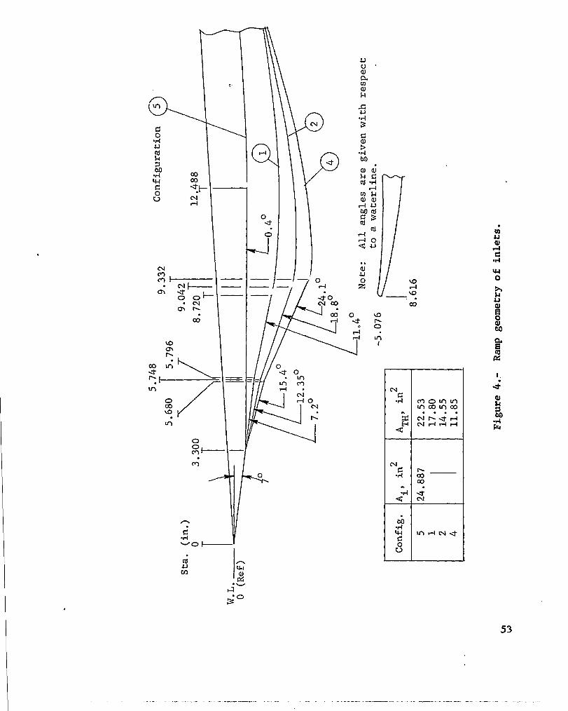
53

..-. ._ -.-_- -.-___..-_- . . .~ -.-_- _._----~ _....._ --..- .-_-- -.- .---- -..- .._. -

,

-- _- -,- --m.,-- . : _. 5 . / . -

. . :.’ * ’ .: *. ,. . .

I 1. !

./ I

i

I 8.818 _____I .

4.,20 i T-II I -

/

i I --------t-- --

1

- 8 I --i-----e--- -

A- - .-- --

\

d . .

-\

: . . ‘.

. ! .,

I 1 -- --

r T&o 1 .I 1

,RONT VICW

GURATION I - I I-/ I

CONClGURAlD,, t

CONFIGURATION .

26

24

22,

20

18

16

14

12

10

Nacelle station, in.

Figure 6.- Model duct flow area distribution.

kt

d l Fl

Nacelle station, in.

Figure 7.- Model nacelle normal area distribution.

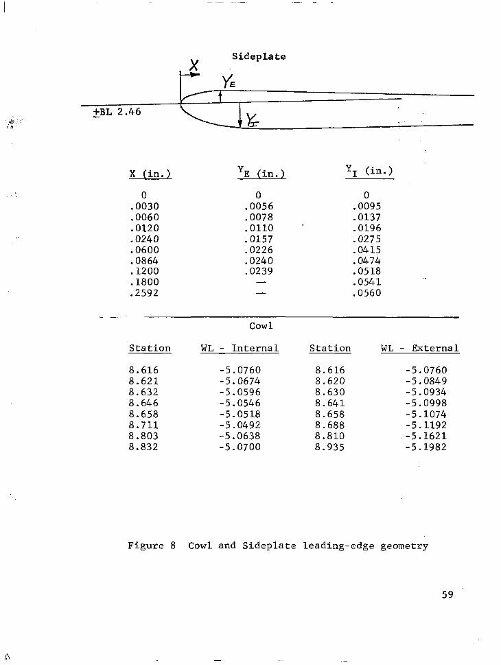
+BL 2.46

x Sideplate

Y E

IY J=

X (in.) (in.) 'E YI (in.)

0 .0030 .0060 .0120 .0240 .0600 .0864

1200 :1800 .2592

0 .0056 .0078 .OllO ' .0157 .0226 .0240 .0239

- -

0 .0095 .0137 .0196 .0275 .0415 .0474 .0518 .0541 .0560

.____.__ Cowl

Station WL - Internal Station WL - External

8.616 -5.0760 8.616 -5.0760 8.621 -5.0674 8.620 -5.0849 8.632 -5.0596 8.630 -5.0934 8.646 -5.0546 8.641 -5.0998 8.658 -5.0518 8.658 -5.1074 8.711 -5.0492 8.688 -5.1192 8.803 -5.0638 8.810 -5.1621 8.832 -5.0700 8.935 -5.1982

Figure 8 Cowl and Sideplate leading-edge geometry

59

Break

Figure Q.- Model and force balance assembly.

:-.

<lUNNEL--

CTUNNE L t

36.0

,-ZDS-251-7 YOKE &HZ)

r 36.0

-. -

36.0

L

I - -

I -

.&M~DEI- ___. I

,&AZ-- ’ --

II I

” ’ --

.I- -.._-_

PARTlhL INSTALLATlON DRAk MODEL AND DALBNCE IN AMES

.-- -. *“.--. L-- ._- ---. -. ---- - ..-

-‘-- .-,.-,- _ ._._ --.:- .. - ..w .._... . ..- -r,--‘- - . . . -‘-Y’. - :---. . .-- -.- _. I-. _ _.. _- c .: . r.-- -.

. I... . .._ .:

CON&. 5 INSTRUMENTATION ” INlERNAi TAP LOCATIONS EXTERNAL TAP LOCATIONS

U)NFlG. Inlet TAP UUATIC

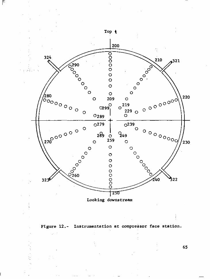
// “0 0 0” \\ // -0 0 o- ’

// * u A

/I/

n ” 0 ,A” \

” \\ 0 0 0 39n \\ --- LO”

//h 0 209 0 A\22o -“oo

OO O” 0

a29s” 0289 I

0279 +

0 I -no 00° 2i?9 0

0 259 0

0 0 0 0

0

0

Looking downstream

Figure 12.- Instrumentation at compressor face station.

65

Configuration 1

Configuration 2

O-Low %I h Y Z-High 'k

01 I

cD Configuration 4

-.02r

-.Ol -_,O c

o 0

oow .

Configuration 5 -.02r

-.Ol c 1

0’1 I I I I

.4 . . . *0 Figure 13. - Zero-shift corrections to drag coefficient.

66

: .4 .I., -~:,6; ,. .7.,;. , -.8 I .g ,-1.0 A, /Ai

Figure lb..- Total inlet drag.

67

.

CD

.

.3

.2

.l .4 .5 .6 .7 .8 .9 1.0

Aoh. 1

Figure lb.- Continued.

68

69

.4

.3

cD

Figure l5.- Effect of Mach number on total inlet drag at Ao/Ai = 1.0.

70

.08

.06

CF

.04

. 02

0 0 .4 .8 1.2 1.6

Figure 16. - Estimated cowl skin friction drag coefficient.

cD

.2

1 .4 .5 .U

A,/Ai

.

Figure 17.- Effect of Reynolds number on total Inlet drag. Config. 2.

72

Aoh. (a) MO'= 0.55

Figure lg.- Inlet pressure recovery and distortion. 73

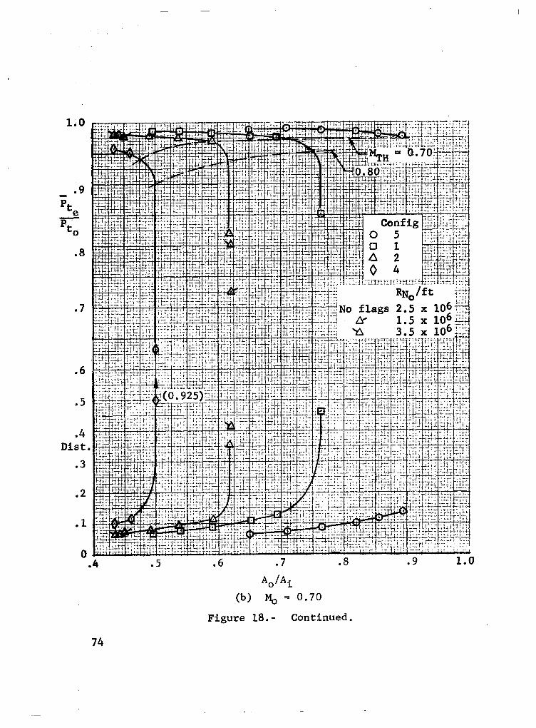
.6

.4 Dist

.3

Ao/Ai (b) M. = -0.70

Figure 18.0 Continued.

74

% e

Dis

Ao/A. 1 (c) MO = 0.85

Figure 18.0 Continued. 75'

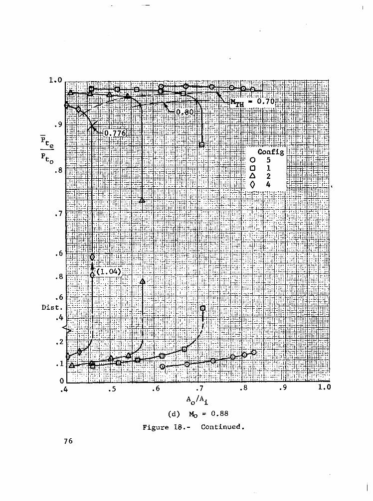
% e

Pt* .8

.6

Dis

.6 .7 .8 Ao/Ai

(d) I$, = 0.88

Figure 18.0 Continued.

.9 1.0

76

Dis

Ao/Ai (e) Q = 1.20

Figure 18.0 Continued. 77

Di

.5 .6 .7 .8 .9 1.0

78

Ao/Ai (f) Mo = 1.39

Figure 18.0 Concluded.

Nacelle station, in. Figure 19.0 Effect of capture area ratio on ramp centerline

pressure distribution, Config. 1, M. = 0.85.

79

.-

.8

.7

.6

5 .

.4

.3 CP

.2

.1

0

-. 1

-. 2

-. 3

-. 4

Figure 20.0 Effect of ramp angle on ramp centerline pressure distribution, M, = 0.85.

80

.a

.7

.6 CP

.5

.4

.3

.2

.l

0 1 2 3 4 5 6 7 8 9 fi 11 Nacelle station, in.

Figure 21.- Effect of Mach number on ramp centerline pressure distribution, Config. 1.

81

.6

.4

ep .2

0

-. 2

-. 4

82

1.64 In. Off ' Centerline Centerline A0 /Ai

l 0 .715 A -579 a .448

b 1 2 3 4 5 6 7 8 9 10 rL Inches From Leading Edge

Figure 22. - Comparison between centerline and off- centerline ramp pressure distributions, Config. 1, M. = .85.

-. 6

-. 8

---A--L __--- ----- 4

:.

: .,

16 18 " 20 Nacelle station, in.

Figure 23.- Effect of capture area ratio.on cowl lower denterline pressure distribution, Config. 1, M. = 0.85.

83

-. 6

-* 8

Nacelle station, in.

Figure 24.- Effect of ramp angle on cowl lower centerline pressure distribution, M. = 0.85. .'5

84

A\, I ----------A----- --- --i

I

- 5

.C

: ;

.2

0

-. 2

CP

-. 4

-. 6

-. 8

16 18 . 20 Nacelle station, in.

Figure 25,~ Effect of Mach number on cowl lower centerline pressure distribution, Config. 1.

85

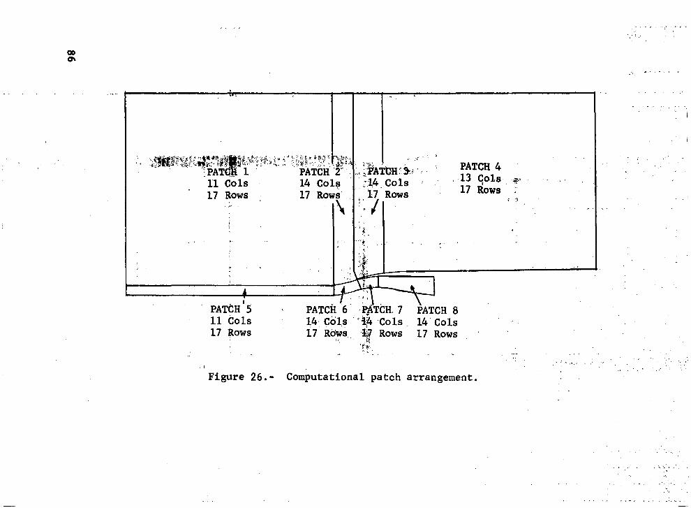
. . . ,. I I

‘.. i ,.

. .

1'1 Cols 14 Colg ,17 Rows ‘ 17 Roy W!

.,.

. . . .

.

A

> PATCH 4

I 13 qo1s,, Q' > 17 Rows :

i' :\

PATCH'5 11 601s 14: Co‘l.~ ';$I fols 14'Cols 17 qows 17 Rdys,, ,%# Rows 17 Rows .

'."*' . . _ CL -.. I. .. _: ,,,, i ,,: : i '. _. .: Figure 26.- Computational patch arrangement.

_ _,.. ~ ,‘_.,. ,: . .._

I ..’ ‘, .’ I.,

i . . - ;.:,“ .‘,..,I .’ -

:.:. ‘,

. . . .s.:‘: ..,, :”

..: . . s ,. .’

<,;‘;-J

:‘. .:; .,I _, . _,_ , . .I’, .

.

,‘$,:,;.:: 1

Figure 28.- Computational cell arrangement near inlet.

88 :, 3.

i I ! I i / \ \ : .‘\ - \ T \

Figure 29.- Computational cell arrangement near cowl lip.

89

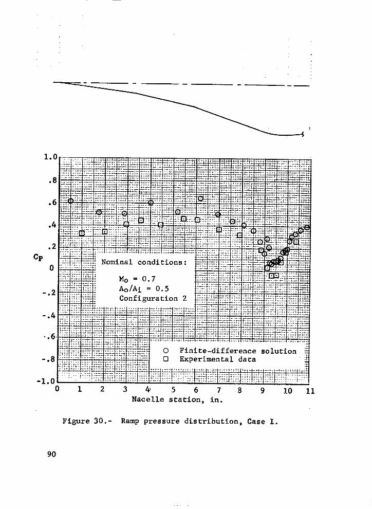
-1

0 Finite-difference solution - Experimental data

..l._,. . . . . . . . 1, .-_‘. . . . . : ._. :s;i:..;: . ..J.:::.

0 1 2 3 4 5 6 7 8 9 10 11 Nacelle station, in.

Figure SO.- Ramp pressure distribution, Case I.

90

I .

.8

.6

.4

.2

0

-. 2

CP -. 4

-. 6

-. 8

-1.0

-162

-1.4

-1.6

Figure 3f.- Cowl external pressure distribution, Case I.

91

.8

CP 0 Configuration 2

-9 2

-* 4

-. 6

-9 8

-1.0

-.1.2 8.6 8.7 8.8 8.9 .. 9.0 9.1

Nacelle station, in.

Figure 32.- Cowl lip internal pressure distribution, Case I.

92

Nominal conditions:

uo-0.7

Percent of input captured flow

Aohi - 0.5 Configuration 2

. .

Figure 33.- ,. Computed flow field streamlines, Case 1.

.,,. . C... I . 1, ., 1::

6 a :,,. ..,; - ,, ,‘..,l,‘, !. .,

‘;‘,‘,‘,, ‘I. ,;:‘: ,,..., ._ ,:. .‘. ._‘,

I &.. , _ I *_.,

1. ,. , .*: .

b

. . ., .,:

I. :,

1

. c ’

.

Figure 35.:~.~:; Reyised coniputational cell arrangement j +A . 3:'9, near inlet.

9s

96

III I I I 7

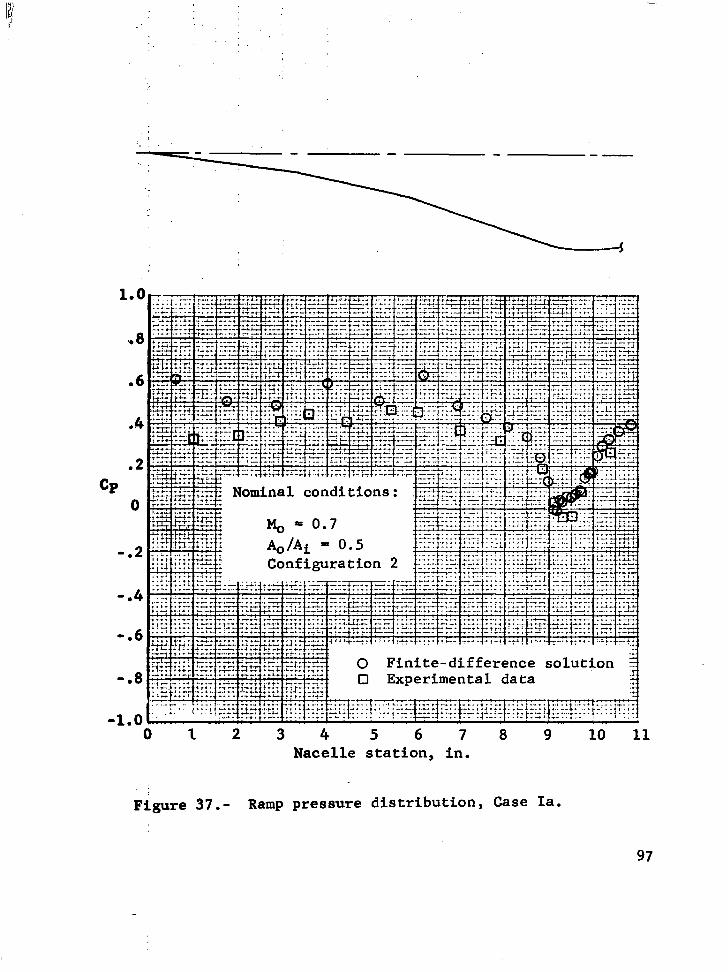
I$ -

1

CP

-

-1

. . 0

..8

.6

.4

Nominal conditions:

l 2

.4

.6

.8

-n 0 I2 3 4 5 6 7 8 9 l0l.l

Nacelle station, in.

Figure 37.- Ramp pressure distribution, Case Ia.

97

-. b

.‘..‘. ,. 1

4 I . : * .‘ .’

.I ‘..’ :.,

; . ,’ . ..’ . . 8 ‘.. .’

*. .

i ;,:. _’ ‘:‘. .,-. ,,. . .

T : j

;

. ‘. \

\

A?-- --.----‘-A m--L i- --I

I

.8

.6

.4

.2

-. 2

%? -. 4

-0 6

-. 8

-1.0

j'-$ -1.2

-1.6 10 11 12 13 14 Nacelle station, in.

Figure 38.- ,Cowl external pressure distribution, Case Ia.

98

1

-.

‘.,

. . . , :. , .-‘,..;-’ ‘.

_. _ ,. 1 -‘. . ! ,.. ‘,.

‘,a

.‘. I

: _.

I ,i ‘.s

1

.

f\ ‘hi.

,: :

,

’ ..

: ‘.’ ”

:_ ] .,:-j;~::;,,y .) .:: ,, .I..

‘1. : ‘.) , .,-i: ‘-,

ii3 :ta let' Nacelle Station 9.6 on the Lower Cowi

,,

,’ :

’ ,,’ .1

1

.,, .) ,.

:.

Y.’

k--Mesh Revised at

. .,, .-

0 .: Time Pass .', .

,. .;; .: 's ! , Flkgure 39',Effect of Mesh Change on b '

COW1 Pressure . -- .' ..l.' 99

II

i

.6

.4

.2

CP 0

-0 2

-m 4

-. 6

- '. 8

-1.0

-1.2 8“.6

.m Nominal conditions: ;-I;fii

M, = 0.7

A,/Ai = 0.5 Confirmration 2 ~&$~i~~

0 Finite-difference solution c3 Experimental data

a.7 8.8 8.9 9.0 9.1 Nacelle station, in.

Fig&-e 4Q.-, Cowl lip internal pressure distribution, C&e fa.

100

.8

.6

-. 2

-. 4 CP

-. 6

-. 8

-1.0

-1.k

-1.8 01 2 3 4. 5 6 7 8 9 i8 11

Nacelle station, in.

Figure 41-.- Ramp pressure distribution, Case II. - / : c A.. *; .

101

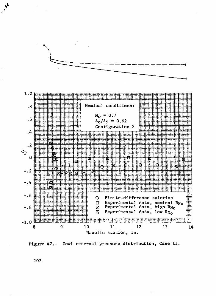
.8

.6

.4

.2

CP 0

-. 2

-. 4

-. 6

-. 8

-1;0

Nominal conditions:

M, = 0.7 Ao/Ai = 0.62 Configuration 2

0 Finite-difference solution 0 Experimental data, nominal RNo 0 Experimental data, high RN0 61 Experimental data, low RNn

8 9 10 11 12 Nacelle station, in.

13 14

Figure 42.- Cowl external pressure distribution, Case II.

102

.8

.6

.2

cP O

-. 2

-. 4

-9 6

-. 8

-1,o

-1.2

inal conditions:

!+r-tt+l

M, - 0.7 A0 /Ai = 0.62 Configuration 2

ifftT:~:'+fni'rf.~.~!r,~It:t~-; i 0 Finite-difference solution 0 Experimental data, nominal RN0 q Experimental data, high RN0 6l Experimental data. low RN,

8.8 8.9 9.0 9.1 Nacelle station, in.

Figure 43.- Cowl lip internal pressure distribution, Case II.

103

(a)\ Flow geometry

Patch Patch

0 2 0 3

Patch

0 1 L 4

(b) .-Mesh patch arrangement

Boundary 47

Boundary -Shared - Patch c/2

0 2 Boundary 0 3

i Boundary 3> Boundary 32 Shared Bounda 1

v 47 1

Patch 0 1

Boundary e

(c) Patch boundary nomenclature

.i l?i‘gur& 44. - Example mesh-patch arkangement.

104

:

I .

i . . .

(a) Inlet flow field

0 1

(b) Non-lifting airfoil

(c) Lifting airfoil

Figure 45.- Sample mesh-patch arrangement. 105

I

:.

,,’ ;:.;;

:, .: .. .

-. . . ‘..C_

.,:’ :’ ~ , . : !;

- ,. .’ . .

‘,’ : ... ;.. ,I*

. .‘_ .?,.I -3 . ‘.

8 . ..:;i ., .

. .

2

:i.-

Figure 46.- Sample computer-generated me+!geoqetry. . 106 _ .,I.

1.; *U.S. GOVERNMENT PRINTING OFFICE: 1976 - 635475195 . .I .