This is a repository copy of Infinite-dimensional Lie algebras determined by the space of symmetric squares of hyperelliptic curves.

White Rose Research Online URL for this paper:http://eprints.whiterose.ac.uk/123925/

Version: Accepted Version

Article:

Buchstaber, VM and Mikhailov, AV (2017) Infinite-dimensional Lie algebras determined by the space of symmetric squares of hyperelliptic curves. Functional Analysis and Its Applications, 51 (1). pp. 2-21. ISSN 0016-2663

https://doi.org/10.1007/s10688-017-0164-5

(c) 2017, Springer Science+Business Media New York. This is an author produced version of a paper published in Functional Analysis and Its Applications. Uploaded in accordance with the publisher's self-archiving policy. The final publication is available at Springer via https://doi.org/10.1007/s10688-017-0164-5

eprints@whiterose.ac.ukhttps://eprints.whiterose.ac.uk/

Reuse

Items deposited in White Rose Research Online are protected by copyright, with all rights reserved unless indicated otherwise. They may be downloaded and/or printed for private study, or other acts as permitted by national copyright laws. The publisher or other rights holders may allow further reproduction and re-use of the full text version. This is indicated by the licence information on the White Rose Research Online record for the item.

Takedown

If you consider content in White Rose Research Online to be in breach of UK law, please notify us by emailing eprints@whiterose.ac.uk including the URL of the record and the reason for the withdrawal request.

Infinite-Dimensional Lie Algebras Determined by the

Space of Symmetric Squares of Hyperelliptic Curves∗

V. M. Buchstaber and A. V. Mikhailov

November 12, 2017

Abstract

We construct Lie algebras of vector fields on universal bundles of symmetric squares of

hyperelliptic curves of genus g = 1, 2, . . . . For each of these Lie algebras, the Lie subalge-

bra of vertical fields has commuting generators, while the generators of the Lie subalgebra

of projectable fields determines the canonical representation of the Lie subalgebra with

generators L2q, q = −1, 0, 1, 2, . . . , of the Witt algebra. As an application, we obtain

integrable polynomial dynamical systems.

Introduction

The connection of the theory of infinite-dimensional Lie algebras with the classical theory ofsymmetric polynomials [1] and the modern theory of integrable systems is widely known andfruitful (see [2]). In this article we obtain a description of the Lie algebras G(E2

N,0) of vectorfields on the spaces of the universal bundles E2

N,0 (see Definition 2) of the symmetric squares ofthe hyperelliptic curves

Vx=

{(X, Y ) ∈ C

2 : Y 2 =N∏

i=1

(X − xi)

}, x = (x1, . . . , xN).

The Lie algebra G(E2N,0) contains the Lie subalgebra of fields lifted from the base SymN(C)

(such fields are said to be base), i.e., horizontal and projectable fields (see [3] and [4, p. 337])over the polynomial Lie algebra G(SymN(C)) (see [5], [6]) of derivations of the ring of symmetricpolynomials in x1, . . . , xN . Lie algebras with such a structure form an important class of Liealgebroids; see [7].

The Lie algebra G(SymN(C)) naturally arises and plays an important role in various areas ofmathematics and mathematical physics, including the isospectral deformation method and theclassical method of separation of variables. In fundamental works (see, e.g., [5] and [8]) ascoordinates on SymN(C) the elementary symmetric functions e1, . . . , eN were chosen. In [5], interms of the action of the permutation group SN on C

N , the operation of convolution of invari-ants was introduced and basis vector fields on SymN(C) were defined, which are independent atany point of the variety of regular orbits. At each point of the variety of irregular orbits these

∗The work was supported by the Royal Society International Exchanges Scheme Grant.

1

fields generate the tangent space to the stratum of the discriminant hypersurface containing thegiven point. Zakalyukin’s well-known construction yields basis vector fields Vi =

∑Vi,j(e)

∂∂ej

,

e = (e1, . . . , eN), with symmetric matrix Vi,j, which are tangent to the discriminant.

In this article we show that the use of the Newton polynomials p1, . . . , pN makes it possibleto substantially simplify the formulas and, most importantly, employ the remarkable infinite-dimensional Lie subalgebra W−1 of the Witt algebra W in computations. The generators of theLie algebraW−1 are L−2, L0, L2, . . . , and the commutation relations have the form [L2q1 , L2q2 ] =2(q2 − q1)L2(q1+q2).

For any N , the Lie algebra W−1 has a faithful canonical representation in the Lie algebraG(SymN(C)) which maps the generator L2q to the Newton field L0

2q = 2∑xq+1i ∂xi

. The imageof this representation belongs to the Lie algebra W−1(N), which has the structure of a free leftmodule over the polynomial ring C(SymN(C)). We obtain an explicit expression for the vectorfields Vi with symmetric matrix Vi,j(e) in terms of the Newton fields L0

2q (see Corollary 7). Animportant role in our calculations is played by a grading of variables and operators. In thisconnection, we introduce variables y2m and N2k by setting em = y2m and pk = N2k and bear inmind that deg xi = 2.

Note that the Jacobi identity in the C[N2, . . . ,N2N ]-polynomial Lie algebra W−1(N) impliesthe nontrivial differential relation

N∑

m=1

m

(N2(k+m)

∂N2(q+n)

∂N2m

−N2(q+m)

∂N2(k+n)

∂N2m

)= (q − k)N2(k+q+n)

for the Newton polynomials. We show that there exists a unique representation of the Liealgebra W−1 in the Lie algebra of horizontal vector fields L−2, L0, L2, . . . of the Lie algebroidG(E2

N,0) (see Theorem 6). The proof of the uniqueness of this representation uses the fact that,relative to the Lie bracket [·, ·], the Lie algebra W−1 is defined by the generators L−2 and L4

and the relation [L2, [L2, [L2, L4]]] = 12[L4, [L2, L4]].

On the Lie algebroid G(E2N,0) there exist two commuting vertical vector fields. For each point

x, the restrictions of these fields to Sym2(Vx) are the images of obviously commuting fields on

Vx× V

x. In our upcoming publication we shall give an explicit description of such commuting

fields on Symk(Vx) for any k ≥ 2. In Section 4 of this article we give an explicit description of

these fields in the case of interest to us, namely, for k = 2.

Similar operators on Symm(C2) were constructed in [9] on the basis of a construction of thespectral curve and the Poisson structure. A proof of the commutativity of operators in [9] usesa method that differs from ours.

The key results of our work are a formula for the generating series L(t) (see Theorem 7) ofthe horizontal vector fields L0

−2, . . . ,L02k, . . . that determine a representation of the Lie algebra

W−1 and a commutation formula for the vertical and horizontal vector fields (see Theorem 8).

In Section 6 we construct an N -dimensional algebraic varietyW (N) in the (N+2)–dimensionalalgebraic variety E2

N,0 and homeomorphisms fN : CN+2 \ {u4 = 0} → E2N,0 \W (N), where {u4 =

0} is a hyperplane in CN+2 with graded coordinates u2, u4, vN−2, vN ; y2, . . . , y2(N−2). One of the

main results of the present work is an explicit construction, which uses the homeomorphismsfN , of the polynomial Lie algebras on C

N+2 that are determined by the Lie algebroids G(E2N,0),

N = 3, 4, . . . (see Theorem 9).

The article concludes with a description of polynomial Lie algebras on CN+1 for N = 3, 4, 5.

In the case N = 5, we obtain a polynomial Lie algebra isomorphic to the Lie algebra of vector

2

fields on the universal bundle of Jacobians of nonsingular hyperelliptic curves of genus 2, whichwas constructed in [10] by using the theory of two-dimensional σ-functions.

1 The Space of Symmetric Squares of Hyperelliptic

Curves

Consider a family of plane curves

VN,0 = {(X, Y ;x) ∈ C2 × C

N : π(X, Y ;x) = 0}, (1)

where

π(X, Y ;x) = Y 2 −N∏

k=1

(X − xk). (2)

The vector ξN(x) = e is the parameter set for a curve in family (1). By VN we denote thesubfamily of curves satisfying e1 = p1 = 0.

In this paper we use the following grading of variables: deg xk = 2, k = 1, . . . , N , degX = 2,and deg Y = N . With respect to this grading the polynomial π(X, Y ;x) is homogeneous ofdegree 2N .

The discriminant variety of family (1) is the algebraic variety

Disc(VN,0) = {ξN(x) ∈ SymN(C) : ∆N = 0}, where ∆N =∏

i<j

(xi − xj)2.

The discriminant variety Disc(VN) of the family of curves VN is defined similarly. The varietyDisc(VN,0) ⊂ C

N is the image under the projection CN → SymN(C) = C

N of the union of theso-called mirrors, that is, the hyperplanes {xi = xj, i 6= j}, and Disc(VN) ⊂ C

N−1 is the imageof the intersection of the space C

N−1 = {e ∈ Cn : e1 = 0} with the union of mirrors.

For N = 3, the variety Disc(V3) ⊂ C2 in the coordinates (e2, e3) is determined by the equation

∆3 = 27e23 − 4e32 = 0, i.e., is the well-known swallowtail in C2. In the book [5] it was proposed

to refer to the varieties Disc(VN) as generalized swallowtails in CN−1.

Let BN,0 and BN denote the open varieties CN \Disc(VN,0) and CN−1 \Disc(VN), respectively.

The curves of the families VN,0 and VN with parameters in the spaces BN,0 and BN are said tobe nonsingular for obvious reasons. They have genus

[N−12

]. For example, in the cases N = 3

and 4, these are elliptic curves.

We set EN,0 = {(X, Y ;x) ∈ C2 × C

N : π(X, Y ;x) = 0, ξ(x) ∈ BN,0}. The group SN acts freely

on EN,0 by permutations of the coordinates x1, . . . , xN , and therefore a regular N !-sheeted

covering EN,0 → EN,0 = EN,0/SN is defined.

Definition 1 The universal bundle of nonsingular hyperelliptic curves of family (1) is thebundle EN,0 → BN,0 : (X, Y ; ξ(x)) 7→ ξ(x).

The space EN,0 is the universal space of nonsingular hyperelliptic curves of genus[N−12

]. The

fiber over a point of the base BN,0 is the curve with parameters determined by this point. Theuniversal bundle EN → BN of nonsingular hyperelliptic curves is defined similarly.

3

We set

E2N,0 = {(X1, Y1;X2, Y2;x) ∈ C

2×C2×C

N : π(Xk, Yk;x) = 0, k = 1, 2; X1−X2 6= 0, ξ(x) ∈ BN,0}.

The group G = S2 × SN acts freely on E2N,0, so that the generator of S2 determines the permu-

tation (X1, Y1) ↔ (X2, Y2), and the elements of the group SN determine permutations of the

coordinates of the vector x. Therefore, a regular covering E2N,0 = E2

N,0/G→ E2N,0 is defined.

Definition 2 The universal bundle of symmetric squares of nonsingular hyperelliptic curves offamily (1) is the bundle

E2N,0 → BN,0 : ([X1, Y1;X2, Y2]; [x]) 7→ [x],

where [X1, Y1;X2, Y2] = ξ2(X1, Y1;X2, Y2), [x] = ξ(x), and ξ2 : C2 × C

2 → Sym2(C2) is thecanonical projection onto the symmetric square of C2.

The space E2N,0 is called the universal space of symmetric squares of nonsingular hyperelliptic

curves of genus[N−12

]. The fiber over a point of the base BN,0 is the variety (Sym

2V )\(X1−X2 =0) with parameters determined by this point.

The universal bundle E2N → BN is defined similarly.

2 The Lie Algebra of Newton Vector Fields

In the paper [6] the theory of polynomial Lie algebras was constructed. Important examplesof such infinite-dimensional Lie algebras are the Lie algebras of vector fields on C

N and CN−1

tangent to the varieties Disc(VN,0) and Disc(VN) and, therefore, the Lie algebras of vector fieldson BN,0 and BN .

In this section we give an explicit description of the Lie algebras GP0(N) and GP (N) of vector

fields in coordinates (p1, . . . , pN) and (p2, . . . , pN) determined by the Newton polynomials. Wehave deg xi = 2, i = 1, . . . , N . To control grading, we introduce the notation

N2k = pk(x) =N∑

i=1

xki , k = 0, 1, . . . .

For graded generators of the polynomial ring P(SymN(C)) we take the polynomialsN2, . . . ,N2N . Then P(SymN(C)) ≃ C[N2, . . . ,N2N ].

Definition 3 The gradient homogeneous polynomial vector fields

L02q = 2

N∑

i=1

xq+1i ∂xi

, q = −1, 0, 1, . . . , (3)

on CN of degree 2q are called the Newton derivations of the ring C[x1, . . . , xN ].

Lemma 1 The operators L02q, q = −1, 0, 1, . . . are derivations of the ring C[N2, . . . ,N2N ], and

they are uniquely determined by the formula

L02qN2k = 2kN2(k+q), k = 1, 2, . . . . (4)

4

Corollary 1 The operators L02q act on the ring C[N2, . . . ,N2N ] as

L02q =

N∑

k=1

2kN2(q+k)∂

∂N2k

. (5)

Lemma 1 and Corollary 1 are verified directly.

Let us write the equation∏N

i=1(x− xi) = 0 in the form xN =∑N

j=1(−1)j+1y2jxN−j.

Lemma 2 For any k ≥ 0,

xN+k =N∑

j=1

(−1)j+1y2k,2jxN−j, (6)

where the {y2k,2j, k = 1, . . . }, j = 1, . . . , N , are the sets of symmetric functions in x1, . . . , xNwith generating series

Y2j =∞∑

k=0

y2k,2jtk =

1

E(t)

N−j∑

s=0

(−1)sy2(j+s)ts, E(t) =

N∏

i=1

(1− xit). (7)

Proof: According to (6), for any k ≥ 0, we have

N∑

j=1

(−1)j+1y2(k+1),2jxN−j = xN+k+1 = x · xN+k

= y2k,2

[ N∑

j=1

(−1)j+1y2jxN−j

]+

N∑

j=2

(−1)j+1y2k,2jxN−j+1.

Hence y2(k+1),2N = y2Ny2k,2 and y2(k+1),2j = y2jy2k,2 − y2k,2(j+1). We obtain the following systemof equations for the generating series:

Y2N = y2N(1 + tY2),

Y2j = y2j(1 + tY2)− tY2(j+1), j = 1, . . . , N − 1.

Solving this system, we obtain (7).�

Corollary 2 For any k ≥ 0,

N2(N+k) =N∑

j=1

(−1)j+1y2k,2jN2(N−j), (8)

L02(N+k−1) =

N∑

j=1

(−1)j+1y2k,2jL02(N−j−1). (9)

Let us introduce the generating series L0(t) =∑∞

q=−1 L02qt

q+1.

Corollary 3 The following relation holds:

L0(t) =1

E(t)

N∑

m=1

E(t;m)L02(m−2)t

m−1, (10)

where

E(t;m) =N−m∑

k=0

(−1)ky2k tk and E(t) = E(t; 0). (11)

5

Poof Let us write the series L0(t) in the form L0(t) =∑N−2

q=−1 L02qt

q+1 + tN∑∞

k=0 L02(N+k−1)t

k.

According to (9), we obtain

L0(t) =N−2∑

q=−1

L02qt

q+1 + tNN∑

j=1

(−1)j+1

( ∞∑

k=0

y2k,2j tk

)L0

2(N−j−1)

=N∑

j=1

tN−j(1 + (−1)j+1tjY2j)L02(N−j−1).

It remains to use (7).�

Lemma 3 The following relation holds:

[L02q1,L0

2q2] = 2(q2 − q1)L

02(q1+q2)

. (12)

Proof: The required relation follows directly from (4).�

Corollary 4 For all k, q ∈ N and n = 1, . . . , the polynomials N2k, k = 0, 1, . . . , are related by

N∑

m=1

m

(N2(k+m)

∂N2(q+n)

∂N2m

−N2(q+m)

∂N2(k+n)

∂N2m

)= (q − k)N2(k+q+n). (13)

Proof: The required relations follow directly from (5) and (12).�

Example 1 For N = 3, the polynomials N2, N4, and N6 are algebraically independent andN0 = 3. For k = 0, q = 1, and n = 3, relation (13) gives the Euler differential equation

2N2∂N8

∂N2

+ 4N4∂N8

∂N4

+ 6N6∂N8

∂N6

= 8N8.

Lemma 4 For all q = −1, 0, 1, . . . ,

L02q∆(N) = 4γ2q(N)∆(N), (14)

where

∆(N) =∏

i<j

(xi − xj)2 and γ2q(N) =

∑

i<j

xq+1i − xq+1

j

xi − xj. (15)

For any k ≥ 0,

γ2(N+k)(N) =N−1∑

s=1

(−1)s+1y2(k+1),2sγ2(N−s−1).

Proof: We have

L02q∆(N) = 4∆(N)

N∑

k=1

xq+1k ∂k ln

∏

i<j

(xi − xj) = 4∆(N)

(∑

i<j

xq+1i − xq+1

j

xi − xj

).

The formula for γ2(N+k)(N) follows from (6).�

6

Example 2 γ−2(N) = 0, γ0(N) = 2N(N − 1), and γ1(N) = 4(N − 1)N2.

Corollary 5 The vector fields L02q, q = −1, 0, 1, . . . , on C

N determine vector fields on SymN(C)

tangent to the algebraic variety Disc(VN,0) ⊂ SymN(C).

Theorem 1 The Lie algebra GP0(N) of vector fields on the variety BN,0 in the coordinates

N2, . . . ,N2N has the structure of a free N-dimensional module over the ring C[N2, . . . ,N2N ]with generators L0

2q, q = −1, 0, 1, . . . , N − 2. The set of generators extends to an infinite set{L0

2q}, where the elements L02q for q > N − 2 are given by (9). The operators L0

2q act on N2k

by (4).

The structure of the Lie algebra GP0(N) is determined by (12) and (4), where the N2k for k > N

are the polynomials N2k(N2, . . . ,N2N) defined recursively by (8).

We set L0A(t) = tE(t)L0(t). According to Corollary 3, operators L0

A,2(k−2) for which

L0A(t) =

N∑

m=1

L0A,2(m−2)t

m =N∑

m=1

E(t;m)L02(m−2)t

m

are defined.

Lemma 5 The following relation holds: L0A(t) =

∑N

k=1 t∏

j 6=k(1− xjt)∂

∂xk.

Proof: We have

L0A(t) = tE(t)

∞∑

q=−1

L02qt

q+1 = E(t)N∑

k=1

t

1− xkt

∂

∂xk=

N∑

k=1

t∏

j 6=k

(1− xjt)∂

∂xk. �

�

Example 3 L0A,−2 = L0

−2 and L0A,2(N−2) = y2NL

0−4.

Lemma 6 The generating polynomial

L0A(t)E(s) =

N∑

m=1

(−1)m(LA(t)y2m)sm

in s is symmetric with respect to the permutation t↔ s.

Proof: We have

L0A(t)E(s) = tE(t)L0(t)E(s) = −E(t)E(s)

N∑

i=1

t

1− xit

s

1− xis. �

�

Corollary 6 The action of the operators L0A,2(k−2), k = 1, . . . , N , on the elementary symmetric

polynomials em = y2m is given by a symmetric matrix T 0k,m = T 0

k,m(y2, . . . , y2N), that is,

L0A,2(k−2)y2m = L0

A,2(m−2)y2k.

7

Proof: We have

L0A(t)E(s) =

( N∑

k=1

(−1)kL0A,2(k−2)t

k

)( N∑

m=1

(−1)my2msm

)

=N∑

k=1

N∑

m=1

(−1)k+m(L0A,2(k−2)y2m)t

ksm.

It remains to use Lemma 6.�

The Lie algebra GP (N) of vector fields on BN in the coordinates N4, . . . ,N2N is a Lie subalgebraof GP0

(N). It consists of the fields that leave the ideal J2 = 〈N2〉 ⊂ C[N2, . . . ,N2N ] invariant.

We have L0−2N2 = 2N and L0

2qN2 = 2N2(q+1). We set L0 = L00 and L2q = L0

2q −1NN2(q+1)L

0−2.

By construction L0N2 = 2N2 and L2qN2 = 0 for q 6= 0.

Theorem 2 The Lie algebra GP (N) of vector fields on BN in the coordinates N4, . . . ,N2N hasthe structure of a free (N−1)-dimensional module over the ring C[N4, . . . ,N2N ] with generatorsL2q, q = 0, 1, . . . , N−2. The set of generators extends to an infinite set {L2q}, and the elementsL2q for q = N + k − 1, k ≥ 0, are given by (see (9))

L02(N+k−1) =

N∑

j=1

(−1)j+1y2k,2jL02(N−j−1), (16)

where y2k,2j ≡ y2k,2j mod 〈N2〉 and the y2k,2j are the polynomials determined by the generatingseries (7).

The structure of the Lie algebra on GP (N) is introduced directly by the condition that this is aLie subalgebra of the Lie algebra GP0

(N).

Let LA(t) = tE(t)L(t), where

L(t) =∞∑

q=−1

L2qtq+1 =

∞∑

q=−1

(L2q −

1

NN2(q+1)L

0−2

)tq+1.

Lemma 7 The following relation holds:

LA(t) = L0A(t) +

1

N

(L0

−2E(t)

)L0

−2 =

[L0 −

(1−

4

N

)y2L−2

]t2 + · · · . (17)

Lemmas 6 and 7 give the following result.

Lemma 8 The generating polynomial LA(t)E(s) =∑N

m=1(−1)m(LA(t)y2m)sm is symmetric

with respect to the permutation t↔ s.

Let us introduce operators L0A,2(k−2) such that LA(t) =

∑N

k=2 LA,2(k−2)t.

Corollary 7 The operators LA,2(k−2), k = 2, . . . , N , leave the ideal 〈N2〉 invariant. Theiraction on the elementary symmetric polynomials em = y2m is determined up to the ideal 〈N2〉by a symmetric matrix Tk,m = Tk,m(y4, . . . , y2N).

8

Proof: The proof of this assertion is similar to that of Corollary 6.�

The Lie algebra GP (N) of vector fields on BN in the coordinates y4, . . . , y2N has the structureof a free (N − 1)-dimensional module over the ring C[y4, . . . , y2N ] with generators LA,2(k−2),k = 2, . . . , N . The action of these generators on y2m is given by a symmetric matrix (Tk,m) =(Tk,m(N)).

Remark 1 For each N , we give an explicit construction of the fields LA,2(k−2) and the sym-metric matrix (Tk,m(N)). The notation LA is suggested by Arnold’s monograph [5] (see also[8]). These fields will be used in Section 9 to construct the Lie algebroids G(E2

N,0) and explicitlydescribe an isomorphism between the Lie algebroid G(E2

5,0) and the algebroid constructed in [10]from the universal bundle of Jacobians of genus 2 curves.

3 Representations of the Witt Algebra W−1 in Lie Al-

gebras

with the Structure of a Free N -Dimensional Module

over the Polynomial Ring

Let us introduce the following notion.

Definition 4 We define an N-polynomial Lie algebra W−1(N) as the graded Lie algebra with

• the structure of a free left module over the graded ring A(N) = C[v2, . . . , v2N ], deg v2k = 2k;

• an infinite set of generators L02q, q = −1, 0, 1, . . . , degL0

2q = 2q;

• a skew-symmetric operation [·, ·] such that

[L02q1, L0

2q2] = 2(q2 − q1)L

02(q1+q2)

,

[L2q1 , v2kL2q2 ] = v2q1,2kL2q2 + v2k[L2q1 , L2q2 ],

[v2k1L2q1 , v2k2L2q2 ] = v2k1v2q1,2k2L2q2 − v2k2 [L2q2 , v2k1L2q1 ],

where v2q,2k ∈ A(N) is a homogeneous polynomial v2q,2k(v2, . . . , v2N) of degree 2(q + k).

Using the identity vk1(vk2L2q) = (vk1vk2)L2q and Leibniz’ rule, we see that the skew-symmetricoperation [·, ·] on the Lie algebra W−1(N) is completely determined by the set of homogeneouspolynomials v2q,2k = v2q,2k(v2, . . . , v2N).

Theorem 3 The set of polynomials v2q,2k = v2q,2k(v2, . . . , v2N)∈A(N) determines a skew-symmetric operation on an N-polynomial Lie algebra W−1(N) if and only if the homomorphism

γ : W−1(N) → DerA(N), γ(L02q) =

N∑

k=1

v2q,2k∂

∂v2k,

of A(N)-modules is a homomorphism of the N-polynomial Lie algebraW−1(N) to the Lie algebraof polynomial derivations of the ring A(N) = C[v2, . . . , v2N ].

9

Proof: The theorem is proved by a direct verification of its statements.�

The Lie algebra W−1 with generators L02q, q = −1, 0, 1, . . . , contains the Lie subalgebra gen-

erated by the three operators L0−2, L

00, and L0

2, where [L0−2,L

02] = 4L0

0. The Lie algebra W−1

with respect to the bracket [·, ·] is generated by only two generators, L0−2 and L0

4.

Example 4 6L02 = [L0

−2,L04], 4L

00 = [L0

−2,L02], and 2L0

6 = [L02,L

04].

The generators L2q, where q ≥ 1, are given by the recurrence relation 2qL02(q+2) = [L0

2,L02(q+1)].

Moreover, the operators L0−2, L

04 are related by commutation relations, the first of which is

[L02, [L

02, [L

02,L

04]]] = 12[L0

4, [L02,L

04]]. (18)

Corollary 8 The representations γj(L02q) =

∑N

k=1 vj2q,2k

∂∂v2k

, j = 1, 2, of the N–polynomial

algebra W−1 coincide if and only if v12q,2k ≡ v22q,2k for q = −1 and 2.

By construction there is an embedding of the Lie algebra W−1 into the Lie algebra W−1(N).On the other hand, the ring homomorphism ϕ : A(N) → C, ϕ(vk) = 0, k = 1, . . . , N , inducesa projection W−1(N) → W−1 of Lie algebras.

Corollary 9 The homomorphism

γ : W−1(N) → GP,0(N), γ(L02q) = L0

2q =N∑

k=1

2kN2(q+k)∂

∂N2k

, γ(v2k) = N2k,

extends to an epimorphism of Lie algebras.

Note that the nontrivial relation (13) between Newton polynomials in x1, . . . , xN ensures thefulfillment of the condition

γ([L2k, L2k]) = [γ(L2k), γ(L2k)].

The kernel of the homomorphism γ is described by (9). The restriction of the homomorphismγ to the Lie subalgebra W−1 gives a representation of the Lie algebra W−1 in the Lie algebraGP,0(N) with the structure of a free N -dimensional C[N2, . . . ,N2N ]-module.

4 Commuting Vector Fields on the Symmetric Square

of a Plane Curve

Consider the symmetric square of the curve V = {(X, Y )∈C2 : F (X, Y )= 0}, where F (X, Y )

are polynomials in X and Y . Let Dk = F (Xk, Yk)Yk∂Xk

− F (Xk, Yk)Xk∂Yk

, k = 1, 2. Weintroduce the operators

L1 =1

X1 −X2

(D1 −D2), L2 =1

X1 −X2

(X2D1 −X1D2). (19)

10

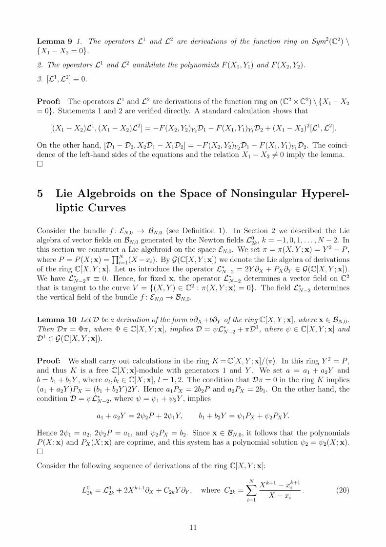
Lemma 9 1. The operators L1 and L2 are derivations of the function ring on Sym2(C2) \{X1 −X2 = 0}.

2. The operators L1 and L2 annihilate the polynomials F (X1, Y1) and F (X2, Y2).

3. [L1,L2] ≡ 0.

Proof: The operators L1 and L2 are derivations of the function ring on (C2 ×C2) \ {X1 −X2

= 0}. Statements 1 and 2 are verified directly. A standard calculation shows that

[(X1 −X2)L1, (X1 −X2)L

2] = −F (X2, Y2)Y2D1 − F (X1, Y1)Y1

D2 + (X1 −X2)2[L1,L2].

On the other hand, [D1 −D2, X2D1 −X1D2] = −F (X2, Y2)Y2D1 − F (X1, Y1)Y1

D2. The coinci-dence of the left-hand sides of the equations and the relation X1 −X2 6= 0 imply the lemma.�

5 Lie Algebroids on the Space of Nonsingular Hyperel-

liptic Curves

Consider the bundle f : EN,0 → BN,0 (see Definition 1). In Section 2 we described the Liealgebra of vector fields on BN,0 generated by the Newton fields L0

2k, k = −1, 0, 1, . . . , N − 2. Inthis section we construct a Lie algebroid on the space EN,0. We set π = π(X, Y ;x) = Y 2 − P ,

where P = P (X;x) =∏N

i=1(X−xi). By G(C[X, Y ;x]) we denote the Lie algebra of derivationsof the ring C[X, Y ;x]. Let us introduce the operator L∗

N−2 = 2Y ∂X + PX∂Y ∈ G(C[X, Y ;x]).We have L∗

N−2π ≡ 0. Hence, for fixed x, the operator L∗N−2 determines a vector field on C

2

that is tangent to the curve V = {(X, Y ) ∈ C2 : π(X, Y ;x) = 0}. The field L∗

N−2 determinesthe vertical field of the bundle f : EN,0 → BN,0.

Lemma 10 Let D be a derivation of the form a∂X+b∂Y of the ring C[X, Y ;x], where x ∈ BN,0.Then Dπ = Φπ, where Φ ∈ C[X, Y ;x], implies D = ψL∗

N−2 + πD1, where ψ ∈ C[X, Y ;x] andD1 ∈ G(C[X, Y ;x]).

Proof: We shall carry out calculations in the ring K =C[X, Y ;x]/〈π〉. In this ring Y 2 = P ,and thus K is a free C[X;x]-module with generators 1 and Y . We set a = a1 + a2Y andb = b1 + b2Y , where al, bl ∈ C[X;x], l = 1, 2. The condition that Dπ = 0 in the ring K implies(a1 + a2Y )PX = (b1 + b2Y )2Y . Hence a1PX = 2b2P and a2PX = 2b1. On the other hand, thecondition D = ψL∗

N−2, where ψ = ψ1 + ψ2Y , implies

a1 + a2Y = 2ψ2P + 2ψ1Y, b1 + b2Y = ψ1PX + ψ2PXY.

Hence 2ψ1 = a2, 2ψ2P = a1, and ψ2PX = b2. Since x ∈ BN,0, it follows that the polynomialsP (X;x) and PX(X;x) are coprime, and this system has a polynomial solution ψ2 = ψ2(X;x).�

Consider the following sequence of derivations of the ring C[X, Y ;x]:

L02k = L0

2k + 2Xk+1∂X + C2kY ∂Y , where C2k =N∑

i=1

Xk+1 − xk+1i

X − xi. (20)

11

Theorem 4 The homogeneous fields L02k, k = −1, 0, 1, . . . , of degree 2k are uniquely deter-

mined by the condition that they are lifts of the Newton fields L02k and generate the Lie algebra

of Newton horizontal vector fields on the space of the bundle EN,0, that is,

[L02q1, L0

2q2] = 2(q2 − q1)L

02(q1+q2)

.

Proof: We set L02k = L0

2k+2Xk+1∂X = 2(∑N

i=1 xk+1i ∂xi

+Xk+1∂X). The operator L02k determines

a Newton derivation of the ring C[X;x]. It is easy to check that (20) can be written as

L02k = L0

2k +1

2(L0

2k lnP )Y ∂Y . (21)

Hence L02k(Y

2 − P ) = P (L02k lnP − L0

2k lnP ) ≡ 0. Thus, formula (20) determines horizontalvector fields L0

2k, k = −1, 0, 1, . . . , on EN,0, which are lifts of the fields L02k on the base BN,0.

Now let L0,12k and L0,2

2k be two homogeneous horizontal vector fields on EN,0 that are lifts ofthe field L0

2k on the base BN,0. Then, according to Lemma 10, L0,22k = L0,1

2k + ψ2k+2−NL∗N−2,

where ψ2k+2−N = ψ1 + ψ2Y and ψ1, ψ2 ∈ C[X;x] are homogeneous polynomials such thatdegψ1 = 2m = 2k + 2−N and degψ2 = 2(k + 1−N).

Note that the degree of the function ψ2k+2−N cannot be negative. Hence the condition ψ2k+2−N

6= 0 implies N ≤ 2k + 2. On the other hand, according to Corollary 6, the generators of thealgebra W−1 are completely determined by the operators L0

−2 and L04. As a result, we obtain

the following conditions: N ≤ 0 for k = −1, N ≤ 4 for k = 1, and N ≤ 6 for k = 2. In thecase where k = 2 and N = 5, we obtain degψ1 = 1, which contradicts degψ1 = 2m. Thus, wehave proved that the lift of the fields L0

2k, k = −1, 0, 1, . . . , is unique for N = 5 and N > 6.

It remains to consider the cases N = 3, 4, 6. As shown above, in the case N = 6, the lifts of thefields L0

−2 and L02 are unique, and any lift of L0

4 must have the form L04 + αL∗

4, where α ∈ C.A direct verification shows that the commutation relation (see (18)) in the Witt algebra holdsonly for α = 0. Thus, in the case N = 6, the lift of the fields L0

2k is unique. Similar argumentsshow that this is also true in the cases N = 3 and 4.

The commutation rule [L02q1, L0

2q2] = 2(q2 − q1)L

02(q1+q2)

follows from the fact that L02k is a

Newton operator and from (21). This completes the proof of the theorem.�

Corollary 10 The generating function for the operators (20) has the form

L0(t) = L0(t) +1

2(L0(t) lnP )Y ∂Y, where L0(t) = L0(t) + 2

1

1−Xt∂X . (22)

Consider the space CN+1 with the graded coordinates (X, Y ;N2, . . . ,N2(N−1)). Using the equa-tion Y 2 = P (X;x), we can identify the space EN,0 with an open dense subvariety in C

N+1.The Lie algebra of vector fields on EN,0 described above determines a polynomial Lie algebragenerated by the field L∗

N−2 and the fields L0−2, L

00, L

02, . . . , L

02(N−2).

Example 5 Case N = 3. The coordinates in C4 are X, Y , N2, and N4. We have

1

3N6 = −Y 2 +X3 −N2X

2 +1

2(N 2

2 −N4)X +

(1

2N2N4 −

1

6N 3

2

).

Using this formula, we obtain an explicit expression for the basis polynomial fields L∗1, L

0−2, L

00,

and L02 in C

4.

12

6 Coordinate Rings of Spaces of Symmetric Squares of

Hyperelliptic Curves

Consider the space C2×C2 with coordinates (X1, Y1) and (X2, Y2) graded as above, i.e., so that

degXk = 2 and deg Yk = N , k = 1, 2, and the space C5 with graded coordinates u2, u4, vN ,

vN+2, and v2N . Here the subscript corresponds to the degree of variables.

Lemma 11 The algebraic homogeneous map

ξ : C2 × C2 → C

5, ξ((X1, Y1), (X2, Y2)) = (u2, u4, vN , vN+2, v2N),

where u2 = X1 + X2, u4 = (X1 − X2)2, vN = Y1 + Y2, vN+2 = (X1 − X2)(Y1 − Y2), and

v2N = (Y1 − Y2)2, makes it possible to identify the algebraic variety (C2 × C

2)/S2 with thehypersurface in C

5 determined by the equation u4v2N − v2N+2 = 0.

Proof: The lemma is proved directly.�

For what follows we need the homogeneous polynomials a2k(u2, u4) of degree 2k determined bythe generating series

1

(1−X1t)(1−X2t)= a(t; u2, u4) =

∞∑

k=0

a2k(u2, u4)tk

= 41

(2− u2t)2 − u4t2= 1 + u2t+ (t2). (23)

In the notation of Lemma 11 we have

∞∑

k=0

(Xk1 +Xk

2 )tk =

1

1−X1t+

1

1−X2t= (2− u2t)a(t; u2, u4). (24)

Moreover,

∞∑

k=2

(X1 −X2)(Xk−11 −Xk−1

2 )tk−2

=∞∑

k=2

[(Xk1 +Xk

2 )tk−2 −X1X2(X

k−21 +Xk−2

2 )tk−2] = u4a(t; u2, u4), (25)

∞∑

k=0

(Y1 − Y2)(Xk1 −Xk

2 )tk = (Y1 − Y2)

[1

1−X1t−

1

1−X2t

]= vN+2ta(t; u2, u4). (26)

We have Y 2j = XN

j +∑N

k=2(−1)ky2kXN−kj . Hence

(Y 21 + Y 2

2 ) =1

2(v2N + v2N)

= (2a2N − u2a2N−2) +N−1∑

k=2

(−1)ky2k(2a2(N−k) − u2a2(N−k−1)) + (−1)N2y2N .

13

We also have

(X1 −X2)(Y21 − Y 2

2 ) = vNvN+2 = u4

(a2(N−2) +

N−2∑

k=2

(−1)ky2ka2(N−k−2)

),

(Y1 − Y2)(Y21 − Y 2

2 ) = vNv2N = vN+2

(a2(N−1) +

N−1∑

k=2

(−1)ky2ka2(N−k−1)

).

The graded coordinate ring R0(N) of the space E2N,0 in (C2 ×C

2 \ {X1 −X2 = 0})×BN,0 (seeSection 1) has the form

C[X1, Y1;X2, Y2; x1, . . . , xN ]/J,

deg xj = degXk = 2, deg Yk = N, j = 1, . . . , N, k = 1, 2,

where J = 〈π1, π2〉 is the ideal generated by the polynomials πk = πk(Xk, Yk;x). Let RG0 (N) ⊂

R0(N) denote the invariant ring of the free action of G on R0(N). Consider the graded ringR(N) = R0(N)/〈y〉, where y = x1 + · · · + xN . Let RG(N) ⊂ R(N) denote the invariant ringof the free action of G on R(N). We shall treat the ring RG(N) as the coordinate ring of theuniversal space E2

N .

Lemma 12 The ring RG(N) is isomorphic to the graded ring

RGU = C[u2, u4, vN , vN+2, v2N ,y]/J

G,

where y = (y4, . . . , y2N) and the ideal JG has Grobner basis

P2N+4 = v2N+2 − u4v2N ,

P2N+2 = vNvN+2 − u4

(a2N−2 +

N−1∑

k=2

(−1)ky2ka2(N−k−1)

),

P2N = v2N + v2N − (a2N − u2a2(N−1))−N−1∑

k=2

(−1)ky2k(2a2(N−k) − u2a2(N−k−1))− (−1)N2y2N ,

P3N = vNv2N − vN+2

(a2(N−1) +

N−1∑

k=2

(−1)ky2ka2(N−k−1)

).

The relation vNP2N+4 − vN+2P2N+2 + u4P3N = 0 holds.

Proof: The lemma follows easily from the relations obtained above.�

Let us introduce the ring A(N) = C[u2, u4, vN−2, vN , y], where y = (y4, . . . , y2(N−2)).

Lemma 13 The following ring homomorphism holds:

ϕ : RGU → A(N),

ϕ(u2k) = u2k, k = 1, 2, ϕ(vN) = vN , ϕ(y2k) = y2k, k = 2, . . . , N − 2,

ϕ(vN+2) = u4vN−2, ϕ(v2N) = u4v2N−2,

ϕ(y2(N−1)) = (−1)N−1

[vN−2vN − a2(N−1) −

N−2∑

k=2

(−1)ky2ka2(N−k−1)

],

ϕ(y2N) = (−1)N1

2

[(v2N + v2N)− (2a2N − u2a2(N−1))

−N−1∑

k=2

(−1)ky2k(2a2(N−k) − u2a2(N−k−1))

].

14

Proof: A direct verification shows that the homomorphism ϕ maps the ideal JG to 0.�

Corollary 11 The homomorphism ϕ[u−14 ] : RG

U [u−14 ] → A(N)[u−1

4 ] is an isomorphism.

Proof: The ring homomorphism

η : A(N)[u−14 ] → RG

U [u−14 ],

η(u2k) = u2k, k = 1, 2, η(vN) = vN , η(y2k) = y2k, k = 2, . . . , N − 2,

η(vN−2) = u−14 vN+2

is inverse to the homomorphism ϕ[u−14 ].

�

Consider the space CN+4 with the graded coordinates (u2, u4, vN , vN+2, v2N ;y) and the space

CN+1 with the graded coordinates (u2, u4, vN−2, vN , y). As mentioned above, the space E2

N canbe identified with the algebraic subvariety in C

N+4 determined by the equations P2N+k = 0,k = 0, 2, 4, N (see Lemma 12). We set

b2N(u2; y) =1

2N−1

(uN2 +

N−1∑

k=2

(−1)k2ky2kuN−k2 + (−1)N2Ny2N

).

Let Ws(N), s = 1, 2, denote the algebraic subvarieties in CN+4 determined by the equations

for s = 1 : u4 = 0, vN = 0, vN+2 = 0, v2N = b2N(u2; ~y),

for s = 2 : u4 = 0, vN+2 = 0, v2N = 0, v2N = b2N(u2; ~y).

We set W (N) = W1(N) ∪W2(N). Note that, for given y, the intersection W1(N) ∩W2(N) isthe set of roots of the equation b2N(u2; ~y) = 0. Clearly, W (N) ⊂ E2

N .

Theorem 5 The mapping f : CN+1 → CN+4 defined by f(u2, u4, vN−2, vN , y) = (u2, u4, vN ,

vN+2, v2N ;y), where vN+2 = u4vN−2, v2N = u4v2N−2,

y2(N−1) = (−1)N−1

[vNvN−2 −

(a2(N−1) +

N−2∑

k=2

(−1)ky2ka2(N−k−1)

)],

and

y2N = (−1)N1

2

[v2N + v2N − (2a2N − u2a2(k−1))−

N−1∑

k=2

(−1)ky2k(2a2(N−k) − u2a2(N−k−1))

],

determines a homomorphism f : CN+1 \ {u4 = 0} → E2N \W (N).

Proof: The required assertion follows directly from Lemmas 12 and 13 and Corollary 11.�

15

7 Lie Algebroids on the Space of Symmetric Squares

of Nonsingular Hyperelliptic Curves

Consider the bundle E2N,0 → BN,0 (see Definition 2). We have defined an action of the Witt

algebra of Newton fields L02q (see Definition 3) on the base BN,0. Let us introduce the following

derivations of the ring C[X1, Y1;X2, Y2;x]:

L02k = L0

2k + 2(Xk+11 ∂X1

+Xk+12 ∂X2

) + C12kY1∂Y1

+ C22kY2∂Y2

, (27)

where

Cj2k =

N∑

i=1

Xk+1j − xk+1

i

Xj − xi, j = 1, 2.

We set L02k = L0

2k + 2(Xk+11 ∂X1

+Xk+12 ∂X2

). It is verified directly that

L02k = L0

2k +1

2L0

2k[(lnP(1))Y1∂Y1

+ (lnP (2))Y2∂Y2], where P (j) =

N∏

i=1

(Xj − xi). (28)

Now we are ready to obtain one of the main results of the present paper.

Theorem 6 The homogeneous fields L02k, k = −1, 0, 1, . . . , of degree 2k (see (27)) are deter-

mined uniquely by the conditions that they are lifts of the Newton fields L02k on the base of the

bundle E2N,0 → BN,0, generate the Lie algebra of Newton horizontal vector fields on E2

N,0, anddetermine a representation of the Lie algebra W−1.

Proof: The proof of the theorem uses explicit expressions and Lemma 10 by analogy withthe proof of Theorem 4.�

Using the operators Dk = 2Yk∂Xk+ P

(k)Xk∂Yk, k = 1, 2, we infer (see Lemma 9) that in the Lie

algebroid of the bundle E2N,0 there are the two commuting horizontal fields

L∗N−4 =

1

X1 −X2

(D1 −D2) and L∗N−2 =

1

X1 −X2

(X2D1 −X1D2). (29)

Lemma 14 For the curve Y 2 =∏N

i=1(X − xi),

E(t)− (1− tX)N∑

m=1

E(t;m)Xm−1tm−1 = tNY 2.

Proof: We have

E(t)−N∑

m=1

E(t;m)Xm−1tm−1 +N∑

m=1

E(t;m)Xmtm

= (E(t)− E(t; 1)) +N−1∑

m=1

(E(t;m)− E(t;m+ 1))Xmtm + E(t;N)XN tN

= (−1)Ny2N tN +

N−1∑

m=1

(−1)my2mXmtN +XN tN = tNY 2. �

�

Let L(t) =∑∞

k=−1 L02kt

k+1.

16

Theorem 7 For the generating series L(t) of the operators L02k, k = −1, 0, 1, . . . (see (27)),

the relation

E(t)L(t) =N∑

m=1

E(t;m)tm−1L02(m−2) +A2(t)L

∗N−4 −A0(t)L

∗N−2 (30)

holds on the variety (X1 −X2 6= 0, Y1Y2 6= 0), where

A2(t) = tN[Y1

X1

1− tX1

+ Y2X2

1− tX2

]= tNa(t; u2, u4)

[1

2(u2vN + vN+2)−

1

4t(u22 − u4)

],

A0(t) = tN[Y1

1

1− tX1

+ Y21

1− tX2

]= tNa(t; u2, u4)

[vN −

1

2t(u2vN − vN+2)

].

Proof: Let L = E(t)L(t) −∑N

m=1E(t;m)tm−1L02(m−2). According to Corollary 3, we have

Lxi = 0, i = 1, . . . , N . Thus, the field L is vertical, and therefore L = A2(t)L∗N−4 −A0(t)L

∗N−2

for some series A2(t) and A0(t). On the other hand, according to Lemma 14,

LXj =1

1− tXj

[E(t)− (1− tXj)

N∑

m=1

E(t;m)Xm−1j tm−1

]=

tNY 2j

1− tXj

.

Using (29), we obtain the system of equations

1

X1 −X2

(A2(t)−X2A0(t)) =tNY1

1− tX1

,1

X2 −X1

(A2(t)−X1A0(t)) =tNY2

1− tX2

,

provided that Y1Y2 6= 0. Solving this system completes the proof of the theorem.�

Corollary 12 In the basis {L0−2, . . . , L

02(N−2);L

∗N−4,L

∗N−2} the following commutation relations

hold:

[L2p, L2q] = 2(q − p)L2(p+q) = 2(q − p)

( N∑

m=1

ωp+q,mL2(m−2) + αp+qL∗N−4 − βp+qL

∗N−2

),

where ωp+q,m, αp+q, and βp+q are the coefficients of tp+q in the series E(t;m)/E(t), A2(t)/E(t),and A0(t)/E(t). All these coefficients belong to the ring RG(N) (see Lemma 12).

We set N (t) =∑N

i=1 1/(1 − xit) and D0(t) = N (t) − 2(1/(1 − tX1) + 1/(1 − tX2)) = N (t) −2a(t)(2− u2t), where a(t) = a(t; u2, u4) (see (23)).

Lemma 15 The following relations hold:

[L(t),L∗N−4]X1 =

t

1− tX1

D0(t)L∗N−4X1, (31)

[L(t),L∗N−2]X1 =

(2

1− tX2

+tX2

1− tX1

D0(t)

)L∗

N−4X1. (32)

Proof: Using (27) and (29), we obtain

L(t)X1 =2

1− tX1

, L(t)Y1 =tY1

1− tX1

N (t),

L∗N−4X1 =

2Y1X1 −X2

, L∗N−2X1 = X2L

∗N−4X1.

17

Hence

L(t)L∗N−4X1 =

t

1− tX1

(N (t)− 2

1

1− tX2

)L∗

N−4X1, (33)

L∗N−4L(t)X1 =

2t

(1− tX1)2L∗

N−4X1. (34)

Relations (33) and (34) imply (31). Further, we have L(t)L∗N−2X1 = L(t)(X2L

∗N−4X1). Using

(33), we obtain

L(t)L∗N−2X1 =

[2

1− tX2

+tX2

1− tX1

(N (t)− 2

1

1− tX2

)]L∗

N−4X1, (35)

L∗N−2L(t)X1 =

2tX2

(1− tX1)2L∗

N−4X1. (36)

Relations (35) and (36) imply (32).�

We set

A−2(t) = ta(t)D0(t), A−4(t) = tA−2(t), (37)

B0(t) = a(t)

[2(1− u2t) +

t2

4(u22 − u4)D0(t)

], (38)

B−2(t) = ta(t)[2 + (1− u2t)D0(t)]. (39)

Theorem 8 On the variety {X1 − X2 6= 0, Y1Y2 6= 0} the commutation formulas for thegenerating series L(t) of horizontal fields with the vertical fields L∗

N−4 and L∗N−2 are

[L(t),L∗N−4] = A−2(t)L

∗N−4 −A−4(t)L

∗N−2, (40)

[L(t),L∗N−2] = B0(t)L

∗N−4 − B−2(t)L

∗N−2. (41)

Proof: The series [L(t),L∗N−4] and [L(t),L∗

N−2] are generating series for the vertical fields.Let us find their representation in the form of linear combinations of the fields L∗

N−4 and L∗N−2.

According to Lemma 15, the coefficients A−2(t), A−4(t), B0(t), and B−2(t) are solutions of thesystems of equations

A−2(t)−X2A−4(t) =t

1− tX1

D0(t),

A−2(t)−X1A−4(t) =t

1− tX2

D0(t)

and

B0(t)−X2B−2(t) =2

1− tX2

+tX2

1− tX1

D0(t),

B0(t)−X1B−2(t) =2

1− tX1

+tX1

1− tX2

D0(t).

Solving these systems, we obtain (37)–(39). �

Corollary 13 In the basis {L0−2, . . . , L

02(N−2);L

∗N−4,L

∗N−2} the following commutation relations

hold:

[L2q,L∗N−4] = a−2,2q+2L

∗N−4 − a−4,2q+2L

∗N−2,

[L2q,L∗N−2] = b0,2q+2L

∗N−4 − b−2,2q+2L

∗N−2,

where a−2,2q+2, a−4,2q+2, b0,2q+2, and b−2,2q+2 are the coefficients of tq+1 in the series A−2(t),A−4(t), B0(t), and B−2(t). All these coefficients lie in the ring RG(N) (see Lemma 12).

18

8 Polynomial Lie Algebroids Determined by the Lie Al-

gebroid on E2N,0

In this section we give a description of the polynomial Lie algebroid G(N) on CN+1, which uses

the homomorphism f : CN+1 \{u4 = 0} → E2N,0 \W (N) constructed in Section 6. As generators

of the Lie algebroid G(N) we take the horizontal vector fields L02k and the vertical fields L∗

N−4

and L∗N−2, which were constructed in Section 7. Without loss of generality, it is sufficient to

consider the algebroid G as a module over the polynomial ring A(N) = C[u2, u4, vN−2, vN ;y].

Lemma 16 The action of the operators L∗N−4 and L∗

N−2 on the coordinate functions u2 and u4has the form

L⋆N−4u2 = 2vN−2, L⋆

N−2u2 = u2vN−2 − vN ,

L⋆N−4u4 = 4vN , L⋆

N−2u4 = 2u2vN − 2u4vN−2.

Proof: The required relations are derived directly from our results obtained above.�

The action of the operators L∗N−4 and L∗

N−2 in the coordinates X1, Y1;X2, Y2;x has the form

L⋆N−4vN−2 = L⋆

N−4

(Y1 − Y2X1 −X2

)=

2Y 22 − 2Y 2

1 + (X1 −X2)(P(1)X1

+ P(2)X2

)

(X1 −X2)3, (42)

L⋆N−4vN = L⋆

N−4(Y1 + Y2) =P

(1)X1

− P(2)X2

X1 −X2

, (43)

L⋆N−2vN−2 = L⋆

N−2

(Y1 − Y2X1 −X2

)=

2(Y2 − Y1)(X1Y1 +X2Y1) + (X1 −X2)(X2P(1)X1

+X1P(2)X2

)

(X1 −X2)3,

(44)

L⋆N−2vN = L⋆

N−2(Y1 + Y2) =X2P

(1)X1

−X1P(2)X2

X1 −X2

. (45)

Our goal is to show that this action is polynomial in the coordinates u2, u4, vN−2, vN ,y. We shalluse the polynomials a2k(u2, u4) (see (23)) and the polynomials b2n(u2, u4) for which

∑b2n · t

n =a2(t).

Lemma 17 The action of the operators L∗N−4 and L∗

N−2 on the coordinate functions vN−2 andvN has the form

L⋆N−4vN−2 =

N−3∑

k=0

(−1)ky2kb2N−2k−6, (46)

L⋆N−4vN =

N−1∑

k=0

(−1)k(N − k)y2ka2N−2k−4, (47)

L⋆N−2vN−2 = v2N−2 +

1

2u2

N−3∑

k=0

(−1)ky2kb2N−2k−6 −1

2

N−1∑

k=0

(−1)k(N − k)y2ka2N−2k−4, (48)

L⋆N−2vN =

N−1∑

k=0

(−1)k(N − k)y2k(u2a2N−2k−4 − a2N−2k−2). (49)

19

To prove this lemma, we need the following general statement.

Lemma 18 The formula

r(P ) =2(P (2) − P (1)) + (X1 −X2)(P

(1)X1

+ P(2)X2

)

(X1 −X2)3(50)

defines a linear map r : C[X;y] → C[X1;X2;y] of C[y]-modules.

Proof: The transform (50) is C[y]-linear; thus, it suffices to prove that r(Xk) ∈ C[X1, X2;y],k = 0, 1, . . . . Let us take the generating series f(t;X) =

∑∞

k=0Xktk = (1 − tX)−1. We

obtain r(f(t,X)) = t3a2(t), where a(t) = a(t; u2, u4) (see (23)). Thus, we have r(1) = r(X) =r(X2) = 0 and r(Xk) = b2k−6 for k ≥ 3, where the b2n are polynomials with generating series∑∞

n=0 b2ntn = a2(t).

�

We proceed to prove Lemma 17. Using (42), we derive (46). Relation (48) can be obtained byevaluating L⋆

N−4vN−2, since (44) can be rewritten as

L⋆N−2vN−2 =

(Y1 − Y2X1 −X2

)2

+(X1 +X2)

2L⋆

N−4vN−2 −1

2

(P

(1)X1

− P(2)X2

X1 −X2

),

and applying the relation

PX =N−1∑

k=0

(−1)k(N − k)y2kXN−k−1.

The expression (47) for L⋆N−4vN is obtained by using (25). Relation (45) can be rewritten as

L⋆N−2vN =

1

2(X1 +X2)L

⋆N−4vN −

1

2(P

(1)X1

+ P(2)X2

).

Again applying (24), we obtain (49), which proves the lemma.

Thus, we have proved the following theorem, which is one of the main results of the presentpaper.

Theorem 9 For each N ≥ 3, a Lie C[u2, u4, vN−2, vN ;y]-algebra with generators L0−2, . . . ,

L02(N−2),L

∗N−4,L

∗N−2 is defined. The commutation relations between these generators are de-

scribed in Corollaries 12 and 13, and their action on u2, u4, vN−2, vN ,y, in Lemmas 16 and 17.

9 Examples of Polynomial Lie Algebras

In this section we give an explicit description of the polynomial Lie algebras G(N), N = 3, 4, 5,over the rings C[u2, u4, v1, v3] for N = 3, C[u2, u4, v2, v4; y4] for N = 4, and C[u2, u4, v3, v5; y4, y6]forN = 5 with generators L0, . . . ,L2(N−2),L

∗N−4,L

∗N−2. Here L0 is the Euler field and, therefore,

[L0, L2k] = 2kL2k.

Proof: Case N = 3 We have

y4 =14(−3u22 − u4 + 4v1v3), y6 =

14(−u32 + u2u4 − u4v

21 + 2u2v1v3 − v23).

20

The action of the generators L0, L2, and L∗−1, L

∗1 of the free left C[u2, u4, v1, v3]-module is as

follows:

u2 u4 v1 v3L0 2u2 4u4 v1 3v3L2

13(3u22 − u4− 8v1v3) −4u2u4

12(u2v1− 3v3) −3

2(u4v1 + u2v3)

L∗−1 2v1 4v3 1 3u2

L∗1 u2v1− v3 −2(u4v1− u2v3) −u2 + v21

12(3u22 − u4− 2v1v3)

The commutation relations are

[L∗−1, L2] = −3u2L

∗−1 + L∗

1, [L∗1, L2] =

112(9u4 − 9u22 + 16y4)L

∗−1.

�

Proof: Case N = 4 We have

y6 =14(2u32 + 2u2u4 − 4v2v4 + 4u2y4),

y8 =116(3u42 − 2u22u4 − u24 + 4u4v

22 − 8u2v2v4 + 4v24 + 4u22y4 − 4u4y4).

The action of the generators L0, L2, L4, and L⋆0, L

⋆2 of the free left C[u2, u4, v2, v4, y4]-module

is as follows:

y4 u2 u4L0 4y4 2u2 4u4L2 6y6 −u22 − u4 − 2y4 −4u2u4L4 8y8

12(u32 + 3u2u4 + 4u2y4 − 6y6) u4(3u

22 + u4 + 4y4)

L∗0 0 2v2 4v4

L∗2 0 u2v2 − v4 −2(u4v2 − u2v4)

v2 v4L0 2v2 4v4L2 −2v4 −2(u4v2 + u2v4)L4

12(−u22v2 + u4v2 + 4u2v4) 2u2u4v2 + u22v4 + u4v4 + 2v4y4

L∗0 2u2 3u22 + u4 + 2y4

L∗2

12(−u22 − u4 + 2v22 − 2y4) u32 − u2u4 + y6

The commutation relations are

[L2, L4] = y6L0 − y4L2 − (u4v2 + u2v4)L⋆0 + 2v4L

⋆2,

[L⋆0, L2] = −2u2L

⋆0,

[L⋆0, L4] = (3u22 + u4 + 2y4)L

⋆0 − 2u2L

⋆2,

[L⋆2, L2] =

12(u4 − u22 + 2y4)L

⋆0,

[L⋆2, L4] =

12(2u32 − 2u2u4 + 3y6)L

⋆0 −

12(u22 − u4)L

⋆2.

�

Proof: Case N = 5 We have

y8 =116(−5u42 − 10u22u4 − u24 + 16v3v5 − 12u22y4 − 4u4y4 + 16u2y6),

y10 =116(−2u52 + 2u2u

24 − 4u4v

23 + 8u2v3v5

− 4v25 − 4u32y4 + 4u2u4y4 + 4u22y6 − 4u4y6).

21

The action of the generators L0, L2, L4, L6, and L⋆1, L

⋆3 of the free left C[u2, u4, v3, v5, y4, y6]-

module is as follows:y4 y6

L0 4y4 6y6L2 6y6 −4

5(3y24 − 10y8)

L4 8y8 −25(4y4y6 − 25y10)

L6 10y10 −45y4y8

L∗1 0 0

L∗3 0 0

u2 u4L0 2u2 4u4L2

15(−5u22 − 5u4 − 8y4) −4u2u4

L4110(5u32 + 15u2u4 + 20u2y4 − 24y6) u4(3u

22 + u4 + 4y4)

L6120(−5u42 − 30u22u4 − 5u24 − 20u22y4 −2u4(u

32 + u2u4 + 2u2y4 − 2y6)

−20u4y4 + 40u2y6 − 64y8)L∗

1 2v3 4v5L∗

3 u2v3 − v5 −2(u4v3 − u2v5)

v3L0 3v3L2

12(−u2v3 − 5v5)

L414(10u2v5 − (u22 − 3v4 − 4y4)v3)

L618(3u32v3 − 7u2u4v3 − 15u22v5 − 5u4v5 + 4u2v3y4 − 12v5y4)

L∗1

12(5u22 + u4 + 2y4)

L∗3

12(−2u2u4 + 2v23 − 2u2y4 + 2y6)

v5L0 5v5L2 −5

2(u4v3 + u2v5)

L414(10u2u4v3 + 5u22v5 + 5u4v5 + 12v5y4)

L618(−15u22u4v3 − 5u24v3 − 5u32v5 − 15u2u4v5 − 12u4v3y4 − 12u2v5y4 +16v5y6)

L∗1

12(5u32 + 5u2u4 + 6u2y4 − 4y6)

L∗3

14(5u42 − u24 − 4v3v5 + 6u22y4 − 2u4y4 − 4u2y6)

The commutation relations are

[L2, L4] = 2L6 −85y4L2 +

85y6L0,

[L2, L6] = −4v5L⋆3 + 2(u4v3 + u2v5)L

⋆1 −

45y4L4 +

45y8L0,

[L4, L6] = (u4v3 + u2v5)L⋆3 −

12(2u2u4v3 + u22v5 + u4v5)L

⋆1 + 2y4L6 −

65y6L4 +

65y8L2 − 2y10L0,

[L⋆1, L2] = −L⋆

3 − u2L⋆1,

[L⋆1, L4] = −u2L

⋆3 +

14(9u22 + 3u4 + 4y4)L

⋆1,

[L⋆1, L6] =

14(9u22 + 3u4 + 4y4)L

⋆3 −

12(5u32 + 5u2u4 + 6u2y4 − 4y6)L

⋆1,

[L⋆3, L2] =

120(−5u22 + 5u4 + 16y4)L

⋆1,

[L⋆3, L4] = −1

4(u22 − u4 + 4y4)L

⋆3 +

320(5u32 − 5u2u4 + 8y6)L

⋆1,

[L⋆3, L6] = − 1

80(75u42 − 50u22u4 − 25u24 + 60u22y4 − 60u4y4 − 128y8)L

⋆1 +

34u2(u

22 − u4)L

⋆3.

�

22

Theorem 10 There is an isomorphism of graded rings

ϕ : C[u2, u4, v3, v5; y4, y6] → C[x2, x3, x4; z4, z5, z6],

which determines an isomorphism of the polynomial Lie algebra described above (for N = 5)and the polynomial Lie algebra constructed in [10] on the basis of the theory of two-dimensionalsigma-functions.

Proof: The isomorphism ϕ and its inverse are given by

u2 → x2, x2 → u2,

v3 →12x3, x3 → 2v3,

u4 → x22 + 4z4, x4 → 5u22 + u4 + 2y4,

v5 →12(x2x3 + 2z5), z4 →

14(u4 − u22),

y4 →12(−6x22 + x4 − 4z4), z5 → v5 − u2v3,

y6 → −14(−8x2z4 + 8x32 − 2x4x2 + x23 + 2z6), z6 → 2(u2y4 + u2u4 − v23 − y6).

A direct verification shows that this isomorphism determines the required isomorphism of poly-nomial Lie algebras, which is the identity isomorohism at the generators L0, L2, L4, L6, L

01,

and L03. This proves the theorem.

�

Consider the sigma-function σ = σ(u; y), u = (u1, u3) (see [11]) associated with the curve

{(X, Y ) ∈ C2 : Y 2 = X5 + y4X

3 − y6X2 + y8X − y10}. (51)

In the notation of [10] the functions

℘i,3j = ℘i,3j(u; y) = −∂i+j

∂ui1∂uj3

ln σ,

which are Abelian in u, are defined. According to [10], the polynomial Lie algebra overC[x2, x3, x4; z4,z5, z6] specified in Theorem 10 has a realization in terms of vector fields on the univer-sal bundle of the Jacobians of curves of the form (51). In this realization xq+2 = ℘q+2,0 andzq+4 = ℘q+1,3 for q = 0, 1, 2, L∗

1 = ∂/∂u1, and L∗3 = ∂/∂u3.

Acknowledgements

We are grateful to S. O. Gorchinskii, V. M. Rubtsov, V. V. Sokolov, A. V. Tsiganov, andF. F. Voronov for useful discussions of the results of our work.

References

[1] I. G. Macdonald. Simmetric Functions and Hall Polynomials.Second ed. Oxford Math.Monographs. Oxford University Press, 1995.

[2] V. C. Kac. Infinite dimensional Lie algebras. Third ed. addr Cambridge, 1995.

23

[3] Ph. J. Higgins and K. Mackenzie. Algebraic constructions in the category of the Liealgebroids. J. Algebra, 129:194–230, 1990.

[4] P. W. Michor. Topics in Differential Geometry, volume 93 of Graduate Studies in Math.Amer. Math. Soc., Providence, RI, 2008.

[5] V. I. Arnold. Singularities of Caustics and Wave Fronts, volume 62 of Mathematics andits Applications. Kluwer Academic Publishers Group, 1990.

[6] V. M. Buchstaber and D. V. Leykin. Polynomial Lie algebras. Functional Anal. Appl.,36(4):267–280, 2002.

[7] K. Mackenzie. The General Theory of Lie Groupoids and Lie Algebroids. CambridgeUniversity Press, 2005.

[8] V. I. Arnold. Wave front evolution and equivariant Morse lemma. Comm. Pure Appl.Math., 29(6):557–582 [correction 30:6 (1977), 823], 1976.

[9] B. Enriquez and V. Rubtsov. Commuting families in skew fields and quantization ofBeauville’s fibration. Duke Math. J., 119(2):197–219, 2003.

[10] V. M. Buchstaber. Polynomial dynamical systems and the Korteweg–de Vries equation.Proc. Steklov Inst. Math., 294:176–200, 2016.

[11] V. M. Buchstaber, V. Z. Enolskii, and D. V. Leikin. Hyperelliptic Kleinian functionsand applications. In Solitons, Geometry and Topology: On the Crossroad, volume 179 ofAmer.Math. Soc. Trans., Ser. 2, pages 1–33. Amer. Math. Soc., Providence, RI, 1997.

24