on certain hyperelliptic signals that are … · on certain hyperelliptic signals that are natural...

ON CERTAIN HYPERELLIPTIC SIGNALS THAT ARE

NATURAL CONTROLS FOR NONHOLONOMIC MOTION

PLANNING

JEAN-PAUL GAUTHIER AND FELIPE MONROY-PEREZ

Dedicated to Siddhartha Gautama

Abstract. In this paper we address the general problem of approximating,

in a certain optimal way, non admissible motions of a kinematic system withnonholonomic constraints. Since this kind of problems falls into the general

subriemannian geometric setting, it is natural to consider optimality in the

sense of approximating by means of subriemannian geodesics. We consider sys-tems modeled by a subriemannian Goursat structure, a particular case being

the well known system of a car with trailers, along with the associated parallelparking problem. Several authors approximate the successive Lie brackets by

using trigonometric functions. By contrast, we show that the more natural op-

timal motions are related with closed hyperelliptic plane curves with a certainnumber of loops.

1. Introduction

The nonholonomic motion planning problem has attracted the attention of re-searchers for more than thirty years. It is out of the scope of this paper to providea complete bibliography on the subject. We limit ourselves to mention a short bib-liography which is related to our approach. Roughly speaking the literature can beseparated in two different but complementary approaches: the one that proposesmethods for motion planning based upon typical input signals such as constant con-trols, polynomial controls, trigonometric controls, etc., for instance H. Sussmannet al. [1, 2], and R. Murray et al. [3, 4]; and the one that pursues the formalizationof the motion planning problem through the concepts of complexity, entropy andnilpotent approximations, for instance the pioneering work of F. Jean [5, 6, 7] andthe series of papers of one of the authors [8, 9, 10, 11, 12, 13, 14].

The main idea we want to get across in this paper is that there is a naturalclass of input signals and admissible trajectories, that solves the motion planningproblem in an optimal sense that shall be explained in the paper. In contrast withthe extrinsic signals considered in the literature, the signals we propose are given bycertain periodic hyperelliptic functions and are obtained intrinsically out of someinvariants of the nilpotent approximation of the system. In the papers [8] and [9]some preliminary results were given in this direction, for systems involving Liebrackets up to order 3. Furthermore, the results in these papers strongly suggesta regular pattern for the signals, namely, the length of the Lie brackets of highest

Date: March 2014.1991 Mathematics Subject Classification. 49J15, 93C15.Key words and phrases. Motion planning, nonholonomic systems, subriemannian geometry.

1

2 JEAN-PAUL GAUTHIER AND FELIPE MONROY-PEREZ

order, determines the number of loops of the hyperelliptic curve, concurrently it isnatural to conjecture about the shape of the optimal signals in the general case.

In this paper we prove the conjecture on the shape of the optimal signals inthe case of systems with two controls, that correspond to the so-called Goursatstructures, that is, systems for which the higher order of the Lie brackets involvedis exactly equal to the dimension of the state manifold plus two.

This class of systems includes the well known models for a car with trailers alongwith the so-called parallel parking problem. At the level of this example, and inaccordance with the aforementioned literature, two points of view for the motionplanning problem become apparent:

(1) The one that starts by observing that the system is exactly feedback equiva-lent to the Goursat system in chained form, and then by driving the systemby means of extrinsic inputs, such as sinusoids.

(2) The one that reduces the problem to the successive nilpotent approximationsof the system along the curve to approximate.

It is worth mentioning that in this case, the nilpotent approximation coincideswith the Goursat system and the system is, in the subriemannian context, feedbackequivalent to its nilpotent approximation, situation that does not occur in thegeneral cases treated in our previous papers.

At this point it is clear that there is a polemic ingredient in the picture, namely,which are the best possible signals for driving these class of systems? Whereasmost of the authors approximate brackets by sequences of trigonometric signals,or piecewise constant signals, our approach leads to an intrinsic natural class ofcontrol signals and state trajectories that are optimal in the sense of nonholonomicinterpolation. Therefore we claim that ours are the best signals to approximate thebrackets at any order.

The papers [8, 9] and [10] tackle the generic motion planning problem thatinvolves brackets of order less or equal to three. By contrast, in the present paperwe treat the highly nongeneric case of the Goursat flag, but for brackets of anyorder.

Our conclusions for brackets of order 1, 2 and 3 are roughly summarized by thecurves in figure 1, which shows, for a generic subriemannian metric, (with flag(2, 3), (2, 3, 4), and (2, 3, 5, 6) respectively), the projection of the motion along thenon-admissible curve to be approximated, on the plane of the distribution (the planeof admissible motions) in certain coordinates called normal coordinates. In thesenormal coordinates, the motion for one bracket is a circle, the curve for two brack-ets is the well-known periodic elastica, see for instance [15], and the one for threebrackets is a closed three loops universal hyperelliptic curve. A kinematic exampleassociated to this last hyperelliptic curve corresponds to the motion planning of theball with a trailer discussed in [9]. The interested reader is invited to see the ani-mation showing this motion in http://www.lsis.org/boizotn/KinematicVids/.

Another interesting picture showed in figures 2 and 4 is a peanut shape curvethat we shall call the cacahuete, the vertical coordinate is the first control and thehorizontal coordinate is one of the normal coordinates in the distribution.

It is completely natural to conjecture that the series depicted by the cacahuetesand the corresponding closed multi loops curves persists. Although our intuitionpoints out in that direction, up to now it is not clear if such persistence remains ingeneral. The aim of this paper is to show in a constructive way, that for Goursat

MOTION PLANNING 3

Figure 1. Generic optimal interpolating motion for 1 to 3 brackets.

Figure 2. Cacahuetes for 1 to 3 brackets

Figure 3. Optimal interpolating motion for Goursat structurewith 4 and 5 brackets

Figure 4. Cacahuetes for 4 and 5 brackets

structures this series continues whatever the number of brackets. The optimalmotion is shown, in certain coordinates adapted to the Goursat structure, in figure3 for Lie brackets of order 4 and 5.

The organization of the paper is as follows: in section 2 we set our notations, givethe precise statement of the problem and summarize some preliminary results fromthe papers [8, 9, 10] and [11] in connexion with generic cases of small coranks. Wealso introduce special coordinates adapted to the problem and reformulate, for theGoursat case, a result that allows to reduce the interpolation entropy to the nilpo-tent approximation. At the end of the section, we present our main result alongwith some remarks on the interpolation entropy methodology that are importantin applications. In section 3 we show that there is essentially only one left invariant


Goursat subriemannian structure, and complete the proof of the main result bydealing with the integrability of Goursat structures, following the integration pro-cess developed in [16]. In section 4 some explicit computations in coordinates foroptimal curves are carried out. In section 5, using the integrability results and theexplicit formulæ for extremals, we show that the conjecture about the persistenceof the geometric pattern of optimal trajectories certainly holds in the Goursat case.In Section 6, we derive some conclusions and pose two challenging questions thatstill remain open.

2. The Goursat motion planning problem

In this section we present the notations used in the paper, the summary of theknown results for the generic case, the description of the Goursat motion planning,the statement of the problem and our results.

2.1. Notations and preliminary results.We present in this paragraph the general lines of the subriemannian entropy

interpolation theory, for details we refer the reader to the series of papers [8, 9, 10,11, 12]. As customary, we work in the smooth category and the genericity we referto is with respect to the Whitney topology.

A rank-2 subriemannian metric over a n-dimensional manifold M is a pair (∆, g)where ∆ is a 2-dimensional vector-distribution on M , and g is a Riemannian metricover ∆. Equivalently, the metric is specified by the following control system overM

(2.1) (Σ) x = F1(x)u1 + F2(x)u2,

in such a way that the vector fields F1 and F2 form an orthonormal frame for g.Geodesic curves (length minimizing curves) are those which minimize the functional

(2.2) C1(u) =

∫ T

0

√(u1(t))2 + (u2(t))2 dt,

in free time, or equivalently the functional

C2(u) =

∫ T

0

((u1(t))2 + (u2(t))2) dt,

in fixed time T .The interpolation entropy of a path Γ: [0, TΓ] → M transversal to the distribu-

tion ∆ was introduced by J.P. Gauthier and V. Zakalyukin in [10], following thepioneering work of F. Jean in [6]; this concept is related to the Kolmogorov entropyof a path, considering it as a metric space with respect to the subriemannian metric.

For any ε > 0 consider `(ε) the minimum subriemannian lengthof a Σ−admissible curve that interpolates Γ by means of piecesof sub-riemannian length ≤ ε, the function `(ε) tends to infinitywhen ε tends to zero. The ε−interpolation entropy of Γ, denotedas EΣ

Γ (ε), is the leading term of ε−1`(ε), (modulo the equivalence

relation `1(ε) ≈ `2(ε) if and only if limε→0`1(ε)`2(ε) = 1).

MOTION PLANNING 5

For a generic pair (Σ,Γ) with ∆ a p-step bracket generating distribution and Γa transversal path to ∆, the entropy has an expression of the form EΣ

Γ (ε) = aεp .

However this is true only in the absence of codimension 1 generic singularities, inwhich case one has EΣ

Γ (ε) = − ln(ε) aεp . The generic expression of the constants a

has been exhausted for small values of the ranks and co-ranks. For details we referthe reader to the aforementioned papers where proofs are always constructive.

Approaching the motion planning problem (Σ,Γ) by means of the subriemannianformalism and the interpolation entropy of Γ provides a natural optimal way toapproximate Lie brackets, issue that is fundamental in control theory, and that hasbeen addressed by a number of people using trigonometric control signals u1 andu2 for the approximation. We claim that sinusoids are pertinent for first order Liebrackets only, but far from being optimal for higher order Lie brackets. In therecent work [17], which has strong connections with the present paper, we argueabout the use of Lissajous like controls for approximating high order Lie bracketsin the free nilpotent Lie algebra associated with F1 and F2.

Given a generic pair (Σ,Γ), the behavior of the system along Γ is dominated bywhat we call nilpotent approximation of the system along Γ, roughly speaking it canbe viewed as a one parameter family of nilpotent approximations of the system atthe points of Γ. For the concept of nilpotent approximation, we refer the reader toA. Bellaıche [18].

The standard concept of nilpotent approximation at a point relies on the so-called adapted coordinates, that can be obtained by polynomial transformationsfrom any coordinate system, while our concept of nilpotent approximation along acurve relies on normal coordinates which are the subriemannian analog of the normalcoordinates in Riemannian geometry. In normal coordinates, the curve Γ is rectifiedto become a vertical line given by the last coordinate, whereas the distribution alongΓ is realized by the horizontal plane given by the first two coordinates. The resultsin the rank 2 case are summarized in the following:

Theorem 1. (Rank 2, generic couple (Σ,Γ)). The curves that minimize the entropy(maximize the displacement in the direction of Γ) are (small modifications of) thosethat minimize the entropy of the nilpotent approximation along Γ. The horizontalprojections of these entropy-minimizing curves are the following closed plane curves(shown in figure 1):

case 1: corank 1 (n = 3, Dubins car) circle,case 2: corank 2 (n = 4, car with a trailer) periodic elastica,

corank 3 (n = 5, ball rolling on a plane) periodic elastica,case 3: corank 4 (n = 6, ball with a trailer) 3-loops hyperelliptic curve.

Remark 1. In all cases, the curves are universal once normalized to have lengthone, although they should be of length ε. This asymptotic result is obtained forε → 0, and is dominated by the nilpotent approximation which is defined out of agradation of the involved variables and their corresponding derivatives, and conse-quently has a certain quasi-homogeneity property (with respect to the gradation).This property allows to obtain the ε-optimal curves by means of quasi-homogeneousdilations from the curves described in the theorem.

Remark 2. In case 3 we were not able to show the result in the general corank 4case. We proved it only in the case of (the nilpotent approximation of) the ball with


a trailer. Surprisingly in that case the system that yields the geodesics is Liouville-integrable, while in the general corank 4 case it is not.

2.2. The Goursat case.

2.2.1. Preliminaries. This section presents the main result of the paper on thenon-holonomic interpolation problem on Goursat structures.

Associated with a 2-dimensional (in fact, to any) distribution ∆ on a n dimen-sional manifold M , the following two flags of distributions

∆i : ∆0 = ∆, ∆i+1 = [∆,∆i],

Di : D0 = ∆, Di+1 = [Di, Di]

are well defined.We assume that pair (∆,Γ) with ∆ a bracket generating distribution and Γ a

transversal curve to ∆ is given once for all. Such a pair shall be called Goursatpair if all the distributions Di,∆i have rank strictly less than n, and are minimal-equiregular in the following sense: all the distributions Di, ∆i have constant rankri along Γ with r0 = 2, r1 = 3, ri+1 = ri + 1 as long as ri ≤ n. A distribution ∆ isusually called Goursat distribution if satisfies the minimal-equiregularity conditionin all M .

Goursat distributions have been in the literature for long, apparently they wereintroduced by E. von Weber [19] at the beginning of the last century within thegeneral framework of differential equations. This class of distributions has beenincorporated into the geometric control theory literature partly because it providesgood models for the study of certain kinematic systems, such as the one of the carwith trailers.

Proposition 1. [19] The dimension n being fixed, there is a single Goursat dis-tribution, up to a (local) diffeomeorphism, generated by the two following (local)vector fields:

(2.3)

X1 =

∂

∂x1,

X2 =

n∑i=2

(x1)i−2

(i− 2)!

∂

∂xi.

This result endows M = Rn with the structure of (n − 1)−step nilpotent Liealgebra, by considering the generating relations:

(2.4) Xi = [X1, Xi−1], i = 3, . . . , n

as the only non-vanishing Lie brackets. The exponential mapping establishes a localdiffeomorphism onto a (n− 1)−step nilpotent simply connected Lie group, that weshall call the Goursat group.

Remark 3. The normal form (2.3) is the not the usual one that commonly appearsin the literature, but is shown in [16] that they are diffeomorphic.

Remark 4. It is clear that the problem of parallel parking of a car with n − 3trailers reduces to the problem of ε-approximating (or ε-interpolating) the trajectory

MOTION PLANNING 7

of the vector field Xn = [X1, Xn−1], that is, the xn-axis, by means of an admissibletrajectory.

A Goursat motion planning problem on a n dimensional manifold M is a tripleG = (∆, g,Γ) where (∆, g) is a subriemannian structure on M and (∆,Γ) is a Gour-sat pair. A one parameter family of admissible curves γε realizing the interpolationentropy of the curve Γ is in a sense the optimal way to approximate Γ by ε-closeadmissible curves.

In this paper we give a general solution to the Goursat motion planning, andshow that the solution generalizes the generic cases described in Theorem 1. Sinceeverything is local and because of Proposition 1, there is no loss of generality inassuming that M = Rn with coordinates x = (x1, . . . , xn). We shall proceed inthree steps:

(1) We define and compute the nilpotent approximation of G along Γ.(2) We show that computing the entropy reduces to computing that of the

nilpotent approximation.(3) We solve the corresponding optimal control problem, which is possible due

to Liouville integrability of the corresponding Hamiltonian system.

The two first steps are carried out in the two next paragraphs.

2.2.2. Nilpotent approximation of G along Γ. The data G = (∆, g,Γ) is given, with∆ = span{F1, F2} a Goursat distribution and Γ a smooth curve tranversal to ∆.The vector fields F1, F2 define the control system (2.1), that we shall write simplyas Σ = (F1, F2).

Σ is feedback equivalent to the normal form (2.3) therefore there exist functionsα, β, γ, δ with αδ − βγ nowhere vanishing, and local coordinates x = (x1, . . . , xn),that we shall call Goursat coordinates, such that

F1(x) = α(x)X1(x) + β(x)X2(x),

F2(x) = γ(x)X1(x) + δ(x)X2(x).

Generically the curve Γ : [0, S]→ Rn, s 7→ Γ(s) = (γ1(s), . . . , γn(s)) is transver-sal to ∆n−3 = Dn−3, therefore γ′n(s) 6= 0 and we can make the following change ofcoordinates:

(2.5)

{xi = xi − γi ◦ γ−1

n (xn), for i = 1, . . . , n− 1, and

xn = xn,

in these new coordinates the curve Γ is rectified to become the vertical line Γ(s) =(0, . . . , 0, γn(s)).

In what follows, we consider that the change of coordinates has been carried out,and we shall omit the tilde symbol in both the coordinates and the curve.

For an arbitrary but fixed point Γ(s) on the curve Γ, the coordinates x1, . . . , xn−1

are centered at zero but xn is not. Assuming that the last coordinate is small, weconsider the gradation in the formal power series in the variables x1, . . . , xn−1, xn−γn(s) obtained by assigning weight 1 to both x1 and x2, weight 2 to x3, weight 3to x4, . . ., weight (n− 2) to xn−1 and weight (n− 1) to xn − γn(s). This gradationinduces a gradation in the formal vector fields in such way that both ∂

∂x1and ∂

∂x2

have weight −1, ∂∂x3

has weight −2, . . . , ∂∂xn−1

has weight −(n − 2) and ∂∂xn

has


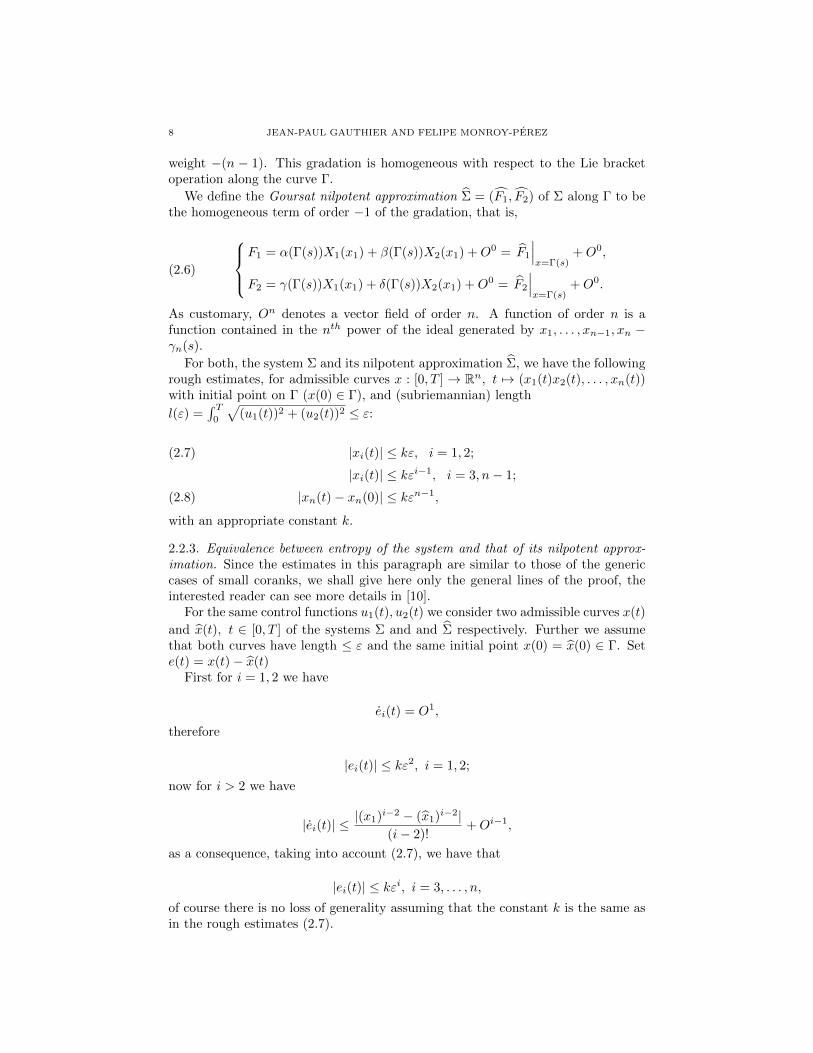
weight −(n − 1). This gradation is homogeneous with respect to the Lie bracketoperation along the curve Γ.

We define the Goursat nilpotent approximation Σ = (F1, F2) of Σ along Γ to bethe homogeneous term of order −1 of the gradation, that is,

(2.6)

F1 = α(Γ(s))X1(x1) + β(Γ(s))X2(x1) +O0 = F1

∣∣∣x=Γ(s)

+O0,

F2 = γ(Γ(s))X1(x1) + δ(Γ(s))X2(x1) +O0 = F2

∣∣∣x=Γ(s)

+O0.

As customary, On denotes a vector field of order n. A function of order n is afunction contained in the nth power of the ideal generated by x1, . . . , xn−1, xn −γn(s).

For both, the system Σ and its nilpotent approximation Σ, we have the followingrough estimates, for admissible curves x : [0, T ] → Rn, t 7→ (x1(t)x2(t), . . . , xn(t))with initial point on Γ (x(0) ∈ Γ), and (subriemannian) length

l(ε) =∫ T

0

√(u1(t))2 + (u2(t))2 ≤ ε:

|xi(t)| ≤ kε, i = 1, 2;(2.7)

|xi(t)| ≤ kεi−1, i = 3, n− 1;

|xn(t)− xn(0)| ≤ kεn−1,(2.8)

with an appropriate constant k.

2.2.3. Equivalence between entropy of the system and that of its nilpotent approx-imation. Since the estimates in this paragraph are similar to those of the genericcases of small coranks, we shall give here only the general lines of the proof, theinterested reader can see more details in [10].

For the same control functions u1(t), u2(t) we consider two admissible curves x(t)

and x(t), t ∈ [0, T ] of the systems Σ and and Σ respectively. Further we assumethat both curves have length ≤ ε and the same initial point x(0) = x(0) ∈ Γ. Sete(t) = x(t)− x(t)

First for i = 1, 2 we have

ei(t) = O1,

therefore

|ei(t)| ≤ kε2, i = 1, 2;

now for i > 2 we have

|ei(t)| ≤|(x1)i−2 − (x1)i−2|

(i− 2)!+Oi−1,

as a consequence, taking into account (2.7), we have that

|ei(t)| ≤ kεi, i = 3, . . . , n,

of course there is no loss of generality assuming that the constant k is the same asin the rough estimates (2.7).

MOTION PLANNING 9

This means that the subriemannian distance between x(t) and x(t) relative to

either Σ or Σ, is smaller than kε(1+ 1n−1 ), that is,

(2.9) d(x(t), x(t)) ≤ kε(1+ 1n−1 ).

With these estimates in hand, we can choose now a curve x(t) : [0, θ]→ Rn thatε−interpolates Γ by maximizing xn(θ), and applying the previous inequality to theinterpolating pieces, we get that

(2.10) EΣΓ (ε) ≤ EΣ

Γ (ε).

In this line of argumentation we can interchange the role of x and x to get finallythat:

(2.11) EΣΓ (ε) ≈ EΣ

Γ (ε)

2.3. Statement of the main result. Before stating the theorem, it is worthpointing out that our result can be understood and utilized in practical applicationsof motion planning, under two completely different viewpoints:

• One may think that the Goursat system is given, the car with trailers forinstance, and that it is put via feedback and change of coordinates underthe canonical form (2.3). After that, one chooses to apply the interpolationentropy strategy. This procedure shall provide an exact ε-interpolation con-trol strategy, but with a non-natural cost (due to the preliminary feedback).It is equivalent, after feedback, to solve the problem of finding admissible ε-interpolating curves that have an arbitrary but fixed subriemannian lengthgiven by (2.2), and that maximize the distance on Γ between two successiveinterpolated points. Under this strategy the actual size of ε is irrelevant.• The other viewpoint is to consider any subriemannian metric whatsoever

over the Goursat distribution, and to apply without preliminary feedback,the interpolation entropy strategy for small ε. In such a case, the metric isfree, but the result is asymptotic only (when ε → 0). It is noticeable thatthe (asymptotic) result is in fact independent of the chosen metric.

Our result is the following:

Theorem 2. (In Goursat coordinates, for model 2.6 or for its nilpotent approxi-

mation Σ.) A length one extremal of the interpolation problem between the originand a point of the xn axis, maximizing the endpoint coordinate xn can be explic-itly calculated. Its projection on the plane (x1, x2) is a closed hyperelliptic curve,smooth-periodic, with n − 2 loops, shown on figure 3 for n = 6, 7. The curve thatinterpolates with length ε is obtained from this one by homogeneity.

According to the estimates in paragraphs 2.2.2 and 2.2.3, what remains to bedone is to find the explicit equations for the extremals along with the correspondingprojections. The key point for proving this result is the fact that the Hamiltoniansystem of geodesic equations of the Goursat model is Liouville integrable whateverthe dimension n. We carry this out in the next section, following the integrationprocess developed in [16].


3. Extremal curves for the Goursat Case

3.1. The optimal control problem. As explained in the paragraph 2.1, in gen-eral the subriemannian geodesic problem on a subriemannian manifold is tanta-mount to an optimal control problem with quadratic cost. For our data G =(∆, g,Γ) we deal with a left invariant optimal control problem on the Goursat Liegroup G. This Lie group can be identified with Rn with the group law definedas follows, if g1 = (x1, . . . , xn) and g2 = (y1, . . . , yn) are two elements in G, theng1 ⊕ g2 = (z1, . . . , zn) with:

(3.1)

z1 = x1 + y1,

z2 = x2 + y2, and

zk = xk + yk +

k−1∑j=2

xk−j1

(k − j)!yj , for k = 3, . . . , n,

and the group identity e = (0, . . . , 0).The vector fields in the normal form (2.3) are ⊕−left invariant, and, as mentionedbefore, G is a simply connected n−step nilpotent Lie group with Lie algebra g,whose basis is defined by means of the commuting relations (2.4).

At the level of the nilpotent approximation of the left invariant control problemwe deal with is the following: among the admissible trajectories of the system

(3.2) g = u1(αX1(g) + βX2(g)) + u2(γX1(g) + δX2(g)), g ∈ G,

with αδ − βγ 6= 0, find the one that minimizes

(3.3)

∫(u1(t)2 + u2(t)2) dt.

As it is explained in the papers ( [8, 9, 10]), we have to find a minimizing geodesicof length 1 (homogeneity) connecting the origin to a point on the xn axis.

3.2. Gauge invariance of the metric. Any arbitrary nonsingular 2× 2 matrix

A =

(α γβ δ

),

can be written as A = TRϕ where Rϕ ∈ SO2 and T is a non-singular lower trian-gular 2× 2 matrix, say

T =

(a 0b c

), with ac 6= 0.

Since the rotation Rϕ preserves the metric it is enough to consider the constanttransformation given by T , in such a case the system (3.2) writes as follows

(3.4) g = (aX1(g) + bX2(g)) u1 + cX2(g) u2

and in coordinates we have

MOTION PLANNING 11

(3.5)

x1 = au1,

x2 = bu1 + cu2, and

xk = bxk−2

1

(k − 2)!u1 + c

xk−21

(k − 2)!u2, for k = 3, . . . , n.

We consider the change of coordinates

g = (x1, . . . , xn) 7→ g = (x1, . . . , xn),

given by

(3.6)

x1 =1

ax1,

x2 = − b

cax1 +

1

cx2, and

xk = − b

cak−1

xk−11

(k − 1)!+

1

cak−2xk for k = 3, . . . , n,

a straightforward computation yields

(3.7) ˙g = u1X2(g) + u2X2(g),

as can be easily verified.Furthermore the left invariance of the vector fields X1 and X2 implies that for

any h ∈ G we have

(3.8) 〈DLh( ˙g), DLh( ˙g)〉 = 〈 ˙g, ˙g〉 = u21 + u2

2,

where h 7→ Lh is the left translation.We summarize the result:

Theorem 3. Given a Goursat triple G = (∆, g,Γ), we can choose coordinatesalong Γ and orthonormal vector fields F1, F2 generating ∆, such that the nilpotentapproximation along Γ writes

x = X1(x)u1 +X2(x)u2,

and Γ(s) = (0, . . . , 0, ϕ(s)) for some smooth function ϕ(s).

Lemma 1. The map : G→ G, g 7→ g is an automorphism of G.

Proof. From the definition (3.6) it is clear that g 7→ g is a diffeomorphism. Letg1 = (x1, . . . , xn) and g2 = (y1, . . . , yn) be two arbitrary elements in G and letg1 ⊕ g2 = (z1, . . . zn). If we denote as g1 = (x1, . . . , xn), g2 = (y1, . . . , yn) and

g1 ⊕ g2 = (z1, . . . zn) the corresponding images, then the first two coordinates ofg1 ⊕ g2 are given by

x1 + y1 =1

ax1 +

1

ay1 = z1,

x2 + y2 =

(− b

cax1 +

1

cx2

)+

(− b

cay1 +

1

cy2

)= z2,


whereas for its kth coordinate, with k = 3, . . . , n we have

xk + yk +

k−1∑j=2

x k−j1

(k − j)!yj = − b

cak−1

xk−11

(k − 1)!+

1

cak−2xk

− b

cak−1

yk−11

(k − 1)!+

1

cak−2yk

+

k−1∑j=2

(x1

a

)k−j(k − j)!

[− b

caj−1

yj−11

(j − 1)!+

1

caj−2yj

]

= − b

cak−1

xk−11

(k − 1)!+

k−1∑j=2

xk−j1

(k − j)!yj−1

1

(j − 1)!+

yk−11

(k − 1)!

+

1

cak−2

xk + yk +

k−1∑j=2

xk−j1

(k − j)!yj

= − b

cak−1

(x1 + y1)k−1

(k − 1)!

+1

cak−2

xk + yk +

k−1∑j=2

xk−j1

(k − j)!yj

= zk.

It follows that g1 ⊕ g2 = g1 ⊕ g2

�

Now, a (weak) corollary of Theorem (3) and Lemma (1) is the following

Corollary 1. In the Goursat group, up to automorphisms, there is only one sub-riemannian left invariant metric that is defined by the normal form (2.3) with X1

and X2 orthonormal.

3.3. The entropy. Going back to the motion planning problem, we observe firstthat the automorphism (3.6) essentially does not change the reference path sincenow we have

s 7→ Γ(s) = (0, . . . , 0,1

can−2γn(s)),

and a formula for the entropy can be explicitly written.In fact, if ω is the 1−form that vanishes on the distribution ∆(n−2) and which

satisfies ω(Xn−1) = 1 where Xn−1 = [X1, Xn−2], then by denoting f(s) = ω(Γ(s))we have

(3.9) E(ε) ≈ E(ε) ≈∫

Γ

f(s) ds · An

εn

where An is a universal constant that depends on the dimension n only.

MOTION PLANNING 13

3.4. Application of the Pontryagin Maximum Principle. We now tackle theleft invariant optimal control problem on the Goursat group G consisting of theminimization of the functional

(3.10)

∫u2

1 + u22,

among the admissible trajectories of the left invariant control system

(3.11) g = u1X1(g) + u2X2(g),

with X1 and X2 given by the normal form (2.3) and satisfying the commutingrelations (2.4), the Lie algebra of G is denoted as g and can be identified with TeG.

As it is well known, Pontryagin maximum principle provides a standard geo-metric tool for the description of extremals by establishing necessary conditions foroptimality, for details we refer the reader to ( [20]).

If p denotes the dual variable in g∗, then for each vector field Xi we have the cor-responding Hamiltonian Hi = 〈p,Xi〉, i = 1, . . . n with Poisson brackets satisfyingcommuting relations dual to those of (2.4), that is,

(3.12) Hi = {H1, Hi−1}, i = 3, . . . n.

Maximality condition of the Pontryagin Maximum Principle yields

u1 = H1, and u2 = H2,

and the system Hamiltonian becomes quadratic

H =1

2(H2

1 +H22 ),

the associated adjoint equations are obtained by differentiating along the extremalas customary: Hi = {Hi,H}. In consequence, the commuting relations (3.12)clearly yield

H1 = H2H3(3.13)

H2 = −H1H3(3.14)

H3 = −H1H4(3.15)

...

Hi = −H1Hi+1(3.16)

...

Hn−3 = −H1Hn−2(3.17)

Hn−2 = −H1Hn−1(3.18)

Hn−1 = −H1Hn(3.19)

Hn = 0(3.20)

Therefore Hn is constant along extremals and shall be denoted


c1 := Hn = Hn(0).

3.5. Geometry of extremals. From equations (3.19) and (3.18) one gets

d

dt

(1

2!H2

n−1 − c1Hn−2

)= 0

Another conservation law is then obtained as

c2 :=1

2!H2

n−1(0)− c1Hn−2(0)

Now starting from the polynomial equation in the variables (Hn−1, Hn−2)

(3.21)1

2!H2

n−1 − c1Hn−2 − c2 = 0,

and using the adjoint system, a further conservation law can be generated by mul-tiplying for Hn−1:

1

2!H2

n−1Hn−1 − c1Hn−2Hn−1 − c2Hn−1 = 0,

for then equations (3.18) and (3.17) imply

d

dt

(1

3!H3

n−1 − c21Hn−3 − c2Hn−1

)= 0.

In consequence, another conservation law c3 is obtained and the procedure cancontinue with a polynomial equation in the variables (Hn−1, Hn−3)

1

3!H3

n−1 − c21Hn−3 − c2Hn−1 − c3 = 0.

Following this procedure of multiplying by Hn−1 and integrating, an extra con-servation law is obtained at each step j, together with a polynomial equation in thevariables (Hn−1, Hn−j) with j = 2, . . . , k. For instance, next step yields c4 togetherwith the polynomial equation in the variables (Hn−1, Hn−4)

1

4!H4

n−1 − c31Hn−4 −c22!H2

n−1 − c3Hn−1 − c4 = 0.

The last two steps of this process make use of equations (3.15) and (3.14) and(3.14) and (3.13) respectively. By performing the corresponding integration theconservation laws ck−1 and ck are obtained, together with the polynomial equationsin the variables (Hn−1, H3) and (Hn−1, H2)

1

(k − 1)!Hk−1

n−1 − ck−21 H3 −

k−1∑j=2

cj(k − 1− j)!

Hk−1−jn−1 = 0 and(3.22)

1

k!Hk

n−1 − ck−11 H2 −

k∑j=2

cj(k − j)!

Hk−jn−1 = 0,(3.23)

respectively. In conclusion we have the following

MOTION PLANNING 15

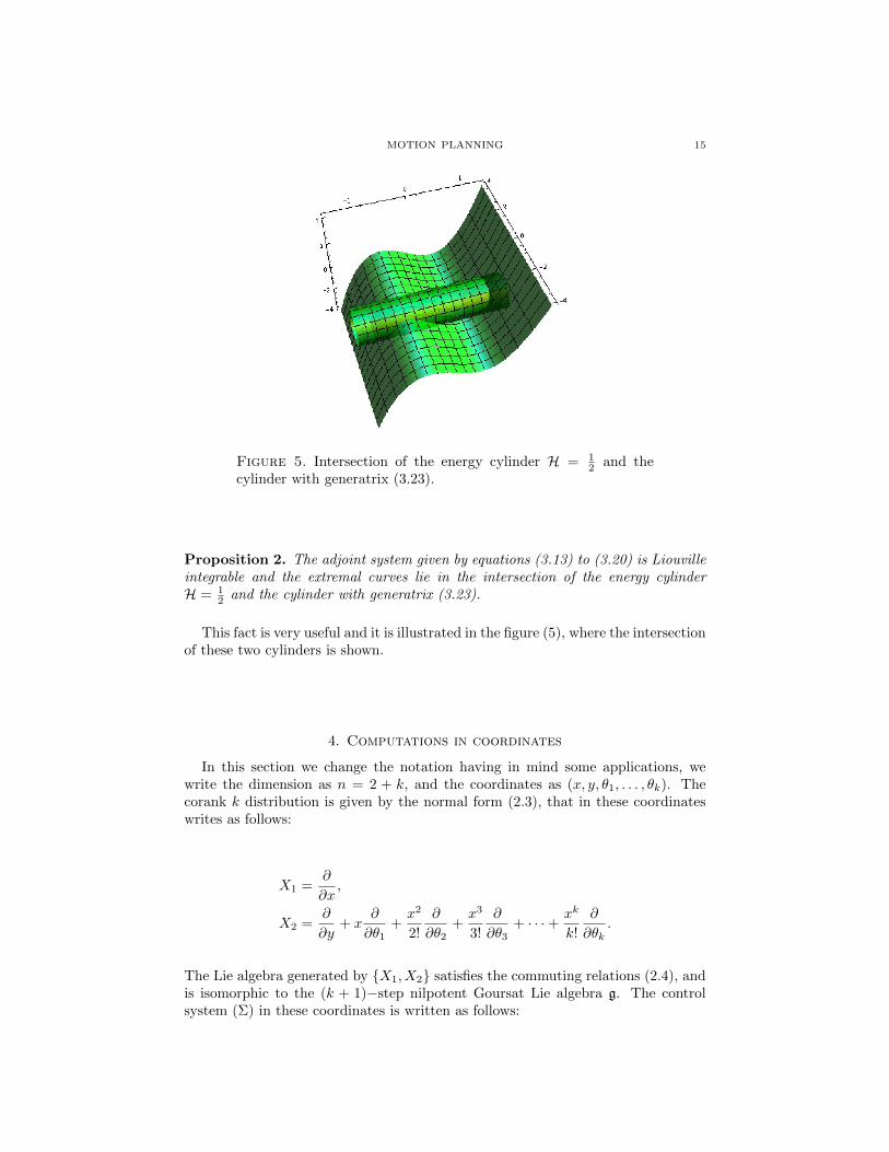
Figure 5. Intersection of the energy cylinder H = 12 and the

cylinder with generatrix (3.23).

Proposition 2. The adjoint system given by equations (3.13) to (3.20) is Liouvilleintegrable and the extremal curves lie in the intersection of the energy cylinderH = 1

2 and the cylinder with generatrix (3.23).

This fact is very useful and it is illustrated in the figure (5), where the intersectionof these two cylinders is shown.

4. Computations in coordinates

In this section we change the notation having in mind some applications, wewrite the dimension as n = 2 + k, and the coordinates as (x, y, θ1, . . . , θk). Thecorank k distribution is given by the normal form (2.3), that in these coordinateswrites as follows:

X1 =∂

∂x,

X2 =∂

∂y+ x

∂

∂θ1+x2

2!

∂

∂θ2+x3

3!

∂

∂θ3+ · · ·+ xk

k!

∂

∂θk.

The Lie algebra generated by {X1, X2} satisfies the commuting relations (2.4), andis isomorphic to the (k + 1)−step nilpotent Goursat Lie algebra g. The controlsystem (Σ) in these coordinates is written as follows:


x = u1

y = u2

θ1 = xu2

θ2 =x2

2!u2

θ3 =x3

3!u2

...

θk =xk

k!u2

The Pontryagin maximum principle applies in the same lines as before, to obtainthat along extremals one has

x = H1, y = H2 and θj = H2xj

j!

Lemma 2. Hn−1 is a linear function of x. Moreover x and y are periodic functionsof time.

Proof. In fact equation (3.19) writes

Hn−1 = −c1H1 = −c1x.In consequence:

Hn−1 = Hn−1(0)− c1(x− x(0)).

�

Without loss of generality we can assume that c1 = Hn = Hn(0) = −1 andHn−1(0) = x(0) = 0 in such a way that Hn−1 may be identified with x.

4.1. The hyperelliptic curve. Following the inductive procedure explained inparagraph (3.5) and assuming that c1 = −1 we can write equations (3.23) and(3.22) as follows:

H3 = − 1

(k − 1)!xk−1 +

k−1∑j=2

cj(k − 1− j)!

xk−1−j =: pk−1(x),(4.1)

H2 = − 1

k!xk +

k∑j=2

cj(k − j)!

xk−j =: pk(x).(4.2)

Here and in the remaining of the paper the subindex of a polynomial denote itsdegree. For then a further derivation of equation (3.19) together (3.13) yield

x = H1 = H2H3 = pk(x)pk−1(x) =: qk(k−1)(x),

and by multiplying both sides by x one gets

MOTION PLANNING 17

(x)2 = rk(k−1)+1(x).

As a consequence, x can be explicitly integrated by inverting the hyperellipticintegral

(4.3)

∫dx√

rk(k−1)+1(x)

4.2. Optimal curves. As projection of extremal curves, optimal solutions neces-sarily satisfy

x =√

1− p2k(x),(4.4)

y = pk(x), and(4.5)

θj =xj

j!pk(x), for j = 1, . . . k(4.6)

5. Motion planning for Goursat structures.

We use now the geometric information provided by the Pontryagin maximumprinciple and the hyperelliptic curve described above, for deriving the geometricfeatures that optimal trajectories in the plane {(x, y)} ' {(x, y, 0, . . . , 0)} necessar-ily have.

To begin with, we consider the three-dimensional space with coordinates

(x, u1, z) = (x, x, y) = (x, u1, u2) = (Hn−1, H1, H2),

and the following two cylinders:

C1 = {(x, u1, z) | u21 + z2 = 1} and C2 = {(x, u1, z) | z = pk(x)}.

We can assume that the C1 ∩ C2 6= ∅ and by choosing the initial conditionsproperly, we can assume that this intersection is a smooth, connected, closed andsimple curve. We denote by C the parametrized curve that is the projection ofC1 ∩ C2 to the plane {(x, u1)} ' {(x, u1, 0)}, and call it the cacahuete curve of theproblem, taking equation (4.4) into consideration we have:

C =

{(x, u1) | u1 =

√1− p2

k(x)

}.

The cacahuete is a smooth, closed and simple curve that has both, vertical andhorizontal symmetries, and by choosing the initial conditions properly it can beassumed that it is centered at the origin.

One can see on figure (5) how the cacahuete comes.The cacahuete encodes the information of extremal curves in the plane {(x, y)} '

{(x, y, 0, . . . , 0)} ⊂ {(x, y, θ1, . . . , θk)}. Let E be such an arc-length parametrizedextremal curve in this plane, taking equation (4.5) into account we have:

E = {(x, y) | y = pk(x)}.We assume E to be centered at the origin. Moreover, we want the curve E to havetotal length 1 (or ε), but this can be obtained a posteriori by homogeneity.


In order to depict the curve E we have the freedom of choosing the coefficientsof the polynomial pk(x) and the initial condition y(0). Also we have to take intoconsideration the following interpolation conditions (which are independent of anytranslation of coordinates):

(1) The coordinate y is periodic, y(1) = y(0).(2) The moments

mi =

∫Exidy

are all zero for i = 1, . . . , n−3, which corresponds to the fact that the coor-dinates θ1, . . . , θn−3, given by (4.5) are all periodic. Observe that the firstmoment m1 is the area swept out by the curve, whereas the last momentmn−2 is not only non vanishing but also the one to be maximized.

The curves E are symmetric with respect to the x-axis but we do not know ifthey are symmetric with respect to the y-axis, however we make this assumption,a priori reasonable.

Remark 5. • Since we will be able to find geodesics meeting this assumptionplus the boundary conditions, it is reasonable to expect that these geodesicsare optimal.• It is clear the union set of our centered solutions, is symmetric with respect

to the y-axis, but it is not clear that the minimal solution is unique.• Due to the interpolation requirements, it is clear that the projection of our

curve on the plane (x, y) has to be periodic. Moreover, with the grouplaw explicitly exhibited in (3.1) we can follow the same proof as in thepapers [8, 9], to show that this curve is in fact smooth-periodic.

Under these symmetry considerations and depending on the parity of n, (whichis the same parity of k) certain moments are automatically zero and the descriptionof E can always be completed.

• If n is even, the odd moments are zero. The polynomial pk(x) has evendegree and by the symmetry considerations, it has no terms of odd degree.Then, if we chose a monic polynomial, it remains k

2 free coefficients, that

have to be used to vanish k2 − 1 moments (plus the zero-moment y).

For instance, for n = 6, we have to chose only two coefficients tomake y periodic and to vanish the moment m2.

• if n is odd, the even moments are zero. The polynomial pk(x) has odddegree and by the symmetry considerations, it has no terms of even degree.Then, if we chose a monic polynomial, it remains k−1

2 free coefficients, that

have to be used to vanish k−12 moments and the value y(0) to make y

periodic, which can be done as an independent (trivial) step.For instance, for n = 7, we have to chose two coefficients to vanishtwo moments, and we chose the value y(0) to make y vanishingat a quarter period.

From this analysis we can conclude that, at the end we have as many free pa-rameters (plus one that accounts for the initial condition y(0)) as the number ofmoments that have to vanish.

MOTION PLANNING 19

Figure 6. Other periodic extremals for order 3 (length-4) brackets

In practice, we use the only following numerical integration:

dy

dx=

pk(x)√1− pk(x)2

,

and compute the solution for a quarter period only. The x corresponding to aquarter period (denoted by x 1

4) is just given by the largest real root of pk(x). The

value y(0) follows. Solutions over the other 3 intervals are obtained by symmetry.Hence, for both n = 6, 7, the computation reduces to this numerical integration

(over a quarter period), and to performing shooting on 2 coefficients of pk(x). Weobtained the numerical results that are presented in the introduction.

6. Conclusions and some open questions

In this paper we propose to use our entropy method of previous papers to treatthe motion-planning problem for Goursat sub-riemannian metrics in arbitrary di-mensions. We put in evidence a class of control trajectories and state trajectoriesthat are in a sense universal and optimal, and therefore we think that these signalsare the natural ones for dealing with motion planning questions. This conclusion isreinforced by the fact that it fits with the conclusions (in the generic cases, but forlow order brackets) of our previous studies.

In particular, our results apply to the motion planning of the car with trailers,which is the prototype of a Goursat structure. In this case, moreover, the methodcan be used in a direct way (not asymptotic) to interpolate non-admissible pathsby means of admissible ones.

In our view, there are many interesting issues to address in this regard, but wejust want to bring the attention to the following two challenging questions:

• Find arguments (like it was done in the paper [9]) to prove that our (sym-metric) Goursat extremals are actually optimal.• Prove (or find counterexample) that in the generic case the geometric

pattern of the pictures of optimal extremals persists, and depends only on


the length of the Lie brackets of the highest order. This is not so clear: whenthe order increases, the number of interpolation conditions increases muchmore (contrarily to what happens in the Goursat case), and it might happenthat some more complicated periodic extremals come into the picture. Someof these more complicated extremals were exhausted in [9]. We show one ofthem in the figure 6.

Aknowledgements

This paper was prepared during the sabbatical leave of the second author at theLaboratoire des Sciences de l’Information et des Systemes (LSIS, UMR 7296) in theUniversite du Sud Toulon-Var, France. The author was financially supported by theCONACYT under the program of sabbatical leaves abroad for the reinforcement ofthe research groups, project number 204051.

References

[1] H.J. Sussmann, and G. Laferriere, Motion planning for controllable systems without drift, InProceedings of the IEEE Conference on Robotics and Automation, Sacramento, CA, April

1991. IEEE Publications, NewYork, (1991), pp. 109-148.

[2] H.J. Sussmann, W.S. Liu, Lie bracket extensions and averaging: the single bracket generatingcase, Z. X. Li and J. F. Canny Eds., Kluwer Academic Publishers, Boston, (1993), pp. 109-

148.

[3] D. Tilbury, R.M. Murray, S. Sastry, Trajectory generation for the n-trailer problem usingGoursat normal form, IEEE Trans. Aut. Contr., Vol 40, No. 5, pp 802-819, 1995.

[4] D. Tilbury, J. Laumond, R. Murray, S. Sastry, and G. Walsh. Steering car-like systems withtrailers using sinusoids. In Proceedings of the IEEE International Conference on Robotics

and Automation (ICRA), pp. 1993–1998, 1992.

[5] F. Jean, Complexity of Nonholonomic Motion Planning, International Journal on Control,Vol74, N 8, (2001), pp. 776-782.

[6] F. Jean, Entropy and Complexity of a Path in subriemannian Geometry, COCV, Vol 9,

(2003), pp. 485-506.[7] F. Jean, E. Falbel, Measures and transverse paths in subriemannian geometry, Journal

d’Analyse Mathematique, Vol. 91, ( 2003), pp. 231- 246.

[8] N. Boizot, J.P. Gauthier, Motion Planning for Kinematic Systems, IEEE TAC, Vol 58, No.6, June 2013, pp. 1430-1442.

[9] N. Boizot, J.P. Gauthier, On the Motion Planning of the Ball with a Trailer, MathematicalControl and Related Fields, Vol. 3, No.3, pp. 269-286, 2013.

[10] J.P. Gauthier, V. Zakalyukin, On the motion planning problem, complexity, entropy and

nonholonomic interpolation, Journal of Dynamical and Control Systems, Vol 12, No.3, july

2006.[11] JP Gauthier, B. Jakubczyk, V. Zakalyukin, Motion planning and fastly oscillating controls,

SIAM Journ. On Control and Opt, Vol. 48 (5), pp. 3433-3448, 2010.[12] C. Romero-melendez, J.P. Gauthier, F. Monroy-Perez, On Complexity and Motion Planning

for Corank one Sub-riemannian Metrics, COCV, Vol 10, 2004, pp. 634-655.

[13] J.P. Gauthier, V. Zakalyukin, On the Codimension One Motion Planning Problem, Journalof Dynamical and Control Systems, Vol 11, No.1, pp 73-89, 2005.

[14] J.P. Gauthier, V. Zakalyukin; On the one-step-bracket-generating motion planning problem,

Jounal of dynamical and control systems, Vol 11 No. 2, pp.215-235, Avril 2005.[15] A. E. H. Love, A treatise on the mathematical theory of elasticity, Dover, New York (1944).

[16] A. Anzaldo-Meneses, F. Monroy-Perez, Goursat distributions and sub-riemannian structures,

Journal of Mathematical Physics, vol. 44, N12, 2003, pp.6101-6111.[17] J.P. Gauthier, M. Kawski, Minimal Complexity Sinusoidal Controls for Path Planning, sub-

mitted to CDC 2014, L.A., USA.

[18] A. Bellaiche, The Tangent Space in Sub-Riemannian geometry, Journal of MathematicalSciences, Vol 83 No.4, 1997.

MOTION PLANNING 21

[19] E. von Weber. Zur Invariantentheorie der Systeme Pfaff’scher Gleichungen.Berichte uber

die Verhandlungen der Koniglich Sachsischen Gesellshaft der Wissenshaften. Mathematisch-

Physikalische Klasse, Leipzig, 50:207–229, 1898.[20] A.A. Agrachev, Yu. L. Sachkov, A Control Theory from the Geometric Viewpoint, Springer;

(2004).

LSIS, UMR CNRS 7296 and Equipe INRIA GECO., Universite de Toulon, UTLN, 83957

La Garde CEDEX, FranceE-mail address: [email protected]

URL: http://www.lsis.org/jpg

Current address: Universidad Autonoma Metropolitana -Azcapotzalco, Mexico D.F., 02200,

Mexico

E-mail address: [email protected]

on certain hyperelliptic signals that are … · on certain hyperelliptic signals that are natural...

Documents