Inherent-Cost Aware Collective SpatialKeyword Queries

Chan, H. K-H., Long, C., & Wong, R. C-W. (2017). Inherent-Cost Aware Collective SpatialKeyword Queries. In2017 International Symposium on Spatial and Temporal Databases (SSTD 2017): Proceedings (Lecture Notesin Computer Science). Springer.

Published in:2017 International Symposium on Spatial and Temporal Databases (SSTD 2017): Proceedings

Document Version:Peer reviewed version

Queen's University Belfast - Research Portal:Link to publication record in Queen's University Belfast Research Portal

Publisher rights© 2017 Springer.This work is made available online in accordance with the publisher’s policies. Please refer to any applicable terms of use of the publisher.

General rightsCopyright for the publications made accessible via the Queen's University Belfast Research Portal is retained by the author(s) and / or othercopyright owners and it is a condition of accessing these publications that users recognise and abide by the legal requirements associatedwith these rights.

Take down policyThe Research Portal is Queen's institutional repository that provides access to Queen's research output. Every effort has been made toensure that content in the Research Portal does not infringe any person's rights, or applicable UK laws. If you discover content in theResearch Portal that you believe breaches copyright or violates any law, please contact openaccess@qub.ac.uk.

Download date:25. Aug. 2018

Inherent-Cost Aware Collective Spatial Keyword Queries

Harry Kai-Ho Chan1, Cheng Long2, and Raymond Chi-Wing Wong1

1 The Hong Kong University of Science and Technology{khchanak, raywong}@cse.ust.hk

2 Queen’s University Belfastcheng.long@qub.ac.uk

Abstract. With the proliferation of spatial-textual data such as location-basedservices and geo-tagged websites, spatial keyword queries become popular in theliterature. One example of these queries is the collective spatial keyword query(CoSKQ) which is to find a set of objects in the database such that it covers agiven set of query keywords collectively and has the smallest cost. Some exist-ing cost functions were proposed in the literature, which capture different aspectsof the distances among the objects in the set and the query. However, we observethat in some applications, each object has an inherent cost (e.g., workers havemonetary costs) which are not captured by any of the existing cost functions. Mo-tivated by this, in this paper, we propose a new cost function called the maximumdot size cost which captures both the distances among objects in a set and a queryas existing cost functions do and the inherent costs of the objects. We prove thatthe CoSKQ problem with the new cost function is NP-hard and develop two al-gorithms for the problem. One is an exact algorithm which is based on a novelsearch strategy and employs a few pruning techniques and the other is an approx-imate algorithm which provides a ln |q.ψ| approximation factor, where |q.ψ| de-notes the number of query keywords. We conducted extensive experiments basedon both real datasets and synthetic datasets, which verified our theoretical resultsand efficiency of our algorithms.

1 Introduction

Nowadays, geo-textual data which refers to data with both spatial and textual infor-mation is ubiquitous. Some examples of geo-textual data include the spatial points ofinterest with textual description, geo-tagged web objects (e.g., webpages and photosat Flicker), and also geo-social networking data (e.g., users of FourSquare have theircheck-in histories which are spatial and also profiles which are textual).

Collective Spatial Keyword Query (CoSKQ) [3,18,2] is a query type recently pro-posed on geo-textual data which is described as follows. LetO be a set of objects. Eachobject o ∈ O is associated with a spatial location, denoted by o.λ, and a set of key-words, denoted by o.ψ. Given a query q with a location q.λ and a set of keywords q.ψ,CoSKQ is to find a set S of objects such that S covers q.ψ, i.e., q.ψ ⊆ ∪o∈So.ψ, and thecost of S, denoted by cost(S), is minimized. CoSKQ is useful in applications wherea user wants to find a set of objects to collectively satisfy his/her needs. One exampleis that a tourist wants to find some points-of-interest to do sight-seeing, shopping anddining, where the user’s needs could be captured by the query keywords of a CoSKQ

query. Another example is that a manager wants to finds some workers, collectively of-fering a set of skills, to set up a project.

One key component of the CoSKQ problem is the cost function that measures thecost of a set of objects S wrt the query q, i.e., cost(S). In the literature, five differentcost functions have been proposed for cost(S) [3,18,2]. Each of these cost functions isbased on one or a few of the following distances: (D1) the sum of the distances betweenthe objects in S and q, (D2) the min of the distances between the objects in S and q,(D3) the max of the distances between the objects in S and q, and (D4) the max of thedistances between two objects in S. Specifically, (1) the sum cost function [3,2] definescost(S) as D1, (2) the maximum sum cost function [3,18,2] defines cost(S) as D3 +D4, (3) the diameter cost function [18] defines cost(S) as max{D1, D2}, (4) the summax cost function [2] defines cost(S) as D1 + D4, and (5) the min max cost function [2]defines cost(S) as D2 + D4.

These cost functions are suitable in applications where the cost of a set of objectscould be captured well by the spatial distances among the objects and the query only.For example, in the application where a tourist wants to find a set of points-of-interest,the cost is due to the distances to travel among the points-of-interest and the query.However, in some other applications, each object has an inherent cost and thus the costof a set of objects would be better captured by both the distances among the objectsand the query and the inherent costs of the objects. In the application where a managerwants to find a group of workers, each worker is associated with some monetary cost.Another example is that a tourist wants to visit some POIs (e.g, museums, parks), eachPOI is associated with an admission fee. Motivated by this, in this paper, we proposea new cost function called maximum dot size function which captures both some spa-tial distances between objects and a query and the inherent costs of the objects. Specif-ically, the maximum dot size function defines the cost of a set S of objects, denoted bycostMaxDotSize(S), as the multiplication between the maximum distance between theobjects in S and q and the sum of the inherent costs of objects in S.

The CoSKQ problem with the maximum dot size function is proven to be NP-hardand an exact algorithm would run in exponential time where the exponent is equal to thenumber of query keywords. We design an exact algorithm called MaxDotSize-E, whichadopts a novel strategy of traversing possible sets of objects so that only a small frac-tion of the search space is traversed (which is achieved by designing effective pruningtechniques which are made possible due to the search strategy). For better efficiency,we also design an approximate algorithm called MaxDotSize-A for the problem. Specif-ically, our main contribution is summarized as follows.

– Firstly, we propose a new cost function costMaxDotSize, which captures both thespatial distances between the objects and the query, and the inherent costs of theobjects.

– Secondly, we prove the NP-hardness of MaxDotSize-CoSKQ and design two algo-rithms, namely MaxDotSize-E and MaxDotSize-A. MaxDotSize-E is an exact algo-rithm and runs faster than an adapted algorithm in the literature [3]. MaxDotSize-Agives a solution set S with a ln |q.ψ|-factor approximation. In particular, if |S| ≤ 3it is guaranteed that S is an optimal solution.

– Thirdly, we conducted extensive experiments on both real and synthetic datasets,which verified our theoretical results and the efficiency of our algorithms.

The rest of this paper is organized as follows. Section 2 gives the related work. Sec-tion 3 defines the problem and discusses its hardness. Section 4 presents our proposedalgorithms. Section 5 gives the empirical study. Section 6 concludes the paper.

2 Related Work

Many existing studies on spatial keyword queries focus on retrieving a single objectthat is close to the query location and relevant to the query keywords.

A boolean kNN query [13,5,25,30] finds a list of k objects each covering all speci-fied query keywords. The objects in the list are ranked based on their spatial proximityto the query location.

A top-k kNN query [9,19,16,20,21,10,26] adopts the ranking function consideringboth the spatial proximity and the textual relevance of the objects and returns top-k ob-jects based on the ranking function. This type of queries has been studied on Euclideanspace [9,19,16], road network databases [20], trajectory databases [21,10] and movingobject databases [26]. Usually, the methods for this kind of queries adopt an index struc-ture called the IR-tree [9,24] capturing both the spatial proximity and the textual infor-mation of the objects to speed up the keyword-based nearest neighbor (NN) queries andrange queries. In this paper, we also adopt the IR-tree as an index structure.

Some other studies on spatial keyword queries focus on finding an object set asa solution. Among them, some [3,18,2] studied the collective spatial keyword queries(CoSKQ). These studies on CoSKQ adopted a few cost functions which capture thespatial distances among the objects and the query only and thus they are not suitable inapplications where objects are associated with inherent costs.

Another query that is similar to CoSKQ is the mCK query [28,29,15] which takes aset of m keywords as input and finds m objects with the minimum diameter that coverthe m keywords specified in the query. In the existing studies of mCK queries, it isusually assumed that each object contains a single keyword. There are some variants ofthe mCK query, including the SK-COVER [8] and the BKC query [11]. These queriesare similar to the CoSKQ problem in that they also return an object set that covers thequery keywords, but they only take a set of keywords as input.

There are also some other studies on spatial keyword queries, including [22] whichfinds top-k groups of objects with the ranking function considering the spatial proximityand textual relevance of the groups, [17] which takes a set of keywords and a clue asinputs, and returns k objects with highest similarities against the clue, [14,23] whichfinds an object set in the road network, [4,12] which finds a region as a solution and[1,27] which finds a route as a solution.

3 Problem Definition

Let O be a set of objects. Each object o ∈ O is associated with a location denoted byo.λ, a set of keywords denoted by o.ψ and an inherent cost denoted by o.cost. Given

two objects o and o′, we denote by d(o, o′) the Euclidean distance between o.λ and o′.λ.Given a query q which consists of a location q.λ and a set of keywords q.ψ, an object issaid to be relevant if it contains at least one keyword in q.ψ, and we denote by Oq theset containing all relevant objects and say a set of objects is feasible if it covers q.ψ.

Problem Definition [3]. Given a query q = (q.λ, q.ψ), the Collective Spatial KeywordQuery (CoSKQ) problem is to find a set S of objects in O such that S covers q.ψ andthe cost of S is minimized.

In this paper, we propose a new cost function called maximum dot size which definesthe cost of a set S of objects, denoted by costMaxDotSize(S), as the multiplication ofthe maximum distance between objects in S and q and the sum of the inherent costs ofobjects in S, i.e.,

costMaxDotSize(S) = maxo∈S

d(o, q) ·∑o∈S

o.cost (1)

For simplicity, we assume that each object has a unit cost and thus the overall inherentcost of a set of objects corresponds to the size of this set and costMaxDotSize(S) cor-responds to maxo∈S d(o, q) · |S|. However, the exact algorithm and the approximate al-gorithm developed in this paper could also be applied to the general case with arbitrarycosts, while all theoretical results (e.g., approximation ratio) remain applicable (detailscould be found in Section 4.4).

We define the maximum dot size function with distance D3 (i.e., maxo∈S d(o, q))because D3 is the distance traveled to the most far-away object, and it is able to cap-ture other distances (e.g., 2maxo∈S d(o, q) ≤ maxo1,o2∈S d(o1, o2)). We use a simpleproduct to combine the two factors (distance and inherent cost) such that it remains ap-plicable and meaningful when the object inherent costs are unavailable. Note that wediscarded the normalization term maxo∈O d(o, q) · |q.ψ| ·maxo∈O o.cost, which doesnot affect the applicability of the cost function.

The CoSKQ problem with the maximum dot size function is denoted asMaxDotSize-CoSKQ. In the following, if there is no ambiguity, we writecostMaxDotSize(·) as cost(·) for simplicity.

Intractability. The following lemma shows the NP-hardness of MaxDotSize-CoSKQ.

Lemma 1. MaxDotSize-CoSKQ is NP-hard.

Proof: We prove by transforming the set cover problem which is known to be NP-Complete to the MaxDotSize-CoSKQ problem. The description of the MaxDotSize-CoSKQ problem is given as follows. Given a set O of spatial objects, each o ∈ O isassociated with a location o.λ and a set of keywords o.ψ, a query q consisting of aquery location q.λ and a set of query keywords q.ψ, and a real number C, the problemis to determine whether there exists a set S of objects inO such that S covers the querykeywords and cost(S) is at most C.

The description of the set cover problem is given as follows. Given a universeset U = {e1, e2, ..., en} of n elements and a collection of m subsets of U , V ={V1, V2, ..., Vm}, and a number k, the problem is to determine whether there exists a setT ⊆ V such that T covers all the elements in U and |T | ≤ k.

We transform a set cover problem instance to a MaxDotSize-CoSKQ problem in-stance as follows. We construct a query q by setting q.λ to be an arbitrary location inthe space and q.ψ to be a set of n keywords each corresponding to an element in U . Weconstruct a set O such that O contains m objects each corresponding to a subset in V .For each object o in O, we set o.λ to be any location at the boundary of the disk whichis centered at q.λ and has the radius equal to 1, set o.ψ be a set of keywords correspond-ing to the elements in the subset in V that o is corresponding to and set o.cost = 1.Note that for any o ∈ O, we have d(o, q) = 1 and the MaxDotSize cost of any set ofobjects is exactly equal to the size of the set. Besides, we set C to be equal to k. Clearly,the above transformation can be done in polynomial time.

The equivalence between the set cover problem instance and the correspondingMaxDotSize-CoSKQ problem instance could be verified easily since if there exists aset T such that T cover all the elements in U and |T | ≤ k, the set of objects corre-sponding the subsets in T cover all the query keywords in q.ψ and has the MaxDotSizecost at most C and vice versa.

4 Algorithms for MaxDotSize-CoSKQ

4.1 An Exact Algorithm

In this section, we present our exact method called MaxDotSize-E for MaxDotSize-CoSKQ. Before we present the algorithm, we first introduce some notations. Givena query q and a non-negative real number r, we denote the circle or the disk cen-tered at q.λ with radius r by D(q, r). Given a feasible set S, the query distanceowner of S is defined to be the object o ∈ S that is most far away from q.λ (i.e.,o = argmaxo∈S d(o, q)). Given a query q and a keyword t, the t-keyword nearestneighbor of q, denoted by NN(q, t), is defined to be the nearest neighbor (NN) of qcontaining keyword t. Besides, we define the nearest neighbor set of q, denoted byN(q), to be the set containing q’s t-keyword nearest neighbor for each t ∈ q.ψ, i.e.,N(q) = ∪t∈q.ψNN(q, t). Note that N(q) is a feasible set.

The MaxDotSize-E algorithm is presented in Algorithm 1. At the beginning, it main-tains an object set S for storing the best-known solution found so far, which is initializedtoN(q). Then, it performs an iterative process where each iteration involves three steps.

1. Step 1 (Query Distance Owner Finding): It picks one relevant object o followingan ascending order of d(o, q).

2. Step 2 (Feasible Set Construction): It constructs the best feasible set S′ withobject o as the query distance owner via a procedure called “findBestFeasibleSet”.

3. Step 3 (Optimal Set Updating): It then updates S to S′ if cost(S′) < cost(S).

The iterative process continues with the next relevant object until all relevant objectshave been processed.

One remaining issue in Algorithm 1 is the “findBestFeasibleSet” procedure whichis shown in Algorithm 2.

First, it maintains a variable ψ, denoting the set of keywords in q.ψ not coveredby o yet, which is initialized as q.ψ − o.ψ. If ψ = ∅, then it returns {o} immedi-ately since we know that it is the best feasible set. Otherwise, it proceeds to retrieve the

Algorithm 1 Algorithm MaxDotSize-EInput: A query q and a set O of objectsOutput: A feasible set S with the smallest cost1: S ← N(q)2: // Step 1 (Query Distance Owner Finding)3: for each relevant object o in ascending order of d(o, q) do4: // Step 2 (Feasible Set Construction)5: S′ ← findBestFeasibleSet(o)6: // Step 3 (Optimal Set Updating)7: if S′ 6= ∅ and cost(S′) < cost(S) then8: S ← S′

9: return S

Algorithm 2 Algorithm for finding the best feasible set with object o as the querydistance owner (findBestFeasibleSet(o))Input: An object oOutput: The best feasible set with o as the query distance owner (if any)1: ψ ← q.ψ − o.ψ2: if ψ = ∅ then3: return {o}4: O′ ← a set of all relevant objects in D(q, d(o, q))5: if O′ does not cover ψ then6: return ∅7: for each subset S′′ ofO′ with size at most min{|ψ|, cost(S)

d(o,q)− 1} in ascending order of |S′′|

do8: if S′′ covers ψ then9: return S′′ ∪ {o}

10: return ∅

set O′ of all relevant objects in D(q, d(o, q)). If O′ does not cover ψ, it returns ∅ im-mediately. Otherwise, it enumerates each possible subset S′′ of O′ with size at mostmin{|ψ|, cost(S)d(o,q) − 1} in ascending order of |S′′| (by utilizing the inverted lists main-tained for each keyword in ψ), and checks whether S′′ covers ψ (note that |S′′| is atmost cost(S)d(o,q) − 1 because otherwise it cannot contribute to a better solution). If yes, itreturns S′′∪{o} immediately since it is the best feasible set inO′. Otherwise, it checksthe next subset of O′. When all subsets of O′ have been processed and there is no fea-sible set found, it returns ∅.

To further improve the efficiency of the MaxDotSize-E algorithm, we develop somepruning techniques in both Step 1 and Step 2.

4.1.1 Pruning in Step 1The major idea is that not each object o ∈ Oq is necessary to be considered as a querydistance owner of S′ to be constructed and thus some can be pruned. Specifically, wehave the following lemmas.

qdLB dUBo1 o6

o7

o4

o2o3

o5

Fig. 1. Distance constraint for query distance owners

Lemma 2 (Distance Constraint). Let So be the optimal set and o be the query distanceowner of So. Then, we have dLB ≤ d(o, q) ≤ dUB , where dLB = maxo∈N(q) d(o, q)and dUB = cost(S), where S is an arbitrary feasible set.

Proof: First, we prove dLB ≤ d(o, q) by contradiction. Assume d(o, q) < dLB . Letof be the farthest object from q in N(q), i.e., dLB = d(q, of ). There exists a keywordtf ∈ of .ψ ∩ q.ψ such that tf is not contained by any object that is closer to q than ofsince otherwise of 6∈ N(q). This leads to a contradiction since there exists an objecto′ ∈ So which covers tf and d(o′, q) ≤ d(o, q) < dLB .

Second, we prove d(o, q) ≤ dUB also by contradiction. Assume d(o, q) > dUB .Then cost(So) = d(o, q) · |So| > dUB · |So| > cost(S) which contradict the fact thatSo is the optimal set.

Figure 1 shows the distance constraint. We only need to consider the relevant objectsinside the gray area (i.e., o2, o3 and o5) to be the query distance owners.

Lemma 3 (Keyword Constraint). Let o be the query distance owner of the set S′ tobe constructed. If d(o, q) > dLB and |o.ψ ∩ q.ψ| < 2, there exist a feasible set S′′ s.t.cost(S′′) ≤ cost(S′).

Proof: Given the set S′, we can construct the feasible set S′′ as follows. Consider thefollowing two cases. Case 1. d(o, q) > dLB and |o.ψ ∩ q.ψ| = 0. In this case, we canconstruct S′′ = S′ \ {o} be the feasible set with lower cost. Case 2. d(o, q) > dLBand |o.ψ ∩ q.ψ| = 1. Let the keyword t = o.ψ ∩ q.ψ. We know that o 6∈ N(q) becaused(o, q) > dLB . Note that there exist an object o′ ∈ N(q) that contains t. Thus, we canconstruct S′′ = S′ \ {o} ∪ {o′} be the feasible set with cost(S′′) ≤ cost(S′).

The above two lemmas suggest that an object o could be pruned if any of the fol-lowing two conditions is not satisfied.

1. (Condition 1): dLB ≤ d(o, q) ≤ dUB ; and2. (Condition 2): (d(o, q) = dLB) or (d(o, q) > dLB and |o.ψ ∩ q.ψ| ≥ 2)

4.1.2 Pruning in Step 2The major idea is that not each object o′ ∈ O′ is necessary to be enumerated whenfinding the best feasible set S′ with the query distance owner o. We first introduce aconcept called dominance. Given a set of keywords ψ, a set of objects O′, two objectso1 and o2 inO′, we say that o1 dominates o2 wrt ψ if all keywords in ψ that are coveredby o2 can be covered by o1 and there exists a keyword in ψ that is covered by o1 but notby o2 (i.e., o2.ψ ∩ ψ ⊂ o1.ψ ∩ ψ). An object that is not dominated by another objectis said to be a dominant object. Then, it could be verified easily that only those objectsthat are dominant ones need to be considered in Step 2.

4.1.3 Correctness and Time ComplexityBased on the description of the MaxDotSize-E algorithm, it is easy to verify thatMaxDotSize-E is an exact algorithm.

Theorem 1. MaxDotSize-E returns a feasible set with the smallest cost forMaxDotSize-CoSKQ.

Time Complexity. We use the IR-tree built on O to support the range query operationsinvolved in the algorithm.

Let n1 be the number of iterations (lines 3-8) MaxDotSize-E and β be the cost ofexecuting one iteration. The time complexity of MaxDotSize-E isO(n1 ·β). In practice,we have n1 << |Oq| since n1 is equal to the number of relevant objects satisfying thetwo conditions.

Consider β. It is dominated by the cost of executing the “findBestFeasibleSet” pro-cedure with Algorithm 2 (line 5 of Algorithm 1). We analyze the cost of Algorithm 2as follows. The cost of lines 1-3 is dominated by that of the remaining parts in the al-gorithm. Line 4 could be finished by performing a range query with an additional con-straint that the object is relevant, which incurs the cost of O(log |O| + |O′|) [7]. Notethat |O′| corresponds to the number of objects returned by the range query. Lines 5-6 could be finished simply by traversing for each object in O′ the set of keywords as-sociated with it and thus the cost is O(

∑o∈O′ |o.ψ|). Lines 7-9 could be finished by

enumerating all possible subsets of O′ with size at most min{|ψ|, cost(S)d(o,q) − 1} in as-cending order of size and for each subset, checking whether it covers ψ, and thus thecost is bounded by O(|O′||ψ|

∑o∈O′ |o.ψ|) (since there are at most |O′||ψ| subsets to

be checked and the cost of checking each subset is bounded by∑o∈O′ |o.ψ|). Over-

all, we know that the time complexity of MaxDotSize-E is O(n1 · (log |O| + |O′| +∑o∈O′ |o.ψ|+|O′||ψ|

∑o∈O′ |o.ψ|)) = O(n1 ·(log |O|+|O′||ψ|

∑o∈O′ |o.ψ|)), where

we have n1 << |Oq|, |O′| ≤ |Oq|, and |ψ| < |q.ψ|.

4.2 An Approximate Algorithm

In this section, we introduce an approximate algorithm called MaxDotSize-A forMaxDotSize-CoSKQ, which gives a ln |q.ψ|-factor approximation.

MaxDotSize-A is exactly the same as the MaxDotSize-E except that it replaces the“findBestFeasibleSet” procedure which is an expensive exhaustive search process with

a greedy process which is much cheaper. Specifically, the greedy process first initial-izes the set to be returned to {o} and then iteratively selects an object in the diskD(q, d(o, q)) which has the greatest number of uncovered keywords and inserts it intothe set until all keywords are covered.

Theoretical Analysis. Although the set S returned by the MaxDotSize-A algorithmmight have a larger cost than the optimal set So, the difference is bounded.

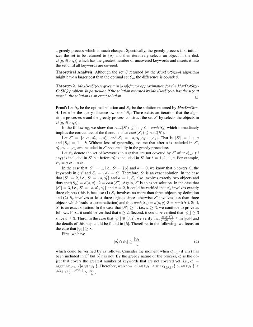
Theorem 2. MaxDotSize-A gives a ln |q.ψ|-factor approximation for the MaxDotSize-CoSKQ problem. In particular, if the solution returned by MaxDotSize-A has the size atmost 3, the solution is an exact solution.

Proof: Let So be the optimal solution and Sa be the solution returned by MaxDotSize-A. Let o be the query distance owner of So. There exists an iteration that the algo-rithm processes o and the greedy process construct the set S′ by selects the objects inD(q, d(o, q)).

In the following, we show that cost(S′) ≤ ln |q.ψ| · cost(So) which immediatelyimplies the correctness of the theorem since cost(Sa) ≤ cost(S′).

Let S′ = {o, o′1, o′2, ..., o′a} and So = {o, o1, o2, ..., ob}. That is, |S′| = 1 + aand |So| = 1 + b. Without loss of generality, assume that after o is included in S′,o′1, o

′2, ..., o

′a are included in S′ sequentially in the greedy procedure.

Let ψt denote the set of keywords in q.ψ that are not covered by S′ after o′t−1 (ifany) is included in S′ but before o′t is included in S′ for t = 1, 2, ..., a. For example,ψ1 = q.ψ − o.ψ.

In the case that |S′| = 1, i.e., S′ = {o} and a = 0, we know that o covers all thekeywords in q.ψ and So = {o} = S′. Therefore, S′ is an exact solution. In the casethat |S′| = 2, i.e., S′ = {o, o′1} and a = 1, So also involves exactly two objects andthus cost(So) = d(o, q) · 2 = cost(S′). Again, S′ is an exact solution. In the case that|S′| = 3, i.e., S′ = {o, o′1, o′2} and a = 2, it could be verified that So involves exactlythree objects (this is because (1) So involves no more than three objects by definitionand (2) So involves at least three objects since otherwise S′ involves less than threeobjects which leads to a contradiction) and thus cost(So) = d(o, q)·3 = cost(S′). Still,S′ is an exact solution. In the case that |S′| ≥ 4, i.e., a ≥ 3, we continue to prove asfollows. First, it could be verified that b ≥ 2. Second, it could be verified that |ψ1| ≥ 3

since a ≥ 3. Third, in the case that |ψ1| ∈ [3, 7], we verify that cost(S′)

cost(So)≤ ln |q.ψ| and

the details of this step could be found in [6]. Therefore, in the following, we focus onthe case that |ψ1| ≥ 8.

First, we have

|o′t ∩ ψt| ≥|ψt|b

(2)

which could be verified by as follows. Consider the moment when o′t−1 (if any) hasbeen included in S′ but o′t has not. By the greedy nature of the process, o′t is the ob-ject that covers the greatest number of keywords that are not covered yet, i.e., o′t =argmaxo∈O′{|o.ψ∩ψt|}. Therefore, we know |o′t.ψ∩ψt| ≥ max1≤i≤b{|oi.ψ∩ψt|} ≥∑

1≤i≤b |oi.ψ∩ψt|b ≥ |ψt|

b .

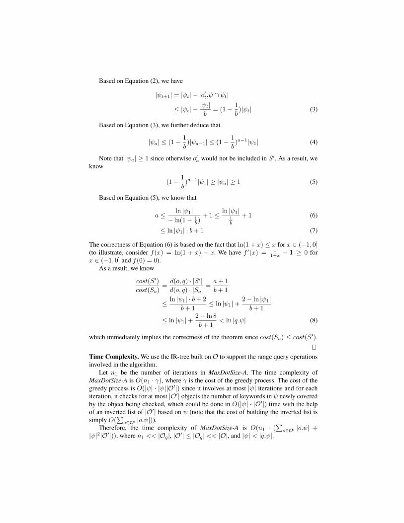
Based on Equation (2), we have

|ψt+1| = |ψt| − |o′t.ψ ∩ ψt|

≤ |ψt| −|ψt|b

= (1− 1

b)|ψt| (3)

Based on Equation (3), we further deduce that

|ψa| ≤ (1− 1

b)|ψa−1| ≤ (1− 1

b)a−1|ψ1| (4)

Note that |ψa| ≥ 1 since otherwise o′a would not be included in S′. As a result, weknow

(1− 1

b)a−1|ψ1| ≥ |ψa| ≥ 1 (5)

Based on Equation (5), we know that

a ≤ ln |ψ1|− ln(1− 1

b )+ 1 ≤ ln |ψ1|

1b

+ 1 (6)

≤ ln |ψ1| · b+ 1 (7)

The correctness of Equation (6) is based on the fact that ln(1 + x) ≤ x for x ∈ (−1, 0](to illustrate, consider f(x) = ln(1 + x) − x. We have f ′(x) = 1

1+x − 1 ≥ 0 forx ∈ (−1, 0] and f(0) = 0).

As a result, we know

cost(S′)

cost(So)=d(o, q) · |S′|d(o, q) · |So|

=a+ 1

b+ 1

≤ ln |ψ1| · b+ 2

b+ 1≤ ln |ψ1|+

2− ln |ψ1|b+ 1

≤ ln |ψ1|+2− ln 8

b+ 1< ln |q.ψ| (8)

which immediately implies the correctness of the theorem since cost(Sa) ≤ cost(S′).

Time Complexity. We use the IR-tree built on O to support the range query operationsinvolved in the algorithm.

Let n1 be the number of iterations in MaxDotSize-A. The time complexity ofMaxDotSize-A is O(n1 · γ), where γ is the cost of the greedy process. The cost of thegreedy process is O(|ψ| · |ψ||O′|) since it involves at most |ψ| iterations and for eachiteration, it checks for at most |O′| objects the number of keywords in ψ newly coveredby the object being checked, which could be done in O(|ψ| · |O′|) time with the helpof an inverted list of |O′| based on ψ (note that the cost of building the inverted list issimply O(

∑o∈O′ |o.ψ|)).

Therefore, the time complexity of MaxDotSize-A is O(n1 · (∑o∈O′ |o.ψ| +

|ψ|2|O′|)), where n1 << |Oq|, |O′| ≤ |Oq| << |O|, and |ψ| < |q.ψ|.

4.3 Adaptations of Existing Algorithms

In this section, we adapt the existing algorithms in [3,18,2], which are originally de-signed for CoSKQ problem with other cost functions, for MaxDotSize-CoSKQ.

Cao-E. Cao-E is an exact algorithm proposed in [3] for CoSKQ problem withcostMaxSum. It can be adapted to MaxDotSize-CoSKQ problem directly by replacingthe cost function from costMaxSum to costMaxDotSize, because it is a best-first searchalgorithm which is independent of the cost function used in the problem.

Other Exact Algorithms. Some other exact algorithms were proposed in the litera-ture for CoSKQ problem with different cost functions, namely Cao-Sum-E [3,2] (forcostSum), Cao-E-New [2] (for either costMaxSum or costMinMax) and Long-E [18](for either costMaxSum or costDia). They cannot be adapted to CoSKQ problem withcostMaxDotSize because they all rely on the property of their original cost functions.Consider Long-E as an example. The core of Long-E relies on an important propertyof the distance owner group (containing three objects) that different sets of objectswith the same distance owner group have the same cost for the cost function of eithercostMaxSum or costDia studied in [18]. However, this important property could not beapplied to our cost function studied in this paper, i.e., costMaxDotSize. In fact, it is pos-sible that two sets of objects with the same distance owner group have different costsfor the cost function of costMaxDotSize.

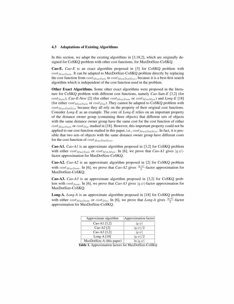
Cao-A1. Cao-A1 is an approximate algorithm proposed in [3,2] for CoSKQ problemwith either costMaxSum or costMinMax. In [6], we prove that Cao-A1 gives |q.ψ|-factor approximation for MaxDotSize-CoSKQ.

Cao-A2. Cao-A2 is an approximate algorithm proposed in [2] for CoSKQ problemwith costMaxSum. In [6], we prove that Cao-A2 gives |q.ψ|2 -factor approximation forMaxDotSize-CoSKQ.

Cao-A3. Cao-A3 is an approximate algorithm proposed in [3,2] for CoSKQ prob-lem with costSum. In [6], we prove that Cao-A3 gives |q.ψ|-factor approximation forMaxDotSize-CoSKQ.

Long-A. Long-A is an approximate algorithm proposed in [18] for CoSKQ problemwith either costMaxSum or costDia. In [6], we prove that Long-A gives |q.ψ|2 -factorapproximation for MaxDotSize-CoSKQ.

Approximate algorithm Approximation factorCao-A1 [3,2] |q.ψ|Cao-A2 [2] |q.ψ|/2

Cao-A3 [3,2] |q.ψ|Long-A [18] |q.ψ|/2

MaxDotSize-A (this paper) ln |q.ψ|Table 1. Approximation factors for MaxDotSize-CoSKQ

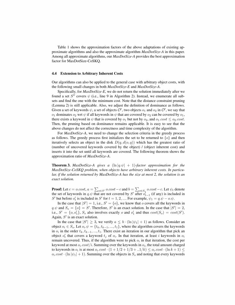
Table 1 shows the approximation factors of the above adaptations of existing ap-proximate algorithms and also the approximate algorithm MaxDotSize-A in this paper.Among all approximate algorithms, our MaxDotSize-A provides the best approximationfactor for MaxDotSize-CoSKQ.

4.4 Extension to Arbitrary Inherent Costs

Our algorithms can also be applied to the general case with arbitrary object costs, withthe following small changes in both MaxDotSize-E and MaxDotSize-A.

Specifically, for MaxDotSize-E, we do not return the solution immediately after wefound a set S′′ covers ψ (i.e., line 9 in Algorithm 2). Instead, we enumerate all sub-sets and find the one with the minimum cost. Note that the distance constraint pruning(Lemma 2) is still applicable. Also, we adjust the definition of dominance as follows.Given a set of keywords ψ, a set of objects O′, two objects o1 and o2 in O′, we say thato1 dominates o2 wrt ψ if all keywords in ψ that are covered by o2 can be covered by o1,there exists a keyword in ψ that is covered by o1 but not by o2, and o1.cost ≤ o2.cost.Then, the pruning based on dominance remains applicable. It is easy to see that theabove changes do not affect the correctness and time complexity of the algorithm.

For MaxDotSize-A, we need to change the selection criteria in the greedy processas follows. The greedy process first initializes the set to be returned to {o} and theniteratively selects an object in the disk D(q, d(o, q)) which has the greatest ratio of(number of uncovered keywords covered by the object) / (object inherent cost) andinserts it into the set until all keywords are covered. The following theorem shows theapproximation ratio of MaxDotSize-A.

Theorem 3. MaxDotSize-A gives a (ln |q.ψ| + 1)-factor approximation for theMaxDotSize-CoSKQ problem, when objects have arbitrary inherent costs. In particu-lar, if the solution returned by MaxDotSize-A has the size at most 2, the solution is anexact solution.

Proof: Let c = o.cost, a =∑o∈S′ o.cost−c and b =

∑o∈So

o.cost−c. Let ψt denotethe set of keywords in q.ψ that are not covered by S′ after o′t−1 (if any) is included inS′ but before o′t is included in S′ for t = 1, 2, .... For example, ψ1 = q.ψ − o.ψ.

In the case that |S′| = 1, i.e., S′ = {o}, we know that o covers all the keywords inq.ψ and So = {o} = S′. Therefore, S′ is an exact solution. In the case that |S′| = 2,i.e., S′ = {o, o′1}, So also involves exactly o and o′1 and thus cost(So) = cost(S′).Again, S′ is an exact solution.

In the case that |S′| ≥ 3, we verify a ≤ b · (ln |ψ1| + 1) as follows. Consider anobject oi ∈ So. Let oi.ψ = {tk, tk−1, ..., t1}, where the algorithm covers the keywordsin oi in the order tk, tk−1, ..., t1. There exist an iteration in our algorithm that pick anobject o′t that covers a keyword tj of oi. In that iteration, at least i keywords in oiremain uncovered. Thus, if the algorithm were to pick oi in that iteration, the cost perkeyword at most oi.cost/i. Summing over the keywords in oi, the total amount chargedto keywords in oi is at most oi.cost · (1 + 1/2 + 1/3 + ..1/k) ≤ oi.cost · (ln k + 1) ≤oi.cost · (ln |ψ1|+ 1). Summing over the objects in So and noting that every keywords

in ψ1 is covered by some objects in So, we get

a =∑

oi∈So\o

oi.cost · (ln |ψ1|+ 1)

= b · (ln |ψ1|+ 1) (9)

Therefore, we know

cost(S′)

cost(So)=d(o, q) ·

∑o∈S′ o.cost

d(o, q) ·∑o∈So

o.cost=a+ c

b+ c

≤ b · (ln |ψ1|+ 1) + c

b+ c

≤ ln |ψ1|+ 1− c · (ln |ψ1|+ 1)

b+ c< ln |q.ψ|+ 1 (10)

which immediately implies the correctness of the theorem since cost(Sa) ≤ cost(S′).

It is easy to see that changing the object selection criteria does not affect the timecomplexity of the algorithm.

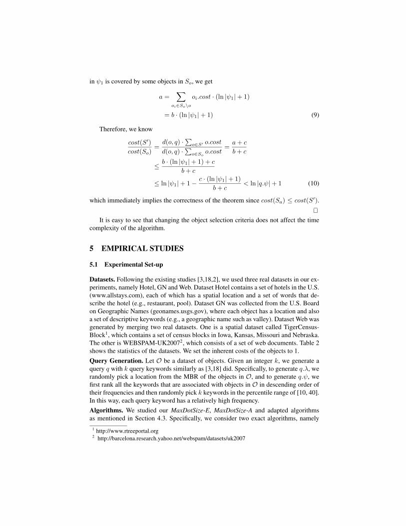
5 EMPIRICAL STUDIES

5.1 Experimental Set-up

Datasets. Following the existing studies [3,18,2], we used three real datasets in our ex-periments, namely Hotel, GN and Web. Dataset Hotel contains a set of hotels in the U.S.(www.allstays.com), each of which has a spatial location and a set of words that de-scribe the hotel (e.g., restaurant, pool). Dataset GN was collected from the U.S. Boardon Geographic Names (geonames.usgs.gov), where each object has a location and alsoa set of descriptive keywords (e.g., a geographic name such as valley). Dataset Web wasgenerated by merging two real datasets. One is a spatial dataset called TigerCensus-Block1, which contains a set of census blocks in Iowa, Kansas, Missouri and Nebraska.The other is WEBSPAM-UK20072, which consists of a set of web documents. Table 2shows the statistics of the datasets. We set the inherent costs of the objects to 1.Query Generation. Let O be a dataset of objects. Given an integer k, we generate aquery q with k query keywords similarly as [3,18] did. Specifically, to generate q.λ, werandomly pick a location from the MBR of the objects in O, and to generate q.ψ, wefirst rank all the keywords that are associated with objects in O in descending order oftheir frequencies and then randomly pick k keywords in the percentile range of [10, 40].In this way, each query keyword has a relatively high frequency.Algorithms. We studied our MaxDotSize-E, MaxDotSize-A and adapted algorithmsas mentioned in Section 4.3. Specifically, we consider two exact algorithms, namely

1 http://www.rtreeportal.org2 http://barcelona.research.yahoo.net/webspam/datasets/uk2007

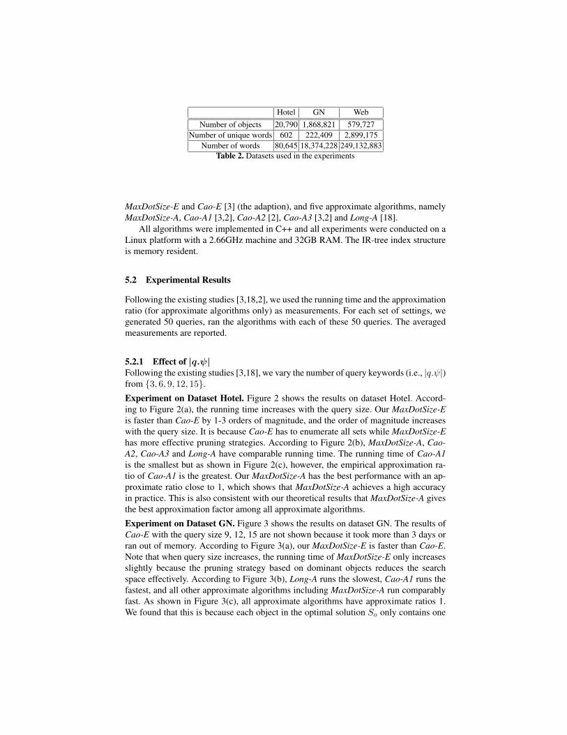
Hotel GN WebNumber of objects 20,790 1,868,821 579,727

Number of unique words 602 222,409 2,899,175Number of words 80,645 18,374,228 249,132,883

Table 2. Datasets used in the experiments

MaxDotSize-E and Cao-E [3] (the adaption), and five approximate algorithms, namelyMaxDotSize-A, Cao-A1 [3,2], Cao-A2 [2], Cao-A3 [3,2] and Long-A [18].

All algorithms were implemented in C++ and all experiments were conducted on aLinux platform with a 2.66GHz machine and 32GB RAM. The IR-tree index structureis memory resident.

5.2 Experimental Results

Following the existing studies [3,18,2], we used the running time and the approximationratio (for approximate algorithms only) as measurements. For each set of settings, wegenerated 50 queries, ran the algorithms with each of these 50 queries. The averagedmeasurements are reported.

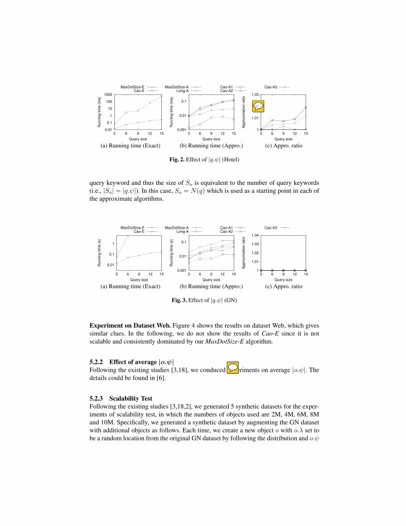
5.2.1 Effect of |q.ψ|Following the existing studies [3,18], we vary the number of query keywords (i.e., |q.ψ|)from {3, 6, 9, 12, 15}.Experiment on Dataset Hotel. Figure 2 shows the results on dataset Hotel. Accord-ing to Figure 2(a), the running time increases with the query size. Our MaxDotSize-Eis faster than Cao-E by 1-3 orders of magnitude, and the order of magnitude increaseswith the query size. It is because Cao-E has to enumerate all sets while MaxDotSize-Ehas more effective pruning strategies. According to Figure 2(b), MaxDotSize-A, Cao-A2, Cao-A3 and Long-A have comparable running time. The running time of Cao-A1is the smallest but as shown in Figure 2(c), however, the empirical approximation ra-tio of Cao-A1 is the greatest. Our MaxDotSize-A has the best performance with an ap-proximate ratio close to 1, which shows that MaxDotSize-A achieves a high accuracyin practice. This is also consistent with our theoretical results that MaxDotSize-A givesthe best approximation factor among all approximate algorithms.

Experiment on Dataset GN. Figure 3 shows the results on dataset GN. The results ofCao-E with the query size 9, 12, 15 are not shown because it took more than 3 days orran out of memory. According to Figure 3(a), our MaxDotSize-E is faster than Cao-E.Note that when query size increases, the running time of MaxDotSize-E only increasesslightly because the pruning strategy based on dominant objects reduces the searchspace effectively. According to Figure 3(b), Long-A runs the slowest, Cao-A1 runs thefastest, and all other approximate algorithms including MaxDotSize-A run comparablyfast. As shown in Figure 3(c), all approximate algorithms have approximate ratios 1.We found that this is because each object in the optimal solution So only contains one

MaxDotSize-ECao-E

MaxDotSize-A Long-A

Cao-A1 Cao-A2

Cao-A3

0.01

0.1

1

10

100

1000

3 6 9 12 15

Runnin

g tim

e (

ms)

Query size

0.001

0.01

0.1

3 6 9 12 15

Runnin

g tim

e (

ms)

Query size

1

1.01

1.02

1.03

3 6 9 12 15

Appro

xim

ation r

atio

Query size

(a) Running time (Exact) (b) Running time (Appro.) (c) Appro. ratio

Fig. 2. Effect of |q.ψ| (Hotel)

query keyword and thus the size of So is equivalent to the number of query keywords(i.e., |So| = |q.ψ|). In this case, So = N(q) which is used as a starting point in each ofthe approximate algorithms.

MaxDotSize-ECao-E

MaxDotSize-A Long-A

Cao-A1 Cao-A2

Cao-A3

0.01

0.1

1

3 6 9 12 15

Runnin

g tim

e (

s)

Query size

0.001

0.01

0.1

3 6 9 12 15

Runnin

g tim

e (

s)

Query size

1

1.01

1.02

1.03

1.04

3 6 9 12 15

Appro

xim

ation r

atio

Query size

(a) Running time (Exact) (b) Running time (Appro.) (c) Appro. ratio

Fig. 3. Effect of |q.ψ| (GN)

Experiment on Dataset Web. Figure 4 shows the results on dataset Web, which givessimilar clues. In the following, we do not show the results of Cao-E since it is notscalable and consistently dominated by our MaxDotSize-E algorithm.

5.2.2 Effect of average |o.ψ|Following the existing studies [3,18], we conduced experiments on average |o.ψ|. Thedetails could be found in [6].

5.2.3 Scalability TestFollowing the existing studies [3,18,2], we generated 5 synthetic datasets for the exper-iments of scalability test, in which the numbers of objects used are 2M, 4M, 6M, 8Mand 10M. Specifically, we generated a synthetic dataset by augmenting the GN datasetwith additional objects as follows. Each time, we create a new object o with o.λ set tobe a random location from the original GN dataset by following the distribution and o.ψ

MaxDotSize-ECao-E

MaxDotSize-A Long-A

Cao-A1 Cao-A2

Cao-A3

0.1

1

10

100

1000

3 6 9 12 15

Runnin

g tim

e (

s)

Query size

0.01

0.1

1

3 6 9 12 15

Runnin

g tim

e (

s)

Query size

1

1.001

1.002

1.003

3 6 9 12 15

Appro

xim

ation r

atio

Query size

(a) Running time (Exact) (b) Running time (Appro.) (c) Appro. ratio

Fig. 4. Effect of |q.ψ| (Web)

set to be a random document from GN and then add it into the GN dataset. We vary thenumber of objects from {2M, 4M, 6M, 8M, 10M}, and the query size |q.ψ| is set to 6.

Figures 5 shows the results for the scalability test. According to Figure 5(a), ourMaxDotSize-E is scalable wrt the number of objects in the datasets, e.g., it ran within10 seconds on a dataset with 10M objects. Besides, according to Figure 5(b), ourMaxDotSize-A runs consistently faster than Cao-A2 and Long-A and it is scalable, e.g.,it ran within 1 second on a dataset with 10M objects. According to Figure 5(c), all ap-proximate algorithms can achieve approximation ratios close to 1.

MaxDotSize-EMaxDotSize-A

Long-A Cao-A1

Cao-A2 Cao-A3

0.1

1

10

2M 4M 6M 8M 10M

Runnin

g tim

e (

s)

Number of objects

0.01

0.1

1

10

2M 4M 6M 8M 10M

Runnin

g tim

e (

s)

Number of objects

1

1.01

1.02

1.03

1.04

2M 4M 6M 8M 10M

Appro

xim

ation r

atio

Number of objects

(a) Running time (Exact) (b) Running time (Appro.) (c) Appro. ratio

Fig. 5. Scalability test

5.2.4 Objects with Inherent CostWe further generated a dataset based on the Hotel dataset, where each object is asso-ciated with an inherent cost. For each object, we assign an integer inherent cost in therange [1, 5] randomly.

Figure 6 shows the results. As shown in Figure 6(a) and (b), the running time of thealgorithms are similar to the case without object inherent cost (i.e., Figure 2(a) and (b)).According to Figure 6(c), the approximation ratio of our MaxDotSize-A is near to 1,which shows that the accuracy of MaxDotSize-A is high in practice. The approximationratio showed in the figure corresponds to the average of 50 queries, we found that the

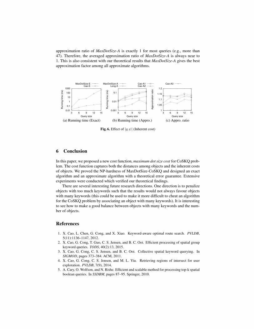
approximation ratio of MaxDotSize-A is exactly 1 for most queries (e.g., more than47). Therefore, the averaged approximation ratio of MaxDotSize-A is always near to1. This is also consistent with our theoretical results that MaxDotSize-A gives the bestapproximation factor among all approximate algorithms.

MaxDotSize-ECao-E

MaxDotSize-A Long-A

Cao-A1 Cao-A2

Cao-A3

0.01

0.1

1

10

100

1000

3 6 9 12 15

Runnin

g tim

e (

ms)

Query size

0.001

0.01

0.1

3 6 9 12 15

Runnin

g tim

e (

ms)

Query size

1

1.05

1.1

1.15

1.2

3 6 9 12 15

Appro

xim

ation r

atio

Query size

(a) Running time (Exact) (b) Running time (Appro.) (c) Appro. ratio

Fig. 6. Effect of |q.ψ| (Inherent cost)

6 Conclusion

In this paper, we proposed a new cost function, maximum dot size cost for CoSKQ prob-lem. The cost function captures both the distances among objects and the inherent costsof objects. We proved the NP-hardness of MaxDotSize-CoSKQ and designed an exactalgorithm and an approximate algorithm with a theoretical error guarantee. Extensiveexperiments were conducted which verified our theoretical findings.

There are several interesting future research directions. One direction is to penalizeobjects with too much keywords such that the results would not always favour objectswith many keywords (this could be used to make it more difficult to cheat an algorithmfor the CoSKQ problem by associating an object with many keywords). It is interestingto see how to make a good balance between objects with many keywords and the num-ber of objects.

References

1. X. Cao, L. Chen, G. Cong, and X. Xiao. Keyword-aware optimal route search. PVLDB,5(11):1136–1147, 2012.

2. X. Cao, G. Cong, T. Guo, C. S. Jensen, and B. C. Ooi. Efficient processing of spatial groupkeyword queries. TODS, 40(2):13, 2015.

3. X. Cao, G. Cong, C. S. Jensen, and B. C. Ooi. Collective spatial keyword querying. InSIGMOD, pages 373–384. ACM, 2011.

4. X. Cao, G. Cong, C. S. Jensen, and M. L. Yiu. Retrieving regions of intersect for userexploration. PVLDB, 7(9), 2014.

5. A. Cary, O. Wolfson, and N. Rishe. Efficient and scalable method for processing top-k spatialboolean queries. In SSDBM, pages 87–95. Springer, 2010.

6. H. K.-H. Chan, C. Long, and R. C.-W. Wong. Inherent-cost aware collective spatial key-word queries (full version). In http://www.cse.ust.hk/˜khchanak/paper/sstd17-coskq-full.pdf, 2017.

7. B. Chazelle, R. Cole, F. P. Preparata, and C. Yap. New upper bounds for neighbor searching.Information and control, 68(1):105–124, 1986.

8. D.-W. Choi, J. Pei, and X. Lin. Finding the minimum spatial keyword cover. In ICDE, pages685–696. IEEE, 2016.

9. G. Cong, C. S. Jensen, and D. Wu. Efficient retrieval of the top-k most relevant spatial webobjects. PVLDB, 2(1):337–348, 2009.

10. G. Cong, H. Lu, B. C. Ooi, D. Zhang, and M. Zhang. Efficient spatial keyword search intrajectory databases. Arxiv preprint arXiv:1205.2880, 2012.

11. K. Deng, X. Li, J. Lu, and X. Zhou. Best keyword cover search. TKDE, 27(1):61–73, 2015.12. J. Fan, G. Li, L. Z. S. Chen, and J. Hu. Seal: Spatio-textual similarity search. PVLDB,

5(9):824–835, 2012.13. I. D. Felipe, V. Hristidis, and N. Rishe. Keyword search on spatial databases. In ICDE, pages

656–665. IEEE, 2008.14. Y. Gao, J. Zhao, B. Zheng, and G. Chen. Efficient collective spatial keyword query process-

ing on road networks. ITS, 17(2):469–480, 2016.15. T. Guo, X. Cao, and G. Cong. Efficient algorithms for answering the m-closest keywords

query. In SIGMOD. ACM, 2015.16. Z. Li, K. Lee, B. Zheng, W. Lee, D. Lee, and X. Wang. Ir-tree: An efficient index for

geographic document search. TKDE, 23(4):585–599, 2011.17. J. Liu, K. Deng, H. Sun, Y. Ge, X. Zhou, and C. Jensen. Clue-based spatio-textual query.

PVLDB, 10(5):529–540, 2017.18. C. Long, R. C.-W. Wong, K. Wang, and A. W.-C. Fu. Collective spatial keyword queries:a

distance owner-driven approach. In SIGMOD, pages 689–700. ACM, 2013.19. J. Rocha, O. Gkorgkas, S. Jonassen, and K. Nørvag. Efficient processing of top-k spatial

keyword queries. SSTD, pages 205–222, 2011.20. J. B. Rocha-Junior and K. Nørvag. Top-k spatial keyword queries on road networks. EDBT,

pages 168–179. ACM, 2012.21. S. Shang, R. Ding, B. Yuan, K. Xie, K. Zheng, and P. Kalnis. User oriented trajectory search

for trip recommendation. In EDBT, pages 156–167. ACM, 2012.22. A. Skovsgaard and C. S. Jensen. Finding top-k relevant groups of spatial web objects.

VLDBJ, 24(4):537–555, 2015.23. S. Su, S. Zhao, X. Cheng, R. Bi, X. Cao, and J. Wang. Group-based collective keyword

querying in road networks. Information Processing Letters, 118:83–90, 2017.24. D. Wu, G. Cong, and C. Jensen. A framework for efficient spatial web object retrieval.

VLDBJ, 21(6):797–822, 2012.25. D. Wu, M. Yiu, G. Cong, and C. Jensen. Joint top-k spatial keyword query processing.

TKDE, 24(10):1889–1903, 2012.26. D. Wu, M. L. Yiu, C. S. Jensen, and G. Cong. Efficient continuously moving top-k spatial

keyword query processing. In ICDE, pages 541–552. IEEE, 2011.27. Y. Zeng, X. Chen, X. Cao, S. Qin, M. Cavazza, and Y. Xiang. Optimal route search with the

coverage of users’ preferences. In IJCAI, pages 2118–2124, 2015.28. D. Zhang, Y. M. Chee, A. Mondal, A. Tung, and M. Kitsuregawa. Keyword search in spatial

databases: Towards searching by document. In ICDE, pages 688–699. IEEE, 2009.29. D. Zhang, B. C. Ooi, and A. K. H. Tung. Locating mapped resources in web 2.0. In ICDE,

pages 521–532. IEEE, 2010.30. D. Zhang, K.-L. Tan, and A. K. H. Tung. Scalable top-k spatial keyword search.

EDBT/ICDT, pages 359–370. ACM, 2013.