This document and trademark(s) contained herein are protected by law as indicated in a notice appearing later in this work. This electronic representation of RAND intellectual property is provided for non-commercial use only. Permission is required from RAND to reproduce, or reuse in another form, any of our research documents for commercial use.

Limited Electronic Distribution Rights

This PDF document was made available from www.rand.org as a public

service of the RAND Corporation.

6Jump down to document

THE ARTS

CHILD POLICY

CIVIL JUSTICE

EDUCATION

ENERGY AND ENVIRONMENT

HEALTH AND HEALTH CARE

INTERNATIONAL AFFAIRS

NATIONAL SECURITY

POPULATION AND AGING

PUBLIC SAFETY

SCIENCE AND TECHNOLOGY

SUBSTANCE ABUSE

TERRORISM AND HOMELAND SECURITY

TRANSPORTATION ANDINFRASTRUCTURE

WORKFORCE AND WORKPLACE

The RAND Corporation is a nonprofit research organization providing objective analysis and effective solutions that address the challenges facing the public and private sectors around the world.

Visit RAND at www.rand.org

Explore RAND Infrastructure, Safety, and Environment

View document details

For More Information

INFRASTRUCTURE, SAFETY,AND ENVIRONMENT

Browse Books & Publications

Make a charitable contribution

Support RAND

This product is part of the RAND Corporation technical report series. Reports may

include research findings on a specific topic that is limited in scope; present discus-

sions of the methodology employed in research; provide literature reviews, survey

instruments, modeling exercises, guidelines for practitioners and research profes-

sionals, and supporting documentation; or deliver preliminary findings. All RAND

reports undergo rigorous peer review to ensure that they meet high standards for re-

search quality and objectivity.

Regional Differences in the Price-Elasticity of Demand For Energy

Mark A. Bernstein, James Griffin

Prepared for the National Renewable Energy Laboratory

The RAND Corporation is a nonprofit research organization providing objective analysis and effective solutions that address the challenges facing the public and private sectors around the world. RAND’s publications do not necessarily reflect the opinions of its research clients and sponsors.

R® is a registered trademark.

© Copyright 2005 RAND Corporation

All rights reserved. No part of this book may be reproduced in any form by any electronic or mechanical means (including photocopying, recording, or information storage and retrieval) without permission in writing from RAND.

Published 2005 by the RAND Corporation1776 Main Street, P.O. Box 2138, Santa Monica, CA 90407-2138

1200 South Hayes Street, Arlington, VA 22202-5050201 North Craig Street, Suite 202, Pittsburgh, PA 15213-1516

RAND URL: http://www.rand.org/To order RAND documents or to obtain additional information, contact

Distribution Services: Telephone: (310) 451-7002; Fax: (310) 451-6915; Email: order@rand.org

The research described in this report was conducted under the auspices of the Environment, Energy, and Economic Development Program (EEED) within RAND Infrastructure, Safety, and Environment (ISE), a division of the RAND Corporation, for the National Renewable Energy Laboratory.

iii

Preface

About This Analysis

Each year, the Department of Energy (DOE) requires its research programs to estimate

the benefits from their research activities. These estimates are part of the programs’

annual budget submissions to the DOE, and they are also required under the Government

Performance and Review Act. Each program in the DOE’s Office of Energy Efficiency

and Renewable Energy (EERE) is responsible for providing its own assessment of the

impact of its technology research and development (R&D) programs. For the most part,

the benefit estimates from each EERE program office are made at the national level, and

the individual estimates are then integrated through the use of the National Energy

Modeling System to generate an aggregate set of benefits from the EERE’s various R&D

programs.

At the request of the National Renewable Energy Laboratory (NREL), the RAND

Corporation examined the relationship between energy demand and energy prices with

the focus on whether the relationships between demand and price differ if these are

examined at different levels of data resolution. In this case we compare national,

regional, state, and electric utility levels of data resolution. This study is intended as a

first step in helping NREL understand the impact that spatial disaggregation of data can

have on estimating the impacts of their programs.

This report should be useful to analysts in NREL and other national laboratories, as well

as to policy nationals at the national level. It may help them understand the complex

relationships between demand and price and how these might vary across different

locations in the United States.

iv

The RAND Environment, Energy, and Economic Development Program

This research was conducted under the auspices of the Environment, Energy, and

Economic Development Program (EEED) within RAND Infrastructure, Safety, and

Environment (ISE), a unit of the RAND Corporation. The mission of RAND

Infrastructure, Safety, and Environment is to improve the development, operation, use,

and protection of society’s essential man-made and natural assets and to enhance the

related social assets of safety and security of individuals in transit and in their workplaces

and community. The EEED research portfolio addresses environmental quality and

regulation, energy resources and systems, water resources and systems, climate, natural

hazards and disasters, and economic development both domestically and internationally.

EEED research is conducted for government, foundations, and the private sector.

Questions or comments about this report should be sent to the project leader, Mark

Bernstein (mark_bernstein@rand.org). Information about the Environment, Energy, and

Economic Development Program is available online (www.rand.org/ise/environ).

Inquiries about EEED projects should be sent to the Program Director

(ise_eeed@rand.org).

v

Table of Contents

Preface............................................................................................................................... iii

Figures.............................................................................................................................. vii

Tables ................................................................................................................................ ix

Summary........................................................................................................................... xi

Acknowledgments ........................................................................................................... xv

Chapter 1: Introduction ................................................................................................... 1

Relationship Between Energy Efficiency and Price Elasticity ....................................... 6

Analytical Approach ....................................................................................................... 7

Summary of Findings...................................................................................................... 8

Organization of This Report ........................................................................................... 9

Chapter 2: Economic Theory, Literature, and Methodological Approach............... 11

Previous Literature on Energy Demand........................................................................ 11

Estimation Approach .................................................................................................... 13

Chapter 3: National-Level Results ................................................................................ 17

Residential Electricity Use............................................................................................ 17

Commercial Electricity ................................................................................................. 19

Natural Gas ................................................................................................................... 21

Summary of National-Level Results............................................................................. 23

Chapter 4: Regional Results .......................................................................................... 25

Residential Electricity................................................................................................... 26

Commercial Electricity Results .................................................................................... 31

Residential Natural Gas ................................................................................................ 33

Regional Analysis Conclusions .................................................................................... 37

Chapter 5: State-Level Analysis .................................................................................... 39

Residential Electricity................................................................................................... 39

Commercial Electricity ................................................................................................. 44

Residential Natural Gas ................................................................................................ 46

State-Level Conclusions ............................................................................................... 48

Chapter 6: Utility-Level Analysis .................................................................................. 49

Chapter 7: Conclusions, Final Thoughts, and Implications of Analysis.................... 51

Should DOE Disaggregate Data for Estimating Energy-Efficiency Programs

Benefits? ....................................................................................................................... 52

Price Elasticity of Demand ........................................................................................... 53

Bibliography .................................................................................................................... 57

vi

Appendix A: Details on the Methodology Used to Estimate Elasticities.................... 59

Appendix B: Data Sources ............................................................................................. 65

Appendix C: Variables and How They Were Constructed......................................... 67

Appendix D: Regression Analysis Results .................................................................... 71

vii

Figures

Figure 1.1: Relationship of supply and demand with two different demand curves.. 3

Figure 1.2: Impact of a shift in the supply curve ........................................................... 4

Figure 1.3: Impact of a shift in the demand curve......................................................... 5

Figure 3.1: Residential Electricity Prices, Demand, and Intensity, 1977–2003......... 17

Figure 3.2: Commercial Electricity Prices, Demand, and Intensity, 1977–1999....... 20

Figure 3.3: Residential Natural Gas Prices, Demand, and Intensity, 1977–2003 ..... 22

Figure 4.1: DOE Energy Information Agency Census Regions ................................. 25

Figure 4.2: Regional Trends in Per-Capita Residential Electricity-Intensity,

1977–2004................................................................................................................. 26

Figure 4.3: Regional Trends in Average Expenditures on Residential Electricity,

1977–2004................................................................................................................. 28

Figure 4.4: Regional Trends in Average Expenditures on Residential Electricity

as a Share of Income, 1977–2004........................................................................... 29

Figure 4.5: Estimated Short-Run Residential-Electricity Price Elasticities by

Region, 1977–2004................................................................................................... 30

Figure 4.6: Estimated Long-Run Residential-Electricity Price Elasticities by

Region, 1977–2004................................................................................................... 30

Figure 4.7: Regional Trends in Commercial Electricity Use per Square Foot of

Office Space, 1977–1999 ........................................................................................ 32

Figure 4.8: Short-Run Commercial Electricity Price Elasticities by Region,

1977–1999................................................................................................................. 32

Figure 4.9: Long-Run Commercial Electricity Price Elasticities by Region,

1977–1999................................................................................................................. 33

Figure 4.10: Natural-Gas Intensity Trends by Region, 1977–2004 ............................ 34

Figure 4.11: Natural-Gas Price Trends by Region, 1977–2004 .................................. 35

Figure 4.12: Short-Run Natural-Gas Price Elasticities by Region, 1977–2004......... 36

Figure 4.13: Long-Run Natural Gas Price Elasticities by Region, 1977–2004.......... 37

Figure 5.1: State-Level Trends in Residential Electricity Intensity, 1977–2004 ....... 40

Figure 5.2: State-Level Trends in Residential Electricity Expenditures as a

Share of Income, 1977–2004.................................................................................. 41

Figure 5.3: Estimates of Short-Run Residential Electricity Price Elasticities for

Each State, 1977–2004 ........................................................................................... 41

Figure 5.4: Estimated State-Level Short-Run Price Elasticities for Residential

Electricity, 1977–2004............................................................................................. 43

Figure 5.5: Estimated State-Level Long-Run Price Elasticities for Residential

Electricity, 1977–2004............................................................................................. 43

Figure 5.6: Estimated State-Level Trends in Electricity Intensity in the

Commercial Sector, 1977–1999............................................................................. 45

Figure 5.7: Estimated Short Run Elasticities in Electricity Intensity in the

Commercial Sector at the State Level, 1977–1999............................................... 45

Figure 5.8: Trends in Natural-Gas Intensity at the State Level, 1977–2004 ............. 47

Figure 5.9a: Estimated Short-Run Price Elasticities for Natural Gas at the State

Level, 1977–2004 ..................................................................................................... 47

viii

Figure 5.9b: Short-run Price Elasticities for Natural Gas .......................................... 48

Figure 6.1: Percentage of Utilities in the Sample within Each Region and

Percentage in Each Region with Significant Elasticities ..................................... 50

ix

Tables

Table 3.1: Results of Regression Analysis of Residential Electricity Demand,

1977–2004................................................................................................................. 18

Table 3.2: Regression Analysis Results for Commercial Electricity Demand .......... 21

Table 3.3: Regression Analysis Results for Residential Natural Gas Demand ......... 23

Table 3.4: Price Elasticities for Residential Electricity, Commercial Electricity,

and Residential Natural Gas at the National Level ............................................. 24

Table C.1: Residential Electricity Regression Analysis Variables ............................. 67

Table C.2: Commercial Electricity Regression Analysis Variables ........................... 68

Table C.3: Residential Natural-Gas Regression Analysis Variables ......................... 69

Table D.1: Regression results from the residential electricity market ...................... 72

Table D.2: Regression results from the commercial electricity market .................... 73

Table D.3: Results from natural gas market regression analysis............................... 74

Table D.4: Estimated short-run price elasticities for the residential electricity

market ...................................................................................................................... 76

Table D.5: Estimated long-run price elasticities for the residential electricity

market ...................................................................................................................... 76

Table D.6: Short-run price elasticities for commercial electricity with and

without Tennessee ................................................................................................... 77

Table D.7: Long-run price elasticity estimates for commercial electricity................ 78

Table D.8: Short run price elasticity for natural gas................................................... 79

Table D.9: Short run price elasticity for natural gas................................................... 80

Table D.10: State-level results for short-run price elasticity. ..................................... 81

Table D.11: Long Run Price Elasticity ......................................................................... 83

Table D.12: Short-run elasticity estimates for commercial electricity....................... 84

Table D.13: Long Run Commercial Electricity Elasticity Estimates......................... 85

Table D.14: Regression results for short run residential natural gas elasticity. ....... 87

Table D.15: Regression results for long-run price elasticities for residential

natural gas ............................................................................................................... 88

Table D.16: Short run elasticity estimates for residential electricity at the utility

level........................................................................................................................... 90

Table D.17: Regional trends in residential electricity energy intensity ..................... 95

Table D.18: Regional trends in residential electricity expenditures .......................... 95

Table D.19: Regional trends in residential electricity expenditures as a share of

income ...................................................................................................................... 96

Table D.20: Regional trends in commercial energy intensity ..................................... 96

Table D.21: Regional energy intensity trends for residential natural gas ................. 97

Table D.22: Regional trends in natural gas energy expenditures .............................. 97

Table D.23: Annual trends for natural gas expenditures as a share of income ........ 98

Table D.24: Residential electricity energy intensity .................................................... 99

Table D.25: Trends in expenditures on residential electricity as a share of

income .................................................................................................................... 100

Table D.26: Estimates of the annual trend in commercial energy intensity............ 101

Table D.27: Estimated trends for residential natural gas energy intensity............. 103

xi

Summary

The Department of Energy (DoE) Office of Energy Efficiency and Renewable Energy

(EERE) has a portfolio of energy efficiency research and development programs that is

intended to spur development of energy-efficient technologies. The goal of these

programs is to decrease costs and improve efficiency of emerging technologies and

increase the potential for consumers and businesses to adopt them. EERE, under

requirements of the Government Performance Results Act (GPRA), must estimate the

benefits of their portfolio of energy efficiency programs. With these estimates of

benefits, EERE can then assess the cost-effectiveness of its programs and use this

information in allocating its budget.

Currently, EERE estimates the benefits of its programs by analyzing their effects using

the DoE’s National Energy Modeling System (NEMS), a complex model of the U.S.

energy system. Because the projected benefits of their programs depend heavily on the

NEMS model, EERE is interested to know if certain assumptions in the NEMS model

might impact the projected benefits. Specifically, the NEMS model uses data and

parameters aggregated to the regional and national levels. If, for instance, the data or

parameters used in the analysis actually vary considerably within a region, then NEMS

will project biased results and using more disaggregated data—possibly at the state or

utility level—could improve accuracy of the results. In this study, we examine how

trends in several measures of the energy market may vary at the state and regional levels

and in particular how one important parameter used in the NEMS model, price elasticity

of demand (a measure of how demand responds to price), varies at the national, regional,

state, and utility levels. With this initial examination, we offer some recommendations

on whether EERE can improve their benefit estimates by using more disaggregated data

in analysis of their programs.

Economic theory says that as energy prices rise, the quantity of energy demanded will

fall, holding all other factors constant. Price elasticities are typically in the negative

range, which indicates that demand falls as prices increase or, conversely, that demand

increases as prices fall.

xii

To determine if regional, state, or sub-state characteristics could affect the size of the

impact from energy-efficiency technologies on energy prices, supply, and consumption,

we looked at how individual factors—such as climate, supply constraints, energy costs,

and demand for natural gas—might themselves affect the extent of the impact of energy

efficiency.

Are There Regional Differences in the Price-Demand Relationship?

The object of this study is to determine whether the relationship between prices and

demand differs at the regional, state, or sub-state level. In this study, we were interested

solely in determining whether there are geographic differences in the price-demand

relationship. We did not seek to understand how demand might impact prices and vice-

versa, although some of our findings provide some insights into these issues. Our focus

was on finding out whether the state- and regional-level differences were significant

enough to recommend to the DOE that it should explore disaggregating its data by state

or region when estimating the potential benefits of energy efficiency.

We examined three energy-demand components—electricity use in the residential sector,

natural gas use in the residential sector, and electricity use in the commercial sector—at

three or four levels of disaggregation of the data, depending on the availability of data.

For each sector, we looked at national, regional, and state-level results. We also

examined residential electricity use at the electric-utility level.

Our analysis indicates that there are regional and state differences in the price-demand

relationship for electricity and natural gas. We did find, though, that there tends to be

some consistency in residential electricity use among states within a region and visible

differences between regions in demand and price trends, particularly for residential

electricity use and less so for commercial electricity use or residential natural gas use.

What this implies, for estimating the impact of energy-efficiency technologies, is that the

DOE may have reason to explore differentiating the impacts of energy efficiency by

region, at least for residential electricity. There does not seem to be a need, at least in the

xiii

short run, for further disaggregation by geographic area, although more research is

needed to offer a more conclusive recommendation.

We also found that the relationship between demand and price is small. That is, demand

is relatively inelastic to price. We also found that in the past 20 years, this relationship

has not changed significantly; analyses performed in the 1980s1 showed approximately

the same results. These findings might imply that there are few options available to the

consumer in response to changes in the price of energy, and that price does not respond

much to changes in demand. On the other hand, because prices were declining in real

terms over most of the period we studied, the inelasticity of demand may be more of an

artifact of the lack of price increases.

However, we now may be witnessing some changes in this area. The past few years have

seen some increases in energy prices, with some states facing increasing electricity prices

and all states facing increasing natural gas prices. While it is difficult statistically to

uncover specific changes in trends, there are signs that demand growth has slowed,

possibly due to a combination of increasing or flat prices and the economic slowdown of

the past few years. Although we cannot say specifically that the relationship between

price and demand might shift in an increasing-price environment, more analysis of recent

trends may be warranted.

1 Bohi, Douglas R., and Mary Beth Zimmerman, “An Update on Econometric Studies of Energy Demand

Behavior,” Annual Review of Energy, Vol. 9, 1984, pp. 105–154; Dahl, Carol A., “Do Gasoline Demand

Elasticities Vary?” Land Economics, Vol. 58, No. 3, August 1982, pp. 373–382; and Dahl, Carol A. and

Thomas Sterner, “Analyzing Gasoline Demand Elasticities: A Survey,” Energy Economics, July 1991, pp.

203–210.

xv

Acknowledgments

We would like to thank Doug Arent of the National Renewable Energy Laboratory for his

efforts to fund this study and help guide the development of the analysis. Special thanks

to Brian Unruh from the Department of Energy and David Loughran of RAND for their

insightful reviews of the analysis and helping us focus the paper. We also appreciate

conversations we had with Dan Relles on understanding some of the data issues. We

appreciate assistance provided to us by staff at the Energy Information Administration,

and finally thanks to Nancy DelFavero for assistance in editing.

1

Chapter 1: Introduction

The Department of Energy (DoE) Office of Energy Efficiency and Renewable Energy

(EERE) has a portfolio of energy efficiency research and development programs that are

intended to spur development of energy-efficient technologies. The goal of these

programs is to decrease costs and improve efficiency of emerging technologies and

increase the potential for consumers and business to adopt them. EERE, under

requirements of the Government Performance Results Act (GPRA), must estimate the

benefits of their portfolio of energy efficiency programs. With these estimates of

benefits, EERE can then assess the cost-effectiveness of its programs and use this

information in allocating its budget.

Currently, EERE estimates the benefits of its programs by analyzing their effects using

the DoE’s National Energy Modeling System (NEMS), a complex model of the U.S.

energy system. To make the estimates, DoE runs the NEMS model with traditional

assumptions about the energy system and uses the results to establish baseline estimates

of energy use and prices. DoE then introduces into the model the changes to the energy

system attributable to EERE’s R&D programs and estimates a new set of energy

demands and prices. EERE uses the differences in the two projections as estimates of the

impacts of its programs.

Because the projected benefits of their programs depend heavily on the NEMS model,

EERE is interested to know if certain assumptions in the NEMS model might impact the

projected benefits. Specifically, the NEMS model uses data and parameters aggregated

to the regional and national levels. If, for instance, the data or parameters used in the

analysis actually vary considerably within a region, then NEMS estimates of the impacts

of energy efficiency might be misstated. Using more disaggregated data—possibly at the

state or utility level—could then improve accuracy of the results. In this study, we

examine how trends in several measures of the energy market may vary at the state and

regional levels and in particular how one important parameter used in the NEMS model,

price elasticity of demand (a measure of how demand responds to price), varies at the

national, regional, state, and utility levels. With this initial examination, we offer some

2

recommendations on whether EERE can improve their benefit estimates by using more

disaggregated data in analysis of their programs.

Geographic Variability in Energy Markets Could Affect DOE Benefit Estimates

Geographical variation in price-demand relationship and price elasticity has important

implications for the benefit estimates of EERE’s programs. The NEMS model represents

energy demand and supply at the regional level and uses one price elasticity for all

regions. If energy markets vary substantially at the sub-regional level or if price

elasticities vary across the country, then estimates of the impacts of energy efficiency

technologies will vary by region and this will not be reflected I the NEMS runs.

Economic theory says that as energy prices rise, the quantity of energy demanded will

fall, holding all other factors constant. Economic theory also suggests that consumers’

demand for energy is less sensitive to price changes than the demand for many other

commodities. Economists define consumers’ sensitivity to price changes as a measure of

price elasticity. Price elasticity is calculated as follows:

Price Elasticity = ice

mandedQuantityDe

Pr%

%

In this equation, the numerator and denominator are expressed as a percentage of change.

Because price elasticity is a ratio of two percentages, it is not expressed as a specific unit

of measure and can be compared across different commodities.

Price elasticities are typically in the negative range, which indicates that demand falls as

prices increase or, conversely, that demand increases as prices fall. Demand elasticities

are of two types, inelastic and elastic, and the range of each type differs. The range of

inelastic demand is within absolute values of 0 to 1, and the elastic range begins with

values greater than 1. These terms can be interpreted intuitively. A commodity with

inelastic demand has a less than proportional change in demand for a given change in the

price for the commodity. For instance, if prices increase by 10 percent on a good with a

price elasticity of –0.20, then demand for the good drops by only 2 percent. In the elastic

3

range, consumer demand responds with a greater-than-proportional change for a given

price change. For instance, a good with an elasticity of –1.5 would have a 15 percent

drop in demand with a 10 percent increase in price. This relationship is pictured in

Figure 1.1.

The figure shows a conventional supply curve (S1) and two demand curves with different

elasticities (D1 and D’1). D1 is less elastic (i.e. steeper) than D’ 1. At equilibrium, both

demand curves intersect the supply curve at the same point, with price at P1 and quantity

at Q1.

Figure 1.1: Relationship of supply and demand with two different demand curves

If the supply curve shifts inward, which could represent an increase in the price of a fuel

used to produce electricity such as natural gas, the new equilibrium point would depend

on which demand curve is used as demonstrated in Figure 1.2. If the demand curve is

relatively inelastic (D1) then prices would rise and there would be only a small reduction

in demand (P2, Q2). With the more elastic demand curve (D’1), both the equilibrium

4

price and the quantity are lower than the more inelastic curve (P’2,Q’2). In the end, the

difference in the equilibriums would depend on the magnitude in the variation between

the elasticities.

Figure 1.2: Impact of a shift in the supply curve

The price elasticity will also impact results if changes in demand are expected. In figure

1.3 we show the impact on price and quantity of a shift in the demand curve. In this case

let’s say demand increases – so the curve shifts outward from D1 to D2. If the supply

does not change, with a less elastic demand curve the prices and quantity would be higher

(P2, Q2) than if the demand curve was elastic (P’2, Q’2). Since energy efficiency impacts

demand first, this picture is very relevant for EERE analysis. The impacts on price and

quantity of changes in demand will certainly be different with different elasticities.

5

Figure 1.3: Impact of a shift in the demand curve

Price elasticities can be used to interpret how consumer demand responds to price

changes. They also indicate how readily consumers can purchase substitutes for a

product that has gone up in price and how much consumers value a particular good.

Price elasticities can be used in this way because of the underlying theory of consumer

response to price changes. A consumer with a fixed budget in the short term has three

possible responses to a price change: (1) The consumer can buy another good as a

substitute; (2) the consumer can buy less of the good with no corresponding purchase of a

substitute; or (3) the consumer can continue to purchase the same amount of the good and

reduce expenditures on other goods in his or her consumer bundle.

In the case of electricity and natural gas (the focus of this study), these commodities have

a limited degree of substitutability, especially in the short term. For end uses such as

home heating and cooking, consumers can switch between energy-using systems that use

electricity or natural gas. However, the consumer may want to purchase a new appliance

6

that uses the less-expensive energy source. In other uses, such as a power supply for a

computer, electricity has no substitutes. Nevertheless, the consumer still has the option to

purchase a more efficient computer and enjoy the same level of service using less

electricity. Typically, purchasing a more efficient appliance or one that uses a different

type of fuel requires replacing a relatively expensive item, like a computer or refrigerator,

and is considered a long-run adjustment by the consumer to high energy prices.

Based on this analysis, consumer demand for electricity and natural gas should be

relatively unresponsive to price changes in the short term and more responsive to price

changes in the long term but could differ substantially by region. Demand for these

goods is generally inelastic in the short term, because a consumer’s main options when

energy prices change are to vary how he or she uses energy-consuming appliances (e.g.,

adjust a thermostat or turn on fewer lights) or reduce expenditures on other goods. Over

the longer term, consumers can buy appliances that use a different energy source and/or

purchase more-efficient appliances. Therefore, price elasticities tend more toward the

elastic range than the inelastic range in the long term.

One of the important benefit measures for the EERE programs is the projected energy

savings from the energy efficiency programs. The diagrams above show that estimating

the impacts on demand depends on the price elasticities used in the analysis. Therefore,

if elasticities differ between regions, the model needs to include geographical variation in

price elasticities to make accurate estimates. The following sections will discuss possible

reasons for geographic variation in price elasticities and the relationship between energy

efficient technologies and price elasticity.

Relationship Between Energy Efficiency and Price Elasticity

Energy-efficient technologies provide a substitute for energy consumption when energy

prices increase, which has important implications for the price elasticity of demand in

energy markets. The price-elasticity of demand measures the percentage change in the

amount demanded given a percentage change in the price of a good. Overall, this

measure reflects the value of a good to consumers and the availability of substitutes.

7

For the goods considered in this study, electricity and natural gas, the availability and

cost of substitutes vary throughout the country. Constraints in infrastructure cause some

of the differences in availability. For instance, the states of Maine and Florida have

limited capacity for natural gas. Therefore, natural gas is a more costly substitute for

electricity in these states relative to most others. In some cases, policy can drive

differences in the cost of substitutes. Many states have programs to subsidize adoption of

energy-efficient technologies, which also creates geographic differences in the cost of a

substitute to electricity and natural gas. Both cases may cause price elasticities to vary

across the country.

The preceding discussion provided reasons why the price elasticity of demand may vary

and it suggests the direction that price elasticities could change. In areas where the costs

of substitutes are competitive, price elasticities may increase in absolute magnitude

(become more elastic) because consumers could more easily switch to substitutes as

prices increase. Locations where particular energy uses are very valuable, such as air

conditioning in southern states or winter heating in northern states, could have price

elasticities smaller in absolute magnitude (more inelastic) because air conditioning and

heating are so valuable during periods of extreme climate that consumers are unwilling to

change their use when prices change. Again, both of these driving factors, the cost of

substitutes and value of energy uses, vary geographically, which suggests price elasticity

may differ across the country.

Analytical Approach

In this study, we analyzed energy demand for three markets—residential electricity,

commercial electricity, and residential natural gas—and geographical variation in energy

markets by region, state, and utility (for residential electricity). We assessed how trends

in energy intensity, per capita energy expenditures, and expenditures as a share of income

varied across the country. And, since the NEMS model currently uses one national value

for price elasticity and the preceding discussion suggested some reasons why price

elasticity might differ geographically, a primary focus of the study was to analyze if price

elasticities vary at the regional, state, and utility levels. These analyses will help EERE

8

evaluate whether they need to use more disaggregated analysis in estimating the benefits

of their programs.

Summary of Findings

Our analysis indicates that there are significant regional and state differences in the price-

demand relationship for residential electricity and less so for commercial electricity and

for residential natural gas. We did find, though, that there tends to be some consistency

among states within a region and visible differences between regions in consumption and

price trends. This tendency seems to be particularly strong for residential electricity use.

It is possible that this relationship is more significant for residential electricity because

some electricity uses in the home may be more discretionary than commercial or natural

gas uses. Some electric using appliances can be used less, lights can be switched off and

more efficient bulbs used. Most commercial business has limited availability to alter

electricity sue in the short run, and residential natural gas use which is primarily for water

heating, cooking and heating has less potential for modifications.

The results imply that the DOE may have reason to explore differentiating the impacts of

energy efficiency by region, at least for residential electricity. There does not seem to be

a need, at least in the short run, for further disaggregation by geographic area in the two

other energy markets, although more research is needed to offer a more conclusive

recommendation.

We also found that the relationship between consumption and price is small. That is,

demand is relatively inelastic to price. We also found that in the past 20 years, this

relationship has not changed significantly; analyses performed in the 1980s2 showed

approximately the same results. These findings might imply that there are few options

available to the consumer in response to changes in the price of energy, and that price

does not respond much to changes in demand. On the other hand, because prices were

2 Bohi, Douglas R., and Mary Beth Zimmerman, “An Update on Econometric Studies of Energy Demand

Behavior,” Annual Review of Energy, Vol. 9, 1984, pp. 105-154; Dahl, Carol A., “Do Gasoline Demand

Elasticities Vary?” Land Economics, Vol. 58, No. 3, August 1982, pp. 373-382; and Dahl, Carol A. and

Thomas Sterner, “Analyzing Gasoline Demand Elasticities: A Survey,” Energy Economics, July 1991, pp.

203-210.

9

declining in real terms over most of the period we studied, the inelasticity of demand may

be more of an artifact of the lack of price increases.

However, we now may be witnessing some changes in this area. In the past few years,

energy prices have increased with some states facing increasing electricity prices and all

states facing increasing natural gas prices. While it is difficult statistically to uncover

specific changes in trends, there are signs that demand growth has slowed, possibly due

to a combination of increasing or flat prices and the economic slowdown of the past few

years. Although we cannot say specifically that the relationship between price and

demand might shift in an increasing-price environment, more analysis on recent trends

may be warranted.

Organization of This Report

In Chapter Two, we provide a brief overview of 30 years of literature on the energy

price-demand relationship and past attempts to estimate price elasticity. We then follow

with an explanation of the methodology we used in this study. Chapters Three through

Six present the study results in order by increasing levels of disaggregation of data—

national-level analysis in Chapter Three, regional-level analysis in Chapter Four, state-

level analysis in Chapter Five, and utility-level analysis for the residential electricity

sector in Chapter Six, Chapter Seven presents the conclusions derived from the results of

the study, implications for the DOE and for federal energy-efficiency policy, and

thoughts for next steps on research topics. The appendixes present methodological details

and our data sources.

11

Chapter 2: Economic Theory, Literature, and Methodological Approach

In this chapter, we present information that we used in producing our findings on energy

price-demand relationships and the comparative impacts from energy efficiency at the

national, regional, state, and utility levels. We first provide an overview of some of the

literature on energy demand, and then describe the model we used to estimate energy

demand.

Previous Literature on Energy Demand

Previous studies have found that energy demand is inelastic in the short run but more

elastic in the long run. Several studies also found that price elasticities varied across

locations, but the same general pattern remained (inelastic demand in the short run and

more-elastic demand in the long run). The energy-demand literature consists of several

dozen papers and is too voluminous to describe here in detail. Therefore, this section

focuses on a representative handful of survey articles on this subject.

Taylor (1975) completed one of the first literature surveys on electricity demand. He

reviewed the existing studies on residential, commercial, and industrial electricity

demand. For residential electricity, he reported that short-run price elasticities varied

from –0.90 to –0.13. Long-run price elasticities ranged from –2.00 to near zero. The

only study of commercial price elasticities that differentiated between long-run and short-

run elasticities observed a short-run price elasticity of –0.17 and a long run elasticity of

–1.36.

Bohi and Zimmerman (1984) conducted another comprehensive review of studies on

energy demand. They surveyed the existing research on demand in the residential,

commercial, and industrial sectors for electricity, natural gas, and fuel oil. They also

reviewed studies on gasoline demand. Bohi and Zimmerman found that the consensus

estimates for residential electricity price elasticities was –0.2 in the short run and –0.7 in

the long run. They reported that the range of estimates in commercial electricity was too

variable to make conclusions about consensus values. For residential natural gas

12

consumption, they reported consensus values of –0.2 in the short run and –0.3 in the long

run.

Bohi and Zimmerman also concluded that the energy price shocks of the 1970s did not

change the structural characteristics of consumer demand. The studies they reviewed

include studies from before and after the energy-price shocks in 1974 and 1979. They

compared studies from the pre– and post–price-shock periods and also reported findings

from studies that had divided study samples across the various periods to determine if any

structural changes occurred in energy demand. One hypothesis they tested is that demand

may become more elastic at higher price levels. Another hypothesis they tested is that

rapid price changes sensitize consumers to energy demand, causing consumers to change

their habits to conserve more energy.

Bohi and Zimmerman did not find much evidence to support their hypotheses. The

estimated price elasticities from studies before and after the price shocks of the 1970s do

not differ substantially. However, the authors could not use statistical tests of

significance to evaluate the differences between price elasticities. In addition, several

studies reviewed by Bohi and Zimmerman tested whether the price shocks changed the

structural characteristics of the energy demand equation used to estimate elasticities.

They found that energy demand decreased significantly after the price shocks. But, their

analyses did not reveal any change to the structural characteristics of the energy demand

equation.

Dahl and Sterner (1991) conducted a comprehensive review of the literature on gasoline

demand (gasoline demand was not included in our study due to lack of available data).

However, their review found consensus estimates on price elasticities. Dahl and Sterner

concluded that the average short-run price elasticity was –0.24, and the average long-run

price elasticity was –0.80.

Several previous studies also examined whether energy-price elasticity varied across

locations. Houthakker et al. (1974) estimated price elasticities for residential electricity

13

and gasoline and found that elasticities varied across states. They also found some

correlation between price elasticity and degree of urbanization. Elasticities generally

became more elastic as the degree of urbanism decreases, except for the most-rural states,

which had a positive elasticity for both gasoline and residential electricity demand.

Houthakker et al. did not offer an explanation for this pattern, especially the positive

elasticity for the most-rural states.

Maddala et al. (1997) estimated price elasticities in 49 U.S. states (excluding Hawaii) and

found variation across states. The mean of the estimates was –0.16. The minimum was

–0.28, and the maximum was –0.06. In the long run, the mean was –0.24, with a

minimum of –0.87 and a maximum of 0.24.

Garcia-Cerrutti (2000) estimated price elasticities for residential electricity and natural

gas demand at the county level in California. For residential electricity, the estimate of

the mean was –0.17, with a minimum of –0.79 and a maximum of 0.01.

In summary, previous studies show that price elasticities are generally inelastic in the

short run and more elastic in the long run. Further, elasticities vary at the state and county

levels; however, the same general pattern of inelastic demand in the short run and more

elastic demand in the long run still holds.

Estimation Approach

For this study, we used a dynamic demand model developed by Houthakker et al. (1974).

This model estimates long-run and short-run energy demand by using lagged values of

the dependent variable along with current and lagged values of energy prices, population,

economic growth/per capita income, and climate variation. The model estimates short-

run demand using energy prices and quantity demanded in the current period, and it

estimates long-run demand through changes in the stock of energy-consuming appliances

reflected by the lagged dependent variable. The technical details of the model and the

process for making adjustments to reflect long-term demand are described in Appendix

A.

14

We used state-level panel data on residential and commercial electricity consumption and

residential natural gas consumption in the 48 contiguous U.S. states. The residential

electricity and natural-gas data span 1977 through 2004. The commercial electricity data

include only the years 1977 through 1999 because of limitations in economic data

available from the Bureau of Economic Analysis. We also used a dataset on residential

electricity consumption at the utility level from 1989 through 1999. The state energy

data are from the DOE Energy Information Administration’s (EIA) Electric Power

Annual (see Appendix B for details). This publication contains data on electricity

consumption and prices by energy-using sector. The natural gas data are from a “U.S.

Gas Prices” table on the EIA’s Natural Gas Navigator Web site.3 Finally, the utility data

set comes from data reported to the DOE on form EIA-861. Submission of this form is a

mandatory reporting requirement for utilities in the United States. The data on

demographic and economic variables are from the Bureau of Economic Analysis in the

Department of Commerce (again, see Appendix B for details).

The analysis uses a fixed-effects model, which controls for time effects, and a set of

covariates. The location-specific price elasticity estimates come from interaction terms in

the model between a location-indicator variable (region, state, or utility) and the variable

of interest (price or lagged quantity). The estimates on the interaction terms indicate any

differences between locations in the sample. The final elasticity estimates for each state

are the sum of the estimate of the main effect and the interaction term for the location.

The analysis uses hypothesis tests to determine if individual estimates are significantly

different from zero and if a location is significantly different from the other locations.

We estimate this model using the following fixed-effect specification:

QD

i,t = QD

i,t-1 + Xi,t + Xi,t-1 + si + yt + i,t

3 Current data on the Web site can be found at table can be found at

http://tonto.eia.doe.gov/dnav/ng/ng_pri_sum_dcu_nus_m.htm.

15

where QD

i,t is log energy demand in state i and year t, QD

i,t is the lag value of log energy

demand, Xi,t is a set of measured covariates (e.g., energy prices, population, income, or

climate) that affect energy demand, and Xi,t-1 is the lag values of the covariates. The

residual has three components:

• si is an indicator variable that captures time-invariant differences in energy

demand across states (“state fixed effects”).

• yt is an indicator variable that captures time effects common to all states (“year

fixed effects”).

• i,t is a random error term.

We estimate any spatial differences in the energy demand relationship by adding

interaction terms between the region or state indicator variables and the regressors of

interest (price, quantity, and income). These interaction terms allow the estimated

parameters to vary for each region or state, and we can then determine whether price

elasticities differ across geographical units.

The fixed-effects model controls for state-specific time-invariant factors that could bias

the parameter estimates. The year effects in the model control for any time effects

common to all states in a particular year, which could bias the parameter estimates.

These effects control for many potential sources of bias. However, the fixed and year

effects do not control for state-specific factors that vary through time. If any of these

factors are correlated with explanatory variables and also affect energy demand, then the

regression will have biased estimates.

The fixed-effects model controls for effects specific to each state or utility that do not

vary through time. An example of such a fixed effect is abundant energy supplies in

certain states, such as hydroelectric power in the Pacific Northwest states or coal in West

Virginia. This is a fixed effect because the states have those resources due to

geographical factors that cannot change in the sample period. These states also tend to

have much lower energy prices than other states. The fixed-effects model controls for

16

this particular state-specific effect that does not vary through time and all other fixed

effects that may or may not be measurable. Without controlling for these effects, the

effects would bias the results. Appendix A explains the fixed-effects model in more

detail.

The model also controls for time trends that affect all the states uniformly. An example

of a time trend would be the enactment of a new energy-related law or a change in the

majority political party in Congress. These factors have a constant, national effect, for

which the model can control using indicator variables for each year.

The next four chapters present an overview of the results of our analysis of how energy

prices and demand interact for residential electricity and natural gas and for commercial

electricity. Details of all the results are presented in Appendix D. Because the purpose of

this study is to see whether the price-demand relationship differs at the regional or state

level, we present the results in descending order of dissaggregation—national, then

regional, then state, and finally utility-level results. Within the chapters, we first discuss

residential electricity, then commercial electricity, and then residential natural gas.

17

Chapter 3: National-Level Results

Residential Electricity Use

Real electricity prices peaked in the early 1980s in the United States and steadily declined

until 2000–2001 (see Figure 3.1). In 2001, average electricity prices increased in many

states, and the figure shows a slight price rise over the past two years in the period

studied. The figure also shows that residential electricity demand rose steadily during

this period, although it appears that demand growth may have slowed after 2002. The

long-term trend is an average annual increase in demand of approximately 2.6 percent.

Figure 3.1: Residential Electricity Prices, Demand, and Intensity, 1977–2003

There also was a steady increase in intensity (i.e., per-capita residential electricity use)

until 2002. The long-term trend in the time series is an average annual increase of 1.5

percent. Per-capita residential electricity seems to have leveled out over the past few

years of the period, perhaps due to the flattening of prices and the post-9/11 recession.

To generate values of the price-demand relationship that we could compare across

regions and states, we use the functional form described in Chapter Two for estimating

the price elasticity for residential electricity. Table 3.1 displays the results of our

18

regression analysis for the residential electricity sector. It presents the coefficients from

the regression analysis and notes whether the variable is significant. The dependent

variable is residential electricity demand. The data points represent each state for each

year in the sample. The independent variables are electricity demand in the previous

year; average real electricity price in the current and previous years; residential

disposable income in the current and previous years; population in the current and

previous year; natural gas price in the current and previous years; and climate measured

as heating and cooling degree days (see Appendix A for a definition of degree days).

Definitions of the variables are presented in more detail in Appendix C. Details of the

regressions are in Appendix D.

These estimates reflect national-level values.

Table 3.1: Results of Regression Analysis of Residential Electricity Demand, 1977–2004

Variable Coefficient Statistically

Significant

Electricity demand in previous year .232 Yes

Electricity price in current year -.243 Yes

Electricity price in previous year -.129 Yes

Income in current year .003 No

Income in previous year .384 Yes

Population in current year -.225 No

Population in previous year .827 Yes

Natural gas price in current year -.005 No

Natural gas price in previous year .111 Yes

Climate – heating and cooling degree-days .246 Yes

The table shows that the estimated short-run price elasticity is –0.2, which is statistically

significant. The estimated long-run price elasticity is –0.32, and this value is also

statistically significant. These estimates are consistent with results from the studies of

residential electricity elasticity, cited in Chapter Two, which were conducted with data

from earlier years. The survey literature concluded that the residential short-run elasticity

was near 0.2.

19

The results also generally show that, except for price, the current-year variables are not

significant, but the lagged or previous-year variables are statistically significant,

suggesting that demand for electricity responds after changes occur in factors that

influence the demand. For example, a consumer’s level of income does not seem to

impact demand in the same year, but income from one year seems to impact demand in

the following year. This essentially means that change in income over time impacts

electricity use, and growing incomes lead to increasing electricity use. Population growth

has a similar effect. Natural gas prices have an expected result—increasing natural gas

prices one year lead to increasing electricity demand in the following year. This pattern

would reflect cases in which people switch from natural gas to electricity for some

energy-consuming applications, such as heating or cooking. Finally, the more heating

and cooling degree days there are, the higher the demand for electricity.

None of these results are unexpected, although what might be somewhat surprising is that

the basic magnitude of these results has not changed in the past 20 to 30 years. Previous

analyses done in the late 1980s and early 1990s showed just about the same results.

Commercial Electricity

We next examine the price-demand relationship for use of electricity by the commercial

sector. Some commercial-sector electricity data exhibit trends similar those seen in the

residential-sector data (see Figure 3.2). Real prices of electricity peaked in the early

1980s and steadily decreased through the period studied. Demand consistently increased

throughout the study period. The average annual growth in demand during the period

was 3.4 percent. Because the data we have for the commercial sector go only to the year

2000, we do not display recent price increases and do not know how they might have

impacted demand.

In Figure 3.2, we show two pictures of commercial electricity intensity. One is electricity

demand in mWh per dollar of commercial gross state product (GSP)—i.e., the size of the

commercial electricity sector in economic terms. By this measure, electricity use has

declined as a ratio of electricity demand to economic output from the commercial sector.

20

Figure 3.2: Commercial Electricity Prices, Demand, and Intensity, 1977–1999

The other measure of intensity is electricity use per available square feet of space in the

commercial sector. By this measure, electric intensity has increased over the period,

reflecting the rapid growth in demand. This trend implies that the commercial sector,

while getting more productivity out of electricity on a per-dollar basis, is continuing to

add electricity loads to buildings, despite the fact that significant amounts of new, and

ostensibly more-efficient, commercial space was added over the last few years of the

period illustrated in the figure.

The relationship among demand, price, and other factors in the commercial sector has

some similarities to the relationship among demand, price, and other factors in the

residential sector and also some significant differences. Table 3.2 displays the regression

analysis results for a regression with the dependent variable being commercial electricity

demand. The independent variables have a similar construct as the residential model—

demand in the previous year; prices in the current and previous year; GSP for the

commercial sector (i.e., income) in the current and previous year; office-space measures

in square feet in the current and previous year; natural gas prices; and climate.

21

The commercial electricity regression estimates are also consistent with estimates cited in

Chapter Two. The short-run price elasticity is –0.21, and the long-run price elasticity

estimate is –0.97. Previous studies found short-run elasticities somewhere around –0.2.

Long-run elasticities were more variable, and the survey literature did not report

consensus values for long-run elasticities. Our long-run estimate of –0.97 is within the

consensus range for residential electricity and natural-gas demand, however.

Table 3.2: Regression Analysis Results for Commercial Electricity Demand

Variable Coefficient Statistically

Significant

Electricity demand in previous year .785 Yes

Electricity price in current year -.209 Yes

Electricity price in previous year -.148 Yes

Commercial GSP in current year .155 No

Commercial GSP in previous year -.039 No

New floor space in current year .504 No

New floor space in previous year -.421 No

Natural gas price in current year -.023 No

Natural gas price in previous year .049 Yes

Climate – heating and cooling degree-days .246 Yes

Interestingly, of the many of the factors that we thought should impact electricity demand

in the commercial sector, commercial economic output (i.e., GSP) and floor space turned

out to be not significant.

Natural Gas

The patterns for residential natural-gas demand differ from those in the electricity

markets (see Figure 3.3). Prices peaked in the early 1980s and then again after 2001.

Demand for natural gas in the short term is more variable than demand for electricity in

the short term, and there is no real growth in demand over the period that was studied,

and a recent downward trend perhaps reflects increased prices.

22

Figure 3.3: Residential Natural Gas Prices, Demand, and Intensity, 1977–2003

In contrast to residential electricity intensity, natural gas intensity declined during this

period. The long-term trend during this period was a 0.9 percent decline in intensity

(defined for this sector as demand per capita for natural gas), reflecting some improved

energy efficiency and some substitutions away from natural gas.

The regression estimates also differ from those for the electricity market (see Table 3.2).

Table 3.3 shows regression results, with the dependent variable being residential natural

gas prices and the same variables as were used for the residential electricity regression.

The short-term price elasticity is –0.12, and long-term price elasticity is –0.36. Bohi and

Zimmerman (1984) reported consensus values of –0.2 in the short term and –0.3 in the

long term. These values may reflect the fact that there are fewer opportunities for

consumers to reduce their demand for natural gas in response to price, possibly because

the use of natural gas in the home (i.e., for air and water heating and cooking) is a

necessity, whereas turning off some lights or using fewer electric appliances is optional.

23

Table 3.3: Regression Analysis Results for Residential Natural Gas Demand

Variable Coefficient Statistically

Significant

Natural gas demand in previous year .67 Yes

Natural gas price in current year -.12 Yes

Natural gas price in previous year -.08 Yes

Electricity price in current year .03 No

Electricity price in previous year .11 Yes

Income in current year .24 Yes

Income in previous year .07 No

Population in current year 1.18 Yes

Population in previous year -.86 Yes

Climate – heating and cooling degree-days .27 Yes

The natural gas results differ from those for electricity. Income in the current year is a

significant factor in demand for natural gas, whereas income in the previous year is not.

The reason that previous-year income is significant for electricity could be because

increased income might lead to consumers buying new appliances that add to the

electrical load in the following year. In the case of natural gas, by comparison, there a

that increased income might lead to consumers turning up the thermostat in the winter,

adding to their current-year natural-gas consumption. The impact of electricity price on

natural gas demand in the previous year is consistent with what we saw with the impact

of natural gas price on electricity demand.

Summary of National-Level Results

As we have seen in this chapter, there are similarities and differences between the

patterns of demand and price when comparing residential electricity, residential natural

gas, and commercial electricity. Residential electricity use and intensity increased over

the period we studied, although recent electricity price increases have slowed the growth

of demand. Natural gas use has been flat, and intensity has declined, and we might see a

greater decline due to recent natural-gas price increases. Commercial electricity use grew

rapidly over the period studied, and while electricity as a share of output in the

commercial sector has declined, electricity use per square foot of office space has

24

continued to increase. A comparison of estimated price elasticities for the three sectors is

presented in the Table 3.4.

Table 3.4: Price Elasticities for Residential Electricity, Commercial Electricity, and Residential

Natural Gas at the National Level

Residential

Electricity

Commercial

Electricity

Residential Natural

Gas

Short-run elasticity -.24 -.21 -.12

Long-run elasticity -.32 -.97 -.36

Short-run price elasticities for electricity are similar for residential and commercial

demand, although it appears that changes in commercial electricity price can have a

bigger impact in the long term than in the short term. In the short run, natural gas

demand is less elastic than demand for electricity but is about the same in the long run.

We used the national-level information presented in this chapter as a starting point for

determining whether elasticities differ significantly among regions and states. The next

chapter describes the regional-level results.

25

Chapter 4: Regional Results

This chapter describes the results from our analysis of trends in the three energy markets

(residential electricity, commercial electricity, and residential natural gas) at the regional

level. The analysis uses the nine census divisions that the DOE Energy Information

Agency uses in energy modeling and forecasting: New England, Mid-Atlantic, South

Atlantic, East North Central, East South Central, West North Central, West South

Central, Mountain, and Pacific (see Figure 4.1).4

Figure 4.1: DOE Energy Information Agency Census Regions

In this analysis, we look at regional trends in energy intensity, energy expenditures, and

expenditures as a share of income to determine if they differ among regions. We then

4 We excluded Alaska and Hawaii from our analysis because they are unique in their energy uses and

climate.

26

reproduce the regressions shown in the national-level analysis in Chapter Three to

determine if there are significant differences in the price elasticities among regions.

Residential Electricity

Of the three markets that we examined in this study, residential electricity shows the most

regional differentiation. Figures 4.2, 4.3, and 4.4 display trends in residential electricity

use, expenditures, and expenditures as a share of total income, respectively, for the nine

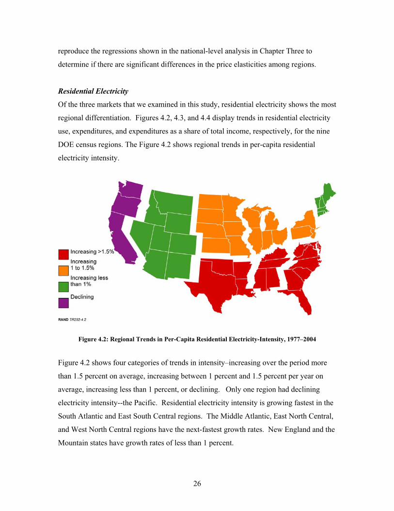
DOE census regions. The Figure 4.2 shows regional trends in per-capita residential

electricity intensity.

Figure 4.2: Regional Trends in Per-Capita Residential Electricity-Intensity, 1977–2004

Figure 4.2 shows four categories of trends in intensity–increasing over the period more

than 1.5 percent on average, increasing between 1 percent and 1.5 percent per year on

average, increasing less than 1 percent, or declining. Only one region had declining

electricity intensity--the Pacific. Residential electricity intensity is growing fastest in the

South Atlantic and East South Central regions. The Middle Atlantic, East North Central,

and West North Central regions have the next-fastest growth rates. New England and the

Mountain states have growth rates of less than 1 percent.

27

It is interesting to note that some commonality exists across contiguous regions. The

East South Central, West South Central, and South Atlantic regions have experienced the

most-rapid growth in electricity intensity, perhaps driven by air-conditioning loads and

rapidly growing populations. The Middle Atlantic and West North Central regions also

have had increasing air-conditioning loads at levels that did not exist until the late 1980s,

and they have seen relatively rapid growth in electricity intensity over this period.

The Pacific Coast, which is dominated by California in its magnitude of electricity use,

has had declining electricity intensity, possibly due to energy-related building codes that

are the strictest in the nation and have been in place longer than any others.

All of these findings might imply that the impact of energy efficiency would be greater in

areas such as the South in which the intensity of electricity use has been growing more

rapidly than in other regions and might have less of an impact in the Pacific Coast where

intensity has been declining.

Figure 4.3 shows growth trends for average expenditures on residential electricity. The

figure shows that average expenditures on residential electricity are growing in all

regions but provides a different picture than residential electricity intensity. Expenditures

are growing most rapidly in the South Atlantic, East South Central, New England, and

Pacific Coast regions. The Middle Atlantic and West South Central regions have the

next-fastest growth rate, while the Mountain, East North Central, and West North Central

regions have the slowest growth rates.

In a demand-price relationship, one might expect to see a picture similar to the one for

electricity intensity--those areas with the most rapid increases in expenditures would have

declining or slower growth in electricity intensity. While this is true for the Pacific states

and Northeast, the opposite is true for the South Atlantic and East South Central regions.

This is the first indication that the regional differences in the demand-price relationship

might matter when estimating the impact of energy efficiency on other demand changes.

28

Figure 4.3: Regional Trends in Average Expenditures on Residential Electricity, 1977–2004

We now look at average expenditures on residential electricity as a share of personal

income (see Figure 4.4). Although the spread of the numbers is small, there are a few

interesting findings to note. First, even though expenditures on electricity have been

rising, the share of electricity as a percentage of income has been declining, meaning that

incomes are growing faster than electricity use. In the Mountain and Northeast regions,

the relationship is what we would expect—where expenditures per dollar of income are

declining rapidly, electricity intensity is growing quickly. We would expect that where

the expenditures per dollar of income are declining more slowly than in other regions,

electricity intensity growth would be slower or declining (as is the case in the Pacific

Coast). But in the South Atlantic and East South Central regions, we find that even

though the expenditure per dollar of income is not declining as fast as that in other

regions, electricity intensity is growing more rapidly than in the other regions. This

finding might be an indication that electricity use in the South Atlantic and East South

Central regions is relatively insensitive to the cost of using electricity. At the very least, it

is another indication of regional diversity. We also see some commonality among

neighboring regions--for example, energy intensity in all the Southern regions is

declining more slowly than in other regions, while in the mid-Northern regions it is

declining more rapidly.

29

Figure 4.4: Regional Trends in Average Expenditures on Residential Electricity as a Share of

Income, 1977–2004

One might conclude from Figures 4.2 through 4.4 that there are regional differences in

the relationship between electricity demand and price and regional differences in the

trends in electricity usage and expenditures. Using the method described in Chapter

Two, we estimated the short-run and long-run price elasticities by region, which are

presented in Figures 4.5 and 4.6. We find that the regional estimates of short-run

elasticities range from -.04 in the East North Central region to .31 in the South Atlantic

region. We also present the 95 percent confidence interval for each of the regional

estimates. Where the confidence intervals do not overlap, we can say the regions are

significantly different from each other. Where they do overlap, there may be differences,

but, statistically, it is difficult for us to determine if they are actually distinct. In this

case, all the confidence intervals overlap to some extent, except for those for the South

Atlantic and East North Central estimates. Those two regions are the only ones that have

significant differences in elasticities.

Long-run demand (see Figure 4.6) is more elastic than short-run demand in each region,

and while the long-run pattern is relatively similar to the short-run pattern, the East South

Central region in this case is the most elastic, and the differences between the East South

30

Central and South Atlantic regions and the East North Central region are statistically

significant. The other regions differ from one another less for long-run elasticities than

they do for short-run elasticities.

Figure 4.5: Estimated Short-Run Residential-Electricity Price Elasticities by Region, 1977–2004

Figure 4.6: Estimated Long-Run Residential-Electricity Price Elasticities by Region, 1977–2004

31

When the various pieces of this analysis are brought together, they indicate that the

relationship between demand and price vary enough by region that estimates of future

residential electricity use or estimates of the impacts of energy-efficiency programs

should reflect some of the regional variation.

Commercial Electricity Results

While the analysis of the residential electricity sector showed significant regional

differences, the commercial electricity sector is somewhat less diverse. Our analysis of

commercial energy intensity found some differences across regions, but the elasticities

did not differ. The trend in electricity intensity per square foot of office space has been

moving toward increased intensity, with slower increasing rates in the Pacific Coast and

East South Central regions (see Figure 4.7). We cannot say that the Pacific Coast region

is statistically different from zero in terms of commercial electricity intensity, and the

West Southern Central and East Southern Central regions are significantly lower than

most of the other regions. This finding indicates that new newly constructed buildings

may be more energy efficient in some regions than in other regions. It may also indicate

that the impacts of future improvements in commercial electricity efficiency may be

larger regions with high growth in energy use, such as New England, the West North

Central, and the South Atlantic, and might have little additional impact on the Pacific

Coast region.

The short-run price elasticities for commercial electricity range from just under -.3 to -.15

(see Figure 4.8). Figure 4.8 indicates that some differences exist in short-run price

elasticity estimates across regions, but they are smaller than the differences in such

estimates across regions in the residential electricity sector. In addition, the commercial

electricity estimates have considerably greater variance (larger confidence intervals) than

the residential sector estimates. Given this large variance, there are no significant

differences among regions. Although we cannot say the regions are statistically different

from each other, it does appear that the Pacific Coast and East South Central regions are

32

somewhat more elastic in terms of commercial electricity than the other regions, and one

might look at these two regions somewhat differently than the others.

Figure 4.7: Regional Trends in Commercial Electricity Use per Square Foot of Office Space,

1977–1999

Figure 4.8: Short-Run Commercial Electricity Price Elasticities by Region, 1977–1999

33

Figure 4.9 shows that demand is more elastic in the long run than in the short run for the

commercial electricity sector, but there is even less variation among the regions. The

estimates shown in Figure 4.9 have large variances, and discerning differences in

elasticities among the regions is not possible.

What we can conclude from the above discussion is that there are not many regional

differences in commercial electricity use. Therefore, estimates of future electricity use at

the regional level will not be greatly impacted by dissaggregation to the regional level,

except perhaps for the Pacific Coast and East South Central estimates. Differences in

elasticities among states are still possible, and those differences are assessed in Chapter

Five.

Figure 4.9: Long-Run Commercial Electricity Price Elasticities by Region, 1977–1999

Residential Natural Gas

Our analysis of residential natural-gas energy intensity and expenditures on natural gas as

a share of income shows that there are differences in long-term trends among regions,

although the trends themselves are small in magnitude. Figures 4.10 and 4.11 show

34

intensity and price trends by region for natural gas. The largest increase in intensity is in

the Pacific Coast, driven by Washington and Oregon, and the greatest decline in intensity

is in the West South Central region, driven by Texas. There are large variations in the

estimates; therefore, for the most part, we cannot distinguish among trends in intensity in

the regions. Clearly, though, the Pacific Coast and Mid-Atlantic trends are positive, and

the rest are negative (with the New England trend being indistinguishable from zero).

This finding does suggest, however, that improvements in the efficiency of natural-gas-

using appliances might have a bigger impact in the Pacific Coast and Middle Atlantic

regions than they would in most other regions, and that additional improvements in the

energy efficiency of natural-gas-using appliances in the West South Central region may

have little impact.

Figure 4.10: Natural-Gas Intensity Trends by Region, 1977–2004

The price trends for natural gas provide an interesting picture of the demand-price

relationships one would expect. Increasing-price trends occurred in the regions with

declining natural-gas intensity; the Pacific Coast and New England regions, which had

increases in intensity, had an overall trend of prices not increasing (prices fluctuated

across the sample for all the regions, but in the Pacific Coast and New England regions,

35

the overall average trend was indistinguishable from zero). The sole exception to these

trends is the Middle Atlantic region, which had small increasing price trends and

increasing intensities. In Washington and Oregon, which were the primary drivers on the

Pacific Coast for the increasing intensity, there has been some substitution of natural gas

for electricity for heating purposes, some of which may have been driven by building

codes that encouraged shifts from electricity for water heating. These results certainly

indicate that some interesting results should be expected from the elasticity estimates.

Figure 4.11: Natural-Gas Price Trends by Region, 1977–2004

Short-run price elasticity for residential natural gas varies from –0.03 for the West South

Central region to –0.18 for the Pacific Coast (see Figure 4.12). The variance in the

estimates, as in the commercial sector, is large. The Pacific Coast, again, has the greatest

elasticity, and its neighboring Mountain region runs a close second. While we cannot say

that the elasticity in these two regions is significantly different from that of the other

regions, it may be worth further exploring benefits estimates for these two regions. Of the

contiguous regions, the southern-state regions are the least elastic, and the northern-state

regions are in the middle.

36

The long-run price-elasticity estimates (see Figure 4.13) are more elastic than the short-

term estimates, with the most inelastic region still the West South Central and the most

elastic still the Pacific Coast. While the variances are large in the long run, too, the

Pacific Coast and Mountain regions are close to being significantly different from the

West South Central, and there is a group in the middle with similar elasticities.

Figure 4.12: Short-Run Natural-Gas Price Elasticities by Region, 1977–2004

37

Figure 4.13: Long-Run Natural Gas Price Elasticities by Region, 1977–2004

The results for residential natural gas fall somewhere in between those for residential

electricity and those for commercial electricity in terms of regional differences. As was

the case with commercial electricity, there are few discernable differences in trends

among the regions, but there are more differences in the elasticities than in commercial

electricity, although still not at the level of significance that was seen in residential

electricity. It might make a difference in forecasts and estimates if the Pacific Coast and

Mountain regions are differentiated from the other regions.

Regional Analysis Conclusions

The analysis of regional-level differences in the price-demand relationship provides

different answers for different markets. It seems clear that there are regional differences

in the residential electricity market, and that estimates of the impact of energy efficiency

and forecasts of electricity demand could differ significantly if the regional differences

are taken into account. Clearly, commercial electricity does not appear to differ

significantly by region; therefore, national-level estimates of commercial electricity

price-demand relationships are likely to be sufficient for analyzing the impact of energy

efficiency in the commercial sector. The picture for residential natural gas is somewhat

38

different. There is not a lot of variability in energy-use trends over time, which is

probably why there is not much difference by region in the price-demand relationship. It

appears that demand responds more to price in two of the regions than in the others, and

this finding could have some implications for estimates of the benefits of energy

efficiency, but national level results in this case are probably also sufficient for analyzing

the impact of energy efficiency in the commercial sector

39

Chapter 5: State-Level Analysis

In this chapter, we use a methodology similar to the one that was used for the analysis in

the previous chapter, but in this case, we differentiate state-level elasticities and trends.

The state-level analysis consists of an examination of trends and an estimation of short-

run and long-run price elasticities for each state.

Residential Electricity

Beginning again with residential electricity, we look at the key trends in energy intensity

and expenditures as a share of income. In terms of electricity use per capita (see Figure

5.1), there are only a few states, which are concentrated in the West and New England,

with trends of small or declining energy intensity over the period studied. As we found

in the regional-level analysis, the high-growth areas in terms of residential electricity

usage are concentrated in the South. The significance of Figure 5.1 is in the consistency

it shows within regions. While the energy intensity trends do vary within each region,

they do not vary significantly. There are no regions with some states with declining

intensity and some states with rapidly increasing intensity. This is a first indication that

the regional-scale analysis might be sufficient for analyzing the impacts of energy

efficiency.

We do observe some inter-regional variation in electricity expenditures as a share of

income (see Figure 5.2). There is some diversity within each of the regions, although in

most cases, the differences among states in a region are small except for a single state.

Because the demand is consistent within regions, but the expenditures and prices are not,

the elasticities in states in each region might vary.

Next, we take a look at the differences in estimated residential electricity price

elasticities, which are illustrated in Figure 5.3. Each square-shaped plot point in the

figure represents a U.S. state, and the vertical lines represent the 95 percent confidence

interval. Sixteen states have an estimated elasticity that is positive over the period

studied, although the variance is large enough in most cases that it is difficult to

40

distinguish it from zero. There are a few possible explanations for this observation. In

the early years that were studied, when prices were rising, these states saw consistent

increases in demand, and in the later time period, when prices were declining in real

terms, these states did not have rapid growth in demand. Therefore, overall, it would

appear that the demand-price relationship reacts differently in these states than in other

states. We caution, however, that it is possible that in the future, increases in prices in

these states would not lead to increases in demand, but that the demand in these states

would indeed slow or decrease in a manner similar to that in other states (although the

elasticity might still be substantially less than that in other states).

Figure 5.1: State-Level Trends in Residential Electricity Intensity, 1977–2004

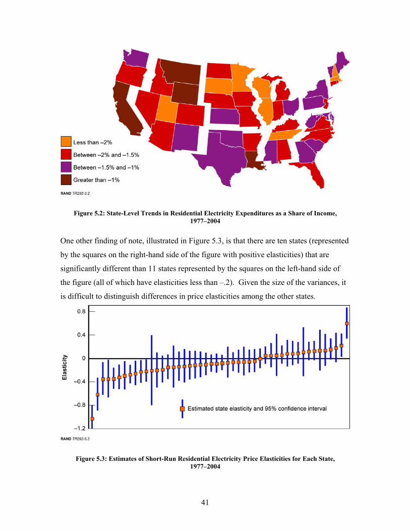
41

Figure 5.2: State-Level Trends in Residential Electricity Expenditures as a Share of Income,

1977–2004

One other finding of note, illustrated in Figure 5.3, is that there are ten states (represented

by the squares on the right-hand side of the figure with positive elasticities) that are

significantly different than 11 states represented by the squares on the left-hand side of

the figure (all of which have elasticities less than –.2). Given the size of the variances, it

is difficult to distinguish differences in price elasticities among the other states.

Figure 5.3: Estimates of Short-Run Residential Electricity Price Elasticities for Each State,

1977–2004

42

In Chapter Four, we illustrated significant differences in elasticities among regions.

When we look at the individual state elasticities, some consistencies within the regions

emerge. Figure 5.4 shows that several Mountain, West South Central, and West North

Central states appear to have similar lower-positive or higher-positive price elasticities

for residential electricity. Nevada, Idaho, Utah, Wyoming, Colorado, New Mexico,

Oklahoma, Kansas, and Nebraska form a block of states with very inelastic demand (or

estimated positive elasticities); the price-demand relationship in these states appears to be

somewhat similar. Another broad region with notable results falls in the middle of the

country and the Southeast. The group of states from Missouri to Florida has larger-than-

average price elasticities, with the East South Central and South Atlantic regions showing

some inter-regional inconsistencies. States within the Middle Atlantic region are

consistent in terms of elasticities, as are the states in the East North Central region (with

the exception of Wisconsin). This finding implies that even though there are

considerable differences among the states in price elasticities, there are some regional

consistencies. Therefore, disaggregation of data by region might still be sufficient for

energy-efficiency impact analyses.

As one might expect, the geographic patterns in long-run price elasticity estimates (see

Figure 5.5) are similar to those in the short-run price elasticity estimates. The Mountain

states have inelastic demand, whereas states in the South Atlantic and East South Central,

Pacific Coast, and New England region have more-elastic demand in the long run. The

variance in the long-run elasticity estimates is larger than in the short-run estimates, and

more states exhibit positive long-run price elasticities than positive short-run price

elasticities. Overall, these findings seem to indicate that over the time period studied,

electricity demand continued to rise in many of these states, regardless of price. Given

the prices and demand that were observed over this time period, it is not clear whether

any conclusions can be made about how long-run demand would react to price increases.

We can say, again, that there appear to be regional differences, but consistencies among

states within the regions, in the long-run price-demand relationship.

43

Figure 5.4: Estimated State-Level Short-Run Price Elasticities for Residential Electricity, 1977–2004

Overall, the findings presented in this section imply that while regional disaggregation

will be important for estimating future impacts of energy-efficiency technology and

forecasting demand for residential electricity, state-level disaggregation may not be

necessary for that purpose.

Figure 5.5: Estimated State-Level Long-Run Price Elasticities for Residential Electricity, 1977–2004

44

Commercial Electricity

The state-level analysis of the commercial electricity sector reveals a pattern of electricity

usage similar to that at the regional level – there seems to be some state-level variation in

electricity use patterns, but few differences in the price-demand relationship. Figure 5.6

shows trends in commercial electricity use per square foot of office space (i.e., the trends

in intensity). We see the slowest growth in electricity use in states in the West, although

a few of those states show a slow growth in intensity. There is some consistency in

intensity among states within regions. For the most part, states within a region fall into

one of two consecutive categories of growth. Again, this finding seems to indicate that

the regional analysis would be sufficient to capture any differences that might exist in

electricity intensity in the commercial sector.

The estimated elasticities in commercial-sector intensity are what we might expect from

the previous sets of analysis. Figure 5.7 shows the estimated state-level short-run

elasticities. There is not much variation across the states in intensity, except for a few that

are represented at the left side of the figure. For the most part, the estimated elasticities

range between –.5 and zero, with a few states with positive elasticity (that is not

significantly different from zero), and a few states that seem to have more-elastic

demand. It is interesting to note that for a large number of states, the variance is small,

which means that the elasticities are well estimated. This is in contrast to the residential

sector, in which the variance is large for a number of states. There is also more variation

among the states in the residential-sector analysis in comparison with the commercial-

sector analysis, which shows little variation among the states. We observed the same sort

of patterns for the long-run elasticities.

Clearly, there does not seem to be a reason to disaggregate the analysis for commercial

electricity to the state level.

45

Figure 5.6: Estimated State-Level Trends in Electricity Intensity in the Commercial Sector,

1977–1999

Figure 5.7: Estimated Short Run Elasticities in Electricity Intensity in the Commercial Sector at the

State Level, 1977–1999

46

Residential Natural Gas

Because the regional-level results for residential natural gas showed little regional

diversity and a lot of variance in the estimates, it is not surprising that we find basically

the same results at the state level. There are differences among states, which become

evident when looking at natural-gas intensity at the state level (see Figure 5.8). What is

also evident is that there is significant variation among states within regions, with the

notable exception of the East North Central and the West South Central, where the trends

in natural gas use per capita are fairly consistent. Otherwise, there is not much in the way

of observed patterns to note. There are more states in the North that have growing

natural-gas intensities, but a group of states in the South Atlantic (and Tennessee) also

have growing intensities.

Given these findings, it is not surprising that we also find some large differences among

the states in estimated short-run price elasticities for natural gas (see Figures 5.9a and

5.9b) along with very large variances among the states. The price elasticities range from

-.3 to .1, which is quite a broad range, but the variances are so large that we cannot even

say that states at the extreme low end of the range are statistically different from other

states. Reflecting what we observed at the regional level, there is not much in the way of

consistency among states within the regions in terms of price elasticity. There is a group

of contiguous states ranging from the middle of the country to the East Coast that have

some similarities in elasticities. But again, because the variances are so large, there is not

much we can interpret from these results, and there does not seem to be much of a reason

to assess natural-gas demand and the benefits of energy-efficiency technologies at the

state level.

47

Figure 5.8: Trends in Natural-Gas Intensity at the State Level, 1977–2004

Figure 5.9a: Estimated Short-Run Price Elasticities for Natural Gas at the State Level, 1977–2004

48

Figure 5.9b: Short-run Price Elasticities for Natural Gas

State-Level Conclusions

There are differences among the states in price elasticities and in some trends in energy

use and other factors, but, for the most part, they are not significant. As was seen with

the regional analysis, there is a difference between the results of the residential electricity

analysis and those of commercial electricity and residential natural-gas analyses. For

residential electricity use, there is enough consistency among states within regions that a

state-level disaggregation would not likely produce different results than would regional-

level analyses for forecasting the estimated benefits of energy-efficient technologies.

For commercial electricity and residential natural gas, there is not much consistency

among states, and there are significant amounts of variance in the estimates; therefore, it

is not certain that one could use our approach to differentiate states to a degree that would

be useful in forecasting estimates of energy-efficiency benefits.

49

Chapter 6: Utility-Level Analysis

The utility-level analysis posed a number of analytical challenges, which limited the

conclusions that we were able to draw from our analysis. While consumption and price

data at the utility level were available in the database that we used, data on other factors

that are key to the price-demand analysis (such as income and climate) were not. As such,

we used state-level data in place of the unavailable utility-level data. Nevertheless, we

continued with the experiment to see if there appear to be significant differences in how

price and demand respond at the utility-scale level, simply to glean whatever information

that might contribute to this study.

We did discover a few interesting things in this analysis. First, there is a lot of variation

in elasticities among the utilities, which was not unexpected, although the price

elasticities for about 65 percent of the sample are not statistically significant. Figure 6.1

illustrates the percentage of the sample of utilities that are in each region (shown in

Figure 4.1), and of those, the percentage with estimated price elasticities that are

statistically significant. There are no apparent regional consistencies, other than the

South Atlantic and East North Central regions having the highest percentage of utilities

with significant elasticities. For most regions, the percentage of utilities in the region and

the percentage with significant estimates are very similar. At one end, the East North

Central region had about 5 percent more utilities with statistically significant price

elasticities, as a proportion of all utilities in the dataset, than the region’s percent of the

total number of utilities in the data set, and the Mountain region had more than 5 percent

fewer utilities with statistically significant price elasticities.

The price-elasticity estimates are wide-ranging and have limited precision. The range of

elasticities for the statistically significant estimates was 1.1 to –1.87. The median was

–0.57, and the mean was –0.63.

Size of a utility appears to be correlated with the elasticity estimate. The range of

elasticity estimates for the largest utilities (the median is –0.25, and the mean is –0.29) is

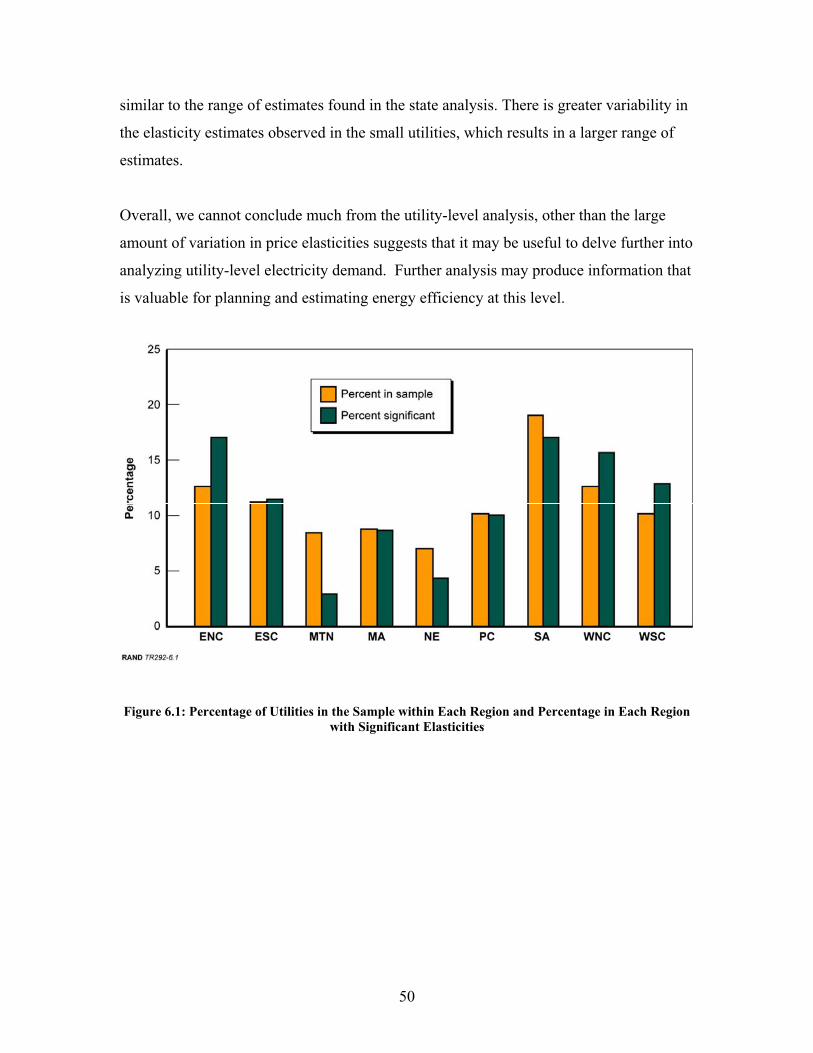
50

similar to the range of estimates found in the state analysis. There is greater variability in

the elasticity estimates observed in the small utilities, which results in a larger range of

estimates.

Overall, we cannot conclude much from the utility-level analysis, other than the large

amount of variation in price elasticities suggests that it may be useful to delve further into

analyzing utility-level electricity demand. Further analysis may produce information that

is valuable for planning and estimating energy efficiency at this level.

Figure 6.1: Percentage of Utilities in the Sample within Each Region and Percentage in Each Region

with Significant Elasticities

51

Chapter 7: Conclusions, Final Thoughts, and Implications of Analysis

This chapter reviews the results of our analysis and their implications and presents our

recommendations for further analysis. The key findings from this study are as follows:

• There are state and regional differences in (1) electricity and natural-gas demand,

(2) the relationship between changes in demand and changes in price (i.e.,

elasticity), and (3) factors that influence demand.

• It is difficult, with the data we have available, to show statistically significant

differences at all levels for commercial electricity and residential natural gas, though

our results do indicate there may be regional and state differences in how price and

demand interact in each of those sectors.

• We found significant regional differences in the price-demand relationship for

residential electricity, but also found consistencies in the price-demand relationship

for residential electricity among states within regions.

• The price-demand relationships have not changed over the past couple of decades—

our estimates are about the same as those from studies done in the 1980s.

• Price elasticity—-i.e., how demand reacts to changes in price overall—has

continued to be small since the 1980s.

• Over the periods we examined (1977–2004 for residential electricity and natural

gas, 1977–1999 for commercial electricity, and 1989–1999 for residential electricity

at the utility level), some basic trends emerged: Demand for energy overall is

increasing; in many cases, energy intensity is increasing, but price is decreasing;

and, while expenditures on energy are increasing, energy expenditures as a share of

consumers’ income and as a share of commercial sector output are declining.

• The past few years have seen some changes in these patterns, and it is possible that

some of these trends and relationships might exhibit further changes.

52

Should DOE Disaggregate Data for Estimating Energy-Efficiency Programs Benefits?

The results of this study have a number of implications for the DOE’s decisionmaking

and policymaking. The basic question that was the impetus for this analysis was whether

the DOE should disaggregate data (from the national level to the regional, state, or utility

level) when estimating the benefits of its energy-efficiency programs. The answer to this

question has a number of components.

We first made the case that certain factors might affect the impact that energy efficiency

would have on overall demand. We also made the case that the price-demand

relationship, or price elasticity, was important for estimating the impact of energy-

efficiency programs and technology. In examining demand in each sector (residential

and commercial electricity demand and residential natural-gas demand), we found that

there are some differences in regional trends—in particular, trends in the intensity of

energy use. Energy efficiency might have a bigger impact on regions with rapidly

growing intensity of use than on regions with intensity that is either declining or growing

slowly.

In terms of the price-demand relationship, if increasing prices motivate investments in

energy efficiency, then the impact of energy efficiency might be greater in regions or

states that are the most elastic (i.e., those with the lowest negative price elasticities). In

these regions and states, the price-demand relationship is the most robust, and changes in

price could lead to greater changes in energy efficiency, and vice-versa. Any estimates of

the impact of energy-efficiency programs will be impacted by price elasticity, and if the

elasticity differs significantly by region or state, the estimates of the impacts will differ

accordingly.

In the case of the residential electricity sector, it is clear that there are regional

differences. It also seems clear that the elasticities are relatively consistent among states

within the regions and that, at least for the near term, disaggregating data on energy-

efficiency programs to the regional level should be sufficient to evaluate the different

effects that energy efficiency could have in different regions of the country.

53

The results are less clear for the commercial electricity sector. Few regions appear to

have significantly different trends in the intensity of electricity use (specifically the

Pacific Coast and perhaps the West North Central and East South Central regions, which

have had slower growth). Statistically, it is difficult to distinguish among the other

regions in terms of intensity of use, and there are no discernable differences in the price

elasticities between regions. It does seem that the impact of energy efficiency in the

Pacific Coast would differ from the impact in the rest of the country, and perhaps

disaggregating Pacific Coast data from the national-level data is all that is needed to

estimate the impact of certain DOE programs. On the other hand, there is some

consistency in price elasticities among states within regions, such as what was seen in the

residential electricity sector, although not to as great an extent. This finding does suggest

that a state-level analysis would not be necessary in the short term.

The results are even less clear for the residential natural-gas sector. As in the commercial

sector, only a couple of regions (again, the Pacific Coast and the West South Central

region) seem to differ from the rest in all the factors we examined. But there is little

consistency in the states within the DOE regions and little statistical difference among the

estimated elasticities for each region. If one uses the estimated elasticities, the impact of

energy-efficiency programs in the Pacific Coast and in the West South Central region

would differ if one were to compare the two regions. This makes interpreting the findings

on residential natural gas use more difficult than interpreting the findings for the other

energy sectors. One finding of note is that the changes in demand for natural gas are

smaller than those for electricity over the time period studied, so perhaps national-level

analysis would be sufficient for determining the impact of energy-efficiency programs on

demand in the residential natural-gas market.

Price Elasticity of Demand

The results on price elasticity are interesting. Our elasticity estimates are no different

from those from ten to 20 years ago. This indicates that the relationship between price

and demand has not changed even though (1) 15 to 20 additional years of empirical data

54

are available; (2) there have been changes and shifts in energy use, in particular the

introduction of new electricity-using devices; (3) there have been large increases in air-

conditioning loads; and (4) appliances are more energy efficient than they were 15 to 20

years ago.

In addition, the elasticities remained the same over the past two decades—i.e., they

remained low. In other words, demand did not tend to react much to changes in price.

There are small, and somewhat consistent, changes, but on the surface it seems that there

are few options for consumers or commercial businesses to switch to electricity or natural

gas use in response to energy prices.

These observations, however, might be driven more by the trends in factors affecting

intensity than by how consumers react to changes in price. Over the time period studied,

we observed the following general trends:

• Energy prices heading downward

• Energy costs as a share of income also heading downward

• Energy use rising.

Given these trends, it is difficult to find significant variations in the price-demand

relationship, because prices and demand have not varied much. Also, it is difficult to

achieve improvements in energy efficiency when energy costs continue to decline,

beyond those that “naturally” occur through technology improvements.

On the other hand, it is possible that the price-demand relationship is changing. First, just

anecdotally, when California was facing energy problems in 2000 and 2001, a

combination of factors led to a significant reduction in residential electricity use, with

reductions in electricity demand estimated to be as high as 9 percent in response to

government policy, media coverage, and rising prices. At least in a case such as that,

consumers will change their demand behavior in the short term in response to energy

prices and energy policy.

55

In the past few years, we have witnessed a reversal of the downward price trends and, at

the same time, we have seen a reversal in the upward trend in electricity intensity in a

number of states. Overall, prices have not been declining as rapidly, and energy use has

not been increasing as rapidly either. So, it is possible that with an increasing-price

regime, one might see a different demand-price relationship than what would be observed

in a decreasing-price regime. More study and analysis would be needed to uncover these

trends.

57

Bibliography

Bentzen, Jan, and Tom Engsted, “A Revival of the Autoregressive Distributed Lag Model

in Estimating Energy Demand Relationships,” Energy, Vol. 26, 2001, pp. 45–55.

Bernstein, Mark, Kateryna Fonkych, Sam Loeb, and David S. Loughran, State-Level

Changes in Energy Intensity and Their National Implications, Santa Monica,

Calif.: RAND, MR-1616-DOE, 2003.

Bernstein, Mark, Robert J. Lempert, David S. Loughran, and David Ortiz, The Public

Benefit of California’s Investments in Energy Efficiency, Santa Monica, Calif.:

RAND, MR-1212.0-CEC, 2000.

Bohi, Douglas R. and Mary Beth Zimmerman, “An Update on Econometric Studies of

Energy Demand Behavior,” Annual Review of Energy, Vol. 9, 1984, pp. 105–154.

Dahl, Carol A., “Do Gasoline Demand Elasticities Vary?” Land Economics, Vol. 58, No.

3, August 1982, pp. 373–382.

Dahl, Carol A. and Thomas Sterner, “Analysing Gasoline Demand Elasticities: A

Survey,” Energy Economics, July 1991, pp. 203–210.

Dubin, Jeffrey A. and Daniel L. McFadden, “An Econometric Analysis of Residential

Electric Appliance Holdings and Consumption,” Econometrica, Vol. 52, No.2,

March 1984, pp. 345–362.

Garcia-Cerutti, L. Miguel, “Estimating Elasticities of Residential Energy Demand from

Panel County Data Using Dynamic Random Variables Models with

Heteroskedastic and Correlated Error Terms,” Resource and Energy Economics,

Vol. 22, 2000, pp. 355–366.

Griffin, James M., and Craig T. Schulman, “Price Asymmetry in Energy Demand

Module: A Proxy for Energy-Savings Technical Change,” The Energy Journal,

Vol. 26, No. 2, 2005, pp. 1–21.

Houthakker, H .S., Philip K. Verleger, Jr., and Dennis P. Sheehan, “Dynamic Demand

Analyses for Gasoline and Residential Electricity,” American Journal of

Agricultural Economics, Vol. 56, No. 2, May 1974, pp. 412–418.

Hsing, Yu, “Estimation of Residential Demand for Electricity with the Cross-Sectionally

Correlated and Time-wise Autoregressive Model,” Resource and Energy

Economics, Vol. 16, 1994, pp. 255–263.

58

Maddala, G. S, Robert P. Trost, Hongyi Li, and Frederick Joutz, "Estimation of Short-

Run and Long-Run Elasticities of Energy Demand from Panel Data Using

Shrinkage Estimators," Journal of Business & Economic Statistics, Vol. 15, No. 1,

January 1997, pp. 90–101.

Mead, Walter J., Timothy D. Mount, Richard L. Gordon, and A. Myrick Freeman III,

“Discussion on McDonald, Searl, Perry, Houthakker, Verleger, Jr., Sheehan, and

Wilson,” American Journal of Agricultural Economics, Vol. 56, No. 2, May 1974,

pp. 427–435.

North American Electricity Reliability Council, “2005 Summer Assessment: Reliability

of Bulk Electricity Supply in North America,” May 2005.

O’Neill, Brian C., and Mausami Desai, “Accuracy of Past Projections of U.S. Energy

Consumption,” Energy Policy, Vol. 33, 2005, pp. 979–993.

Pesaran, M. Hashem, and Ron Smith, “Estimating Long-Run Relationships from

Dynamic Heterogeneous Panels,” Journal of Econometrics, Vol. 68, 1995, pp.

79–113.

Taylor, Lester D., “The Demand for Electricity: A Survey,” The Bell Journal of

Economics, Vol. 6, No. 1, Spring 1975, pp. 74–110.

U.S. Department of Energy, National Transmission Grid Study, Washington, D.C.: DOE,

May 2002.

Wooldridge, Jeffrey, Econometric Analysis of Cross Section and Panel Data, Cambridge,

Mass.: MIT Press, 2002.

Wooldridge, Jeffrey, Introductory Econometrics: A Modern Approach, Cincinnati, Ohio:

South-Western College Publishing, 1994.

59

Appendix A: Details on the Methodology Used to Estimate Elasticities

The primary goal of this study is to measure how the energy-demand relationship varies

at different levels of spatial aggregation (i.e., at the national, regional, state, and utility

level). We model the demand relationship as a function of four components:

• measured variables that vary across states and within states over time—such as

energy prices, income, population, and climate

• fixed differences between states—unmeasured variables that do not change in the

study period but that differ across states

• an aggregate time trend—one that accounts for unmeasured variables common to

all states, such as federal policy

• a random error term that varies across and within states.

We estimate this model with the following fixed-effects specification:

QD

i,t = QD

i,t-1 + Xi,t + Xi,t-1 + si + yt + i,t

where QD

i,t is log energy demand in state i and year t, QD

i,t is the lag value of log energy

demand, Xi,t is a set of measured covariates (e.g., energy prices, population, income, and

climate) that affect energy demand, and Xi,t-1 is the lag values of the covariates. The

residual has three components:

• si is an indicator variable that captures time-invariant differences in energy

demand across states (“state fixed effects”).

• yt is an indicator variable that captures time effects common to all states (“year

fixed effects”).

• i,t is a random error term.

We based this specification on the flow-adjustment model developed by Houthakker et

al. (1974). In this model, demand is a function of prices, income, population, and climate.

QD*

i,t = f(Pi,t, PC

i,t, Yi,t, Popi,t, Climatei,t)

where QD*

denotes desired demand in time t. The model assumes the following

adjustment process between periods:

QD

i,t/ QD

i,t-1 = (QD*

i,t/ QD

i,t-1)

where 0< < 1. The estimating equation then becomes the following:

60

ln QD

i,t - lnQD

i,t-1 = lnQD*

i,t - lnQD

i,t-1

ln QD

i,t = lnQD*

i,t + lnQD

i,t-1 - lnQD

i,t-1

ln QD

i,t = lnQD*

i,t + (1- ) lnQD

i,t-1

Then, by substituting in a linear function for QD*

i,t , the final form is the following:

ln QD

i,t = ln + ln pi,t + ln Xi,t + ln Xi,t-1 + (1- ) ln QD

i,t-1.

In this model, the term reflects that current demand (QD

i,t)adjusts partially to changes in

desired demand (QD*

i,t). Energy demand does not fully adjust in the current period

because it is a stock-flow process. In this stock-flow process, adjusting the stock usually

takes more than one period but consumers can control the flow easily in the current

period. Therefore, demand does not fully adjust within one period to changes in desired

demand.

In more tangible terms, the “stock” refers to energy-consuming appliances that a

consumer owns, such as a car, air conditioner, heater, and stove. The flow is the amount

that the consumer uses the appliance. In this process, the consumer has immediate

control over where the thermostat is set or how much he or she drives the car but these

decisions can only affect energy consumption to a limited degree. If the consumer wants

larger changes in energy demand, he or she must replace an expensive item like a car,

heater, or air conditioner, which typically cannot happen immediately.

This explanation for the partial-adjustment process suggests that an ideal model for

energy demand would explicitly represent consumer decisions on purchasing energy-

consuming appliances and their levels of usage. Taylor (1975) discusses this issue and

notes that most studies at that time had insufficient data on appliance purchases and usage

to estimate such a model. Other studies have estimated price elasticity using models of

this type, such as Dubin and Macfadden (1984). However, data limitations precluded

estimating a similar model for different spatial scales. Therefore, we proceeded with

Houthakker et. al.’s reduced-form model, which is commonly used in the literature.

By estimating the adjustment process ( ), we can estimate both short-run and long-run

price elasticities. The short-run price elasticity is the long-run price elasticity ( )

multiplied by the adjustment factor ( ), which in this model refers to , the estimated

coefficient on the current period price variable. The long-run elasticity is estimated by

subtracting the coefficient on the lagged demand variable (1- ) from one to get an

estimate of and then dividing the coefficient of the current price ( ) by the estimate of

.

We estimate any spatial differences in the energy-demand relationship by adding

interaction terms between indicator variables for the spatial unit of interest (region, state,

or utility) and the regressors of interest (price, quantity, and income). These interaction

61

terms allow the estimated parameters to vary, and we can analyze if price elasticities

differ across geographical units.

Parameter Identification

The variables of interest in this study, energy price and quantity, are jointly determined

by the interaction of energy supply and demand, which creates problems for identifying

parameters in the demand equation. Ideally, we would model the energy market with a

system of equations for supply and demand. With a system of equations, we could

isolate movements in the demand and supply curves and use this variation to estimate the

parameters in each equation. We were unable to develop a system of equations for each

spatial level used in the study and instead used a reduced-form model that can identify

the parameters of the demand equation under the following assumptions:

• the model includes all the factors that affect energy demand

• price changes between periods are exogenous

• the error term does not contain autocorrelation

The following discussion explains why these assumptions are necessary and then

examines their plausibility.

The first assumption is necessary because identifying parameters of the demand equation,

and more specifically the effect of prices on quantity, requires holding the demand curve

fixed and allowing shifts in the supply curve to establish the shape of the demand curve.

If the model was missing a factor that affected demand, then shifts in both demand and

supply could cause the observed shifts in price and quantity but the model would attribute

the changes solely to shifts in supply. More simply, the estimates in the demand equation

could suffer from omitted variables bias.

The second assumption is required to isolate the effect of price on demand. In a full

system of equations, changes in price affect demand and feed back into the supply

equation. Therefore, prices are endogenous and determined by the equilibrium between

supply and demand. Without a supply equation to capture this feedback, the model

cannot identify the parameter on the endogenous variable, unless prices enter the system

exogenously. The following discussion will examine some situations where prices could

plausibly enter the system as an exogenous variable.

The final assumption is needed because the lagged demand term can be written as a

function of past values of the error term. If autocorrelation is present, it creates

correlation between the error term and the lagged demand variable, which biases

estimates of the coefficient on lagged demand. The equations below show how

autocorrelation is a problem.

62

The model equation is:

QD

i,t = QD

i,t-1 + Xi,t + Xi,t-1 + si + yt + i,t

which can be re-written as:

QD

i,t = (QD

i,t-2 + Xi,t-1 + Xi,t-2 + si + yt + i,t-1) + Xi,t + Xi,t-1 + si + yt + i,t

By continuing to substitute for the lagged demand term, this term could be re-written as a

function of initial demand, lagged values of explanatory factors, and, most importantly,

past values of the error term. Therefore, any autocorrelation in the error term (E( i,t, i,s)

0 where t s) will create correlation between the lagged demand term and the error

term, which will bias estimates of the coefficient on lagged demand, .

The assumptions stated above for parameter identification are strong but not implausible.

The following discussion addresses each assumption.

Assumption #1 - Controlling for all factors affecting demand

The model includes the own-price of the good, price of a substitute, and income, which

are key variables in microeconomic decisions of demand. The model also controls for

population and climate, which would also affect energy demand. In addition, the model

includes lagged values of these factors, which controls for large period-to-period changes

in explanatory variables. The model also controls for demand in the previous period,

which in effect controls for the stock of energy-consuming appliances because the stock

of appliances is unlikely to change significantly from year-to-year. Finally, the model

includes fixed-effects for each cross-sectional unit and year.

The fixed-effects control for any unmeasured time-invariant effects on demand

attributable to the cross-sectional unit. An example of an unmeasured time-invariant

effect is energy demand patterns in states with federally-administered hydroelectric

power sectors. Washington, Oregon, and Tennessee have exceptionally high per capita

electricity use and low average prices. Some of this effect is due to prices, but each of

these states have electricity markets dominated by large federal power agencies that have

historically supplied the regions with inexpensive energy. The effect of these agencies is

difficult to measure, and is likely to differ between states. Therefore, including an

indicator variable for each state controls for the unique effects that agencies like the

Bonneville Power Administration or Tennessee Valley Authority have on energy

demand. In addition, the indicator variable controls for any other unmeasurable variables

that affect energy demand. The year fixed effects control for any year-to-year variation

in demand that occurs across all cross-section units. Examples of these effects are

national legislation, macroeconomic trends, and national-level events that affect energy

demand (war or terrorism attack).

The explanatory variables comprise a relatively comprehensive set of control variables

for energy demand. The very high R2 values (> 0.9) on the regressions indicate that the

63

model fits the data well and explains a large amount of the variation in energy demand.

One area where the model does not control for changes in demand is a state- or cross-

section specific factor that changes over time. For instance, if a subset of states

substantially changes their stock of energy-consuming appliances, then the model may

not control for this change in demand. This situation contrasts with national consumer

trends in purchasing new electronics, which the model can control for with year fixed

effects.

Assumption #2 – Exogenous energy prices

The assumption of exogenous energy prices is the strongest assumption but not

implausible. A public utilities commission that sets consumer rates regulates most

electricity and natural gas rates. These price schedules do not change regularly and the

rate setting is not exogenous. Despite these shortcomings, there are portions of a

consumer’s utility bill that do vary annually and this source of variation is arguably

exogenous. Most utility bills contain a component that passes through changes in fuel

prices to customers. Since utility rate schedules do not change regularly, much of the

period-to-period variation in what consumers actually pay for electricity and natural gas

is fluctuations in the fuel cost. Because these fuels are typically purchased at prices

determined on national or world markets, the change in prices from fuel costs is primarily

exogenous variation.

Assumption #3 – No autocorrelation in the error term

The discussion above showed that estimating the model with ordinary least squares

(OLS) when autocorrelation is present will result in biased estimates. This assumption is

testable and autocorrelation tests are performed on the regressions in the study. Alternate

estimation methods are possible, notably instrumental variables and error component

technique. In previous work, Houthakker et. al. (1974) found that OLS estimates with

separate intercepts for cross-section units (fixed-effects) produced estimates that were

comparable to the error component technique. Although, this finding is not generalizable

to other data sets. Therefore, this analysis includes tests for autocorrelation.

We follow the test for first-order autocorrelation discussed in Wooldridge (1994; 2002).

In this test, we run an OLS regression of the dependent variable on the explanatory

variables and obtain the residuals. We then run an OLS regression of the residuals on the

explanatory variables and lagged residuals. The coefficient on the lagged residual term is

a consistent estimate for and the t-statistic on the coefficient of the lagged residual term

is a valid test for the null hypothesis = 0 (no autocorrelation), where represents the

coefficient on the lagged error in an AR(1) model. In our results, we present the estimate

of and the associated t-statistic.

As stated earlier, an ideal model would include a system of equations to model the

demand and supply equations of each state’s energy market. The limited scope of this

study excluded an extensive analysis of supply and demand in each state. We followed

Houthakker’s demand model because it was widely used in the literature, we could

64

estimate differences in short- and long-run elasticities, and determine if these parameters

vary geographically. Under the assumptions stated above, the model will estimate the

causal effect of prices on energy demand—the focus of this study and measure how this

effect varies geographically. If these conditions are not met, the estimate will reflect the

correlation between the observed prices and quantities

Trend Analysis

The regional data analysis for each energy market in Chapter Four displays regional

trends for residential electricity, commercial electricity, and natural gas intensity,

expenditures, and expenditures as a share of income. We estimate these trends using a

deterministic time trend of the following form:

Ln dependent variable = 0 + 1 year +

This model fits a linear time trend to our data. In most of the analyses done for this

study, the trends were linear, and the model was a good fit, which was evidenced by R2

over 0.9 (the time trend). Appendix D displays the results from the trend analysis.

65

Appendix B: Data Sources

The regression analyses done for this study used panel data for the 48 contiguous states.

The time periods for each energy market analysis varied because of data limitations. The

data on the residential electricity and natural gas markets spans 1977 to 2004. The data

on commercial electricity extends only from 1977 to 1999. The data are from the

following four sources: the DOE EIA, Bureau of Economic Analysis (BEA) of the

Department of Commerce, the U.S. Census Bureau, and the National Oceanic and

Atmospheric Administration (NOAA).

Energy Data

The sources for electricity data include the following EIA publications: State Energy

Data Report 2001, Electric Power Annual, and Electric Power Monthly. By combining

these data sources, we developed a state-level database of electricity consumption and

prices for residential and commercial customers. The sources of natural-gas data include

the following EIA publications: State Energy Data Report 2001, Natural Gas Annual,

and Natural Gas Monthly. As was done for the electricity sector, for natural gas we

created a state-level database on consumption and prices for residential customers.

Economic Data

We obtained economic data on gross state product, GDP deflator, and population from

the Department of Commerce Bureau of Economic Analysis (BEA) “Regional Economic

Accounts” Web site (see http://www.bea.gov/bea/regional/data.htm). We purchased data

on commercial floorspace from McGraw-Hill Construction Dodge

(http://dodge.construction.com).

Climate Data

The NOAA publishes state-level data on heating and cooling degree days. The degree-

day measures quantify how far the daily average temperature deviates from 65 degrees.

For instance, if a day’s average temperature is 50 degrees, then the day has 15 heating

degree days. If the average is 70, then the day has five cooling degree days. We

constructed an annual climate index by summing heating and cooling degree-day

measures, which captures annual climate variation in each state. The data on degree days

are available on the NOAA website

(http://lwf.ncdc.noaa.gov/oa/documentlibrary/hcs/hcs.html).

66

67

Appendix C: Variables and How They Were Constructed

Table C.1: Residential Electricity Regression Analysis Variables

Variable How Variable Was Constructed/Data Source

Residential electricity consumption Electricity consumption (Btus), residential sector (ESRCB), 1977-1999

Source: EIA State Energy Data Report (2001)

Electricity sales (megawatt hours), residential consumers, 2000-2004

Source: EIA Electric Power Annual (2003) and Electric Power Monthly (2004)

Real residential electricity prices = Average price of electricity, residential sector (ESRCD), 1997-1999

Nominal residential electricity price / GDP deflator

Source: EIA State Energy Price and Expenditure Report (2001)

Average price of electricity, residential consumers, 2000-2004

Source: EIA Electric Power Annual (2003) and Electric Power Monthly (2004)

Real residential natural gas prices Average price of natural gas, residential sector (NGRCD), 1997-1999

Nominal residential natural gas price / GDP deflator

Source: EIA State Energy Price and Expenditure Report (2001)

Average price of natural gas, residential consumers, 2000-2004

Source: EIA Natural Gas Annual (2003) and Natural Gas Monthly (2004)

Population State population

Source: BEA, Regional Accounts Data, "Annual State Personal Income," Population table (no date)

Real disposable income per capita = Disposable income per capita

Disposable Income per capita / GDP deflator

Source: BEA, Regional Accounts Data, "Annual State Personal Income," Per capita disposable personal income table (no date)

Climate index = Heating degree days, cooling degree days

Heating degree days + Cooling degree days

Source: NOAA, National Climatic Data Center, "Heating and Cooling Degree Data" (no date)

68

Table C.2: Commercial Electricity Regression Analysis Variables

Variable How Variable Was Constructed/ Data Source

Commercial electricity consumption Electricity consumption (Btus), commercial sector (ESCCB) 1977-1999

Source: EIA State Energy Data Report (2001)

Real Commercial Electricity Prices = Average price of electricity, commercial sector (ESCCD) 1997-1999

Nominal commercial electricity price / GDP deflator

Source: EIA State Energy Price and Expenditure Report (2001)

Real Commercial Natural Gas Prices Average price of natural gas, commercial sector (NGCCD) 1997-1999

Source: EIA State Energy Price and Expenditure Report (2001)

Area of commercial floorspace Data purchased from McGraw-Hill Construction Dodge

http://dodge.construction.com/—includes data on square footage of commercial floor space from 1977 - 1999 for each sate

Real gross state product = Gross state product

Gross state product / GDP deflator Source: BEA, Regional Accounts Data, "Gross State Product," (no date)

Climate index = Heating degree days, Cooling degree days

Heating degree days + Cooling degree days

Source: NOAA, National Climatic Data Center, "Heating and Cooling Degree Data" (no date)

69

Table C.3: Residential Natural-Gas Regression Analysis Variables

Variable How Variable Was Constructed/ Data Source

Residential natural gas consumption Natural gas consumption (Btus), residential sector (NGRCB) , 1977-1999

Source: EIA State Energy Data Report (2001)

Natural gas sales (thousands of cubic feet), residential consumers, 2000-2004

Source: EIA Natural Gas Annual (2003) and NaturalGas Monthly (2004)

Real residential natural gas prices = Average price of natural gas, residential sector (NGRCD) 1997-1999

Nominal residential natural gas price / GDP deflator

Source: EIA State Energy Price and Expenditure Report (2001)

Average price of natural gas, residential consumers, 2000-2004

Source: EIA Natural Gas Annual (2003) and Natural Gas Monthly (2004)

Real residential electricity prices = Average price of electricity, residential sector (ESRCD) 1997-1999

Nominal residential electricity price / GDP deflator

Source: EIA State Energy Price and Expenditure Report (2001)

Average price of electricity, residential consumers, 2000-2004

Source: EIA Electric Power Annual (2003) and Electric Power Monthly (2004)

Population State population

Source: BEA, Regional Accounts Data, "Annual State Personal Income," Population table (no date)

Real disposable income per capita = Disposable income per capita

Disposable income per capita / GDP deflator

Source: BEA, Regional Accounts Data, "Annual State Personal Income," Per capita disposable personal income table (no date)

Climate index = Heating degree days, cooling degree days

Heating degree days + Cooling degree days

Source: NOAA, National Climatic Data Center, "Heating and Cooling Degree Data" (no date)

70

71

Appendix D: Regression Analysis Results

In this appendix, we present the results from regression analysis at the national, regional,

state, and utility levels of aggregation. We display the results for each energy market by

level of aggregation.

National-Level Results

This section shows results for the residential electricity, commercial electricity, and

residential natural gas markets. In the national level regressions, we estimate the model

using panel data from the 48 contiguous states. We estimate the following model for

these regressions:

QD

i,t = QD

i,t-1 + Xi,t + Xi,t-1 + si + yt + i,t

where QD

i,t is log energy demand in state i and year t, QD

i,t is the lag value of log energy

demand, Xi,t is a set of measured covariates (e.g. energy prices, population, income, and

climate) that affect energy demand, and Xi,t-1 is the lag values of the covariates. The si

term is a state-fixed effect estimated with an indicator variable. The yt term is a year-

fixed effect also estimated with an indicator variable and i,t is a random error term.

Residential Electricity

The dependent variable in this regression was the log of electricity sold to residential

electricity consumers. We controlled for the following variables:

• Lag value of dependent variable

• Log of residential electricity price

• Lag value of log of residential electricity price

• Log of per capita income

• Lag value of log of per capita income

• Log of state population

• Lag value of log of state population

• Log of residential natural gas price

• Lag value of log of residential natural gas price

• Log of climate index (heating degree days + cooling degree days)

The residential electricity market regression analysis covers the period from 1977-2004.

The data from 2001 are excluded from the analysis because EIA had serious errors in the

data for that year, which they have not corrected yet.

The results show that lagged quantity has a significant and positive effect on current

period consumption. Current and lagged electricity prices are significant and negative.

The estimates indicate that short run price elasticity (-0.24) is inelastic and similar to

previous estimates in the literature. The income, population, and natural gas variables are

72

all insignificant in the current period and significant in the lagged period. The lagged

values are all positive, which is expected. Income and population increases should

correspond with greater electricity demand. In this case, we consider natural gas a

substitute for electricity and the positive sign for the cross-price elasticity indicates it is a

substitute. Finally, the climate index has a significant and positive effect on residential

electricity demand.

Table D.1: Regression results from the residential electricity market

Robust

Coef. Std. Err. t P>|t| [95% Conf. Interval]

Lag quantity 0.232 0.058 4.03 0 0.119 0.345

Ln elec price -0.243 0.049 -4.96 0 -0.339 -0.147

Lag elec price -0.129 0.048 -2.7 0.007 -0.222 -0.035

Ln income 0.003 0.076 0.04 0.968 -0.146 0.152

Lag income 0.384 0.073 5.27 0 0.241 0.527

Ln population -0.225 0.285 -0.79 0.43 -0.783 0.334

Lag population 0.827 0.307 2.69 0.007 0.225 1.428

Ln nat gas price -0.005 0.028 -0.16 0.873 -0.06 0.051

Lag nat gas price 0.111 0.031 3.58 0 0.05 0.172

Ln climate 0.246 0.026 9.36 0 0.194 0.298

R2 = 0.99

N = 1237

The adjusted R-squared for this model is very high—approximately 0.99. A high R-

squared is typical with fixed effects models because the state and year effects included in

the model usually have considerable explanatory power.

We tested for first-order autocorrelation in the error term. The estimate of was -0.009

with a t-statistic of -0.69, which indicates first-order correlation is not present. We,

therefore, conclude that autocorrelation does not affect consistency of the coefficient

estimates or validity of the standard errors.

Commercial Electricity

The dependent variable in this regression was the log of electricity sold to commercial

electricity consumers. We controlled for the following variables:

• Lag value of dependent variable

• Log of commercial electricity price

• Lag value of log of commercial electricity price

• Log of gross state product

• Lag value of log of gross state product

• Log of commercial floorspace

• Lag value of log of commercial floorspace

73

• Log of commercial natural gas price

• Lag value of log of commercial natural gas price

• Log of climate index (heating degree days + cooling degree days)

Table D.2: Regression results from the commercial electricity market

Robust

Coef. Std. Err. t P>|t| [95% Conf. Interval]

Lagged quantity 0.785 0.034 22.81 0 0.717 0.852

Ln elec price -0.209 0.060 -3.47 0.001 -0.327 -0.091

Lag elec price 0.148 0.052 2.85 0.004 0.046 0.250

Ln nat gas price -0.023 0.020 -1.18 0.236 -0.061 0.015

Lag nat gas price 0.049 0.022 2.19 0.029 0.005 0.093

Ln commercial GSP 0.155 0.124 1.25 0.211 -0.088 0.398

Lag commercial GSP -0.039 0.122 -0.32 0.747 -0.279 0.200

Ln floorspace 0.504 0.339 1.49 0.138 -0.162 1.169

Lag floorspace -0.421 0.305 -1.38 0.169 -1.020 0.179

Ln climate 0.233 0.039 5.92 0 0.156 0.310

R2= 0.99

n = 1034

The commercial electricity market regression analysis covers the period from 1977-1999.

Later data are not included in the analysis because of consistency problems with gross

state product data collected by the Bureau of Economic Analysis. In addition, data from

Tennessee were excluded from this regression.

The results show that lagged quantity has a significant and positive effect on current

period consumption. The magnitude is larger than the estimate for residential electricity.

Current electricity price is significant and negative. The estimate indicates that short run

price elasticity (-0.21) is also inelastic and similar to previous estimates in the literature.

The lagged electricity price is positive and significant, which is not expected. The

estimates for natural gas are insignificant for the current period and significant and

positive for the lag period. Again, this suggests that natural gas is a substitute but the

cross price elasticity is small. All of the GSP and floorspace variables were insignificant.

Finally, the climate index has a significant and positive effect on commercial electricity

demand. The magnitude is also similar to the residential electricity estimate.

The adjusted R-squared for this model is also very high—approximately 0.99. This,

again, indicates the state and year effects included in the model have considerable

explanatory power.

We also tested for first-order autocorrelation in the error term. The estimate of was

0.021 with a t-statistic of 0.47. These results suggest first-order correlation does not

affect the coefficient estimates and standard errors in this model.

74

Residential Natural Gas

The dependent variable in this regression was the log of natural gas sold to residential

natural gas consumers. We controlled for the following variables:

• Lag value of dependent variable

• Log of residential natural gas price

• Lag value of log of residential natural gas price

• Log of per capita income

• Lag value of log of per capita income

• Log of state population

• Lag value of log of state population

• Log of residential electricity price

• Lag value of log of residential electricity price

• Log of climate index (heating degree days + cooling degree days)

Table D.3: Results from natural gas market regression analysis

Coef. Std. Err. t P>|t| [95% Conf. Interval]

Lag quantity 0.577 0.024 24.44 0 0.531 0.623

Ln nat gas price -0.132 0.031 -4.24 0 -0.193 -0.071

Lag nat gas price -0.106 0.031 -3.42 0.001 -0.167 -0.045

Ln elec price 0.034 0.053 0.64 0.521 -0.070 0.138

Lag elec price 0.146 0.052 2.8 0.005 0.044 0.248

Ln income 0.261 0.123 2.13 0.034 0.020 0.503

Lag income 0.167 0.113 1.48 0.139 -0.054 0.388

Ln population 1.169 0.449 2.6 0.009 0.287 2.051

Lag population -0.717 0.449 -1.6 0.11 -1.598 0.163

Ln climate 0.181 0.042 4.29 0 0.098 0.264

R2 = 0.96

n = 1210

The residential natural gas market regression analysis covers the period from 1977-2004.

The regression includes data from all time periods. It excludes the state of Maine from

the analysis. Gas volumes sold in Maine are very small in absolute terms and relative to

all other states. Since the absolute volumes traded are small, small changes had large

effects in % changes and disproportionately affected the price elasticity estimates. Since

the market there is small compared to the rest of the country, the analysis excludes it.

The results show that the lagged quantity is significant and the magnitude is similar to the

estimate in commercial electricity. Natural gas price is significant and negative in the

current and lagged period. The estimate of short-term price elasticity is –0.132, which is

smaller in absolute value than the estimates for both electricity markets. The current

price of electricity is insignificant but the lagged value is positive and significant. This is

further evidence that electricity and natural gas are substitutes for residential consumers.

75

The magnitude of the cross price elasticity is also small in this case. The estimates for

income and population are positive and significant in the current period but insignificant

in the lagged period. The elasticity for population (1.17) is large relative to the other

estimates, which indicates population change has a strong effect on demand in this

market.

The adjusted R-squared for this model is again very high—approximately 0.96. The

fixed effects included in the model also have considerable explanatory power for this

market.

We tested for first-order autocorrelation and found that it may be present in the error

term. The estimate of was -0.342 with a t-statistic of -6.75. Based on this result, we

estimated the model assuming an AR(1) structure in the error term, which should correct

the standard errors. However, autocorrelation still affects consistency of the estimate on

the lagged demand term.

Regional-Level Results

This section shows regional level results for the residential electricity, commercial

electricity, and residential natural gas markets. In the regional level regressions, we

estimate the model using panel data from the 48 contiguous states. We estimate the

following model for these regressions:

QD

i,t = QD

i,t-1 + Xi,t + Xi,t-1 + (ri x QD

i,t-1) Q + (ri x ln elec pricei,t) P +

(ri x ln incomei,t) I + si + yt + i,t

where QD

i,t is log energy demand in state i and year t, QD

i,t is the lag value of log energy

demand, Xi,t is a set of measured covariates (e.g. energy prices, population, income, and

climate) that affect energy demand, and Xi,t-1 is the lag values of the covariates. The

interaction terms interact a region indicator variable with lagged quantity, current prices,

and current income. The corresponding region-specific coefficient estimates are ( + Q )

for lagged quantity, ( P + P) for prices, and ( I + I) for income. The si term is a state-

fixed effect estimated with an indicator variable. The yt term is year-fixed effect also

estimated with an indicator variable and i,t is a random error term.

Residential Electricity

The table shows that demand response in the South Atlantic and East South Central is

most elastic and the East North Central has the most inelastic demand response. All of

the estimates are negative and statistically significant, except the East North Central. The

estimates also indicate regional differences in electricity demand. The estimates for the

South Atlantic and East South Central have statistically significant differences from the

East North Central. A Wald Test on the South Atlantic and East North Central

coefficients rejects the null hypothesis that they are equal (F(1,1130) = 14.59; p =

0.0001). A Wald Test on the East South Central and East North Central coefficients also

76

rejects that they are equal (F(1,1130) = 10.37; p=0.0013). Overall, the regression results

show clear statistically significant differences in price elasticities between the regions.

Table D.4: Estimated short-run price elasticities for the residential electricity market

Short run price elasticity

Coef. Std. Err. t P>|t| [95% Conf. Interval]

South Atlantic -0.318 0.047 -6.77 0 -0.41 -0.226

East South Central -0.266 0.071 -3.74 0 -0.405 -0.126

Mid Atlantic -0.232 0.069 -3.36 0.001 -0.368 -0.096

Mountain -0.211 0.038 -5.55 0 -0.285 -0.136

New England -0.192 0.046 -4.2 0 -0.281 -0.102

Pacific Coast -0.188 0.051 -3.69 0 -0.288 -0.088

West North Central -0.163 0.054 -3.02 0.003 -0.269 -0.057

West South Central -0.127 0.051 -2.52 0.012 -0.227 -0.028

East North Central -0.054 0.053 -1.01 0.312 -0.158 0.051

We tested for first-order autocorrelation in the error term and the estimate of was -0.003

with a t-statistic of -0.26. The estimate indicates that first-order autocorrelation does not

affect the error term and this model. Therefore, autocorrelation does not affect the

estimate of lagged demand and the inference based on the standard errors is valid.

Table D.5: Estimated long-run price elasticities for the residential electricity market

Coef. Std. Err. t P>|t| [95% Conf. Interval]

East South Central -0.618 0.144 -4.3 0 -0.900 -0.336

South Atlantic -0.352 0.051 -6.86 0 -0.453 -0.251

New England -0.325 0.074 -4.37 0 -0.471 -0.179

Mountain -0.267 0.048 -5.52 0 -0.362 -0.172

Pacific Coast -0.254 0.078 -3.27 0.001 -0.407 -0.101

Mid Atlantic -0.247 0.075 -3.28 0.001 -0.395 -0.099

West North Central -0.244 0.081 -3.01 0.003 -0.403 -0.085

West South Central -0.174 0.070 -2.48 0.013 -0.311 -0.036

East North Central -0.058 0.057 -1.02 0.309 -0.169 0.054

Long run price elasticities are calculated by dividing the coefficient estimate on current

electricity prices by 1 – the coefficient of lagged quantity. The long-run elasticities are

larger for all of the regions, which is expected and follows the general findings from

previous research. The pattern of results is also similar to the short-run elasticity results.

The East South Central and South Atlantic regions have the most elastic demand and the

East North Central is the most inelastic. Again, all of the estimates have the expected

sign and significant, except for the East North Central.

77

Commercial Electricity

We used the same regression model to estimate the regional-level commercial electricity

market.

Table D.6: Short-run price elasticities for commercial electricity with and without Tennessee

Short-Run Price Elasticity – with Tennessee

Coef. Std. Err. t P>|t| [95% Conf. Interval]

East South Central -0.759 0.322 -2.36 0.019 -1.391 -0.127

Pacific Coast -0.364 0.099 -3.67 0 -0.559 -0.169

New England -0.273 0.101 -2.71 0.007 -0.470 -0.076

Mountain -0.258 0.126 -2.04 0.042 -0.505 -0.010

West South Central -0.250 0.114 -2.19 0.029 -0.475 -0.026

East North Central -0.237 0.111 -2.13 0.033 -0.455 -0.019

West North Central -0.233 0.132 -1.76 0.078 -0.491 0.026

South Atlantic -0.226 0.106 -2.13 0.034 -0.435 -0.017

Mid Atlantic -0.215 0.081 -2.64 0.009 -0.374 -0.055

Short-Run Price Elasticity – without Tennessee

Coef. Std. Err. t P>|t| [95% Conf. Interval]

Pacific Coast -0.306 0.076 -4.04 0 -0.455 -0.158

East South Central -0.271 0.120 -2.25 0.024 -0.507 -0.035

New England -0.212 0.079 -2.69 0.007 -0.367 -0.057

East North Central -0.181 0.089 -2.04 0.042 -0.356 -0.007

Mid Atlantic -0.180 0.058 -3.11 0.002 -0.293 -0.066

West South Central -0.179 0.084 -2.12 0.034 -0.345 -0.014

Mountain -0.178 0.102 -1.74 0.082 -0.377 0.022

West North Central -0.166 0.109 -1.52 0.128 -0.380 0.048

South Atlantic -0.158 0.082 -1.94 0.053 -0.318 0.002

The table shows that the data from Tennessee affect all of the results, especially the East

South Central region. The EIA appears to have an error in this data series. In 2001,

Tennessee’s commercial electricity output doubles and then returns to previous levels in

2002. Due to this apparent error, we excluded Tennessee from the national-level results.

The estimates in the without Tennessee case are similar to the residential electric market

except no region is markedly lower than the others. With a much closer range of

estimates, none of these regional estimates have statistically significant differences

between them. However, most are significantly different from zero (six out of nine).

Overall, the estimates suggest that price elasticities vary between regions but the

magnitude of the differences is not very large. In addition, the differences are difficult to

detect with a sample of this size.

78

We tested for first-order autocorrelation in the models including and excluding

Tennessee. In the model including Tennessee, the estimate of was 0.071 with a t-

statistic of 1.18. In the model excluding Tennessee, the estimate of was 0.078 with a t-

statistic of 1.26. These estimates suggest first-order autocorrelation was not a problem in

either model.

Table D.7: Long-run price elasticity estimates for commercial electricity

Long-Run Price Elasticity – with Tennessee

Coef. Std. Err. t P>|t| [95% Conf. Interval]

East South Central -3.106 1.595 -1.95 0.052 -6.236 0.025

Mid Atlantic -1.737 1.598 -1.09 0.277 -4.872 1.398

Pacific Coast -1.578 1.018 -1.55 0.121 -3.576 0.419

New England -1.519 1.118 -1.36 0.175 -3.713 0.676

South Atlantic -1.508 0.745 -2.02 0.043 -2.969 -0.046

East North Central -1.156 0.644 -1.8 0.073 -2.419 0.107

Mountain -0.901 0.448 -2.01 0.044 -1.781 -0.022

West North Central -0.830 0.573 -1.45 0.148 -1.955 0.294

West South Central -0.497 0.269 -1.85 0.065 -1.025 0.031

Long-Run Price Elasticity – without Tennessee

Coef. Std. Err. t P>|t| [95% Conf. Interval]

Mid Atlantic -1.422 1.149 -1.24 0.216 -3.677 0.832

Pacific Coast -1.365 0.864 -1.58 0.114 -3.060 0.330

New England -1.254 0.988 -1.27 0.205 -3.193 0.686

South Atlantic -1.140 0.604 -1.89 0.059 -2.326 0.045

East South Central -0.995 0.524 -1.9 0.058 -2.024 0.033

East North Central -0.882 0.502 -1.76 0.079 -1.866 0.103

Mountain -0.626 0.351 -1.78 0.075 -1.315 0.063

West North Central -0.589 0.459 -1.28 0.2 -1.489 0.311

West South Central -0.371 0.208 -1.78 0.075 -0.779 0.038

The long-run estimates are considerably larger in absolute magnitude than the short-run

estimates and also larger than the residential electricity long-run estimates. Comparison

between the two models shows that including Tennessee increases the magnitude of the

estimates, especially for the East South Central region. When excluding this state, the

magnitudes of the estimates drop, but no estimate is statistically significant from zero.

The confidence intervals show that the variance of the estimates is large and they lack

precision.

79

Residential Natural Gas

Tables D.8 and D.9 compare short-run and long-run elasticity estimates for regressions

that include and exclude the state of Maine. Maine sells very low volumes of natural gas

and small changes in the market can have large relative effects. It appears that the

elasticity estimate is considerably larger in Maine for this reason and comparison across

the tables shows that including this state has a substantial effect on the results.

Table D.8: Short run price elasticity for natural gas

Short-Run Price Elasticity – with Maine

Coef. Std. Err. t P>|t| [95% Conf. Interval]

New England -0.336 0.064 -5.28 0 -0.461 -0.211

Mid Atlantic -0.227 0.094 -2.4 0.016 -0.412 -0.042

Pacific Coast -0.184 0.072 -2.55 0.011 -0.325 -0.043

Mountain -0.183 0.050 -3.63 0 -0.282 -0.084

West North Central -0.170 0.053 -3.24 0.001 -0.273 -0.067

East North Central -0.155 0.062 -2.49 0.013 -0.277 -0.033

East South Central -0.142 0.071 -2.01 0.045 -0.281 -0.003

South Atlantic -0.114 0.057 -2 0.046 -0.225 -0.002

West South Central -0.078 0.068 -1.13 0.258 -0.212 0.057

Short-Run Price Elasticity – without Maine

Coef. Std. Err. t P>|t| [95% Conf. Interval]

Mid Atlantic -0.174 0.081 -2.15 0.032 -0.332 -0.015

Mountain -0.164 0.043 -3.85 0 -0.248 -0.080

Pacific Coast -0.163 0.062 -2.63 0.009 -0.285 -0.042

West North Central -0.138 0.044 -3.11 0.002 -0.226 -0.051

New England -0.127 0.064 -1.98 0.048 -0.253 -0.001

East North Central -0.120 0.053 -2.26 0.024 -0.225 -0.016

East South Central -0.100 0.061 -1.64 0.101 -0.219 0.019

South Atlantic -0.073 0.048 -1.5 0.133 -0.168 0.022

West South Central -0.049 0.059 -0.84 0.4 -0.165 0.066

80

Table D.9: Short run price elasticity for natural gas

Long-Run Price Elasticity – with Maine

Coef. Std. Err. t P>|t| [95% Conf. Interval]

Pacific Coast -0.630 0.261 -2.41 0.016 -1.142 -0.118

New England -0.593 0.115 -5.15 0 -0.819 -0.367

Mid Atlantic -0.469 0.192 -2.44 0.015 -0.847 -0.091

Mountain -0.440 0.123 -3.57 0 -0.681 -0.198

East South Central -0.396 0.222 -1.78 0.075 -0.833 0.040

West North Central -0.298 0.093 -3.19 0.001 -0.481 -0.115

South Atlantic -0.241 0.122 -1.96 0.05 -0.481 0.000

East North Central -0.232 0.098 -2.37 0.018 -0.423 -0.040

West South Central -0.126 0.114 -1.1 0.27 -0.350 0.098

Long-Run Price Elasticity – without Maine

Coef. Std. Err. t P>|t| [95% Conf. Interval]

Pacific Coast -0.452 0.173 -2.61 0.009 -0.791 -0.112

Mountain -0.355 0.092 -3.84 0 -0.536 -0.174

Mid Atlantic -0.338 0.153 -2.2 0.028 -0.638 -0.037

New England -0.305 0.158 -1.93 0.054 -0.614 0.005

East South Central -0.247 0.161 -1.54 0.125 -0.562 0.068

West North Central -0.220 0.071 -3.11 0.002 -0.358 -0.081

East North Central -0.171 0.078 -2.19 0.029 -0.323 -0.018

South Atlantic -0.141 0.095 -1.49 0.136 -0.327 0.045

West South Central -0.071 0.085 -0.83 0.406 -0.239 0.097

The results show that including Maine in the analysis increases the absolute magnitude of

all the elasticity estimates, especially the New England region. Since it is a tiny market

compared to the other states, we will focus on the results excluding this state and have

also excluded Maine in the other regressions for this market.

The residential natural gas estimates are all negative, as expected, but smaller in absolute

magnitude than the electricity markets. Fewer regions are statistically significant also.

Five regions are significant for both the short-run and long-run estimates.

The tests for first-order autocorrelation in the error term suggest autocorrelation exists in

both models. In the model including Maine, the estimate of was -0.195 with a t-statistic

of -3.11. In the model excluding Maine, the estimate of was -0.369 with a t-statistic of

-6.75. In response to these findings, we estimated the results presented above assuming

an AR(1) structure in the error terms.

81

State-Level Results

This section shows state-level regression results for the residential electricity, commercial

electricity, and residential natural gas markets. The state-level regression is similar to the

region-level model except the interaction terms are at the state level. We estimate the

following model for these regressions:

QD

i,t = QD

i,t-1 + Xi,t + Xi,t-1 + (si x QD

i,t-1) Q + (si x ln elec pricei,t) P +

(si x ln incomei,t) I + si + yt + i,t

where QD

i,t is log energy demand in state i and year t, QD

i,t is the lag value of log energy

demand, Xi,t is a set of measured covariates (e.g. energy prices, population, income, and

climate) that affect energy demand, and Xi,t-1 is the lag values of the covariates. The

interaction terms interact a state indicator variable with lagged quantity, current prices,

and current income. The corresponding state-specific coefficient estimates are ( + Q )

for lagged quantity, ( P + P) for prices, and ( I + I) for income. The si term is a state-

fixed effect estimated with an indicator variable. The yt term is year-fixed effect also

estimated with an indicator variable and i,t is a random error term.

Residential Electricity

Table D.10: State-level results for short-run price elasticity.

Short run price elasticity

Region Coeff Std. Error T-stat P-value 95% Conf Interval

Delaware SA -1.026 0.106 -9.71 0 -1.234 -0.819

Arkansas WSC -0.618 0.137 -4.51 0 -0.886 -0.349

Tennessee ESC -0.352 0.137 -2.58 0.01 -0.621 -0.084

Georgia SA -0.352 0.158 -2.22 0.026 -0.662 -0.041

New Hampshire NE -0.347 0.086 -4.05 0 -0.516 -0.179

California PC -0.322 0.101 -3.17 0.002 -0.521 -0.123

Missouri WNC -0.296 0.118 -2.51 0.012 -0.527 -0.065

Maine NE -0.275 0.076 -3.61 0 -0.425 -0.126

Oregon PC -0.258 0.100 -2.57 0.01 -0.455 -0.061

New Jersey MA -0.231 0.094 -2.47 0.014 -0.415 -0.047

Florida SA -0.218 0.092 -2.38 0.017 -0.398 -0.039

Michigan ENC -0.206 0.298 -0.69 0.489 -0.791 0.378

Mississippi ESC -0.204 0.146 -1.4 0.162 -0.490 0.082

Alabama ESC -0.190 0.110 -1.72 0.086 -0.407 0.027

Pennsylvania MA -0.151 0.101 -1.49 0.138 -0.349 0.048

Virginia SA -0.148 0.174 -0.85 0.398 -0.490 0.195

South Dakota WNC -0.141 0.123 -1.15 0.25 -0.382 0.099

Ohio ENC -0.135 0.140 -0.97 0.333 -0.410 0.139

New York MA -0.125 0.119 -1.06 0.291 -0.358 0.107

82

North Carolina SA -0.113 0.115 -0.98 0.326 -0.340 0.113

Massachusetts NE -0.108 0.105 -1.03 0.304 -0.315 0.098

Rhode Island NE -0.103 0.092 -1.12 0.262 -0.283 0.077

Illinois ENC -0.090 0.070 -1.3 0.195 -0.227 0.046

Connecticut NE -0.090 0.077 -1.17 0.243 -0.240 0.061

Washington PC -0.079 0.061 -1.3 0.195 -0.199 0.041

Iowa WNC -0.074 0.128 -0.58 0.562 -0.324 0.176

Texas WSC -0.062 0.077 -0.81 0.419 -0.213 0.089

Arizona M -0.059 0.094 -0.63 0.532 -0.243 0.125

Montana M -0.056 0.119 -0.47 0.637 -0.289 0.177

Indiana ENC -0.054 0.094 -0.58 0.564 -0.239 0.130

North Dakota WNC -0.046 0.093 -0.49 0.624 -0.229 0.137

Oklahoma WSC -0.004 0.080 -0.06 0.956 -0.161 0.152

Louisiana WSC 0.048 0.071 0.68 0.497 -0.091 0.187

New Mexico M 0.049 0.099 0.49 0.622 -0.145 0.242

West Virginia SA 0.052 0.177 0.29 0.769 -0.295 0.398

Nevada M 0.057 0.073 0.79 0.431 -0.085 0.200

Kentucky ESC 0.082 0.110 0.75 0.453 -0.133 0.297

South Carolina SA 0.084 0.100 0.84 0.402 -0.113 0.281

Idaho M 0.089 0.087 1.02 0.308 -0.082 0.261

Vermont NE 0.109 0.208 0.52 0.602 -0.300 0.517

Utah M 0.120 0.073 1.64 0.102 -0.024 0.264

Kansas WNC 0.128 0.077 1.66 0.097 -0.023 0.280

Maryland SA 0.136 0.171 0.8 0.427 -0.199 0.471

Minnesota WNC 0.140 0.134 1.05 0.294 -0.122 0.402

Wisconsin ENC 0.154 0.085 1.81 0.071 -0.013 0.321

Nebraska WNC 0.178 0.123 1.46 0.146 -0.062 0.419

Wyoming M 0.219 0.097 2.27 0.023 0.030 0.409

Colorado M 0.599 0.129 4.64 0 0.345 0.852

The results show a wide range in estimates at the state level. Most estimates have the

expected negative sign, but eleven states are in the positive range. Most of the positive

estimates are near zero and their confidence intervals include the negative range.

Wyoming and Colorado are significant, positive, and relatively large in absolute

magnitude. Delaware and Arkansas have the largest magnitudes in the negative range.

Between these two ends of the range, thirty states have negative elasticities in the range

seen in the national- and regional-level results (near 0 to -0.3). In this range, the

confidence interval for most states includes the national-level estimate (-0.24).

The states with elasticities in the extreme parts of the range indicate a possible omitted

variable. Colorado experienced a sharp growth in electricity demand in the early 1980’s,

which was coincident with a period of rising prices. This short increase is unexplained

by other regressors in the model. Houthakker et. al. (1974) noticed a correlation between

rural states and low/positive elasticities. The same pattern occurs in these results. Nearly

all the states with positive elasticities are predominantly rural.

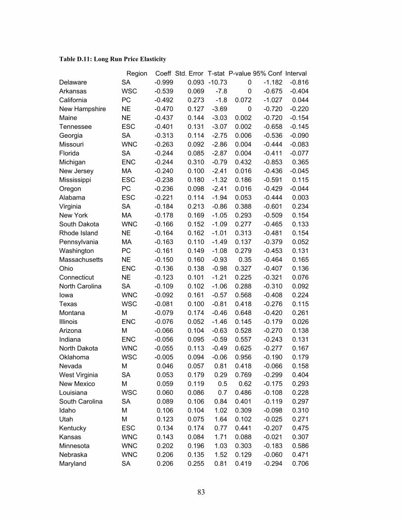
83

Table D.11: Long Run Price Elasticity

Region Coeff Std. Error T-stat P-value 95% Conf Interval

Delaware SA -0.999 0.093 -10.73 0 -1.182 -0.816

Arkansas WSC -0.539 0.069 -7.8 0 -0.675 -0.404

California PC -0.492 0.273 -1.8 0.072 -1.027 0.044

New Hampshire NE -0.470 0.127 -3.69 0 -0.720 -0.220

Maine NE -0.437 0.144 -3.03 0.002 -0.720 -0.154

Tennessee ESC -0.401 0.131 -3.07 0.002 -0.658 -0.145

Georgia SA -0.313 0.114 -2.75 0.006 -0.536 -0.090

Missouri WNC -0.263 0.092 -2.86 0.004 -0.444 -0.083

Florida SA -0.244 0.085 -2.87 0.004 -0.411 -0.077

Michigan ENC -0.244 0.310 -0.79 0.432 -0.853 0.365

New Jersey MA -0.240 0.100 -2.41 0.016 -0.436 -0.045

Mississippi ESC -0.238 0.180 -1.32 0.186 -0.591 0.115

Oregon PC -0.236 0.098 -2.41 0.016 -0.429 -0.044

Alabama ESC -0.221 0.114 -1.94 0.053 -0.444 0.003

Virginia SA -0.184 0.213 -0.86 0.388 -0.601 0.234

New York MA -0.178 0.169 -1.05 0.293 -0.509 0.154

South Dakota WNC -0.166 0.152 -1.09 0.277 -0.465 0.133

Rhode Island NE -0.164 0.162 -1.01 0.313 -0.481 0.154

Pennsylvania MA -0.163 0.110 -1.49 0.137 -0.379 0.052

Washington PC -0.161 0.149 -1.08 0.279 -0.453 0.131

Massachusetts NE -0.150 0.160 -0.93 0.35 -0.464 0.165

Ohio ENC -0.136 0.138 -0.98 0.327 -0.407 0.136

Connecticut NE -0.123 0.101 -1.21 0.225 -0.321 0.076

North Carolina SA -0.109 0.102 -1.06 0.288 -0.310 0.092

Iowa WNC -0.092 0.161 -0.57 0.568 -0.408 0.224

Texas WSC -0.081 0.100 -0.81 0.418 -0.276 0.115

Montana M -0.079 0.174 -0.46 0.648 -0.420 0.261

Illinois ENC -0.076 0.052 -1.46 0.145 -0.179 0.026

Arizona M -0.066 0.104 -0.63 0.528 -0.270 0.138

Indiana ENC -0.056 0.095 -0.59 0.557 -0.243 0.131

North Dakota WNC -0.055 0.113 -0.49 0.625 -0.277 0.167

Oklahoma WSC -0.005 0.094 -0.06 0.956 -0.190 0.179

Nevada M 0.046 0.057 0.81 0.418 -0.066 0.158

West Virginia SA 0.053 0.179 0.29 0.769 -0.299 0.404

New Mexico M 0.059 0.119 0.5 0.62 -0.175 0.293

Louisiana WSC 0.060 0.086 0.7 0.486 -0.108 0.228

South Carolina SA 0.089 0.106 0.84 0.401 -0.119 0.297

Idaho M 0.106 0.104 1.02 0.309 -0.098 0.310

Utah M 0.123 0.075 1.64 0.102 -0.025 0.271

Kentucky ESC 0.134 0.174 0.77 0.441 -0.207 0.475

Kansas WNC 0.143 0.084 1.71 0.088 -0.021 0.307

Minnesota WNC 0.202 0.196 1.03 0.303 -0.183 0.586

Nebraska WNC 0.206 0.135 1.52 0.129 -0.060 0.471

Maryland SA 0.206 0.255 0.81 0.419 -0.294 0.706

84

Vermont NE 0.281 0.580 0.48 0.629 -0.857 1.419

Wyoming M 0.296 0.127 2.33 0.02 0.047 0.545

Wisconsin ENC 0.302 0.183 1.65 0.099 -0.057 0.661

Colorado M 0.666 0.105 6.36 0 0.461 0.872

The long run elasticity estimates show greater variability. Only 12 states have

statistically significant estimates and two of those are positive. Similar to the other

markets, long run price elasticities are generally greater than the short run estimates.

We tested for first-order autocorrelation in the state-level residential electricity model and

found it does not appear to affect the error term. The estimate of was -0.004 with a t-

statistic of -0.89. The results indicate that autocorrelation does not affect consistency of

estimates on the lagged demand term and that inference based on the existing standard

errors is valid.

Commercial Electricity

Table D.12: Short-run elasticity estimates for commercial electricity

Short Run Commercial Electricity

Coef. Std. Err. t P>|t| [95% Conf. Interval]

Tennessee -3.363 2.314 -1.45 0.147 -7.90 1.18

Maryland -1.086 0.946 -1.15 0.251 -2.94 0.77

Nevada -1.016 0.668 -1.52 0.129 -2.33 0.30

Michigan -0.948 0.583 -1.63 0.105 -2.09 0.20

Vermont -0.805 0.212 -3.79 0 -1.22 -0.39

Alabama -0.656 0.288 -2.28 0.023 -1.22 -0.09

South Carolina -0.506 0.195 -2.59 0.01 -0.89 -0.12

Oregon -0.477 0.103 -4.62 0 -0.68 -0.27

Illinois -0.450 0.144 -3.13 0.002 -0.73 -0.17

Montana -0.425 0.515 -0.83 0.409 -1.44 0.59

Rhode Island -0.400 0.107 -3.75 0 -0.61 -0.19

Idaho -0.337 0.282 -1.2 0.232 -0.89 0.22

Washington -0.326 0.255 -1.28 0.201 -0.83 0.17

Massachusetts -0.311 0.099 -3.15 0.002 -0.50 -0.12

New Jersey -0.310 0.109 -2.85 0.004 -0.52 -0.10

Iowa -0.309 0.183 -1.69 0.092 -0.67 0.05

Maine -0.307 0.106 -2.9 0.004 -0.52 -0.10

Texas -0.281 0.112 -2.51 0.012 -0.50 -0.06

Arizona -0.246 0.193 -1.27 0.203 -0.63 0.13

Kansas -0.237 0.113 -2.1 0.036 -0.46 -0.02

Ohio -0.220 0.215 -1.02 0.306 -0.64 0.20

California -0.201 0.123 -1.63 0.104 -0.44 0.04

Connecticut -0.192 0.114 -1.69 0.092 -0.42 0.03

85

Virginia -0.192 0.138 -1.39 0.164 -0.46 0.08

Delaware -0.186 0.163 -1.14 0.256 -0.51 0.14

New Mexico -0.183 0.158 -1.16 0.246 -0.49 0.13

Minnesota -0.173 0.183 -0.95 0.344 -0.53 0.19

Mississippi -0.165 0.224 -0.74 0.462 -0.60 0.27

West Virginia -0.155 0.120 -1.29 0.197 -0.39 0.08

Utah -0.152 0.140 -1.08 0.279 -0.43 0.12

New York -0.150 0.086 -1.75 0.081 -0.32 0.02

Oklahoma -0.108 0.153 -0.7 0.482 -0.41 0.19

Arkansas -0.108 0.153 -0.7 0.481 -0.41 0.19

Louisiana -0.098 0.119 -0.83 0.408 -0.33 0.13

Pennsylvania -0.091 0.073 -1.24 0.216 -0.23 0.05

Florida -0.070 0.121 -0.58 0.561 -0.31 0.17

North Dakota -0.055 0.453 -0.12 0.903 -0.94 0.83

Kentucky -0.053 0.122 -0.44 0.664 -0.29 0.19

Wisconsin -0.033 0.199 -0.17 0.868 -0.42 0.36

North Carolina -0.028 0.106 -0.26 0.793 -0.24 0.18

Missouri -0.022 0.136 -0.16 0.872 -0.29 0.25

Colorado 0.016 0.140 0.12 0.907 -0.26 0.29

Wyoming 0.042 0.132 0.32 0.749 -0.22 0.30

Indiana 0.102 0.174 0.59 0.556 -0.24 0.44

New Hampshire 0.146 0.341 0.43 0.669 -0.52 0.81

Nebraska 0.172 0.157 1.1 0.273 -0.14 0.48

Georgia 0.219 0.117 1.88 0.061 -0.01 0.45

South Dakota 0.335 0.581 0.58 0.564 -0.80 1.48

The state-level estimates lack precision. In comparison to the residential data, the

commercial electricity quantity data have much greater variability, which results in less

precise estimates for price elasticity. As a result, only nine states have statistically

significant results. A data error appears to cause the large estimate for Tennessee. This

data problem was discussed in the regional level section.

The estimates are distributed more evenly throughout the range compared to residential

electricity. There are also fewer positive estimates and none of the positive estimates are

significant.

Table D.13: Long Run Commercial Electricity Elasticity Estimates

Coef. Std. Err. t P>|t| [95% Conf. Interval]

Tennessee -10.338 4.001 -2.58 0.01 -18.19 -2.48

Maryland -7.467 3.332 -2.24 0.025 -14.01 -0.93

Alabama -4.892 4.255 -1.15 0.251 -13.24 3.46

Nevada -1.730 0.859 -2.01 0.044 -3.42 -0.04

Michigan -1.496 0.537 -2.79 0.005 -2.55 -0.44

Rhode Island -1.315 1.232 -1.07 0.286 -3.73 1.10

Ohio -1.243 1.500 -0.83 0.407 -4.19 1.70

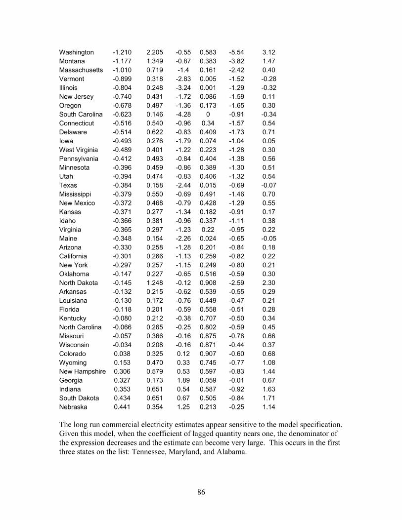
86

Washington -1.210 2.205 -0.55 0.583 -5.54 3.12

Montana -1.177 1.349 -0.87 0.383 -3.82 1.47

Massachusetts -1.010 0.719 -1.4 0.161 -2.42 0.40

Vermont -0.899 0.318 -2.83 0.005 -1.52 -0.28

Illinois -0.804 0.248 -3.24 0.001 -1.29 -0.32

New Jersey -0.740 0.431 -1.72 0.086 -1.59 0.11

Oregon -0.678 0.497 -1.36 0.173 -1.65 0.30

South Carolina -0.623 0.146 -4.28 0 -0.91 -0.34

Connecticut -0.516 0.540 -0.96 0.34 -1.57 0.54

Delaware -0.514 0.622 -0.83 0.409 -1.73 0.71

Iowa -0.493 0.276 -1.79 0.074 -1.04 0.05

West Virginia -0.489 0.401 -1.22 0.223 -1.28 0.30

Pennsylvania -0.412 0.493 -0.84 0.404 -1.38 0.56

Minnesota -0.396 0.459 -0.86 0.389 -1.30 0.51

Utah -0.394 0.474 -0.83 0.406 -1.32 0.54

Texas -0.384 0.158 -2.44 0.015 -0.69 -0.07

Mississippi -0.379 0.550 -0.69 0.491 -1.46 0.70

New Mexico -0.372 0.468 -0.79 0.428 -1.29 0.55

Kansas -0.371 0.277 -1.34 0.182 -0.91 0.17

Idaho -0.366 0.381 -0.96 0.337 -1.11 0.38

Virginia -0.365 0.297 -1.23 0.22 -0.95 0.22

Maine -0.348 0.154 -2.26 0.024 -0.65 -0.05

Arizona -0.330 0.258 -1.28 0.201 -0.84 0.18

California -0.301 0.266 -1.13 0.259 -0.82 0.22

New York -0.297 0.257 -1.15 0.249 -0.80 0.21

Oklahoma -0.147 0.227 -0.65 0.516 -0.59 0.30

North Dakota -0.145 1.248 -0.12 0.908 -2.59 2.30

Arkansas -0.132 0.215 -0.62 0.539 -0.55 0.29

Louisiana -0.130 0.172 -0.76 0.449 -0.47 0.21

Florida -0.118 0.201 -0.59 0.558 -0.51 0.28

Kentucky -0.080 0.212 -0.38 0.707 -0.50 0.34

North Carolina -0.066 0.265 -0.25 0.802 -0.59 0.45

Missouri -0.057 0.366 -0.16 0.875 -0.78 0.66

Wisconsin -0.034 0.208 -0.16 0.871 -0.44 0.37

Colorado 0.038 0.325 0.12 0.907 -0.60 0.68

Wyoming 0.153 0.470 0.33 0.745 -0.77 1.08

New Hampshire 0.306 0.579 0.53 0.597 -0.83 1.44

Georgia 0.327 0.173 1.89 0.059 -0.01 0.67

Indiana 0.353 0.651 0.54 0.587 -0.92 1.63

South Dakota 0.434 0.651 0.67 0.505 -0.84 1.71

Nebraska 0.441 0.354 1.25 0.213 -0.25 1.14

The long run commercial electricity estimates appear sensitive to the model specification.

Given this model, when the coefficient of lagged quantity nears one, the denominator of

the expression decreases and the estimate can become very large. This occurs in the first

three states on the list: Tennessee, Maryland, and Alabama.

87

The remaining estimates are generally larger than the short run estimates. The states also

remain in relatively similar positions to the short run estimates.

We tested for first-order autocorrelation in the state-level commercial electricity model

and found it does not appear to affect the error term. The estimate of was 0.018 with a

t-statistic of 0.50. The results indicate that autocorrelation does not affect consistency of

estimates on the lagged demand term and that inference based on the existing standard

errors is valid.

Natural Gas

Table D.14: Regression results for short run residential natural gas elasticity.

Short Run Natural Gas

Coef. Std. Err. t P>|t| [95% Conf. Interval]

Maine -0.745 0.467 -1.59 0.111 -1.662 0.172

Vermont -0.281 0.084 -3.35 0.001 -0.445 -0.117

Illinois -0.229 0.084 -2.72 0.007 -0.394 -0.064

New Hampshire -0.225 0.093 -2.41 0.016 -0.408 -0.042

Montana -0.217 0.079 -2.75 0.006 -0.372 -0.062

South Carolina -0.202 0.141 -1.43 0.154 -0.479 0.076

New Mexico -0.190 0.111 -1.71 0.088 -0.408 0.028

Virginia -0.189 0.104 -1.81 0.07 -0.393 0.015

West Virginia -0.184 0.083 -2.22 0.027 -0.347 -0.021

North Dakota -0.183 0.063 -2.88 0.004 -0.308 -0.059

Alabama -0.170 0.103 -1.64 0.101 -0.372 0.033

Kansas -0.167 0.071 -2.37 0.018 -0.305 -0.028

Washington -0.166 0.109 -1.53 0.125 -0.380 0.047

Arkansas -0.151 0.080 -1.89 0.059 -0.308 0.006

North Carolina -0.149 0.102 -1.46 0.145 -0.350 0.052

Missouri -0.143 0.068 -2.11 0.035 -0.276 -0.010

Indiana -0.139 0.063 -2.21 0.027 -0.263 -0.015

Kentucky -0.137 0.059 -2.31 0.021 -0.253 -0.021

Ohio -0.127 0.076 -1.68 0.093 -0.276 0.021

Pennsylvania -0.117 0.089 -1.31 0.19 -0.291 0.058

South Dakota -0.112 0.077 -1.46 0.144 -0.263 0.039

Tennessee -0.110 0.101 -1.09 0.277 -0.308 0.088

Maryland -0.106 0.109 -0.97 0.331 -0.319 0.108

Colorado -0.102 0.069 -1.48 0.14 -0.237 0.033

Minnesota -0.100 0.066 -1.52 0.129 -0.229 0.029

California -0.098 0.119 -0.82 0.41 -0.332 0.135

Iowa -0.098 0.090 -1.09 0.278 -0.275 0.079

Wisconsin -0.098 0.066 -1.49 0.138 -0.227 0.031

Rhode Island -0.085 0.122 -0.7 0.485 -0.323 0.154

Idaho -0.074 0.076 -0.98 0.329 -0.223 0.075

Mississippi -0.061 0.080 -0.76 0.448 -0.217 0.096

Michigan -0.047 0.083 -0.57 0.57 -0.209 0.115

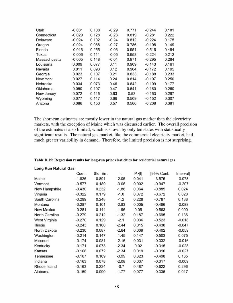
88

Utah -0.031 0.108 -0.29 0.771 -0.244 0.181

Connecticut -0.029 0.128 -0.23 0.819 -0.281 0.222

Delaware -0.024 0.102 -0.24 0.812 -0.224 0.175

Oregon -0.024 0.088 -0.27 0.786 -0.198 0.149

Florida -0.016 0.255 -0.06 0.951 -0.516 0.484

Texas -0.006 0.111 -0.05 0.958 -0.224 0.212

Massachusetts -0.005 0.148 -0.04 0.971 -0.295 0.284

Louisiana 0.009 0.077 0.11 0.909 -0.143 0.161

Nevada 0.011 0.093 0.12 0.904 -0.172 0.195

Georgia 0.023 0.107 0.21 0.833 -0.188 0.233

New York 0.027 0.114 0.24 0.814 -0.197 0.250

Nebraska 0.034 0.073 0.46 0.642 -0.109 0.177

Oklahoma 0.050 0.107 0.47 0.641 -0.160 0.260

New Jersey 0.072 0.115 0.63 0.53 -0.153 0.297

Wyoming 0.077 0.117 0.66 0.509 -0.152 0.307

Arizona 0.086 0.150 0.57 0.566 -0.208 0.381

The short-run estimates are mostly lower in the natural gas market than the electricity

markets, with the exception of Maine which was discussed earlier. The overall precision

of the estimates is also limited, which is shown by only ten states with statistically

significant results. The natural gas market, like the commercial electricity market, had

much greater variability in demand. Therefore, the limited precision is not surprising.

Table D.15: Regression results for long-run price elasticities for residential natural gas

Long Run Natural Gas

Coef. Std. Err. t P>|t| [95% Conf. Interval]

Maine -1.826 0.891 -2.05 0.041 -3.575 -0.078

Vermont -0.577 0.189 -3.06 0.002 -0.947 -0.207

New Hampshire -0.430 0.232 -1.86 0.064 -0.885 0.024

Virginia -0.322 0.179 -1.8 0.072 -0.672 0.028

South Carolina -0.299 0.248 -1.2 0.228 -0.787 0.188

Montana -0.287 0.101 -2.83 0.005 -0.486 -0.088

New Mexico -0.281 0.144 -1.96 0.05 -0.563 0.000

North Carolina -0.279 0.212 -1.32 0.187 -0.695 0.136

West Virginia -0.270 0.129 -2.1 0.036 -0.523 -0.018

Illinois -0.243 0.100 -2.44 0.015 -0.438 -0.047

North Dakota -0.230 0.087 -2.64 0.009 -0.402 -0.059

Washington -0.214 0.147 -1.45 0.147 -0.503 0.075

Missouri -0.174 0.081 -2.16 0.031 -0.332 -0.016

Kentucky -0.171 0.073 -2.34 0.02 -0.315 -0.028

Kansas -0.168 0.072 -2.34 0.019 -0.310 -0.027

Tennessee -0.167 0.169 -0.99 0.323 -0.498 0.165

Indiana -0.163 0.078 -2.08 0.037 -0.317 -0.009

Rhode Island -0.163 0.234 -0.7 0.487 -0.622 0.296

Alabama -0.159 0.090 -1.77 0.077 -0.336 0.017

89

South Dakota -0.142 0.107 -1.33 0.183 -0.352 0.067

Arkansas -0.141 0.075 -1.87 0.062 -0.289 0.007

Maryland -0.134 0.136 -0.99 0.323 -0.400 0.132

Minnesota -0.133 0.088 -1.5 0.134 -0.306 0.041

California -0.132 0.166 -0.8 0.425 -0.458 0.193

Ohio -0.132 0.081 -1.64 0.101 -0.291 0.026

Pennsylvania -0.124 0.098 -1.27 0.205 -0.315 0.068

Colorado -0.122 0.075 -1.63 0.104 -0.270 0.025

Iowa -0.114 0.109 -1.04 0.296 -0.329 0.100

Wisconsin -0.110 0.075 -1.46 0.145 -0.257 0.038

Idaho -0.104 0.112 -0.94 0.35 -0.323 0.115

Mississippi -0.079 0.110 -0.72 0.471 -0.295 0.136

Michigan -0.075 0.131 -0.57 0.567 -0.333 0.182

Utah -0.061 0.213 -0.29 0.776 -0.478 0.357

Connecticut -0.042 0.184 -0.23 0.818 -0.402 0.318

Delaware -0.036 0.153 -0.24 0.813 -0.337 0.264

Oregon -0.028 0.104 -0.27 0.788 -0.232 0.176

Florida -0.020 0.317 -0.06 0.951 -0.642 0.603

Massachusetts -0.009 0.256 -0.04 0.971 -0.512 0.494

Texas -0.008 0.159 -0.05 0.958 -0.320 0.303

Louisiana 0.011 0.093 0.11 0.909 -0.171 0.193

Nevada 0.021 0.175 0.12 0.905 -0.323 0.365

Georgia 0.022 0.105 0.21 0.834 -0.185 0.229

New York 0.029 0.124 0.24 0.812 -0.213 0.272

Nebraska 0.038 0.081 0.47 0.64 -0.121 0.197

Oklahoma 0.056 0.120 0.47 0.641 -0.179 0.291

New Jersey 0.082 0.129 0.63 0.528 -0.172 0.335

Wyoming 0.092 0.127 0.73 0.465 -0.156 0.341

Arizona 0.119 0.220 0.54 0.588 -0.312 0.550

Similar to other markets, the long-run estimates are generally larger than the short run

estimates. The precision of these estimates is also limited, which is shown by the large

standard errors and that only ten states have statistically significant estimates. The

natural gas market also had much greater variation in prices and quantity during this

period, which appears to affect the results at this level of aggregation. With the exception

of Maine, the range of estimates is smaller than the electricity markets, which

corresponds to the generally smaller (in absolute magnitude) values of the estimates when

compared to the other markets.

We tested for first-order autocorrelation in the state-level residential natural gas model

and found it does not appear to affect the error term. The estimate of was -0.12 with a

t-statistic of -1.75. The results indicate that autocorrelation does not affect consistency of

estimates on the lagged demand term and that inference based on the existing standard

errors is valid.

90

Utility-level results

Table D.16: Short run elasticity estimates for residential electricity at the utility level

UtilityNumber region Coef. Std. Err. t P>|t|

[95% Conf. Interval]

182 ENC -1.563 0.472 -3.31 0.001 -2.490 -0.637

208 ENC -1.081 0.633 -1.71 0.088 -2.323 0.160

186 ENC -1.061 0.521 -2.04 0.042 -2.082 -0.039

191 ENC -0.697 0.275 -2.54 0.011 -1.237 -0.158

18 ENC -0.584 0.279 -2.1 0.036 -1.13 -0.04

75 ENC -0.480 0.498 -0.96 0.335 -1.46 0.50

134 ENC -0.392 0.257 -1.53 0.127 -0.896 0.112

153 ENC -0.314 0.238 -1.32 0.188 -0.781 0.154

35 ENC -0.250 0.160 -1.57 0.118 -0.56 0.06

73 ENC -0.243 0.135 -1.8 0.072 -0.51 0.02

177 ENC -0.217 0.622 -0.35 0.728 -1.438 1.004

67 ENC -0.167 0.245 -0.68 0.495 -0.65 0.31

41 ENC -0.150 0.353 -0.43 0.671 -0.84 0.54

44 ENC -0.137 0.291 -0.47 0.637 -0.71 0.43

17 ENC -0.131 0.469 -0.28 0.78 -1.05 0.79

76 ENC -0.105 0.337 -0.31 0.756 -0.77 0.56

38 ENC -0.097 0.427 -0.23 0.82 -0.93 0.74

26 ENC -0.091 0.359 -0.25 0.8 -0.80 0.61

96 ENC -0.082 0.331 -0.25 0.803 -0.73 0.57

105 ENC -0.070 0.175 -0.4 0.689 -0.41 0.27

28 ENC -0.045 0.399 -0.11 0.909 -0.83 0.74

33 ENC -0.033 0.320 -0.1 0.917 -0.66 0.59

206 ENC -0.004 0.517 -0.01 0.994 -1.019 1.011

133 ENC 0.024 0.490 0.05 0.96 -0.936 0.985

207 ENC 0.109 0.355 0.31 0.758 -0.587 0.806

129 ENC 0.211 0.563 0.37 0.708 -0.894 1.315

130 ENC 0.952 1.475 0.65 0.519 -1.941 3.845

103 ESC -1.514 0.410 -3.69 0 -2.32 -0.71

113 ESC -1.222 0.397 -3.08 0.002 -2.00 -0.44

47 ESC -1.126 0.675 -1.67 0.096 -2.45 0.20

120 ESC -1.064 0.625 -1.7 0.089 -2.291 0.163

30 ESC -1.046 0.689 -1.52 0.129 -2.40 0.31

198 ESC -0.958 0.414 -2.32 0.021 -1.770 -0.147

40 ESC -0.884 0.857 -1.03 0.302 -2.56 0.80

110 ESC -0.766 0.389 -1.97 0.049 -1.53 0.00

92 ESC -0.680 0.598 -1.14 0.256 -1.85 0.49

86 ESC -0.528 0.394 -1.34 0.181 -1.30 0.25

179 ESC -0.499 0.230 -2.17 0.03 -0.950 -0.048

69 ESC -0.486 0.592 -0.82 0.411 -1.65 0.67

98 ESC -0.439 0.835 -0.53 0.599 -2.08 1.20

193 ESC -0.299 0.386 -0.77 0.439 -1.055 0.458

172 ESC -0.297 0.276 -1.07 0.283 -0.839 0.245

1 ESC -0.200 0.522 -0.38 0.701 -1.22 0.82

23 ESC -0.192 0.521 -0.37 0.713 -1.21 0.83

91

107 ESC -0.178 0.548 -0.32 0.746 -1.25 0.90

93 ESC -0.088 0.226 -0.39 0.699 -0.53 0.36

210 ESC -0.018 0.801 -0.02 0.982 -1.589 1.552

57 ESC 0.148 0.745 0.2 0.843 -1.31 1.61

91 ESC 0.317 0.338 0.94 0.348 -0.35 0.98

112 ESC 0.402 0.612 0.66 0.511 -0.80 1.60

200 ESC 1.389 0.305 4.55 0 0.790 1.987

211 M -1.206 0.394 -3.06 0.002 -1.979 -0.433

94 M -1.084 0.629 -1.72 0.085 -2.32 0.15

140 M -0.980 0.401 -2.45 0.015 -1.767 -0.194

155 M -0.696 0.248 -2.81 0.005 -1.183 -0.210

171 M -0.694 0.586 -1.18 0.237 -1.844 0.456

184 M -0.663 0.607 -1.09 0.274 -1.854 0.527

164 M -0.547 0.403 -1.36 0.174 -1.338 0.243

151 M -0.368 1.027 -0.36 0.72 -2.382 1.647

53 M -0.325 0.725 -0.45 0.655 -1.75 1.10

122 M -0.262 0.075 -3.51 0 -0.409 -0.116

152 M -0.260 0.396 -0.66 0.512 -1.036 0.516

32 M -0.233 0.649 -0.36 0.72 -1.51 1.04

5 M -0.221 0.372 -0.59 0.552 -0.95 0.51

118 M -0.096 0.187 -0.51 0.61 -0.463 0.272

196 M -0.061 0.305 -0.2 0.842 -0.660 0.538

25 M -0.014 0.253 -0.06 0.955 -0.51 0.48

104 M -0.001 0.283 0 0.996 -0.56 0.55

71 M 0.467 0.298 1.57 0.117 -0.12 1.05

202 MA -0.800 0.429 -1.87 0.062 -1.641 0.041

109 MA -0.792 0.625 -1.27 0.205 -2.02 0.43

37 MA -0.712 0.600 -1.19 0.235 -1.89 0.46

100 MA -0.639 0.418 -1.53 0.126 -1.46 0.18

160 MA -0.417 0.383 -1.09 0.277 -1.169 0.336

125 MA -0.345 0.321 -1.07 0.284 -0.975 0.286

147 MA -0.341 0.284 -1.2 0.23 -0.897 0.216

145 MA -0.308 0.477 -0.65 0.518 -1.244 0.627

213 MA -0.230 0.301 -0.76 0.446 -0.821 0.361

85 MA -0.177 0.364 -0.49 0.626 -0.89 0.54

157 MA -0.117 0.475 -0.25 0.805 -1.050 0.815

49 MA -0.089 0.240 -0.37 0.711 -0.56 0.38

161 MA -0.003 0.492 -0.01 0.996 -0.967 0.962

16 MA 0.077 0.478 0.16 0.872 -0.86 1.02

137 MA 0.099 0.329 0.3 0.763 -0.546 0.744

146 MA 0.125 0.146 0.86 0.39 -0.161 0.412

7 MA 0.171 0.180 0.95 0.341 -0.18 0.52

144 MA 0.302 0.323 0.94 0.35 -0.332 0.936

126 MA 0.350 0.296 1.18 0.238 -0.231 0.932

20 NE -0.722 0.421 -1.72 0.086 -1.55 0.10

119 NE -0.596 0.569 -1.05 0.296 -1.713 0.521

65 NE -0.546 0.149 -3.65 0 -0.84 -0.25

22 NE -0.391 0.278 -1.41 0.159 -0.94 0.15

123 NE -0.360 0.229 -1.57 0.117 -0.809 0.090

194 NE -0.197 0.535 -0.37 0.712 -1.246 0.851

92

34 NE -0.196 0.212 -0.93 0.355 -0.61 0.22

36 NE -0.154 0.348 -0.44 0.659 -0.84 0.53

14 NE -0.091 0.254 -0.36 0.721 -0.59 0.41

46 NE -0.019 0.272 -0.07 0.946 -0.55 0.52

4 NE 0.063 0.416 0.15 0.88 -0.75 0.88

154 NE 0.072 0.723 0.1 0.92 -1.346 1.491

10 NE 0.191 0.333 0.57 0.566 -0.46 0.84

204 NE 0.197 0.400 0.49 0.622 -0.587 0.981

106 NE 0.849 0.908 0.93 0.35 -0.93 2.63

139 PC -1.215 0.094 -12.96 0 -1.399 -1.031

24 PC -0.961 0.035 -27.6 0 -1.03 -0.89

2 PC -0.770 0.144 -5.35 0 -1.05 -0.49

173 PC -0.595 0.568 -1.05 0.295 -1.711 0.520

158 PC -0.488 0.486 -1 0.315 -1.440 0.465

101 PC -0.471 0.269 -1.75 0.081 -1.00 0.06

64 PC -0.444 0.324 -1.37 0.171 -1.08 0.19

166 PC -0.430 0.366 -1.18 0.24 -1.147 0.287

176 PC -0.279 0.365 -0.76 0.444 -0.995 0.437

39 PC -0.219 0.228 -0.96 0.336 -0.67 0.23

188 PC -0.156 0.379 -0.41 0.682 -0.899 0.588

27 PC -0.119 0.431 -0.28 0.783 -0.96 0.73

142 PC -0.119 0.335 -0.35 0.724 -0.776 0.539

170 PC 0.014 0.377 0.04 0.971 -0.726 0.754

74 PC 0.068 0.303 0.23 0.822 -0.53 0.66

163 PC 0.144 0.511 0.28 0.778 -0.859 1.147

201 PC 0.279 0.552 0.5 0.614 -0.805 1.362

11 PC 0.324 0.181 1.79 0.073 -0.03 0.68

159 PC 0.404 0.548 0.74 0.461 -0.671 1.479

115 PC 0.475 0.421 1.13 0.26 -0.35 1.30

148 PC 0.670 0.402 1.66 0.096 -0.120 1.459

52 PC 0.756 0.515 1.47 0.142 -0.25 1.77

197 SA -1.477 0.743 -1.99 0.047 -2.935 -0.020

178 SA -1.434 0.542 -2.65 0.008 -2.497 -0.371

29 SA -1.299 0.474 -2.74 0.006 -2.23 -0.37

63 SA -1.232 0.725 -1.7 0.09 -2.65 0.19

199 SA -1.150 0.635 -1.81 0.07 -2.396 0.096

187 SA -1.087 0.525 -2.07 0.039 -2.118 -0.056

95 SA -1.073 0.621 -1.73 0.085 -2.29 0.15

31 SA -1.038 0.238 -4.36 0 -1.50 -0.57

97 SA -1.032 0.621 -1.66 0.097 -2.25 0.19

127 SA -0.890 0.660 -1.35 0.178 -2.186 0.405

169 SA -0.884 0.366 -2.42 0.016 -1.602 -0.167

84 SA -0.878 0.566 -1.55 0.121 -1.99 0.23

168 SA -0.854 0.290 -2.94 0.003 -1.423 -0.284

189 SA -0.827 0.607 -1.36 0.173 -2.018 0.363

83 SA -0.814 0.306 -2.66 0.008 -1.41 -0.21

15 SA -0.734 0.583 -1.26 0.208 -1.88 0.41

128 SA -0.686 0.297 -2.31 0.021 -1.270 -0.103

60 SA -0.678 0.368 -1.84 0.066 -1.40 0.05

48 SA -0.542 0.673 -0.8 0.421 -1.86 0.78

93

72 SA -0.540 0.504 -1.07 0.284 -1.53 0.45

116 SA -0.472 0.298 -1.58 0.113 -1.06 0.11

190 SA -0.458 0.501 -0.91 0.361 -1.441 0.525

62 SA -0.447 0.320 -1.4 0.162 -1.07 0.18

174 SA -0.438 0.541 -0.81 0.418 -1.498 0.623

66 SA -0.304 0.334 -0.91 0.363 -0.96 0.35

58 SA -0.299 0.373 -0.8 0.422 -1.03 0.43

56 SA -0.272 0.366 -0.74 0.458 -0.99 0.45

82 SA -0.243 0.354 -0.69 0.492 -0.94 0.45

54 SA -0.195 0.388 -0.5 0.614 -0.96 0.57

141 SA -0.164 0.102 -1.61 0.108 -0.363 0.036

214 SA -0.160 0.388 -0.41 0.681 -0.921 0.602

12 SA -0.129 0.212 -0.61 0.544 -0.55 0.29

9 SA -0.124 0.426 -0.29 0.772 -0.96 0.71

175 SA -0.123 0.273 -0.45 0.651 -0.658 0.412

149 SA -0.004 0.431 -0.01 0.993 -0.850 0.842

209 SA 0.004 0.473 0.01 0.994 -0.925 0.933

43 SA 0.038 0.405 0.09 0.925 -0.76 0.83

59 SA 0.041 0.448 0.09 0.928 -0.84 0.92

205 SA 0.234 0.383 0.61 0.541 -0.517 0.986

42 SA 0.241 1.088 0.22 0.825 -1.89 2.38

162 SA 0.488 0.374 1.31 0.192 -0.245 1.221

78 WNC -1.746 1.057 -1.65 0.099 -3.82 0.33

192 WNC -1.127 0.243 -4.64 0 -1.604 -0.651

131 WNC -0.654 0.332 -1.97 0.049 -1.307 -0.002

88 WNC -0.622 0.261 -2.39 0.017 -1.13 -0.11

90 WNC -0.615 0.364 -1.69 0.091 -1.33 0.10

150 WNC -0.552 0.188 -2.94 0.003 -0.920 -0.184

114 WNC -0.495 0.749 -0.66 0.509 -1.96 0.97

132 WNC -0.476 0.447 -1.06 0.287 -1.353 0.401

77 WNC -0.471 0.336 -1.4 0.162 -1.13 0.19

183 WNC -0.463 0.115 -4.02 0 -0.688 -0.237

111 WNC -0.440 0.303 -1.45 0.146 -1.03 0.15

136 WNC -0.425 0.373 -1.14 0.255 -1.157 0.308

89 WNC -0.352 0.221 -1.59 0.111 -0.79 0.08

79 WNC -0.200 0.522 -0.38 0.701 -1.22 0.82

80 WNC -0.200 0.522 -0.38 0.701 -1.22 0.82

81 WNC -0.200 0.522 -0.38 0.701 -1.22 0.82

3 WNC -0.190 0.411 -0.46 0.643 -1.00 0.62

108 WNC -0.153 0.427 -0.36 0.719 -0.99 0.68

87 WNC -0.124 0.404 -0.31 0.758 -0.92 0.67

195 WNC -0.070 0.455 -0.15 0.878 -0.962 0.822

138 WNC -0.052 0.419 -0.13 0.901 -0.874 0.769

185 WNC 0.041 0.406 0.1 0.921 -0.757 0.838

121 WNC 0.179 0.268 0.67 0.504 -0.346 0.704

99 WNC 0.489 0.717 0.68 0.496 -0.92 1.90

212 WNC 1.109 0.779 1.42 0.155 -0.420 2.638

51 WNC 1.404 0.422 3.32 0.001 0.58 2.23

135 WSC -1.226 0.591 -2.07 0.038 -2.385 -0.067

6 WSC -0.917 0.283 -3.24 0.001 -1.47 -0.36

94

215 WSC -0.632 0.354 -1.78 0.075 -1.326 0.063

102 WSC -0.615 0.344 -1.79 0.074 -1.29 0.06

124 WSC -0.613 0.254 -2.42 0.016 -1.111 -0.115

13 WSC -0.517 0.726 -0.71 0.476 -1.94 0.91

55 WSC -0.485 0.335 -1.45 0.148 -1.14 0.17

167 WSC -0.484 0.437 -1.11 0.268 -1.340 0.373

45 WSC -0.464 0.265 -1.75 0.08 -0.98 0.06

19 WSC -0.450 0.448 -1 0.315 -1.33 0.43

181 WSC -0.318 0.331 -0.96 0.338 -0.968 0.332

156 WSC -0.286 0.440 -0.65 0.516 -1.150 0.578

165 WSC -0.272 0.404 -0.67 0.502 -1.065 0.522

21 WSC -0.154 0.292 -0.53 0.597 -0.73 0.42

68 WSC -0.108 0.234 -0.46 0.646 -0.57 0.35

70 WSC -0.091 0.508 -0.18 0.858 -1.09 0.91

180 WSC 0.023 0.587 0.04 0.969 -1.129 1.174

8 WSC 0.066 0.406 0.16 0.872 -0.73 0.86

203 WSC 0.447 0.205 2.18 0.03 0.044 0.851

61 WSC 0.452 0.317 1.43 0.154 -0.17 1.07

50 WSC 0.486 0.427 1.14 0.255 -0.35 1.32

143 WSC 0.614 0.440 1.39 0.163 -0.250 1.477

The utility results also have a wide range of price elasticity estimates. The minimum

value is –1.75 and the maximum is 1.40. In general, the estimates are representative of

the results from the state-level analysis in residential electricity. Most estimates are

negative and in the inelastic range. Some are positive in each region. Overall, these

results suffer from a lack of precision also. Only about 17% of the utilities in the sample

were statistically significant. Some of this variation in the estimates may be explained by

the large differences in the size of utilities.

We tested for first-order autocorrelation in the error term and the results indicate it may

be present. The estimate of for the utility-level model was -0.32 with a t-statistic of

-3.27. The results suggest first-order autocorrelation in the error term and we, therefore,

ran the model to account for an AR(1) structure in the error term.

Results from Energy Use Trend Analysis

The trend analysis fits a linear trend to the variable of interest. Many of the trends in the

data were linear and the model fit well. In some cases, particularly the natural gas

market, the trends were not linear and the model had a poorer fit.

This section will now display the trend analysis results first for the region level and then

at the state level.

95

Regional-Level Results

The model has the form:

ln yit = + yeart + regioni i + (regioni x yeart) i + it

The model includes an indicator variable for region and an interaction term between

region and year. These terms allow the slope of the trend and y-intercept to vary freely

for each region.

Residential Electricity

Table D.17: Regional trends in residential electricity energy intensity

Coef Std. Err. t P>|t| 95% Conf Interval

South Atlantic 1.94% 0.08% 25.7 0.0 1.79% 2.09%

East South Central 1.79% 0.11% 16.8 0.0 1.59% 2.00%

West South Central 1.59% 0.11% 14.9 0.0 1.38% 1.80%

West North Central 1.45% 0.08% 18.0 0.0 1.29% 1.61%

East North Central 1.40% 0.10% 14.6 0.0 1.21% 1.58%

Mid Atlantic 1.33% 0.12% 10.8 0.0 1.09% 1.57%

New England 0.91% 0.09% 10.4 0.0 0.73% 1.08%

Mountain 0.80% 0.08% 10.6 0.0 0.65% 0.95%

Pacific Coast -0.12% 0.12% -1.0 0.3 -0.36% 0.12%

Intensity is measured as quantity of residential electricity per capita. The table shows per

capita electricity use is growing fastest in the South Atlantic and Central regions. Growth

in per capita electricity use is negligible in the Pacific Coast region.

Table D.18: Regional trends in residential electricity expenditures

Coef Std. Err. t P>|t| 95% Conf Interval

New England 0.717% 0.111% 6.49 0 0.500% 0.934%

Pacific Coast 0.680% 0.156% 4.35 0 0.373% 0.987%

East South Central 0.624% 0.135% 4.61 0 0.358% 0.890%

South Atlantic 0.621% 0.096% 6.48 0 0.433% 0.809%

West South Central 0.518% 0.135% 3.83 0 0.253% 0.784%

Mid Atlantic 0.316% 0.156% 2.02 0.04 0.009% 0.623%

West North Central 0.143% 0.102% 1.4 0.16 -0.058% 0.344%

East North Central 0.122% 0.121% 1.01 0.32 -0.116% 0.359%

Mountain 0.008% 0.096% 0.09 0.93 -0.180% 0.196%

Expenditures are growing fastest in the New England and Pacific Coast regions. Growth

in expenditures is negligible in the Mountain region. Overall, the growth rates are all less

than 1%.

96

Table D.19: Regional trends in residential electricity expenditures as a share of income

Coef Std. Err. t P>|t| 95% Conf Interval

Mid Atlantic -1.99% 0.17% -12.08 0 -2.32% -1.67%

West North Central -1.98% 0.11% -18.32 0 -2.19% -1.77%

East North Central -1.90% 0.13% -14.83 0 -2.15% -1.65%

Mountain -1.83% 0.10% -18.07 0 -2.03% -1.63%

New England -1.82% 0.12% -15.58 0 -2.05% -1.59%

East South Central -1.80% 0.14% -12.57 0 -2.08% -1.52%

South Atlantic -1.71% 0.10% -16.9 0 -1.91% -1.51%

West South Central -1.46% 0.14% -10.24 0 -1.74% -1.18%

Pacific Coast -1.19% 0.17% -7.21 0 -1.51% -0.87%

The trends in expenditures as a share of income show that income growth is faster than

the increase in energy expenditures. Therefore, energy expenditures as a portion of

household budgets is generally decreasing. The regional differences in the rate of

decrease vary by about 1%. Expenditures as a share of income are declining fastest in the

Mid Atlantic at about 2%. Decline is slowest in the Pacific Coast region at

approximately 1%.

Commercial Electricity

Table D.20: Regional trends in commercial energy intensity

Regional commercial energy intensity trends R-square = 0.57

Coef. Std. Err. t P>|t| [95% Conf. Interval]

New England 2.32% 0.20% 11.42 0 1.92% 2.72%

West North Central 2.18% 0.30% 7.15 0 1.58% 2.77%

South Atlantic 1.97% 0.20% 9.9 0 1.58% 2.36%

Mid Atlantic 1.78% 0.25% 7.01 0 1.28% 2.28%

East North Central 1.49% 0.20% 7.58 0 1.10% 1.87%

Mountain 1.48% 0.29% 5.19 0 0.92% 2.04%

West South Central 0.96% 0.25% 3.81 0 0.47% 1.45%

East South Central 0.94% 0.46% 2.04 0.041 0.04% 1.84%

Pacific Coast 0.25% 0.32% 0.8 0.425 -0.37% 0.88%

Intensity is measured as quantity of commercial electricity per unit of commercial

floorspace. The results show statistically significant differences in the annual growth

rates. The Pacific Coast rate is near zero, whereas the annual growth rates are over 2% in

New England and the West North Central. All the trend estimates are statistically

significant, except the Pacific Coast region. However, the model fit is only moderate,

which is shown by the adjusted R-squared of 0.57.

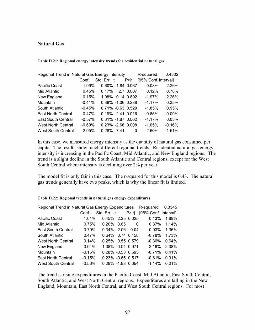
97

Natural Gas

Table D.21: Regional energy intensity trends for residential natural gas

Regional Trend in Natural Gas Energy Intensity R-squared 0.4302

Coef. Std. Err. t P>|t| [95% Conf. Interval]

Pacific Coast 1.09% 0.60% 1.84 0.067 -0.08% 2.26%

Mid Atlantic 0.45% 0.17% 2.7 0.007 0.12% 0.78%

New England 0.15% 1.08% 0.14 0.892 -1.97% 2.26%

Mountain -0.41% 0.39% -1.06 0.288 -1.17% 0.35%

South Atlantic -0.45% 0.71% -0.63 0.529 -1.85% 0.95%

East North Central -0.47% 0.19% -2.41 0.016 -0.85% -0.09%

East South Central -0.57% 0.31% -1.87 0.062 -1.17% 0.03%

West North Central -0.60% 0.23% -2.66 0.008 -1.05% -0.16%

West South Central -2.05% 0.28% -7.41 0 -2.60% -1.51%

In this case, we measured energy intensity as the quantity of natural gas consumed per

capita. The results show much different regional trends. Residential natural gas energy

intensity is increasing in the Pacific Coast, Mid Atlantic, and New England regions. The

trend is a slight decline in the South Atlantic and Central regions, except for the West

South Central where intensity is declining over 2% per year.

The model fit is only fair in this case. The r-squared for this model is 0.43. The natural

gas trends generally have two peaks, which is why the linear fit is limited.

Table D.22: Regional trends in natural gas energy expenditures

Regional Trend in Natural Gas Energy Expenditures R-squared 0.3345

Coef. Std. Err. t P>|t| [95% Conf. Interval]

Pacific Coast 1.01% 0.45% 2.25 0.025 0.13% 1.89%

Mid Atlantic 0.75% 0.20% 3.85 0 0.37% 1.14%

East South Central 0.70% 0.34% 2.06 0.04 0.03% 1.36%

South Atlantic 0.47% 0.64% 0.74 0.458 -0.78% 1.73%

West North Central 0.14% 0.25% 0.55 0.579 -0.36% 0.64%

New England -0.04% 1.08% -0.04 0.971 -2.16% 2.08%

Mountain -0.15% 0.28% -0.53 0.595 -0.71% 0.41%

East North Central -0.15% 0.23% -0.65 0.517 -0.61% 0.31%

West South Central -0.56% 0.29% -1.93 0.054 -1.14% 0.01%

The trend is rising expenditures in the Pacific Coast, Mid Atlantic, East South Central,

South Atlantic, and West North Central regions. Expenditures are falling in the New

England, Mountain, East North Central, and West South Central regions. For most

98

regions, the trend is near or less than 0.5% in absolute magnitude. Therefore, the

estimates show that expenditures are relatively stable for most people.

The model fit is marginal in this case. Natural gas prices had several spikes and dropoffs,

which is a nonlinear pattern. The expenditure data follow the price trend closely.

Therefore, the linear fit is marginal for this variable.

Table D.23: Annual trends for natural gas expenditures as a share of income

R-squared 0.3865

Regional Trend in Natural Gas Energy Expenditures as Income Share

Coef. Std. Err. t P>|t| [95% Conf. Interval]

Pacific Coast -0.84% 0.40% -2.09 0.036 -1.62% -0.05%

Mid Atlantic -1.56% 0.21% -7.44 0 -1.97% -1.15%

East South Central -1.74% 0.34% -5.06 0 -2.42% -1.07%

South Atlantic -1.85% 0.65% -2.86 0.004 -3.11% -0.58%

West North Central -1.98% 0.24% -8.4 0 -2.45% -1.52%

Mountain -1.99% 0.28% -7.16 0 -2.53% -1.44%

East North Central -2.17% 0.22% -9.84 0 -2.60% -1.74%

New England -2.49% 1.00% -2.48 0.013 -4.45% -0.52%

West South Central -2.53% 0.32% -7.96 0 -3.15% -1.90%

The results show that expenditures as a share of income are falling in all regions. The

most rapid decline is in the West South Central. The Pacific Coast trend has the most

moderate decline. Again, the model fit is only marginal for the reasons stated above.

State-Level Results

The model has the form:

ln yit = + yeart + statei i + (statei x yeart) i + it

The model includes an indicator variable for each state and an interaction term between

state and year. These terms allow the slope of the trend and y-intercept to vary freely for

each state.

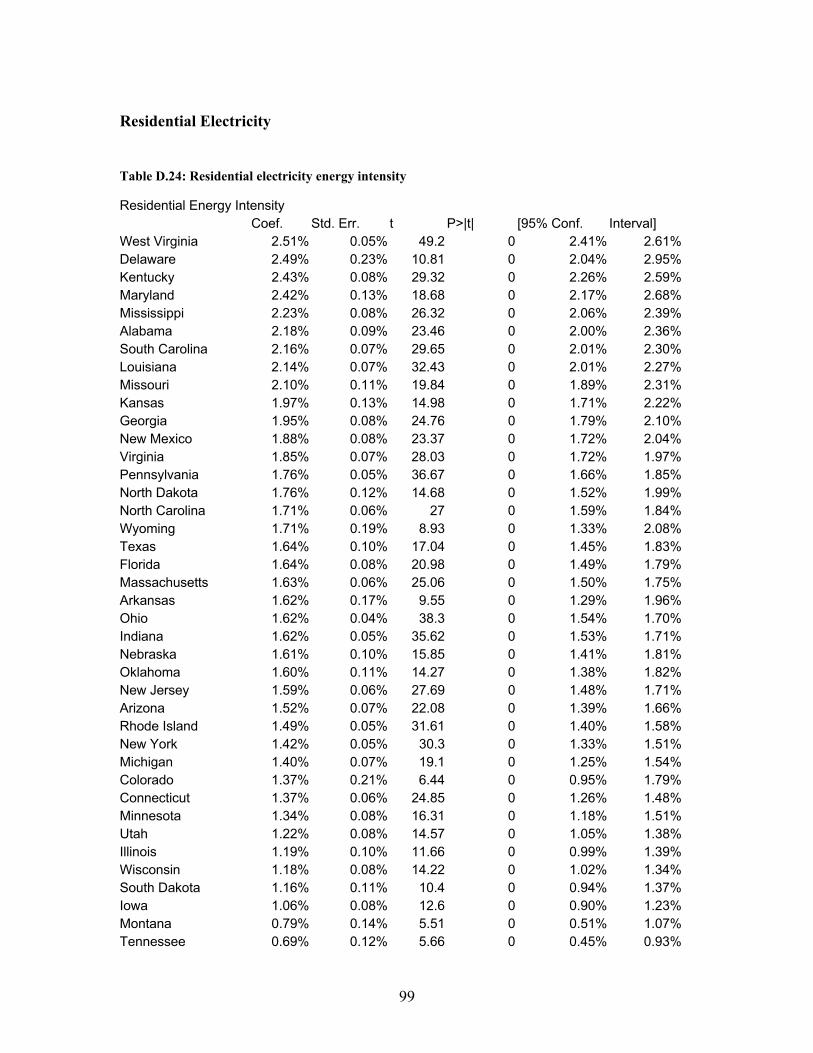
99

Residential Electricity

Table D.24: Residential electricity energy intensity

Residential Energy Intensity

Coef. Std. Err. t P>|t| [95% Conf. Interval]

West Virginia 2.51% 0.05% 49.2 0 2.41% 2.61%

Delaware 2.49% 0.23% 10.81 0 2.04% 2.95%

Kentucky 2.43% 0.08% 29.32 0 2.26% 2.59%

Maryland 2.42% 0.13% 18.68 0 2.17% 2.68%

Mississippi 2.23% 0.08% 26.32 0 2.06% 2.39%

Alabama 2.18% 0.09% 23.46 0 2.00% 2.36%

South Carolina 2.16% 0.07% 29.65 0 2.01% 2.30%

Louisiana 2.14% 0.07% 32.43 0 2.01% 2.27%

Missouri 2.10% 0.11% 19.84 0 1.89% 2.31%

Kansas 1.97% 0.13% 14.98 0 1.71% 2.22%

Georgia 1.95% 0.08% 24.76 0 1.79% 2.10%

New Mexico 1.88% 0.08% 23.37 0 1.72% 2.04%

Virginia 1.85% 0.07% 28.03 0 1.72% 1.97%

Pennsylvania 1.76% 0.05% 36.67 0 1.66% 1.85%

North Dakota 1.76% 0.12% 14.68 0 1.52% 1.99%

North Carolina 1.71% 0.06% 27 0 1.59% 1.84%

Wyoming 1.71% 0.19% 8.93 0 1.33% 2.08%

Texas 1.64% 0.10% 17.04 0 1.45% 1.83%

Florida 1.64% 0.08% 20.98 0 1.49% 1.79%

Massachusetts 1.63% 0.06% 25.06 0 1.50% 1.75%

Arkansas 1.62% 0.17% 9.55 0 1.29% 1.96%

Ohio 1.62% 0.04% 38.3 0 1.54% 1.70%

Indiana 1.62% 0.05% 35.62 0 1.53% 1.71%

Nebraska 1.61% 0.10% 15.85 0 1.41% 1.81%

Oklahoma 1.60% 0.11% 14.27 0 1.38% 1.82%

New Jersey 1.59% 0.06% 27.69 0 1.48% 1.71%

Arizona 1.52% 0.07% 22.08 0 1.39% 1.66%

Rhode Island 1.49% 0.05% 31.61 0 1.40% 1.58%

New York 1.42% 0.05% 30.3 0 1.33% 1.51%

Michigan 1.40% 0.07% 19.1 0 1.25% 1.54%

Colorado 1.37% 0.21% 6.44 0 0.95% 1.79%

Connecticut 1.37% 0.06% 24.85 0 1.26% 1.48%

Minnesota 1.34% 0.08% 16.31 0 1.18% 1.51%

Utah 1.22% 0.08% 14.57 0 1.05% 1.38%

Illinois 1.19% 0.10% 11.66 0 0.99% 1.39%

Wisconsin 1.18% 0.08% 14.22 0 1.02% 1.34%

South Dakota 1.16% 0.11% 10.4 0 0.94% 1.37%

Iowa 1.06% 0.08% 12.6 0 0.90% 1.23%

Montana 0.79% 0.14% 5.51 0 0.51% 1.07%

Tennessee 0.69% 0.12% 5.66 0 0.45% 0.93%

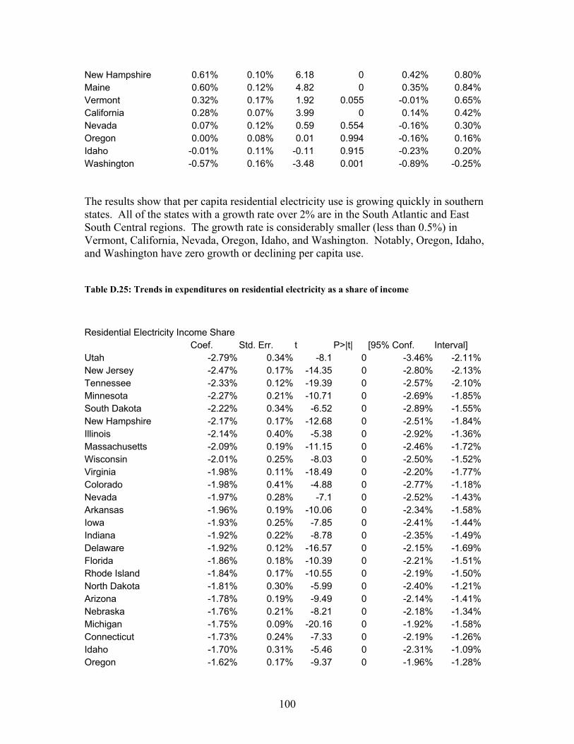
100

New Hampshire 0.61% 0.10% 6.18 0 0.42% 0.80%

Maine 0.60% 0.12% 4.82 0 0.35% 0.84%

Vermont 0.32% 0.17% 1.92 0.055 -0.01% 0.65%

California 0.28% 0.07% 3.99 0 0.14% 0.42%

Nevada 0.07% 0.12% 0.59 0.554 -0.16% 0.30%

Oregon 0.00% 0.08% 0.01 0.994 -0.16% 0.16%

Idaho -0.01% 0.11% -0.11 0.915 -0.23% 0.20%

Washington -0.57% 0.16% -3.48 0.001 -0.89% -0.25%

The results show that per capita residential electricity use is growing quickly in southern

states. All of the states with a growth rate over 2% are in the South Atlantic and East

South Central regions. The growth rate is considerably smaller (less than 0.5%) in

Vermont, California, Nevada, Oregon, Idaho, and Washington. Notably, Oregon, Idaho,

and Washington have zero growth or declining per capita use.

Table D.25: Trends in expenditures on residential electricity as a share of income

Residential Electricity Income Share

Coef. Std. Err. t P>|t| [95% Conf. Interval]

Utah -2.79% 0.34% -8.1 0 -3.46% -2.11%

New Jersey -2.47% 0.17% -14.35 0 -2.80% -2.13%

Tennessee -2.33% 0.12% -19.39 0 -2.57% -2.10%

Minnesota -2.27% 0.21% -10.71 0 -2.69% -1.85%

South Dakota -2.22% 0.34% -6.52 0 -2.89% -1.55%

New Hampshire -2.17% 0.17% -12.68 0 -2.51% -1.84%

Illinois -2.14% 0.40% -5.38 0 -2.92% -1.36%

Massachusetts -2.09% 0.19% -11.15 0 -2.46% -1.72%

Wisconsin -2.01% 0.25% -8.03 0 -2.50% -1.52%

Virginia -1.98% 0.11% -18.49 0 -2.20% -1.77%

Colorado -1.98% 0.41% -4.88 0 -2.77% -1.18%

Nevada -1.97% 0.28% -7.1 0 -2.52% -1.43%

Arkansas -1.96% 0.19% -10.06 0 -2.34% -1.58%

Iowa -1.93% 0.25% -7.85 0 -2.41% -1.44%

Indiana -1.92% 0.22% -8.78 0 -2.35% -1.49%

Delaware -1.92% 0.12% -16.57 0 -2.15% -1.69%

Florida -1.86% 0.18% -10.39 0 -2.21% -1.51%

Rhode Island -1.84% 0.17% -10.55 0 -2.19% -1.50%

North Dakota -1.81% 0.30% -5.99 0 -2.40% -1.21%

Arizona -1.78% 0.19% -9.49 0 -2.14% -1.41%

Nebraska -1.76% 0.21% -8.21 0 -2.18% -1.34%

Michigan -1.75% 0.09% -20.16 0 -1.92% -1.58%

Connecticut -1.73% 0.24% -7.33 0 -2.19% -1.26%

Idaho -1.70% 0.31% -5.46 0 -2.31% -1.09%

Oregon -1.62% 0.17% -9.37 0 -1.96% -1.28%

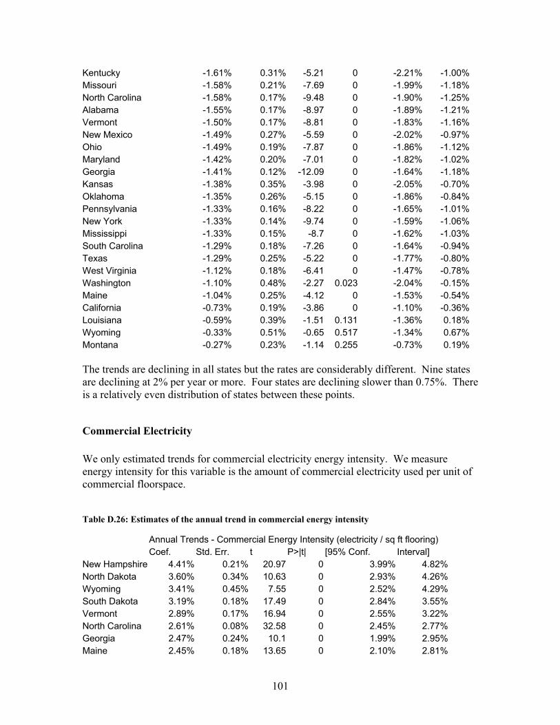
101

Kentucky -1.61% 0.31% -5.21 0 -2.21% -1.00%

Missouri -1.58% 0.21% -7.69 0 -1.99% -1.18%

North Carolina -1.58% 0.17% -9.48 0 -1.90% -1.25%

Alabama -1.55% 0.17% -8.97 0 -1.89% -1.21%

Vermont -1.50% 0.17% -8.81 0 -1.83% -1.16%

New Mexico -1.49% 0.27% -5.59 0 -2.02% -0.97%

Ohio -1.49% 0.19% -7.87 0 -1.86% -1.12%

Maryland -1.42% 0.20% -7.01 0 -1.82% -1.02%

Georgia -1.41% 0.12% -12.09 0 -1.64% -1.18%

Kansas -1.38% 0.35% -3.98 0 -2.05% -0.70%

Oklahoma -1.35% 0.26% -5.15 0 -1.86% -0.84%

Pennsylvania -1.33% 0.16% -8.22 0 -1.65% -1.01%

New York -1.33% 0.14% -9.74 0 -1.59% -1.06%

Mississippi -1.33% 0.15% -8.7 0 -1.62% -1.03%

South Carolina -1.29% 0.18% -7.26 0 -1.64% -0.94%

Texas -1.29% 0.25% -5.22 0 -1.77% -0.80%

West Virginia -1.12% 0.18% -6.41 0 -1.47% -0.78%

Washington -1.10% 0.48% -2.27 0.023 -2.04% -0.15%

Maine -1.04% 0.25% -4.12 0 -1.53% -0.54%

California -0.73% 0.19% -3.86 0 -1.10% -0.36%

Louisiana -0.59% 0.39% -1.51 0.131 -1.36% 0.18%

Wyoming -0.33% 0.51% -0.65 0.517 -1.34% 0.67%

Montana -0.27% 0.23% -1.14 0.255 -0.73% 0.19%

The trends are declining in all states but the rates are considerably different. Nine states

are declining at 2% per year or more. Four states are declining slower than 0.75%. There

is a relatively even distribution of states between these points.

Commercial Electricity

We only estimated trends for commercial electricity energy intensity. We measure

energy intensity for this variable is the amount of commercial electricity used per unit of

commercial floorspace.

Table D.26: Estimates of the annual trend in commercial energy intensity

Annual Trends - Commercial Energy Intensity (electricity / sq ft flooring)

Coef. Std. Err. t P>|t| [95% Conf. Interval]

New Hampshire 4.41% 0.21% 20.97 0 3.99% 4.82%

North Dakota 3.60% 0.34% 10.63 0 2.93% 4.26%

Wyoming 3.41% 0.45% 7.55 0 2.52% 4.29%

South Dakota 3.19% 0.18% 17.49 0 2.84% 3.55%

Vermont 2.89% 0.17% 16.94 0 2.55% 3.22%

North Carolina 2.61% 0.08% 32.58 0 2.45% 2.77%

Georgia 2.47% 0.24% 10.1 0 1.99% 2.95%

Maine 2.45% 0.18% 13.65 0 2.10% 2.81%

102

Alabama 2.40% 0.29% 8.43 0 1.85% 2.96%

Delaware 2.35% 0.21% 11.27 0 1.94% 2.76%

Maryland 2.34% 0.69% 3.41 0.001 0.99% 3.68%

Mississippi 2.32% 0.27% 8.75 0 1.80% 2.84%

Michigan 2.24% 0.25% 9.03 0 1.76% 2.73%

Missouri 2.11% 0.11% 18.8 0 1.89% 2.33%

West Virginia 2.06% 0.11% 19.46 0 1.85% 2.27%

New Mexico 2.04% 0.18% 11.63 0 1.69% 2.38%

Nebraska 2.01% 0.17% 12.11 0 1.68% 2.34%

Utah 1.99% 0.18% 11.21 0 1.64% 2.33%

New Jersey 1.95% 0.11% 18.44 0 1.74% 2.16%

Pennsylvania 1.81% 0.07% 25.32 0 1.67% 1.95%

Minnesota 1.70% 0.10% 17.38 0 1.51% 1.89%

Indiana 1.63% 0.12% 13.33 0 1.39% 1.87%

Rhode Island 1.62% 0.11% 14.08 0 1.39% 1.84%

Ohio 1.59% 0.14% 11.42 0 1.31% 1.86%

New York 1.58% 0.07% 21.73 0 1.44% 1.72%

Colorado 1.57% 0.26% 6.02 0 1.06% 2.08%

Montana 1.55% 0.54% 2.86 0.004 0.49% 2.61%

Florida 1.53% 0.09% 16.53 0 1.35% 1.72%

Kansas 1.41% 0.07% 19.97 0 1.28% 1.55%

Arkansas 1.38% 0.15% 9.41 0 1.09% 1.66%

Wisconsin 1.35% 0.10% 13.99 0 1.16% 1.54%

Kentucky 1.31% 0.07% 17.86 0 1.17% 1.45%

Texas 1.30% 0.09% 15.27 0 1.13% 1.47%

Connecticut 1.29% 0.09% 15 0 1.12% 1.46%

Massachusetts 1.26% 0.08% 15.03 0 1.10% 1.43%

Virginia 1.22% 0.07% 17.12 0 1.08% 1.36%

Iowa 1.21% 0.14% 8.48 0 0.93% 1.48%

South Carolina 1.18% 0.14% 8.62 0 0.91% 1.45%

Washington 0.86% 0.28% 3.06 0.002 0.31% 1.42%

Oklahoma 0.69% 0.17% 3.97 0 0.35% 1.03%

Arizona 0.64% 0.18% 3.58 0 0.29% 0.99%

Illinois 0.63% 0.14% 4.59 0 0.36% 0.90%

Oregon 0.56% 0.22% 2.59 0.01 0.14% 0.99%

Idaho 0.47% 0.18% 2.61 0.009 0.12% 0.83%

Louisiana 0.47% 0.08% 5.54 0 0.30% 0.64%

Nevada 0.20% 0.61% 0.34 0.737 -0.98% 1.39%

California -0.66% 0.10% -6.63 0 -0.86% -0.47%

Tennessee -2.27% 1.71% -1.33 0.185 -5.64% 1.09%

The trend is increasing in almost all states and New Hampshire, North Dakota, Wyoming,

and South Dakota have rapid growth over 3%. Ten states are growing at less than 1%.

California and Tennessee have negative trends.

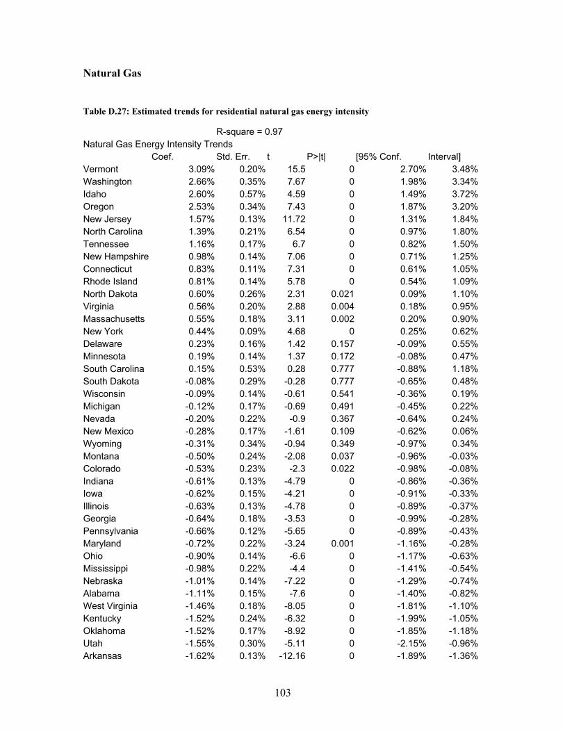
103

Natural Gas

Table D.27: Estimated trends for residential natural gas energy intensity

R-square = 0.97

Natural Gas Energy Intensity Trends

Coef. Std. Err. t P>|t| [95% Conf. Interval]

Vermont 3.09% 0.20% 15.5 0 2.70% 3.48%

Washington 2.66% 0.35% 7.67 0 1.98% 3.34%

Idaho 2.60% 0.57% 4.59 0 1.49% 3.72%

Oregon 2.53% 0.34% 7.43 0 1.87% 3.20%

New Jersey 1.57% 0.13% 11.72 0 1.31% 1.84%

North Carolina 1.39% 0.21% 6.54 0 0.97% 1.80%

Tennessee 1.16% 0.17% 6.7 0 0.82% 1.50%

New Hampshire 0.98% 0.14% 7.06 0 0.71% 1.25%

Connecticut 0.83% 0.11% 7.31 0 0.61% 1.05%

Rhode Island 0.81% 0.14% 5.78 0 0.54% 1.09%

North Dakota 0.60% 0.26% 2.31 0.021 0.09% 1.10%

Virginia 0.56% 0.20% 2.88 0.004 0.18% 0.95%

Massachusetts 0.55% 0.18% 3.11 0.002 0.20% 0.90%

New York 0.44% 0.09% 4.68 0 0.25% 0.62%

Delaware 0.23% 0.16% 1.42 0.157 -0.09% 0.55%

Minnesota 0.19% 0.14% 1.37 0.172 -0.08% 0.47%

South Carolina 0.15% 0.53% 0.28 0.777 -0.88% 1.18%

South Dakota -0.08% 0.29% -0.28 0.777 -0.65% 0.48%

Wisconsin -0.09% 0.14% -0.61 0.541 -0.36% 0.19%

Michigan -0.12% 0.17% -0.69 0.491 -0.45% 0.22%

Nevada -0.20% 0.22% -0.9 0.367 -0.64% 0.24%

New Mexico -0.28% 0.17% -1.61 0.109 -0.62% 0.06%

Wyoming -0.31% 0.34% -0.94 0.349 -0.97% 0.34%

Montana -0.50% 0.24% -2.08 0.037 -0.96% -0.03%

Colorado -0.53% 0.23% -2.3 0.022 -0.98% -0.08%

Indiana -0.61% 0.13% -4.79 0 -0.86% -0.36%

Iowa -0.62% 0.15% -4.21 0 -0.91% -0.33%

Illinois -0.63% 0.13% -4.78 0 -0.89% -0.37%

Georgia -0.64% 0.18% -3.53 0 -0.99% -0.28%

Pennsylvania -0.66% 0.12% -5.65 0 -0.89% -0.43%

Maryland -0.72% 0.22% -3.24 0.001 -1.16% -0.28%

Ohio -0.90% 0.14% -6.6 0 -1.17% -0.63%

Mississippi -0.98% 0.22% -4.4 0 -1.41% -0.54%

Nebraska -1.01% 0.14% -7.22 0 -1.29% -0.74%

Alabama -1.11% 0.15% -7.6 0 -1.40% -0.82%

West Virginia -1.46% 0.18% -8.05 0 -1.81% -1.10%

Kentucky -1.52% 0.24% -6.32 0 -1.99% -1.05%

Oklahoma -1.52% 0.17% -8.92 0 -1.85% -1.18%

Utah -1.55% 0.30% -5.11 0 -2.15% -0.96%

Arkansas -1.62% 0.13% -12.16 0 -1.89% -1.36%

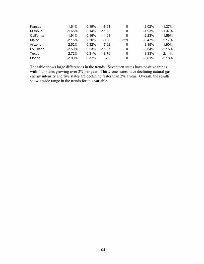
104

Kansas -1.64% 0.19% -8.61 0 -2.02% -1.27%

Missouri -1.65% 0.14% -11.63 0 -1.93% -1.37%

California -1.91% 0.16% -11.68 0 -2.23% -1.59%

Maine -2.15% 2.20% -0.98 0.329 -6.47% 2.17%

Arizona -2.52% 0.32% -7.92 0 -3.15% -1.90%

Louisiana -2.59% 0.23% -11.37 0 -3.04% -2.15%

Texas -2.72% 0.31% -8.76 0 -3.33% -2.11%

Florida -2.90% 0.37% -7.9 0 -3.61% -2.18%

The table shows large differences in the trends. Seventeen states have positive trends

with four states growing over 2% per year. Thirty-one states have declining natural gas

energy intensity and five states are declining faster than 2% a year. Overall, the results

show a wide range in the trends for this variable.