INFORMATION TRANSMISSION UNDER THE SHADOW OF THE FUTURE:

AN EXPERIMENT

EMANUEL VESPA AND ALISTAIR J. WILSON

ABSTRACT. We experimentally examine how information transmission functions in an ongoing

relationship. Where the one-shot literature documents substantial over-communication and pref-

erences for honesty, in our repeated setting the outcomes are more consistent with uninformative

babbling outcomes. This is particularly surprising as honest revelation is supportable as an equilib-

rium outcome in our repeated setting. We show that the inefficient outcomes we find are driven by a

coordination failure. More specifically, we show that in order to sustain honest revelation, the focal

dynamic punishments in this environment require a coordination on the payment of “information

rents.”

“’tis like the breath of an unfee’d lawyer. You gave me nothing for’t. Can you make no

use of nothing[?]”

– King Lear, (1.4.642–44, 1.4.660–62)

Our paper examines the intersection of two key areas of current economic research: the degree

to which information is shared by interested parties and how repeated interaction in long-run re-

lationships can open up the possibility for more-efficient outcomes. Our main question focuses

on whether repeated interaction can produce efficiency-improvements to the transmission of infor-

mation. Our findings for repeated interaction indicate a qualified positive, where the main motive

behind greater information transmission when we observe it are strategic: information is shared

only when there is compensation. However, repeated interaction on its own is not sufficient to

generate an efficiency gain; overcoming coordination hurdles on how to share efficiency gains are

critical to successful outcomes.

From a theoretical perspective, repeated interactions clearly offer the potential for gains with in-

formation transmission. While full revelation is not an equilibrium in one-shot settings such as

Date: October, 2016.We would like to thank: Ted Bergstrom, Andreas Blume, Gabriele Camera, Katie and Lucas Coffman, John Duffy,Rod Garratt, PJ Healy, Andrew Kloosterman, John Kagel, Tom Palfrey, Joel Sobel, Lise Vesterlund, Sevgi Yuksel,as well as seminar audiences at Ohio State, Penn State, Arizona, Pittsburgh, UC Berkeley, UC Irvine (SWEBE), UCRiverside, UC Santa Cruz, UC San Diego, UC Santa Barbara, UCL, Virginia, SITE and the international meeting ofthe ESA in Jerusalem. The authors gratefully acknowledge financial support from the NSF (SES-1629193). Vespa:vespa@ucsb.edu; Wilson: alistair@pitt.edu.

1

Crawford and Sobel (1982), it can be supported if parties interact repeatedly. Moreover, two cur-

rent literatures taken independently provide an optimistic prior. First, the experimental literature

on one-shot cheap-talk games already documents over-transmission of information relative to theo-

retical predictions. Second, a literature examining repeated interaction in prisoners’ dilemmas (see

Dal Bó and Fréchette, 2016, for a survey) shows that repeated interactions can improve efficiency

through the use of dynamic strategies. However, caution may be warranted when extending these

two results to repeated cheap talk. With respect to the first finding, a sender may be discouraged

from being systematically honest if her partner is using the extra information solely to her own ad-

vantage. In addition, the coordination problem in this environment is not a trivial extension of that

in a repeated prisoners’ dilemma. In a repeated cheap talk environment many efficient equilibria

can be supported depending on how sender and receivers share efficiency gains. In fact a subtle

trade-off emerges: for the receiver to get a higher share in equilibrium, the off-path punishments

they use must be more severe.

We set up a simple sender-receiver environment with uncertainty over a payoff-relevant state. In

our stage game, an investment opportunity is either good or bad with equal chance. An informed

expert (the sender, she) observes the investment quality and provides a recommendation to the

decision-maker (DM, the receiver, he), who chooses a level of investment. We restrict the sender

to choose one of two possible recommendations—invest or don’t invest—where her payoffs are

increasing in the decision-maker’s investment level regardless of the underlying quality. The DM’s

ex post payoff is maximized by full investment in the good state, and no investment in the bad

state. But, in addition to full and no investment, the DM can also select an intermediate partial

investment level, which is the best response to his initial prior on the opportunity.

The incentives create a clear strategic tension. While there is mutual benefit from full investment

for a good opportunity, the preferences of the two parties are completely misaligned for a bad one.

In one-shot interactions the wedge between honest revelation and self-interest for low-quality in-

vestments leads to substantial inefficiencies in equilibrium. For our particular setting the unique

equilibrium prediction is that the DM chooses his uninformed best response (here partial invest-

ment) at all quality levels. This uninformative “babbling” outcome is ex post inefficient, as full

investment for good opportunities makes both expert and DM better off.

In expectation this environment has distinctly similar to a prisoner’s dilemma (PD) game: a Pareto

efficient outcome that cannot be achieved in one-shot interactions as each party benefits from a

deviation. (The sender dishonestly claiming a good state, the DM reducing their investment for

revealed bad states.) Given the parallels to a prisoner’s dilemma, our main paper asks an obvious

question: to what extent can repetition increase efficiency? Theoretically, so long as each party

values the future enough then more-efficient equilibria can be constructed. Much like an indef-

initely repeated PD, history-dependent strategies can implement efficient play (and many other2

other outcomes) in equilibrium. However, unlike the PD, a novel coordination tradeoff emerges

between: (i) harshness of the punishments; and (ii) how the surplus generated from revelation is

distributed.

From the point of view of the DM, the first-best outcome is full-revelation of the investment qual-

ity by the expert, and full-extraction of the surplus—full investment for good opportunities, no

investment for bad. The path of play for full extraction is cognitively simple for the DM, choosing

his most-preferred outcome given the revealed quality. Though coordination on this path is also

simple for the expert, as none of the gains are shared the net incentive to truthfully reveal bad op-

portunities must be driven by punishment. While possible in equilibrium, if DMs hope to support

full extraction, they must use complex punishments that are (at least temporarily) painful to both

parties. Moreover, such punishments must eventually recoordinate on efficient play.

In contrast to full extraction, simpler punishments can be used to support information revelation

if the DM shares the efficiency gains from revelation with the expert—what we will refer to as an

“information rent.” In particular, given a large-enough information rent, an intuitively appealing

dynamic punishment can be used to support efficient play in equilibrium: reversion to the uninfor-

mative babbling outcome. In the theoretical section of the paper, we show that the choice between

coordinating on harsher punishments than the static Nash outcome, or coordination on the payment

of information rents, is not unique to our experimental setting. Instead, under typical concavity as-

sumptions on preferences, information rents are a necessary component of efficient play supported

by Nash-triggers, even for future discount rates arbitrarily close to one.

While the literature on repeated play has found evidence for coordination on more-lenient punish-

ments than Nash reversion (for instance, see Fudenberg et al., 2010), there is little evidence for

coordination on harsher punishments. This behavioral observation motivates a refinement for folk

theorems: a proscription on punishments harsher than the worst Nash equilibrium. In our sender-

receiver environment, this simple refinement has clear implications: First, if punishments can be

no harsher than Nash, whenever efficient play does emerge it must necessarily involve the pay-

ment of an information rent. Second, as a parallel to the first implication, solving the coordination

problem to achieve efficient play in our environment is much tougher than standard repeated PD

games.

Our paper’s experimental design first focuses on measuring the effects of repeated play in our

cheap-talk environment. A Partners treatment, where matchings are fixed within all periods of

a supergame, is compared to a Strangers control in which participants are matched with a new

subject every period. If repeated interaction selects equilibria with greater information transfer,

we should observe large efficiency differences between the two treatments. Instead, we find that

the modal responses in both treatments reflects the uninformative babbling outcome. While we3

do document differences in the expected direction—more information is transmitted in our Part-

ners treatment—the effects are economically small. While this result is certainly surprising when

set against the one-shot cheap-talk and infinite-horizon PD literatures, it is less so when viewed

through the lens of the coordination problems we outline for this environment.

To investigate whether the babbling-like results in our repeated environment are driven by coordi-

nation failure, we conduct an additional treatment which alleviates this problem. Though identical

to our Partners treatment for the initial supergames, in the second part of our Chat treatments we

let participants freely communicate before the supergame begins. While behavior is not distin-

guishable from Partners before the coordination device is provided, large differences emerge from

the very first supergame where they have access to it. Where the comparable late-stage Partners’

supergames are 24 percent efficient, efficiency is 86 percent in the Chat treatment. Moreover, a

detailed examination of the chat exchanges clearly indicates that the large-majority of subjects are

exactly coordinated on an efficient information rents outcome.1 That this outcome emerges at the

very first opportunity to explicitly coordinate points to subjects’ clear understandings of how to

(jointly) solve their coordination problem.

The Chat treatment results indicate that where the coordination problem is relaxed, subjects pick

out paths of play where information rents are provided to the expert. Our last two treatments inves-

tigate if it is possible to achieve efficient outcomes without pre-play communication by relaxing

coordination difficulties. Notice that coordination can be thought of as having two components.

Depending on whether information is revealed or not, coordination can be on an efficient or on an

inefficient outcome. But when information is fully revealed, subjects need to solve distributional

issues and coordinate on one of the possible efficient equilibria. The first manipulation provides a

coordination device aimed at making efficient revealing outcomes easier to support. Here our re-

sults show no effect relative to Partners, with modal behavior best characterized as uninformative.

Our second manipulation instead provides a coordination device that helps address the distribu-

tional concerns key to the information rent. In this second manipulation we observe a significant

increase in efficiency relative to Partners, attaining approximately 60 percent of the efficiency

gains in the Chat treatment. Solving the coordination problem over the distribution is critical for

successful outcomes in this environment.

The evidence from our experimental treatments points to the importance of information rents,

an idea that goes back to an older literature on regulating a monopolist’s price (see Baron and

Besanko, 1984; Laffont and Tirole, 1988). To retain incentives for honest revelation on profitabil-

ity, that literature shows that a monopolist must be given some positive profits along the path,

as otherwise they have no incentive to provide information against their own interests. While our

infinite-horizon setting admits the equilibrium possibility for full revelation without a rent (through

1In contrast, full extraction by the DM, which requires harsh supporting punishments is hardly ever coordinated upon.4

harsh punishments) the data indicates that such outcomes are not selected. Once a relationship is

deceptive, babbling is the absorbing outcome across our treatments. Where dynamic strategies of

the game are restricted to such punishments, information rents become necessary for efficient play.

Per the quote that we open the paper with, honest advice must be paid for. But the context of

that quote is important here too, and speaks to the difficulty of coordination. When we are being

advised, we can focus too myopically on the specific advice given, and forget that our choices have

implications for those providing their expertise. Where we fail to reward those providing honest

information today, one outcome is to degrade the extent to which we get honest advice tomorrow.

We next present a brief review of the literature. In Section 2 we outline our main treatment and

control, along with the theoretical predictions. Section 3 contains the results from these two treat-

ments. In Section 4 we introduce our Chat treatment and the results. Section 5 follows with a

discussion of two weaker coordination-device treatments. Finally, in Section 6 we discuss our

results and conclude.

1.1. Literature. Per the introductory paragraph, the paper is most clearly related to two litera-

tures: information transmission and repeated games. For the first, the theory is related to cheap

talk games examining an informed but biased sender, where the most-prominent paper in this lit-

erature is Crawford and Sobel (1982). The fundamental finding here is that full revelation is ruled

out (for the one-shot game), with at best partial revelation in equilibrium. The model has been

examined in experimental studies, where the main results are that more information is exchanged

than predicted by the theory.2

Outside of the Crawford and Sobel framework Gneezy (2005) compares the willingness of an

informed sender to signal the payoff-maximizing action to a receiver.3 Despite large monetary

losses from honest revelation, the paper documents substantial information transfer. Comparing the

sender behavior to decisions in a matched dictator game, the paper concludes there is a preference

for honesty.4 Further evidence for lying-aversion is given in Fischbacher and Föllmi-Heusi (2013),

introducing a die-rolling task where the subjects are paid based on their own private roll of a

die. While the die outcomes are private, lying can be detected in aggregate by comparing the

distributions of reports to the known generating process. Such deception environments are most

comparable to the bad state in our game—with a direct tension between truthful reporting and

self-interest. However, the predicted effects of lying aversion are toward increased efficiency, in

opposition to our results.

2See Dickhaut et al. (1995); Cai and Wang (2006); Wang et al. (2010). Also see Blume et al. (1998) for an examinationsof the evolutions of message meaning.3Receivers here are ignorant of the game form, only knowing that they have two available actions.4Some of the excess revelation in Gneezy can be explained as failed strategizing by senders believing the receiver willreverse their advice (see Sutter, 2009), though only 20 percent of receivers do so. See also Hurkens and Kartik (2009),which demonstrates that lying aversion may not vary with the harm done to others.

5

Our paper is also related to the literature on conditional cooperation in repeated games. Much of the

theoretical literature here focuses on documenting the generality and breadth of the indeterminacy

of prediction via folk theorems.5 While recent theoretical work examines dynamic sender-receiver

environments with persistent state variables (see Renault et al., 2013; Golosov et al., 2014), our

game has a much simpler separable structure.6 With perfect-monitoring, standard repeated-game

constructions can be used to show the existence of more-efficient outcomes. Though we do not

make a technical contribution to this literature, we do outline a practically motivated refinement

for these games that reduces the theoretical indeterminacy: punishments should be simple.

A robust experimental literature on behavior in repeated PD-games has examined predictable fea-

tures of selection. Surveying the literature and conducting a meta-analysis Dal Bó and Fréchette

(2016) show that cooperation being supportable as an equilibrium outcome is necessary.7 But

more than this, they show that the difficulty of the coordination problem (here measuring the ef-

ficiency gains available from cooperation measured relative to the temptations and risks from a

deviations) are predictive of selection. Further, the evidence from the meta-study suggests that

selected punishments are frequently less harsh than grim-triggers, with Tit-for-Tat is a frequently

detected strategy. In addition, the finding is that punishment phases in imperfect public monitoring

games are typically forgiving (see in particular Fudenberg et al., 2010). In dynamic game settings

with state-variables Vespa and Wilson (2015) indicates that more-cooperative outcomes than the

history-independent Markov perfect equilibria (MPE) can be sustained, but that the most-frequent

punishments are reversions to the MPE. While some papers have examined the selection of more

costly punishments than Nash reversion, none find that this selection is useful in supporting higher

payoffs.8 To our knowledge, our paper is the first to examine the tradeoffs between sharing the

gains from the selection of more-efficient equilibria and the selection of punishments.9

5See Fudenberg and Maskin (1986); Fudenberg et al. (1994); Dutta (1995)6For an experiment here see Ettinger and Jehiel (2015), which examines a repeated sender-receiver game, where thesender has a persistent type, mirroring the Sobel (1985) model of credibility.7For the effect of pre-play communication in repeated PD-games see Arechar et al. (2016) and references therein. Alsosee the literature on team communication, in particular Cooper and Kagel (2005) and Kagel and McGee (2016).8Dreber et al. (2008) find that where costly punishments are used they are unsuccessful at supporting better outcomes;similarly, Wilson and Wu (2016) find subjects employing a dominated strategy (termination) as a costly punishment,but without a forward effect in the supergame.9Outside of the infinite-horizon setting, Brown et al. (2004) show that gains over the inefficient equilibrium predictionneed to be shared for efficient outcomes to emerge in their relational contracting setting. In an infinite-horizon setting,these results can be rationalized as the effective punishments here are based on termination and rematching. If gains arenot shared in one relationship, but are in the larger population, the simple punishment is to terminate the relationship,and sharing gains is necessary.

6

2. DESIGN: THEORY AND HYPOTHESES

In this section we present the basic environment that we study in the laboratory, a streamlined

version of a repeated cheap-talk game. A straightforward alternative would be to directly use

Crawford and Sobel (1982) as our stage-game. Instead, we simplify the standard stage-game for

two reasons. First, with a simpler stage game that keeps the main tensions we can reduce the

complexity naturally added by repetition. Second, the analysis and interpretation of the data will

be more direct.

The stage game of the infinite-horizon sender-receiver environment that we study is depicted in

Figure 1. The game unfolds as follows: i) Nature chooses a state of the world θ ∈ {G(ood), B(ad)},

with equal probability;10 ii) the Sender player perfectly observes the state θ and chooses a message

m ∈ {Invest,Don’t Invest}; iii) the Receiver player observes the message m but not the state, and

chooses an action a ∈ {Full, Partial,None} ; iv) at the end of each stage game the entire history of

the period (θ,m, a) becomes common knowledge.11

Payoffs for the game are as follows: The sender’s payoff is given by

u(a) =

1 if a = Full,

u0 if a = Partial,

0 if a = None,

while the receiver’s payoff is

v(a, θ) =

1 if (a, θ) ∈ {(Full, Good),(None,Bad)} ,

v0 if a = Partial,

0 otherwise.

The parameters u0 ∈ (0, 1) and v0 >12

represent how the two participants rank partial investment.

Conditional on the Good state, the two players share common interests: the investment actions are

Pareto ranked, from best to worst, by Full to Partial to None. However, conditional on the Bad

state the Sender and Receiver have diametrically opposed preferences over the selected actions. In

particular, when θ =Bad, the Full investment choice distributes the entire amount to the sender,

while None distributes everything to the receiver. Finally, the preference assumption v0 > 1/2 for

10Selecting either state with equal probability is akin to having a uniform distribution over a continuous state-space.An advantage of this choice is that the distribution of nature’s moves provides no ex-ante information for receivers. Ifone state was selected with a higher probability, then the receiver’s choice can be affected by both the distribution ofnature and the message, making it more difficult to identify the effect of the sender’s behavior on the receiver.11In the laboratory we use a neutral frame where the state, messages and recommendations are labeled as either ‘left’(for good/invest/full investment) or ‘right’ (for bad/don’t/no investment) with ‘middle’ the label for the safe partial-investment action. Instructions are available in the Online Appendix to the paper.

7

Bad (12)Good (1

2) Nature

Don’t

Invest

Sender

Don’t

Invest

Sender

Receiver

Receiver

None

0, 0

Full

1, 1

Part.

u0, v0

None

0, 1

Full

1, 0

Part.

u0, v0

None

0, 0

Full

1, 1

Part.

u0, v0

None

0, 1

Full

1, 0

Part.

u0, v0

FIGURE 1. Stage Game

the receiver is chosen so that ex ante the Partial investment action is preferred to either full or no

investment.12

The informed sender’s chosen signal m affects neither players’ payoff directly, and so this is a

cheap-talk environment. Moreover the sender’s payoff here is state independent, affected by the

chosen action only. In terms of theoretical predictions for the stage game, this means that all perfect

Bayesian equilibrium (PBE) involve the receiver choosing a = Partial with certainty.13

2.1. Experimental Design. Our experimental design will examine a repeated (infinite-horizon)

version of the stage game given in Figure 1, which we will refer to as a supergame. We choose

u0 = 1/3 and v0 = 2/3 so that the payoffs in the bad state are constant sum for all actions, and in

that way it is a purely distributional state.

12This is under the assumption of risk-neutrality over the payoffs. In order to move away from the babbling predictionthe receiver must be risk-loving to a very strong degree (a CRRA coefficient -0.71 or below). For risk-neutral prefer-ences a posterior belief on either state above v0 is required for partial investment not to be the best response, with thisrequirement increasing in their risk aversion (effectively pushing up the value of v0).13The outcome in which the receiver takes the uninformed best-response is referred to as babbling. One reason weintroduce a third action for the receiver is to make the uninformed best response here unique. For a stage game withonly two choices: (Full and None) the receiver can implement babbling by ignoring the message and selecting Full,None, or a mixture. In all cases the expected payoff is 1/2.

8

After each completed period in the supergame we induce a δ = 3/4 probability that the supergame

continues into another period, and a (1 − δ) probability that the supergame stops. From the point

of view of a risk-neutral subject in period one, the expected payoffs for the infinite sequence of

possible states/messages/actions for the sender and receiver, respectively, is proportional to:

U ({mt(θ), at(m)}∞t=1) = (1− δ)

∑∞t=1 δ

t−1Eθu (a

t (mt (θ))) ,

V ({mt(θ), at(m)}∞t=1) = (1− δ)

∑∞t=1 δ

t−1Eθv (a

t (mt (θ)) , θt) .

We will initially examine two treatments: In the first, which we will call our Partners treatment, the

sender-receiver pair is fixed across the supergame. A sender participant i, and a receiver participant

j are therefore paired together in all supergame periods. A sender in period T > 1 observes the

history hTi =

{

θT ,{

θt, mti, a

tj

}T−1

t=1

}

when it is their turn to move, while the receiver observes

hTj =

{

mTi , {θ

t, mt, at}T−1t=1

}

.

In our second treatment, which we call Strangers, the sender-receiver pairings in each period are

random. A particular sender i is anonymously matched with a random sequence of receivers,

J(t). Similarly each receiver j is matched to a random sequence of senders, I(t). The sender’s

observed history is therefore hTi =

{

θT ,{

θt, mti, a

tJ(t)

}T−1

t=1

}

where they have no knowledge of

the particular receivers they have interacted with. Similarly, the receiver’s observable history in

each period is hTj =

{

mTJ(T ),

{

θt, mtJ(t), a

ti

}T−1

t=1

}

, where the receiver again does not know which

senders they have previously interacted with.14

2.2. Strangers Game. Given the random, anonymous matching, we treat each supergame in our

Strangers treatment as a sequence of one-shot games. Though the instructions, supergame lengths,

and potential payoffs are the same as our Partners treatment, subjects are unable to tie the previous

history to the presently matched participant. The shadow of the future can not work if future

behavior is independent of history. In principle, were δ large enough, more-efficient equilibria

are possible in the Strangers treatment, through “contagion” constructions. We will not focus on

such constructions for two reasons: First, experimental examination of contagion equilibria show

that they lack predictive power when they do exist.15 Second, given our choice of δ = 3/4 and

the particular random-matching protocol we use, such outcomes are not equilibria of the induced

session-level supergame.

14Moreover we guarantee senders and receivers in Strangers that the rematching process is makessure that they are never rematched to the same subject in two contiguous supergame periods: soPr {I(t) = I(t+ 1)}=Pr {J(t) = J(t+ 1)} = 0 for all t.15Duffy and Ochs (2009) finds no support for contagion equilibrium predictions. Camera and Casari (2009) show thatcontagion can be observed if subjects are provided the history of their anonymous match’s choices and the group sizeis small (the strongest evidence is for groups of four). Neither of these conditions is met in our design, where subjectsdo not observe their match’s previous choices, and the group size in our sessions consists of at least 14 participants.

9

� �

�

��

�

�

�

�����

��������

Babbling

Full Extraction

AlwaysFull

Inf. Rent

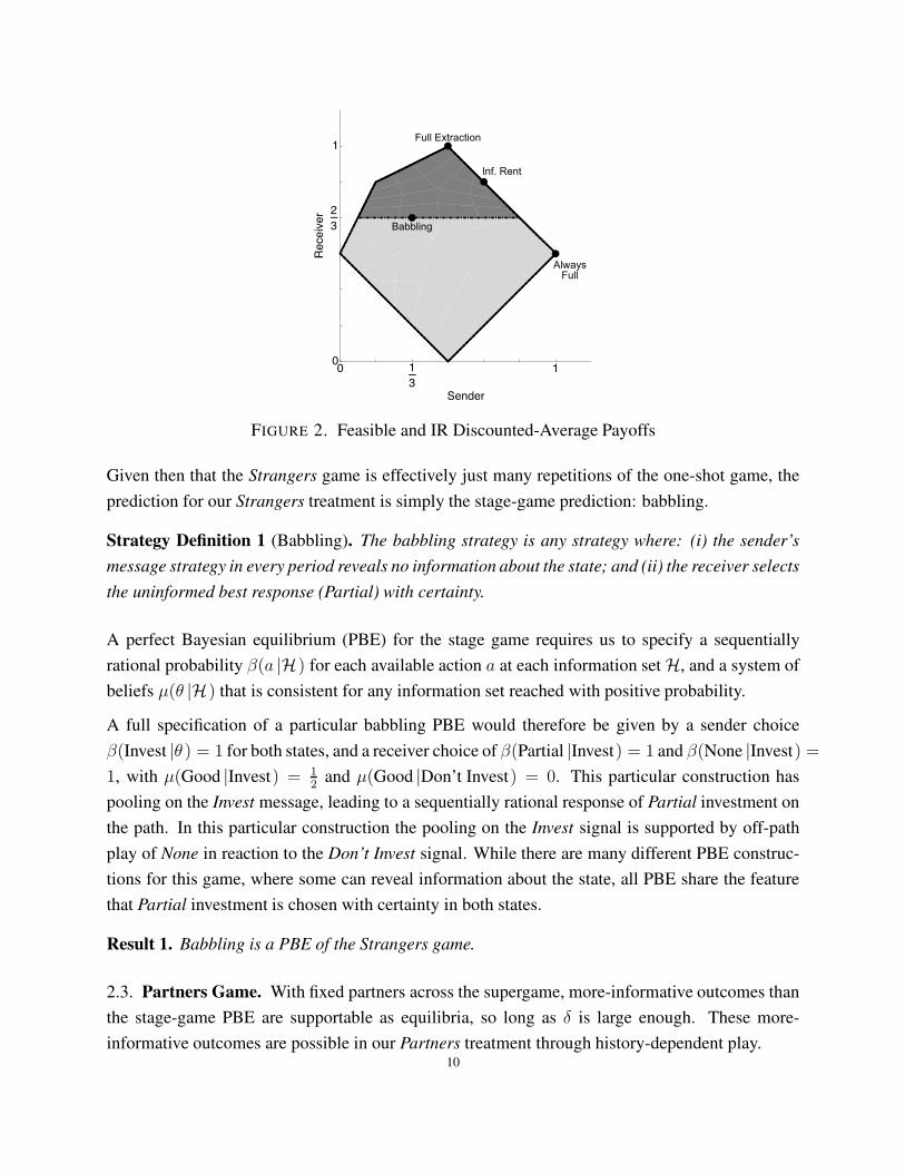
FIGURE 2. Feasible and IR Discounted-Average Payoffs

Given then that the Strangers game is effectively just many repetitions of the one-shot game, the

prediction for our Strangers treatment is simply the stage-game prediction: babbling.

Strategy Definition 1 (Babbling). The babbling strategy is any strategy where: (i) the sender’s

message strategy in every period reveals no information about the state; and (ii) the receiver selects

the uninformed best response (Partial) with certainty.

A perfect Bayesian equilibrium (PBE) for the stage game requires us to specify a sequentially

rational probability β(a |H) for each available action a at each information set H, and a system of

beliefs µ(θ |H) that is consistent for any information set reached with positive probability.

A full specification of a particular babbling PBE would therefore be given by a sender choice

β(Invest |θ ) = 1 for both states, and a receiver choice of β(Partial |Invest) = 1 and β(None |Invest) =

1, with µ(Good |Invest) = 12

and µ(Good |Don’t Invest) = 0. This particular construction has

pooling on the Invest message, leading to a sequentially rational response of Partial investment on

the path. In this particular construction the pooling on the Invest signal is supported by off-path

play of None in reaction to the Don’t Invest signal. While there are many different PBE construc-

tions for this game, where some can reveal information about the state, all PBE share the feature

that Partial investment is chosen with certainty in both states.

Result 1. Babbling is a PBE of the Strangers game.

2.3. Partners Game. With fixed partners across the supergame, more-informative outcomes than

the stage-game PBE are supportable as equilibria, so long as δ is large enough. These more-

informative outcomes are possible in our Partners treatment through history-dependent play.10

Figure 2 shows the set of feasible and individually rational expected payoffs for our stage game.

The set of feasible payoffs is indicated by the entire shaded region, while the darker gray region is

the set of individually rational payoffs. The efficient frontier of the figure runs from the extreme

point (1/2, 1), labeled Full Extraction, to the extreme point (1, 1/2), labeled Always Invest. A par-

ticular outcome lies on the efficient frontier in our game if and only if the outcome has the receiver

fully invests with certainty when the state is good. Investment behavior in the bad state defines the

locus of points that trace out the frontier, where our constant-sum restriction leads to the one for

one downward gradient.

At the leftmost extreme point on the frontier we have full extraction by the receiver. That is, this is

the payoff that would result if a fully informed receiver maximized their own payoff (fully extracted

the surplus), by choosing full investment in the good state and no investment in the bad state. At

the other extreme of the frontier is the sender’s most-preferred outcome, which is produced by the

receiver fully investing with certainty in both the good and bad state, hence the label Always Invest.

Away from the frontier, the figure illustrates the payoffs from the stage game’s babbling outcome,

at the point (1/3, 2/3). Babbling, which guarantees the receiver their individually rational payoff,

remains a PBE of the Partners game. Of note in the figure is that while the receiver’s individ-

ually rational payoff is equal to the babbling payoff, the sender’s individually rational payoff is

smaller. This is so because the receiver can enforce a payoff of zero on the sender by choosing no

investment, where the sender can be forced towards her minimal payoff without any requirement

on further revelation. As such, the worst-case individually rational payoff pair for both players is

given by the point (1/12, 2/3).16

With fixed pairs, history-dependent strategies can be used to support more-efficient outcomes so

long as δ is large enough, and standard folk-theorem constructions can be used to support continu-

ation values from the set of individually rational payoffs. In fact, given a public randomization de-

vice, all payoffs in the individually rational set are attainable as equilibria for δ = 3/4.17 Restricting

to simple pure-strategy outcomes, an inefficient, stationary PBE exists—the babbling equilibrium.

However, in addition to the babbling equilibrium, we now focus on characterizing two forms of

history-dependent equilibria for δ = 3/4: i) Equilibria with full revelation by the sender and full

extraction by the receiver; and ii) Equilibria with full revelation but without full extraction.

Full revelation-Full extraction. Full-revelation requires the sender to reveal the state at every in-

formation set along the path of play (appealing to natural language, by sending the message Invest

in the Good state and Don’t Invest in the Bad state). Full-extraction requires that the receiver

16This payoff is obtainable through a fully informed receiver choosing no investment when the state is bad, andrandomizing equally between no and partial investment when the state is good.17This was verified with the Java tool “rgsolve” (Katzwer, 2013), which uses the Abreu and Sannikov (2014) algorithmto examine the stage-game in normal form.

11

maximizes given their consistent beliefs (choosing Full investment on Invest, and None on Don’t

Invest). As the restriction fully pins down the path we turn to how this outcome can be supported

off the path. One natural candidate to supporting full extraction is reversion to babbling.

Strategy Definition 2 (Full extraction with babbling reversion). The strategy has two phases:

Full extraction: The sender fully reveals the state, the receiver fully extracts.

Punishment: Both players follow the babbling strategy.

The game starts in the Full extraction phase and remains there as long as there are no deviations.

Upon any deviation, the game moves to the punishment phase.

However, for the parameters of the game, the Full extraction-babbling strategy is not part of a PBE

of the Partners game, as the babbling outcome is not a harsh enough punishment to incentivize

senders to reveal the state.

Result 2. For δ = 34, the Full extraction-babbling strategy is not a PBE of the Partners game.

If both agents follow the Full extraction-babbling strategy, the discounted-average payoff on the

path of play is (1/2, 1). For the strategy to satisfy the one-shot deviation principle it must be that a

sender observing at θ =Bad does not want to deviate. Given that a deviation yields a static benefit

of 1 in period t instead of 0, for the deviation to be unprofitable the sender’s continuation value U⋆

under the punishment must satisfy:

(1) (1− δ) · 0 + δ · 12≥ (1− δ) · 1 + δU⋆.

So for δ = 3/4 we require that U⋆ ≤ 1/6. The babbling equilibrium is clearly too high, as UB = 1/2,

and so a harsher punishment is required to support full extraction.

The fact that reversion to babbling cannot be used to support full extraction ends up being a general

feature of these games under a fairly standard concavity assumption.18

Proposition. Consider a sender-receiver game with a continuous state space Θ = [0, 1], with the

corresponding message and action spaces M = A = [0, 1]. If the sender has a state-independent

preference u(a) increasing in a, and the receiver has a concave payoff vR(θ, a) maximized at a = θ

then full extraction can not be supported by babbling reversion for any δ ∈ (0, 1).

Proof. Full extraction (FE) requires a = θ along the path by definition, so the sender’s expected

continuation payoff on the path is uFE = Eu(θ). In the babbling outcome the receiver chooses

18The below proposition shows that full extraction can not be supported by babbling reversion when payoffs areconcave. In our specific parametrization—and setting Partial investment to be the exact intermediate between full andno investment—the sender’s payoff can be thought of as being convex over the action, 1/2 ·uS(Full)+1/2 ·uS(None) >uS(Partial). However, the result holds in our parametrization as δ = 3

4.

12

a = Eθ with certainty, so the sender’s babbling payoff is uB = u(Eθ). In any state θ < 1 the

sender strictly gains from a deviation: signaling θ = 1 (possible by full revelation) increases the

current outcome, while the change in continuation also provides a benefit (uFE ≤ uB by Jensen’s

inequality). The result therefore holds for all values of δ. �

Reversion to babbling cannot be used to support full extraction whenever payoffs are concave,

or alternatively whenever δ is small enough.19 This is not to say that harsher punishments than

babbling cannot sustain fully extractive outcomes. For a harsher punishment, the receiver could

choose zero investment for a number of periods, thus pushing the sender’s payoff towards zero.

In order for this to happen the receiver needs to take actions that give him a temporarily lower

payoff than his individually rational payoff (in our game the None action, which has an ex ante

expectation of 1/2 to the receiver). In order for this action to be rational for the receiver, it must be

that after a number of periods of this punishment, the game must eventually return to a point that

gives the receiver more than his babbling payoff. As a corollary to our proposition we therefore

have the following:

Corollary. Full extraction is only supportable as a PBE with strategies that punish the sender

more than the babbling outcome. Such punishments require receivers to at least temporarily take

outcomes which are myopically sub-optimal, and where the punishment path must at some point

returns to greater revelation than babbling.

The above points out the necessary components of punishments capable of supporting full extrac-

tion when babbling reversion does not. In terms of Figure 2, an individually rational punishment

payoff to the left of the babbling outcome must be selected. But all such points are generated

by combinations of play where the receiver has a myopic loss and where more-information than

babbling is revealed.

While fully extractive outcomes are possible in equilibrium using pure-strategies, there are two

reasons to be concerned about the predictive power of such constructions. First, such outcomes

will rely on coordination over relatively sophisticated punishments. Second, typical pure-strategy

constructions will rely on the receiver punishing across a number of periods (for instance, through

the None action) reducing his period payoff below the individually rational one. For such pun-

ishments to be incentive compatible for the receiver, an eventual return to revelation is required.

Supporting full extraction therefore necessitates the “forgiveness” of senders who have acted dis-

honestly and who have been harshly punished.

19In games where the sender has a state-dependent payoff with a bias term b > 0, even with a convex loss functionthere will typically be an upper bound δ(b) < 1 for the result, where for δ > δ(b) the game will admit fully extractiveoutcomes supported by babbling reversion.

13

While the above talks to the behavioral forces arrayed against the selection of full extraction, it is

theoretically supportable as an equilibrium in our game.

Result 3. For δ = 34, the Fully Extractive path is supportable with harsher punishments than

babbling.

This result can be demonstrated by construction. For our parametrization there are punishments

that support full extraction where the receiver chooses K1 rounds of None, followed by K2 rounds

of Partial investment followed by a return to the fully extractive path.20

Full revelation-Information rent. Above we showed that for the receiver to extract all of the sur-

plus generated by full revelation, the punishments must be more-severe and more-complex than

reversion to babbling. However, fully informative equilibria do exist where revelation is supported

by a babbling triggers. In these efficient PBE the receiver shares the generated surplus with the

sender, despite being fully informed in the bad state. As such, the payoff path lies to the right of

the fully extractive point on the efficient frontier of Figure 2. We will refer to the distance to the

right of full-extraction as the “information rent” being given to the sender.

While there are many possible efficient information rent equilibria, we focus here on the below

construction, a simple pure-strategy PBE.

Strategy Definition 3 (Information rent with babbling-trigger.). The strategy has two phases:

Information-Rent: The sender fully revels the state, the receiver selects “Full” when θ =Good

and “Partial” when θ =Bad.

Punishment: Babbling strategy.

The game starts in the information-rent phase and remains there as long as there are no deviations.

Upon any deviation, the game moves to the punishment phase, where it remains.

The expected on-path payoffs from the Information rent-babbling strategy are illustrated in Figure

2 at the point (2/3, 5/6), labeled as the Information rent outcome. The strategy provides the sender

with an expected rent of 1/6 per period, transferred as an additional payment of 1/3 in each bad-state

realization, period relative to the receiver’s myopic sequentially rational response. The outcome

doubles the sender’s payoff relative to babbling, while increasing the receiver’s payoff by 25 per-

cent.21 For the strategy to be supported as an equilibrium we need to construct punishment phase

20The (K1,K2) punishment strategy is a PBE of the Partners game for (K1,K2) ∈ {(2, 4), (2, 5), (2, 6), (3, 2), (3, 3)}21Moreover, the receiver’s revenue stream (a 1 or 2/3 each period) stochastically dominates the stream under babbling(2/3 each period).

14

payoffs (U⋆, V ⋆) on any observed deviation. To satisfy the one-shot deviation principle it is neces-

sary that neither the sender or receiver wish to deviate, which leads to the following requirements

on the punishment continuation payoffs (U⋆, V ⋆) :

(1− δ) · 13+ δ · 2

3≥ (1− δ) · 1 + δ · U⋆ ⇒ U⋆ ≤ 4

9,

(1− δ) · 23+ δ · 5

6≥ (1− δ) · 1 + δ · V ⋆ ⇒ V ⋆ ≤ 13

18

This simple outcome, where the receiver pays the information rent by selecting partial investment

when the state is revealed to be bad, can therefore be supported as equilibrium of the repeated

game by reversion to babbling outcome (1/3, 2/3) on any deviation.

Result 4. For δ = 34, the Information rent with a babbling trigger is a PBE of the Partners game.

While the particular information rents equilibrium we describe is an example of a simple equi-

librium outcome supported by babbling-reversion, other efficient outcomes with information rents

for the sender—points along the efficient frontier in Figure 2—are also possible. For instance, an

informed receiver could choose some fixed sequence of partial and no investment each time the

bad state is signaled.22

The only other efficient outcome implementable with a stationary, pure strategy is for the receiver

to choose full investment in both states. This is illustrated all the way to the right of the efficient

frontier in Figure 2, at the point labeled Always Invest. However, it is clear that this payoff can

never be an equilibrium outcome of the game as the receiver gets a discounted-average payoff of1/2, below his individually rational payoff of 2/3.

2.4. Hypotheses. Comparing the predictions for the Partners and Strangers treatments, we for-

mulate the following hypotheses.

Hypothesis 1. Information transmission in the Partners game should be equal to or higher than

in the Strangers game. Outcomes in the Partners game should be at least as efficient as in the

Strangers game.

In addition, the theoretical predictions indicate more-precise restrictions on behavior conditional

on selection.

Hypothesis 2. For the Partners game, if senders reveal information, one of the following must

hold:

(1) Receivers fully extract, but punish dishonesty with investment choices of None.

22There are no equilibria at δ = 3/4 supportable with babbling reversion where the receiver chooses full investmentwhen the bad state has been perfectly revealed. Full investment can only be chosen in equilibrium in the bad-state ifthe sender and receiver coordinate on less information provision.

15

(2) Dishonesty is punished by babbling reversion, but receivers provide an information rent to

senders.

Contrarily, for the Strangers treatment we expect the following:

Hypothesis 3. For the Strangers game, information rents are not paid by receivers when bad states

are revealed, and senders do not reveal information.

The above hypotheses are derived under the assumption that senders do not face a disutility from

lying. However, experimental work (for example, Gneezy, 2005) suggests that full revelation may

be observed in the Strangers game if senders have an aversion to lying. To capture this alternative

in the model we can modify the preferences of the senders to be

uS (θ,m, a) = uS(a)− η · 1 {m 6= mθ}

where η > 0 measures the degree of the lying aversion.

If lying aversion is high enough (η > 1), the fully informative outcome is a PBE. In other words,

observing full revelation in the Strangers treatment is consistent with a large enough aversion to

lying. However, lying aversion at this level would lead to full extraction being the equilibrium

prediction for both the Partners and Strangers treatments. As a relative difference between the

treatments our above hypothesis would remain true under lying aversion.

3. STRANGERS AND PARTNERS TREATMENTS

For both the Strangers and Partners treatments we recruited a total of 46 subjects across three

separate sessions (16, 16 and 14), and each subject participated only once.23 A session consist s

of 20 repetitions of the supergame, where each repetition involves an unknown number of periods

(δ = 3/4).24 Half of the subjects are randomly assigned to be senders and half to be receivers,

and these roles are kept fixed throughout the session. In the Strangers (Partners) treatment subjects

were randomly matched to a different participant at the beginning of each new period (supergame).

Stage-game payoffs in the laboratory are multiplied by 3, so that the bad state involves a zero-sum

23All sessions were conducted at the University of Pittsburgh and we used zTree (Fischbacher, 2007) to design ourinterface.24We randomized the length of supergames and the draws of the states prior to conducting the sessions so that thecomparison between the two treatments are balanced. Specifically, the randomization of session i of the Strangerstreatment is identical to the randomization of session i of the Partners treatment (i = 1, 2, 3). In addition, sendersin each session are matched across treatments to face an identical sequence of draws for the state θ across the entiresupergame.

16

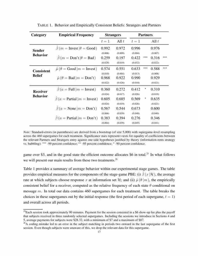
TABLE 1. Behavior and Empirically Consistent Beliefs: Strangers and Partners

Category Empirical Frequency Strangers Partners

t = 1 All t t = 1 All t

Sender

Behavior

β (m = Invest |θ = Good) 0.992 0.972 0.996 0.976(0.006) (0.009) (0.004) (0.007)

β (m = Don’t |θ = Bad) 0.259 0.197 0.422 ⋆⋆⋆ 0.316 ⋆⋆⋆

(0.029) (0.019) (0.032) (0.022)

Consistent

Belief

µ (θ = Good |m = Invest) 0.574 0.551 0.633 ⋆⋆⋆ 0.588 ⋆⋆⋆

(0.010) (0.004) (0.013) (0.008)

µ (θ = Bad |m = Don’t) 0.968 0.922 0.990 0.929(0.022) (0.026) (0.010) (0.021)

Receiver

Behavior

β (a = Full |m = Invest) 0.360 0.272 0.412 ⋆ 0.310(0.024) (0.017) (0.026) (0.019)

β (a = Partial |m = Invest) 0.605 0.685 0.569 ⋆ 0.635(0.024) (0.019) (0.026) (0.021)

β (a = None |m = Don’t) 0.567 0.544 0.673 0.600(0.066) (0.039) (0.048) (0.040)

β (a = Partial |m = Don’t) 0.383 0.394 0.276 0.346(0.064) (0.039) (0.045) (0.041)

Note: Standard-errors (in parentheses) are derived from a bootstrap (of size 5,000) with supergame-level resamplingacross the 460 supergames for each treatment. Significance stars represent t-tests for equality of coefficients betweenthe relevant Partners and Strangers entry against one-side hypotheses justified by theory (information-rents strategyvs. babbling): ⋆⋆⋆ -99 percent confidence; ⋆⋆ -95 percent confidence; ⋆ -90 percent confidence.

game over $3, and in the good state the efficient outcome allocates $6 in total.25 In what follows

we will present our main results from these two treatments.26

Table 1 provides a summary of average behavior within our experimental stage games. The table

provides empirical measures for the components of the stage-game PBE: (i) β (x |H), the average

rate at which subjects choose response x at information set H; and (ii) µ (θ |m), the empirically

consistent belief for a receiver, computed as the relative frequency of each state θ conditional on

message m. In total our data contains 460 supergames for each treatment. The table breaks the

choices in these supergames out by the initial response (the first period of each supergame, t = 1)

and overall across all periods.

25Each session took approximately 90 minutes. Payment for the session consisted in a $6 show-up fee plus the payoffthat subjects received in three randomly selected supergames. Including the sessions we introduce in Sections 4 and5, average payments for subjects were $28.32, with a minimum of $7 and a maximum of $87.26A coding mistake led to an error in the subject matching in periods two onward in the last supergame of the firstsession. Even though subjects were unaware of this, we drop the relevant data for this supergame.

17

The first set of results in Table 1 outline the sender’s strategy, where we provide the proportion of

honest (using natural language) responses after each state is realized. The first row indicates that

senders choose the Invest message in the good state at high rates. This is true in both the Strangers

and Partners treatments, particularly for the initial response where the message is selected in over

99 percent of the supergames, but for the overall response the proportion is still in excess of 97

percent for both treatments.

The strategic tension for senders arises when the state is bad, where revelation may lead to a zero

payoff. The “honest” response in the bad state is to send the message Don’t Invest, however,

our results indicate that this is not the modal message selection. In the first period of Strangers

supergames, senders select the Don’t message in reaction to a bad state in 26 percent of our data.

This declines to 20 percent when we look at all periods. For the Partners treatment the rate of

honest revelation of the bad state does increase. However, at 42 percent in the first period of each

supergame, the rate of honest revelation is not the modal response, with 58 percent of senders

instead opting for the Invest message in the bad state.

Honest revelation is not the norm in our experimental sessions. This is true for both the Strangers

and Partners treatments. For the behavior at the start of each supergame and overall. At the start

of our sessions and at the end.27,28

Though honesty is not the norm in the bad state, the message Invest still contains some information.

The next set of results in Table 1 makes precise how much information. Each entry µ is the

empirical likelihood for the matched state conditional on each message. The measure is therefore

the belief that would be consistent with the data. While the prior is 50 percent on each state, after

receiving an Invest message the good state is more likely in both treatments. At its highest point

the consistent belief indicates a 63.3 percent probability of the good state in the first period of

the Partners treatment. The expected payoff to a receiver choosing full investment is therefore

$1.89, just slightly lower than the $2.00 receivers can guarantee themselves by choosing partial

investment.

In contrast to the Invest message, given a Don’t message the probability of a corresponding bad

state is very high (99 percent in the first period of Partners’ supergames). The expected period

payoff to the receiver choosing no investment after a Don’t message is therefore $2.97 in Partners.

The high payoff from no investment following Don’t extends to the Strangers treatment with an

expected payoff of $2.77. Across both, treatments, the empirically consistent beliefs indicate that

27In the first period of the first supergame in our Partners (Strangers) treatment the message Don’t is sent followinga bad state in 33.3 (41.7) percent of our data. In contrast, the message Invest is sent 100 (100) percent of the timefollowing the good state in the very first period of the session.28Looking at the last five supergames of each session, the proportion of Don’t messages when the state is bad are 39and 23 percent for the Partners and Strangers treatments, respectively. If anything senders reveal less as the sessionproceeds.

18

receivers’ myopic best response is to choose partial investment following an Invest message and

no investment following Don’t.

The final group of results in Table 1 present the last piece of the puzzle, how receivers in our

experiments actually behave. Given three actions for each receiver information set (the Invest and

Don’t messages) we provide the proportion of choices that match the message meaning (full and

no investment, respectively) and the proportion of partial investment choices.

Receiver’s behavior in response to signals for the good state directly affect the resulting efficiency.

Choosing full investment in the good state is necessary for an efficient outcomes, but involves

trading off a certain payoff $2 against a lottery over $3 and $0, with probabilities dependent on the

belief that the sender is revealing the state.

The modal response for receivers in both Strangers and Partners mirrors the myopic best response:

partial investment in response to Invest messages, and no investment in response to Don’t Invest

messages. Though the modal response to Invest is incredulity, a large fraction of receivers do

choose to respond by investing fully. This is true for 41 percent of decisions in the first period of a

Partners supergame and 36 percent of decisions in the first period of Strangers supergames.

Though a majority of receivers respond to the Don’t message with no investment, a large minority

does choose the partial investment choice. However, examining the precise figures in Table 1,

the rate at which partial investment is chosen is higher in the Strangers treatment. That is, from

the aggregate data, subjects are more likely to make choices corresponding to the payment of an

information rent in the one-shot interactions than they are in the repeated relationship.29

The figures in the table provide evidence for the following two findings:

Finding 1. Aggregate behavior in the Stranger treatment mirrors the babbling outcome. Though

there is some honest response by a minority of senders, outcomes are not well described by the

lying-aversion prediction.

Finding 2. Aggregate behavior in our Partners treatment does show more revelation than the

Strangers treatment; however, the difference is relatively small and the modal response is still best

characterized as babbling.

To summarize, modal behavior in both treatments is better represented as babbling and the possi-

bility of using history dependent strategies in the Partners treatment appears to have only a minor

29The one-tailed tests for significance in Table 1 generated by the theory go in the opposite direction from the effect. Infact, if we were to state the opposite alternative we would be able to reject equivalence between the two treatments forreceivers choosing Partial in response to Don’t at 10 percent significance. From another point of view, the informationat the aggregate level may be misleading with respect to subjects’ strategic choices. In Appendix C we present adetailed analysis of strategies at the individual level. We do find that approximately 20% of the choices in the Partners

treatment are consistent with the Information Rent strategy, but there is no significant evidence of such strategy in theStrangers treatment.

19

effect. In Online Appendices B and C we show that indeed there are significant differences in

behavior across these two treatments in the expected direction. In particular, we do find evidence

for history dependent strategies in the Partners treatment, that is absent in the Strangers treatment.

However, though the differences between the Partners and Strangers treatments are statistically

significant—where the directions mirror the theoretical predictions (Hypothesis 1)—the sizes of

the effects are small. The previous literatures on communication and repeated play in PD games

suggested that outcomes in the Partners treatment could be highly efficient. Relative to these

priors, and the economic sizes of the effects that we find, we characterize our above findings

as a null result. Our next treatment examines the extent to which this null finding is driven by

coordination failure.

4. PRE-PLAY COMMUNICATION

One potential reason for the failure to find extensive efficiency gains in our Partners treatment

is that tacit coordination in this environment is too hard. In our environment subjects have to

coordinate on two levels. First, they need to select an equilibrium with full revelation. If the

sender does not convey the state of the world, efficiency gains are not possible. Second, they need

to solve the distributional issue that arises when information is revealed. Notice that the first trade-

off (efficient v. inefficient equilibria) is also present in a repeated PD, but the second (selecting

among efficient equilibria) is not. Moreover, notice that in selecting among efficient equilibria

two components of the strategy must be adjusted: a higher share for the receiver on-path needs

to be accompanied by a harsher punishment off-path. Difficulties in coordination at either level

may preclude subjects from reaching better outcomes. This raises the question: Would subjects in

our Partners treatment be able to achieve more-efficient outcomes if given a device to solve their

coordination problems?

To examine this question, our Chat treatment modifies the Partners repeated game to provide sub-

jects with a powerful coordination device: pre-play communication. While identical to the Part-

ners treatment for the first twelve supergames, in the last eight supergames of our Chat treatment

sessions we allow subjects to freely exchange messages through a standard chat interface.30 Re-

cruiting exactly 16 subjects for each of our three Chat sessions, we use a perfect-stranger matching

protocol in the last eight supergames with pre-play communication.31 A chat interface is available

30At the beginning of the session subjects are told that the experiment consists of two parts where Part I involves 12supergames. Only when the instructions for Part II are read (prior to supergame 13) are subjects informed that theywill be allowed to chat in the last eight supergames.31Each subject interacts with participants in the other role from them for one chat supergame only. In addition, eachnew supergame match is guaranteed to have had no previous contact with others the subject previously engaged with.The design was chosen ex ante to allow us to isolate contagion effects for particular strategies, ex post, this ended upbeing moot.

20

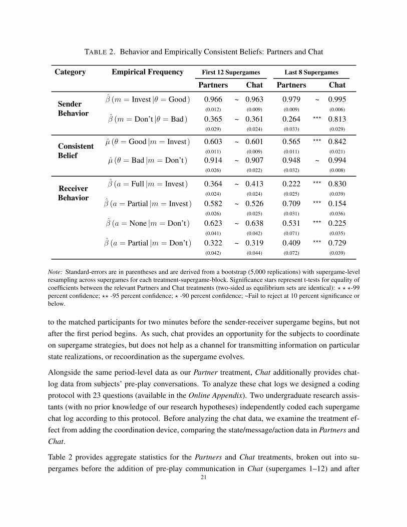
TABLE 2. Behavior and Empirically Consistent Beliefs: Partners and Chat

Category Empirical Frequency First 12 Supergames Last 8 Supergames

Partners Chat Partners Chat

Sender

Behavior

β (m = Invest |θ = Good) 0.966 ~ 0.963 0.979 ~ 0.995(0.012) (0.009) (0.009) (0.006)

β (m = Don’t |θ = Bad) 0.365 ~ 0.361 0.264 ⋆⋆⋆ 0.813(0.029) (0.024) (0.033) (0.029)

Consistent

Belief

µ (θ = Good |m = Invest) 0.603 ~ 0.601 0.565 ⋆⋆⋆ 0.842(0.011) (0.009) (0.011) (0.021)

µ (θ = Bad |m = Don’t) 0.914 ~ 0.907 0.948 ~ 0.994(0.026) (0.022) (0.032) (0.008)

Receiver

Behavior

β (a = Full |m = Invest) 0.364 ~ 0.413 0.222 ⋆⋆⋆ 0.830(0.024) (0.024) (0.025) (0.039)

β (a = Partial |m = Invest) 0.582 ~ 0.526 0.709 ⋆⋆⋆ 0.154(0.026) (0.025) (0.031) (0.036)

β (a = None |m = Don’t) 0.623 ~ 0.638 0.531 ⋆⋆⋆ 0.225(0.041) (0.042) (0.071) (0.035)

β (a = Partial |m = Don’t) 0.322 ~ 0.319 0.409 ⋆⋆⋆ 0.729(0.042) (0.044) (0.072) (0.039)

Note: Standard-errors are in parentheses and are derived from a bootstrap (5,000 replications) with supergame-levelresampling across supergames for each treatment-supergame-block. Significance stars represent t-tests for equality ofcoefficients between the relevant Partners and Chat treatments (two-sided as equilibrium sets are identical): ⋆ ⋆ ⋆-99percent confidence; ⋆⋆ -95 percent confidence; ⋆ -90 percent confidence; ~Fail to reject at 10 percent significance orbelow.

to the matched participants for two minutes before the sender-receiver supergame begins, but not

after the first period begins. As such, chat provides an opportunity for the subjects to coordinate

on supergame strategies, but does not help as a channel for transmitting information on particular

state realizations, or recoordination as the supergame evolves.

Alongside the same period-level data as our Partner treatment, Chat additionally provides chat-

log data from subjects’ pre-play conversations. To analyze these chat logs we designed a coding

protocol with 23 questions (available in the Online Appendix). Two undergraduate research assis-

tants (with no prior knowledge of our research hypotheses) independently coded each supergame

chat log according to this protocol. Before analyzing the chat data, we examine the treatment ef-

fect from adding the coordination device, comparing the state/message/action data in Partners and

Chat.

Table 2 provides aggregate statistics for the Partners and Chat treatments, broken out into su-

pergames before the addition of pre-play communication in Chat (supergames 1–12) and after21

(supergames 13–20). A comparison of the two treatments for the first 12 supergames shows that

the quantitative differences are small. In addition, our analysis of the data finds little evidence for

information-rent strategies in either treatment over the first 12 supergames.32 We therefore focus

on the differences in behavior in the last eight supergames.33

Though behavior in the first 12 supergames is similar, once we provide the coordination device,

stark differences emerge between Partners and Chat (both economically and statistically signif-

icant) for the remaining eight supergames. Overall, Chat senders report the truth more than 80

percent of the time, where their honesty in the bad-state is increased by 50 percentage points

over Partners. The effect of greater honesty in the senders’ bad-state signals is that messages

indicating the good state in are more credible. This can be seen in Table 2 by examining the

µ (θ = Good |m = Invest) row, which indicates that an Invest message is 30 percentage points

more likely to correspond to a good state in Chat than Partners. Receivers’ action choices in

Chat reflect the greater information content given Invest messages, with full investment chosen 83

percent of the time in Chat, compared to just 22 percent in Partners.

The changes in behavior documented above lead to large efficiency gains when pre-play commu-

nication is available. Conditional on a good state (the efficiency state), full investment is selected

only 28.4 percent of the time in Partners compared to 86.1 percent in Chat (last eight supergames).

However, alongside the increase in efficiency, we also observe a change in the distribution of pay-

offs when a bad state is revealed. In response to Don’t Invest messages—highly correlated with the

bad state in both treatments—we observe a 30 percentage point increase in the selection of partial

investment in Chat. Given that the Don’t Invest signal leads to subsequent feedback to receivers

revealing the bad state in 99.4 percent of Chat periods, the increased selection of partial investment

is not myopically sequentially rational. Instead, as we show below with the chat data, this choice

is a direct effect of the large majority of subjects coordinating on the information-rents strategy.

Examining the coded chat data, and conservatively reporting averages only for data where the

coders agree, we find that approximately three-quarters of complete chat exchanges have the sender

and receiver explicitly discuss the path-of-play for the information-rents strategy. While punish-

ments for deviations are only explicitly addressed in approximately one out of ten exchanges,

when punishments are discussed they always refer to babbling reversion.34 As an example of a

32The Online Appendix presents an exercise that directly estimates the presence of certain strategies. We use theStrategy Frequency Estimation Method (SFEM) of Dal Bó and Fréchette (2011), which provides maximum likelihoodestimates of the frequencies for an specified set of strategies. The frequency attributed to receivers using the informa-tion rents strategy in the Partners and Chat treatments for supergames 1-12 is effectively zero, though there is evidencethat a minority of senders try to use the strategy in both treatments.33In the Online Appendix we present an analysis at the individual level that reaches the same conclusion.34We also use the SFEM to verify the presence of the information rents strategy once chat is introduced. The report inthe Online Appendix shows that a frequency of approximately 90% is attributed to this strategy.

22

chat interaction with a discussion of punishment consider the following exchange between a re-

ceiver subject (R180) and a sender subject (S18), where we have edited the exchange to match the

economic labeling in the paper:35

R180: I’ll trust you until you lie and then it’s [partial] the whole way out.

S18: Hey want to work together on this?

R180: If you click [Don’t Invest], I’ll go [Partial] so we both get something

S18: I will tell you all the honest computer decsions if you never click [None]

S18: instead when i mark [don’t] click [partial]

S18: deal?

R180: no problem

R180: deal

Though this chat is non-representative with respect to the receiver’s articulation of the punishment,

the discussion of the on-path part component is entirely representative.36

We note that the conversation quoted above, in which both subjects nearly simultaneously outline

the information-rent strategy comes from the very first supergame where subjects had the chat in-

terface. Examining the RA-coded data, we find that 50 percent of the first-instance chat exchanges

mention the information rents strategy, which grows to 86 percent by the final chat supergame.37

While some subjects learn and adapt the information rent strategy from previous interactions, the

fact that so many supergames discuss it at the very first opportunity indicates the extent to which

subjects are aware of the strategy, but require pre-play communication to coordinate on it.38

In terms of efficiency, 91 percent of partnerships that discuss the information-rents strategy have

a perfectly efficient supergame. In contrast, only 40 percent of those chats that do not discuss the

information rents strategy have fully efficient outcomes.39

Summarizing our findings from the chat treatment:

Finding 3. While aggregate behavior in the Partners treatment mirrors the Chat treatment in the

first 12 supergames, once chat is introduced large differences between the treatments emerge. The

35The experiment had a left/middle/right (L/M/R) labeling for states, messages and actions. We replace that here withour economic labeling, indicated the edit with square brackets. All other text is verbatim.36The Online Appendix contains all chat logs from our three Chat sessions.37We focus here on supergames where our two coders agree, which is 22 of 24 for both the initial and last chatsupergames.38There are no systematic differences in who initiates the discussion of this strategy: 47 percent of supergames men-tioning the information-rents strategy have the first mention by the sender, while 53 percent are initially driven by thereceiver.39For details, and evidence for statistically significant differences driven by the information rents strategy, see theappendix, where we present a Tobit regression of the supergame efficiency on features of the pre-play discussion.

23

evidence from both observed behavior in Chat and the subject exchanges is consistent with suc-

cessful coordination on the information-rents strategy driving increased efficiency.

The fact that such a large proportion of subjects explicitly discuss the information rents strategy

from the very first chat supergame, alongside the strong efficiency increase, strongly implicates

coordination failure as the cause of low efficiency in Partners. Once subjects are provided with

an explicit channel through which to coordinate they succeed, where without it they fail. The evi-

dence from our Chat treatment indicates both that the complexity of the game is not overwhelming

for subjects, and that the payoffs implemented provide enough incentive to spur coordination on

more-efficient SPE. Instead, the low efficiency outcomes in Partners can be directly attributed to a

coordination failure.

Below we introduce a further two treatments where we explore if it is possible to aid coordination

without a direct channel for strategic collusion. Removing the pre-play communication device, we

instead provide two alternative coordination devices, maintaining the same effective incentives.

Our first provides senders with a device to aid coordination on revealing the state. The second,

provides a device to help receivers coordinate on distribution.

5. STRATEGIC COORDINATION WITHOUT CHAT: TWO ALTERNATIVES

Reviewing the exchanges in Chat we examine two alternative coordination devices, testing two

hypotheses regarding what the chat allows subjects to signal. The first hypothesis is related to

difficulties in coordination that directly preclude the transmission of information. To see why,

notice first that in the absence of chat a sender would consider a bad state realization in period

one valuable with respect to coordination. In a bad state the sender can signal to the receiver

their decision to coordinate on truthful revelation. In contrast, when the first-period realization is

good, there is no way for the sender to separate from the Always Say Invest babbling strategy. In

response to Invest, the receiver may directly select Partial. A vicious circle ensues if the sender

increases their belief that the receiver is coordinate on Always Partial, choosing not to reveal

bad states in subsequent periods. The first treatment we present in this section—our Revelation

manipulation—allows senders to convey their intentions to separate in every first period.

Our second hypothesis is that coordination difficulties are concentrated on distributional chal-

lenges. From this perspective, chatting is useful as it serves to reassure senders that they will

receive rents for revealing the bad state. That is, chat serves to coordinate both parties on the strat-

egy that Partial is chosen following Don’t, despite sender and receiver knowing that this message

reveals a bad state. Without the coordination channel, senders could expect to be taken advantage

of if they reveal bad states, and so the Invest messages is sent in both states. Moreover, if receivers

do choose Partial in response to a Don’t Invest message, senders may be uncertain on whether24

the receiver is coordinating on information rents, or on a babbling outcome that chooses Partial

investment in response to both messages. The second treatment we introduce—our Distribution

manipulation—modifies the action space of the receiver to allow them to more clearly signal that

the choice to provide an information rent.

5.1. Revelation Coordination Device. In this treatment, we change the timing of the game to

utilize a strategy method for senders. Before a state is selected, senders are asked to indicate

a message choice for each possible state realization. After senders submit their state-dependent

choices (µt : {Good,Bad} → {Invest,Don’t}), the state θt is drawn for the period and the interface

sends the receiver the relevant message, mt = µt(θt). The receiver observes the message mt

realization as before and selects an action. A crucial difference is in the provided feedback: the

receiver also learns what message she would have received in the counterfactual state—that is the

receiver’s period feedback is effectively (θt, µt, at).

The manipulation is designed not to change the theoretical predictions in any substantive way, it

simply allows senders to clearly signal their strategic intention to honesty reveal in the first period,

regardless of the state’s realization. Senders who decide to reveal (not reveal) can now be identified

from the first possible instance, where in Partners this happens only in bad states.

Table 3 presents the main aggregate behavioral responses for the treatment, where we provide data

from the Partners treatment for comparison. We present the last eight supergames of each treatment

to examine the longer-run effects. As is readily observable from the table, the Revelation Device

treatment has little differences with the Partners treatment. Senders report the truth under the bad

state approximately 30 percent of the time in the manipulation, slightly above the corresponding 26

percent for the Partners treatment. Moreover, the modal receiver response to the messages Invest

and Don’t are, respectively, Partial and None. The majority of behavior in the treatment is again

in line with the babbling equilibrium, and quantitatively close to the Partners treatment across our

measures.

The manipulation does produce a small efficiency gain: Full Investment is selected in the good

state 35 percent of the time, relative to 22 percent in the Partners treatment, where this difference

is significant at the 5 percent level. While allowing for the sender to reveal their strategy regardless

of the realization of the state may lead to an increase in efficiency, the effect is relatively small. We

summarize the finding next.

Result 5 (Revelation Device). Providing senders with a device to signal their coordination on

full revelation at the end of every period does not lead to a substantial efficiency gain. Observed

behavior is close to the Partners treatment.25

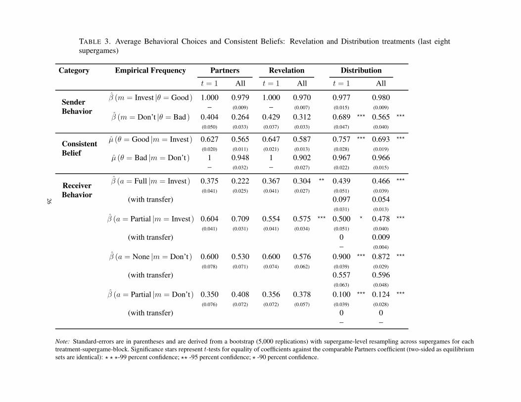
TABLE 3. Average Behavioral Choices and Consistent Beliefs: Revelation and Distribution treatments (last eightsupergames)

Category Empirical Frequency Partners Revelation Distribution

t = 1 All t = 1 All t = 1 All

Sender

Behavior

β (m = Invest |θ = Good) 1.000 0.979 1.000 0.970 0.977 0.980– (0.009) – (0.007) (0.015) (0.009)

β (m = Don’t |θ = Bad) 0.404 0.264 0.429 0.312 0.689 ⋆⋆⋆ 0.565 ⋆⋆⋆

(0.050) (0.033) (0.037) (0.033) (0.047) (0.040)

Consistent

Belief

µ (θ = Good |m = Invest) 0.627 0.565 0.647 0.587 0.757 ⋆⋆⋆ 0.693 ⋆⋆⋆

(0.020) (0.011) (0.021) (0.013) (0.028) (0.019)

µ (θ = Bad |m = Don’t) 1 0.948 1 0.902 0.967 0.966– (0.032) – (0.027) (0.022) (0.015)

Receiver

Behavior

β (a = Full |m = Invest) 0.375 0.222 0.367 0.304 ⋆⋆ 0.439 0.466 ⋆⋆⋆

(0.041) (0.025) (0.041) (0.027) (0.051) (0.039)

(with transfer) 0.097 0.054(0.031) (0.013)

β (a = Partial |m = Invest) 0.604 0.709 0.554 0.575 ⋆⋆⋆ 0.500 ⋆ 0.478 ⋆⋆⋆

(0.041) (0.031) (0.041) (0.034) (0.051) (0.040)

(with transfer) 0 0.009– (0.004)

β (a = None |m = Don’t) 0.600 0.530 0.600 0.576 0.900 ⋆⋆⋆ 0.872 ⋆⋆⋆

(0.078) (0.071) (0.074) (0.062) (0.039) (0.029)

(with transfer) 0.557 0.596(0.063) (0.048)

β (a = Partial |m = Don’t) 0.350 0.408 0.356 0.378 0.100 ⋆⋆⋆ 0.124 ⋆⋆⋆

(0.076) (0.072) (0.072) (0.057) (0.039) (0.028)

(with transfer) 0 0– –

Note: Standard-errors are in parentheses and are derived from a bootstrap (5,000 replications) with supergame-level resampling across supergames for eachtreatment-supergame-block. Significance stars represent t-tests for equality of coefficients against the comparable Partners coefficient (two-sided as equilibriumsets are identical): ⋆ ⋆ ⋆-99 percent confidence; ⋆⋆ -95 percent confidence; ⋆ -90 percent confidence.

26

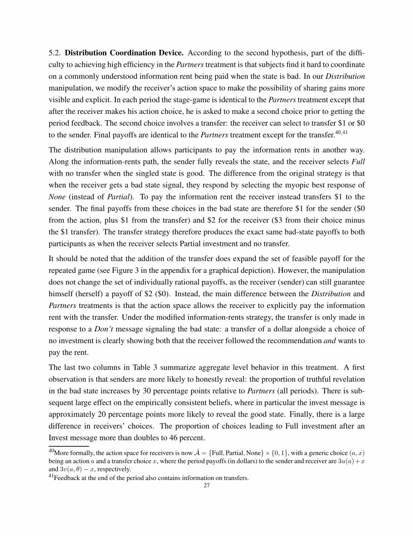
5.2. Distribution Coordination Device. According to the second hypothesis, part of the diffi-

culty to achieving high efficiency in the Partners treatment is that subjects find it hard to coordinate

on a commonly understood information rent being paid when the state is bad. In our Distribution

manipulation, we modify the receiver’s action space to make the possibility of sharing gains more

visible and explicit. In each period the stage-game is identical to the Partners treatment except that

after the receiver makes his action choice, he is asked to make a second choice prior to getting the

period feedback. The second choice involves a transfer: the receiver can select to transfer $1 or $0

to the sender. Final payoffs are identical to the Partners treatment except for the transfer.40,41

The distribution manipulation allows participants to pay the information rents in another way.

Along the information-rents path, the sender fully reveals the state, and the receiver selects Full

with no transfer when the singled state is good. The difference from the original strategy is that

when the receiver gets a bad state signal, they respond by selecting the myopic best response of

None (instead of Partial). To pay the information rent the receiver instead transfers $1 to the

sender. The final payoffs from these choices in the bad state are therefore $1 for the sender ($0

from the action, plus $1 from the transfer) and $2 for the receiver ($3 from their choice minus

the $1 transfer). The transfer strategy therefore produces the exact same bad-state payoffs to both

participants as when the receiver selects Partial investment and no transfer.

It should be noted that the addition of the transfer does expand the set of feasible payoff for the

repeated game (see Figure 3 in the appendix for a graphical depiction). However, the manipulation

does not change the set of individually rational payoffs, as the receiver (sender) can still guarantee

himself (herself) a payoff of $2 ($0). Instead, the main difference between the Distribution and

Partners treatments is that the action space allows the receiver to explicitly pay the information

rent with the transfer. Under the modified information-rents strategy, the transfer is only made in

response to a Don’t message signaling the bad state: a transfer of a dollar alongside a choice of

no investment is clearly showing both that the receiver followed the recommendation and wants to

pay the rent.

The last two columns in Table 3 summarize aggregate level behavior in this treatment. A first

observation is that senders are more likely to honestly reveal: the proportion of truthful revelation

in the bad state increases by 30 percentage points relative to Partners (all periods). There is sub-

sequent large effect on the empirically consistent beliefs, where in particular the invest message is

approximately 20 percentage points more likely to reveal the good state. Finally, there is a large

difference in receivers’ choices. The proportion of choices leading to Full investment after an

Invest message more than doubles to 46 percent.

40More formally, the action space for receivers is now A = {Full, Partial,None}×{0, 1}, with a generic choice (a, x)being an action a and a transfer choice x, where the period payoffs (in dollars) to the sender and receiver are 3u(a)+xand 3v(a, θ)− x, respectively.41Feedback at the end of the period also contains information on transfers.

27

Consistent with the information-rents equilibrium, there are very few transfers when the message

is Invest. This is shown in the row below β (a = Full |m = Invest), labeled “with transfer”, where

we provide the fraction of periods for which β (a = Full, x = $1 |m = Invest). Overall, just five

percent of choices in response to the Invest message make the $1 transfer alongside full investment,

which is approximately one-in-nine of the Full investment choices. Transfers are almost never

made (< 0.01) alongside a Partial investment choice (after either message) or alongside None after

the Invest message. However, contrasting with the very infrequent use of transfers elsewhere, we

do find that receivers do make transfers at substantial rates in exactly the situation predicted by

the modified information-rents strategy: after a Don’t Invest message alongside the No investment

action.

Relative to the Partners treatment we observe a a large increase in the choice of None follow-

ing the Don’t Invest message in the Distribution treatment (a 34 percentage point increase to 87

percent. However the large majority of these zero investment choices (68 percent) are coupled

with a $1 transfer to the sender. Pooling together the two alternative information-rent responses

(Partial/No transfer, and None/Transfer) we find that 72 percent of responses in our manipulation

pay an information rent in response to Don’t. This represents a 29.8 percent point increase over

Partners (significant at the 1 percent level). Overall, the aggregate statistics indicate that behavior

is more-consistent with the information rents equilibrium when the rent can be paid as an explicit

transfer.

Examining the ensuing efficiency: Full investment is selected for 52.1 percent of good states.

This figure represent more than double the efficiency in our Partners treatment, and approximately

60 percent of the efficiency level achieved in our chat treatment. The findings for this treatment

suggest that a simple manipulation of the receivers action-space that allows information rents to be

explicit paid achieves substantial efficiency gains and pushes the behavior towards the information-

rent equilibrium. We summarize the main finding for this treatment.

Result 6 (Explicit Rents). Modal behavior in the treatment where we provide subjects with a dis-

tributional coordination device is consistent with the information-rents equilibrium; the possibility

of an explicit transfer greatly increase efficiency over our Partners treatment.

6. CONCLUSION

Our paper examines the intersection of two important economic topics: the transfer of information,

and the use of dynamic strategies. For the transfer of information an array of behavioral forces

(lying aversion, bounded rationality) have been show to push outcomes in one-shot settings toward

greater revelation than predicted by theory. For dynamic strategies, a large experimental literature

on infinite-horizon PD games suggests that subjects readily utilizing dynamic strategies to produce28

more-efficient outcomes. However, when we combine these two forces, where honest response can

be an efficient equilibrium outcome, we do not find behavior that is substantially more efficient.

Though we find evidence that subjects in our Partners treatments are capable of responding dy-

namically to more-cooperative choices of their partners, the overwhelming coordination is on the

low-efficiency babbling outcome. Through additional treatments we show that coordination on

efficiency can be very challenging. Subjects in the informed sender role are willing to truthfully

reveal, but only when they are not punished for revealing information against their own myopic in-

terest; that is when they are provided with an information rent. While it is possible for honesty to be

compelled in equilibrium without an information rent through the (credible) threat of punishment

for any dishonesty, such punishments are strategically complex. In contrast, in our experiments the

only punishments we observe are much simpler ones: reversions to the stage game equilibrium.

Our paper, along with other work on dynamic games (see Vespa and Wilson, 2015) suggest an

empirically motivated refinement for the analysis of environments with folk theorems. Examining

just history-independent equilibria—for example, the stage-game PBE in our setting, or the MPE

in a dynamic game—will remove more-efficient equilibrium strategies that are openly articulated

and used by subjects in our experiments. While we do find evidence for simple dynamic strategies

that revert to history-independent equilibrium play on miscoordination, we find no evidence for

subjects using harsher punishments than this.

While complex punishment strategies are analytically useful in proving the extents of what a dy-

namic strategic response can do, they seem to have little predictive content. Instead, our paper

motivates behaviorally restricted folk theorems that examine what can be achieved with reversion

to the stationary equilibrium. Rather than the individually rational payoff set, the important coun-

terfactual for understanding whether an outcome can or cannot be supported dynamically is the

history-independent equilibrium outcome.

Importantly, while this restriction on punishments matches observations on behavior, the restric-

tion’s equilibrium implications of what types of outcomes can be sustained predicts our main find-

ing: information rents are necessary for more-efficient outcomes. This prediction based on simple

punishments, is borne out both in observed on path behavior and via subjects’ pre-play communi-

cation. Where subjects are not rewarded for their honesty in our experiments, they stop revealing

information. To take a complementary line from King Lear to our opening quote “Nothing comes

from nothing.”

REFERENCES

ABREU, D. AND Y. SANNIKOV (2014): “An algorithm for two-player repeated games with perfect moni-toring,” Theoretical Economics, 9, 313–338.

29

ARECHAR, A., A. DREBER, D. FUDENBERG, AND D. RAND (2016): “The role of communication innoisy repeated games,” Mimeo.

BARON, D. P. AND D. BESANKO (1984): “Regulation and information in a continuing relationship,” Infor-

mation Economics and policy, 1, 267–302.BLUME, A., D. V. DEJONG, Y.-G. KIM, AND G. B. SPRINKLE (1998): “Experimental evidence on the

evolution of meaning of messages in sender-receiver games,” American Economic Review, 88, 1323–1340.

BROWN, M., A. FALK, AND E. FEHR (2004): “Relational contracts and the nature of market interactions,”Econometrica, 72, 747–780.

CAI, H. AND J. WANG (2006): “Overcommunication in strategic information transmission games,” Games

and Economic Behavior, 56, 7–36.CAMERA, G. AND M. CASARI (2009): “Cooperation among strangers under the shadow of the future,”

American Economic Review, 99, 979–1005.COOPER, D. J. AND J. H. KAGEL (2005): “Are two heads better than one? Team versus individual play in

signaling games,” American Economic Review, 95, 477–509.CRAWFORD, V. P. AND J. SOBEL (1982): “Strategic Information Transmission,” Econometrica, 50, 1431–

1451.DAL BÓ, P. AND G. R. FRÉCHETTE (2011): “The evolution of cooperation in infinitely repeated games:

Experimental evidence,” American Economic Review, 101, 411–429.DAL BÓ, P. AND G. R. FRÉCHETTE (2016): “On the Determinants of Cooperation in Infinitely Repeated

Games: A Survey,” .DICKHAUT, J. W., K. A. MCCABE, AND A. MUKHERJI (1995): “An experimental study of strategic

information transmission,” Economic Theory, 6, 389–403.DREBER, A., D. RAND, D. FUDENBERG, AND M. NOWAK (2008): “Winners don’t punish,” Nature, 452,

348–351.DUFFY, J. AND J. OCHS (2009): “Cooperative behavior and the frequency of social interaction,” Games

and Economic Behavior, 66, 785–812.DUTTA, P. K. (1995): “A folk theorem for stochastic games,” Journal of Economic Theory, 66, 1–32.EMBREY, M., G. FRÉCHETTE, AND E. STACCHETTI (2013): “An Experimental Study of Imperfect Public

Monitoring: Efficiency versus Renegotiation-Proofness,” .ETTINGER, D. AND P. JEHIEL (2015): “An Experiment on Deception, Credibility and Trust,” UCL working

paper.FISCHBACHER, U. (2007): “z-Tree: Zurich toolbox for ready-made economic experiments,” Experimental

Economics, 10, 171–178.FISCHBACHER, U. AND F. FÖLLMI-HEUSI (2013): “Lies in disguise—an experimental study on cheating,”

Journal of the European Economic Association, 11, 525–547.FUDENBERG, D., D. LEVINE, AND E. MASKIN (1994): “The folk theorem with imperfect public informa-

tion,” Econometrica, 997–1039.FUDENBERG, D. AND E. MASKIN (1986): “The folk theorem in repeated games with discounting or with

incomplete information,” Econometrica, 533–554.FUDENBERG, D., D. RAND, AND A. DREBER (2010): “Slow to anger and fast to forgive: Cooperation in

an uncertain world,” American Economic Review.GNEEZY, U. (2005): “Deception: The Role of Consequences,” American Economic Review, 95, 384–394.GOLOSOV, M., V. SKRETA, A. TSYVINSKI, AND A. WILSON (2014): “Dynamic strategic information

transmission,” Journal of Economic Theory, 151, 304–341.HURKENS, S. AND N. KARTIK (2009): “Would I lie to you? On social preferences and lying aversion,”

Experimental Economics, 12, 180–192.KAGEL, J. H. AND P. MCGEE (2016): “Team versus Individual Play in Finitely Repeated Prisoner Dilemma

Games,” American Economic Journal: Microeconomics, 8, 253–76.

30

KATZWER, R. (2013): “rgsolve for Java,” mimeo.LAFFONT, J.-J. AND J. TIROLE (1988): “The Dynamics of Incentive Contracts,” Econometrica, 56, 1153–

75.RENAULT, J., E. SOLAN, AND N. VIEILLE (2013): “Dynamic sender–receiver games,” Journal of Eco-

nomic Theory, 148, 502–534.SOBEL, J. (1985): “A theory of credibility,” The Review of Economic Studies, 52, 557.SUTTER, M. (2009): “Deception through telling the truth?! experimental evidence from individuals and

teams,” Economic Journal, 119, 47–60.VESPA, E. (2016): “An Experimental Investigation of Strategies in Dynamic Games,” UCSB working paper.VESPA, E. AND A. J. WILSON (2015): “Experimenting with Equilibrium Selection in Dynamic Games,”

Stanford working paper.WANG, J., M. SPEZIO, AND C. F. CAMERER (2010): “Pinocchio’s Pupil: Using Eyetracking and Pupil

Dilation to Understand Truth Telling and Deception in Sender-Receiver Games,” American Economic

Review, 100, 984–1007.WILSON, A. J. AND H. WU (2016): “At-will Relationships: How an Option to Walk Away Affects Coop-

eration and Efficiency,” University of Pittsburgh working paper.

31

� �� �

�

��

�

������

��������

Babbling

FullExtraction

AlwaysFull

Inf.Rent

(A) Partners (no transfer)

� �� �

�

��

�

��������������

Babbling

FullExtraction

AlwaysFull

Inf.Rent

AlwaysFull+T

(B) Parners (with transfer)

FIGURE 3. Feasible and IR Discounted-Average Payoffs: Partners vs. Distribution

APPENDIX A. ONLINE APPENDIX: ADDITIONAL FIGURES AND TABLES

32

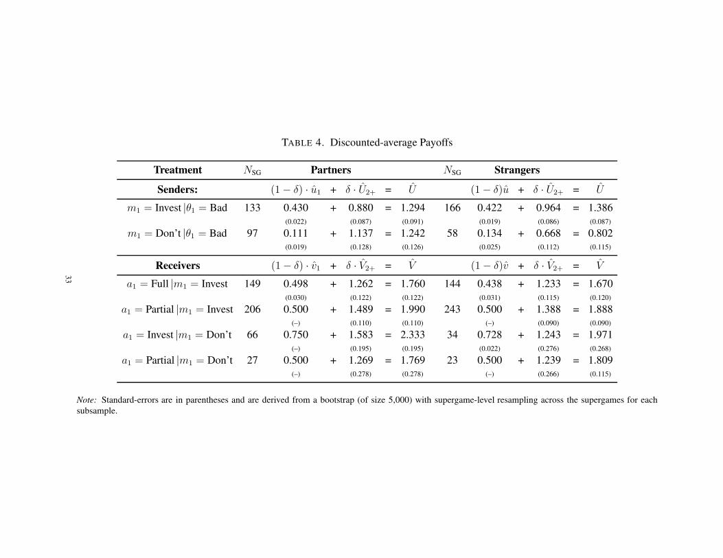
TABLE 4. Discounted-average Payoffs

Treatment NSG Partners NSG Strangers

Senders: (1− δ) · u1 + δ · U2+ = U (1− δ)u + δ · U2+ = U

m1 = Invest |θ1 = Bad 133 0.430 + 0.880 = 1.294 166 0.422 + 0.964 = 1.386(0.022) (0.087) (0.091) (0.019) (0.086) (0.087)

m1 = Don’t |θ1 = Bad 97 0.111 + 1.137 = 1.242 58 0.134 + 0.668 = 0.802(0.019) (0.128) (0.126) (0.025) (0.112) (0.115)

Receivers (1− δ) · v1 + δ · V2+ = V (1− δ)v + δ · V2+ = V

a1 = Full |m1 = Invest 149 0.498 + 1.262 = 1.760 144 0.438 + 1.233 = 1.670(0.030) (0.122) (0.122) (0.031) (0.115) (0.120)

a1 = Partial |m1 = Invest 206 0.500 + 1.489 = 1.990 243 0.500 + 1.388 = 1.888(–) (0.110) (0.110) (–) (0.090) (0.090)

a1 = Invest |m1 = Don’t 66 0.750 + 1.583 = 2.333 34 0.728 + 1.243 = 1.971(–) (0.195) (0.195) (0.022) (0.276) (0.268)

a1 = Partial |m1 = Don’t 27 0.500 + 1.269 = 1.769 23 0.500 + 1.239 = 1.809(–) (0.278) (0.278) (–) (0.266) (0.115)

Note: Standard-errors are in parentheses and are derived from a bootstrap (of size 5,000) with supergame-level resampling across the supergames for eachsubsample.

33

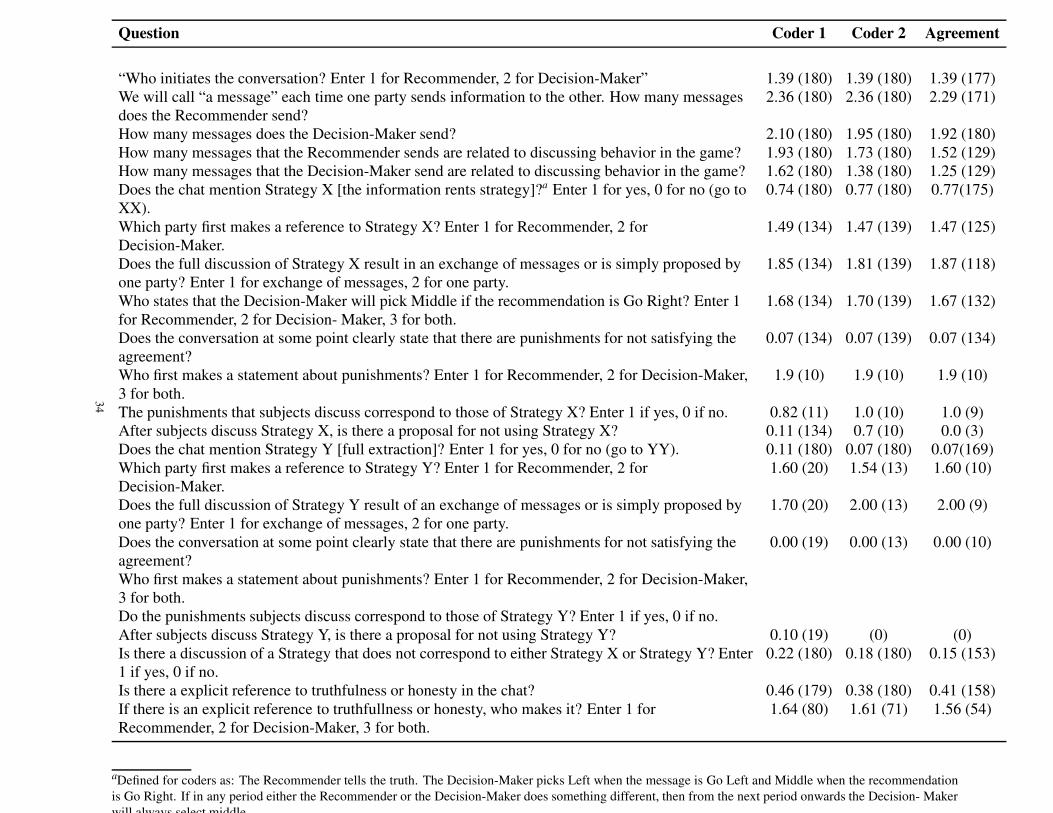
TABLE 5. Coded Chat Data

Question Coder 1 Coder 2 Agreement

“Who initiates the conversation? Enter 1 for Recommender, 2 for Decision-Maker” 1.39 (180) 1.39 (180) 1.39 (177)We will call “a message” each time one party sends information to the other. How many messagesdoes the Recommender send?

2.36 (180) 2.36 (180) 2.29 (171)

How many messages does the Decision-Maker send? 2.10 (180) 1.95 (180) 1.92 (180)How many messages that the Recommender sends are related to discussing behavior in the game? 1.93 (180) 1.73 (180) 1.52 (129)How many messages that the Decision-Maker send are related to discussing behavior in the game? 1.62 (180) 1.38 (180) 1.25 (129)Does the chat mention Strategy X [the information rents strategy]?a Enter 1 for yes, 0 for no (go toXX).

0.74 (180) 0.77 (180) 0.77(175)

Which party first makes a reference to Strategy X? Enter 1 for Recommender, 2 forDecision-Maker.

1.49 (134) 1.47 (139) 1.47 (125)

Does the full discussion of Strategy X result in an exchange of messages or is simply proposed byone party? Enter 1 for exchange of messages, 2 for one party.

1.85 (134) 1.81 (139) 1.87 (118)

Who states that the Decision-Maker will pick Middle if the recommendation is Go Right? Enter 1for Recommender, 2 for Decision- Maker, 3 for both.

1.68 (134) 1.70 (139) 1.67 (132)

Does the conversation at some point clearly state that there are punishments for not satisfying theagreement?

0.07 (134) 0.07 (139) 0.07 (134)

Who first makes a statement about punishments? Enter 1 for Recommender, 2 for Decision-Maker,3 for both.

1.9 (10) 1.9 (10) 1.9 (10)

The punishments that subjects discuss correspond to those of Strategy X? Enter 1 if yes, 0 if no. 0.82 (11) 1.0 (10) 1.0 (9)After subjects discuss Strategy X, is there a proposal for not using Strategy X? 0.11 (134) 0.7 (10) 0.0 (3)Does the chat mention Strategy Y [full extraction]? Enter 1 for yes, 0 for no (go to YY). 0.11 (180) 0.07 (180) 0.07(169)Which party first makes a reference to Strategy Y? Enter 1 for Recommender, 2 forDecision-Maker.

1.60 (20) 1.54 (13) 1.60 (10)

Does the full discussion of Strategy Y result of an exchange of messages or is simply proposed byone party? Enter 1 for exchange of messages, 2 for one party.

1.70 (20) 2.00 (13) 2.00 (9)

Does the conversation at some point clearly state that there are punishments for not satisfying theagreement?

0.00 (19) 0.00 (13) 0.00 (10)

Who first makes a statement about punishments? Enter 1 for Recommender, 2 for Decision-Maker,3 for both.Do the punishments subjects discuss correspond to those of Strategy Y? Enter 1 if yes, 0 if no.After subjects discuss Strategy Y, is there a proposal for not using Strategy Y? 0.10 (19) (0) (0)Is there a discussion of a Strategy that does not correspond to either Strategy X or Strategy Y? Enter1 if yes, 0 if no.

0.22 (180) 0.18 (180) 0.15 (153)

Is there a explicit reference to truthfulness or honesty in the chat? 0.46 (179) 0.38 (180) 0.41 (158)If there is an explicit reference to truthfullness or honesty, who makes it? Enter 1 forRecommender, 2 for Decision-Maker, 3 for both.

1.64 (80) 1.61 (71) 1.56 (54)

aDefined for coders as: The Recommender tells the truth. The Decision-Maker picks Left when the message is Go Left and Middle when the recommendationis Go Right. If in any period either the Recommender or the Decision-Maker does something different, then from the next period onwards the Decision- Makerwill always select middle.

34

TABLE 6. Tobit Regression on Supergame Efficiency

Variable Coeff. Std. Err Marginal Effect Std. Err

Mention Information Rents strategy 1.903 ⋆⋆⋆ 0.637 0.505 ⋆⋆ 0.204Mention Full Extraction strategy 0.206 0.683 0.067 0.219

Mention Other Strategy 0.790 0.624 0.256 0.200Supergame Number 0.0127 0.084 0.002 0.027

Constant 0.705 0.544 0.404 ⋆⋆ 0.179

Note: The Tobit regression examines the subsample of 192 chat supergames for 118 supergames with: i) One or more rounds in the good state, which eliminates42 supergames); and ii) perfect agreement between the two chat coders, which eliminates 43 supergames, 11 overlapping with condition (i). The Tobit controlsfor censoring at an efficiency level of 100 percent, as 102 of the 118 supergames are perfectly efficient. Marginal effects are the change in probability (baseprobability for the constant) of achieving a perfectly efficient supergame (the censored region for the Tobit) as each variable shifts from 0 to 1. Standard errorsfor the marginal effects calculated using the delta method.

35

APPENDIX B. ONLINE APPENDIX: ANALYSIS AT THE AGGREGATE LEVEL

In this section we provide statistical support for the statements in Sections 3, 4 and 5. We now

describe the approach that we follow to compare across treatments. In the case of senders, the

vast majority of messages are to Invest when the state is good, so the informative comparisons

take place when the state is bad, so we therefore focus our analysis on these cases. The dependent

variable in the analysis is a dummy that takes value 1 if the subject sent the message Invest and 0

otherwise. On the right-hand-side we have a treatment dummy (to be specified in each comparison)

and a constant.

For receivers, we conduct two separate sets of regressions. First, we consider the case when the

message is Invest. When such message is received, the informative comparison is to evaluate if

the receiver decides to fully invest or not. Hence, we define the dependent variable in this case

as 1 if the receiver fully invests and 0 otherwise. Second, consider the case when the message is

Don’t Invest. In this case, we want to evaluate if the receiver selects Partial or not. Hence, our

dependent variable in this case is a dummy variable that takes value 1 if the receiver’s action is

Partial and 0 otherwise. In each case we report the estimates on the right-hand-side decision using

a random-effects linear probability model.42

Table 7 reports the results for a comparison of the Partners and the Strangers treatment, with

the treatment dummy (Parters) taking value 1 (0) if the observation comes from the Partners

(Strangers) treatment. In each case we present the output including all supergames (All S) and

also constrained to the last eight supergames (S > 12). The findings are in line with the test of

proportion we report in the text: there are basically no statistical differences at the aggregate level

between the Partners and the Strangers treatment either with respect to the behavior of Senders or

Receivers. In the next appendix section we show, however, that there are small differences across

these two treatments when we condition on past play.

Table 8 presents the comparison between the Chat and Partners treatments, with the treatment

dummy (Chat) taking value 1 (0) if the observation comes from the Chat (Partners) treatment. The

table presents the output for supergames prior to the introduction of pre-play communication (S ≤

12) and supergames with pre-play communication (S > 12). There is no statistical differences

across treatments prior to the introduction of pre-play communication, but there are large and

statistically significant treatment effects once chat is introduced in all cases. For senders, in the

last eight supergames, we find a negative treatment effect, which means that subjects are less likely

to dishonestly send the message Invest in the bad state. Meanwhile, we find that receivers are

much more likely to follow the sender’s recommendation when the message is Invest. In this case,

42We decided to report a linear probability model for ease of presentation. The results are qualitatively similar if weestimate a random effects probit model for the senders or an random effects ordered probit for receivers (given thatreceivers are deciding among three ordered options).

36

subjects in the Chat treatment select Full significantly more often than in Partners. On the other

hand, when the message is Don’t Invest, receiver subjects in the Chat treatment are much more

likely to select Partial investment, consistent with the information-rents strategy.

Table 9 displays the output for the comparison between the Revelation and Partners treatments,

with the treatment dummy (Revelation) taking value 1 (0) if the observation comes from the Reve-

lation (Partners) treatment. We present results for all supergames and for the last eight supergames

in each case. We basically find that there is no significant treatment effect relative to Partners.

Moreover, the estimates for the treatment dummy are quantitatively small .

Finally, Table 10 shows the output for the comparison between the Distribution treatment (with

the treatment dummy Distribution taking value 1) and the Partners treatment (with the treatment

dummy taking value 0). In this case we do find differences in behavior for senders and receivers.

In the case of senders we find that subjects are more likely to tell the truth in the Distribution treat-

ment. The increase of truth-telling is between 20 and 30 percentage points. We find a significant

effect for receivers when the message is invest if we focus on all periods. The treatment effect

involves an increase between 11 and 21 percentage points. Finally, in all cases we find a difference

in choices when the message is Don’t Invest. In this case, subjects are more less likely to choose

Partial in the Distribution treatment. The reason for this is that receivers are choosing None much

more often (but are instead opting to make an explicit transfer).

37

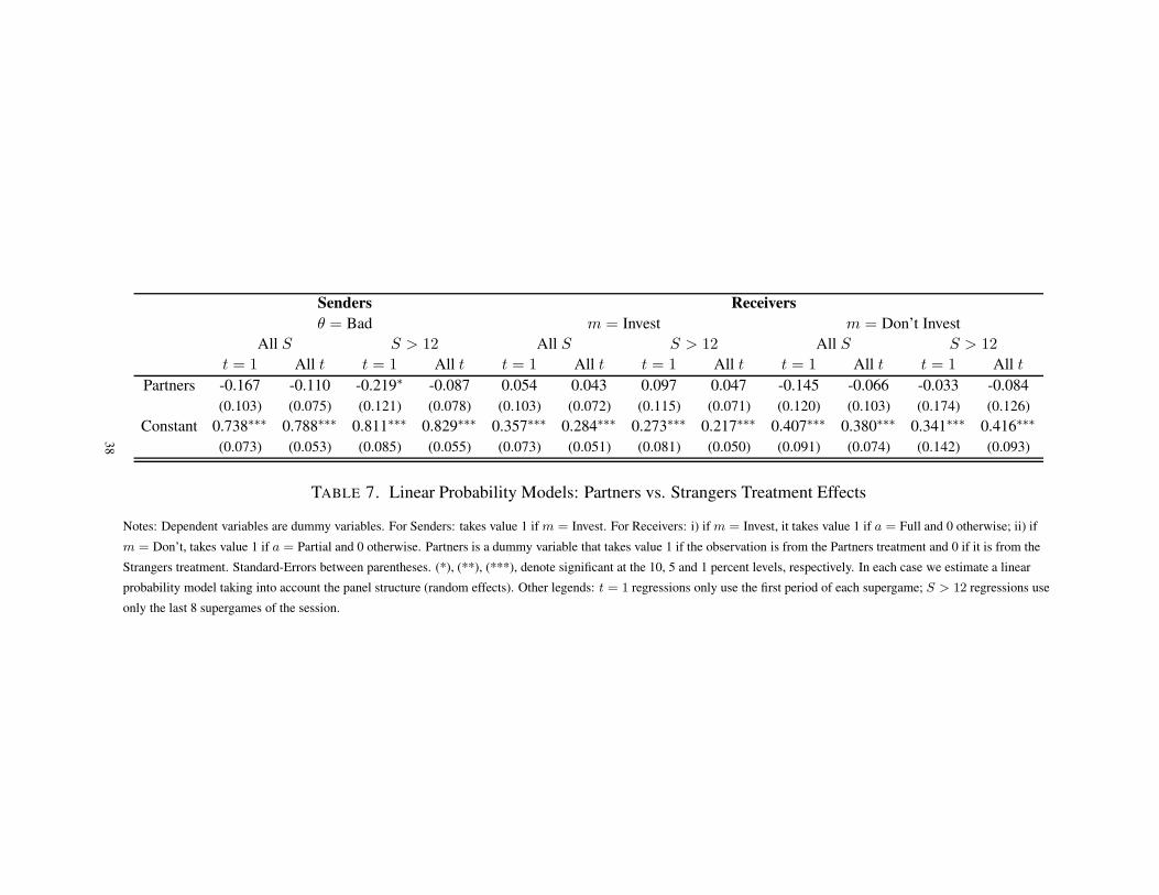
Senders Receivers

θ = Bad m = Invest m = Don’t InvestAll S S > 12 All S S > 12 All S S > 12

t = 1 All t t = 1 All t t = 1 All t t = 1 All t t = 1 All t t = 1 All tPartners -0.167 -0.110 -0.219∗ -0.087 0.054 0.043 0.097 0.047 -0.145 -0.066 -0.033 -0.084

(0.103) (0.075) (0.121) (0.078) (0.103) (0.072) (0.115) (0.071) (0.120) (0.103) (0.174) (0.126)

Constant 0.738∗∗∗ 0.788∗∗∗ 0.811∗∗∗ 0.829∗∗∗ 0.357∗∗∗ 0.284∗∗∗ 0.273∗∗∗ 0.217∗∗∗ 0.407∗∗∗ 0.380∗∗∗ 0.341∗∗∗ 0.416∗∗∗

(0.073) (0.053) (0.085) (0.055) (0.073) (0.051) (0.081) (0.050) (0.091) (0.074) (0.142) (0.093)

TABLE 7. Linear Probability Models: Partners vs. Strangers Treatment Effects

Notes: Dependent variables are dummy variables. For Senders: takes value 1 if m = Invest. For Receivers: i) if m = Invest, it takes value 1 if a = Full and 0 otherwise; ii) if

m = Don’t, takes value 1 if a = Partial and 0 otherwise. Partners is a dummy variable that takes value 1 if the observation is from the Partners treatment and 0 if it is from the

Strangers treatment. Standard-Errors between parentheses. (*), (**), (***), denote significant at the 10, 5 and 1 percent levels, respectively. In each case we estimate a linear

probability model taking into account the panel structure (random effects). Other legends: t = 1 regressions only use the first period of each supergame; S > 12 regressions use

only the last 8 supergames of the session.

38

Senders Receivers

θ = Bad m = Invest m = Don’t InvestS ≤ 12 S > 12 S ≤ 12 S > 12 S ≤ 12 S > 12

t = 1 All t t = 1 All t t = 1 All t t = 1 All t t = 1 All t t = 1 All tChat 0.058 0.020 -0.438∗∗∗ -0.555∗∗∗ 0.028 0.027 0.501∗∗∗ 0.574∗∗∗ 0.062 -0.018 0.403∗∗∗ 0.378∗∗∗

(0.097) (0.072) (0.112) (0.074) (0.108) (0.072) (0.100) (0.070) (0.121) (0.100) (0.113) (0.099)

Constant 0.561∗∗∗ 0.619∗∗∗ 0.592∗∗∗ 0.742∗∗∗ 0.443∗∗∗ 0.384∗∗∗ 0.370∗∗∗ 0.265∗∗∗ 0.223∗∗∗ 0.303∗∗∗ 0.322∗∗∗ 0.338∗∗∗

(0.069) (0.051) (0.080) (0.053) (0.077) (0.051) (0.071) (0.050) (0.086) (0.071) (0.087) (0.075)

TABLE 8. Linear Probability Models: Chat vs. Partners Treatment Effects

Notes: Dependent variables are dummy variables. For Senders: takes value 1 if m = Invest. For Receivers: i) if m = Invest, it takes value 1 if a = Full and 0 otherwise; ii) if

m = Don’t, takes value 1 if a = Partial and 0 otherwise. Chat is a dummy variable that takes value 1 if the observation is from the Chat treatment and 0 if it is from the Partners

treatment. Standard-Errors between parentheses. (*), (**), (***), denote significant at the 10, 5 and 1 percent levels, respectively. In each case we estimate a linear probability

model taking into account the panel structure (random effects). Other legends: t = 1 regressions only use the first period of each supergame; S > 12 regressions use only the last

8 supergames of the session.

39

Senders Receivers

θ = Bad m = Invest m = Don’t InvestAll S S > 12 All S S > 12 All S S > 12

t = 1 All t t = 1 All t t = 1 All t t = 1 All t t = 1 All t t = 1 All tRevelation 0.017 -0.036 -0.019 -0.093 -0.018 0.026 0.013 0.062 -0.145 -0.066 -0.033 -0.084

(0.113) (0.084) (0.138) (0.093) (0.103) (0.066) (0.123) (0.074) (0.120) (0.103) (0.174) (0.126)

Constant 0.571∗∗∗ 0.677∗∗∗ 0.592∗∗∗ 0.742∗∗∗ 0.411∗∗∗ 0.326∗∗∗ 0.369∗∗∗ 0.264∗∗∗ 0.407∗∗∗ 0.380∗∗∗ 0.341∗∗∗ 0.416∗∗∗

(0.080) (0.059) (0.098) (0.065) (0.072) (0.047) (0.086) (0.052) (0.091) (0.074) (0.142) (0.093)

TABLE 9. Linear Probability Models: Revelation Device vs. Partners Treatment Effects

Notes: Dependent variables are dummy variables. For Senders: takes value 1 if m = Invest. For Receivers: i) if m = Invest, it takes value 1 if a = Full and 0 otherwise; ii) if

m = Don’t, takes value 1 if a = Partial and 0 otherwise. Revelation Device is a dummy variable that takes value 1 if the observation is from the Revelation treatment and 0 if it

is from the Partners treatment. Standard-Errors between parentheses. (*), (**), (***), denote significant at the 10, 5 and 1 percent levels, respectively. In each case we estimate a

linear probability model taking into account the panel structure (random effects). Other legends: t = 1 regressions only use the first period of each supergame; S > 12

regressions use only the last 8 supergames of the session.

40

Senders Receivers

θ = Bad m = Invest m = Don’t InvestAll S S > 12 All S S > 12 All S S > 12

t = 1 All t t = 1 All t t = 1 All t t = 1 All t t = 1 All t t = 1 All tDistribution -0.214∗∗ -0.205∗∗ -0.254∗ -0.284∗∗∗ 0.129 0.167∗∗ 0.114 0.214∗∗ -0.168∗∗ -0.186∗∗ -0.230∗∗ -0.213∗∗

(0.109) (0.080) (0.135) (0.089) (0.112) (0.079) (0.130) (0.091) (0.082) (0.078) (0.100) (0.091)

Constant 0.571∗∗∗ 0.678∗∗∗ 0.592∗∗∗ 0.742∗∗∗ 0.411∗∗∗ 0.326∗∗∗ 0.369∗∗∗ 0.265∗∗∗ 0.264∗∗∗ 0.314∗∗∗ 0.316∗∗∗ 0.334∗∗∗

(0.077) (0.057) (0.096) (0.065) (0.079) (0.047) (0.091) (0.064) (0.060) (0.056) (0.074) (0.066)

TABLE 10. Linear Probability Models: Distribution vs. Partners Treatment Effects

Notes: Dependent variables are dummy variables. For Senders: takes value 1 if m = Invest. For Receivers: i) if m = Invest, it takes value 1 if a = Full and 0 otherwise; ii) if

m = Don’t, takes value 1 if a = Partial and 0 otherwise. Distribution Device is a dummy variable that takes value 1 if the observation is from the Distribution treatment and 0 if

it is from the Partners treatment. Standard-Errors between parentheses. (*), (**), (***), denote significant at the 10, 5 and 1 percent levels, respectively. In each case we estimate

a linear probability model taking into account the panel structure (random effects). Other legends: t = 1 regressions only use the first period of each supergame; S > 12

regressions use only the last 8 supergames of the session.

41

APPENDIX C. ONLINE APPENDIX: HISTORY DEPENDENCE

Analysis at the aggregate level. Though the overall data indicates a modal response that exactly

reflects the babbling outcome, we now show that subjects in our Partners treatment do react to

history within the supergame. Table 11 presents aggregate evidence that subjects respond to history

in the Partners treatment but not in Strangers. To define the dependent variables for senders and

receivers we follow a similar approach as described in Appendix B: For senders we focus on cases

when the state is bad and the dependent variable equals one if the subject recommends Invest. For

receivers we distinguish based on the current message. If the message is Invest, the dependent

variable takes value 1 if the subject chooses Full investment and 0 otherwise. If the message is

Don’t Invest, the dependent variable takes value 1 if the subject chooses Partial and 0 otherwise.

We present results for all supergames and for the the last eight. In addition, in each case we

distinguish between a sample that includes only the second period (after there is a single period of

previous history, we label these regressions as “t = 2”) and all periods after the first (“t ≥ 2”).

On the right-hand side we include three control variables. A treatment dummy that takes value

1 if the observation is from Partners. An Information Rents feedback dummy: i) for senders it

takes value 1 if in the previous period the message was Invest and the receiver selected Full, or

if the message was Don’t Invest and the receiver selected Partial; ii) for receivers it takes value 1

if the sender’s message was truthful in the previous period. In other words the dummy captures

cases where the outcome last period was ‘positive’, and we would expect a reaction to past play

after such positive events. Finally, we also include the interaction between the Information Rents

feedback and Partners treatment dummy.

The main finding in the table is that the interaction dummy is always significant for senders and it

is significant for receivers after Invest messages. This indicates, that senders are significantly more

likely to respond by telling the truth in the current period if the feedback last period was positive

and they are participating in Partners. Meanwhile there is no effect on truth-telling after positive

feedback to senders in the Strangers treatment.

In the case of receivers, we document no significant effect of past play on choices in a round with

a Don’t Invest message, receiver subjects in both Strangers and Partners react similarly. However,

there is a treatment effect for receivers when the message is Invest. In this case, subjects are more

likely to follow the advice in period t if the sender told the truth in the last period. The effect is

significantly larger in the Partners treatment.

Analysis at the Individual Level.

SFEM. To examine if choices at the individual level are consistent with the findings at the aggre-

gate level we use the Strategy Frequency Estimation Method (SFEM, see Dal Bó and Fréchette,42

Senders Receivers

θ = Bad m = Invest m = Don’t InvestAll S S > 12 All S S > 12 All S S > 12

t = 2 t ≥ 2 t = 2 t ≥ 2 t = 2 t ≥ 2 t = 2 t ≥ 2 t = 2 t ≥ 2 t = 2 t ≥ 2

Partners -0.095 -0.058 0.013 0.008 0.026 -0.030 -0.026 -0.062 -0.116 -0.022 -0.111 0.006(0.097) (0.072) (0.105) (0.070) (0.090) (0.064) (0.104) (0.067) (0.205) (0.123) (0.396) (0.171)

Info. Rent Feedback -0.001 -0.025 0.042 0.018 0.192∗∗∗ 0.079∗∗∗ 0.165∗∗ 0.049 -0.126 -0.114∗ -0.143 -0.033(0.058) (0.058) (0.099) (0.045) (0.049) (0.023) (0.067) (0.031) (0.124) (0.066) (0.157) (0.098)

Partners × Inf.Rent -0.168∗∗ -0.135∗∗∗ -0.311∗∗ -0.225∗∗∗ 0.085∗∗∗ 0.108∗∗∗ 0.190∗∗ 0.166∗∗∗ 0.055 0.010 0.004 -0.098(0.082) (0.041) (0.134) (0.063) (0.071) (0.033) (0.096) (0.044) (0.192) (0.090) (0.418) (0.150)

Constant 0.785∗∗∗ 0.816∗∗∗ 0.778∗∗∗ 0.830∗∗∗ 0.152∗∗∗ 0.212∗∗∗ 0.101 0.168∗∗∗ 0.527∗∗∗ 0.453∗∗∗ 0.611∗∗∗ 0.454∗∗∗

(0.068) (0.051) (0.073) (0.050) (0.063) (0.045) (0.072) (0.047) (0.130) (0.086) (0.167) (0.114)

TABLE 11. History Dependence: Partners vs. Strangers Treatment Effects

Notes: Dependent variables are dummy variables. For Senders: takes value 1 if m = Invest. For Receivers: i) if m = Invest, it takes value 1 if a = Full and 0 otherwise; ii) if

m = Don’t, takes value 1 if a = Partial and 0 otherwise. Partners is a dummy variable that takes value 1 if the observation is from the Partners treatment and 0 if it is from the

Strangers treatment. Positive Feedback takes value 1 if a) Senders: The Receiver in t = 1 selected i) Full and the message was Invest, or ii) Partial and the message was Don’t; b)

Receivers: The Sender told the truth in t = 1. Standard-Errors between parentheses. (*), (**), (***), denote significant at the 10, 5 and 1 percent levels, respectively. In each case

we estimate a linear probability model taking into account the panel structure (random effects). Other legends: i) t = 2, the data set is constrained to the second period of each

supergame, ii) t ≥ 2 the data set is constrained to all periods after the first; iii) S > 12 regressions use only the last 8 supergames of the session.

43

2011).43 For a given set of strategies, the SFEM evaluates which of these strategies subjects’

choices are consistent with. Specifically, the procedure uses choices at the individual level to re-

cover φk, the frequency attributed to strategy k in the data. To illustrate how the SFEM works,

consider a finite set of strategies K that subjects may follow. Let digp (h) be the choice of subject

i and kigp (h) the decision prescribed for that subject by strategy k ∈ Φ in period p of supergame

g for a given history h. Strategy k is a perfect fit for period p if digp (h) = kigp (h). The procedure

models the probability that the choice (d) corresponds to the prescription of strategy k as:

(2) Pr(

digp (h) = kigp (h)

)

=1

1 + (|A| − 1) exp(

−1γ

) = β.

In (2), |A| represents the number of available actions (2 in the case of senders, 3 in the case of

receivers) and γ > 0 is a parameter to be estimated. One interpretation of equation (2) is that

subjects can make mental errors in the implementation of a strategy, β captures the probability that

the subject does not make such error. To provide some intuition it is useful to consider the limit

values that β can take. On the one hand, as γ → 0, β → 1 and the fit is perfect. On the other hand,

as γ → ∞, β → 1|A|

. In this case, the estimate of γ is so high that the prediction of the model is no

better than a random draw.44

With the specification for the mental error in (2), the procedure uses maximum likelihood to es-

timate the frequency of strategy k in the data (φk) and parameter γ. Let yigp be an indicator that

takes value one if the subject’s choice matches the decision prescribed by the strategy. Since Equa-

tion (2) specifies the probability that a choice in a specific period corresponds to strategy k, the

likelihood of observing strategy k for subject i is given by:

(3) pi (k) =∏

g

∏

p

1

1 + (|A| − 1) exp(

−1γ

)

yigp

1

1 + (|A| − 1) exp(

1γ

)

1−yigp

.

Aggregating over subjects we get:∑

i ln (∑

k φkpi (k)). The procedure maximizes the likelihood

function to obtain estimates for γ and the strategy frequencies φk.45

An example may serve to clarify some aspects of the approach. Consider the case of senders with

two available actions (Invest and Don’t Invest), and where only two strategies are included in set K,

to always say Invest (All I) and to always say Don′t Invest (All D). The fit will be good (high

43We describe the procedure next but the reader is referred to Fudenberg et al. (2010) and Embrey et al. (2013) forfurther details.44For example, with two choices (|A| = 2) if β = 0.5 the estimates are no better than a simple toss of a coin todetermine the choice.45Notice that since

∑

k

φk = 1, the procedure will provides |K| − 1 estimates and the estimate for the |K|-th strategy is

computed by difference.44

β) if the population is composed of subjects who either almost-always select Invest or almost-

always select Don′t Invest. The estimated frequency φAll Invest would be the maximum-likelihood

estimate of the proportion of subjects who almost always select Invest.46 If a large proportion

of senders shifts between Invest and Don′t Invest within the supergame, neither strategy would

accommodate their choices well, which the procedure will measure with a low estimate for β.

Included Strategies and the One-Period-Ahead Strategy Method. Clearly, the estimated frequen-

cies depend on the set of included strategies. However, our goal with the estimation is not in iden-

tifying all strategies that subjects may be using but rather to check if for a small set of strategies

that are consistent with aggregate behavior, the overall fit is good (high β). When the fit is good,

the data can be rationalized with the included strategies and we will evaluate the strategies with

higher frequencies as corresponding to aggregate behavior. We find positive answers in both cases

in our estimates: the overall fit is good with just a few strategies, and the estimated frequencies are

consistent with the findings at the aggregate level.

Table 12 presents all strategies considered, indicating if they refer to the Sender or Receiver. For

Senders we include three strategies that do not condition on past play (Truth, Always Invest, Always

Don’t) and two strategies that condition honesty on past play triggers (Information Rent, Full

Extraction). For Receivers, we include five strategies that do not condition on past play (Follow

Message, Always Full, Always Partial, Always None) and two that do (Information Rent, Full

Extraction) which we define with babbling triggers.

Notice that, in principle, the identification of strategies that condition on past play is only possible

if punishments path are reached. To see why, consider a sender-receiver pair that are using the

complementary Information Rent strategies. If they never deviate from full revelation, the observed

part of the strategy for senders is observational equivalent to a strategy pair that does not condition

on past play (Truth, Follow Message). More generally, the problem is that strategies are infinite-

dimensional objects (prescribing an action at every possible decision node), but in the laboratory

we only observe part of the path.

At the design stage, we anticipated that it may be challenging to identify strategies and to procure

more data we used a one-period-ahead strategy method (Vespa, 2016). In the last five supergames

of the Partners and Strangers treatment we asked subjects in an incentivize compatible manner

to provide information about counterfactual choices that were not eventually implemented.47 The

46The procedure would estimate two parameters in this case. The first parameter is φAll I , that would capture thefrequency of All I . (The frequency of All D would be computed as 1− φAll I .) The second parameter is the estimateof γ. Following Equation (2) there is a one-to-one mapping between γ and β, so we will refer to the estimate of γdirectly as an estimate of β.47We did not implement the one-period-ahead strategy method in the Chat, Revelation or Distribution treatments. Inthe Chat treatment we are already introducing a modification in the later part of the session (pre-play communication).The other two manipulations involve a more complex environment than the Partners or the Strangers treatment.

45

Agent Abbreviation Description Comments for the Distribution treatment

Sender

Truth Invest if θ = Good, Don′t if θ = Bad.

Always Invest Invest for θ = {Good,Bad}

Always Don’t Don′t Invest for θ = {Good, Bad}

Information Rent

Truth if t = 1 or if outcome was Full when Also Truth if previous outcome was None

m = Invest and Partial when m = Don′t when m = Don′t and there was a transfer

in t− 1. Always Invest otherwise.

Full Extraction

Truth if t = 1 or if outcome was Full when We require that there is no transfer if the

m = Invest and None when m = Don′t receiver chose None when m = Don′t.

in t− 1. Always Invest otherwise.

Receiver

Follow Full if m = Invest, None if m = Don′t

Always Partial Partial if m = Invest, Partial if m = Don′t

Always Full Full if m = Invest, Full if m = Don′t

Always None None if m = Invest, None if m = Don′t

Partial/None Partial if m = Invest, None if m = Don′t

Information Rent

Full if m = Invest andPartial if m = Don′t Partial also includes None plus transfer

if t = 1 or if θ = Good when m = Invest and θ = Bad None includes only None plus no transfer

when m = Don′t in t− 1. Partial/None otherwise.

Full Extraction

Full if m = Invest andNone if m = Don′t Partial also includes None plus transfer

if t = 1 or if θ = Good when m = Invest and θ = Bad None includes only None plus no transfer

when m = Don′t in t− 1. Partial/None otherwise.

TABLE 12. Strategies included in the Estimation

46

supergame starts in period one just as any other supergame: senders observe θ and send a message

m, then receivers observe m and select an action a. The feedback stage is modified: senders are

not informed of the receiver’s choice of a and receivers are not informed of the actual state of the

world θ. The supergame moves on to period t ≥ 2. Senders observe θt but are asked to make

three choices: select a message they’d like to send for each possible receiver choice in the previous

period. That is, they select mt(at−1), a message to send for each possible choice at−1 that the

receiver could have made in the previous period. When they submit their three choices senders

do not know the actual at−1, so all choices are incentivized. The interface sends then sends the

receiver the message corresponding to the actual action at−1 selected last period.

For the receiver in period t ≥ 2, we show them the current message mt, but ask them to make

action choices contingent on the two possible true states last round. That is, receivers submit

at(θt−1). Since they do not know the realized value of θt−1 yet, both choices are incentivized. In

the feedback stage for periods t ≥ 2, senders are informed of the actual at−1 and receivers are

informed of the actual θt−1, but not of the corresponding values for the current period. Periods

from the second onwards therefore proceed in an identical manner.

The one-period-ahead strategy method allows us to partially observe choices that are off path. This

extra information can aid in distinguishing between strategies. For example, we are able to distin-

guish between senders using the strategy Truth and another succeeding with the history-dependent

strategy Information Rent, because we get to observe counterfactual choices given receiver devia-

tions. The extra information is particularly useful when there is a lot of heterogeneity in the data

as it helps understand which strategies best rationalize subjects’ choices.

However, the aggregate analysis for the Strangers and Partners treatments does not show large lev-

els of heterogeneity: most choices are consistent with history-independent babbling. This suggests

that information from the unimplemented parts of the strategy is not crucial for identification here.

Indeed we find that this is the case. For the purpose of comparing with and without the one-period-

ahead strategy method we would ideally present estimates using the first 15 supergames and the

last 5. However, to make the estimates comparable to the Chat treatment, where pre-play com-

munication is introduced after 12 supergames, we show estimates using data from the first twelve

(S ≤ 12) and last eight supergames (S > 12).48

Outcomes: Senders. Table 13 presents the output for the case of senders. Notice first that the

goodness of fit -as measured by β- is in all cases far from 12, the random-choice benchmark.

We start by describing the frequency output for the Partners treatment that will serve as a baseline

to compare other treatments against. Two strategies show statistically significant coefficients and

48There are no qualitative differences between estimates using the last five or the last eight supergames (first 12 or first15 supergames) in the Strangers and Partners treatments.

47

concentrate almost all the mass: Always Invest and Information Rent. That the frequency of Always

Invest is close to 60 percent towards the end of the session is consistent with modal behavior being

coordinated at the babbling equilibrium. There is, however, between 20-25 percent of the estimated

mass attributed to the Information Rent strategy which truthfully reveals until the receiver chooses

either None in response to Don’t Invest (no rent paid) or chooses Partial after an Invest message.

After this trigger the strategy becomes identical to Always Invest.

The estimated mass attributed to the Information-Rent trigger suggests that there is a proportion of

senders who start the supergames trying to coordinate on more-efficient outcomes. However, were

these of senders trying to implement the Information Rents path successful, we would observe

treatment effects at the aggregate level in Table 7. Instead, the evidence suggest that most subjects

who try to implement the Information Rent outcome path do not succeed for long as they are not

matched with receivers who follow suit.

The main difference between the Partners and Strangers treatments is that in the latter babbling

captures between 75-80 percent, approximately 20 percentage points more than in the former.

There is almost no mass attributable to strategies that condition the sender’s response on past play,

suggesting that (consistent with theory) history does not play a role in this treatment. This analysis

suggests that as a measure of subject’s intentions as senders, focusing on data at the aggregate

level may be misleading. There does appear to be a proportion of senders in Partners capable of

sustaining efficient play if rewarded by a rent.

While the SFEM estimates for the first 12 supergames of the Chat treatment is clearly in line with

the Partners estimates, there is a sharp change in the last eight supergames. About a third of the

mass corresponds to the Information-Rent strategy and close to 60 percent to Truth-telling. Note

that in the Chat treatment we do not have implement a one-period-ahead strategy method, which

means that we cannot know if subjects who are selecting Truth would punish if there were devia-

tions. If we assume that these subjects would combine the estimated from Truth and the Informa-

tion Rent strategy, then the total proportion of subjects using truthful strategies is at approximately

90 percent.

The output for the Revelation treatment is similar to Partners. First, Always Invest is still the

modal strategy with approximately 60 percent of the estimated mass. Second, outcomes are again

partially consistent with some sender attempting to reveal information. Here we find that subjects

are more-likely to respond truthfully (in a history independent manner). Note that in this treatment,

truth-telling is done in an ex ante manner. While there does seem to be a growing rate of truth-

telling within the Revelation sessions, the modal behavior is still mostly consistent with babbling.48

In the Distribution treatment the highest estimated frequency corresponds to the Information Rent

strategy. However, the second-most-popular strategy, capturing about a third of the data, is Always

Invest.

Finally, notice that the estimated mass for the strategies Always Don’t and Full Extraction are

almost always very small and never significant, across all treatments.

Outcomes: Receivers. Table 14 shows the SFEM output for receivers. In the case of receivers sub-

jects are choosing between three possible actions, which means that the random choice benchmark

for goodness of fit is 13. In all cases the estimate of β is high and far from such value.

In the Partners and Strangers treatment we find that the vast majority of choices are consistent

with babbling. Adding Always Partial and Partial/None we capture between 70-75 percent of

the mass in both treatments. In the Partners treatment the history-dependent strategy with largest

mass is Full Extraction, which uses a babbling trigger to support full extraction. Though capable

of efficient choices after an Invest message, this strategy chooses None after Don’t Invest. That

this history-dependent strategy has the largest mass suggests that those receivers coordinating on

efficient play are not paying for information. The history-dependent behavior in the Partners

treatment is therefore consistent with senders who require an information rent, and receivers who

do not pay it.

The SFEM estimates from the Chat treatment are consistent with the Partners treatment for the

first 12 supergames. Again, there is a substantial change in behavior once pre-play communication

is introduced. The frequency of the Information Rent strategy at 90 percent is consistent with the

corresponding behavior documented for senders (where the chats provide for the correlation in

strategies).

Behavior of receivers in the Revelation treatment is similar to the Partners treatment. The majority

of choices are consistent with babbling and where there is evidence of history-dependent behavior,

most subjects do not seem to compensate senders for information. In contrast to Revelation (al-

though lower than the levels estimated for Chat) modal behavior in the Distribution treatment is

consistent with the Information Rent strategy being selected by receivers. Though there is still sub-

stantial heterogeneity, and the rates do decrease across the session, when paying for information is

possible with an explicit transfer there is a significant portion of receivers who pay the rent.

Finally, notice that strategies such as Always Full and Always None receive very little mass and are

never statistically significant.

49

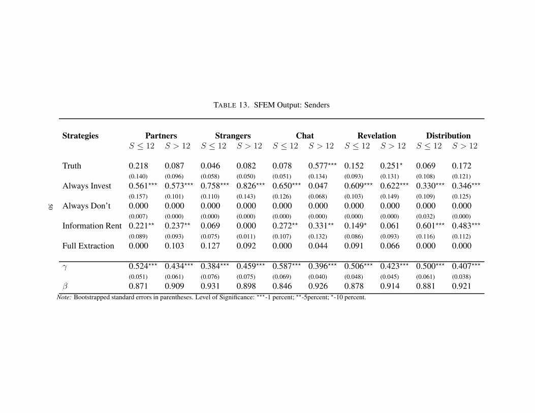
TABLE 13. SFEM Output: Senders

Strategies Partners Strangers Chat Revelation Distribution

S ≤ 12 S > 12 S ≤ 12 S > 12 S ≤ 12 S > 12 S ≤ 12 S > 12 S ≤ 12 S > 12

Truth 0.218 0.087 0.046 0.082 0.078 0.577⋆⋆⋆ 0.152 0.251⋆ 0.069 0.172(0.140) (0.096) (0.058) (0.050) (0.051) (0.134) (0.093) (0.131) (0.108) (0.121)

Always Invest 0.561⋆⋆⋆ 0.573⋆⋆⋆ 0.758⋆⋆⋆ 0.826⋆⋆⋆ 0.650⋆⋆⋆ 0.047 0.609⋆⋆⋆ 0.622⋆⋆⋆ 0.330⋆⋆⋆ 0.346⋆⋆⋆

(0.157) (0.101) (0.110) (0.143) (0.126) (0.068) (0.103) (0.149) (0.109) (0.125)

Always Don’t 0.000 0.000 0.000 0.000 0.000 0.000 0.000 0.000 0.000 0.000(0.007) (0.000) (0.000) (0.000) (0.000) (0.000) (0.000) (0.000) (0.032) (0.000)

Information Rent 0.221⋆⋆ 0.237⋆⋆ 0.069 0.000 0.272⋆⋆ 0.331⋆⋆ 0.149⋆ 0.061 0.601⋆⋆⋆ 0.483⋆⋆⋆

(0.089) (0.093) (0.075) (0.011) (0.107) (0.132) (0.086) (0.093) (0.116) (0.112)

Full Extraction 0.000 0.103 0.127 0.092 0.000 0.044 0.091 0.066 0.000 0.000

γ 0.524⋆⋆⋆ 0.434⋆⋆⋆ 0.384⋆⋆⋆ 0.459⋆⋆⋆ 0.587⋆⋆⋆ 0.396⋆⋆⋆ 0.506⋆⋆⋆ 0.423⋆⋆⋆ 0.500⋆⋆⋆ 0.407⋆⋆⋆

(0.051) (0.061) (0.076) (0.075) (0.069) (0.040) (0.048) (0.045) (0.061) (0.038)

β 0.871 0.909 0.931 0.898 0.846 0.926 0.878 0.914 0.881 0.921Note: Bootstrapped standard errors in parentheses. Level of Significance: ⋆⋆⋆-1 percent; ⋆⋆-5percent; ⋆-10 percent.

50

TABLE 14. SFEM Output: Receivers

Strategies Partners Strangers Chat Revelation Distribution

S ≤ 12 S > 12 S ≤ 12 S > 12 S ≤ 12 S > 12 S ≤ 12 S > 12 S ≤ 12 S > 12

Follow 0.189 0.081 0.217⋆⋆ 0.107 0.174⋆ 0.066 0.024 0.068 0.044 0.072(0.122) (0.054) (0.085) (0.094) (0.094) (0.096) (0.076) (0.063) (0.066) (0.071)

Always Partial 0.217⋆ 0.216⋆ 0.210 0.378⋆⋆⋆ 0.136 0.000 0.167 0.133 0.000 0.204⋆⋆

(0.113) (0.110) (0.137) (0.143) (0.093) (0.048) (0.115) (0.109) (0.062) (0.099)

Always Full 0.000 0.043 0.000 0.000 0.000 0.000 0.035 0.000 0.000 0.000(0.005) (0.056) (0.022) (0.007) (0.002) (0.011) (0.049) (0.006) (0.010) (0.001)

Always None 0.000 0.000 0.000 0.000 0.041 0.000 0.087 0.087 0.000 0.000(0.001) (0.040) (0.006) (0.005) (0.028) (0.000) (0.064) (0.068) (0.008) (0.004)

Partial/None 0.310⋆⋆ 0.446⋆⋆⋆ 0.460⋆⋆⋆ 0.409⋆⋆⋆ 0.370⋆⋆⋆ 0.042 0.315⋆ 0.351⋆⋆ 0.296⋆⋆ 0.302⋆

(0.125) (0.121) (0.117) (0.152) (0.106) (0.061) (0.184) (0.163) (0.134) (0.174)

Information Rent 0.000 0.077 0.114 0.056 0.075 0.893⋆⋆⋆ 0.134 0.173⋆⋆ 0.568⋆⋆⋆ 0.353⋆⋆

(0.043) (0.057) (0.081) (0.054) (0.062) (0.103) (0.126) (0.081) (0.163) (0.156)

Full Extraction 0.284 0.137 0.000 0.049 0.204 0.000 0.237 0.188 0.092 0.070

γ 0.655⋆⋆⋆ 0.544⋆⋆⋆ 0.605⋆⋆⋆ 0.524⋆⋆⋆ 0.647⋆⋆⋆ 0.482⋆⋆⋆ 0.876⋆⋆⋆ 0.590⋆⋆⋆ 0.591⋆⋆⋆ 0.519⋆⋆⋆

(0.100) (0.106) (0.102) (0.099) (0.119) (0.073) (0.194) (0.079) (0.115) (0.082)

β 0.697 0.759 0.723 0.771 0.701 0.799 0.610 0.732 0.731 0.775Note: Bootstrapped standard errors in parentheses. Level of Significance: ⋆⋆⋆-1 percent; ⋆⋆-5percent; ⋆-10 percent.

51