Information to Examinees Sitting for the Fundamentals of Surveying Examination

The Fundamentals of Surveying (FS) examination is a closed-book examination. Therefore, no reference material is allowed in the examination site. The formulas and information here are provided in both the morning and the afternoon examination booklets. This information is not intended to be an all-inclusive compilation of formulas required for the FS examination. Basic theories, conversions, formulas, and definitions that examinees are expected to know have not been included. As required, special material not included here will be provided in the question statement itself to assist the examinee in solving the question. In no event shall NCEES be liable for not providing reference material to support all the questions in the FS examination. NCEES reserves the right to revise and update the information contained here as it deems appropriate without informing interested parties. Each NCEES FS examination will be administered using the latest version of this information.

1

CONVERSIONS AND OTHER USEFUL RELATIONSHIPS

* 1 U.S. survey foot = 12 m39.37

* 1 international foot = 0.3048 m

* 1 in. = 25.4 mm (international)

1 mile = 1.60935 km

* 1 acre = 43,560 ft2 = 10 square chains

* 1 ha = 10,000 m2 = 2.47104 acres

* 1 rad = 180π

1 kg = 2.2046 lb

1 L = 0.2624 gal

1 ft3 = 7.481 gal

1 gal of water weighs 8.34 lb

1 ft3 of water weighs 62.4 lb

1 atm = 29.92 in. Hg = 14.696 psi

Gravity acceleration (g) = 9.807 m/s2 = 32.174 ft/sec2

Speed of light in a vacuum (c) = 299,792,458 m/s = 186,282 miles/sec

°C = (°F – 32)/1.8

1 min of latitude (φ) ≅ 1 nautical mile

1 nautical mile = 6,076 ft

Mean radius of the earth ≅ 20,906,000 ft ≅ 6,372,000 m

* Denotes exact value. All others correct to figures shown.

2

3

AC

c

b

a

B

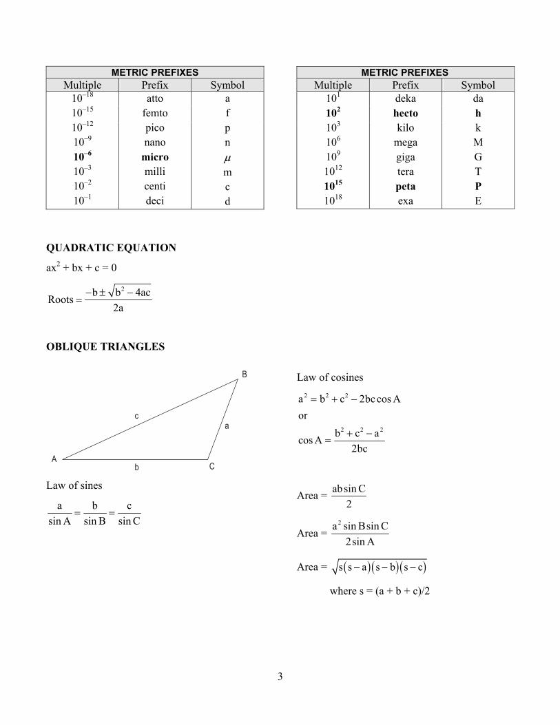
METRIC PREFIXES Multiple Prefix Symbol

10–18

10–15

10–12

10–9

10–6

10–3

10–2

10–1

atto femto pico nano

micro milli centi deci

a f p n µ m c d

METRIC PREFIXES Multiple Prefix Symbol

101

102

103

106

109

1012

1015

1018

deka hecto kilo

mega giga tera peta exa

da h k M G T P E

QUADRATIC EQUATION

ax2 + bx + c = 0

2b b 4acRoots2a

− ± −=

OBLIQUE TRIANGLES

Law of sines

a b csin A sin B sin C

= =

Law of cosines 2 2 2

2 2 2

a b c 2bccos Aor

b c acos A2bc

= + −

+ −=

Area = absin C2

Area = 2a sin Bsin C

2sin A

Area = ( ) ( ) ( )s s a s b s c− − −

where s = (a + b + c)/2

4

SPHERICAL TRIANGLES

A

C

c

b

a

B

Law of sines

sin a sin b sin csin A sin B sin C

= =

Law of cosines

cos a = cos b cos c + sin b sin c cos A 2Area of sphere 4 R= π

34Volume of sphere R3

= π

Spherical excess in sec. = 6 2

bcsin A9.7 10 R−×

where R = mean radius of the earth

angle from the x axis

PROBABILITY AND STATISTICS

( )2 2ix x v

n 1 n 1−

σ = =− −

∑ ∑

where: σ = standard deviation (sometimes

referred to as standard error) Σv2 = sum of the squares of the residuals

(deviation from the mean) n = number of observations x = mean of the observations (individual

measurements xi)

2 2sum 1 2 nσ = σ +σ + +σ… 2

series nσ = σ

mean nσ

σ =

2 2 2 2product b aσ = Α σ +Β σ

2x xy

2xy y

⎡ ⎤σ σΣ = ⎢ ⎥σ σ⎣ ⎦

xy

2x y

2tan 2

σθ=

σ − σ2 where θ = the counter clockwise

Relative weights are inversely proportional to variances, or:

a 2a

1W ∝σ

Weighted mean:

wWM

MW

= ∑∑

where:

Mw = weighted mean ΣWM = sum of individual weights times

their measurements ΣW = sum of the weights

5

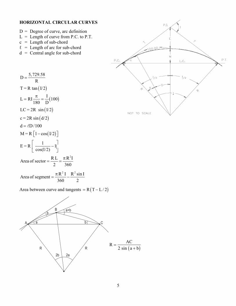
HORIZONTAL CIRCULAR CURVES

D = Degree of curve, arc definition L = Length of curve from P.C. to P.T. c = Length of sub-chord ℓ = Length of arc for sub-chord d = Central angle for sub-chord

5,729.58DR

=

( )T = R tan I/2

( )IL RI 100180 Dπ

= =

( )LC = 2R sin I/2

( )c = 2R sin d/2

d D /100=

( )M = R 1 cos I/2 ⎡ − ⎤⎣ ⎦

1E = R 1 cos(I/2)

⎡ ⎤−⎢ ⎥

⎣ ⎦

2R L R IArea of sector2 360

π= =

2 2R I R sin IArea of segment360 2π

= −

Area between curve and tangents ( )R T L / 2= −

A C

B

R R

2a2b

ba

a+bb

( )ACR

2 sin a b=

+

6

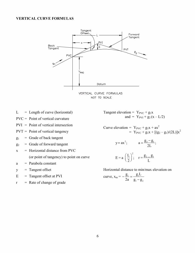
VERTICAL CURVE FORMULAS L = Length of curve (horizontal)

PVC = Point of vertical curvature

PVI = Point of vertical intersection

PVT = Point of vertical tangency

g1 = Grade of back tangent

g2 = Grade of forward tangent

x = Horizontal distance from PVC

(or point of tangency) to point on curve

a = Parabola constant

y = Tangent offset

E = Tangent offset at PVI

r = Rate of change of grade

Tangent elevation = YPVC + g1x and = YPVI + g2 (x – L/2) Curve elevation = YPVC + g1x + ax2 = YPVC + g1x + [(g2 – g1)/(2L)]x2

2y ax ;= 2 1g ga ;2L−

=

2LE = a ;2

⎛ ⎞⎜ ⎟⎝ ⎠

2 1 _ g gr =

L

Horizontal distance to min/max elevation on

curve, xm = 1 1

1 2

g g L2a g g

− =−

7

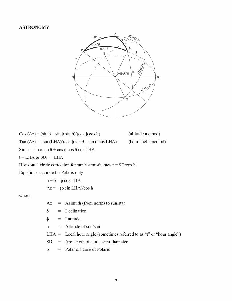
ASTRONOMY

EARTH

φ

h

P

N S

E

W

S

δ

90°− φZ

90°− h

90°− δLHA(t)

HORIZON

EQ

UAT

OR

MERIDIAN

o

Cos (Az) = (sin δ – sin φ sin h)/(cos φ cos h) (altitude method)

Tan (Az) = –sin (LHA)/(cos φ tan δ – sin φ cos LHA) (hour angle method)

Sin h = sin φ sin δ + cos φ cos δ cos LHA

t = LHA or 360° – LHA

Horizontal circle correction for sun’s semi-diameter = SD/cos h

Equations accurate for Polaris only:

h = φ + p cos LHA

Az = – (p sin LHA)/cos h

where:

Az = Azimuth (from north) to sun/star

δ = Declination

φ = Latitude

h = Altitude of sun/star

LHA = Local hour angle (sometimes referred to as “t” or “hour angle”)

SD = Arc length of sun’s semi-diameter

p = Polar distance of Polaris

8

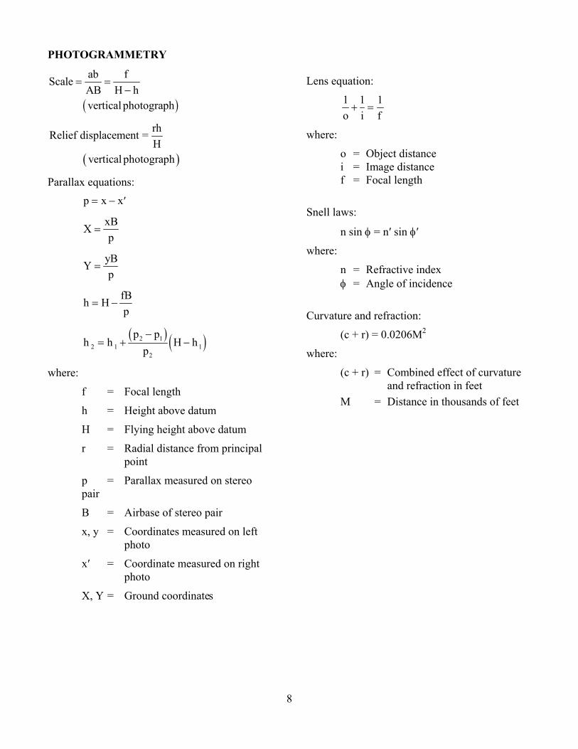
PHOTOGRAMMETRY

( )

ab fScaleAB H hvertical photograph

= =−

( )

rhRelief displacement =H

vertical photograph

Parallax equations: p x x= − ′

xBXp

=

yBYp

=

fBh Hp

= −

( ) ( )2 12 1 1

2

p ph h H h

p−

= + −

where:

f = Focal length

h = Height above datum

H = Flying height above datum

r = Radial distance from principal point

p = Parallax measured on stereo pair

B = Airbase of stereo pair

x, y = Coordinates measured on left photo

x′ = Coordinate measured on right photo

X, Y = Ground coordinates

Lens equation:

1 1 1o i f+ =

where:

o = Object distance i = Image distance f = Focal length

Snell laws:

n sin φ = n′ sin φ′

where:

n = Refractive index φ = Angle of incidence

Curvature and refraction:

(c + r) = 0.0206M2

where:

(c + r) = Combined effect of curvature and refraction in feet M = Distance in thousands of feet

9

GEODESY

Ellipsoid

b

a

N

S

a = semi-major axis b = semi-minor axis

( )

a bFlattening, fa

usually published as1/ f

−=

2 22

2

a bEccentricity, ea−

=

( )( )

2

3 22

a 1 eRadius in meridian, M

1 e sin

−=

− φ

( )1 22 2

aRadius in prime vertical, N1 e sin

=− φ

( )1 22 2

rad

Angular convergence of meridians

d tan 1 e sina

φ − φθ =

( )1 22 2

Linear convergence of meridians

d tan 1 e sina

− φ=

( )m d

D2λ +

=

where: φ = Latitude d = Distance along parallel at latitude φ ℓ = Length along meridians separated by d

Ellipsoid definitions:

GRS80: a = 6,378,137.0 m 1/f = 298.25722101

Clark 1866: a = 6,378,206.4 m 1/f = 294.97869821 Orthometric correction: Correction = −0.005288 sin2φh∆φarc1′ where: φ = latitude at starting point h = datum elevation in meters or feet at starting point ∆φ = change in latitude in minutes between the two points (+ in the direction of increasing latitude or towards the pole)

STATE PLANE COORDINATES

Scale factor = Grid distance/geodetic (ellipsoidal) distance Elevation factor = R/(R + H +N) where:

R = Ellipsoid radius H = Orthometric height N = Geoid height

For precision less than 1/200,000: R = 20,906,000 ft H = Elevation above sea level N = 0

ELECTRONIC DISTANCE MEASUREMENT

V = c/n λ = V/f where:

V = Velocity of light through the atmosphere (m/s) c = Velocity of light in a vacuum n = Index of refraction λ = Wave length (m) f = Modulated frequency in hertz (cycles/sec)

D = Distance measured

10

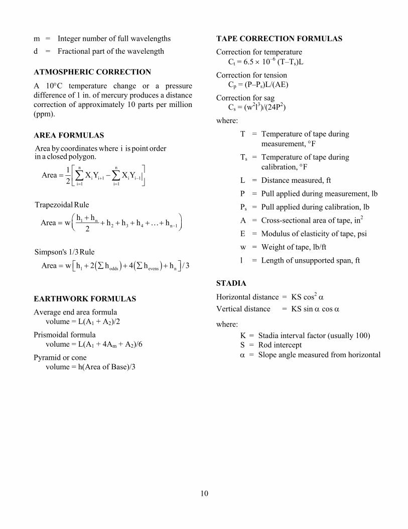
m = Integer number of full wavelengths d = Fractional part of the wavelength

ATMOSPHERIC CORRECTION

A 10°C temperature change or a pressure difference of 1 in. of mercury produces a distance correction of approximately 10 parts per million (ppm).

AREA FORMULAS

n n

i i 1 i i 1i 1 i 1

Area by coordinates where i is point orderin a closed polygon.

1Area X Y X Y2 + −

= =

⎡ ⎤= −⎢ ⎥

⎣ ⎦∑ ∑

1 n2 3 4 n 1

Trapezoidal Ruleh hArea w h h h h

2 −

+⎛= + + + + +⎜⎝ ⎠… ⎞

⎟

⎤

( ) ( )1 odds evens n

Simpson's 1/3Rule

Area w h 2 h 4 h h / 3⎡= + ∑ + ∑ +⎣ ⎦

EARTHWORK FORMULAS

Average end area formula volume = L(A1 + A2)/2

Prismoidal formula volume = L(A1 + 4Am + A2)/6

Pyramid or cone volume = h(Area of Base)/3

TAPE CORRECTION FORMULAS

Correction for temperature Ct = 6.5 × 10–6 (T–Ts)L

Correction for tension Cp = (P–Ps)L/(AE)

Correction for sag Cs = (w2l3)/(24P2)

where:

T = Temperature of tape during measurement, °F

Ts = Temperature of tape during calibration, °F

L = Distance measured, ft

P = Pull applied during measurement, lb

Ps = Pull applied during calibration, lb

A = Cross-sectional area of tape, in2

E = Modulus of elasticity of tape, psi

w = Weight of tape, lb/ft

l = Length of unsupported span, ft

STADIA

Horizontal distance = KS cos2 α Vertical distance = KS sin α cos α

where: K = Stadia interval factor (usually 100) S = Rod intercept α = Slope angle measured from horizontal

11

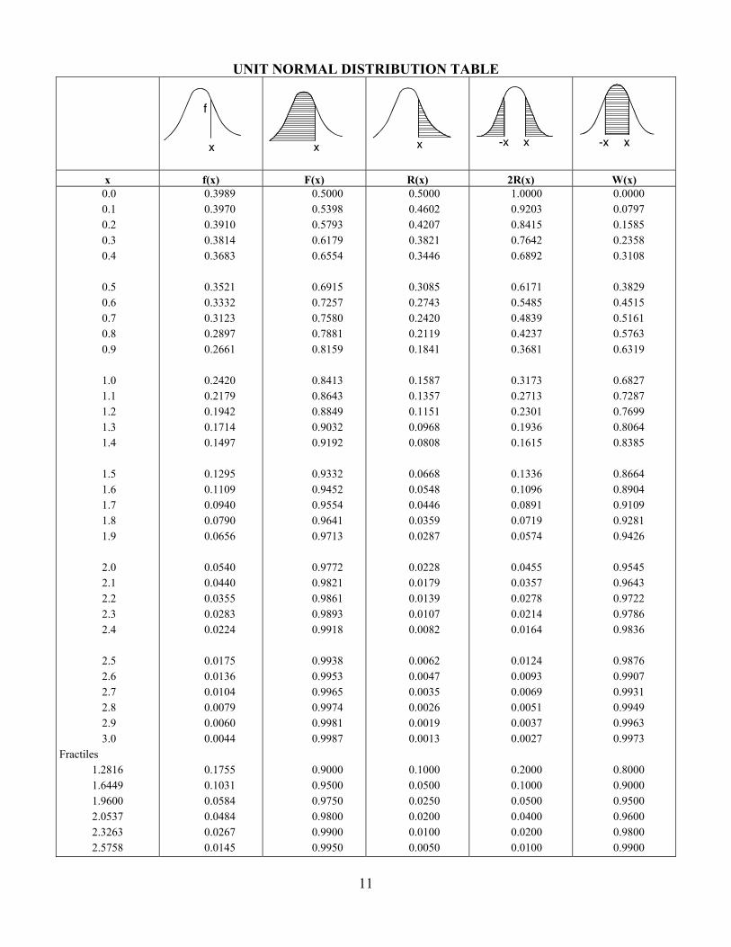
UNIT NORMAL DISTRIBUTION TABLE

x f(x) F(x) R(x) 2R(x) W(x) 0.0 0.1 0.2 0.3 0.4 0.5 0.6 0.7 0.8 0.9 1.0 1.1 1.2 1.3 1.4 1.5 1.6 1.7 1.8 1.9 2.0 2.1 2.2 2.3 2.4 2.5 2.6 2.7 2.8 2.9 3.0 Fractiles 1.2816 1.6449 1.9600 2.0537 2.3263 2.5758

0.3989 0.3970 0.3910 0.3814 0.3683 0.3521 0.3332 0.3123 0.2897 0.2661 0.2420 0.2179 0.1942 0.1714 0.1497 0.1295 0.1109 0.0940 0.0790 0.0656 0.0540 0.0440 0.0355 0.0283 0.0224 0.0175 0.0136 0.0104 0.0079 0.0060 0.0044 0.1755 0.1031 0.0584 0.0484 0.0267 0.0145

0.5000 0.5398 0.5793 0.6179 0.6554 0.6915 0.7257 0.7580 0.7881 0.8159 0.8413 0.8643 0.8849 0.9032 0.9192 0.9332 0.9452 0.9554 0.9641 0.9713 0.9772 0.9821 0.9861 0.9893 0.9918 0.9938 0.9953 0.9965 0.9974 0.9981 0.9987 0.9000 0.9500 0.9750 0.9800 0.9900 0.9950

0.5000 0.4602 0.4207 0.3821 0.3446 0.3085 0.2743 0.2420 0.2119 0.1841 0.1587 0.1357 0.1151 0.0968 0.0808 0.0668 0.0548 0.0446 0.0359 0.0287 0.0228 0.0179 0.0139 0.0107 0.0082 0.0062 0.0047 0.0035 0.0026 0.0019 0.0013 0.1000 0.0500 0.0250 0.0200 0.0100 0.0050

1.0000 0.9203 0.8415 0.7642 0.6892 0.6171 0.5485 0.4839 0.4237 0.3681 0.3173 0.2713 0.2301 0.1936 0.1615 0.1336 0.1096 0.0891 0.0719 0.0574 0.0455 0.0357 0.0278 0.0214 0.0164 0.0124 0.0093 0.0069 0.0051 0.0037 0.0027 0.2000 0.1000 0.0500 0.0400 0.0200 0.0100

0.0000 0.0797 0.1585 0.2358 0.3108 0.3829 0.4515 0.5161 0.5763 0.6319 0.6827 0.7287 0.7699 0.8064 0.8385 0.8664 0.8904 0.9109 0.9281 0.9426 0.9545 0.9643 0.9722 0.9786 0.9836 0.9876 0.9907 0.9931 0.9949 0.9963 0.9973 0.8000 0.9000 0.9500 0.9600 0.9800

0.9900

12

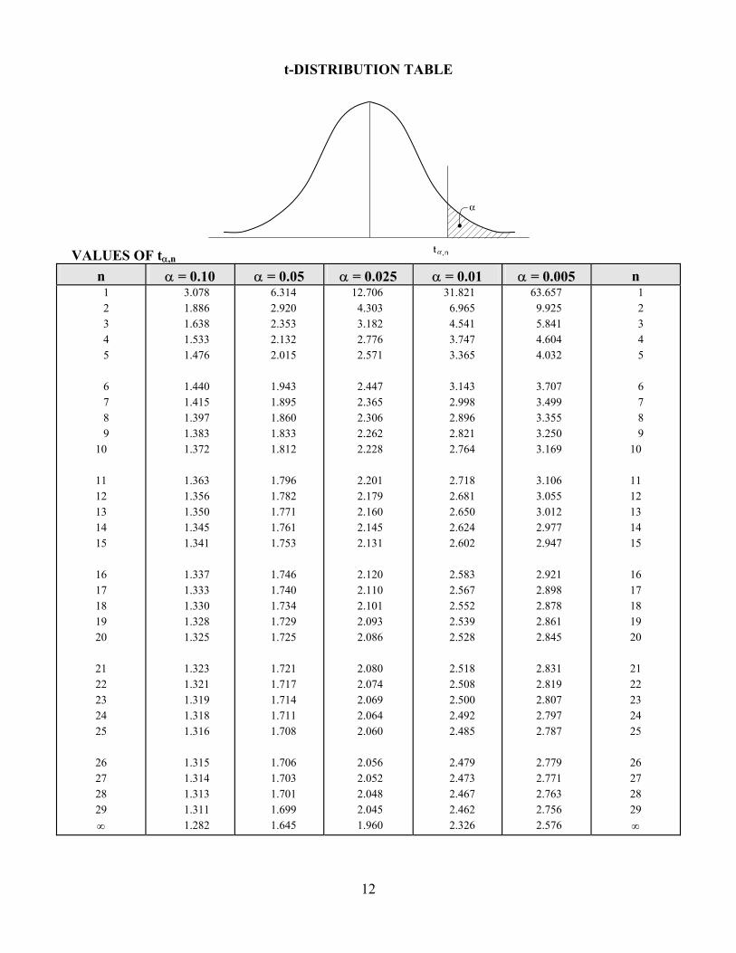
t-DISTRIBUTION TABLE VALUES OF tα,n

n α = 0.10 α = 0.05 α = 0.025 α = 0.01 α = 0.005 n 1 2 3 4 5 6 7 8 9 10 11 12 13 14 15 16 17 18 19 20 21 22 23 24 25 26 27 28 29 ∞

3.078 1.886 1.638 1.533 1.476 1.440 1.415 1.397 1.383 1.372 1.363 1.356 1.350 1.345 1.341 1.337 1.333 1.330 1.328 1.325 1.323 1.321 1.319 1.318 1.316 1.315 1.314 1.313 1.311 1.282

6.314 2.920 2.353 2.132 2.015 1.943 1.895 1.860 1.833 1.812 1.796 1.782 1.771 1.761 1.753 1.746 1.740 1.734 1.729 1.725 1.721 1.717 1.714 1.711 1.708 1.706 1.703 1.701 1.699 1.645

12.706 4.303 3.182 2.776 2.571 2.447 2.365 2.306 2.262 2.228 2.201 2.179 2.160 2.145 2.131 2.120 2.110 2.101 2.093 2.086 2.080 2.074 2.069 2.064 2.060 2.056 2.052 2.048 2.045 1.960

31.821 6.965 4.541 3.747 3.365 3.143 2.998 2.896 2.821 2.764 2.718 2.681 2.650 2.624 2.602 2.583 2.567 2.552 2.539 2.528 2.518 2.508 2.500 2.492 2.485 2.479 2.473 2.467 2.462 2.326

63.657 9.925 5.841 4.604 4.032 3.707 3.499 3.355 3.250 3.169 3.106 3.055 3.012 2.977 2.947 2.921 2.898 2.878 2.861 2.845 2.831 2.819 2.807 2.797 2.787 2.779 2.771 2.763 2.756 2.576

1 2 3 4 5 6 7 8 9 10 11 12 13 14 15 16 17 18 19 20 21 22 23 24 25 26 27 28 29 ∞

α

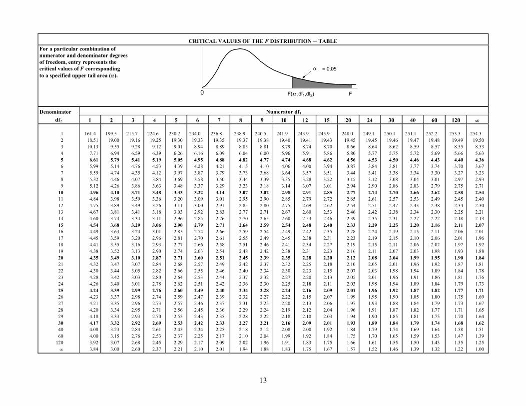
CRITICAL VALUES OF THE F DISTRIBUTION – TABLE For a particular combination of numerator and denominator degrees of freedom, entry represents the critical values of F corresponding to a specified upper tail area (α).

Numerator df1Denominator df2 1 2 3 4 5 6 7 8 9 10 12 15 20 24 30 40 60 120 ∞

1 2 3 4 5 6 7 8 9 10 11 12 13 14 15 16 17 18 19 20 21 22 23 24 25 26 27 28 29 30 40 60 120 ∞

161.4 18.51 10.13 7.71 6.61

5.99 5.59 5.32 5.12 4.96 4.84 4.75 4.67 4.60 4.54 4.49 4.45 4.41 4.38 4.35 4.32 4.30 4.28 4.26 4.24 4.23 4.21 4.20 4.18

4.17 4.08 3.23 4.00 3.15 3.92 3.07 3.84 3.00

199.5 19.00

9.55 6.94 5.79 5.14 4.74 4.46 4.26 4.10 3.98 3.89 3.81 3.74 3.68 3.63 3.59 3.55 3.52 3.49 3.47 3.44 3.42 3.40 3.39 3.37 3.35 3.34 3.33

3.32

215.7

19.16 9.28 6.59 5.41 4.76 4.35 4.07 3.86 3.71 3.59 3.49 3.41 3.34 3.29 3.24 3.20 3.16 3.13 3.10 3.07 3.05 3.03 3.01 2.99 2.98 2.96 2.95 2.93 2.92 2.84 2.76 2.68 2.60

224.6 19.25 9.12 6.39 5.19 4.53 4.12 3.84 3.63 3.48 3.36 3.26 3.18 3.11 3.06 3.01 2.96 2.93 2.90 2.87 2.84 2.82 2.80 2.78 2.76 2.74 2.73 2.71 2.70 2.69 2.61 2.53 2.45 2.37

230.2 19.30 9.01 6.26 5.05 4.39 3.97 3.69 3.48 3.33 3.20 3.11 3.03 2.96 2.90 2.85 2.81 2.77 2.74 2.71 2.68 2.66 2.64 2.62 2.60 2.59 2.57 2.56 2.55 2.53 2.45 2.37 2.29 2.21

234.0 19.33 8.94 6.16 4.95 4.28 3.87 3.58 3.37 3.22 3.09 3.00 2.92 2.85 2.79 2.74 2.70 2.66 2.63 2.60 2.57 2.55 2.53 2.51 2.49 2.47 2.46 2.45 2.43 2.42 2.34 2.25 2.17 2.10

236.8 19.35 8.89 6.09 4.88 4.21 3.79 3.50 3.29 3.14 3.01 2.91 2.83 2.76 2.71 2.66 2.61 2.58 2.54 2.51 2.49 2.46 2.44 2.42 2.40 2.39 2.37 2.36 2.35 2.33 2.25 2.17 2.09 2.01

238.9 19.37

8.85 6.04 4.82 4.15 3.73 3.44 3.23 3.07 2.95 2.85 2.77 2.70 2.64 2.59 2.55 2.51 2.48 2.45 2.42 2.40 2.37 2.36 2.34 2.32 2.31 2.29 2.28

2.27 2.18 2.10 2.02 1.94

240.5 19.38 8.81 6.00 4.77 4.10 3.68 3.39 3.18 3.02 2.90 2.80 2.71 2.65 2.59 2.54 2.49 2.46 2.42 2.39 2.37 2.34 2.32 2.30 2.28 2.27 2.25 2.24 2.22 2.21 2.12 2.04 1.96 1.88

241.9 19.40 8.79 5.96 4.74 4.06 3.64 3.35 3.14 2.98 2.85 2.75 2.67 2.60 2.54 2.49 2.45 2.41 2.38 2.35 2.32 2.30 2.27 2.25 2.24 2.22 2.20 2.19 2.18 2.16 2.08 1.99 1.91 1.83

243.9 19.41 8.74 5.91 4.68 4.00 3.57 3.28 3.07 2.91 2.79 2.69 2.60 2.53 2.48 2.42 2.38 2.34 2.31 2.28 2.25 2.23 2.20 2.18 2.16 2.15 2.13 2.12 2.10 2.09 2.00 1.92 1.83 1.75

245.9 19.43 8.70 5.86 4.62 3.94 3.51 3.22 3.01 2.85 2.72 2.62 2.53 2.46 2.40 2.35 2.31 2.27 2.23 2.20 2.18 2.15 2.13 2.11 2.09 2.07 2.06 2.04 2.03 2.01 1.92 1.84 1.75 1.67

248.0 19.45 8.66 5.80 4.56 3.87 3.44 3.15 2.94 2.77 2.65 2.54 2.46 2.39 2.33 2.28 2.23 2.19 2.16 2.12 2.10 2.07 2.05 2.03 2.01 1.99 1.97 1.96 1.94 1.93 1.84 1.75 1.66 1.57

249.1 19.45 8.64 5.77 4.53 3.84 3.41 3.12 2.90 2.74 2.61 2.51 2.42 2.35 2.29 2.24 2.19 2.15 2.11 2.08 2.05 2.03 2.01 1.98 1.96 1.95 1.93 1.91 1.90 1.89 1.79 1.70 1.61 1.52

250.1 19.46 8.62 5.75 4.50 3.81 3.38 3.08 2.86 2.70 2.57 2.47 2.38 2.31 2.25 2.19 2.15 2.11 2.07 2.04 2.01 1.98 1.96 1.94 1.92 1.90 1.88 1.87 1.85 1.84 1.74 1.65 1.55 1.46

251.1 19.47 8.59 5.72 4.46 3.77 3.34 3.04 2.83 2.66 2.53 2.43 2.34 2.27 2.20 2.15 2.10 2.06 2.03 1.99 1.96 1.94 1.91 1.89 1.87 1.85 1.84 1.82 1.81 1.79 1.69 1.59 1.50 1.39

252.2 19.48 8.57 5.69 4.43 3.74 3.30 3.01 2.79 2.62 2.49 2.38 2.30 2.22 2.16 2.11 2.06 2.02 1.98 1.95 1.92 1.89 1.86 1.84 1.82 1.80 1.79 1.77 1.75 1.74 1.64 1.53 1.43 1.32

253.3 19.49 8.55 5.66 4.40 3.70 3.27 2.97 2.75 2.58 2.45 2.34 2.25 2.18 2.11 2.06 2.01 1.97 1.93 1.90 1.87 1.84 1.81 1.79 1.77 1.75 1.73 1.71 1.70 1.68 1.58 1.47 1.35 1.22

254.3 19.50

8.53 5.63 4.36 3.67 3.23 2.93 2.71 2.54 2.40 2.30 2.21 2.13 2.07 2.01 1.96 1.92 1.88 1.84 1.81 1.78 1.76 1.73 1.71 1.69 1.67 1.65 1.64

1.62 1.51 1.39 1.25 1.00

13

14

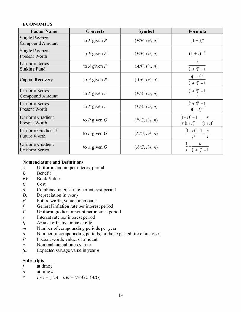
ECONOMICS Factor Name Converts Symbol Formula

Single Payment Compound Amount to F given P (F/P, i%, n) (1 + i)n

Single Payment Present Worth to P given F (P/F, i%, n) (1 + i) –n

Uniform Series Sinking Fund to A given F (A/F, i%, n) ( ) 11 −+ ni

i

Capital Recovery to A given P (A/P, i%, n) ( )

( ) 111

−+

+n

n

iii

Uniform Series Compound Amount to F given A (F/A, i%, n) ( )

ii n 11 −+

Uniform Series Present Worth to P given A (P/A, i%, n)

( )( )n

n

iii+

−+

111

Uniform Gradient Present Worth to P given G (P/G, i%, n)

( )( ) ( )nn

n

iin

iii

+−

+

−+

1111

2

Uniform Gradient † Future Worth to F given G (F/G, i%, n) ( )

in

ii n

−−+

211

Uniform Gradient Uniform Series to A given G (A/G, i%, n) ( ) 11

1−+

− nin

i

Nomenclature and Definitions A Uniform amount per interest period B Benefit BV Book Value C Cost d Combined interest rate per interest period Dj Depreciation in year j F Future worth, value, or amount f General inflation rate per interest period G Uniform gradient amount per interest period i Interest rate per interest period ie Annual effective interest rate m Number of compounding periods per year n Number of compounding periods; or the expected life of an asset P Present worth, value, or amount r Nominal annual interest rate Sn Expected salvage value in year n

Subscripts j at time j n at time n † F/G = (F/A – n)/i = (F/A) × (A/G)

Nonannual Compounding

11 −⎟⎠⎞

⎜⎝⎛ +=

m

e mri

Book Value BV = Initial cost – Σ Dj

Depreciation Straight line

nSCD n

j−

=

Accelerated Cost Recovery System (ACRS)

Dj = (factor from table below) C

MODIFIED ACRS FACTORS Recovery Period (Years)

3 5 7 10 Year Recovery Rate (%)

1 2 3 4 5 6 7 8 9 10 11

33.3 44.5 14.8 7.4

20.0 32.0 19.2 11.5 11.5 5.8

14.3 24.5 17.5 12.5

8.9 8.9 8.9 4.5

10.0 18.0 14.4 11.5 9.2 7.4 6.6 6.6 6.5 6.5 3.3

Capitalized Costs Capitalized costs are present worth values using an assumed perpetual period of time. Capitalized costs = P =

iA

15