inflow/outflow boundary conditions with application … · 10.01.2011 · inflow/outflow boundary...

October 2011

NASA/TM–2011-217181

Inflow/Outflow Boundary Conditions with Application to FUN3D

Jan-Reneé Carlson Langley Research Center, Hampton, Virginia

NASA STI Program . . . in Profile

Since its founding, NASA has been dedicated to the advancement of aeronautics and space science. The NASA scientific and technical information (STI) program plays a key part in helping NASA maintain this important role.

The NASA STI program operates under the auspices of the Agency Chief Information Officer. It collects, organizes, provides for archiving, and disseminates NASA’s STI. The NASA STI program provides access to the NASA Aeronautics and Space Database and its public interface, the NASA Technical Report Server, thus providing one of the largest collections of aeronautical and space science STI in the world. Results are published in both non-NASA channels and by NASA in the NASA STI Report Series, which includes the following report types:

� TECHNICAL PUBLICATION. Reports of completed research or a major significant phase of research that present the results of NASA programs and include extensive data or theoretical analysis. Includes compilations of significant scientific and technical data and information deemed to be of continuing reference value. NASA counterpart of peer-reviewed formal professional papers, but having less stringent limitations on manuscript length and extent of graphic presentations.

� TECHNICAL MEMORANDUM. Scientific and technical findings that are preliminary or of specialized interest, e.g., quick release reports, working papers, and bibliographies that contain minimal annotation. Does not contain extensive analysis.

� CONTRACTOR REPORT. Scientific and technical findings by NASA-sponsored contractors and grantees.

� CONFERENCE PUBLICATION. Collected papers from scientific and technical conferences, symposia, seminars, or other meetings sponsored or co-sponsored by NASA.

� SPECIAL PUBLICATION. Scientific, technical, or historical information from NASA programs, projects, and missions, often concerned with subjects having substantial public interest.

� TECHNICAL TRANSLATION. English-language translations of foreign scientific and technical material pertinent to NASA’s mission.

Specialized services also include creating custom thesauri, building customized databases, and organizing and publishing research results.

For more information about the NASA STI program, see the following:

� Access the NASA STI program home page at http://www.sti.nasa.gov

� E-mail your question via the Internet to [email protected]

� Fax your question to the NASA STI Help Desk at 443-757-5803

� Phone the NASA STI Help Desk at 443-757-5802

� Write to: NASA STI Help Desk NASA Center for AeroSpace Information 7115 Standard Drive Hanover, MD 21076-1320

National Aeronautics and Space Administration

Langley Research Center Hampton, Virginia 23681-2199

October 2011

NASA/TM–2011-217181


Jan-Reneé Carlson Langley Research Center, Hampton, Virginia

Available from:

NASA Center for AeroSpace Information 7115 Standard Drive

Hanover, MD 21076-1320 443-757-5802

The use of trademarks or names of manufacturers in this report is for accurate reporting and does not constitute an official endorsement, either expressed or implied, of such products or manufacturers by the National Aeronautics and Space Administration.

Abstract

Several boundary conditions that allow subsonic and supersonic flow into and out of thecomputational domain are discussed. These boundary conditions are demonstrated inthe FUN3D computational fluid dynamics (CFD) code which solves the three-dimensionalNavier-Stokes equations on unstructured computational meshes. The boundary conditionsare enforced through determination of the flux contribution at the boundary to the solutionresidual. The boundary conditions are implemented in an implicit form where the Jacobiancontribution of the boundary condition is included and is exact. All of the flows are gov-erned by the calorically perfect gas thermodynamic equations. Three problems are used toassess these boundary conditions. Solution residual convergence to machine zero precisionoccurred for all cases. The converged solution boundary state is compared with the re-quested boundary state for several levels of mesh densities. The boundary values convergedto the requested boundary condition with approximately second-order accuracy for all ofthe cases.

1 Introduction

The solution of a partial differential equation or a system of partial differential equationsrequires a statement of the dependent variables along the boundaries of the solution

space. When physically relevant solutions of the equations are sought, the imposition of theboundary conditions should solve the correct numerical problem without adversely affectingsolution stability.

The choice between an explicit or implicit implementation of the boundary conditionsin the solution algorithm is dependent on the numerical method that is used for solving thegoverning equations. Explicit treatments of boundary conditions has occupied much of theliterature. The compilation of papers in the proceedings Numerical Boundary ConditionProcedures [1] contains extensive discussions of the state-of-the-art theories at the time ofprinting. In particular, Moretti [2], Blottner [3], Pulliam [4], and Thompkins and Bush [5]discuss inflow and outflow boundary conditions for both Navier-Stokes and Euler equations.

Much of that work centered around developing a system of equations, often in terms ofcharacteristic variables, to describe the desired physical state in a consistent form at theboundary. Information is communicated through the boundary interface via wave propaga-tion and convection. The flow of information across the boundary determines the physicalconditions to impose. Thus, the boundary conditions must be formulated to keep the so-lution realizable at the boundary. The interior solution will be consistent with the speci-fied physical state at all of the boundaries once an iteratively converged solution has beenachieved.

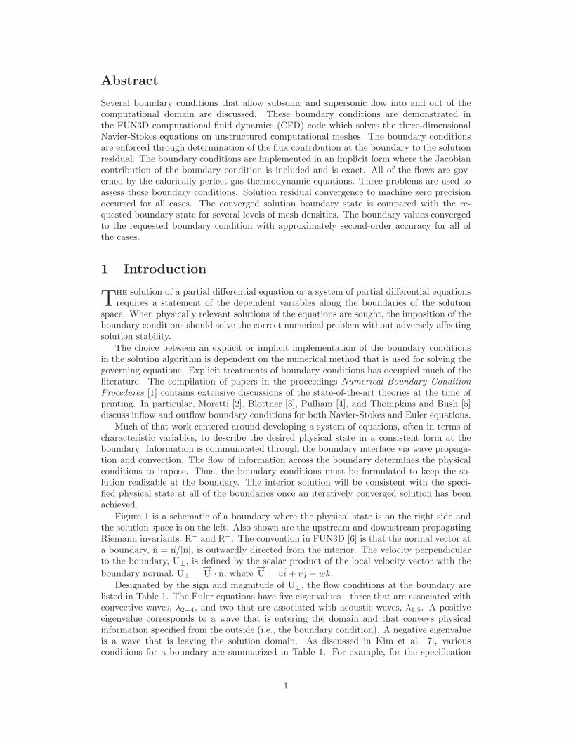
Figure 1 is a schematic of a boundary where the physical state is on the right side andthe solution space is on the left. Also shown are the upstream and downstream propagatingRiemann invariants, R− and R+. The convention in FUN3D [6] is that the normal vector ata boundary, n = �n/|�n|, is outwardly directed from the interior. The velocity perpendicularto the boundary, U⊥, is defined by the scalar product of the local velocity vector with theboundary normal, U⊥ =

−→U · n, where

−→U = ui + vj + wk.

Designated by the sign and magnitude of U⊥, the flow conditions at the boundary arelisted in Table 1. The Euler equations have five eigenvalues—three that are associated withconvective waves, λ2−4, and two that are associated with acoustic waves, λ1,5. A positiveeigenvalue corresponds to a wave that is entering the domain and that conveys physicalinformation specified from the outside (i.e., the boundary condition). A negative eigenvalueis a wave that is leaving the solution domain. As discussed in Kim et al. [7], variousconditions for a boundary are summarized in Table 1. For example, for the specification

1

Interior state Requestedphysical state

Inside the domain Outside the domain

��

��

��

�� R+ = Ui + 2ciγ−1

R− = Ub − 2cbγ−1

� �n

Figure 1. Characteristics at a boundary.

of a subsonic inflow boundary with the use of primitive variables, density and velocity ordensity and pressure are combinations that can be used to completely define the condition.In practice, many methods are used to enforce a particular condition at a boundary interface.In this work, the boundary conditions are enforced weakly, that is, by calculating andapplying the flux contribution of the boundary condition to the solution residual ratherthan setting the physical value of the boundary condition.

The details of each boundary condition are discussed in a generic framework in section 2;and a discussion of the discrete, computational method used for evaluation of the boundaryconditions in FUN3D follows in section 3. Three test geometries are described in section 4.Computations that demonstrate the use of the boundary conditions are given in section 5.

Table 1. Flow Conditions at a Boundary

Case Condition U⊥ |U⊥| EigenvalueSpecify

λ1 λ2 λ3 λ4 λ5

1 Subsonic inflow <0 <c <0 >0 >0 >0 >0 pt, Tt, α, β*

2 Subsonic outflow >0 <c <0 <0 <0 <0 >0 p3 Supersonic inflow <0 >c >0 >0 >0 >0 >0 All4 Supersonic outflow >0 >c <0 <0 <0 <0 <0 None

*Alternatively ρ and−→U or ρ and p, but not

−→U and p.

2 Boundary Conditions

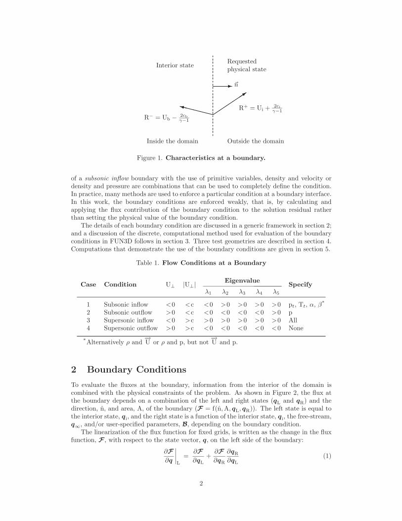
To evaluate the fluxes at the boundary, information from the interior of the domain iscombined with the physical constraints of the problem. As shown in Figure 2, the flux atthe boundary depends on a combination of the left and right states (qL and qR) and thedirection, n, and area, A, of the boundary (F = f(n, A, qL, qR)). The left state is equal tothe interior state, qi, and the right state is a function of the interior state, qi, the free-stream,q∞, and/or user-specified parameters, B, depending on the boundary condition.

The linearization of the flux function for fixed grids, is written as the change in the fluxfunction, F , with respect to the state vector, q, on the left side of the boundary:

∂F∂q

∣∣∣∣L

=∂F∂qL

+∂F∂qR

∂qR

∂qL

(1)

2

Left state Right state

qL = qi qR = f(qi, q∞,B)

FFigure 2. Flux and boundary states.

The first two derivatives, ∂F/∂qL and ∂F/∂qR, are the Jacobians for the numerical fluxfunction used in the spatial differencing. FUN3D provides multiple options for the numericalflux function. The results in this work use Roe’s approximate flux scheme and the Jacobianterms of Roe’s scheme were handcoded term-by-term. The third term, ∂qR/∂qL, is deter-mined exactly by using automatic differentiation via operator overloading of the equationsin the boundary condition functions in Griewank and Corliss [8, 9]. This differentiationtechnique, which is based on the chain rule, permits the partial derivatives of the boundarycondition variables with respect to the interior variables to be calculated and propagatedthrough each of the boundary condition function calls and results in the Jacobian term ofthe boundary conditions.

Depending upon the specific application, the four inflow/outflow conditions listed inTable 1 ( that is, subsonic inflow/outflow and supersonic inflow/outflow ) can be formed indifferent ways. Several methods for determining the boundary state, qR, are discussed insections 2.1 through 2.9. For each boundary condition, the format of the introductory tableis as follows: the type of condition, the specified conditions, variables that are extrapolatedfrom the interior, and variables that are updated as a consequence of applying the boundarycondition. Words expressed with the fixed-width font indicate code variables that occurwithin FUN3D.

Variables with dimensions are denoted by an overhead ˜ symbol. Non-dimensional vari-ables are denoted without any symbol overhead. Freestream values are denoted by thesubscript ∞ . The equations relating the dimensional to the non-dimensional flow-fieldvariables are as follows:

ρ = ρρ∞, u = u c∞, v = v c∞, w = w c∞, p = p ρ∞c2∞ (2)

e = e ρ∞ c2∞, c = c c∞, T = T T∞ = c2 T∞ (3)

ρ∞ = 1, p∞ = 1/γ, c∞ = 1, T∞ = 1 (4)u∞ = M∞ cos α∞ cos β∞, v∞ = −M∞ sin β∞, w∞ = M∞ sin α∞ cos β∞ (5)

The equations in the subsequent sections are written in their non-dimensional form.

2.1 Far-Field Boundary Condition (farfield roe)

Type Specify Extrapolate Update

Outflow M∞, [M∞ ≥ 0], α∞, β∞ None All

The far-field boundary condition specifies the free-stream conditions that are calculatedfrom the user input variables M∞, α∞, and β∞.

ρ∞ = 1, c∞ = 1, p∞ =ρ∞c2

∞γ

,−→U∞ =

⎡⎣ M∞ cos α∞ cos β∞

−M∞ sin β∞M∞ sin α∞ cos β∞

⎤⎦ (6)

3

The right-state vector is:

qR =

⎡⎣ ρ∞−→

U∞p∞

⎤⎦ (7)

2.2 Riemann Invariant Boundary Condition (riemann)


Inflow/outflow M∞ [M∞ ≥ 0] Entropy (outflow) ρ, p

The Riemann invariants correspond to the incoming R− and outgoing R+ characteristicwaves. The invariants determine the locally normal velocity component and the speed ofsound. The entropy, s, and the speed of sound, c, are used to determine the density andpressure on the boundary (see Figure 1.) The incoming Riemann invariant uses the far-fieldconditions, qo =

[ρ∞,

−→U∞, p∞

]T.

R+ = Ui +2ci

γ − 1, R− = Uo − 2co

γ − 1(8)

where

Ui =−→U i · n,

−→U i = [ui, vi, wi]

T, c2

i =γpi

ρi(9)

Uo =−→U o · n,

−→U o = [uo, vo, wo]

T, c2

o =γpo

ρo(10)

Mi =|Ui|ci

(11)

If the flow at the boundary is locally supersonic leaving the domain (Mi ≥ 1), then noincoming characteristic waves exist; thus, R− is set equal to

R− = Ui − 2ci

γ − 1(12)

Similarly, if the flow is supersonic entering the domain, then no outgoing characteristicwaves exist and R+ is set equal to

R+ = Uo +2co

γ − 1(13)

A velocity, Ub, and the speed of sound, cb, at the boundary are the sum and difference ofthe invariants:

Ub =12(R+ + R−)

, cb = 4 (γ − 1)(R+ − R−)

(14)

The velocity that is imposed on the boundary depends on the local direction of flow. Ifthe sign of U⊥ is positive, then the flow is exiting the computational domain and theentropy is extrapolated from the interior and is used to update the density at the boundary.Conversely, a negative U⊥ indicates that the flow is entering the computational domain and

4

the free-stream entropy is used. Summarizing, the velocity and entropy on the boundaryare calculated from the following equations.

−→Ub =

{−→U i + (U − Ui)n, if U > 0 (outflow)−→U o + (U − Uo)n, if U ≤ 0 (inflow)

(15)

sb =

⎧⎨⎩

c2iγργ−1

i, if U⊥ > 0 (outflow)

c2oγργ−1

o, if U⊥ ≤ 0 (inflow)

(16)

The density and pressure on the boundary are then calculated as follows.

ρb =(

c2b

γsb

)1/γ−1

, pb =ρbc2

b

γ(17)

The right-side vector is

qR =

⎡⎣ ρb−→

Ub

pb

⎤⎦ . (18)

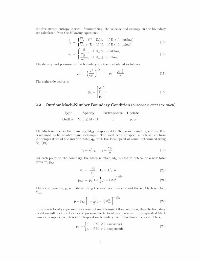
2.3 Outflow Mach-Number Boundary Condition (subsonic outflow mach)


Outflow M [0 ≤ M < 1] T ρ, p

The Mach number at the boundary, Mset, is specified for the entire boundary, and the flowis assumed to be adiabatic and isentropic. The local acoustic speed is determined fromthe temperature of the interior state, qi, with the local speed of sound determined usingEq. (19).

ci =√

Ti, Ti =γpi

ρi(19)

For each point on the boundary, the Mach number, Mi, is used to determine a new totalpressure, pt,b.

Mi =|Ui|ci

, Ui =−→U i · n (20)

pt,b = pi

[1 +

12(γ − 1)M2

i

] γγ−1

(21)

The static pressure, p, is updated using the new total pressure and the set Mach number,Mset

p = pt,b

[1 +

12(γ − 1)M2

set

]− γγ−1

(22)

If the flow is locally supersonic as a result of some transient flow condition, then the boundarycondition will reset the local static pressure to the local total pressure. If the specified Machnumber is supersonic, then an extrapolation boundary condition should be used. Thus,

pb =

{p, if Mi < 1 (subsonic)pt, if Mi > 1 (supersonic)

(23)

5

The right-state state is written as:

qR =

⎡⎣γpb/Ti−→

U i

pb

⎤⎦ (24)

Note: Using this condition is inconsistent if the boundary face adjoins a viscous surface.The Mach number is fixed over the entire boundary and precludes the presence of a velocitygradient that would normally be present on the viscous no-slip surface. A constant pressureboundary condition, such as the subsonic outflow boundary, should be used in this situation.

2.4 Pressure Outflow Boundary Condition (back pressure)


Outflow p/p∞ [p/p∞ > 0]−→U, T ρ

For a subsonic outflow boundary condition, the static pressure ratio, pset/p∞, is specified,while the velocities and temperature are extrapolated. The boundary flow is assumed to beadiabatic and isentropic. The density is updated from the extrapolated temperature andthe requested static pressure. If the flow is supersonic at this boundary, then all quantitiesare extrapolated. The pressure is calculated as

pb =

{pset, if Mi < 1 (subsonic)pi, if Mi ≥ 1 (supersonic)

(25)

and the right-side vector is

qR =

⎡⎣γpb/Ti−→

U i

pb

⎤⎦, Ti =

γpi

ρi(26)

2.5 Subsonic Outflow Boundary Condition (subsonic outflow p0)


Outflow p/p∞ [p/p∞ > 0]−→U, T ρ

The manner in which this boundary specifies the static pressure ratio is the same as thatpresented in section 2.4 but with different implementation details. If any reverse flow (i.e.,flow into the computational domain) occurs, setting the static pressure at the boundaryis numerically ill-posed. This boundary condition will explicitly set the flow to exit thedomain. The flow is also forced to remain subsonic by setting the local static pressure tothe local total pressure if the local Mach number is greater than one. The velocities, Ui, andthe temperature, Ti = γpi/ρi, are extrapolated from the interior solution. The pressure is

pb =

{pset, if Mi < 1 (subsonic)pt, if Mi > 1 (supersonic)

(27)

6

and the velocity is

−→Ub =

{−→U i, if U⊥ > 0 (outflow)|Ui|n, if U⊥ < 0 (inflow)

, U⊥ =−→U i · n (28)

The right-side vector is

qR =

⎡⎣γpb/Ti−→

Ub

pset

⎤⎦ (29)

2.6 Mass Flow Out Boundary Condition (massflux out)


Outflow m [m ≥ 0]−→U, T ρ, p

This boundary condition allows for specification of the mass flow out of the computationaldomain. Adiabatic flow through the boundary is assumed, and the method iterativelymodifies the static pressure for the entire boundary to obtain the requested mass flowcondition. The choice of equations solved for this boundary condition is from the CFD codeVULCAN [10].

The boundary values of momentum thrust Eq.(30), pressure force Eq.(31), and mass flowEq.(32), are calculated by using the following integrals, where the domain of the integrationis the entire boundary face:

Fm =∫

boundary

ρ(−→

U · n)2

dA, (momentum thrust) (30)

Fp =∫

boundary

p dA, (pressure force) (31)

m =∫

boundary

ρ(−→

U · n)

dA, (mass flow) (32)

The static pressure is updated with a form of the continuity equation:

pb =1A

[Fmδm + Fp

], δm =

(1 − mset

m

)(33)

The velocity and the temperature are extrapolated from the interior computational domainso that the right-state vector is:

qR =

⎡⎣γpb/Ti−→

U i

pb

⎤⎦ (34)

2.7 Subsonic Inflow Boundary Condition (subsonic inflow pt)


Inflow pt/p∞, Tt/T∞, n p, R+, Ht ρ,−→U

7

The user can specify the direction of the velocity at the boundary either by the flow angles(αset and βset) relative to the global coordinate axis, or as normal to the boundary, nb.

n =

{cos αset cos βset i − sin βset j + sinαset sin βset k

nb

(35)

The right-side vector, qR, is determined from the outward propagating invariant, R+, anda statement of the total enthalpy, Ht, at an element face on the boundary. The formulationof this boundary condition is the same as that used in [10], which assumes that the flowthrough the boundary is adiabatic and isentropic. Following these assumptions, we write

Hti =pi

ρi

(γ

γ − 1

)+

12

(u2

i + v2i + w2

i

)(36)

R+ = −Ui − 2ci

γ − 1(37)

Because the flow is adiabatic, that is, the total enthalpy is conserved across the boundary,we can state that

Ht =c2b

γ − 1+

12U2

b (38)

Then, by extrapolating R− to the boundary, we obtain

R+ = −Ub − 2cb

γ − 1(39)

By combining Eqs. (39) and (38), we obtain

Ht =c2b

γ − 1+

12

(R+ +

2cb

γ − 1

)2

(40)

Equation (40) is solved for cb, which is the sonic speed at the boundary, by rewriting it asa quadratic equation of the form[

1 +2

(γ − 1)

]c2b + 2R+cb +

γ − 12

(R+2 − 2Ht

)= 0 (41)

The solution has the form

cb± = − b

2a±

√b2 − 4ac

2a(42)

where a, b, and c are the coefficients of the quadratic equation (Eq. 41):

a = 1 +2

(γ − 1), b = 2R+, c =

γ − 12

(R+2 − 2Ht

)(43)

The physically consistent result is the larger of the two roots and is chosen to update thesonic velocity at the boundary:

cb = max(cb+ , cb−) (44)

The updated inflow velocity and the Mach number at the boundary are then computed byusing

U =2cb

γ − 1− R+, Mb =

Ucb

(45)

8

The static pressure and temperature are calculated from the isentropic relations

pb = pt,set

(1 +

γ − 12

M2b

) γγ−1

, Tb = Tt,set

(pb

pt,set

)γ−1γ

(46)

The primitive variables that are determined from the input boundary conditions are placedin the right state qR as

qR =

⎡⎣pb/RTb

Unpb

⎤⎦ (47)

2.8 Mass Flow In Boundary Condition (massflux in)


Inflow m [m ≥ 0], Tt/T∞ ρ p

Mass flow into the computational domain through this boundary condition is updated byadjusting the static temperature, T, at the boundary through a form of the energy equation:

cpT +U

2

2= cpTt,set (48)

The variable, Tt,set, in Eq. (48) is the user-specified total temperature at the boundary,and the flow is assumed to be isentropic and adiabatic through the boundary face. Anexpression for the velocity is derived by dividing the specified mass flow by the density andcan be written as

U =mρA

, ρ =

∫boundary

ρ dA

A(49)

A quadratic equation of static temperature is written by combining Eq. (49) with Eq. (48)and using a thermally perfect gas assumption for density in terms of the static pressure andtemperature, ρ = p/RT:

12

(mR

pA

)2

T2 + cpT − cpTt,set = 0 (50)

The solution to the resulting equation is a quadratic equation

T± = − b

2a±

√b2 − 4ac

2a(51)

where the coefficients of the quadratic equation are

a =12

(mR

pA

)2

, b = cp, c = −cpTt,set (52)

The larger root is taken to update the static temperature at the boundary as

Tb = max(T+, T−) (53)

9

To lessen transients during the solution startup, the user can ramp the mass inflow, m, fromzero up to the specified amount by using the iteration parameter flow mflux ramp as

mramp = min(

1,iteration

flow mflux ramp

)mset (54)

The continuity equation determines the mean velocity at the boundary, and the density isupdated from the updated static temperature as

U =Tb

γ

mramp

pA(55)

The right-state vector is:

qR =

⎡⎣ ρi

−UnρiTb/γ

⎤⎦ (56)

2.9 Supersonic Inflow Boundary Condition (fixed inflow)


Inflow ρ,−→U, p None All

Pressure, density, and velocity (−→U set) are specified for the supersonic inflow boundary con-

dition. The velocity vector is forced to be normal to the boundary. The right-state vectoris:

qR =

⎡⎣ ρset

−|Uset|npset

⎤⎦ (57)

3 Computational Method

3.1 FUN3D Code

FUN3D is an unstructured three-dimensional, implicit, Navier-Stokes code. Roe’s flux dif-ference splitting [11] is used for the calculation of the explicit terms. Other available fluxconstruction methods include HLLC [12], AUFS [13], and LDFSS [14]. The default methodfor calculation of the Jacobians is the flux function of van Leer [15], but the method byRoe and the HLLC, AUFS and LDFSS methods are also available. The use of flux limitersare mesh and flow dependent. Flux limiting options include MinMod [16] and methods byBarth and Jespersen [17] and Venkatakrishnan [18]. Other details regarding FUN3D canbe found in Anderson and Bonhaus [6] and Anderson et al. [19], as well as in the extensivebibliography that is accessible at the FUN3D Web site, http://fun3d.larc.nasa.gov.

3.2 Boundary Element Discretization

Discretization of the computational volume consists of any combination of tetrahedra, hex-ahedra, prisms, and pyramids. The faces of the volume elements are either triangles orquadrilaterals. Therefore, the boundaries consist only of either triangular or quadrilateralfaces or combinations of both types of face elements. An example of a boundary face that

10

X

Y

Z

n

Node 1

Node 2

Node 3

Pl

Pr

Pc

•

•

•

•Pm

∧

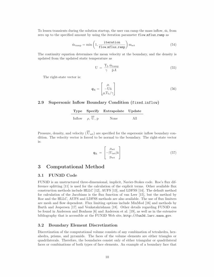
Figure 3. Perspective view of triangular boundary element in Y-Z plane.

Table 2. Boundary Element Node Weight Factors

Topology W1 W2 W3

Tetrahedral 6/8 1/8 1/8Hexahedral, prism, pyramid 1 0 0

consists of triangular face elements is shown in the perspective sketch in Figure 3. A spaceof subelements is formed to calculate the fluxes at the boundary. Three subelements areformed from each of the corner nodes (1, 2, and 3) of the triangular face element. The areaand the orientation of the quadrilateral subelements are determined by using the center ofthe element , Pc; the left and right midpoints, Pl and Pr; and the main node, Pm. Thenormal vector is the cross product of the two vectors that are formed from the main andcenter nodes,

−−−→PmPc, and the left and right midpoints,

−−→PlPr, so that �n =

−−−→PmPc ×−−→

PlPr.The interior, or left state, for the subelement is calculated from an area weighted average

of the interior state nodal values, q1, q2, and q3. The values of the area weights, W, changewith the element topology and are listed in Table 2. A detailed derivation of the boundarynode weighting for tetrahedral meshes can be found in appendix A.

qL = W1q1 + W2q2 + W3q3 (58)

A flux function calculates the contribution to the solution residual for the subelement fromthe interior and right-side (i.e., boundary condition ) states. The inviscid flux is added tothe solution residual at each solution time step. Roe’s approximate Riemann solver wasused for the boundary flux contributions to the residual.

4 Test Case Descriptions

The three geometries that are described in Sections 4.1 through 4.3 are used to demonstratethe inflow and outflow boundary conditions that were described in Section 2. The geometriesare representative of a typical physical situation that could be modeled with each of thedifferent boundary conditions. Static pressure and mass flow outflow subsonic conditions areapplied to the outflow boundary of the bell-mouth geometry, Section 4.1. Total pressure-total temperature conditions and mass flow inflow conditions are applied to the inflowboundary of the American Society Of Mechanical Engineers ( ASME ) nozzle geometry,

11

Section 4.2. Fixed primitive variable conditions that simulate a supersonic inflow are appliedto the inflow boundary of the diffuser geometry, Section 4.3.

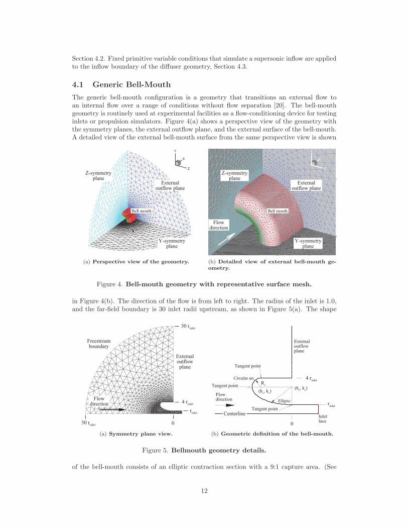
4.1 Generic Bell-Mouth

The generic bell-mouth configuration is a geometry that transitions an external flow toan internal flow over a range of conditions without flow separation [20]. The bell-mouthgeometry is routinely used at experimental facilities as a flow-conditioning device for testinginlets or propulsion simulators. Figure 4(a) shows a perspective view of the geometry withthe symmetry planes, the external outflow plane, and the external surface of the bell-mouth.A detailed view of the external bell-mouth surface from the same perspective view is shown

X

Y

Z

Bell mouth

Externaloutflow plane

Z-symmetryplane

Y-symmetryplane

(a) Perspective view of the geometry.

X

Y

Z

Bell mouth

Externaloutflow plane

Z-symmetryplane

Y-symmetryplane

Flowdirection

(b) Detailed view of external bell-mouth ge-ometry.

Figure 4. Bell-mouth geometry with representative surface mesh.

in Figure 4(b). The direction of the flow is from left to right. The radius of the inlet is 1.0,and the far-field boundary is 30 inlet radii upstream, as shown in Figure 5(a). The shape

rinlet

030 rinlet

4 rinlet

Externaloutflowplane

Flowdirection

Freestreamboundary

30 rinlet

(a) Symmetry plane view.

Circular arc

Ellipse

(hc, kc)(he, ke)

Tangent point

Tangent point

Flowdirection

Inletface

Externaloutflowplane

rinlet

0

4 rinlet

Centerline

Rc

Tangent point

(b) Geometric definition of the bell-mouth.

Figure 5. Bellmouth geometry details.

of the bell-mouth consists of an elliptic contraction section with a 9:1 capture area. (See

12

XY

Z

Y-symmetryplaneInflow

plane

Nozzlewall

Outflowplane

(a) Perspective view of the nozzle.

(hp, kp)×

Tangent points

(hn, kn)

Centerline

Flowdirection

Outflowplane

Inflowplane

Nozzlewall

0 8.0-10.0

(b) Geometric definition of the nozzle.

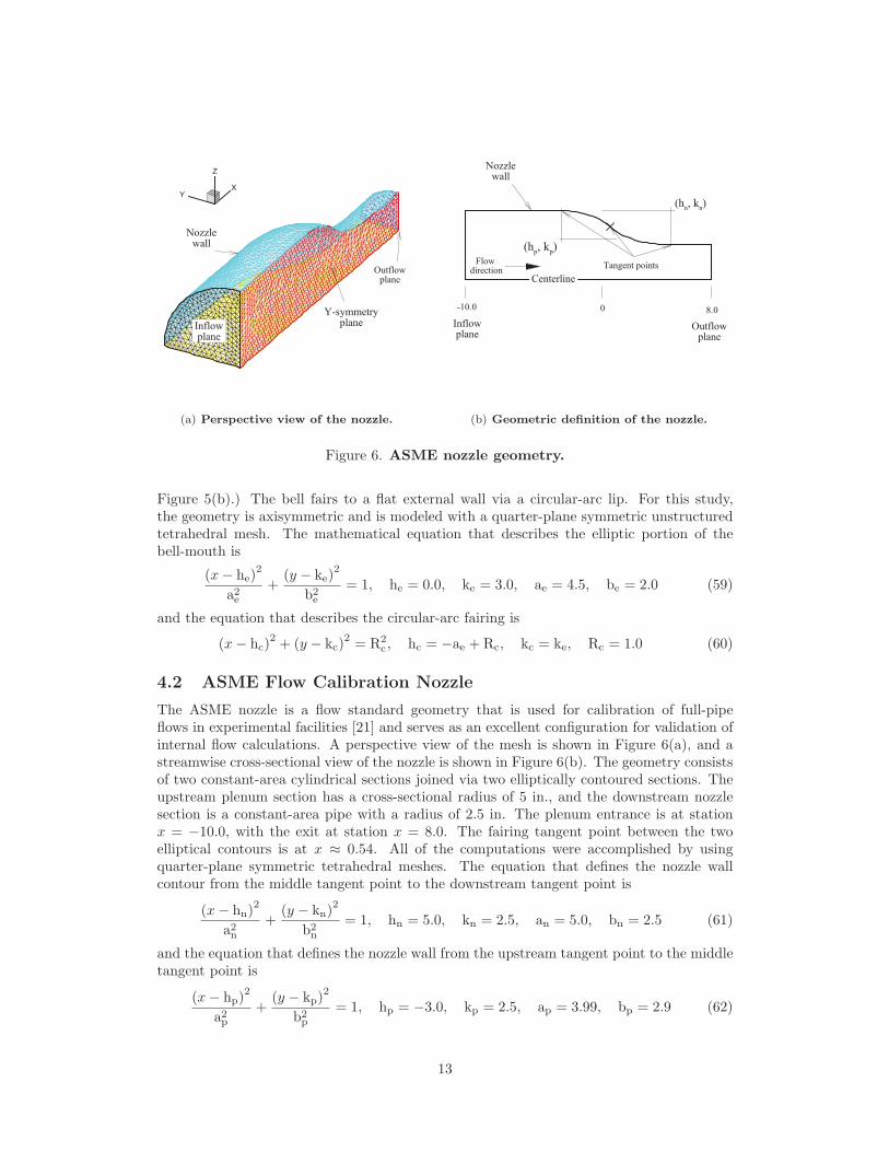
Figure 6. ASME nozzle geometry.

Figure 5(b).) The bell fairs to a flat external wall via a circular-arc lip. For this study,the geometry is axisymmetric and is modeled with a quarter-plane symmetric unstructuredtetrahedral mesh. The mathematical equation that describes the elliptic portion of thebell-mouth is

(x − he)2

a2e

+(y − ke)

2

b2e

= 1, he = 0.0, ke = 3.0, ae = 4.5, be = 2.0 (59)

and the equation that describes the circular-arc fairing is

(x − hc)2 + (y − kc)

2 = R2c , hc = −ae + Rc, kc = ke, Rc = 1.0 (60)

4.2 ASME Flow Calibration Nozzle

The ASME nozzle is a flow standard geometry that is used for calibration of full-pipeflows in experimental facilities [21] and serves as an excellent configuration for validation ofinternal flow calculations. A perspective view of the mesh is shown in Figure 6(a), and astreamwise cross-sectional view of the nozzle is shown in Figure 6(b). The geometry consistsof two constant-area cylindrical sections joined via two elliptically contoured sections. Theupstream plenum section has a cross-sectional radius of 5 in., and the downstream nozzlesection is a constant-area pipe with a radius of 2.5 in. The plenum entrance is at stationx = −10.0, with the exit at station x = 8.0. The fairing tangent point between the twoelliptical contours is at x ≈ 0.54. All of the computations were accomplished by usingquarter-plane symmetric tetrahedral meshes. The equation that defines the nozzle wallcontour from the middle tangent point to the downstream tangent point is

(x − hn)2

a2n

+(y − kn)2

b2n

= 1, hn = 5.0, kn = 2.5, an = 5.0, bn = 2.5 (61)

and the equation that defines the nozzle wall from the upstream tangent point to the middletangent point is

(x − hp)2

a2p

+(y − kp)2

b2p

= 1, hp = −3.0, kp = 2.5, ap = 3.99, bp = 2.9 (62)

13

XY

Z

Inflowplane

Diffuserwall

Y-symmetryplane

Outflowplane

Flowdirection

(a) Perspective view of the diffuser.

Inflowplane

Diffuserwall

Centerline

Outflowplane

Flowdirection 10.00

3°

(b) Geometric definition of the diffuser.

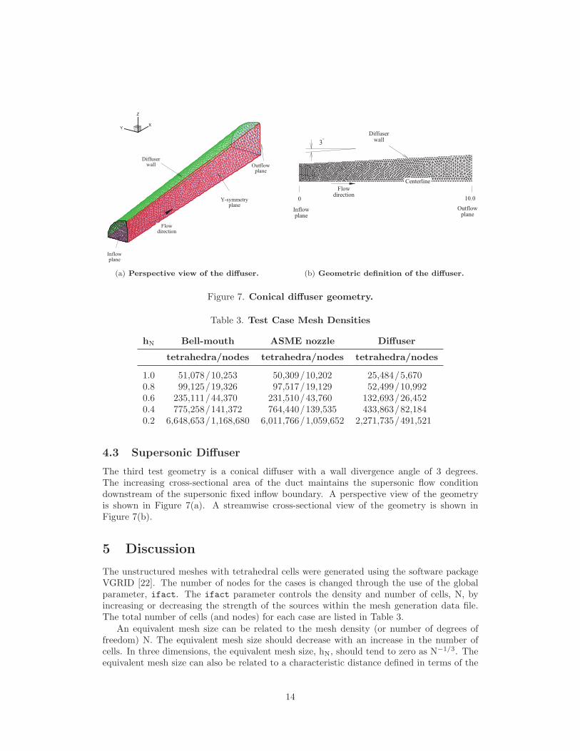
Figure 7. Conical diffuser geometry.

Table 3. Test Case Mesh Densities

hN Bell-mouth ASME nozzle Diffuser

tetrahedra/nodes tetrahedra/nodes tetrahedra/nodes

1.0 51,078/10,253 50,309/10,202 25,484/5,6700.8 99,125/19,326 97,517/19,129 52,499/10,9920.6 235,111/44,370 231,510/43,760 132,693/26,4520.4 775,258/141,372 764,440/139,535 433,863/82,1840.2 6,648,653/1,168,680 6,011,766/1,059,652 2,271,735/491,521

4.3 Supersonic Diffuser

The third test geometry is a conical diffuser with a wall divergence angle of 3 degrees.The increasing cross-sectional area of the duct maintains the supersonic flow conditiondownstream of the supersonic fixed inflow boundary. A perspective view of the geometryis shown in Figure 7(a). A streamwise cross-sectional view of the geometry is shown inFigure 7(b).

5 Discussion

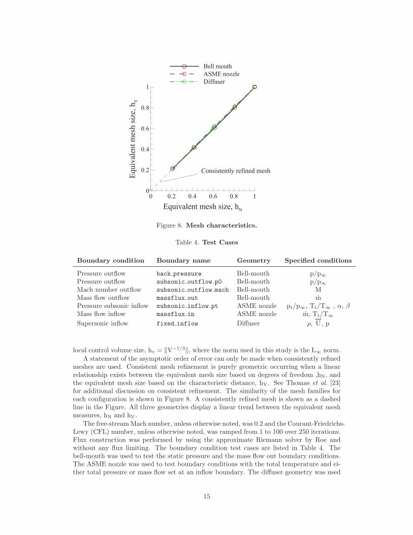
The unstructured meshes with tetrahedral cells were generated using the software packageVGRID [22]. The number of nodes for the cases is changed through the use of the globalparameter, ifact. The ifact parameter controls the density and number of cells, N, byincreasing or decreasing the strength of the sources within the mesh generation data file.The total number of cells (and nodes) for each case are listed in Table 3.

An equivalent mesh size can be related to the mesh density (or number of degrees offreedom) N. The equivalent mesh size should decrease with an increase in the number ofcells. In three dimensions, the equivalent mesh size, hN, should tend to zero as N−1/3. Theequivalent mesh size can also be related to a characteristic distance defined in terms of the

14

Equivalent mesh size, hN

Equi

vale

ntm

esh

size

,hV

0 0.2 0.4 0.6 0.8 10

0.2

0.4

0.6

0.8

1

Bell mouthASME nozzleDiffuser

Consistently refined mesh

Figure 8. Mesh characteristics.

Table 4. Test Cases

Boundary condition Boundary name Geometry Specified conditions

Pressure outflow back pressure Bell-mouth p/p∞Pressure outflow subsonic outflow p0 Bell-mouth p/p∞Mach number outflow subsonic outflow mach Bell-mouth MMass flow outflow massflux out Bell-mouth mPressure subsonic inflow subsonic inflow pt ASME nozzle pt/p∞, Tt/T∞ , α, βMass flow inflow massflux in ASME nozzle m, Tt/T∞Supersonic inflow fixed inflow Diffuser ρ,

−→U, p

local control volume size, hv = ‖V−1/3‖, where the norm used in this study is the L∞ norm.A statement of the asymptotic order of error can only be made when consistently refined

meshes are used. Consistent mesh refinement is purely geometric occurring when a linearrelationship exists between the equivalent mesh size based on degrees of freedom ,hN, andthe equivalent mesh size based on the characteristic distance, hV. See Thomas et al. [23]for additional discussion on consistent refinement. The similarity of the mesh families foreach configuration is shown in Figure 8. A consistently refined mesh is shown as a dashedline in the Figure. All three geometries display a linear trend between the equivalent meshmeasures, hN and hV.

The free-stream Mach number, unless otherwise noted, was 0.2 and the Courant-Friedrichs-Lewy (CFL) number, unless otherwise noted, was ramped from 1 to 100 over 250 iterations.Flux construction was performed by using the approximate Riemann solver by Roe andwithout any flux limiting. The boundary condition test cases are listed in Table 4. Thebell-mouth was used to test the static pressure and the mass flow out boundary conditions.The ASME nozzle was used to test boundary conditions with the total temperature and ei-ther total pressure or mass flow set at an inflow boundary. The diffuser geometry was used

15

Mach

0.320.300.270.250.230.210.180.160.140.110.090.070.050.020.00

M∞

Figure 9. Mach number contours for the bell-mouth geometry.

to test the supersonic fixed inflow boundary condition. In the following sections, solutionconvergence histories for each of the mesh densities are shown for each boundary condi-tion. Also, the convergence of the error in the boundary value is shown for each boundarycondition. The error in the boundary condition is the difference between the user-definedboundary condition and the area-weighted average of the boundary solution condition fromthe code. The area-weighted average for a variable, φ, is designated by an overbar φ and iscalculated as

∫boundary

φdA/∫boundary

dA.The area-weighted average values for ρ, p, pt, and mass flow are calculated by the

summation equations, Eqs. (63). The average velocity, speed of sound, and Mach numberare calculated by Eqs. (64).

ρ =1A

∑boundary

ρ δA, p =1A

∑boundary

p δA, pt =1A

∑boundary

(p +

12ρU2

)δA (63)

m =∑

boundary

ρU⊥δA, U = m/ρA, c =√

γp/ρ, M = U/c (64)

where δA is the area of an individual element on the boundary face and A is the boundaryarea, A =

∑boundary δA. The error in the boundary condition for the parameter φ is then

Errorφ = φset − φ (65)

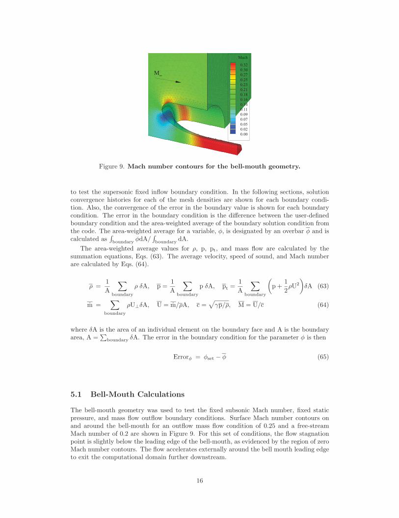
5.1 Bell-Mouth Calculations

The bell-mouth geometry was used to test the fixed subsonic Mach number, fixed staticpressure, and mass flow outflow boundary conditions. Surface Mach number contours onand around the bell-mouth for an outflow mass flow condition of 0.25 and a free-streamMach number of 0.2 are shown in Figure 9. For this set of conditions, the flow stagnationpoint is slightly below the leading edge of the bell-mouth, as evidenced by the region of zeroMach number contours. The flow accelerates externally around the bell mouth leading edgeto exit the computational domain further downstream.

16

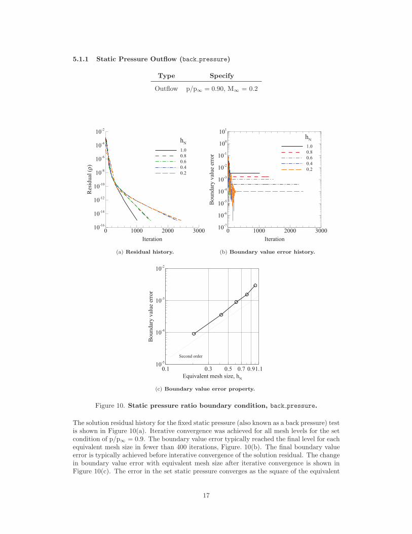
5.1.1 Static Pressure Outflow (back pressure)

Type Specify

Outflow p/p∞ = 0.90, M∞ = 0.2

Iteration

Res

idua

l(ρ)

0 1000 2000 300010-16

10-14

10-12

10-10

10-8

10-6

10-4

10-2

1.00.80.60.40.2

hN

(a) Residual history.

Iteration

Bou

ndar

yva

lue

erro

r

0 1000 2000 300010-7

10-6

10-5

10-4

10-3

10-2

10-1

100

101

1.00.80.60.40.2

hN

(b) Boundary value error history.


Bou

ndar

yva

lue

erro

r

0.1 0.3 0.5 0.7 0.91.110-5

10-4

10-3

10-2

Second order

(c) Boundary value error property.

Figure 10. Static pressure ratio boundary condition, back pressure.

The solution residual history for the fixed static pressure (also known as a back pressure) testis shown in Figure 10(a). Iterative convergence was achieved for all mesh levels for the setcondition of p/p∞ = 0.9. The boundary value error typically reached the final level for eachequivalent mesh size in fewer than 400 iterations, Figure. 10(b). The final boundary valueerror is typically achieved before interative convergence of the solution residual. The changein boundary value error with equivalent mesh size after iterative convergence is shown inFigure 10(c). The error in the set static pressure converges as the square of the equivalent

17

mesh size. The second-order convergence property in the error is indicated by the slope ofthe dotted line.

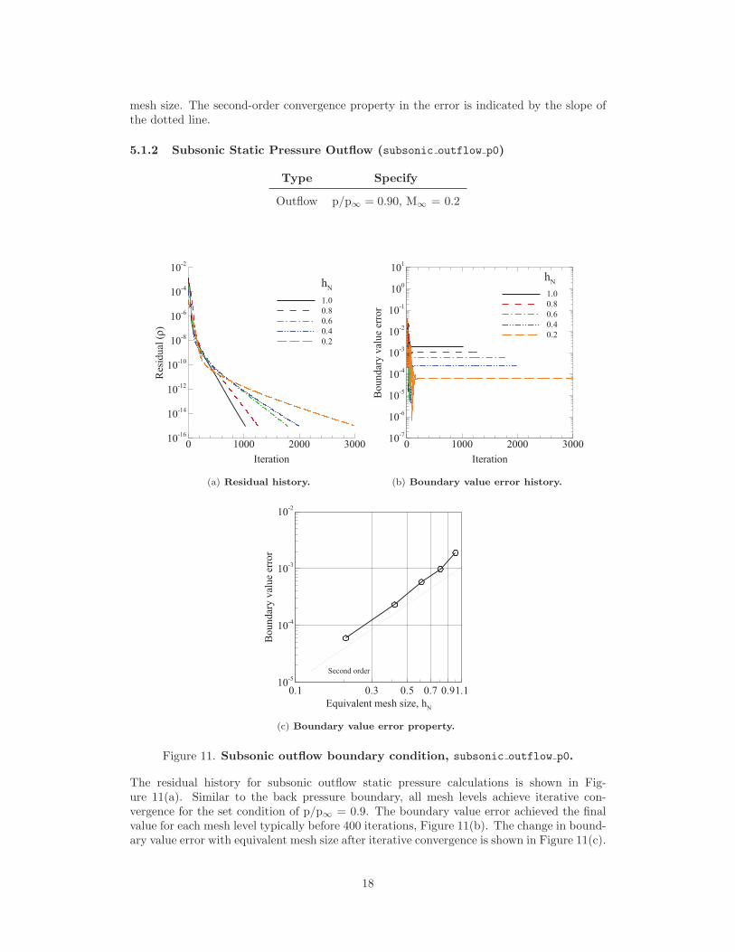
5.1.2 Subsonic Static Pressure Outflow (subsonic outflow p0)

Type Specify

Outflow p/p∞ = 0.90, M∞ = 0.2

Iteration

Res

idua

l(ρ)

0 1000 2000 300010-16

10-14

10-12

10-10

10-8

10-6

10-4

10-2

1.00.80.60.40.2

hN


Iteration

Bou

ndar

yva

lue

erro

r

0 1000 2000 300010-7

10-6

10-5

10-4

10-3

10-2

10-1

100

101

1.00.80.60.40.2

hN



Bou

ndar

yva

lue

erro

r

0.1 0.3 0.5 0.7 0.91.110-5

10-4

10-3

10-2

Second order


Figure 11. Subsonic outflow boundary condition, subsonic outflow p0.

The residual history for subsonic outflow static pressure calculations is shown in Fig-ure 11(a). Similar to the back pressure boundary, all mesh levels achieve iterative con-vergence for the set condition of p/p∞ = 0.9. The boundary value error achieved the finalvalue for each mesh level typically before 400 iterations, Figure 11(b). The change in bound-ary value error with equivalent mesh size after iterative convergence is shown in Figure 11(c).

18

The error in the set static pressure converges as the square of the equivalent mesh size. Thesecond-order convergence property in the error is indicated by the slope of the dotted line.

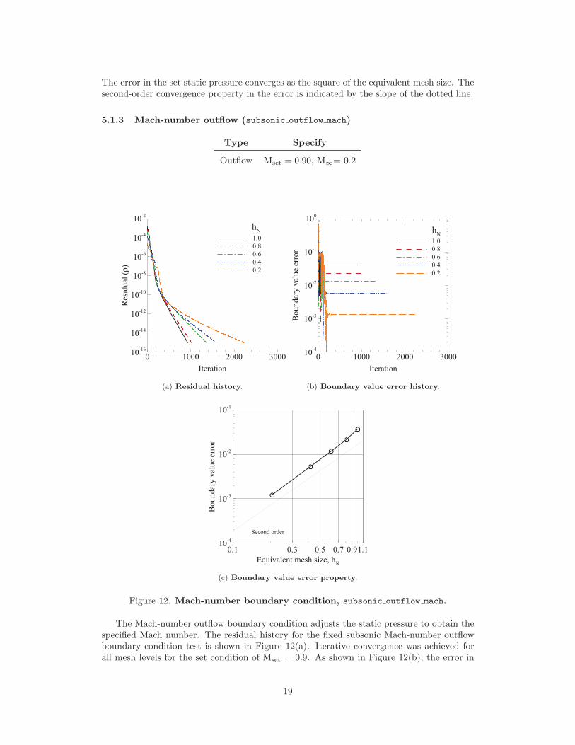
5.1.3 Mach-number outflow (subsonic outflow mach)

Type Specify

Outflow Mset = 0.90, M∞= 0.2

Iteration

Res

idua

l(ρ)

0 1000 2000 300010-16

10-14

10-12

10-10

10-8

10-6

10-4

10-2

1.00.80.60.40.2

hN


Iteration

Bou

ndar

yva

lue

erro

r

0 1000 2000 300010-4

10-3

10-2

10-1

100

1.00.80.60.40.2

hN



Bou

ndar

yva

lue

erro

r

0.1 0.3 0.5 0.7 0.91.110-4

10-3

10-2

10-1

Second order


Figure 12. Mach-number boundary condition, subsonic outflow mach.

The Mach-number outflow boundary condition adjusts the static pressure to obtain thespecified Mach number. The residual history for the fixed subsonic Mach-number outflowboundary condition test is shown in Figure 12(a). Iterative convergence was achieved forall mesh levels for the set condition of Mset = 0.9. As shown in Figure 12(b), the error in

19

the Mach number reaches the final value within several hundred iterations for this test case.The error in the set Mach number converges as the square of the equivalent mesh size. Thesecond-order convergence property in the error is indicated by the slope of the dotted line(Figure 12(c)). For this configuration, Mset= 0.9 is approximately equivalent to a inflowstatic pressure ratio of p/p∞ = 0.61.

5.1.4 Mass flow outflow (massflux out)

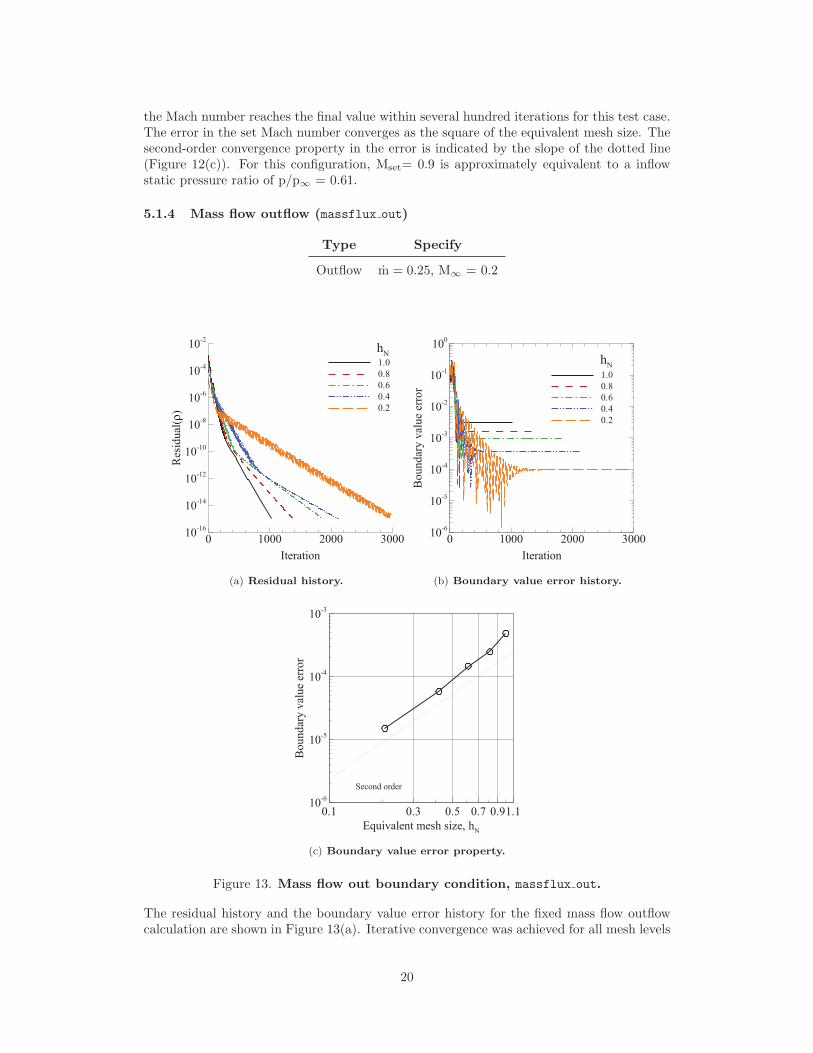
Type Specify

Outflow m = 0.25, M∞ = 0.2

Iteration

Res

idua

l(ρ)

0 1000 2000 300010-16

10-14

10-12

10-10

10-8

10-6

10-4

10-2

1.00.80.60.40.2

hN


Iteration

Bou

ndar

yva

lue

erro

r

0 1000 2000 300010-6

10-5

10-4

10-3

10-2

10-1

100

1.00.80.60.40.2

hN



Bou

ndar

yva

lue

erro

r

0.1 0.3 0.5 0.7 0.91.110-6

10-5

10-4

10-3

Second order


Figure 13. Mass flow out boundary condition, massflux out.

The residual history and the boundary value error history for the fixed mass flow outflowcalculation are shown in Figure 13(a). Iterative convergence was achieved for all mesh levels

20

for the set condition of m = 0.25. As shown in Figure 13(b), the error in the mass flowreaches the final value within several hundred iterations for most cases. The relaxation ofthe static pressure to set the mass flow took longer for the equivalent size mesh hN = 0.2as a result of a lower damping of the pressure oscillations in the flow field. The error inthe set mass flow converges as the square of the equivalent mesh size. The second-orderconvergence property in the error is indicated by the slope of the dotted line (Figure 13(c)).The average values for the Mach number and the static pressure ratio at the boundary forthis mass flow setting are approximately 0.33 and 0.95, respectively.

5.2 ASME Nozzle Calculations

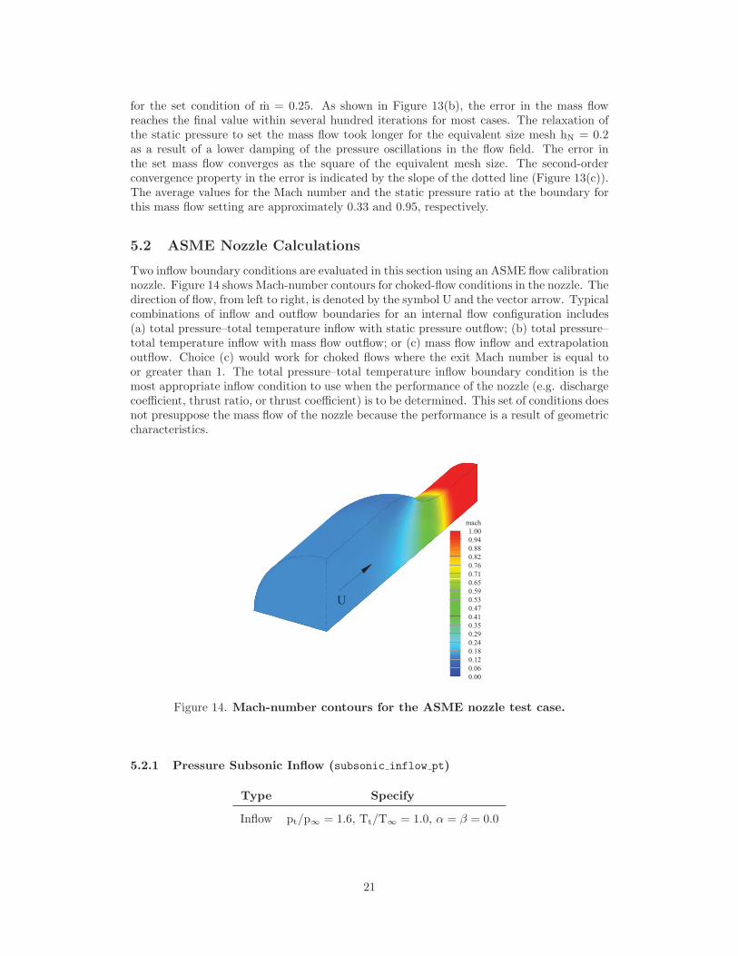
Two inflow boundary conditions are evaluated in this section using an ASME flow calibrationnozzle. Figure 14 shows Mach-number contours for choked-flow conditions in the nozzle. Thedirection of flow, from left to right, is denoted by the symbol U and the vector arrow. Typicalcombinations of inflow and outflow boundaries for an internal flow configuration includes(a) total pressure–total temperature inflow with static pressure outflow; (b) total pressure–total temperature inflow with mass flow outflow; or (c) mass flow inflow and extrapolationoutflow. Choice (c) would work for choked flows where the exit Mach number is equal toor greater than 1. The total pressure–total temperature inflow boundary condition is themost appropriate inflow condition to use when the performance of the nozzle (e.g. dischargecoefficient, thrust ratio, or thrust coefficient) is to be determined. This set of conditions doesnot presuppose the mass flow of the nozzle because the performance is a result of geometriccharacteristics.

mach1.000.940.880.820.760.710.650.590.530.470.410.350.290.240.180.120.060.00

U

Figure 14. Mach-number contours for the ASME nozzle test case.

5.2.1 Pressure Subsonic Inflow (subsonic inflow pt)

Type Specify

Inflow pt/p∞ = 1.6, Tt/T∞ = 1.0, α = β = 0.0

21

Iteration

Res

idua

l(ρ)

0 500 1000 150010-16

10-14

10-12

10-10

10-8

10-6

10-4

10-2

1.00.80.60.40.2

hN


Iteration

Bou

ndar

yva

lue

erro

r

0 500 1000 150010-8

10-7

10-6

10-5

10-4

10-3

10-2

10-1

100

1.00.80.60.40.2

hN



Bou

ndar

yva

lue

erro

r

0.1 0.3 0.5 0.7 0.91.110-7

10-6

10-5

10-4

Second order


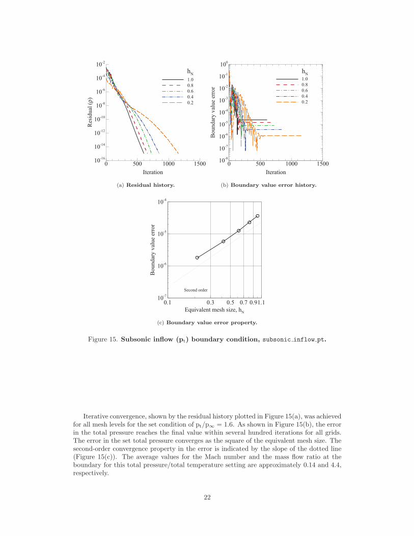
Figure 15. Subsonic inflow (pt) boundary condition, subsonic inflow pt.

Iterative convergence, shown by the residual history plotted in Figure 15(a), was achievedfor all mesh levels for the set condition of pt/p∞ = 1.6. As shown in Figure 15(b), the errorin the total pressure reaches the final value within several hundred iterations for all grids.The error in the set total pressure converges as the square of the equivalent mesh size. Thesecond-order convergence property in the error is indicated by the slope of the dotted line(Figure 15(c)). The average values for the Mach number and the mass flow ratio at theboundary for this total pressure/total temperature setting are approximately 0.14 and 4.4,respectively.

22

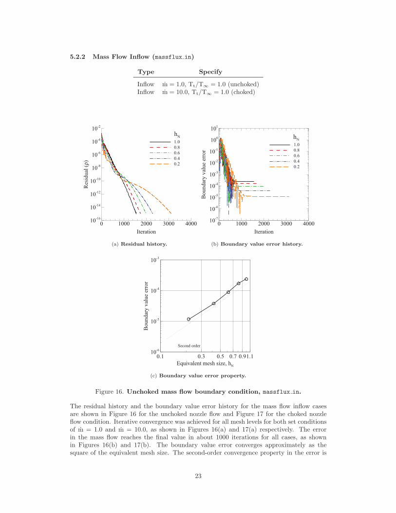
5.2.2 Mass Flow Inflow (massflux in)

Type Specify

Inflow m = 1.0, Tt/T∞ = 1.0 (unchoked)Inflow m = 10.0, Tt/T∞ = 1.0 (choked)

Iteration

Res

idua

l(ρ)

0 1000 2000 3000 400010-16

10-14

10-12

10-10

10-8

10-6

10-4

10-2

1.00.80.60.40.2

hN


Iteration

Bou

ndar

yva

lue

erro

r

0 1000 2000 3000 400010-7

10-6

10-5

10-4

10-3

10-2

10-1

100

101

1.00.80.60.40.2

hN



Bou

ndar

yva

lue

erro

r

0.1 0.3 0.5 0.7 0.91.110-6

10-5

10-4

10-3

Second order


Figure 16. Unchoked mass flow boundary condition, massflux in.

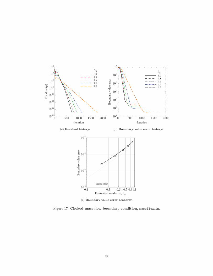
The residual history and the boundary value error history for the mass flow inflow casesare shown in Figure 16 for the unchoked nozzle flow and Figure 17 for the choked nozzleflow condition. Iterative convergence was achieved for all mesh levels for both set conditionsof m = 1.0 and m = 10.0, as shown in Figures 16(a) and 17(a) respectively. The errorin the mass flow reaches the final value in about 1000 iterations for all cases, as shownin Figures 16(b) and 17(b). The boundary value error converges approximately as thesquare of the equivalent mesh size. The second-order convergence property in the error is

23

Iteration

Res

idua

l(ρ)

0 500 1000 1500 200010-16

10-14

10-12

10-10

10-8

10-6

10-4

10-2

1.00.80.60.40.2

hN


Iteration

Bou

ndar

yva

lue

erro

r

0 500 1000 1500 200010-6

10-5

10-4

10-3

10-2

10-1

100

1.00.80.60.40.2

hN



Bou

ndar

yva

lue

erro

r

0.1 0.3 0.5 0.7 0.91.110-6

10-5

10-4

10-3

Second order


Figure 17. Choked mass flow boundary condition, massflux in.

24

indicated by the slope of the dotted line (Figures 16(c) and 17(c)). The average values forthe total pressure ratio at the inflow boundary for the unchoked and choked nozzle massflow conditions are approximately 1.03 and 3.5, respectively.

5.3 Supersonic Diffuser Calculations

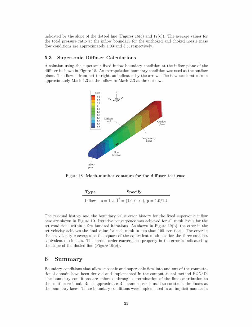
A solution using the supersonic fixed inflow boundary condition at the inflow plane of thediffuser is shown in Figure 18. An extrapolation boundary condition was used at the outflowplane. The flow is from left to right, as indicated by the arrow. The flow accelerates fromapproximately Mach 1.3 at the inflow to Mach 2.3 at the outflow.

XY

Zmach

2.32.22.121.91.81.71.61.51.41.3

Inflowplane

Diffuserwall

Y-symmetryplane

Outflowplane

Flowdirection

Figure 18. Mach-number contours for the diffuser test case.

Type Specify

Inflow ρ = 1.2,−→U = (1.0, 0., 0.), p = 1.0/1.4

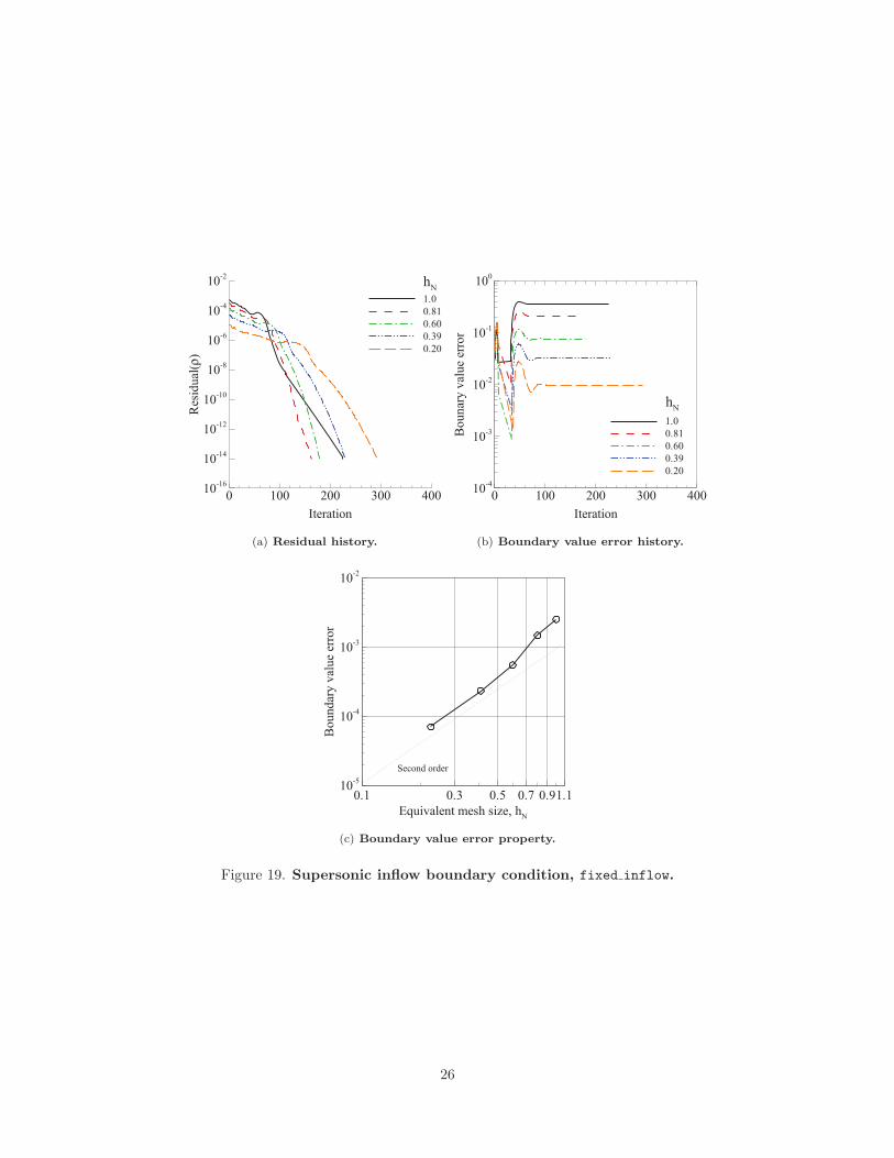
The residual history and the boundary value error history for the fixed supersonic inflowcase are shown in Figure 19. Iterative convergence was achieved for all mesh levels for theset conditions within a few hundred iterations. As shown in Figure 19(b), the error in theset velocity achieves the final value for each mesh in less than 100 iterations. The error inthe set velocity converges as the square of the equivalent mesh size for the three smallestequivalent mesh sizes. The second-order convergence property in the error is indicated bythe slope of the dotted line (Figure 19(c)).

6 Summary

Boundary conditions that allow subsonic and supersonic flow into and out of the computa-tional domain have been derived and implemented in the computational method FUN3D.The boundary conditions are enforced through determination of the flux contribution tothe solution residual. Roe’s approximate Riemann solver is used to construct the fluxes atthe boundary faces. These boundary conditions were implemented in an implicit manner in

25

Iteration

Res

idua

l(ρ)

0 100 200 300 40010-16

10-14

10-12

10-10

10-8

10-6

10-4

10-2

1.00.810.600.390.20

hN


Iteration

Bou

nary

valu

eer

ror

0 100 200 300 40010-4

10-3

10-2

10-1

100

1.00.810.600.390.20

hN



Bou

ndar

yva

lue

erro

r

0.1 0.3 0.5 0.7 0.91.110-5

10-4

10-3

10-2

Second order


Figure 19. Supersonic inflow boundary condition, fixed inflow.

26

the FUN3D CFD code and were verified for three generic test geometries. Iterative residualconvergence was achieved at all mesh-density levels for all of the conditions that were used inthis study. The user-requested condition was achieved in all cases, and error in the bound-ary condition value decreased in a second-order manner with an increase in mesh density.Boundary value error convergence occurs before iterative convergence and depending on theapplication, boundary values were within 0.5 percent of the specified parameter value withonly a residual reduction of 5 orders of magnitude.

Acknowledegment

The author would like to thank Dr. James Thomas, Dr. Mike Park and Mr. Jeff White ofthe Computational AeroSciences Branch at NASA Langley Research Center for their manyinvaluable discussions and contributions to this work.

7 Nomenclature

Roman lettersA areac speed of soundcp specific heat at constant pressureH enthalpyhN equivalent mesh size based on degrees of freedom, N−1/3

hv L1 norm of V−1/3, |L1| = ‖V−1/3‖1

i, j, k Cartesian unit vectors axis in physical spacem mass flowM Mach number�n normal vectorn unit normal vector, �n/|�n|N number of nodes in meshp static pressureR real gas constantR Riemann invariants entropyT temperatureU average velocity−→U velocity vector, [u, v, w]T

U velocity magnitudeu,v,w Cartesian velocity componentsV primal volume of elements in meshx, y, z Cartesian coordinates in physical space

Subscriptsb boundary state∞ free-stream statei internal stateL left state

27

o outer state⊥ normal to boundary elementR right stateset user-requested conditiont total conditions

ConventionsF boundary element flux vectorq primitive variables state vectorR solution residual vector

Symbolsα u-w angle of velocityβ u-v angle of velocityγ ratio of specific heats, γ = 1.4 (air)λ eigenvalueρ density

References

1. “Numerical Boundary Condition Procedures,” Symposium on Numerical BoundaryCondition Procedures, ed. P. Kutler, NASA CP–2201, October 1981.

2. Moretti, G.: “A Physical Approach to the Numerical Treatment of Boundaries in GasDynamics,” NASA CP–2201, October 1981, pp. 73–95.

3. Blottner, F.: “Influence of Boundary Approximations and Conditions on Finite Differ-ence Solutions,” NASA CP–2201, October 1981, pp. 227–256.

4. Pulliam, T.: “Characteristic Boundary Conditions for the Euler Equations,” NASACP–2201, October 1981, pp. 165–181.

5. Thompkins, W. and Bush, R.: “Boundary Treatments for Implicit Solutions to Eulerand Navier-Stokes Equations,” NASA CP–2201, October 1981, pp. 353–363.

6. Anderson, W. and Bonhaus, D. L.: “An Implicit Upwind Algorithm for ComputingTurbulent Flows on Unstructed Grids,” Computers & Fluids, Vol. 23, 1994, pp. 1–21.

7. Kim, S.; Alonso, J.; Schluter, J.; Wu, X. and Pitsch, H.: “Integrated Simulationsfor Multi-Component Analysis of Gas Turbines: RANS Boundary Conditions,” AIAAPaper 2004-3415, July 2004.

8. Griewank, A.: “On Automatic Differentiation,” Mathematical Programming: RecentDevelopments and Applications, Kluwer Academic Publishers, 1989, pp. 83–108.

9. Corliss, G. F. and Griewank, A.: “Operator Overloading as an Enabling Technology forAutomatic Differentiation,” Technical report, Argonne National Laboratory, 1993.

10. White, J. and Morrison, J.: “A Pseudo-Temporal Multi-Grid Relaxation Scheme forSolving the Parabolized Navier-Stokes Equations,” AIAA Paper 1999-3360, June 1999.

11. Roe, P. L.: “Approximate Riemann Solvers, Parameter Vectors, and DifferenceSchemes,” J. Comp. Phys., Vol. 43, 1981, pp. 357–372.

28

12. Batten, P.; Clarke, N.; Lambert, C. and Causon, D.: “On the Choice of Wavespeeds forthe HCCL Riemann Solver,” SIAM J. Sci. Comput., Vol. 18, 1997, pp. 1553–1570.

13. Sun, M. and Takayama, K.: “Artificially Upwind Flux Vector Splitting Scheme for theEuler Equations,” J. Comp. Phys., Vol. 189, 2003, pp. 305–329.

14. Edwards, J.: “A Low-Diffusion Flux-Splitting Scheme for Navier Stokes Calculations,”AIAA Paper 1996-1704, May 1996.

15. van Leer, B.: “Towards the Ultimate Conservative Difference Schemes V. A secondOrder Sequel to Godunov’s Method,” J. Comp. Phys., Vol. 32, 1979, pp. 101–136.

16. Roe, P. L.: “Characteristic-Based Schemes for the Euler Equations,” Annual Review ofFluid Mechanics, Vol. 18, 1986, pp. 337–365.

17. Barth, T. and Jespersen, D.: “The Design and Application of Upwind Schemes onUnstructured Meshes,” AIAA Paper 1989-0366, Jan. 1989.

18. Venkatakrishnan, V.: “Convergence to Steady State Solutions of the Euler Equationson Unstructured Grids with Limiters,” J. Comp. Phys., Vol. 118, 1995, pp. 120–130.

19. Anderson, W.; Rausch, R. and Bonhaus, D. L.: “Implicit/Multigrid Algorithms forIncompressible Turbulent Flows on Unstructured Grids,” J. Comp. Phys, Vol. 128,1996, pp. 391–408.

20. Gilbert, G. and Hill, P.: “Analysis and Testing of Two-Dimensional Slot Nozzle EjectorsWith Variable Area Mixing Sections,” NASA CR–2251, May 1973.

21. Measurement of Fluid Flow in Pipes Using Orifice, Nozzle and Venturi, The AmericanSociety of Mechanical Engineers, 2005.

22. Pirzadeh, S.: “Three-Dimensional Unstructured Viscous Grids by the Advancing-LayersMethod,” AIAA Journal, Vol. 34, No. 1, 1996, pp. 43–49.

23. Thomas, J.; Diskin, B. and Rumsey, C.: “Toward Verification of Unstructured-GridSolvers,” AIAA Journal, Vol. 46, No. 12, 2008, pp. 3070–3079.

29

Appendix A

Node Weighting for a Boundary Tetrahedral

The tetrahedral element that is shown in Figure A1 has four nodes with an associatedarea-weighted normal, �n1, �n2, �n3, and �n4, opposite each node. The average value of the

XY

Z Node 4

Node 1

Node 3

Node 2

tetrahedral cell

n2

n3

n1

n4

→

→

→

→

Figure A1. Tetrahedral element.

variable qi at the face centers is one-third the sum of the three corners of that face if weassume that a constant gradient exists across the element.

q1 =13

(qnode2 + qnode3 + qnode4) (A1)

q2 =13


q3 =13


q4 =13


The Green-Gauss (GG) integral over the tetrahedral element is equal to one-third the sum-mation of the product of the average value of qi with each directed face normal, �ni.

∮ GG

tetrahedron

∇qdV =13

4∑i=1

qi�ni (A5)

The dual of the tetrahedral element shown in Figure A2 has six faces, with the associatednormals �nB, �nL, and �nR on the boundaries and �n12, �n13, and �n14 facing the tetrahedral faceopposite node 1. The finite-volume (FV) integral around the dual volume is written as asummation of q times the directed normal of the face. At this point, the influence of thenodes on the boundary faces L, R, B, a, b, and c are unknown. The goal is to make the FV

30

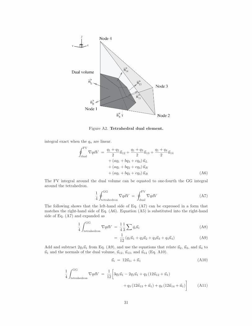
Figure A2. Tetrahedral dual element.

integral exact when the qn are linear.∮ FV

dual

∇qdV =q1 + q2

2�n12 +

q1 + q3

2�n13 +

q1 + q4

2�n14

+ (aq1 + bq3 + cq4)�nL

+ (aq1 + bq2 + cq4)�nR

+ (aq1 + bq2 + cq3)�nB (A6)

The FV integral around the dual volume can be equated to one-fourth the GG integralaround the tetrahedron.

14

∮ GG

tetrahedron

∇qdV =∮ FV

dual

∇qdV (A7)

The following shows that the left-hand side of Eq. (A7) can be expressed in a form thatmatches the right-hand side of Eq. (A6). Equation (A5) is substituted into the right-handside of Eq. (A7) and expanded as

14

∫ GG

tetrahedron

∇qdV =14

13

∑qi�ni (A8)

=112

(q1�n1 + q2�n2 + q3�n3 + q4�n4) (A9)

Add and subtract 2q1�n1 from Eq. (A9), and use the equations that relate �n2, �n3, and �n4 to�n1 and the normals of the dual volume, �n12, �n13, and �n14 (Eq. A10).

�ni = 12�n1i + �n1 (A10)

14

∫ GG

tetrahedron

∇qdV =112

[3q1�n1 − 2q1�n1 + q2 (12�n12 + �n1)

+ q3 (12�n13 + �n1) + q4 (12�n14 + �n1)]

(A11)

31

Split the terms with the �n1i normal vector as

14

∫ GG

tetrahedron

∇qdV =112

[−2q1�n1 + 6q2�n12 + 6q3�n13 + 6q4�n14

+ 3q1�n1 + q2�n1 + q3�n1 + q4�n1

+ 6q2�n12 + 6q3�n13 + 6q4�n14

](A12)

Substituting into Eq. (A12) the additional geometric relations that equate the face normalsof �n1, �n12, �n13, and �n14 with �nL, �nR, and �nB (Eqs. (A13)-(A16):

�n1 = −3 (�n12 + �n13 + �n14) = 3 (�nL + �nR + �nB) (A13)

�n12 = −14

(2�nL + �nR + �nB) (A14)

�n13 = −14

(�nL + 2�nR + �nB) (A15)

�n14 = −14

(�nL + �nR + 2�nB) (A16)

14

∫ GG

tetrahedron

∇qdV =q1 + q2

2�n12 +

q1 + q3

2�n13 +

q1 + q4

2�n14 +

112

(3q1�n1)

+ q2

[−1

8(2�nL + �nR + �nB) +

14

(�nL + �nR + �nB)]

+ q3

[−1

8(�nL + 2�nR + �nB) +

14

(�nL + �nR + �nB)]

+ q4

[−1

8(�nL + �nR + 2�nB) +

14

(�nL + �nR + �nB)]

(A17)

Finally, gather terms of similar face vectors:

14

∫ GG

tetrahedron

∇qdV =q1 + q2

2�n12 +

q1 + q3

2�n13 +

q1 + q4

2�n14

+(

34q1 +

18q3 +

18q4

)�nL

+(

34q1 +

18q2 +

18q4

)�nR

+(

34q1 +

18q2 +

18q3

)�nB (A18)

A direct comparison of the terms in Eq. (A18) with those in Eq. (A6) shows that a = 3/4,b = 1/8, and c = 1/8.

The author would like to thank Nishikawa Hiroaki for this derivation.

32

REPORT DOCUMENTATION PAGE Form ApprovedOMB No. 0704-0188

2. REPORT TYPE Technical Memorandum

4. TITLE AND SUBTITLE


5a. CONTRACT NUMBER

6. AUTHOR(S)

Carlson, Jan-Renee

7. PERFORMING ORGANIZATION NAME(S) AND ADDRESS(ES)NASA Langley Research CenterHampton, VA 23681-2199

9. SPONSORING/MONITORING AGENCY NAME(S) AND ADDRESS(ES)National Aeronautics and Space AdministrationWashington, DC 20546-0001

8. PERFORMING ORGANIZATION REPORT NUMBER

L-20011

10. SPONSOR/MONITOR'S ACRONYM(S)

NASA

13. SUPPLEMENTARY NOTES

12. DISTRIBUTION/AVAILABILITY STATEMENTUnclassified UnlimitedSubject Category 64 Availability: NASA CASI (443) 757-5802

19a. NAME OF RESPONSIBLE PERSON

STI Help Desk (email: [email protected])

14. ABSTRACT

Several boundary conditions that allow subsonic and supersonic flow into and out of the computational domain are discussed. These boundary conditions are demonstrated in the FUN3D computational fluid dynamics (CFD) code which solves the three-dimensional Navier-Stokes equations on unstructured computational meshes. The boundary conditions are enforced through determination of the flux contribution at the boundary to the solution residual. The boundary conditions are implemented in an implicit form where the Jacobian contribution of the boundary condition is included and is exact. All of the flows are governed by the calorically perfect gas thermodynamic equations. Three problems are used to assess these boundary conditions. Solution residual convergence to machine zero precision occurred for all cases. The converged solution boundary state is compared with the requested boundary state for several levels of mesh densities. The boundary values convergedto the requested boundary condition with approximately second-order accuracy for all of the cases.15. SUBJECT TERMS

CFD, unstructured mesh, euler, boundary conditions, propulsion simulation18. NUMBER OF PAGES

3819b. TELEPHONE NUMBER (Include area code)

(443) 757-5802

a. REPORT

U

c. THIS PAGE

U

b. ABSTRACT

U

17. LIMITATION OF ABSTRACT

UU

Prescribed by ANSI Std. Z39.18Standard Form 298 (Rev. 8-98)

3. DATES COVERED (From - To)01/2005-12/2008

5b. GRANT NUMBER

5c. PROGRAM ELEMENT NUMBER

5d. PROJECT NUMBER

5e. TASK NUMBER

5f. WORK UNIT NUMBER

11. SPONSOR/MONITOR'S REPORT NUMBER(S)

NASA/TM-2011-217181

16. SECURITY CLASSIFICATION OF:

The public reporting burden for this collection of information is estimated to average 1 hour per response, including the time for reviewing instructions, searching existing data sources, gathering and maintaining the data needed, and completing and reviewing the collection of information. Send comments regarding this burden estimate or any other aspect of this collection of information, including suggestions for reducing this burden, to Department of Defense, Washington Headquarters Services, Directorate for Information Operations and Reports (0704-0188), 1215 Jefferson Davis Highway, Suite 1204, Arlington, VA 22202-4302. Respondents should be aware that notwithstanding any other provision of law, no person shall be subject to any penalty for failing to comply with a collection of information if it does not display a currently valid OMB control number.PLEASE DO NOT RETURN YOUR FORM TO THE ABOVE ADDRESS.

1. REPORT DATE (DD-MM-YYYY)10 - 201101-

inflow/outflow boundary conditions with application … · 10.01.2011 · inflow/outflow boundary...

Documents