on simulation of outflow boundary conditions in finite ...molshan/ftp/pub/outflow.pdf · on...

INTERNATIONAL JOURNAL FOR NUMERICAL METHODS IN FLUIDSInt. J. Numer. Meth. Fluids 2000; 33: 499–534

On simulation of outflow boundary conditions in finitedifference calculations for incompressible fluid

M. A. Ol’shanskii* and V. M. Staroverov

Department of Mechanics and Mathematics, Moscow State Uni6ersity, Moscow, Russian Federation

SUMMARY

For incompressible Navier–Stokes equations in primitive variables, a method of setting absorbingoutflow boundary conditions on an artificial boundary is considered. The advection equations used onthe outflow boundary are convenient for finite difference (FD) methods, where a weak formulation of aproblem is inapplicable. An unsteady viscous incompressible Navier–Stokes flow in a channel with amoving damper is modeled. An accurate comparison and analysis of numerical and mechanical situationsare carried out for a variety of boundary conditions and Reynolds numbers. The proposed outflowconditions provide that the problem with Dirichlet boundary conditions should be solved on each timestep. Copyright © 2000 John Wiley & Sons, Ltd.

KEY WORDS: artificial boundary; finite differences; incompressible flows; outflow conditions

1. INTRODUCTION

In this paper we present and discuss an approach to the numerical simulation of outflowboundary conditions for an unsteady incompressible Navier–Stokes flow. A first-order advec-tion equation is used on an artificial boundary. The advection velocity is the velocity of atypical flow, and it is allowed to vary along the boundary. For a small perturbation of a linearflow when the linearized analysis is valid, the proposed conditions are justified by thetechniques of Halpern and Schatzman [1] and a scaling method of Hagstrom [2]. For a closeartificial boundary and essential non-linear flow, these conditions seem reasonable on intuitivegrounds, and numerical results appear promising.

The explicit treatment of the derived boundary conditions makes them convenient fornumerical realization because for the given velocity field at time t, the velocity field at t+Dtcan be found via solution of the problem with Dirichlet boundary conditions. This velocityfield satisfies the incompressibility condition on the artificial boundary as well as in the interior

* Correspondence to: Department of Mechanics and Mathematics, Moscow State University, Moscow 119899,Russian Federation.

Copyright © 2000 John Wiley & Sons, Ltd.Recei6ed 28 May 1996

Re6ised 21 February 1997

M. A. OL’SHANSKII AND V. M. STAROVEROV500

of the domain. The considered outflow conditions are local (i.e., differential) in time and spaceand are readily generalized on a three-dimensional case.

In Section 2, the problem is set up and we argue why the setting of boundary conditionsseems natural for simulations of unsteady flows, especially when finite difference (FD) schemesare used.

The test problem modeled is flow in a channel with a damper on the inflow boundary, whichmoves with some period. The moving damper makes the velocity field substantially unsteadyand non-linear, even for moderate Reynolds numbers. Both completely free outflow boundaryand one with a forward-facing step are considered.

The numerical scheme for this problem is presented in Section 3. A semi-implicit scheme anda fully coupled solution technique are chosen: the non-linear terms are taken from the previoustime step, while viscous and pressure terms are approximated on the current time layer.

Section 4 presents numerical results, and their careful examination, for the problems withvarious boundary conditions. To give a good idea of the effects of boundary conditions, an‘exact’ solution of the problem is computed. Special attention in Section 4 is drawn to:

(i) the solutions behavior near the outflow boundary with different boundary conditions,(ii) the upstream influence of boundary conditions tested,

(iii) the stability of numerical schemes, and(iv) the amount of computations in general.

Further remarks and conclusions are given in Section 5.It should be noted that the methods proposed can be easily transferred to iterative

procedures for solving steady problems of fluid dynamics. They are quit suitable also for finiteelements, finite volumes and spectral methods for Navier–Stokes equations.

2. SETTING UP OF THE PROBLEM

The momentum equation for two-dimensional viscous incompressible flow can be written inthe form [3]

(u(t

+ (u · 9)u=n92u−9p (1)

where u= (u1, u2) is the velocity of flow, p=p(t, x) is the pressure, and n is the kinematicviscosity.

The incompressibility condition is

div u=0 (2)

All necessary initial and boundary conditions are determined below.The computational domain is shown in Figure 1. To make our assumptions clear, we use the

notations from Figure 1 below.

Copyright © 2000 John Wiley & Sons, Ltd. Int. J. Numer. Meth. Fluids 2000; 33: 499–534

SIMULATION OF OUTFLOW BOUNDARY CONDITIONS 501

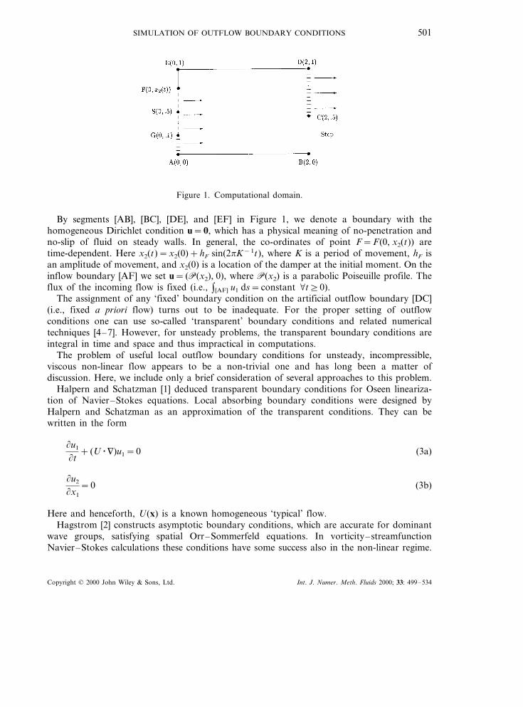
Figure 1. Computational domain.

By segments [AB], [BC], [DE], and [EF] in Figure 1, we denote a boundary with thehomogeneous Dirichlet condition u=0, which has a physical meaning of no-penetration andno-slip of fluid on steady walls. In general, the co-ordinates of point F=F(0, x2(t)) aretime-dependent. Here x2(t)=x2(0)+hF sin(2pK−1t), where K is a period of movement, hF isan amplitude of movement, and x2(0) is a location of the damper at the initial moment. On theinflow boundary [AF] we set u= (P(x2), 0), where P(x2) is a parabolic Poiseuille profile. Theflux of the incoming flow is fixed (i.e., [AF] u1 ds=constant Öt]0).

The assignment of any ‘fixed’ boundary condition on the artificial outflow boundary [DC](i.e., fixed a priori flow) turns out to be inadequate. For the proper setting of outflowconditions one can use so-called ‘transparent’ boundary conditions and related numericaltechniques [4–7]. However, for unsteady problems, the transparent boundary conditions areintegral in time and space and thus impractical in computations.

The problem of useful local outflow boundary conditions for unsteady, incompressible,viscous non-linear flow appears to be a non-trivial one and has long been a matter ofdiscussion. Here, we include only a brief consideration of several approaches to this problem.

Halpern and Schatzman [1] deduced transparent boundary conditions for Oseen lineariza-tion of Navier–Stokes equations. Local absorbing boundary conditions were designed byHalpern and Schatzman as an approximation of the transparent conditions. They can bewritten in the form

(u1

(t+ (U · 9)u1=0 (3a)

(u2

(x1

=0 (3b)

Here and henceforth, U(x) is a known homogeneous ‘typical’ flow.Hagstrom [2] constructs asymptotic boundary conditions, which are accurate for dominant

wave groups, satisfying spatial Orr–Sommerfeld equations. In vorticity–streamfunctionNavier–Stokes calculations these conditions have some success also in the non-linear regime.



Another method, considered by Hagstrom for primitive variables formulation, is the directapplication of the scalings used to approximate spatial Orr–Sommerfeld equations. In terms ofthe physical variables, these are

(

(x1

=O� 1

Re�

,(

(t=O

� 1Re

�Using these scalings it is shown that

(u2

(x1

=O� 1

Re2

�(4a)

p−1

Re(u1

(x1

+C(t)=O� 1

Re2

�(4b)

Here, the function C(t) is an arbitrary constant, which may be added to p. Equations (4a) and(4b) result in boundary conditions after dropping the O(Re−2) terms. Conditions of this typeare quite usual for the Galerkin approach to the Navier–Stokes equations, where appropriateboundary conditions are obtained via specification of a surface traction vector on an artificialboundary. The obtained conditions used to be natural in a weak formulation [8]. For morerecent analyses of such an approach see Bruneau and Fabrie [9] and Heywood et al. [10].

While conditions (4a) and (4b) are satisfied in a finite element formulation, in a weak sensethere direct adaptation for FD methods seems to be questionable. Many (if not most) paperswith an FD approach use (( · )/(n for normal velocity component. In our model problem itcan be the following boundary conditions on [CD]:

(u1

(x1

=0, u2=0 (5a)

or

(u1

(x1

=0,(u2

(x1

=0 (5b)

If we assume function u to be smooth enough, then conditions (5a) guarantee the validationof the equality div u=0 on the artificial boundary. Sometimes, in order to avoid any ‘fixed’conditions on the u2 component, conditions (5b) are used in practice. However, if one wishesvelocity to satisfy conditions (5b), together with the incompressibility equation on theboundary, then the restriction u2=c appears again. Moreover, in the above test problem,c=0. However, for unsteady non-linear flow equations, u2=0 is not the proper choice on anartificial boundary, apparently.

Note also that the loss of the important conjunction property of −div and 9 operators in(5a) and (5b) and the mixed boundary conditions decrease the effectiveness or make it verydifficult to use some numerical methods that are good for solving problems of the Stokes- andNavier–Stokes-type with Dirichlet boundary conditions for the velocity function.



Conditions (3a) and (3b) are more convenient for numerical FD realization, since after theexplicit time discretization of (3a), one has Dirichlet boundary conditions on u · n and so theconjunction property of −div and 9 can be ensured. Although conditions (3a) and (3b) havetheoretical justification in Reference [1] for Navier–Stokes flow, in Section 4 we show thatthey have evident influence upstream on the flow in the non-linear regime. In this case,Equation (3b) seems troublesome. Note that Equation (3b) appears also as (4a) and as (5b). Toavoid this condition for u2 we use the method of scalings and get (u2/(t=O(Re−2), (u2/(x1=O(Re−2). Combining these O(Re−2) terms results in the following boundary condition:

(u2

(t+U1

(u2

(x1

=0 (6)

Unlike (3b), Equation (6) has an unsteady nature and could be more suitable for unsteadyflows. Beside this, Equation (3a) together with Equation (6) provide us with Dirichletconditions u · n and u · t on the outflow boundary after explicit treatment.

In our numerical experiments we formally chose function U through one of the followingways:

(i) U (1)(x)= (Uconstant, 0);(ii) U (2)(x)= (P(x2), 0), where P(x2) is a Poiseuille profile.

Taking into account the proper choice of U (k), Equations (3a) and (6), we can rewrite theoutflow boundary conditions for u in the following way:

(u(t

+U1(k) (u(n

=0, k=1, 2 (7)

In view of rather obvious mechanical interpretation, we call boundary condition (7) the driftconditions, and function U(x) the drift function.

Equations of the transport type were considered on artificial boundaries in various partialdifferential problems. Conditions similar to Equation (7) were introduced for a two-dimensional wave equation [11] (first-order absorbing boundary conditions) and used onartificial boundaries for wave-like equations [12–14].

Looking for analogs in fluid dynamics theory, we should mention non-reflecting boundaryconditions for compressible viscous flow on an artificial boundary [15,16] or their improve-ment for one-dimensional subsonic flows [17]. It was found that non-reflecting conditions aremore effective to reduce a reflection of outflow boundary in contrast to the traditionalconditions for pressure. For a treatment of non-linear problems see Hedstrom [16] andThompson [18]. Ultimately, conditions similar to Equation (7) were mentioned by Gresho [8]as those to be gaining favor (see also Reference [19]). For some other considerations of outflowconditions problem, we also refer to Johanson [20] and Jin and Braza [21].

Let us come back to formula (7). Note that the validity of the equation div u=0 on theartificial boundary together with conditions (7) does not require any ‘fixed conditions onvelocity components u1 or u2. Only for the stationary solution we obtain u2�[CD]=0. In thiscase, conditions (7) coincide with the conditions of Halpern–Schatzman and ‘traditional’ (5b).



Existence and uniqueness theorems for the system of equations (1) and (2), the initial datau0(x), the boundary conditions (7) on [CD], and the Dirichlet conditions on the other part ofboundary hold after time discretization of the system, together with condition (7), i.e., for aknown solution at time t and time step t, functions u(t+t, x) and p(t+t, x) are founduniquely. Note that this is not the case for conditions (5a) and (5b) or for the stationaryproblems when no initial conditions are posed (see the counterexample in Reference [19]). Theextension of these theorems to the differential case requires additional investigations.

For the sake of convenience we will write the ‘fixed’ boundary conditions in the form of (7)taking for them U (0) 0. Then, boundary conditions for u(x, t) will be the same as boundaryconditions for u0(x), where u0(x) is the initial condition at the moment t=0. For u0(x) we takethe solution of the stationary Stokes problem with Poiseuille flow on [AS] and [CD].

It should be noted that for very accurate simulation of the flow phenomena, an artificialboundary should be moved ‘far’ to the right even in the case of absorbing boundary conditionson the outflow. To make the influence of different boundary conditions more clear we do notmove away the outflow boundary in our numerical experiments.

Some further remarks on other absorbing boundary conditions of advection type are givenin Section 5.

3. NUMERICAL SCHEME

To solve Equations (1) and (2) numerically, we use the staggered grid, which proves to be goodenough for the numerical solution of different problems of fluid dynamics [22–25]. Here wedescribe the numerical scheme used. Let V( = [0, 2]× [0, 1], h1=2/N1, h2=1/N2.

Let us introduce the sets

V( 1=!��

i−12�

h1, jh2�

: 05 i5N1+1, 05 j5N2"

V( 2=!�

ih1,�

j−12�

h2�

: 05 i5N1, 05 j5N2+1"

V3=!��

i+12�

h1,�

j+12�

h2�

: 05 i5N1, 05 j5N2"

By H0h we denote a linear space of vector functions defined on V( 1@V( 2 and vanished on the

appropriate grid boundary. Using Lh we denote a space of functions defined on V3, whichsatisfy the condition

%x�V3

ph(x)=0

Operators divh, 9h, (92)h and convective terms N(uh, vh) we define the following [23,25]:



divh u�x�V3= %

2

k=1

hk−1�uk

�x+

hk

2ek

�−uk

�x−

hk

2ek

��, u�H0

h@Hph

{9hph�(x1, x2)�V1@V2}k=hk

−1�ph�xk+hk

2ek

�−ph�xk−

hk

2ek

��, k=1, 2

N1(uh, vh)�x�V1= (4h1)−1[(u1

h(x−h1e1)+u1h(x))(61

h(x)−61h(x−h1e1))

+ (u1h(x)+u1

h(x+h1e1))(61h(x+h1e1)−61

h(x))]+ (4h2)−1

��u2

h�x−(h1e1+h2e2)

2�

+u2h�x+

(h1e1+h2e2)2

��· (61

h(x+h2e2)−61h(x))

+�

u2h�x+

(h1e1−h2e2)2

�+u2

h�x−(h1e1+h2e2)

2��

(612(x)−61

h(x−h2e2))n

N2(uh, vh) is defined similarly. (92)h is the usual five-point approximation of the Laplaceoperator.

Using the notation (aI− (92)h)0−1c, we denote a solution of the equation (aI− (92)h)uh=c,

uh�H0h, where I is the identity operator, a]0 and c is defined in all interior nodes of the grid

domain.Further, we use the notations: u(x)=uh(x, t), u(x)=uh(x, t+t), p(x)=ph(x, t), p(x)=

ph(x, t+t), where t is a time step.We consider the following scheme. If u is known already, then the functions u and p are

determined from

u−ut

=n(92)hu−9hp−N(u, u)

divh u=0, u0=u�t=0

u�G0=0, u�G1

= (Ph(x2), 0)

u(x)=u(u(x)−th1−1U (k)(x)(u(x)−u(x−h1e1))), x�G2 (8)

where G0 is a grid boundary on [AB], [BC], [DE], [EF]; G1 and G2 are grid boundaries on [AF]and [CD] respectively; Ph(x2) is a grid projection of the Poiseuille profile; U (k) (U (k))h is agrid projection of the drift function, k�{0, 1, 2}; u is chosen to satisfy the grid analog of thecondition �(V u · n ds=0.

Note that u=1 in the case of free (without the [BC] step) outlet or for the steady solution,generally u�1+ct2. In the case of k=0, we are solving the problem with ‘fixed’ outflowboundary conditions, and in the case of k=1, 2, we are solving the problem with the driftconditions on the outlet.

For the Halpern–Schatzman boundary conditions, the equation for u2 on G2 in Equations(8) is replaced by



u2(x)− u2(x−h1e1)=0, x�G2

On every time step a problem of the Stokes type with parameters should be solved. Considerthis problem. After transference of Dirichlet non-homogeneous boundary conditions to theright-hand side of the momentum and compressibility equations, and after elimination of ufrom these equations, we can rewrite the problem in the following way:

divh((nt)−1I− (92)h)0−19hp= f h (9)

Equation (9) is effectively solved by the conjugate gradient method with the preconditioner[26].

No additional calculations are needed to recover the velocity field u. Moreover, u exactlysatisfies the incompressibility condition for the accurate solution of (9).

4. NUMERICAL RESULTS

In this section we present and compare results of calculations carried out for the followingproblems with different outflow conditions (see Figure 1):

(I) The damper [EF] moves up and down with a period of 0.5; the extreme positions of pointF are (0, 0.9) and (0, 0.1); x2(0)=0.5; [AF(t)] u1 ds=1, Öt]0; all the interval [BD] isconsidered as the outflow boundary (i.e., point C coincides with B).

(II) The inflow conditions are the same as in the problem I, except on the outlet [BC] the stepof height 0.5 is disposed of.

For both problems we also compute a so-called ‘exact’ solution. For problem I, this is asolution calculated with the outflow boundary moved far to the right (V( = [0, 16]× [0, 1], andfor problem II this is a solution of the real forward-facing step problem with the step lengthof 6.

There are a large number of ways to define the Reynolds number Re=Vl/n. For theproblems considered it was naturally to choose

V=maxt]0

��AF(t)�−1&[AF]

u1 ds�

l=1 is the channel height, n is the kinematic viscosity. Thus, we have Re=10n−1.

4.1. On stability of numerical schemes

Using numerical scheme (8) for calculations, one has to keep in mind the conditional stabilityof this scheme. Restrictions on the time step appear owing to an approximation of theconvective terms on the previous time layer. For the sufficient stability conditions of (8) withDirichlet boundary conditions see Reference [27].



At the same time the discrete analog of drift boundary conditions, which we used (Section3), can be considered as an approximation of the one-dimensional transfer equation by anexplicit, conditionally stable scheme.

Thus, one may expect that the drift boundary conditions could prevent the further loss ofstability of the numerical scheme. That is why we turn our attention now to the checking ofthe stability of numerical scheme (8) for U (1) and U (2).

Numerical experiments were carried out for the problem I. The test below was used toinvestigate the stability of scheme (8). The numerical scheme was said to be stable if thefollowing relation was valid:

maxt� [0,t 1]

u(t) u(0) 5M

where t1=10K, M=100, �� · �� is the L2 norm.In Table I one can see values of maximum t, for which numerical scheme (8) is stable in the

above sense.The values of t from Table I were found through the dichotomy method for solving the

problem x(t)=0.5 with the aspect error 0.001, where

x(t)=�0, if the problem is not stable

1, if the problem is stable

Symbol * in Table I means that for different initial values of t, the calculated results differand lie in the interval [0.00014, 0.00025]. This effect indicates irregular behavior of the functionx near the point of stability loss for numerical scheme with U (0), n=5×10−4.

We can see from Table I that restrictions on the time step, which we have to introduce toguarantee stability, are not stronger for the drift conditions U (1) and U (2) than for ‘fixed’boundary conditions (U (0)), and they are slightly weaker for higher Re.

The above criterion does not guarantee that exponential instability is suppressed for all t

calculated. This criterion is used only for comparison. However, the calculated values of t arevery close to critical. In Figure 2 we show the evolution of the solution through time with

Table I. Critical t for stability of scheme grid 32×64, Re=10n−1, t1=5.

U2U1U0n¯U

0.03 0.00631 0.00631 0.006310.001000.01 0.00100 0.00100

0.000263 0.000293 0.0002690.001* 0.000148 0.0001240.0005



Figure 2. Behavior of velocity spatial norms for t=0.001 and t=0.00105.

n=0.01, U2, t=0.00105 and t=0.001. For t=0.00105 the solution blows up and fort=0.001 calculations are stable. The solutions of the problem for t=0.001 and for t=5×10−4 that guarantee stability of the scheme were in a very good agreement.

4.2. On accuracy of numerical schemes

While results on accuracy of the marker and cell (MAC) scheme are well known (seeReference [28]) and the use of this scheme in computational fluid dynamics has a longhistory, its application with given data requires additional checking of convergence. Tothis end, the ‘exact’ solution of problem I was calculated on four embedded grids,with h=1/16, 1/32, 1/64, and 1/128 respectively, and other data fixed, in particular n=0.01.Pointwise convergence was detected both for pressure and velocity; see Figure 3 as anillustration for two points. Solutions for h=1/64 and h=1/128 practically coincide. Aminor loss of convergence in pressure is due to the well-known lack of regularity for pressurefunction in comparison with velocity. The grid with h=1/64 was chosen for our furthercalculations.

4.3. General form of solution, influence of boundary conditions

Calculations were performed with n=0.01 (Re=103), and the time interval equal to 20K,where K=0.5 is the period of damper movement. Setting t=2×10−4 to reach the stabilityof the numerical scheme (Table I), we obtain solutions of the problem with the drift boundary



Figure 3. Time histories of u1, u2 and p in point (1, 0.5) and p in (2, 0.875), where – +× –, h=1/16; – – –,h=1/32; —, h=1/64; – –, h=1/128.

conditions (U (k), k=0, 1, 2), Halpern–Schatzman (HS) boundary conditions, and the ‘exact’solution on time interval [0, 20K ]. A solution of the stationary Stokes problem was consideredas the initial value; therefore, the further evolution of the flow can be divided into twoqualitatively different stages



(I) the stage of periodic solution formation(II) the stage of periodic behavior of the solution

The duration of the first stage can be estimated approximately as 4K (or �2). For theoutflow boundary without the [BC] step, the typical behavior of the flow is demonstrated inFigures 4–8 (we show streamlines for not-time-average data).

At first the single vortex is formed behind the damper. Since the damper goes down and theaverage inflow velocity increases, the intensity of the vortex is growing and its center is movingdown.

Sufficiently large Reynolds number and small period K provide separation of this vortexwhen the damper goes up; after separation, the vortex drifts downstream. Here, the generalform of solutions for all considered problems is the same (Figure 4).

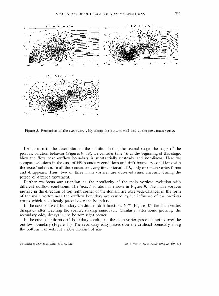
On time interval from 0.5 up to 1.0, the form of solutions for different boundary conditionsis also practically the same and is shown in Figure 5. Here, as well as on every period ofdamper movement, the large vortex is forming behind the damper with its further progressdownstream. These large vortices are said to be ‘main’.

Along the bottom wall, the bending streamlines form a new smaller eddy, recirculating in theopposite direction as that within the main vortex. Further, the formation and downstreamprogress of the smaller secondary eddy along the bottom wall happen at every period ofdamper movement. Formation of these downstream moving eddies for the transitional andturbulent regimes in a channel with a backwards-facing step is reported in Reference [29].

Beginning with time 2K, differences in the flow behavior for various boundary conditionsbecome appreciable (Figures 6–8). Most of all, differences in the behavior of the secondaryeddy along the bottom wall are noted. Thus, in the case of ‘fixed’ boundary conditions (Figure6), the eddy decays after reaching the artificial boundary; in the case of uniform driftconditions (drift conditions with U (1)) (Figure 7), the eddy passes over the artificial boundaryunnaturally increasing; finally, in the case of Poiseuille drift conditions (with U (2)) (Figure 8),the eddy also passes over the boundary with a less increase. In the latter case, the solutioncoincides with the ‘exact’ one.

Figure 4. The main vortex is forming and moving downstream.



Figure 5. Formation of the secondary eddy along the bottom wall and of the next main vortex.

Let us turn to the description of the solution during the second stage, the stage of theperiodic solution behavior (Figures 9–13); we consider time 4K as the beginning of this stage.Now the flow near outflow boundary is substantially unsteady and non-linear. Here wecompare solutions in the case of HS boundary conditions and drift boundary conditions withthe ‘exact’ solution. In all these cases, on every time interval of K, only one main vortex formsand disappears. Thus, two or three main vortices are observed simultaneously during theperiod of damper movement.

Further we focus our attention on the peculiarity of the main vortices evolution withdifferent outflow conditions. The ‘exact’ solution is shown in Figure 9. The main vorticesmoving in the direction of top right corner of the domain are observed. Changes in the formof the main vortex near the outflow boundary are caused by the influence of the previousvortex which has already passed over the boundary.

In the case of ‘fixed’ boundary conditions (drift function: U (0)) (Figure 10), the main vortexdissipates after reaching the corner, staying immovable. Similarly, after some growing, thesecondary eddy decays in the bottom right corner.

In the case of uniform drift boundary conditions, the main vortex passes smoothly over theoutflow boundary (Figure 11). The secondary eddy passes over the artificial boundary alongthe bottom wall without visible changes of size.



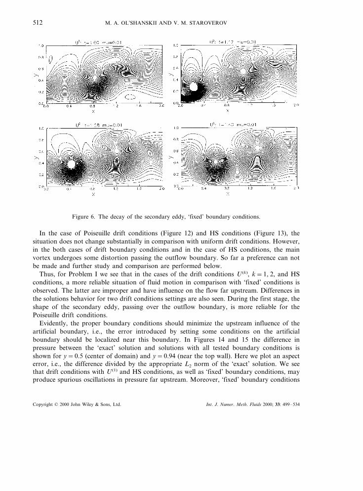
Figure 6. The decay of the secondary eddy, ‘fixed’ boundary conditions.

In the case of Poiseuille drift conditions (Figure 12) and HS conditions (Figure 13), thesituation does not change substantially in comparison with uniform drift conditions. However,in the both cases of drift boundary conditions and in the case of HS conditions, the mainvortex undergoes some distortion passing the outflow boundary. So far a preference can notbe made and further study and comparison are performed below.

Thus, for Problem I we see that in the cases of the drift conditions U (k), k=1, 2, and HSconditions, a more reliable situation of fluid motion in comparison with ‘fixed’ conditions isobserved. The latter are improper and have influence on the flow far upstream. Differences inthe solutions behavior for two drift conditions settings are also seen. During the first stage, theshape of the secondary eddy, passing over the outflow boundary, is more reliable for thePoiseuille drift conditions.

Evidently, the proper boundary conditions should minimize the upstream influence of theartificial boundary, i.e., the error introduced by setting some conditions on the artificialboundary should be localized near this boundary. In Figures 14 and 15 the difference inpressure between the ‘exact’ solution and solutions with all tested boundary conditions isshown for y=0.5 (center of domain) and y=0.94 (near the top wall). Here we plot an aspecterror, i.e., the difference divided by the appropriate L2 norm of the ‘exact’ solution. We seethat drift conditions with U (1) and HS conditions, as well as ‘fixed’ boundary conditions, mayproduce spurious oscillations in pressure far upstream. Moreover, ‘fixed’ boundary conditions



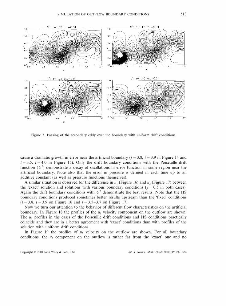
Figure 7. Passing of the secondary eddy over the boundary with uniform drift conditions.

cause a dramatic growth in error near the artificial boundary (t=3.8, t=3.9 in Figure 14 andt=3.5, t=4.0 in Figure 15). Only the drift boundary conditions with the Poiseuille driftfunction (U2) demonstrate a decay of oscillations in error function in some region near theartificial boundary. Note also that the error in pressure is defined in each time up to anadditive constant (as well as pressure functions themselves).

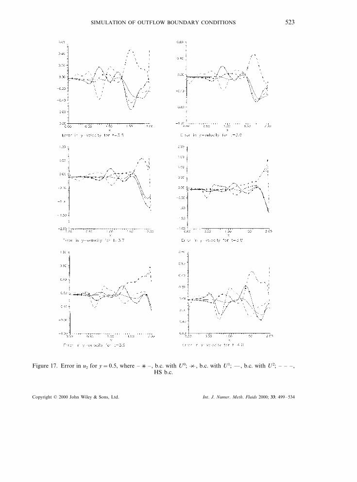
A similar situation is observed for the difference in u1 (Figure 16) and u2 (Figure 17) betweenthe ‘exact’ solution and solutions with various boundary conditions (y=0.5 in both cases).Again the drift boundary conditions with U2 demonstrate the best results. Note that the HSboundary conditions produced sometimes better results upstream than the ‘fixed’ conditions(t=3.8, t=3.9 on Figure 16 and t=3.5–3.7 on Figure 17).

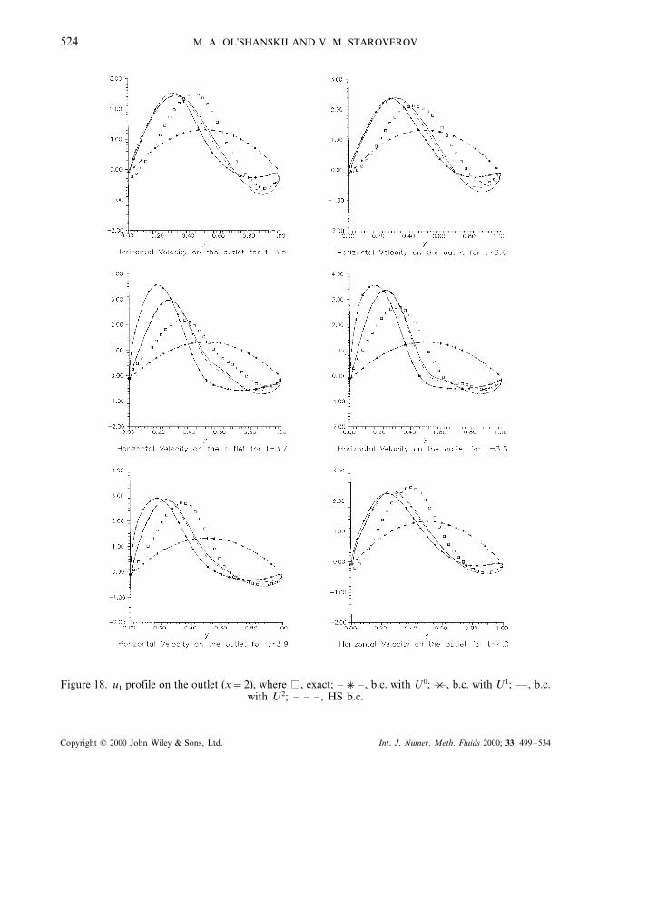
Now we turn our attention to the behavior of different flow characteristics on the artificialboundary. In Figure 18 the profiles of the u1 velocity component on the outflow are shown.The u1 profiles in the cases of the Poiseuille drift conditions and HS conditions practicallycoincide and they are in a better agreement with ‘exact’ conditions than with profiles of thesolution with uniform drift conditions.

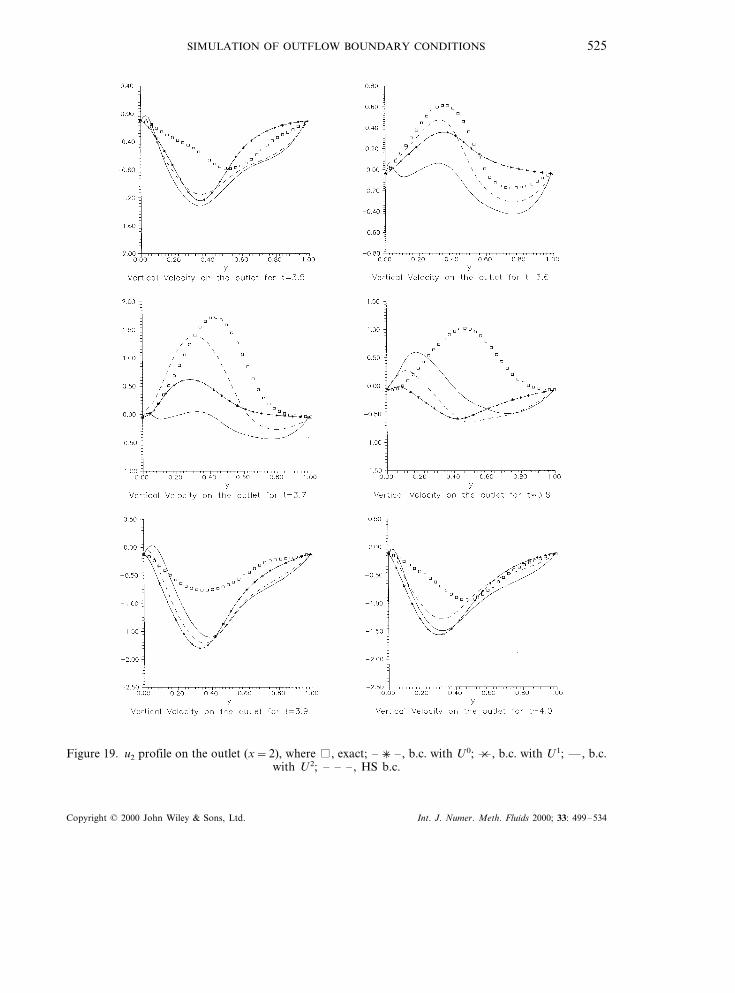
In Figure 19 the profiles of u2 velocity on the outflow are shown. For all boundaryconditions, the u2 component on the outflow is rather far from the ‘exact’ one and no



Figure 8. Passing of the secondary eddy over the boundary with Poiseuille drift conditions.

preference could be given. It seems that the observation of velocity profiles on the artificialboundary helps us to explain the success of the Poiseuille drift conditions in comparison withuniform drift conditions, but not yet with HS conditions. This is why we also compare thenormal derivatives of velocity components on the outflow.

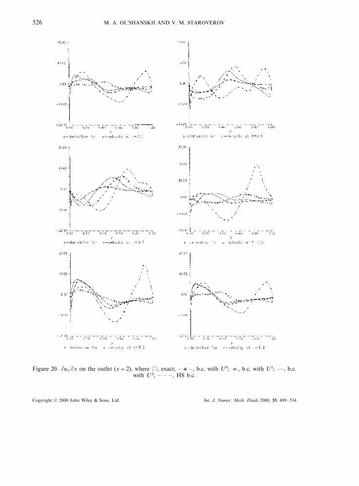
In Figure 20 we show (u1/(n on the outflow. For the Poiseuille drift conditions and HSconditions, the results are the same and only qualitatively correspond to the ‘exact’ derivativesfor some t.

In Figure 21 we show (u2/(n on the outflow. We recall that (u2/(n=0 for HS conditions,and from Figure 21, we see that this condition is too far from being satisfied by the ‘exact’solution. It seems that the drift boundary conditions with U2 and even with U1 produce abetter approximation of (u2/(n on the outflow than HS conditions. We propose that thesuccess of the Poiseuille drift conditions is due to the better approximation of the normalderivative of u2 in comparison with (u2/(n=0. For the ‘fixed’ boundary conditions, the valuesof (u1/(n and (u2/(n are absolutely wrong.

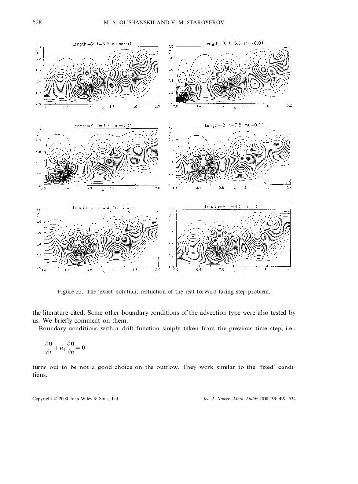
Now we will present some results for Problem II. In Figures 22–25 we show the full periodof problem II solutions (i.e., with the [BC] step on the outflow), the exact one (Figure 22) andwith various boundary conditions.



Figure 9. The ‘exact’ solution; restriction of the elongated computational domain.

As well as in Problem I, we carried out our calculations on time interval [0, 20K ]with t=2×10−4, n=0.01. After 4K, solutions have a periodic behavior. Now the second-ary eddy, moving along the bottom wall, does not approach the outflow boundary,but flowing together with the small eddy at the base of the [BC] step, leads to its pul-sation.

For the ‘fixed’ boundary conditions (Figure 23), just as in Problem I, a gradual decay of themain vortex is observed in the top right corner of the domain.



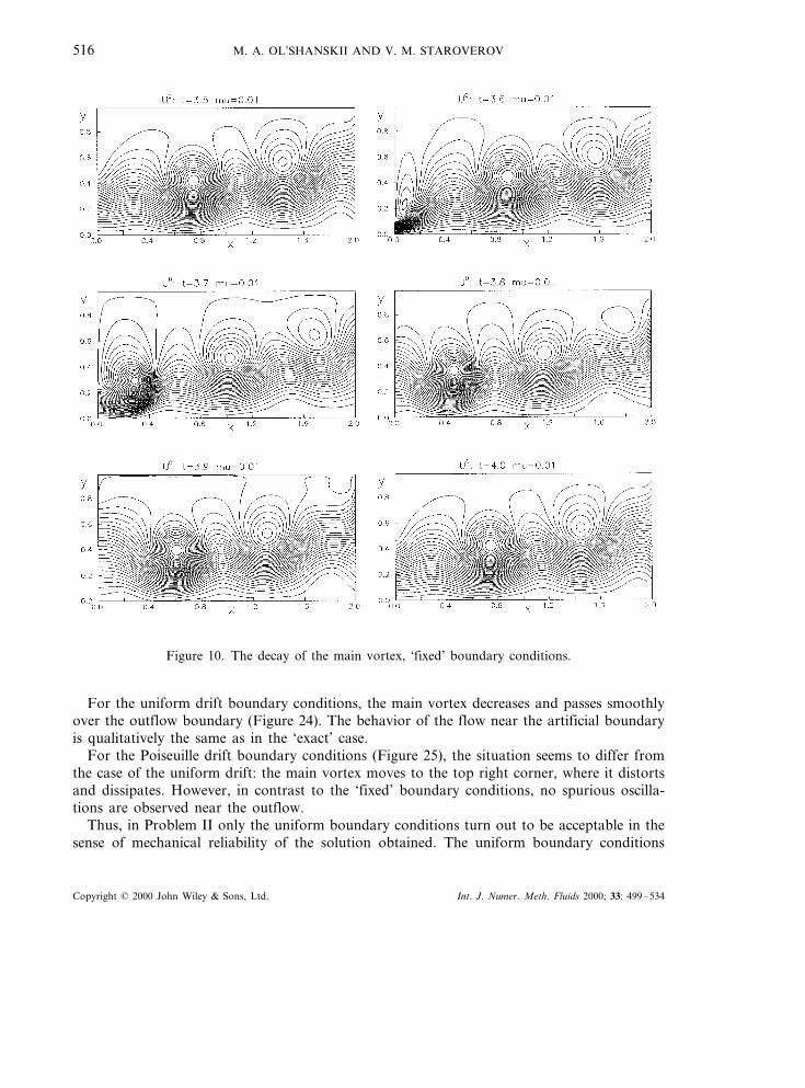
Figure 10. The decay of the main vortex, ‘fixed’ boundary conditions.

For the uniform drift boundary conditions, the main vortex decreases and passes smoothlyover the outflow boundary (Figure 24). The behavior of the flow near the artificial boundaryis qualitatively the same as in the ‘exact’ case.

For the Poiseuille drift boundary conditions (Figure 25), the situation seems to differ fromthe case of the uniform drift: the main vortex moves to the top right corner, where it distortsand dissipates. However, in contrast to the ‘fixed’ boundary conditions, no spurious oscilla-tions are observed near the outflow.

Thus, in Problem II only the uniform boundary conditions turn out to be acceptable in thesense of mechanical reliability of the solution obtained. The uniform boundary conditions



Figure 11. Passing of the main eddy over the boundary with uniform drift conditions.

appear probably to be the most preferable, when a ‘typical’ flow U (see Section 2) cannot bedistinguished on the outflow boundary.

In Figure 26 we demonstrate the difference in pressure between the ‘exact’ solution andsolutions with the drift boundary conditions Uk, k=0, 1, 2 for y=0.75. All boundaryconditions have approximately the same upstream influence.

4.4. On computational inputs

To give a quantitative idea of the computational inputs we present in Table II the CPU timeneeded for some problems considered.



Figure 12. Passing of the main eddy over the boundary with Poiseuille drift conditions.

Almost the same CPU time for the problems with various boundary conditions (otherparameters are fixed) indicates that norms of solution differences on neighboring time layershave approximately the same ratio and the cost of one time step was the same for allconsidered boundary conditions.

Note that the 2.5-times increase in the number of time steps and 2-times increase in thenumber of grid points provided only a 2.4-times increase in CPU time. It can be explained,firstly, by the 2-times reduction in norms of solutions’ differences on neighboring time layers



Figure 13. Passing of the main eddy over the boundary with HS boundary conditions.

and, secondly, decreasing of t (as well as n) implies growth of convergence rate of the interioriterative process used (see Section 3 and Reference [26]).

5. REMARKS AND CONCLUSIONS

Much more various combinations of velocity components and their derivatives can beconsidered on the artificial boundary as an outflow condition. Many of them can be found in



Figure 14. Error in pressure for y=0.5, where – +× –, b.c. with U0; —*× , b.c. with U1; —, b.c. with U2;– – –, HS b.c.



Figure 15. Error in pressure for y=0.94, where – +× –, b.c. with U0; —*× , b.c. with U1; —, b.c. with U2;– – –, HS b.c.



Figure 16. Error in u1 for y=0.5, – +× –, b.c. with U0; —*× , b.c. with U1; —, b.c. with U2; – – –, HSb.c.



Figure 17. Error in u2 for y=0.5, where – +× –, b.c. with U0; —*× , b.c. with U1; —, b.c. with U2; – – –,HS b.c.



Figure 18. u1 profile on the outlet (x=2), where , exact; – +× –, b.c. with U0; —*× , b.c. with U1; —, b.c.with U2; – – –, HS b.c.



Figure 19. u2 profile on the outlet (x=2), where , exact; – +× –, b.c. with U0; —*× , b.c. with U1; —, b.c.with U2; – – –, HS b.c.



Figure 20. (u1/(x on the outlet (x=2), where , exact; – +× –, b.c. with U0; —*× , b.c. with U1; —, b.c.with U2; – – –, HS b.c.



Figure 21. (u2/(x on the outlet (x=2), where , exact; – +× –, b.c. with U0; —*× , b.c. with U1; —, b.c.with U2; – – –, HS b.c.



Figure 22. The ‘exact’ solution; restriction of the real forward-facing step problem.

the literature cited. Some other boundary conditions of the advection type were also tested byus. We briefly comment on them.

Boundary conditions with a drift function simply taken from the previous time step, i.e.,

(u(t

+u1

(u(n

=0

turns out to be not a good choice on the outflow. They work similar to the ‘fixed’ condi-tions.



Figure 23. The decay of the main vortex with ‘fixed’ boundary conditions, [BC] step is on the outlet.

The following boundary conditions:

(u1

(t+U1

(k) (u1

(n=0, k=1, 2

u2=0

were also tested and showed themselves to be of the absorbing type. The behavior of the flowwas rather like in the case of uniform drift outflow conditions.



Figure 24. Passing of the main eddy over the boundary with uniform drift conditions, [BC] step is on theoutlet.

Resuming the results of all experiments we state that the drift boundary conditions withappropriate drift function is the best choice in the considered class of absorbing outflowconditions. They really suppress an upstream influence of the artificial boundary and at thesame time they are convenient in computations via various finite methods. When there is noappropriate drift function, the uniform drift conditions seems to be the proper choice.Anyway, the good choice of the drift function in (7) is quite important.

Finally, we propose that a good approximation of u1, (u1/(n, and (u2/(n on the artificialboundary is of major importance, while the approximation of u2 is of minor one.



Figure 25. The decay of the main vortex with Poiseuille drift boundary conditions, [BC] step is on theoutlet.

Table II. Computing time for RISC-6000 processor (h:min); n=0.01, Re=103, t1=5.

t N×M U0Outlet U1 U2

5×10−4 32×64Free 5:44 5:39 5:395:41 5:40 5:40

2×10−4 64×64 13:23[BC] step 13:25 13:32



Figure 26. Error in pressure for y=0.75, where – +× –, b.c. with U0; —*× , b.c. with U1; —, b.c. with U2.



ACKNOWLEDGMENTS

The authors would like to thank E.V. Chizhonkov, G.M. Kobelkov, and A.G. Sokolov for helpfuldiscussions and many useful comments. The work was performed with computer support of theFrench–Russian A.M. Liapunov Institute of Applied Mathematics and Informatics and was supportedin part by RFFI grant 96-01-01254 and by INTAS grant 93-0377-EXT for both authors.

REFERENCES

1. Halpern L, Schatzman M. Artificial boundary conditions for incompressible viscous flows. SIAM Journal ofMathematics and Analysis 1989; 20: 308–353.

2. Hagstrom T. Conditions at the downstream boundary for simulations of viscous, incompressible flow. SIAMJournal of Science, Statistics and Computers 1991; 12: 843–858.

3. Landau LD, Lifshits EM. Fluid Mechanics. Pergamon: New York, 1975.4. Ferm L, Gunstafsson B. A downstream boundary procedure for the Euler equations. Computers and Fluids 1982;

10: 261–276.5. Johnson C, Nedelec JC. On the coupling of boundary integral and the finite element methods. Mathematics and

Computers 1980; 35: 1063–1079.6. Lenoir M, Tounsi A. The localized finite element method and its application to the 2D seakeeping problem. SIAM

Journal of Numerical Analysis 1988; 25: 729–752.7. Sequeira A. The coupling of boundary integral and finite element methods for the bidimentional steady Stokes

problem. Mathematical Methods and Applications in Science 1983; 5: 356–376.8. Gresho PM. Incompressible fluid dynamics: some fundamental formulation issues. Annual Re6iews in Fluid

Mechanics 1991; 23: 413–453.9. Bruneau ChH, Fabrie P. Effective downstream boundary conditions for incompressible Navier–Stokes equations.

International Journal for Numerical Methods in Fluids 1994; 19: 693–705.10. Heywood JG, Rannacher R, Turek S. Artificial boundaries and flux and pressure conditions for the incompress-

ible Navier–Stokes equations. International Journal for Numerical Methods in Fluids 1996; 22: 325–352.11. Engquist B, Majda A. Absorbing boundary conditions for numerical simulations of waves. Mathematics and

Computers 1977; 31: 629–651.12. Bayliss A, Turkel E. Radiation boundary conditions for wave-like equations. Communications in Pure and Applied

Mathematics 1980; 33: 707–725.13. Clayton R, Engquist B. Absorbing boundary conditions for acoustic and elastic wave equations. Bulletin of the

Seismology Society of America 1977; 67: 1529–1540.14. Engquist B, Majda A. Radiational boundary conditions for acoustic and elastic wave calculations. Communica-

tions in Pure and Applied Mathematics 1979; 32: 313–357.15. Bayliss A, Turkel E. Far field boundary conditions for compressible flow. Journal of Computational Physics 1982;

48: 182–199.16. Hedstrom GW. Non-reflecting boundary conditions for nonlinear hyperbolic systems. Journal of Computational

Physics 1979; 30: 222–237.17. Rudy DH, Strikwerda JC. A nonreflecting outflow boundary conditions for subsonic Navier–Stokes calculations.

Journal of Computational Physics 1980; 36: 55–70.18. Thompson KW. Time dependent boundary conditions for hyperbolic systems. Journal of Computational Physics

1987; 68: 1–24.19. Sani RL, Gresho PM. Resume and remarks on the open boundary condition minisymposium. International

Journal for Numerical Methods in Fluids 1994; 18: 983–1008.20. Johansson V. Boundary conditions for open boundaries for the incompressible Navier–Stokes equations. Journal

of Computational Physics 1993; 105: 233–251.21. Jin G, Braza M. A nonreflecting outlet boundary condition for incompressible unsteady Navier–Stokes calcula-

tions. Journal of Computational Physics 1993; 107: 239–253.22. Gustafson K, Halasi K. Vortex dynamics of cavity flows. Journal of Computational Physics 1986; 64: 279–319.23. Kobelkov GM. On numerical methods of solving the Navier–Stokes equations in ‘velocity-pressure’ variables. In

Numerical Methods and Applications, Marchuk C (ed.). CRC Press: New York, 1994; 81–115.24. Kobelkov GM. Solution of stationary free convection problem. Doklady Academii Nauk SSSR 1980; 255:

277–282.25. Fletcher CAJ. Computational Techniques for Fluid Dynamics 2. Springer: New York, 1988.



26. Ol’shanskii MA. On the numerical solution of the nonstationary Stokes equations. Russian Journal of NumericalAnalysis and Mathematical Modelling 1995; 10: 81–92.

27. Temam P. Na6ier–Stokes Equations. Theory and Numerical Analysis. North Holland: Amsterdam, 1979.28. Nicolaides RA. Analysis and covergence of the MAC scheme I. The linear problem. SIAM Journal of Numerical

Analysis 1992; 29: 1579–1591.29. Armaly BF, Durst F, Pereira JCF, Schonung B. Experimental and theoretical investigation of backward-facing

step flow. Journal of Fluid Mechanics 1983; 127: 473–496.


on simulation of outflow boundary conditions in finite ...molshan/ftp/pub/outflow.pdf · on...

Documents