industrial engineering college of engineering bayesian kernel methods for binary classification and...
TRANSCRIPT

Industrial EngineeringCollege of Engineering
Bayesian Kernel Methods for Binary Classification and Online Learning Problems
Theodore TrafalisWorkshop on Clustering and Search Techniques in Large Scale Networks
LATNA, Nizhny Novgorod, Russia, November 4, 2014

Part I.Bayesian Kernel Methodsfor Gaussian Processes

Why Bayesian Learning?
•Returns a probability
• Incorporates power of kernel methods with advantages of Bayesian updating
•Can incorporate prior knowledge into estimation
•Can “learn” fairly quickly if Gaussian process
•Can be used for regression or classification
Outline
1. Bayesics
2. Relevance Vector Machine
3. Laplace Approximation
4. Results

Bayes’ Rule
)(
||,|
yxtxty
yxtxytP
PPPP
xtxtyyxt PPP ||
Calculated value Posterior PriorLikelihood

Logistic Likelihood
i
iii xt
xtxtyP
exp1exp
1|
ixt
exp11

Prior
•Assume t(x) = {t(x1), …, t(xm)} is a Gaussian process (normally distributed)
• Let t = Kα
mxtxt ,..., cov 1K
αKαKα T21
21
exp det2
1m
P
m
jjjii xxKxt
1
),(
xt0 E

Maximize Posterior
xtxtyyxt PPP ||
ααyyα PPP ||
ααyα PyPPm
ii
1
||
Goal: Find optimal values for α

Minimize Negative Log
ααyα PyPPm
ii log|log|log
1
1,exp1,exp1log|log ii yi
yii xKxKyP αxαxα
αxαx ,exp1log1,exp1log iiii xKyxKy
= 1 if yi = 0 = 1 if yi = 1
m
jjji
iii
xxKxt
xtyP
1
,exp1
1exp1
11|

Minimize Negative Log
ααyα PyPPm
ii log|log|log
1
αKαKα T21
21
exp det2
1n
P
αKαα T
21
log P
Kααα T
1 21
|logmin
m
iiyP

Relevance Vector Machine
•Combines Bayesian approach with sparseness of support vector machine
•Previously
•Hyperparameter
αKαKα T21
21
exp det2
1m
P
2
21
exp2
| iii
ii αss
sαP
αSαSsα T21
21
exp2
1|
mP
1/Variance(αi)

Non-Informative (Flat) Prior
baGammasP i ,~
Let a = b ≈ 0

Maximize Posterior
m
iii
m
ii PsPyPP
11
log|log|log,|log sαsyα

Laplace ApproximationNewton-Raphson Method
zfzf
zz
oldnew
αx
αxαxαx
xαα ,exp1,exp1
,exp1,exp
,|logi
ii
i
iiii xK
xKyxKxKy
xKyP
x
αxαx
αxαx
xαα ,,exp1
,exp1,exp1,exp
,|log 22T2
ii
ii
i
iiii xK
xKxKy
xKxKy
xKyP
αSα
m
iii sP
1
|log
ci
Cii

Iteration
old1T
oldnew αSKcSCKKαα

Optimizing Hyperparameter
•Need a closed-form expression for
• If α|y,s were normally distributed, then at optimal
•Use Gaussian approximation
ys|P
2
2 ,|log1
i
iiii E
Pss
syαα
2
1T1
i
ii
ss
i i
SCKK

SVM and RVM Comparison
Classification Data Set m d SVM RVM SVM RVMPima Diabetes 200 8 20.1% 19.6% 109 4U.S.P.S. 7291 256 4.4% 5.1% 2540 316Banana 400 2 10.9% 10.8% 135.2 11.4Breast Cancer 200 9 26.9% 29.9% 116.7 6.3Titanic 150 3 22.1% 23.0% 93.7 65.3Waveform 400 21 10.3% 10.9% 146.4 14.6German 700 20 22.6% 22.2% 411.2 12.5Image 1300 18 3.0% 3.9% 166.6 34.6Normalized Mean 1 1.08 1 0.17
errors vectors
Similar accuracy with fewer “support” vectors

Conclusion
•Posterior Likelihood x Prior
•Gaussian process ▫Makes math easier▫Assumes that density is centered around mode
•Relevance Vector Machine ▫Similar accuracy to Support Vector Machine ▫Fewer data points for RVM compared to SVM
• In part 2 we discuss▫Non-Gaussian process▫Markov Chain Monte Carlo solution

References
•B. Schӧlkopf and A.J. Smola, 2002. “Chapter 16: Bayesian Kernel Methods.” Learning With Kernels: Support Vector Machines, Regularization, Optimization, and Beyond. Cambridge: MIT Press.
•C.M. Bishop and M.E. Tipping, 2003. “Bayesian Regression and Classification.” In J. Suykens, G. Horvath, S. Basu, C. Micchelli, and J. Vandewalle, eds. Advances in Learning Theory: Methods Models and Applications. Amsterdam: IOS Press.

Backup

Likelihood for Classification
• Logistic
•Probit
i
iii xf
xfxfyP
exp1exp
1|
iii xfy sgn
,N~i 0
ii
xfyii
xfydxfyP
ii
2
2
2 2exp
2
1sgn

Likelihood for Regression
iii xty
iiiii PxtyPxtyP |

RVM for Regression
μαΣμαΣα 1T212
21
exp2
1,,| -
nP
sy
where
1T2 SKKΣ
KyΣμ 2

Incremental Updating for Regression
2
oldnew 1
i
iiii
ss
n
iii
oldi
new
s
Ky
1
22

Industrial EngineeringCollege of Engineering
Part II. Bayesian Kernel MethodsUsing Beta Distributions
Theodore TrafalisWorkshop on Clustering and Search Techniques in Large Scale Networks
LATNA, Nizhny Novgorod, Russia, November 4, 2014
Summary of Part 1
•Bayesian method: Posterior Likelihood x Prior
•Gaussian process ▫Makes math easier▫Assumes that density is centered around mode
•Relevance Vector Machine
•Solution concept: posterior maximization

Current Bayesian Kernel methods•Combine Bayesian probability with Kernel Methods
•n data points, m attributes per data point
•X is n x m matrix
•y is n x 1 vector of 0s and 1s
•q(X) is a function of X used to predict y
)(
||
yXXy
yXP
PPP
Posterior PriorLikelihood

28MacKenzie and Trafalis
Support Vector Machines

What’s new in part 2
•Beta distributions as priors
•Adaptation of beta-binomial updating formula
•Comparison of beta kernel classifiers with existing SVM classifiers
•Online learning

Outline
1. Beta Distribution
2. Other Priors
3. Markov Chain Monte Carlo
4. Test Case

Likelihood
• Logistic Likelihood
•Bernoulli Likelihood
iii xt
xtyP
exp1
11|
iiyP 1

Beta Distribution Prior
iii Beta ,~
ii
iiE
33MacKenzie and Trafalis
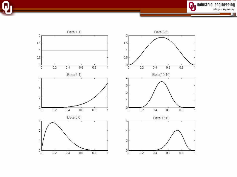
Shape of beta distribution
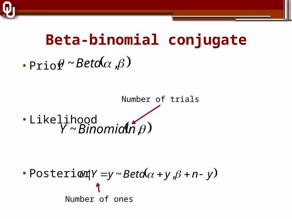
Beta-binomial conjugate
•Prior
• Likelihood
•Posterior
,~ Beta
,~ nBinomialY
ynyBetayY ,~|
Number of ones
Number of trials
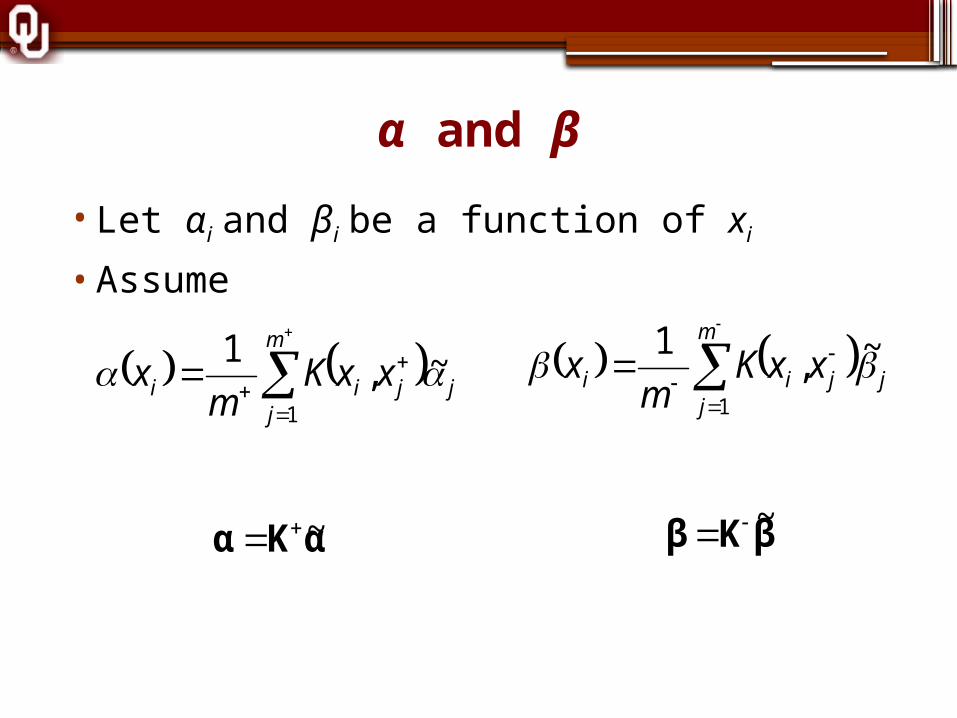
α and β
• Let αi and βi be a function of xi
•Assume
m
jjjii xxK
mx
1
~,1
m
jjjii xxK
mx
1
~,1
αKα ~ βKβ ~

α and β
• Let αi and βi be a function of xi
•Assume
m
jjjii xxK
mx
1
~,1
m
jjjii xxK
mx
1
~,1
αKα ~ βKβ ~

α and β
• Let αi and βi be a function of xi
•Assume
m
jjjii xxK
mx
1
~,1
m
jjjii xxK
mx
1
~,1
αKα ~ βKβ ~

α and β
• Let αi and βi be a function of xi
•Assume
m
jjjii xxK
mx
1
~,1
m
jjjii xxK
mx
1
~,1
αKα ~ βKβ ~

Applying beta-binomial to data mining
•Prior
•Posterior
iii Beta ,~x
01
,1 ,,~|jj y
ijiy
ijii KKBeta xxxxyx
nn
2
2
2
2exp,
ij
ijKxx
xx
Number of zeros in training set
Parameter to be tuned

Classification Rule
• The most likely estimate is the expected value of the beta posterior distribution
• Proposition: The following classification rules are equivalent.
1. Given a uniform prior where α=1 and β=1 and the weights as depicted above, an unknown point should be positively classified if and negatively classified if
2. Given a nonuniform prior where = and if weights are not deployed to update θ an unknown point y should be positively classified if and negatively else.

41MacKenzie and Trafalis
Testing on data sets
Beta prior is uniform: a = 1, b = 1Rates represent mean values of percent of ones or zeros correctly classified
Data setPercentage of ones in data set
Beta priorWeighted
SVMRegular
SVM
TP rate 86 91 98TN rate 95 76 75TP rate 80 87 59TN rate 97 91 99TP rate 87 78 77TN rate 85 93 95TP rate 85 85 85TN rate 85 93 95TP rate 71 69 24TN rate 61 64 94
Parkinson
Tornado
Colon Cancer
Spam
Transfusion
75%
7%
35%
39%
24%

42MacKenzie and Trafalis
Online learning
E[ ] E[ ] E[ ]Prior 1 1 1 0.7 9.3 0.07 0.7 9.3 0.07
1 1.01 1.00 0.50 0.71 9.30 0.07 0.71 9.30 0.072 1.01 1.00 0.50 0.71 9.30 0.07 0.71 9.30 0.073 1.10 1.00 0.52 0.80 9.30 0.08 0.81 9.30 0.085 1.16 1.00 0.54 0.86 9.30 0.08 0.88 9.38 0.09
10 1.49 1.01 0.60 1.19 9.31 0.11 1.22 9.41 0.11
Weighted likelihood Weighted likelihood Unweighted likelihoodTrial
E[ ] E[ ] E[ ]Prior 1 1 1 0.7 9.3 0.07 0.7 9.3 0.07
1 1.00 1.13 0.47 0.70 9.43 0.07 0.70 16.03 0.042 1.02 1.42 0.42 0.72 9.72 0.07 0.72 21.82 0.033 1.02 1.93 0.35 0.72 10.23 0.07 0.72 27.47 0.035 1.08 2.41 0.31 0.78 10.71 0.07 0.78 38.13 0.02
10 1.24 3.95 0.24 0.94 12.25 0.07 0.95 66.24 0.01
Weighted likelihood Weighted likelihood Unweighted likelihoodTrial
Updated probabilities for one data point from tornado data
y = 0
y = 1
Each trial uses 100 data points to update prior

Conclusions
•Adapting the beta-binomial updating rule to a kernel-based classifier can create a fast and accurate data mining algorithm
•User can set prior and weights to reflect imbalanced data sets
•Results are comparable to weighted SVM
•Online learning combines previous and current information

Options for Prior Distributions
•α and β must be greater than 0
•Assume and are independent
•Some choicesj~
j~
,0~~ Unifj ,0~~ Unifj
baWeibullj ,~~ dcWeibullj ,~~
,~~ Nj ,~~ Nj
,~~ LogNj ,~~ LogNj

Kernel Function
2
21
exp, jiji xxxxK
),(~ rsGamma

Directed Acyclic Graph
μαs rσα μβ
σβ
γ x
K+
𝜶 𝜷෩
K-α βθ
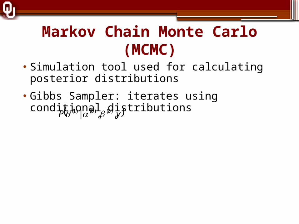
Markov Chain Monte Carlo (MCMC)
• Simulation tool used for calculating posterior distributions
• Gibbs Sampler: iterates using conditional distributions
yP ,,| )0()0()1(

Markov Chain Monte Carlo (MCMC)
• Simulation tool used for calculating posterior distributions
• Gibbs Sampler: iterates using conditional distributions
yP ,,| )0()0()1(
xyP ,,~,,,,|~ )0()0()0()0()1()1(

Markov Chain Monte Carlo (MCMC)
• Simulation tool used for calculating posterior distributions
• Gibbs Sampler: iterates using conditional distributions
yP ,,| )0()0()1(
xyP ,,~,,,,|~ )0()0()0()0()1()1(
yP ,,,,~| )0()0()1()1()1(

Markov Chain Monte Carlo (MCMC)
• Simulation tool used for calculating posterior distributions
• Gibbs Sampler: iterates using conditional distributions
• Software▫Bayesian Inference Using Gibbs Sampling (BUGS)▫ Just Another Gibbs Sampler (JAGS)
yP ,,| )0()0()1(
xyP ,,~,,,,|~ )0()0()0()0()1()1(
yP ,,,,~| )0()0()1()1()1(
yxrsP ,,,,~,,~| )0()1()1()1(

Toy Example

Parameters for Priors
1,1~~ LogNj 1,1~~ LogNj

Large Gamma Needed

Resultsgamma chains 1:2
iteration
501 750 1000 1250 1500
60.0
80.0
100.0
120.0
140.0
160.0
theta[1] chains 1:2
iteration
501 750 1000 1250 1500
0.0
0.25
0.5
0.75
1.0

Test Data Automatically Calculated
theta[81] chains 1:2
iteration
501 750 1000 1250 1500
0.0
0.25
0.5
0.75
1.0
Mean St Dev 2.5% Median 97.5%
α81 1.54 0.41 0.94 1.47 2.49
β 81 0.83 0.24 0.48 0.79 1.44
θ 81 0.65 0.27 0.08 0.70 1.00

Comparison
Beta SVM RVM1s correctly classified
(19 total 1s)14 14 0
0s correctly classified(21 total 0s)
17 17 21
γ 109 6.67 0.586

Conclusion
•Advantages of Beta-Bayesian Method▫Incorporate non-Gaussian process▫Results of example equal to SVM▫Testing data automatically calculated with MCMC
•Disadvantages▫MCMC slow algorithm▫Analytical solution may not be possible▫Difficult to determine prior distributions
•Future Work▫Real data▫More comparisons with existing methods
References
•Cameron A. MacKenzie, Theodore B. Trafalis and Kash Barker, “A Bayesian Beta Kernel Model for Binary Classification and Online Learning Problems”, Statistical Analysis and Data Mining, Vol. (In press 2014)