1 cisc 841 bioinformatics (fall 2007) kernel engineering and applications of svms

1

CISC 841 Bioinformatics(Fall 2007)

Kernel engineering and applications of SVMs

2

Kernels

Given a mapping Φ( ) from the space of input vectors to some higher dimensional feature space, the kernel K of two vectors xi, xj is the inner product of their images in the feature space, namely,

K(xi, xj) = Φ (xi)·Φ (xj ).

Since we just need the inner product of vectors in the feature space to find the maximal margin separating hyperplane, we use the kernel in place of the mapping Φ( ).

Because inner product of two vectors is a measure of the distance between the vectors, a kernel function actually defines the geometry of the feature space (lengths and angles), and implicitly provides a similarity measure for objects to be classified.

3

Mercer’s condition

Since kernel functions play an important role, it is important to know if a kernel gives dot products (in some higher dimension space).

For a kernel K(x,y), if for any g(x) such that g(x)2 dx is finite, we have

K(x,y)g(x)g(y) dx dy 0,then there exist a mapping such that

K(x,y) = (x) · (y)Notes:

1. Mercer’s condition does not tell how to actually find .2. Mercer’s condition may be hard to check since it must hold for

every g(x).

4

More kernel functionssome commonly used generic kernel functions

5

Advanced Issues– Soft margin

• Allow misclassification, but with penalties

– Multiclass classification• Indirect: combine multiple binary classifiers into a

single multiclass classifier

• Direct: generalize binary classification methods

– SVM Regression– Unsupervised learning: Support vector

clustering by Ben-Hur et al (2001)

Soft margin

6

7

How to construct a kernel?

11

• Diffusion kernels for graphsK = exp(- L)

where is a constant, and L = D – A is the Laplacian matrix (D is the diagonal degree matrix and A is the adjacent matrix for the graph).

Intuition: two nodes get closer in the feature space if there are many short paths connecting them in the graph.

CISC667, F05, Lec23, Liao 12

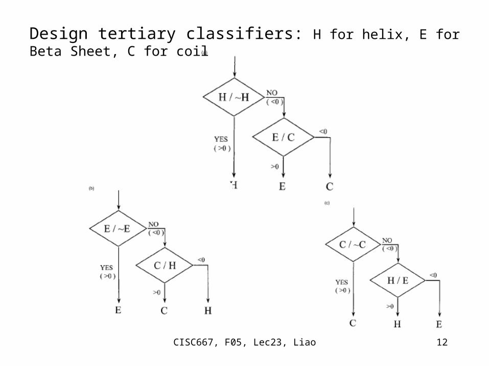
Design tertiary classifiers: H for helix, E for Beta Sheet, C for coil


Nguyen & Rajapakse, Genome Informatics 14: 218-227 (2003)


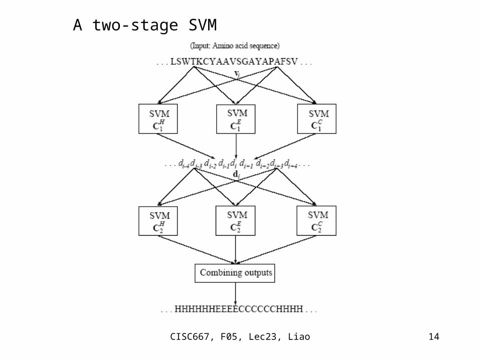
A two-stage SVM

15

Applications in Bioinformatics

• W. Noble, “Support vector machine applications in computational biology”, Kernel Methods in Computational Biology. B. Schoelkopf, K. Tsuda and J.-P. Vert, ed. MIT Press, 2004.

18

SVM-Fisher method

Protein homologs

HMMProtein non-

homologs

Positivegradientvectors

Negativegradientvectors

Support vector machine

Binary classification

Target protein of unknown function

1

2

34

Positive train Negative train

Testing data

19

HMM gradients

• Fisher Score <X> = log P(X|H, )

• The gradient of a sequence X with respect to a given model is computed using the forward-backward algorithm.

• Each dimension corresponds to one parameter of the model.

• The feature space is tailored to the sequences from which the model was trained.

20

Combining pairwise similarity with SVMs for protein homology detection

Protein homologs

Protein non-homologs

Positivepairwise score

vectors

Negativepairwise score

vectors

Support vector machine

Binary classification

Target protein of unknown function

1

23

Positive train Negative train

Testing data

21

Experiment: known protein families

Jaakkola, Diekhans and Haussler 1999

22

Vectorization

24

A measure of sensitivity and specificity

ROC = 1

ROC = 0

ROC = 0.67

6

5

ROC: receiver operating characteristic score is the normalized area

under a curve the plots true positives as a function of false positives

25

Performance Comparison (1)

26

Using Phylogenetic Profiles & SVMs YAL001C

E-value Phylogenetic profile

0.122 1

1.064 0

3.589 0

0.008 1

0.692 1

8.49 0

14.79 0

0.584 1

1.567 0

0.324 1

0.002 1

3.456 0

2.135 0

0.142 1

0.001 1

0.112 1

1.274 0

0.234 1

4.562 0

3.934 0

0.489 1

0.002 1

2.421 0

0.112 1

27

phylogenetic profiles and Evolution Patterns1

1

1 1

10

0

1 1 0 1 0 0 0 1 1 0x

Impossible to know for sure if the gene followed exactly this

evolution pattern

28

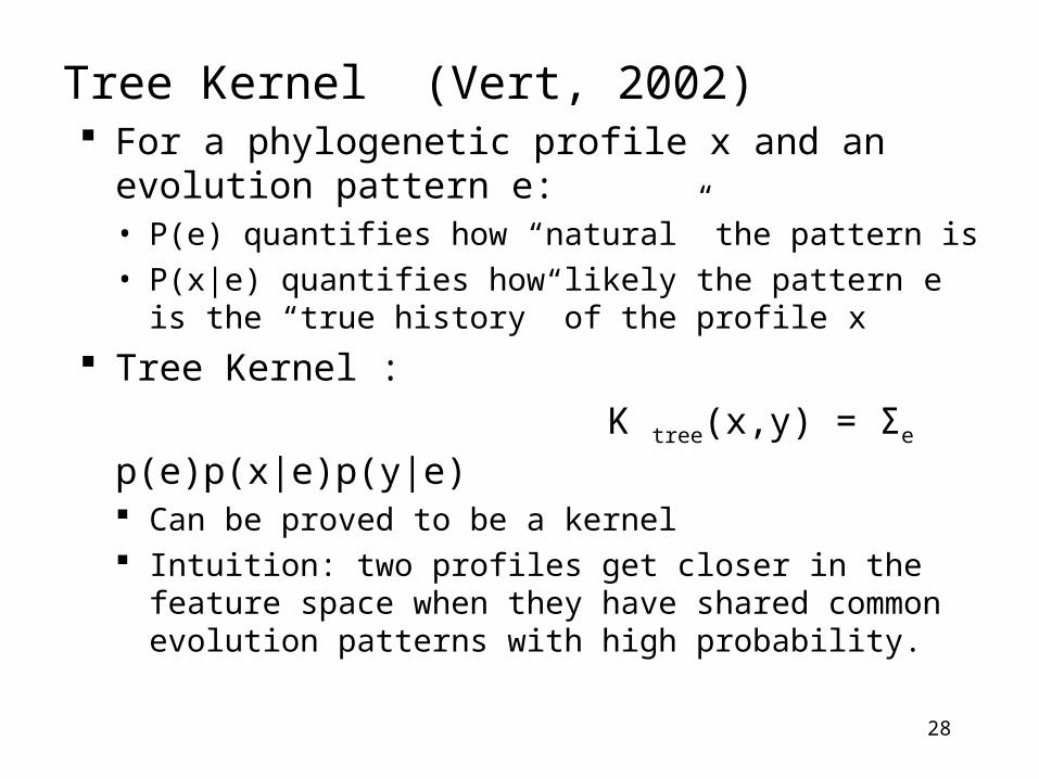
Tree Kernel (Vert, 2002) For a phylogenetic profile x and an evolution pattern e:• P(e) quantifies how “natural” the pattern is

• P(x|e) quantifies how likely the pattern e is the “true history” of the profile x

Tree Kernel :

K tree(x,y) = Σe p(e)p(x|e)p(y|e) Can be proved to be a kernel Intuition: two profiles get closer in the feature space when

they have shared common evolution patterns with high probability.

29

Tree-Encoded Profile (Narra & Liao, 2004)

1 1 0 1 0 0 0 1 1 0

1

00.33

0.67

0.34

0.5

0.75

0.55

0 1 0.33 0.5 0.67 0.75 0.34 0.55

30

Tree Encoded Polynomial kernel

Prediction of Protein-Protein Interactions

based on co-evolution (correlated mutations)

Credit: Valencia & Pazos

Mirror Tree (Pazos and Valencia, 2001)

Li Liao, 09/13/2006 33

A B C D E F G HABCDEFGH

00

00

00

0

0

00

0

0

( )…. ( )

section1

….

section2

section2

….

….

Method: TreeSec

Li Liao, DuPont CR&D, 08/17/2007 34

Hybrid/Composite Kernel

Two alternative views:

• as a hybrid that employs in tandem both an explicit mapping: phylogenetic vector super-phylogenetic vector

x T(x) and a generic kernel

K(a, b) = exp[ - |a-b|2]

• or as a conventional SVM but with a specially engineered kernel that is composed of the two steps above

K’(x, y) = exp [-|T(x) - T(y)|2]

Classification Data representation ROC

Unsupervised(Pearson CC)

MirrorTree 0.6587

TreeSec 0.6731

Polynomial kernel SVM

MirrorTree 0.7067

TreeSec 0.7452

TreeSec x 10 0.8446

TreeSec x 10 (no NJ) 0.6907

TreeSec x 10 (random tree)

0.5529

Results:

Dataset (Sato, et al, 2005)13 pairs of interacting proteins from E. coli. (DIP)41 bacterial genomes are selected from KEGG/KO (Kanehisa et al, 2004).

Cross validation experiments: leave-one-out


m

d

ddd yxK

1

)( yx,

Linear Kernel with Adaptive Weights

Kernel: K(x, y) = (x) · (y)

Linear kernel: K(x,y) = x y

Weighted Linear Kernel:

= ?


]22

[min 2

,,

ii

ebwe

ww

ii eby 1)( ixw

N

kkk

Tkk

ii ebxwyeebwL

1

2 }1])([{]22

[);,,( ww

1if1 iybixw

1if1 iybixw

1)( byi ixw

Least Squares SVM (Suykens & Vandewalle, 1999)


iiiy

w

Lixw 0

00

iiiy

b

L

nto1i,0

iii

ee

L

nto1i,01][0

iii

ebyL

jxw

nto1i,1][1

,

j

n

j

jijii yyby

ji xx

ji xx ji yy


j d

jjid

jd

idjii xxyyby 1])([ ,

nto1i,1][ , djj d

jidj

dijii xxyyby

j d

djjy 0

Adaptive Weights

Weights ’s can be obtained, simultaneously with ’s, from solving the above linear equations.


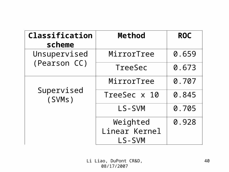
Classification scheme

Method ROC

Unsupervised(Pearson CC)

MirrorTree 0.659

TreeSec 0.673

Supervised(SVMs)

MirrorTree 0.707

TreeSec x 10 0.845

LS-SVM 0.705

Weighted Linear Kernel

LS-SVM

0.928

41

References and resources

• www.kernel-machines.org

– SVMLight

• W. Noble, “Support vector machine applications in computational biology”, Kernel Methods in Computational Biology. B. Schoelkopf, K. Tsuda and J.-P. Vert, ed. MIT Press, 2004.

• Craig RA and Liao L. BMC Bioinformatics, 2007, 8:6.

• Craig RA and Liao L. Improving Protein-Protein Interaction Prediction based on Phylogenetic Information using Least-Squares SVM. Ann. NY Acad. Sci. (in press)

http://www.kernel-machines.org/

1 cisc 841 bioinformatics (fall 2007) kernel engineering and applications of svms

Documents