Structural Analysis - II

Indeterminate structures; Force method of analysis

Module I

Statically and kinematically indeterminate structures

• Degree of static indeterminacy, Degree of kinematic indeterminacy, Force and displacement method of analysis

Force method of analysis

•Method of consistent deformation-Analysis of fixed and continuous beams

•Clapeyron’s theorem of three moments-Analysis of fixed and continuous beams

•Principle of minimum strain energy-Castigliano’s second theorem- Analysis of beams, plane trusses and plane frames.

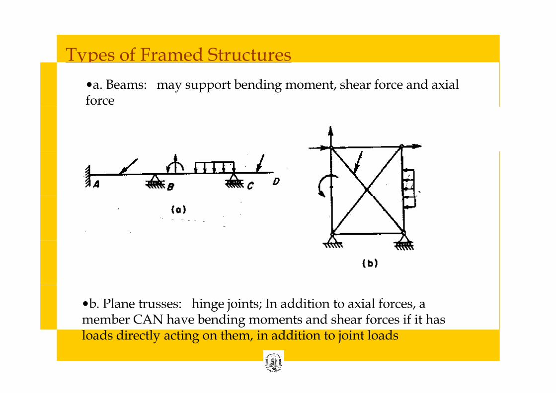
Types of Framed Structures

•a. Beams: may support bending moment, shear force and axial force

•b. Plane trusses: hinge joints; In addition to axial forces, a member CAN have bending moments and shear forces if it has loads directly acting on them, in addition to joint loads

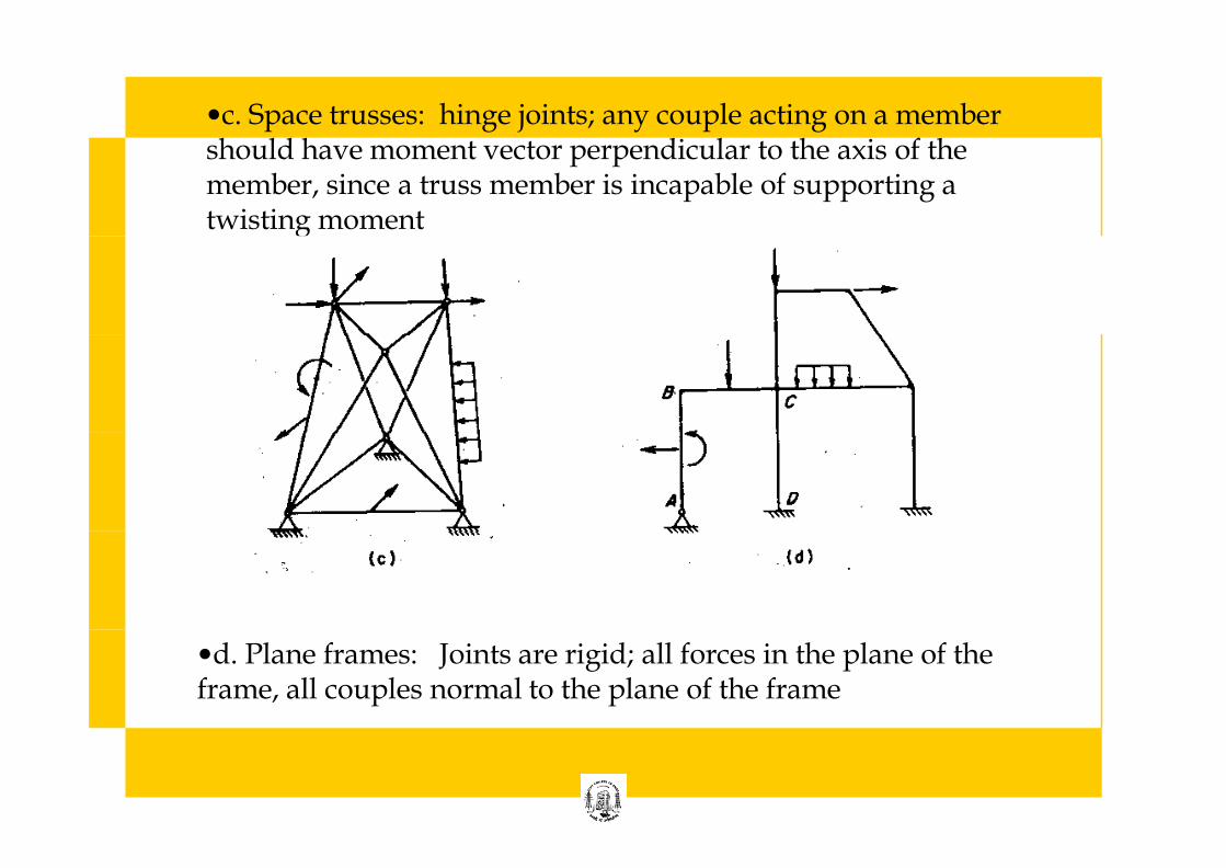
•c. Space trusses: hinge joints; any couple acting on a member should have moment vector perpendicular to the axis of the member, since a truss member is incapable of supporting a twisting moment

•d. Plane frames: Joints are rigid; all forces in the plane of the frame, all couples normal to the plane of the frame

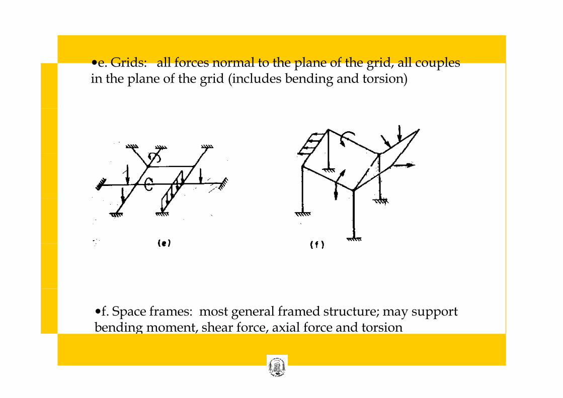
•e. Grids: all forces normal to the plane of the grid, all couples in the plane of the grid (includes bending and torsion)

•f. Space frames: most general framed structure; may support bending moment, shear force, axial force and torsion

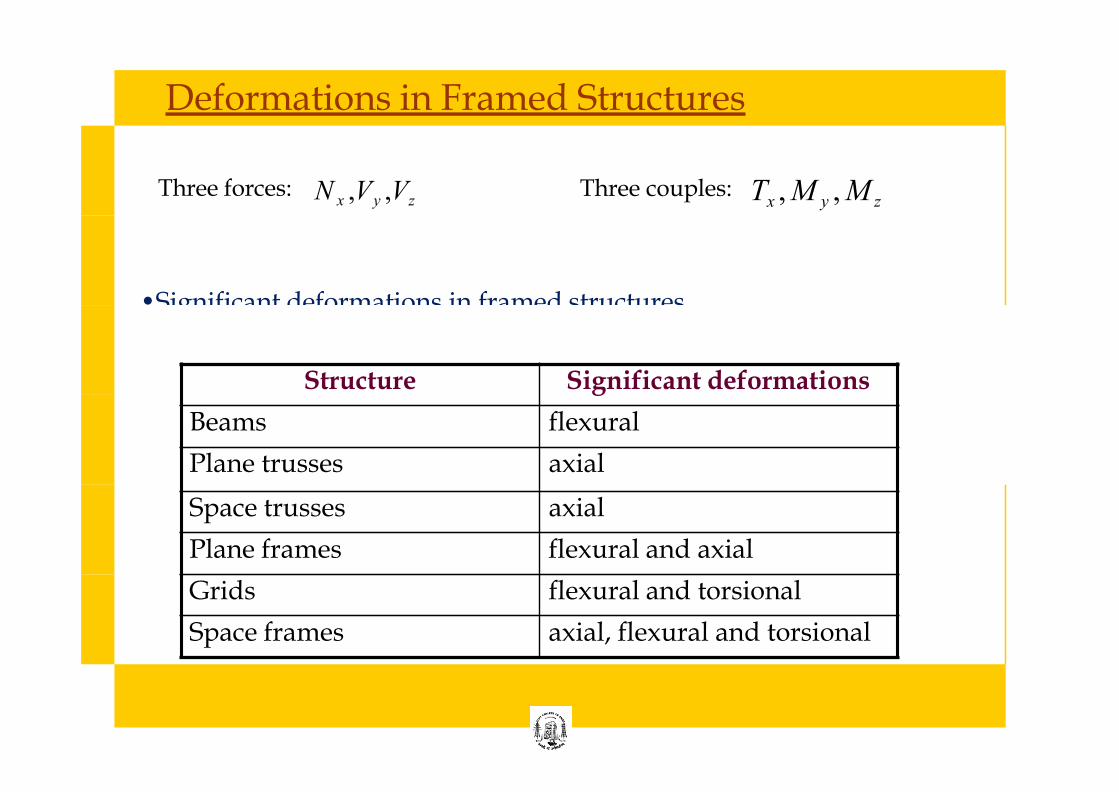
Deformations in Framed Structures

Tx , M y , M z Three couples: N x ,Vy ,Vz

Three forces:

•Significant deformations in framed structures

Structure Significant deformations

Beams flexural

Plane trusses axial

Space trusses axial

Plane frames flexural and axial

Grids flexural and torsional

Space frames axial, flexural and torsional

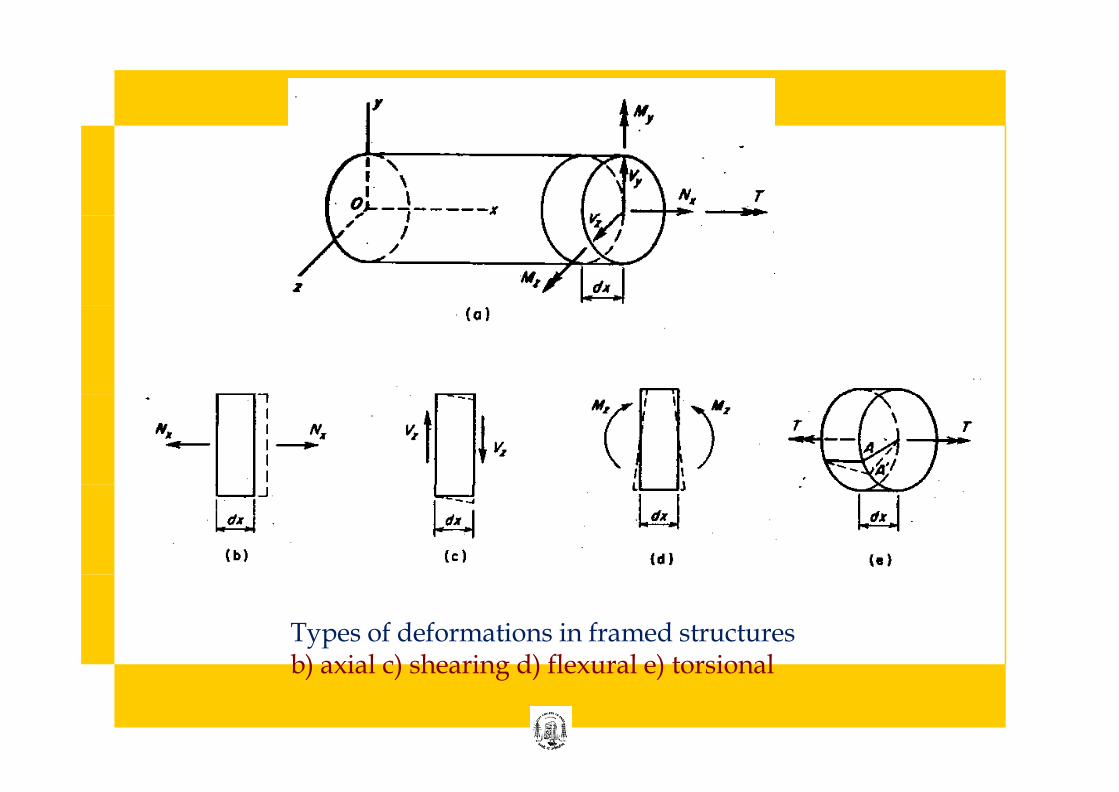
Types of deformations in framed structures b) axial c) shearing d) flexural e) torsional

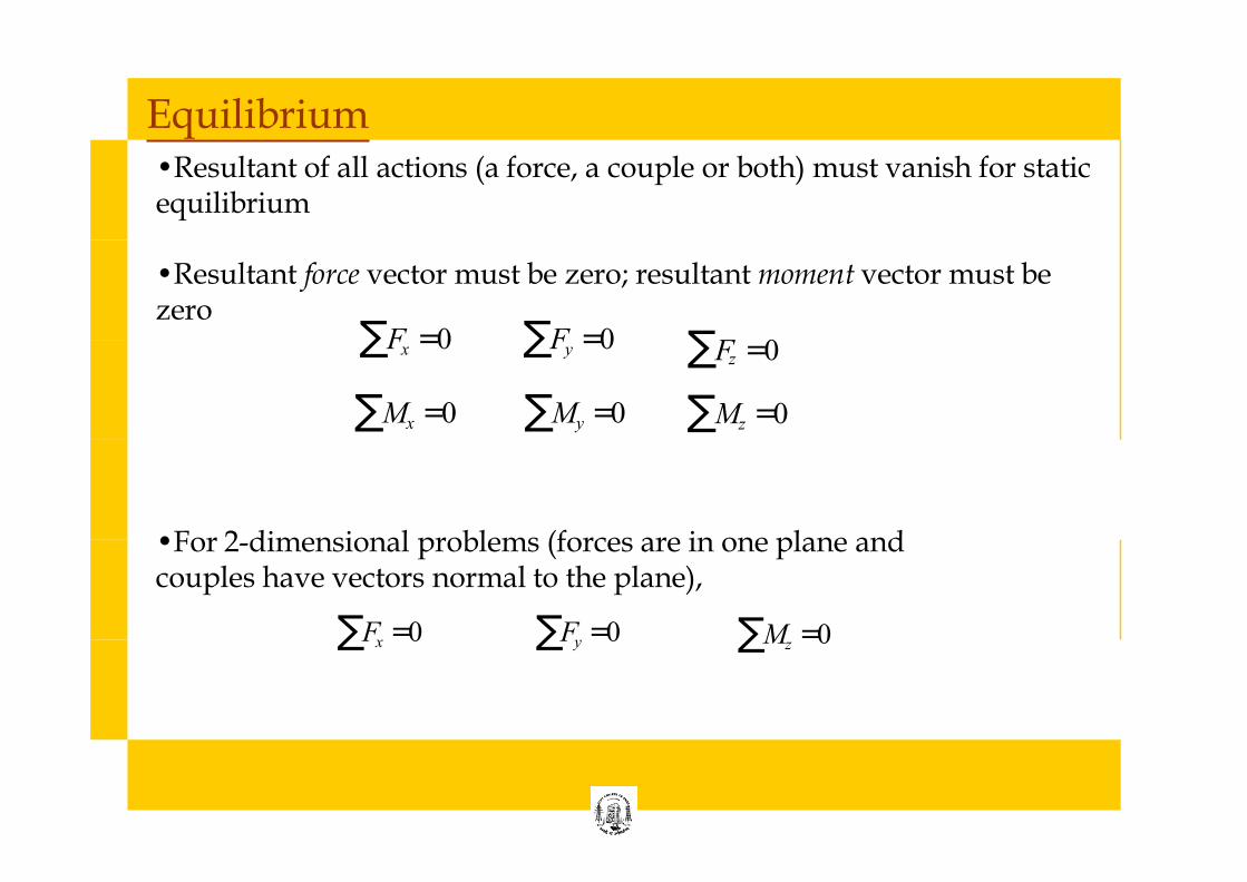
Equilibrium

•Resultant of all actions (a force, a couple or both) must vanish for static equilibrium

•Resultant force vector must be zero; resultant moment vector must be zero

∑Fx = 0

∑Mx = 0

∑Fy = 0

∑My =0

F = 0 ∑ z

∑Mz = 0

∑Fx =0 ∑Fy =0

•For 2-dimensional problems (forces are in one plane and couples have vectors normal to the plane),

∑Mz =0

Compatibility

•Compatibility conditions: Conditions of continuity of displacements throughout the structure

•Eg: at a rigid connection between two members, the displacements (translations and rotations) of both members must be the same

9

Indeterminate Structures

Force method and Displacement method

• Force method (Flexibility method)

• Actions are the primary unknowns

• Static indeterminacy: excess of unknown actions than the available number of equations of static equilibrium

• Displacement method (Stiffness method)

•Displacements of the joints are the primary unknowns

•Kinematic indeterminacy: number of independent translations and rotations

Static indeterminacy

• Beam:

•Static indeterminacy = Reaction components - number of eqns available E = R − 3

• Examples:

•Single span beam with both ends hinged with inclined loads • Continuous beam • Propped cantilever • Fixed beam

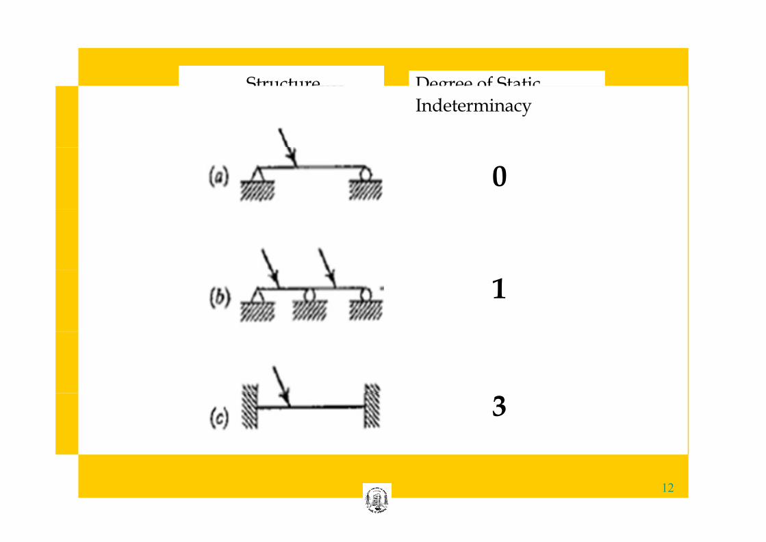
Degree of Static Structure Indeterminacy

0

1

3

12

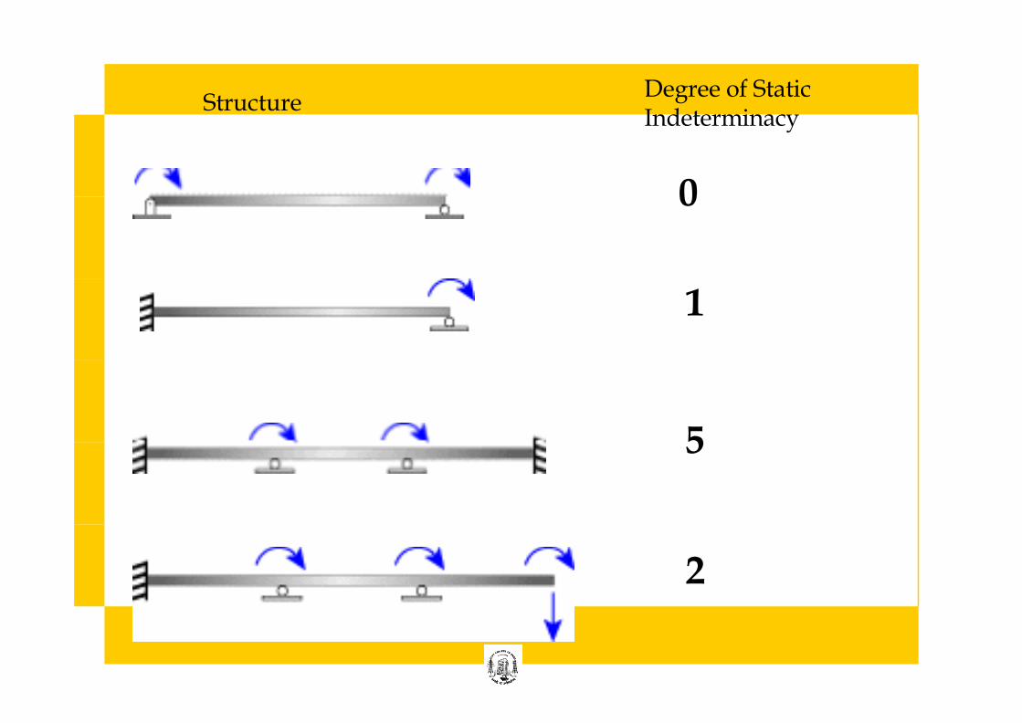
Degree of Static Indeterminacy

Structure

0

1

5

2

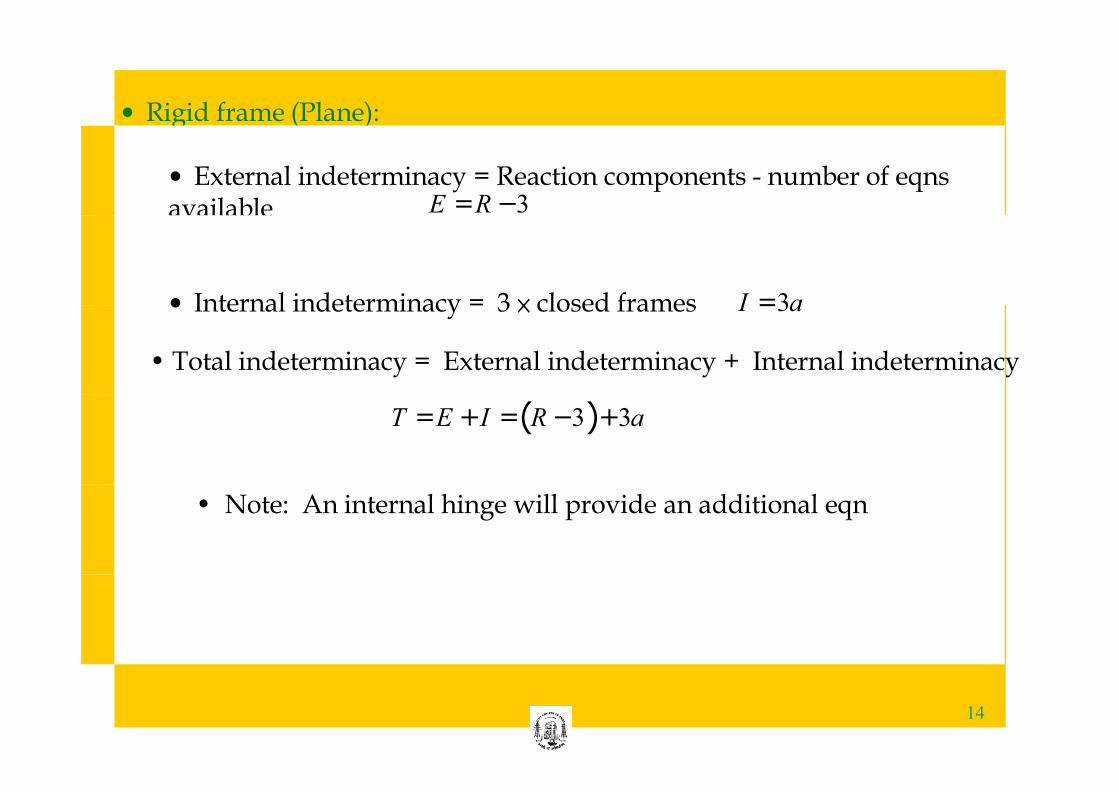
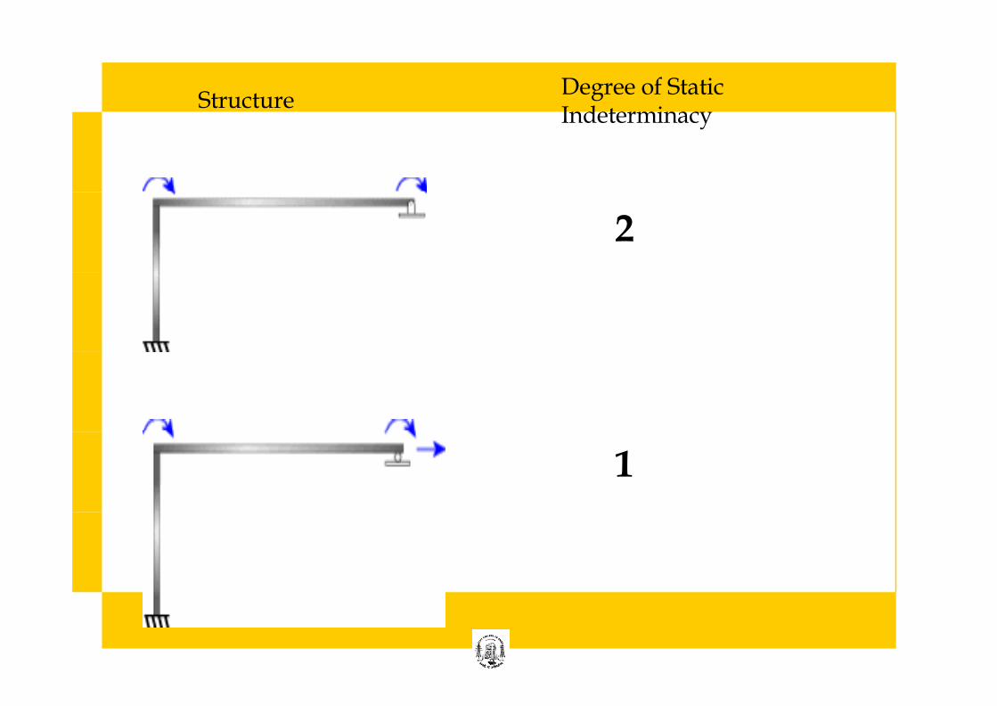
• Rigid frame (Plane):

• External indeterminacy = Reaction components - number of eqns available E = R − 3

• Internal indeterminacy = 3 × closed frames I = 3a

• Total indeterminacy = External indeterminacy + Internal indeterminacy

T = E + I = (R − 3) + 3a

• Note: An internal hinge will provide an additional eqn

14

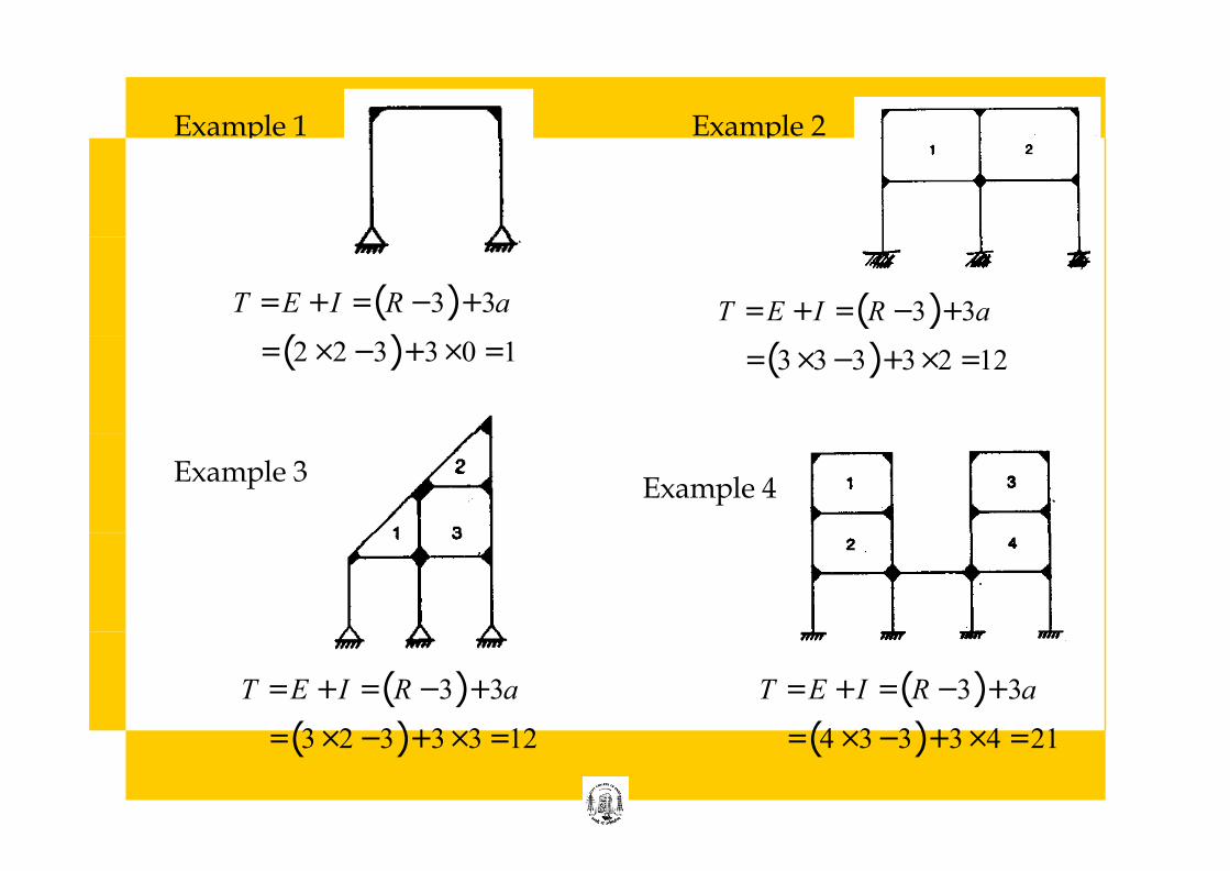
Example 1 Example 2

T = E + I = (R − 3) + 3a

= (3 × 3 − 3) + 3 × 2 = 12

T = E + I = (R − 3) + 3a

= (2 × 2 − 3) + 3 × 0 = 1

Example 3 Example 4

T = E + I = (R − 3) + 3a

= (3 × 2 − 3) + 3 × 3 = 12

T = E + I = (R − 3) + 3a

= (4 × 3 − 3) + 3 × 4 = 21

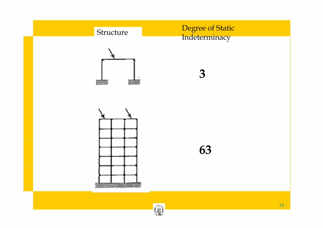
Degree of Static Structure

Indeterminacy

3

63

16

Degree of Static Indeterminacy

Structure

2

1

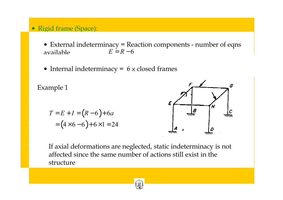
• Rigid frame (Space):

• External indeterminacy = Reaction components - number of eqns available E = R − 6

• Internal indeterminacy = 6 × closed frames

Example 1

T = E + I = (R − 6) + 6a

= (4 × 6 − 6) + 6 ×1 = 24

If axial deformations are neglected, static indeterminacy is not affected since the same number of actions still exist in the structure

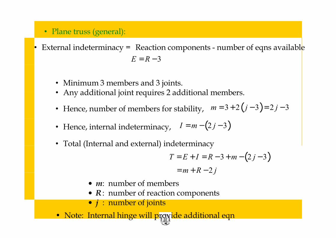
• Plane truss (general):

• External indeterminacy = Reaction components - number of eqns available

E = R − 3

• Minimum 3 members and 3 joints. • Any additional joint requires 2 additional members.

m = 3 + 2 ( j − 3) = 2 j − 3 • Hence, number of members for stability,

I = m − (2 j − 3) • Hence, internal indeterminacy,

• Total (Internal and external) indeterminacy

T = E + I = R − 3 + m − (2 j − 3)

= m + R − 2 j

• m: number of members • R : number of reaction components • j : number of joints

• Note: Internal hinge will provide additional eqn

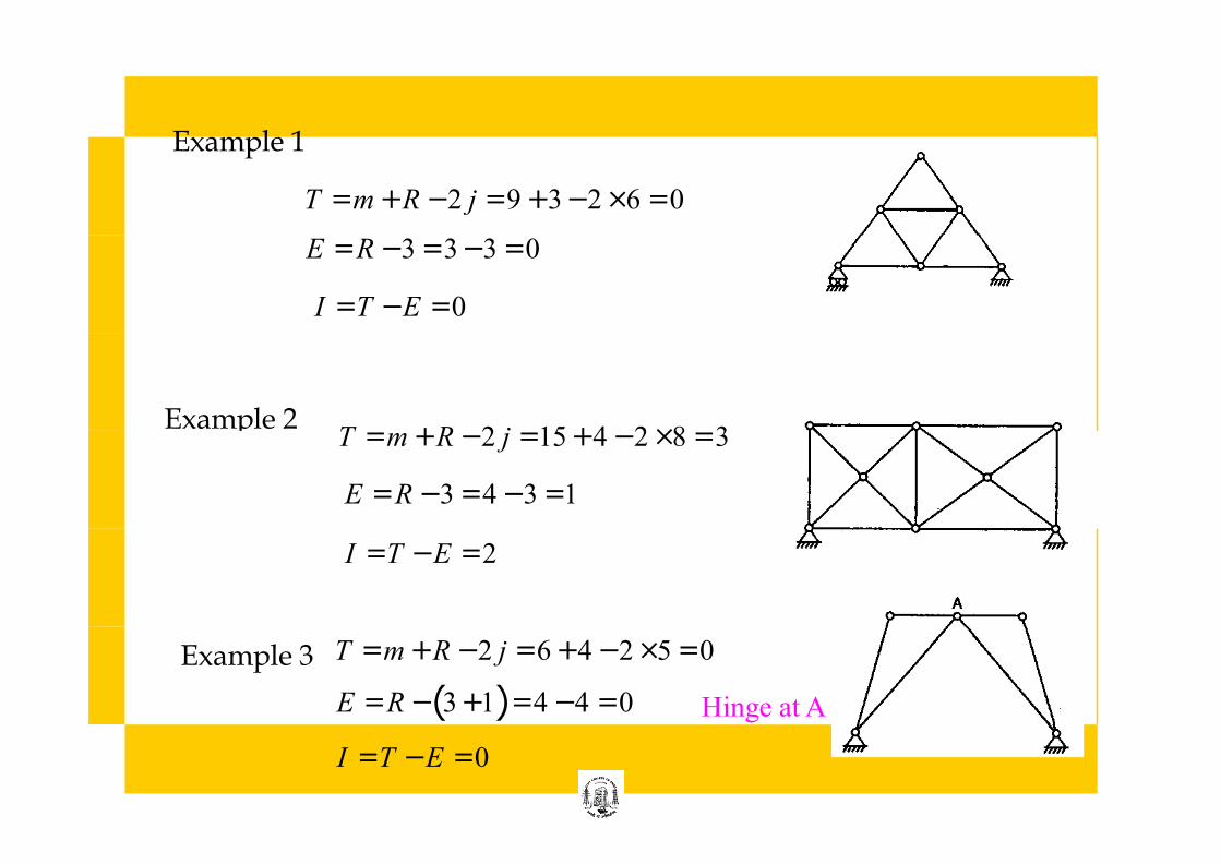
Example 1

T = m + R − 2 j = 9 + 3 − 2 × 6 = 0

E = R − 3 = 3 − 3 = 0

I = T − E = 0

Example 2 T = m + R − 2 j = 15 + 4 − 2 × 8 = 3

E = R − 3 = 4 − 3 = 1

I = T − E = 2

Example 3 T = m + R − 2 j = 6 + 4 − 2 × 5 = 0

E = R − (3 + 1) = 4 − 4 = 0 Hinge at A

I = T − E = 0

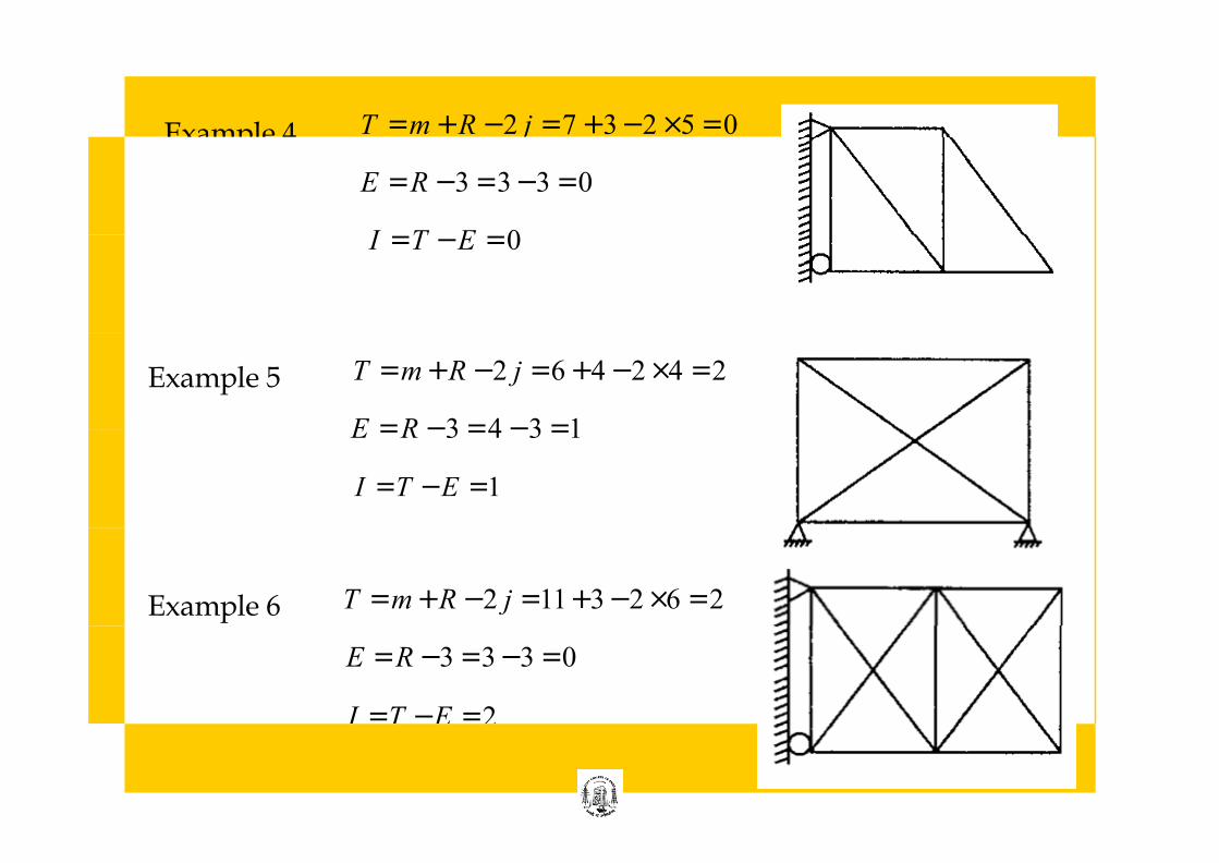
Example 4 T = m + R − 2 j = 7 + 3 − 2 × 5 = 0

E = R − 3 = 3 − 3 = 0

I = T − E = 0

T = m + R − 2 j = 6 + 4 − 2 × 4 = 2

E = R − 3 = 4 − 3 = 1

Example 5

I = T − E = 1

T = m + R − 2 j = 11 + 3 − 2 × 6 = 2

E = R − 3 = 3 − 3 = 0

I = T − E = 2

Example 6

• Wall or roof attached pin jointed plane truss (Exception to the above general case):

•Internal indeterminacy I = m − 2 j

•External indeterminacy = 0 (Since, once the member forces are determined, reactions are determinable)

Example 1 Example 3 Example 2

T = I = m − 2 j

= 6 − 2 × 3 = 0

T = I = m − 2 j

= 5 − 2 ×1 = 3 T = I = m − 2 j

= 7 − 2 × 3 = 1

22

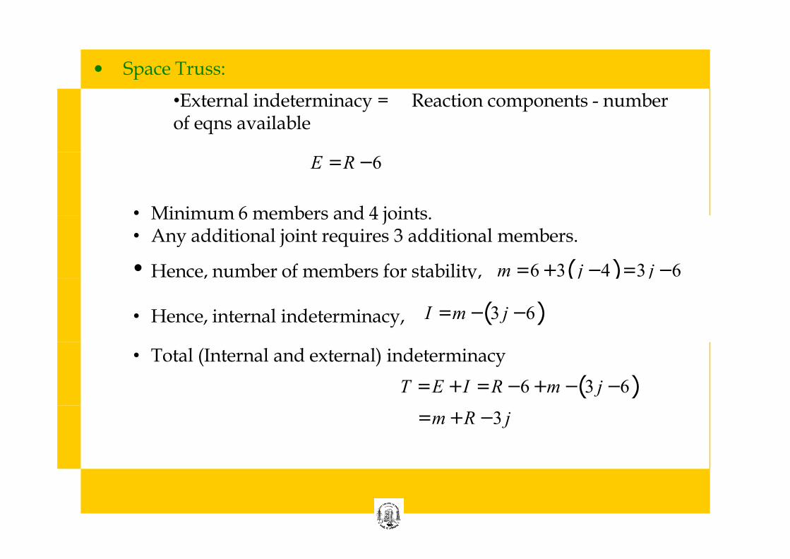
• Space Truss:

•External indeterminacy = Reaction components - number of eqns available

E = R − 6

• Minimum 6 members and 4 joints. • Any additional joint requires 3 additional members.

• Hence, number of members for stability, m = 6 + 3( j − 4) = 3 j − 6

I = m − (3 j − 6) • Hence, internal indeterminacy,

• Total (Internal and external) indeterminacy

T = E + I = R − 6 + m − (3 j − 6)

= m + R − 3 j

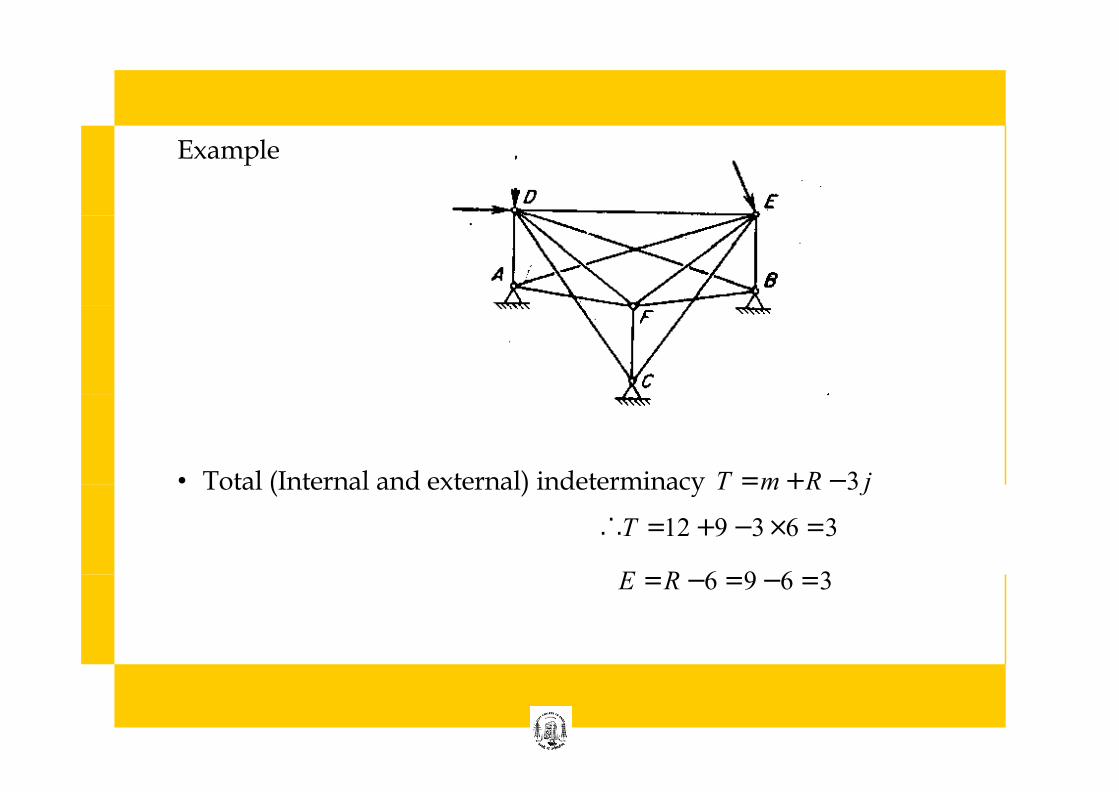
Example

• Total (Internal and external) indeterminacy T = m + R − 3 j

∴T = 12 + 9 − 3 × 6 = 3

E = R − 6 = 9 − 6 = 3

Kinematic indeterminacy

• joints: where members meet, supports, free ends • joints undergo translations or rotations

•in some cases joint displacements will be known, from the restraint conditions •the unknown joint displacements are the kinematically indeterminate quantities

odegree of kinematic indeterminacy: number of degrees of freedom

Two types of DOF

• Nodal type DOF • Joint type DOF

25

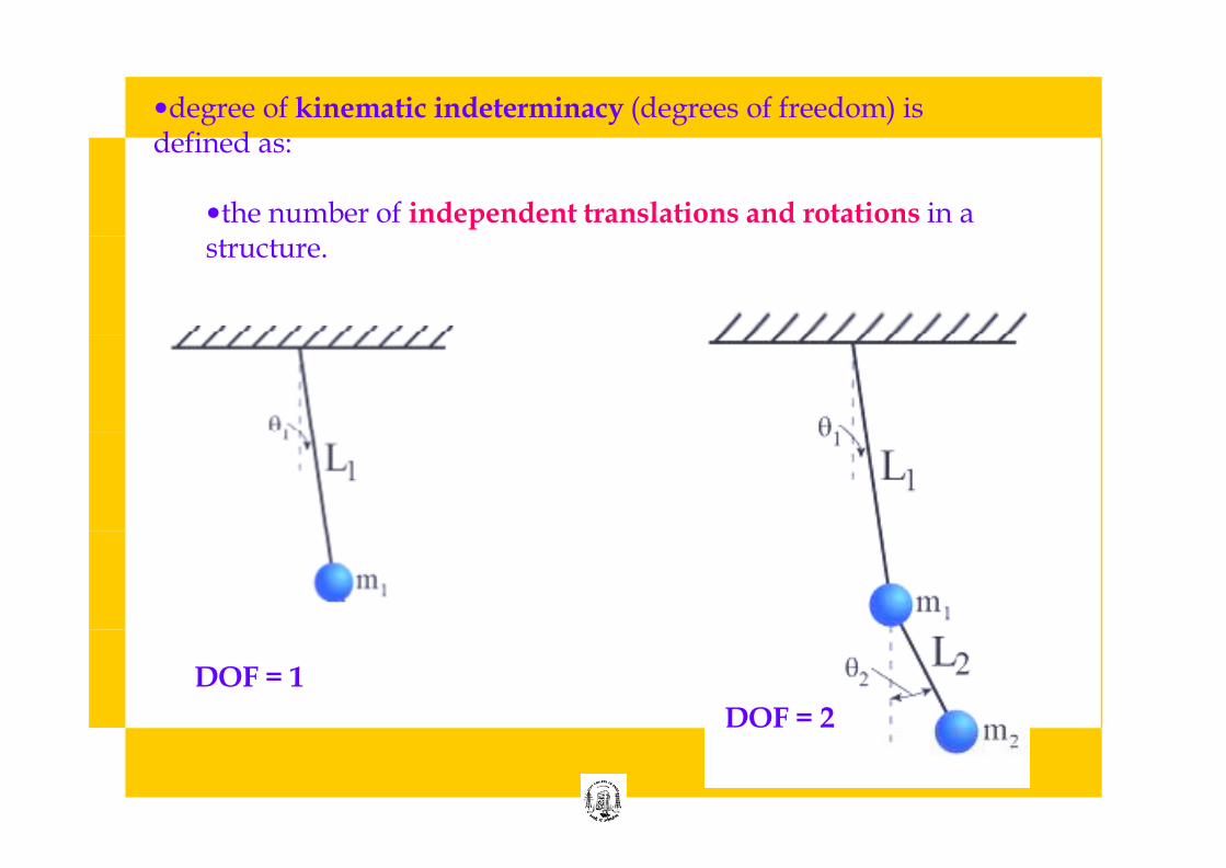
•degree of kinematic indeterminacy (degrees of freedom) is defined as:

•the number of independent translations and rotations in a structure.

DOF = 1

DOF = 2

•in a truss, the joint rotation is not regarded as a degree of freedom. joint rotations do not have any physical significance as they have no effects in the members of the truss

•in a frame, degrees of freedom due to axial deformations can be neglected

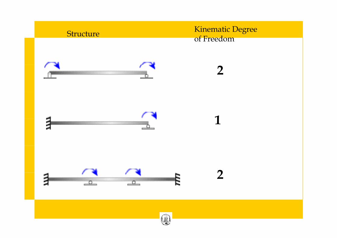
Kinematic Degree of Freedom

Structure

2

1

2

Kinematic Degree of Freedom

Structure

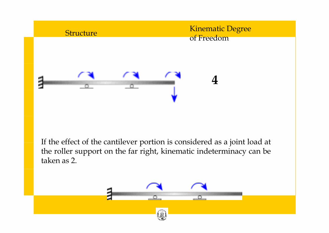
4

If the effect of the cantilever portion is considered as a joint load at the roller support on the far right, kinematic indeterminacy can be taken as 2.

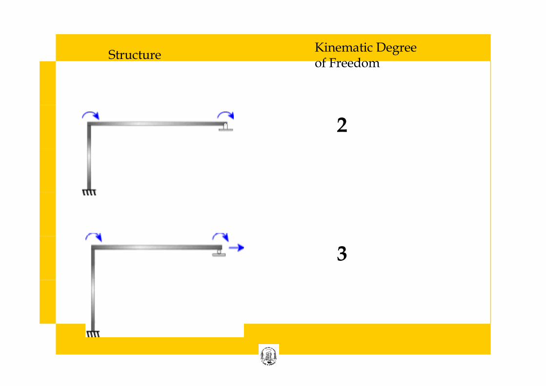
Kinematic Degree of Freedom

Structure

2

3

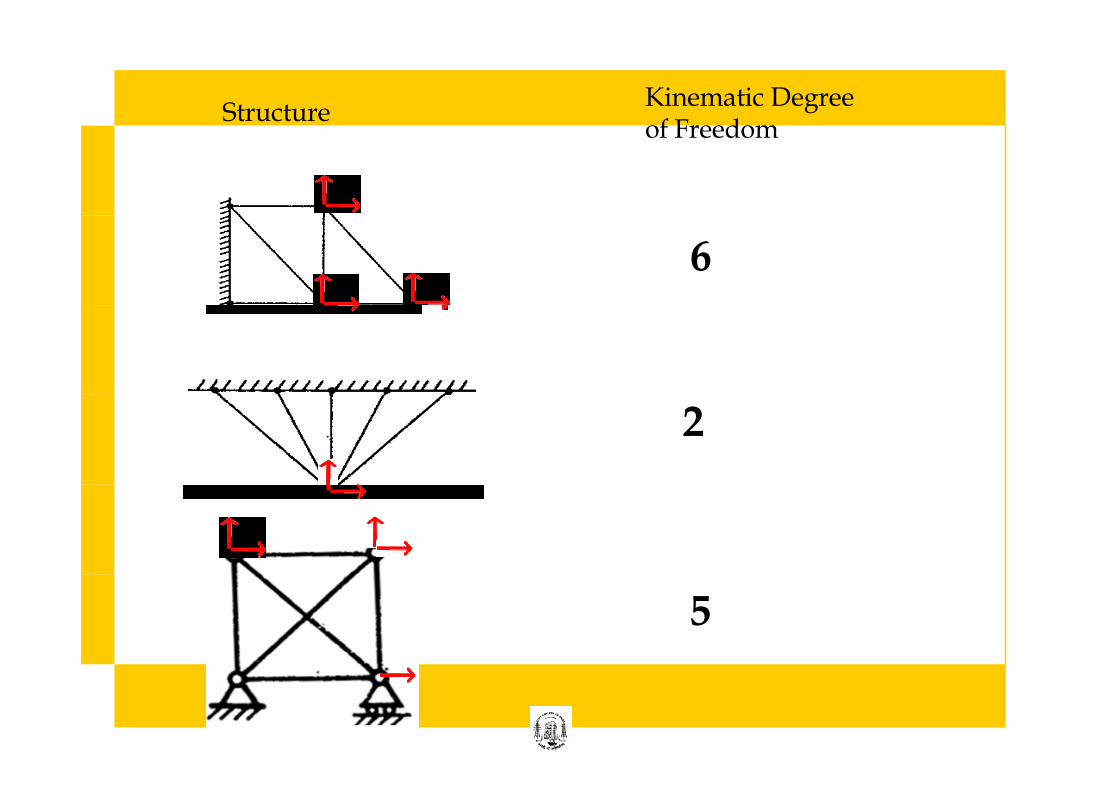
Kinematic Degree of Freedom

Structure

6

2

5

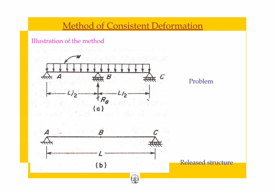
Method of Consistent Deformation

Illustration of the method

Problem

Released structure

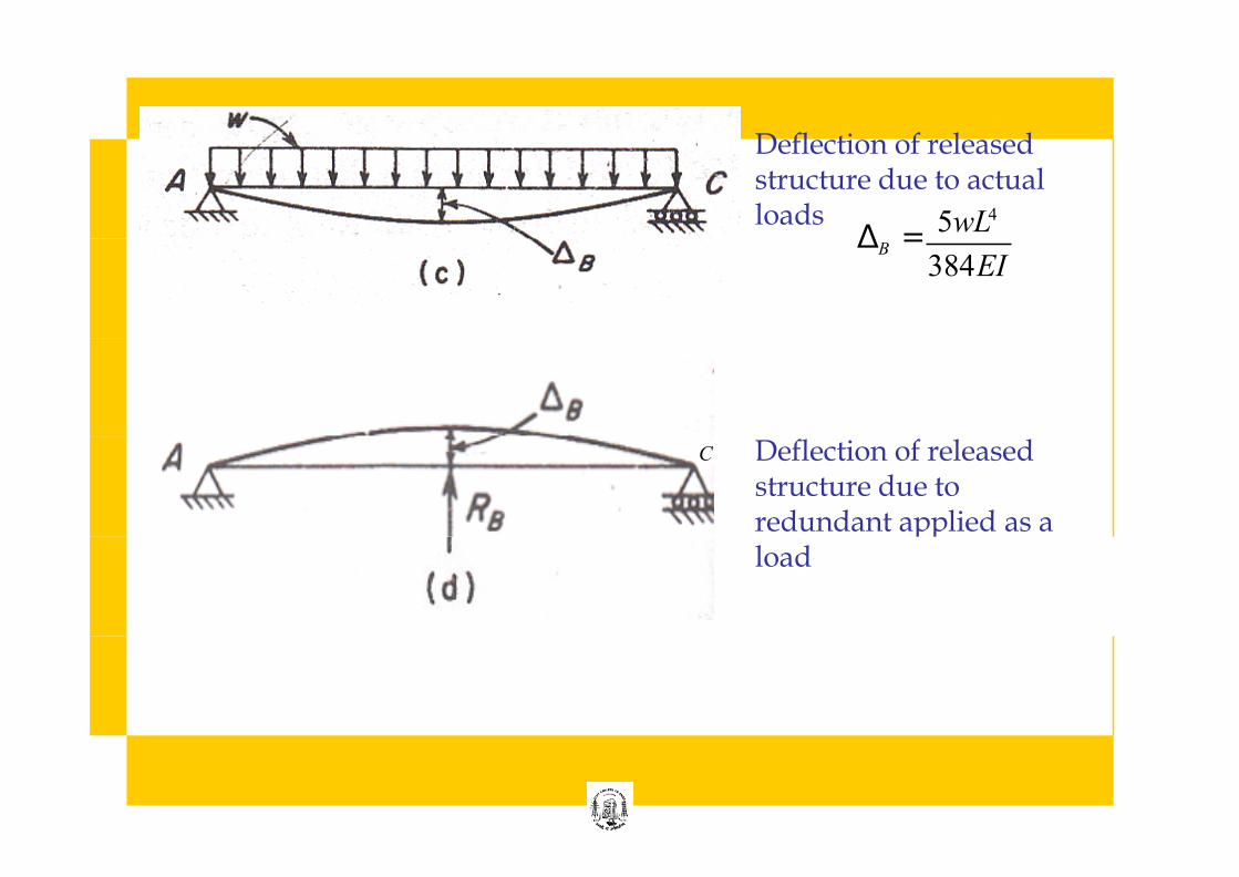
5wL4

Deflection of released structure due to actual loads

384EI ΔB =

C Deflection of released structure due to redundant applied as a load

R L3

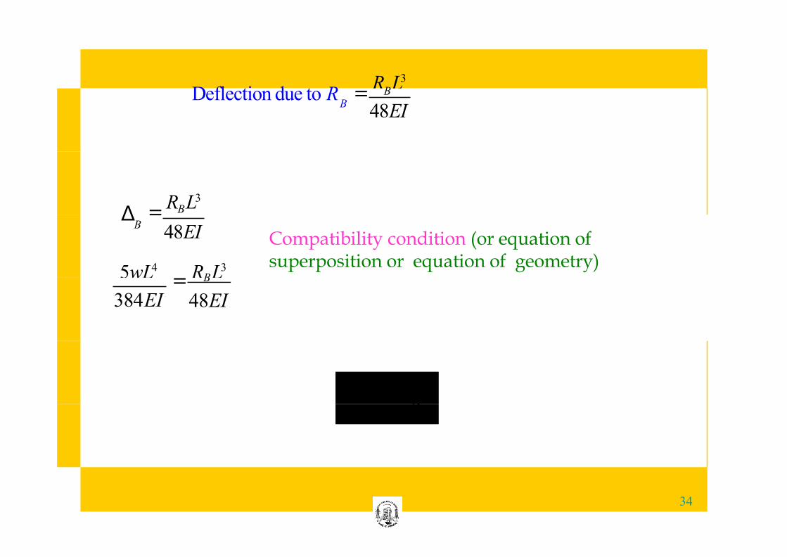
Deflection due to R = 48EI

B B

3

= RB L

48EI B

Δ

5wL4 R L3

Compatibility condition (or equation of superposition or equation of geometry)

384EI = B

48EI

∴ R = 5wL

B 8

34

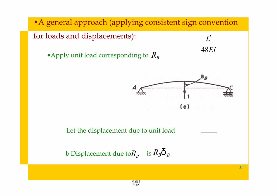
•A general approach (applying consistent sign convention

for loads and displacements):

•Apply unit load corresponding to RB

Let the displacement due to unit load

b Displacement due toRB is RBδB

L3

48EI

35

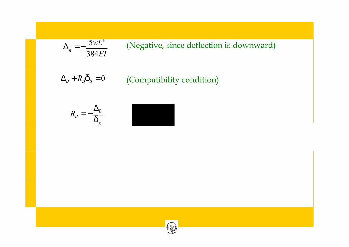
5wL4

384EI B

Δ = − (Negative, since deflection is downward)

ΔB + RBδB = 0 (Compatibility condition)

ΔB RB =− δ

∴ R = 5wL

B 8 B

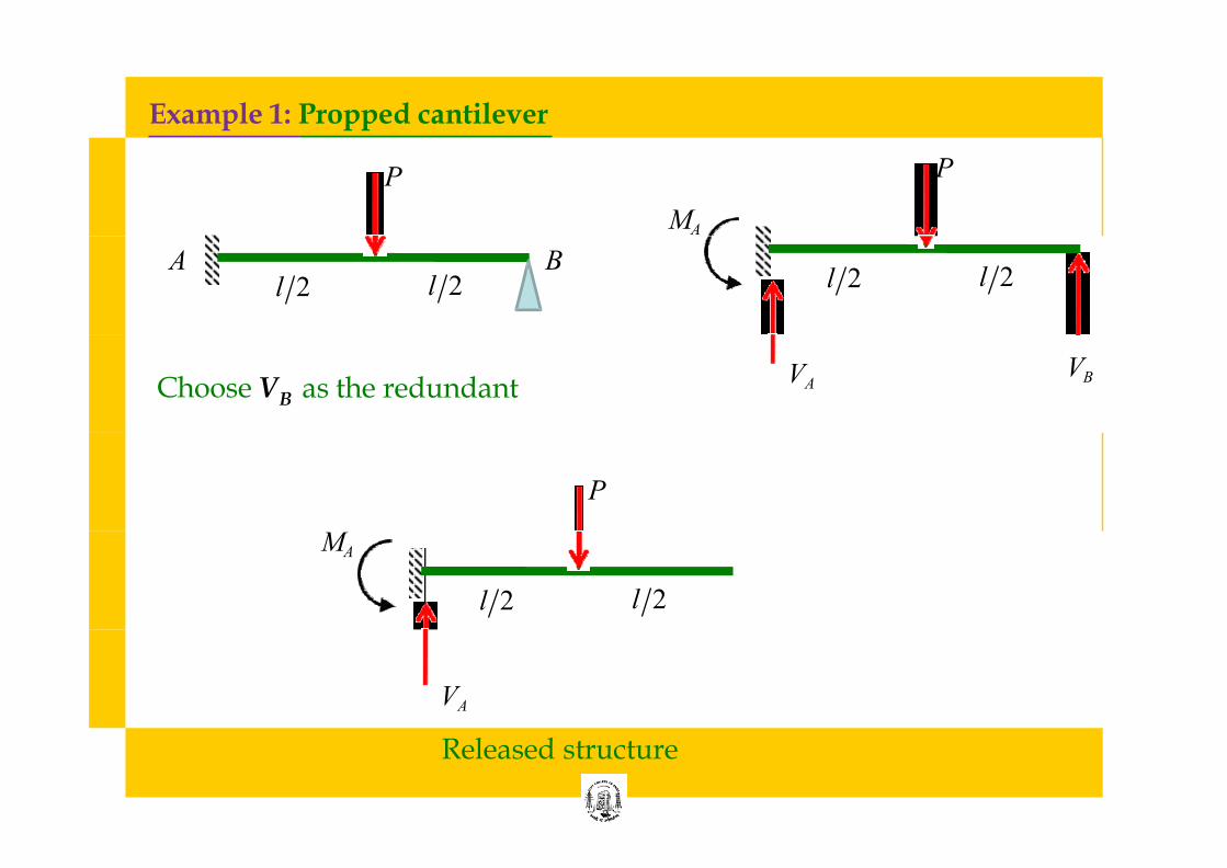
Example 1: Propped cantilever

MA

P P

l 2 l 2 l 2 l 2 A B

VA VB

Choose V B as the redundant

P

MA

l 2 l 2

VA

Released structure

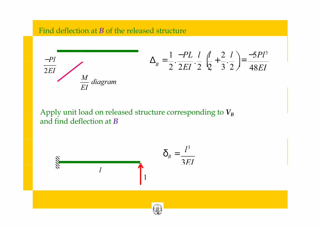
Find deflection at B of the released structure

2 l ⎞ −5Pl 3 1 −PL l ⎛ l Δ = . + . = −Pl .

2 2EI 2 ⎜ 2 3 2 ⎜ 48EI B ⎝ ⎠ 2EI

M diagram

EI

Apply unit load on released structure corresponding to VB

and find deflection at B

l 3

δ B = 3EI

l 1

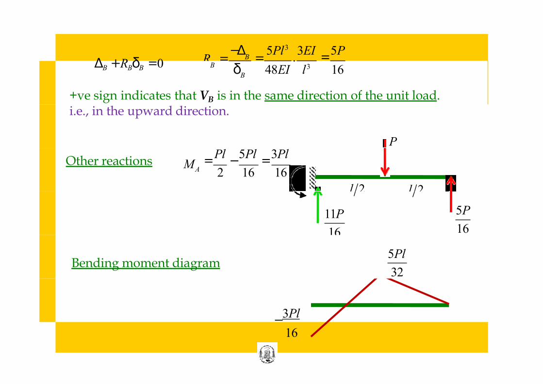
−Δ 5Pl3 3EI 5P B R = = . =

δ 48EI l3 16 ΔB + RBδB = 0 B

B

+ve sign indicates that VB is in the same direction of the unit load. i.e., in the upward direction.

P

l 2 l 2

= Pl

− 5Pl

= 3Pl

2 16 16 A M Other reactions

5P

16

11P

16

5Pl

32 Bending moment diagram

− 3Pl

16

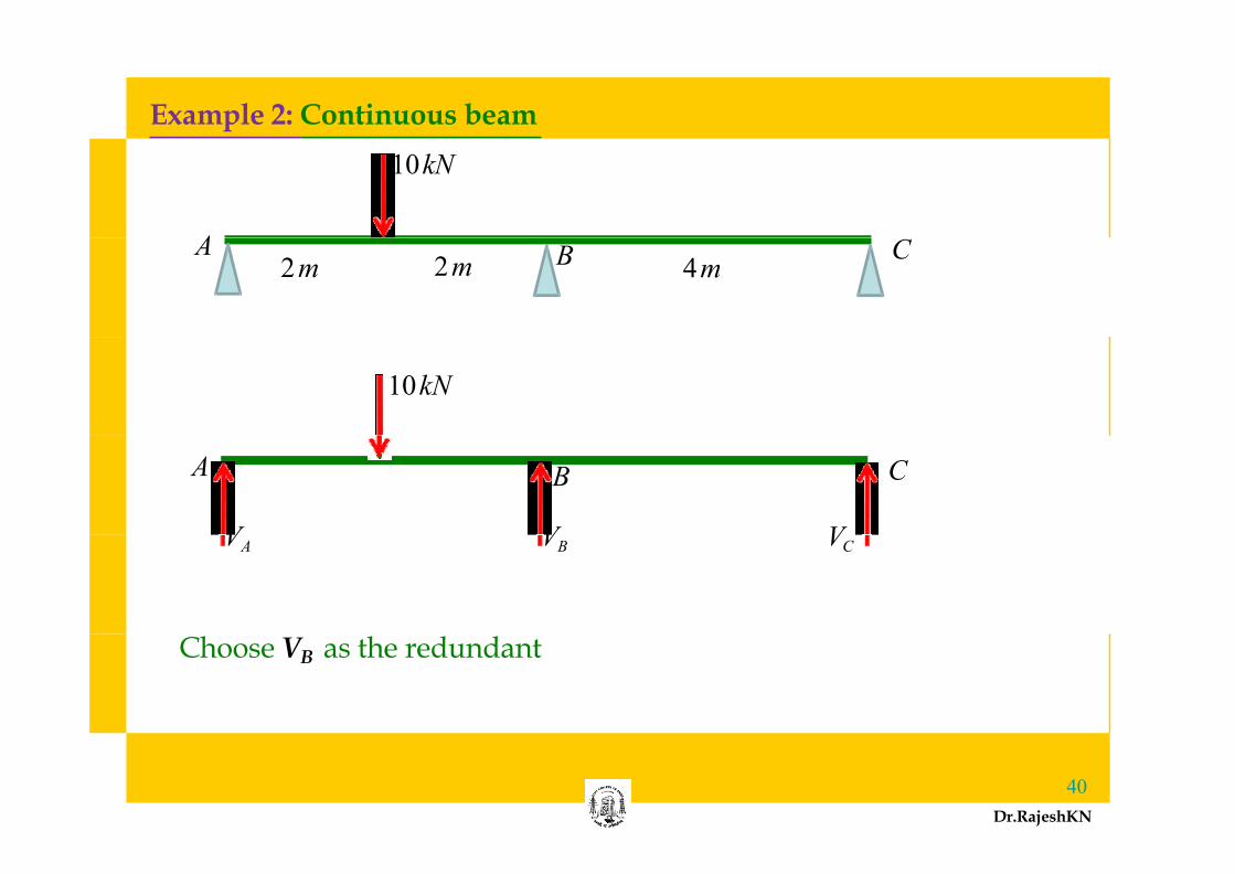
Example 2: Continuous beam

10 kN

2 m 2 m A B 4 m

C

10 kN

A B C

VA VC VB

Choose VB as the redundant

40

Dr.RajeshKN

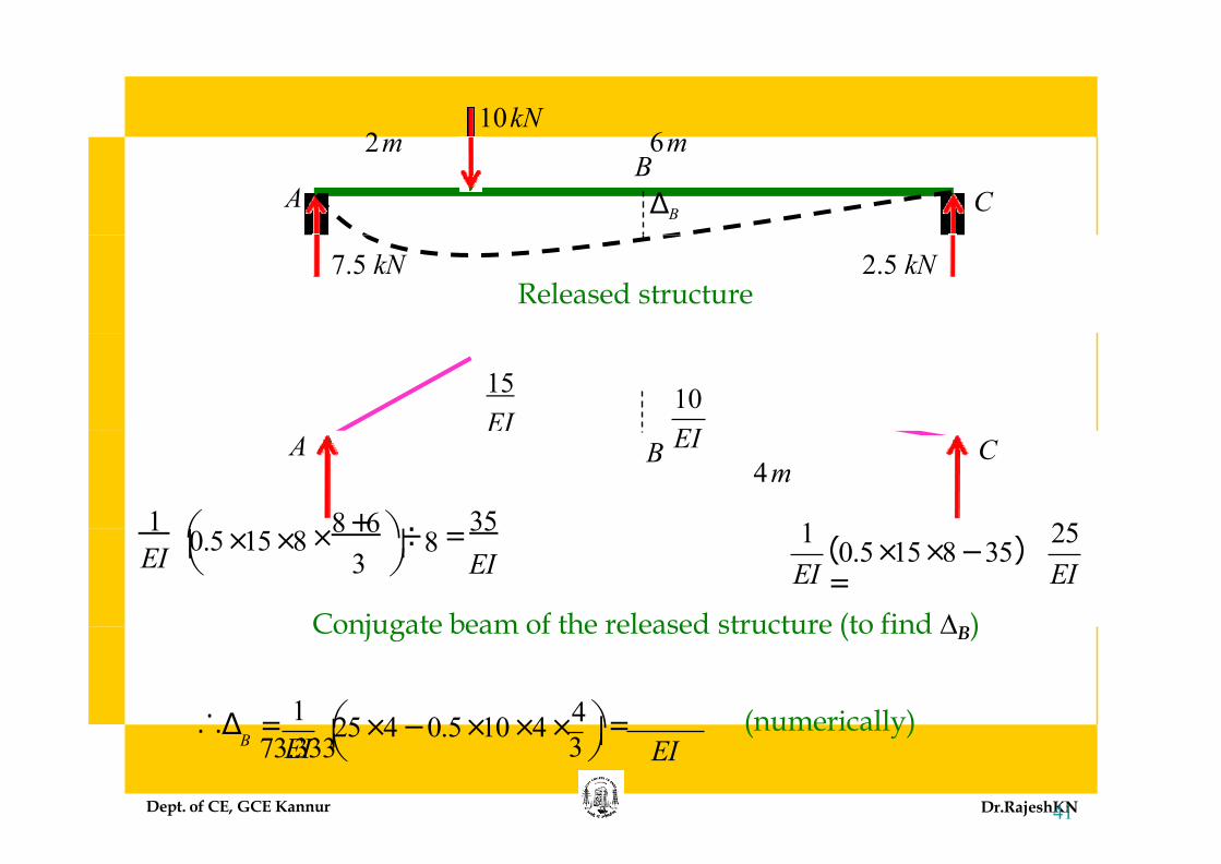
10 kN

A ΔB C

2 m 6 m B

Released structure 2.5 kN 7.5 kN

15

EI 10

1 ⎛ = 35

EI ×

8 + 6 ⎞ ÷

A B EI C

4 m

(0.5×15×8 − 35) =

1 25

EI EI 8

EI ⎜ 0.5×15×8

3 ⎠ ⎜

⎝

Conjugate beam of the released structure (to find ∆B)

= 1 ⎛ 25× 4 − 0.5×10 × 4 ×

4 ⎞ = 73.333

Dept. of CE, GCE Kannur Dr.RajeshK41N

3 ⎜ B EI

⎜ EI

∴Δ ⎝ ⎠

(numerically)

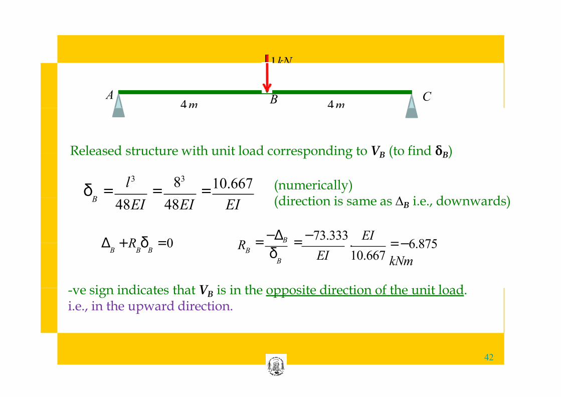
1kN

4 m A B 4 m

C

Released structure with unit load corresponding to VB (to find δB)

l3 83 10.667 δ = = = (numerically)

48EI 48EI B

EI

= −ΔB =

−73.333.

EI

(direction is same as ∆B i.e., downwards)

Δ + R δ = 0 B B B

= −6.875

kNm EI 10.667 B

B

R δ

-ve sign indicates that VB is in the opposite direction of the unit load. i.e., in the upward direction.

42

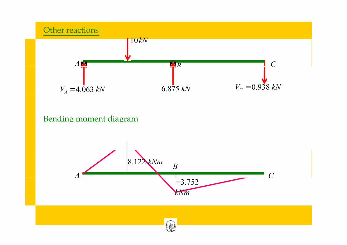
Other reactions 10 kN

A B C

VA = 4.063 kN VC = 0.938 kN 6.875 kN

Bending moment diagram

A B

C

8.122 kNm

−3.752

kNm

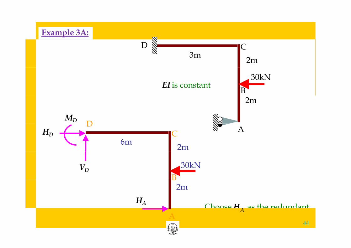
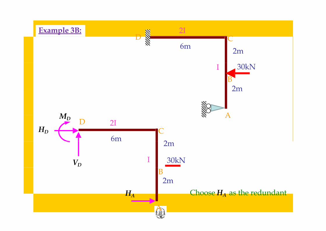
Example 3A:

C

2m 3m

D

30kN

B EI is constant

2m

MD

A

2m 6m

C D

HD

30kN

B 2m

VD

HA Choose H as the redundant

44 A

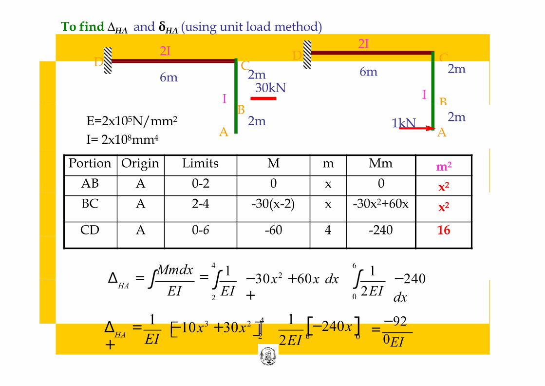
A

C D

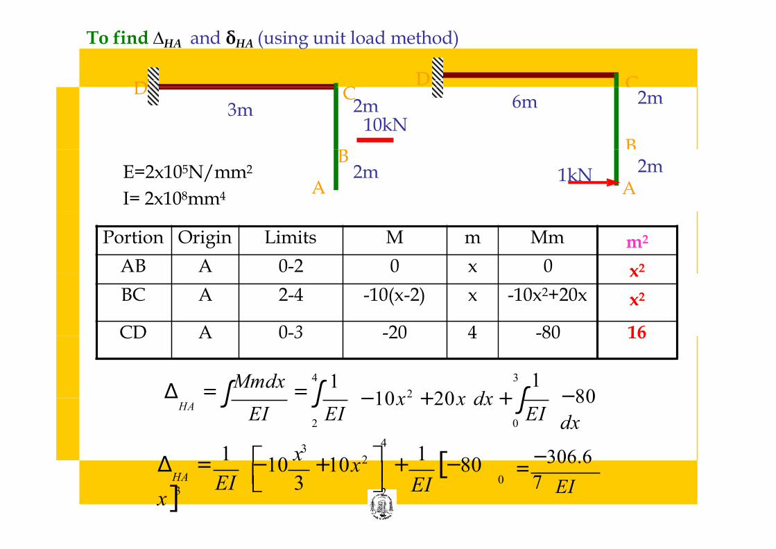
To find ∆HA and δHA (using unit load method)

2m 10kN

3m C D

2m 6m

B

2m A

B 2m

A 1kN E=2x105N/mm2

I= 2x108mm4

4 3 1 −10 x2 + 20 x dx + ∫ Δ = ∫

Mmdx = ∫

1

2 0

−80

dx HA

EI EI EI

4 3

Δ = 1 ⎡

−10 x

+ 10 x2 ⎤ + 1 [−80

x]3

−306.6

7 0 ⎦2 EI ⎜ 3 HA

EI ⎜

⎣ EI =

Portion Origin Limits M m Mm m2

AB A 0-2 0 x 0 x2

BC A 2-4 -10(x-2) x -10x2+20x x2

CD A 0-3 -20 4 -80 16

0 0 EI

4 3

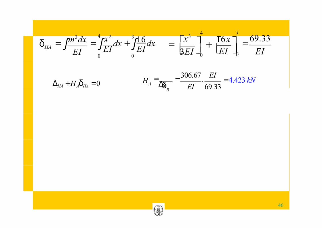
⎤ ⎡16x ⎤ 4 3 16 m2 dx x2

δ HA = ∫ = ∫ EI

dx + ∫ EI dx

⎡ x3

0 0

69.33 = ⎜⎣ 3EI ⎜⎦ EI

+ ⎜⎣ EI ⎜⎦ =

ΔHA + HAδHA = 0 =

306.67 .

EI = 4.423 kN

EI 69.33 = −ΔB

A H

δ B

46

Example 3B: 2I

2m 6m

C D

30kN I

B 2m

6m

2I C

D HD

MD A

30kN

2m

I VD

Choose HA as the redundant

B 2m

A

HA

2I 2I

C D

To find ∆HA and δHA (using unit load method)

2m 30kN

6m

I

C D 2m 6m

I B

2m A

B 2m

A 1kN E=2x105N/mm2

I= 2x108mm4

4

∫ 6

−30 x2 + 60 x dx

+

1 1 Mmdx =

2 0 2EI −240

dx HA

EI EI Δ = ∫ ∫

Δ = 1 ⎡−10x3 + 30x2 ⎤

4

+ [−240x]6

1 −92

0 0 ⎦2 2EI HA EI ⎣ EI

=

Portion Origin Limits M m Mm m2

AB A 0-2 0 x 0 x2

BC A 2-4 -30(x-2) x -30x2+60x x2

CD A 0-6 -60 4 -240 16

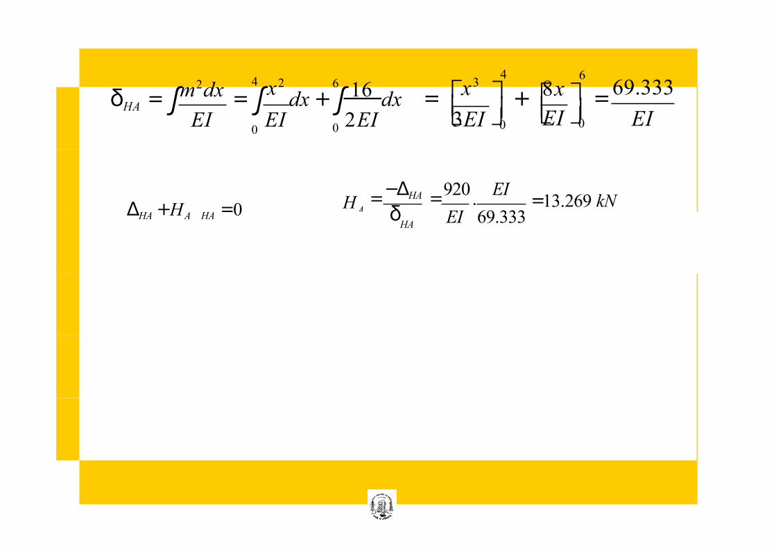
4 6 16 m2 dx x2

= ∫ dx + ∫ dx

0 0 2EI EI EI

4

⎤ 6

⎡ 8x ⎤ ⎡ x3

δ HA = ∫ ⎣ EI ⎦0 ⎣ 3EI ⎦0

69.333

EI = ⎜ + ⎜ = ⎜ ⎜

= −ΔHA =

920 .

EI = 13.269 kN

A H ΔHA + HA HA = 0 EI 69.333

HA δ

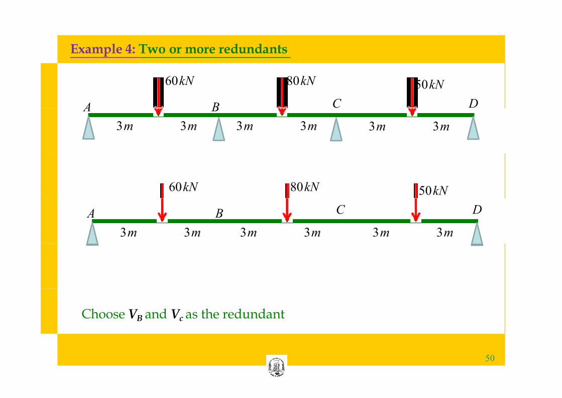
Example 4: Two or more redundants

60 kN 80 kN

A B

3m 3m 3m 3m

C

50 kN

D

3m 3m

60 kN 80 kN 50 kN

3m 3m

A B C D

3m 3m 3m 3m

Choose VB and Vc as the redundant

50

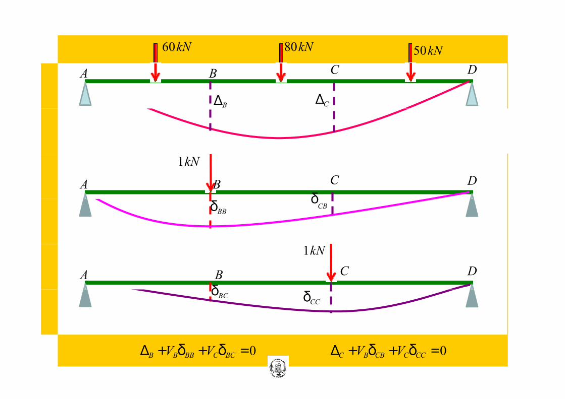
60 kN 80 kN 50 kN

A B C D

ΔB ΔC

1kN

A B D C

δBB CB

δ

1kN

A B D C

δBC δCC

ΔB +VBδBB +VCδBC = 0 ΔC +VBδCB +VCδCC = 0

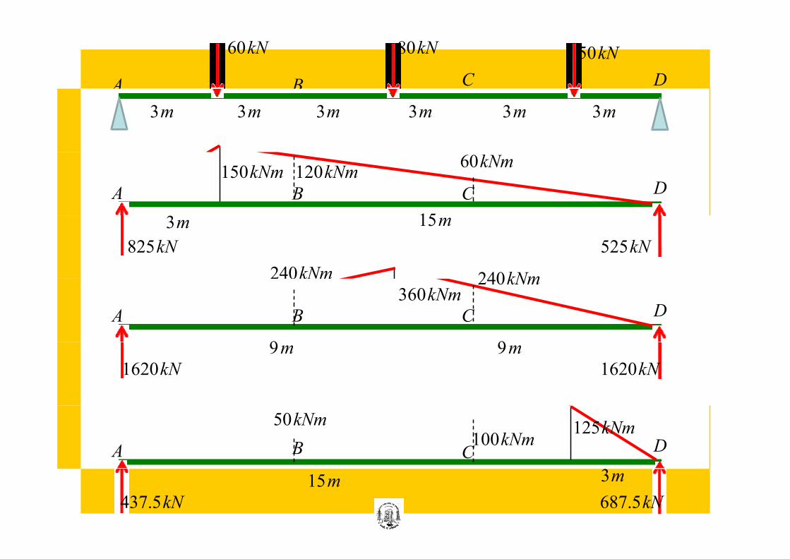
60 kN

A B C

80 kN 50 kN

D

3m 3m 3m 3m 3m 3m

A

150 kNm 120 kNm

B

60 kNm

C D

3m 15m

525kN 825kN

240 kNm

A B C D 360 kNm

240 kNm

9 m 9 m

1620 kN 1620 kN

A

50 kNm

B 100 kNm

C D 125kNm

15m 3m

687.5kN 437.5kN

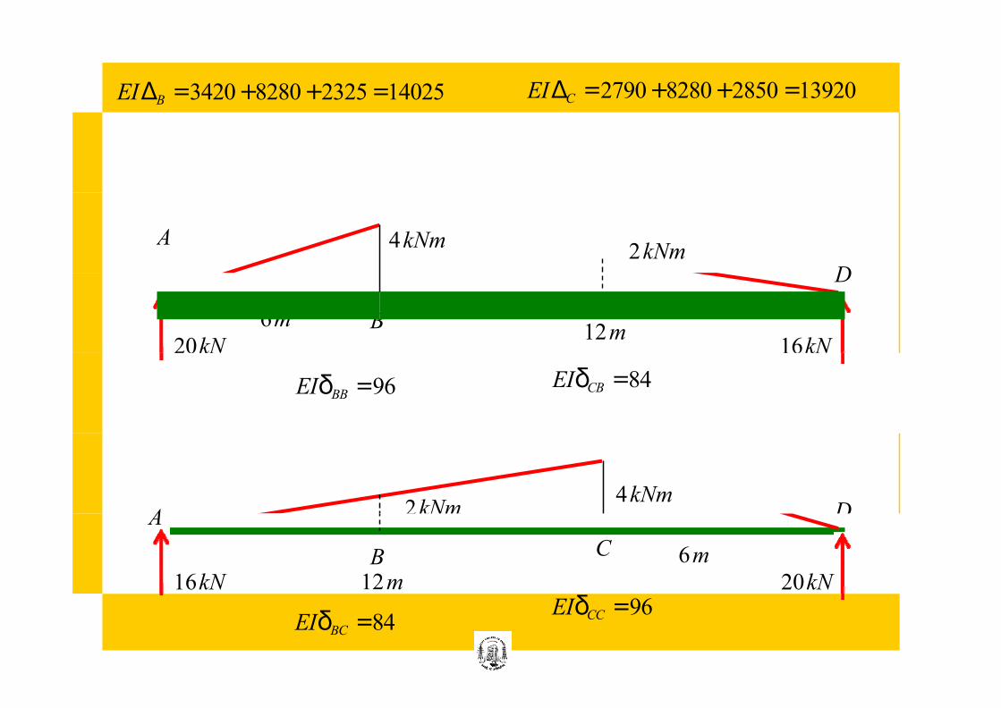
EIΔB = 3420 + 8280 + 2325 = 14025 EIΔC = 2790 + 8280 + 2850 = 13920

B C 12 m

D

6 m

16 kN 20 kN

EIδBB = 96 EIδCB = 84

D 2 kNm 4 kNm

A

B 12 m

C 6 m

20 kN 16 kN

EIδBC = 84 EIδCC = 96

A 4 kNm 2 kNm

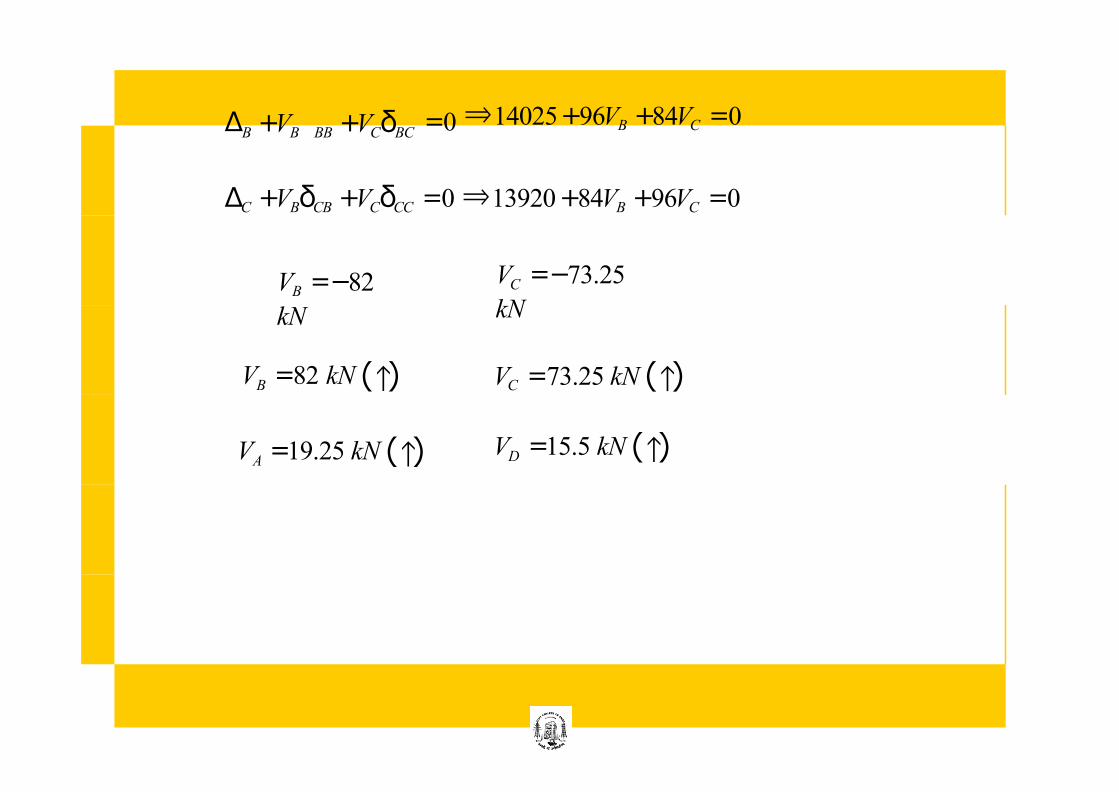
= 0 ⇒14025 + 96VB + 84VC = 0 B +VB BB +VCδBC Δ

ΔC +VBδCB +VCδCC = 0 ⇒13920 + 84VB + 96VC = 0

VB = −82

kN

VC = −73.25

kN

VB = 82 kN (↑) VC = 73.25 kN (↑)

VA = 19.25 kN (↑) VD = 15.5 kN (↑)

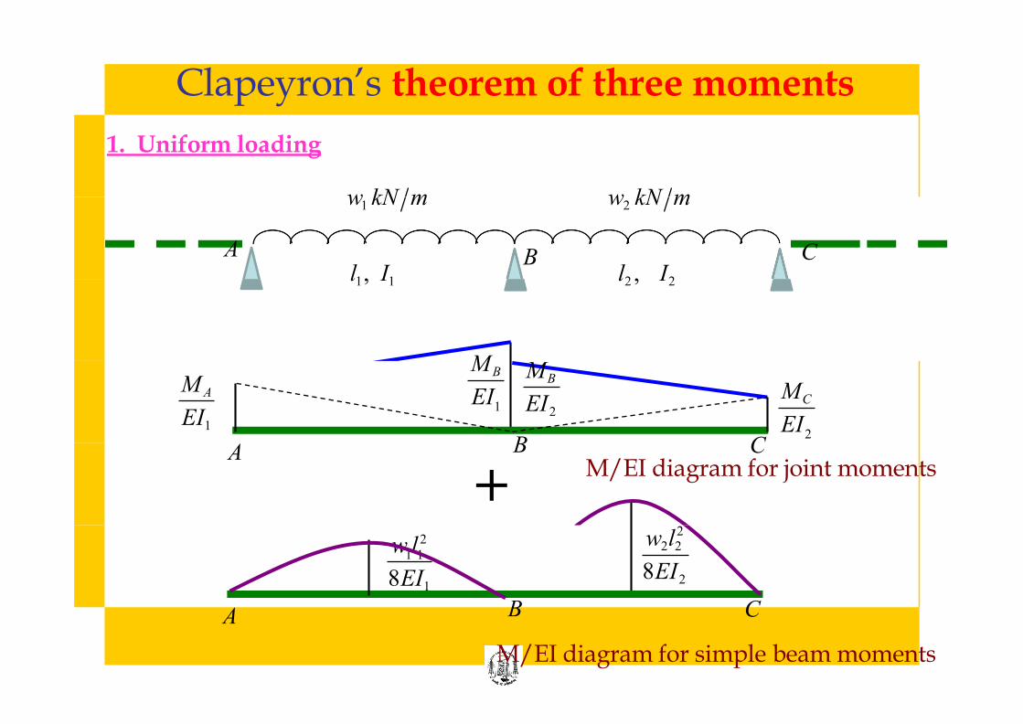
Clapeyron’s theorem of three moments

1. Uniform loading

w1 kN m

l1 , I1

A B C

w2 kN m

l2 , I2

EI1

M A 1

M B

EI EI2

M B

2

MC

EI

A B C M/EI diagram for joint moments

+ w l 2

1 1

8EI1

2 w2l2

8EI2

A B C

M/EI diagram for simple beam moments

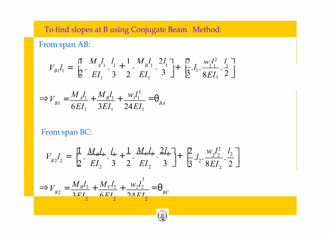
To find slopes at B using Conjugate Beam Method:

From span AB:

⎡ 2 w l 2 l ⎤ ⎡ 1 M l l 1 M l 2l ⎤ A 1 . 1 B 1 . 1 . . 1 1 . 1

3 ⎜ + ⎜ 3

l1 VB1l1 = ⎜ 2 1 1 1 ⎦

. + . EI 3 2 EI 8EI 2 ⎜ ⎣ ⎦ ⎣

M l M l w l 3 A 1 B 1 1 1

B1 6EI1 3EI1 24EI1

BA ⇒ V = = θ + +

From span BC:

⎡ 2 w l 2 l ⎤ B 2 . 2 C 2 . 2

⎜ + ⎜ 2 2 2

⎜ 2 B 2 2

2 2 2

⎡ 1 1 M l 2l ⎤ . + . .l . .

2 EI 3 2 EI 3 3 8EI 2

M l l V l = ⎜

⎣ ⎦ ⎣ ⎦

3

M Bl2 M C l2 w l 2 2 B 2

3EI 6EI 24EI BC

⇒ V = = θ + + 2 2 2

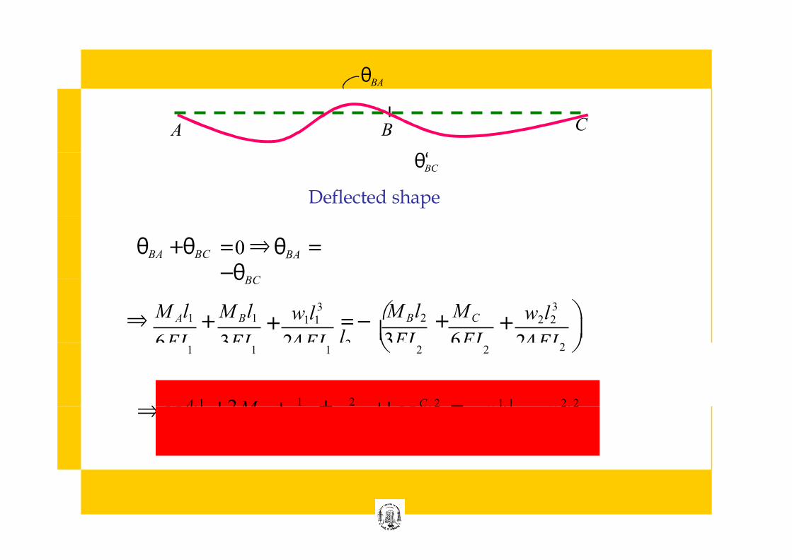
θBA

A B C

θBC

Deflected shape

= 0 ⇒ θBA =

−θBC

θBA + θBC

3 3

= − ⎛ M Bl2 +

M C

l2

w2l2 ⇒ M Al1 +

M Bl1 w1l1

⎜ 3EI 6EI 24EI 6EI 3EI 24EI

⎞ + + ⎜

2 2 2 ⎠ 1 1 1 ⎝

M l ⎛ l l ⎞ M l w l 3 w l 3 A 1 2 1 2 C 2 1 1 2 2

EI + M B ⎜ EI

+ EI ⎜ +

EI = –

EI –

EI 1 ⎝ 1 2 ⎠ 2 4 1 4 2

⇒

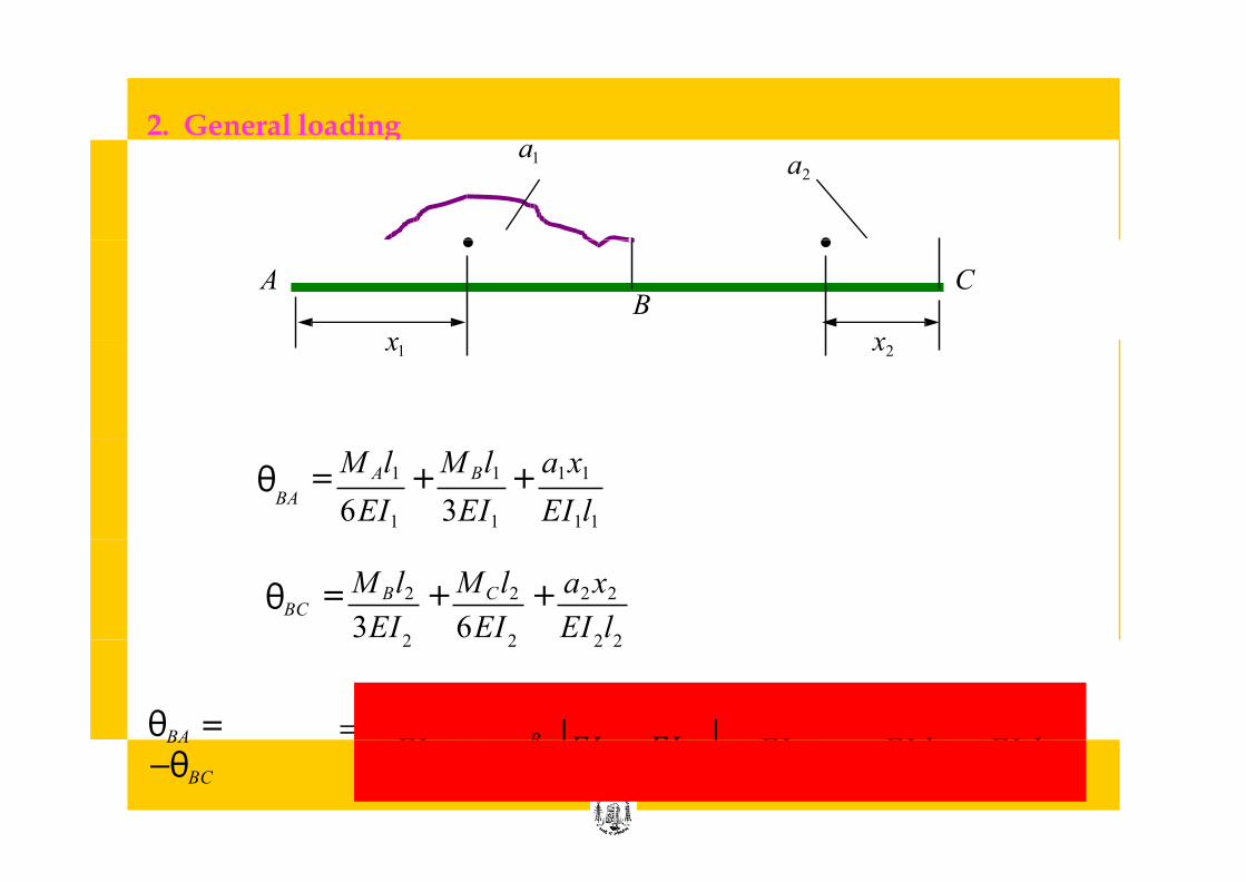
2. General loading a1 a2

A B

C

x1 x2

= M Al1 +

M Bl1 + a1 x1

6EI1 3EI1 EI1l1

BA θ

M Bl2 M C l2 a2 x2 = + + 3EI 6EI EI l

θBC

2 2 2 2

⇒ M Al1 + 2M

⎛ l1 + l2 ⎞

+ M C l2 = –

6a1 x1 – 6a2 x2

EI B ⎜ EI EI ⎜ EI EI l EI l 1 ⎝ 1 2 ⎠ 2 1 1 2 2

θBA =

−θBC

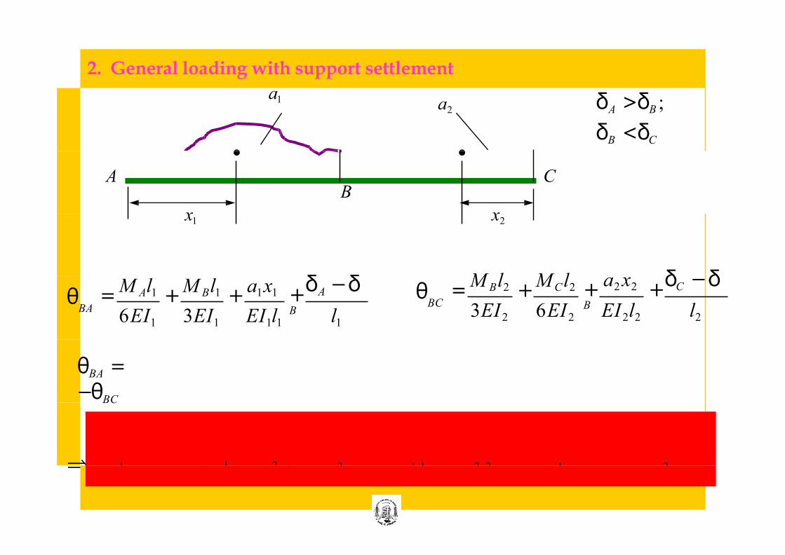
2. General loading with support settlement

a1 a2 δ A > δ B ;

δ B < δC

A B

C

x1 x2

= M Al1 +

M Bl1 + a1 x1

6EI1 3EI1 EI1l1 l1

+ δ A − δ

B BA θ =

M Bl2 + M C l2 +

a2 x2 + δC − δ

B 3EI2 6EI2 EI2l2 l2

BC θ

θBA =

−θBC

⇒

M Al1 + 2M ⎛ l1 +

l2 ⎞ +

MCl2 = – 6a1x1 –

6a2 x2 – 6(δ A – δB ) –

6(δC – δB ) EI B ⎜ EI EI ⎜ EI EI l EI l l l

⎝ ⎠ 1 1 2 2 1 1 2 2 1 2

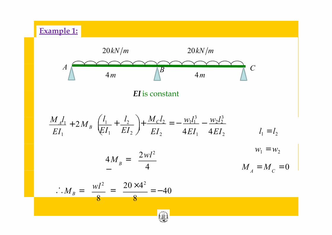
Example 1:

20 kN m 20 kN m

4 m A B C

4 m

EI is constant

l1 = l2

w l 3 w l 3 1 2 A 1

EI1

+ C 2 = − 1 1 − 2 2

⎝ EI1 EI2 ⎠ EI2 4EI1 4EI2

+ 2M B ⎜ l l M l ⎞ M l ⎛

+ ⎜

w1 = w2 2wl 2

4M = − 4

B M = M = 0

A C

wl 2

∴ M B = −

20 × 42

= −40

kNm

= − 8 8

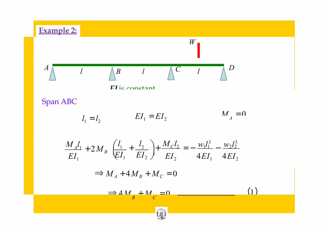
Example 2:

W

l A

B l

EI is constant

C l D

Span ABC

M = 0

w l 3 w l 3

l1 = l2 EI1 = EI2 A

1 2 A 1

EI1

+ C 2 = − 1 1 − 2 2

⎝ EI1 EI2 ⎠ EI2 4EI1 4EI2

+ 2M B ⎜ l l M l ⎞ M l ⎛

+ ⎜

⇒ M A + 4M B + M C = 0

⇒ 4M + M = 0 (1) B C

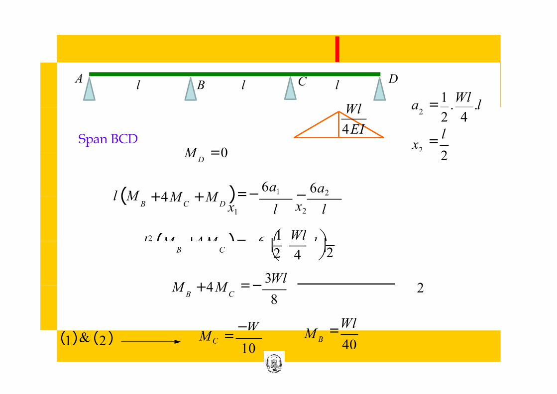
a = 1

.Wl

.l

l A

B C l l D

Span BCD 4EI

Wl 2

2

2 4

= l

2 x

) = − 6a1

x1

− 6a2

x2

M = 0 D

l 2 (M + 4M ) = −6 ⎛ 1 . Wl

.l ⎞

l

l (M + 4M + M B C D

l l

⎜ 2

⎜ 2 ⎝ 4

B C ⎠

= − 3Wl

M + 4M 8

B C 2

−W

l =

Wl

10 M C =

40 B

M ( ) & ( ) 1 2

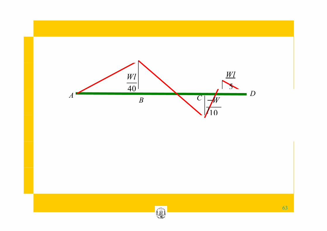
Wl Wl

5 A

B C

40

10

Bending moment diagram

−W

l

D

63

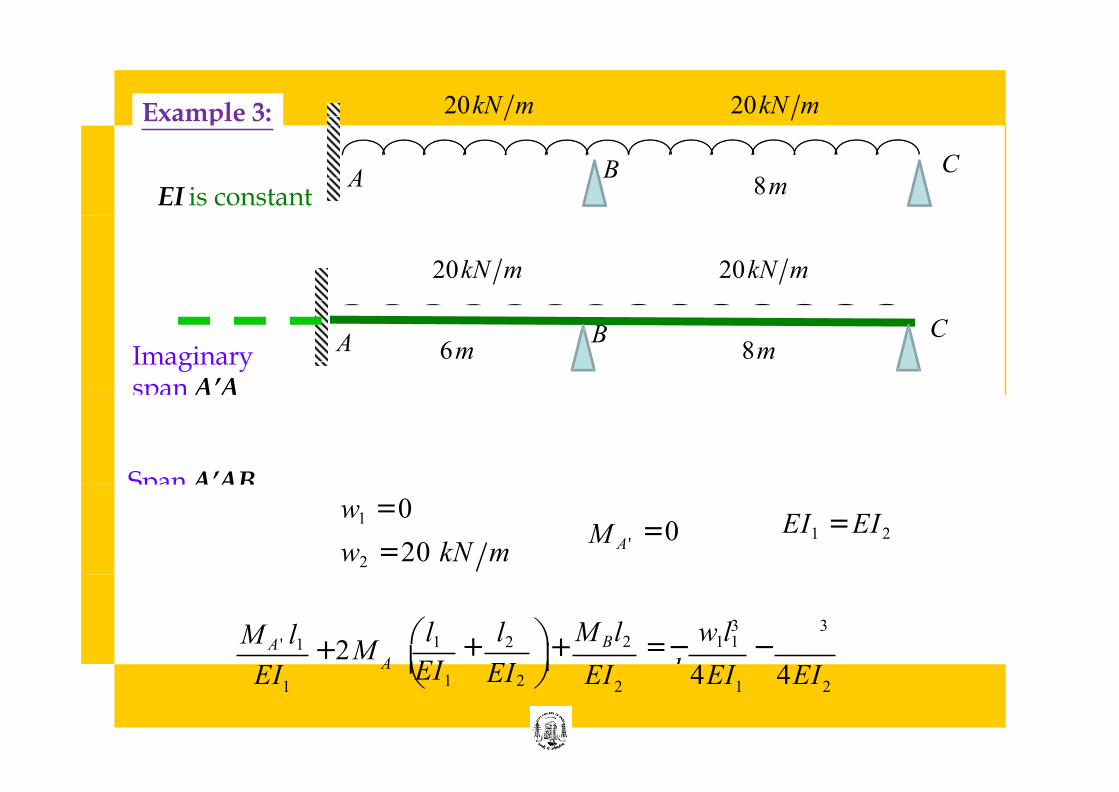
Example 3: 20 kN m 20 kN m

6 m A B C 8 m EI is constant

20 kN m 20 kN m

6 m A B C 8 m Imaginary

span A’A

Span A’AB w1 = 0

w2 = 20 kN m M A '

= 0 EI1 = EI2

3 3 l1 l2 M A ' l1 ⎞ +

M B l2 = − w1l1 −

w2l2

+ 2M ⎛

+ A ⎜ EI ⎜ ⎝ 1 2 ⎠ 1 2 1 2

4EI 4EI EI EI EI

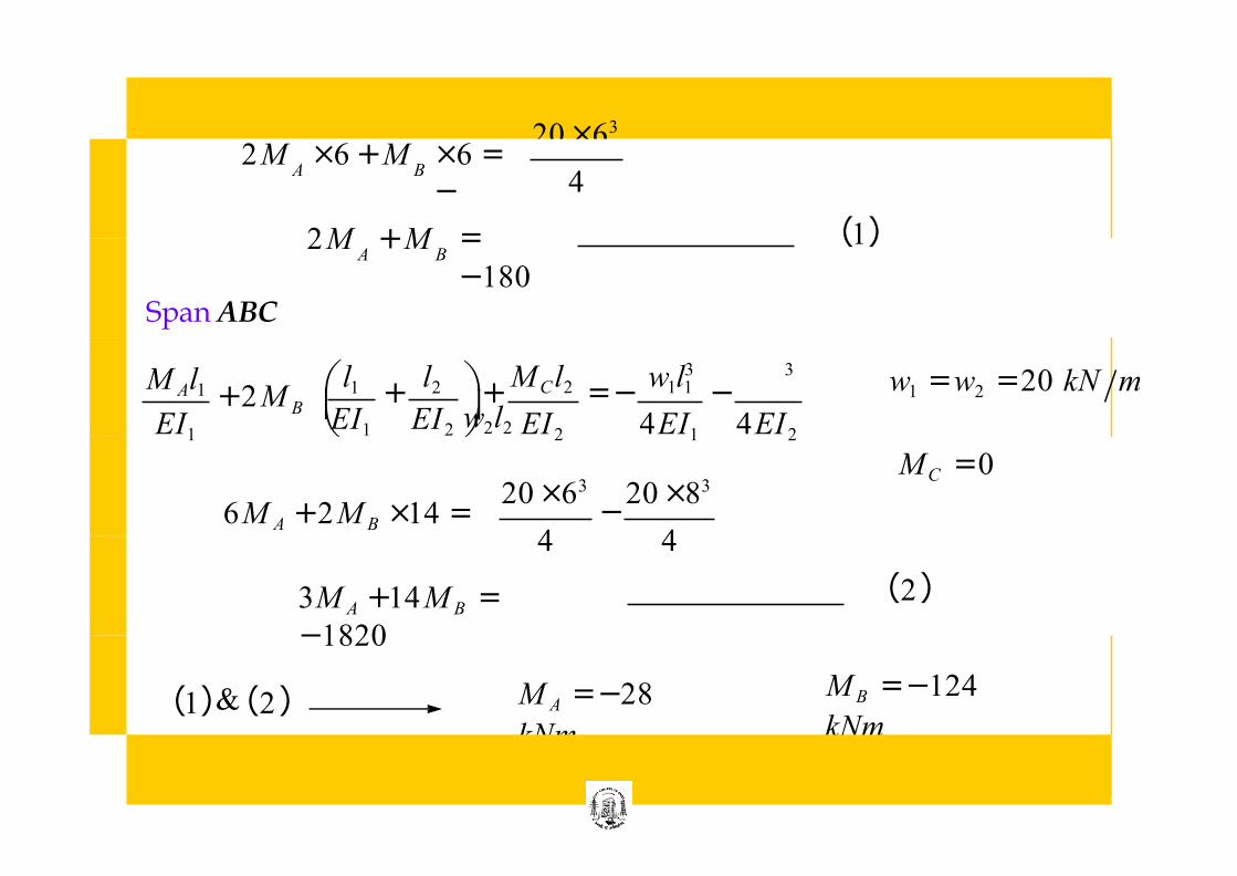
20 × 63

2M × 6 + M × 6 = − 4

A B

(1) 2M + M = −180

A B

Span ABC

w1 = w2 = 20 kN m 3 3 l1 l2 M Al1

⎞ +

M C l2 = − w1l1 −

w2l2 ⎝ EI1 EI2 ⎠ + 2M

EI2 4EI1 4EI2

B ⎜ EI1

⎛ + ⎜

M C = 0 20 × 63 20 × 83

6M A + 2M B ×14 = −

− 4 4

3M A + 14M B = −1820

(2)

(1) & (2) M A = −28

kNm

M B = −124

kNm

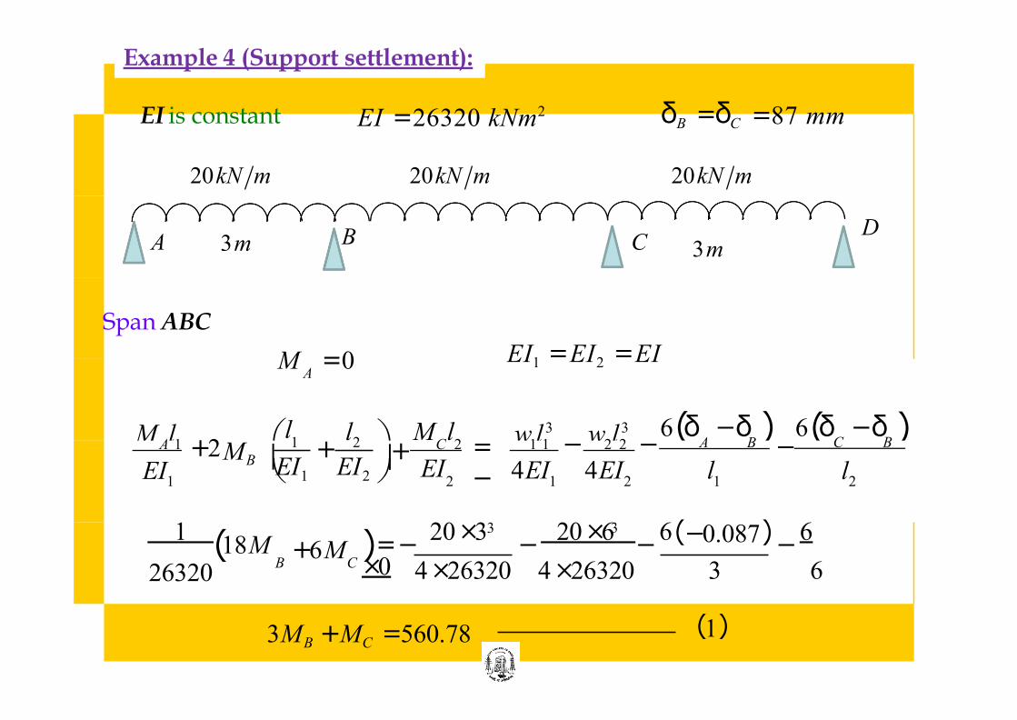
Example 4 (Support settlement):

EI = 26320 kNm2

20 kN m 20 kN m 20 kN m

= 87 mm δ B = δC EI is constant

6 m A D

C 3m B 3m

EI1 = EI2 = EI

Span ABC

M = 0 A

6(δ − δ ) 6(δ − δ ) w l3 w l3 ⎛ l l M l ⎞ M l 1 2 A 1 C 2 1 1 2 2

⎝ 1 2 ⎠ 1 2 1 2 1 2

+ 2 − − 4EI 4EI l

C B A B MB ⎜ EI

+ EI EI

⎜ + EI l

= −

−

1 (18M ) =− 20 ×3

− 20 ×6

− 6(−0.087)

− 6

×0

3 3

+ 6M 26320 4 × 26320 4 × 26320 3 6 B C

3MB + MC = 560.78 (1)

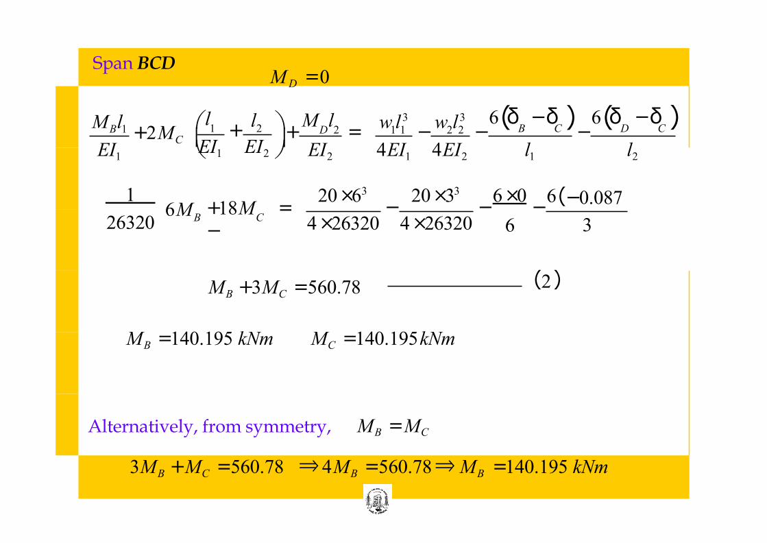
Span BCD M D = 0

6(δ − δ ) 6(δ − δ ) w l3 w l3 1 2 B 1 + 2M D 2 1 1 2 2 B C D C

C ⎜ ⎛ l l M l ⎞ M l

+ + = −

− − − ⎜ ⎝ EI1 EI2 ⎠ EI1 EI2 4EI1 4EI2 l1 l2

6(−0.087)

20 ×63 20 ×33 6 ×0

6

1

26320 6M +18M =

− 4 × 26320 4 × 26320 3 B C

− − −

MB + 3MC = 560.78 (2)

MB = 140.195 kNm MC = 140.195kNm

Alternatively, from symmetry, MB = MC

3MB + MC = 560.78 ⇒ 4MB = 560.78 ⇒ MB = 140.195 kNm

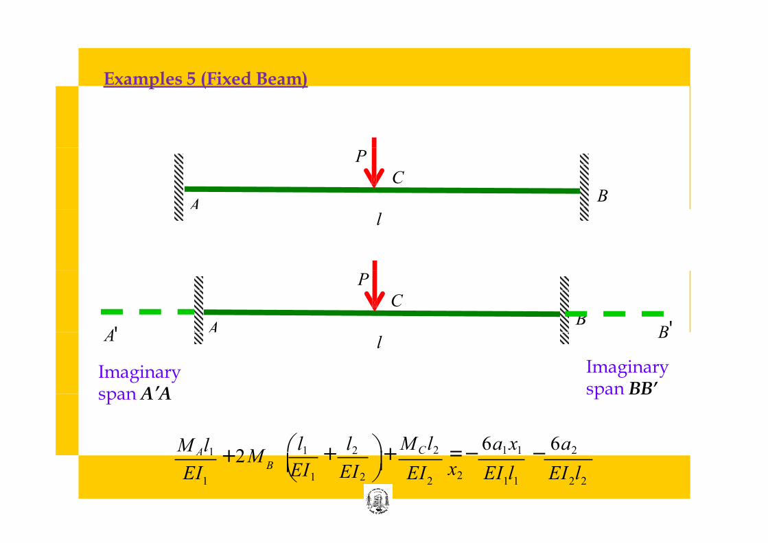
Examples 5 (Fixed Beam)

P

A B

C

l

P

A B

C

′ l A′ B

’ Imaginary span A A

Imaginary span BB’

l1 l2 M Al1 ⎞ +

M C l2 = − 6a1 x1 −

6a2

x2

⎛

⎝ 1 2 ⎠ 1 2 1 1 2 2

+ 2M B ⎜ EI EI EI EI EI l EI l

+ ⎜

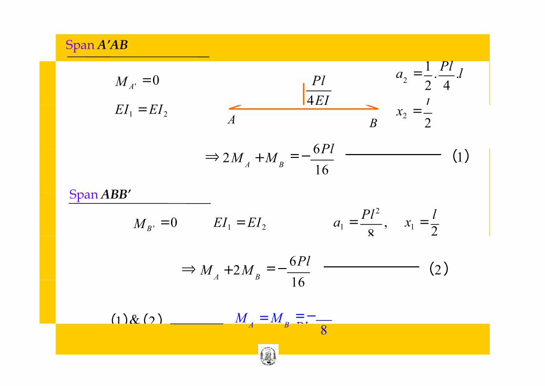
Span A’AB

M A ' = 0

4EI

Pl 2 a =

1 . Pl

.l 2 4

l EI1 = EI2 x2 = 2 A B

= − 6Pl

⇒ 2M + M 16

A B (1)

M B ' = 0 EI1 = EI2

Span ABB’

Pl 2

a1 = , x1 = 2 8

l

= − 6Pl

⇒ M + 2M A B

(2) 16

(1) & (2) = − Pl

M = M 8

A B

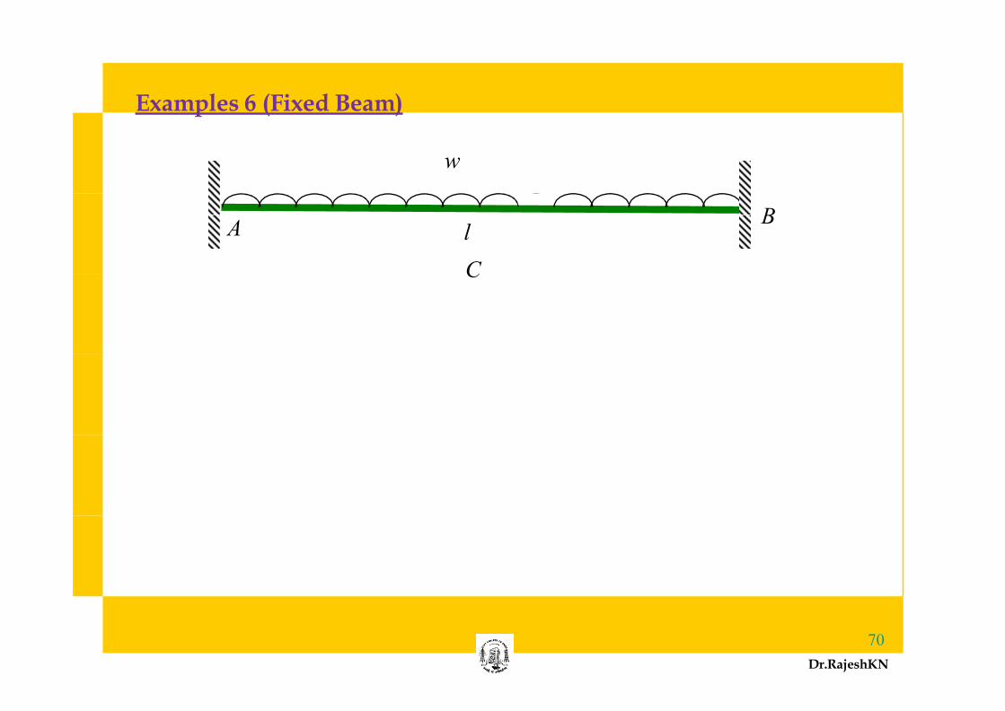
Examples 6 (Fixed Beam)

w

l

C

A B

70

Dr.RajeshKN

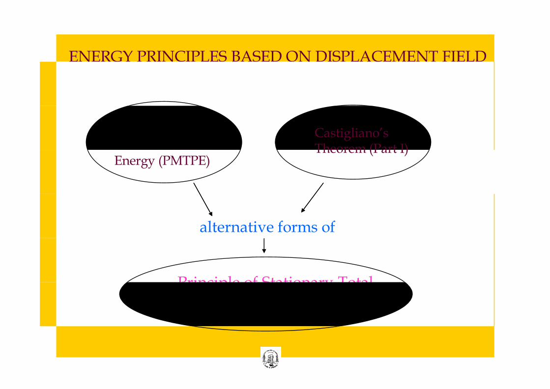
ENERGY PRINCIPLES BASED ON DISPLACEMENT FIELD

Principle of Minimum Total Potential

Castigliano’s Theorem (Part I)

Energy (PMTPE)

alternative forms of

Principle of Stationary Total Potential Energy (PSTPE)

Principle of Stationary Total Potential Energy (PSTPE)

When the displacement field in a loaded elastic structure is given a small and arbitrary perturbation, maintaining compatibility and without disturbing the associated force field, then the first variation of the total potential energy is equal to zero, if the forces are in a state of static equilibrium.

72

Alternative form of Principle of Stationary Total Potential Energy (PSTPE)

The total potential energy π in a loaded elastic structure expressed as a function of n independent displacements D1, D2, Dn … in a compatible displacement field must be rendered stationary, with the partial derivative of π with respect to every Dj being equal to zero, if the associated force field is to be in a state of static equilibrium.

Principle of Minimum Total Potential Energy (PMTPE)

When the displacement field in a loaded linear elastic structure is given a small and arbitrary perturbation, maintaining compatibility and without disturbing the associated force field, then the first variation of the total potential energy is equal to zero, if the forces are in a state of static equilibrium.

Castigliano’s Theorem (Part I)

If the strain energy, U, in an elastic structure, subject to a system of external forces in static equilibrium, can be expressed as a function of n independent displacements D1, D2, Dn … satisfying compatibility, then the partial derivative of U with respect to every Dj will be equal to the value of the conjugate force, Fj.

74

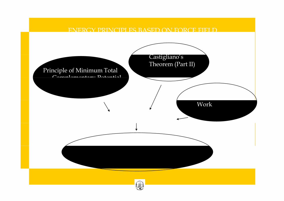
ENERGY PRINCIPLES BASED ON FORCE FIELD

Castigliano’s Theorem (Part II)

Principle of Minimum Total Complementary Potential Energy (PMTCPE)

Theorem of Least Work

alternative forms of

Principle of Complementary Energy (PSCTPE)

Stationary Total Potential

Principle of Stationary Total Complementary Potential Energy (PSTCPE)

When the force field in a loaded elastic structure is given a small and arbitrary perturbation, maintaining equilibrium compatibility and without disturbing the associated displacement field, then the first variation of the total complementary potential energy is equal to zero, if the displacements satisfy compatibility.

76

Alternative form of Principle Potential Energy (PSTCPE)

of Stationary Total Complementary

The total complementary potential energy π* in a loaded elastic structure expressed as a function of n independent forces F1, F2, … Fn in a statically admissible force field must be rendered stationary, with the partial derivative of π* with respect to every Fj being equal to zero, if the associated displacement field is to satisfy compatibility.

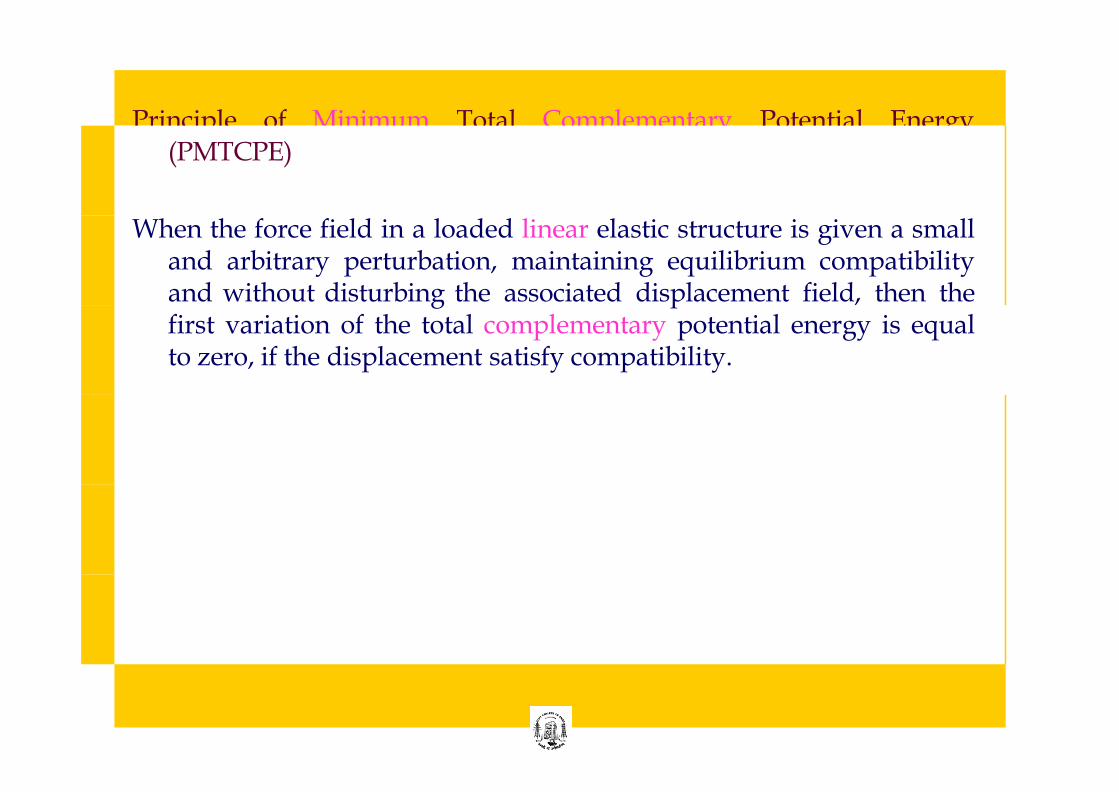
Principle of Minimum Total Complementary Potential Energy (PMTCPE)

When the force field in a loaded linear elastic structure is given a small and arbitrary perturbation, maintaining equilibrium compatibility and without disturbing the associated displacement field, then the first variation of the total complementary potential energy is equal to zero, if the displacement satisfy compatibility.

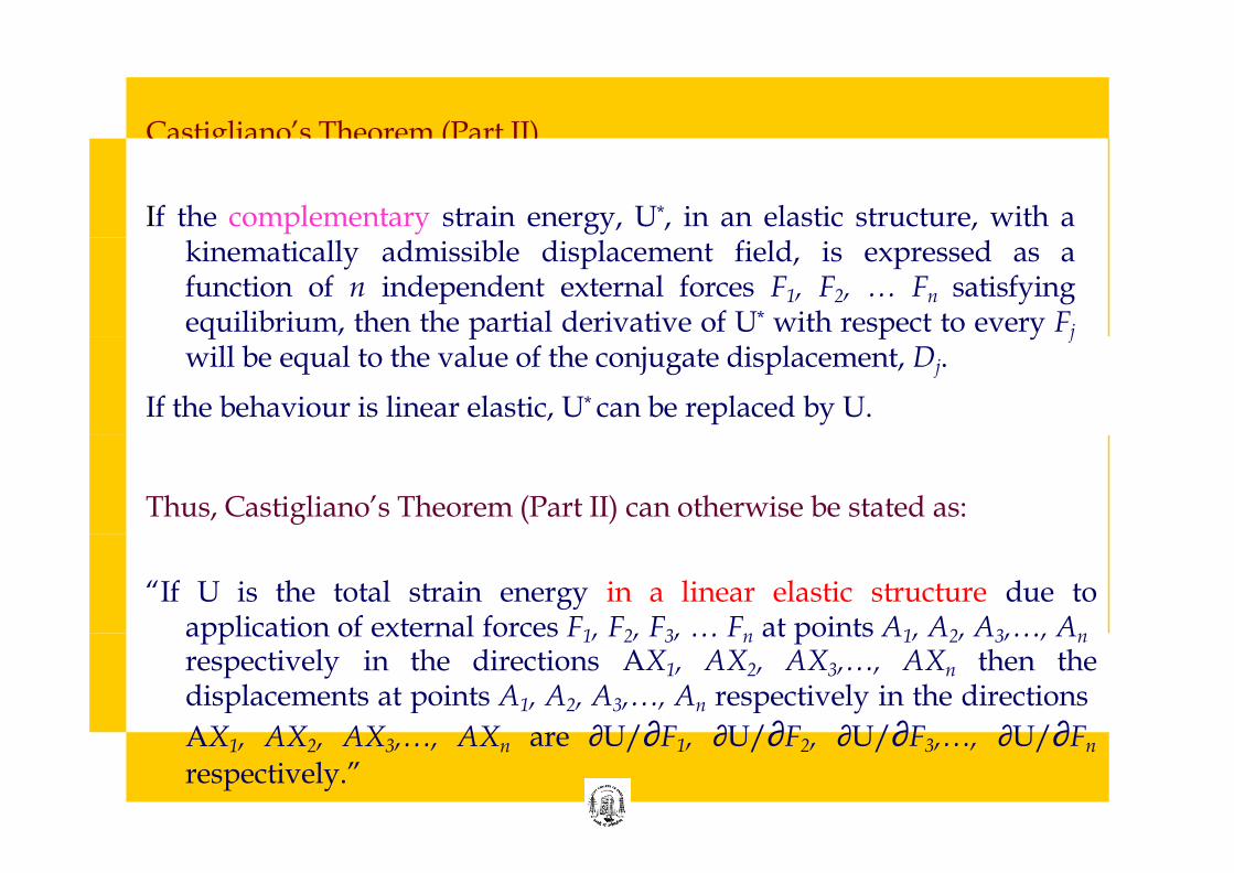
Castigliano’s Theorem (Part II)

If the complementary strain energy, U*, in an elastic structure, with a kinematically admissible displacement field, is expressed as a function of n independent external forces F1, F2, … Fn satisfying equilibrium, then the partial derivative of U* with respect to every Fj

will be equal to the value of the conjugate displacement, Dj.

If the behaviour is linear elastic, U* can be replaced by U.

Thus, Castigliano’s Theorem (Part II) can otherwise be stated as:

“If U is the total strain energy in a linear elastic structure due to application of external forces F1, F2, F3, … Fn at points A1, A2, A3,…, An

respectively in the directions AX1, AX2, AX3,…, AXn then the displacements at points A1, A2, A3,…, An respectively in the directions

AX1, AX2, AX3,…, AXn

respectively.” are ∂U/∂F1, ∂U/∂F2, ∂U/∂F3,…, ∂U/∂Fn

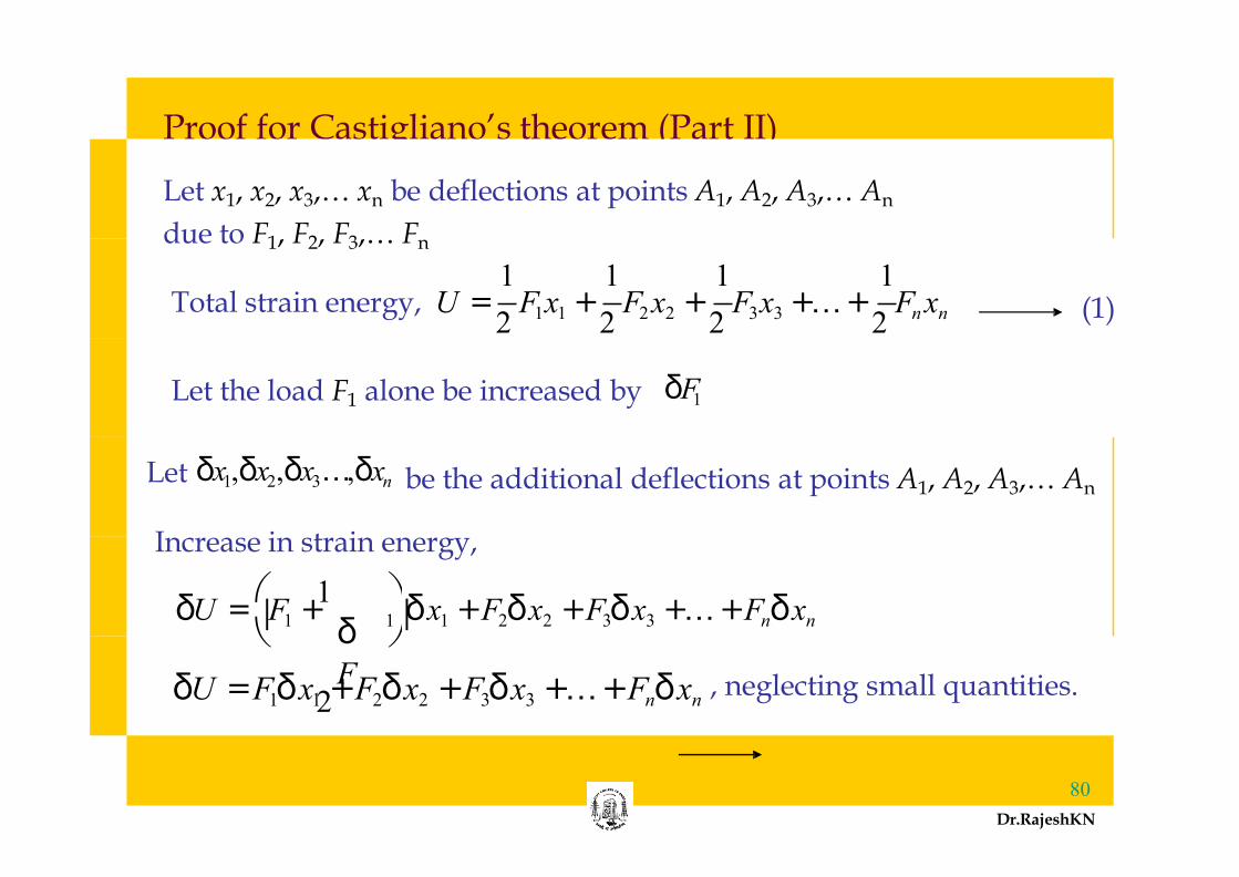
Proof for Castigliano’s theorem (Part II)

Let x1, x2, x3,… xn be deflections at points A1, A2, A3,… An

due to F1, F2, F3,… Fn

1 1 1 1 Total strain energy, U =

2 F1x1 +

2 F2 x2 +

2 F3 x3 + … +

2 Fn xn

Let the load F1 alone be increased by δF1

(1)

Let δx1,δx2,δx3…,δxn be the additional deflections at points A1, A2, A3,… An

Increase in strain energy,

δU = ⎜ F1 + 1 ⎜δ x1 + F2δ x2 + F3δ x3 + … + Fnδ xn

δU = F1δ x1 + F2δ x2 + F3δ x3 + … + Fnδ xn , neglecting small quantities.

(2) 80

Dr.RajeshKN

⎛ 1 ⎞

⎝ δ F

2

⎠

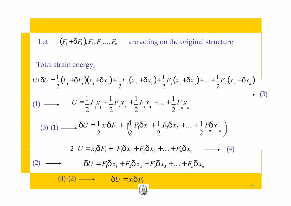
(F1 + δ F1 ), F2 , F3 …, Fn Let are acting on the original structure

U+δU = 1 (F + δ F ) ( x + δ x ) +

1 F ( x + δ x ) +

1 F ( x + δ x ) + … +

1 F ( x

Total strain energy,

+ δ x ) 1 1 1 1 2 2 2 3 3 3 n n

2 2 2 2 n

(3) U =

1 F x +

1 F x +

1 F x + … +

1 F x

2 1 1 2 2 2 2 3 3 2 n n (1)

1 ⎛ 1 1 1 ⎞ δU = x1δ F1 + ⎜ F1δ x1 + F2δ x2 + … + F δ x 2 2 2 2 n n ⎜

⎝

F1δ x1 + F2δ x2 + … + Fnδ xn

⎠ (3)-(1)

δU = F1δ x1 + F2δ x2 + F3δ x3 + … + Fnδ xn (2)

2 U = x1δ F1 + (4)

81 δU = x1δ F1

(4)-(2)

δU = x

δ F 1

1

When δ F1 → 0, ∂F

= x1

1

∂U

2 2 n ∂F2 ∂F3 ∂Fn

, x = ∂U

,… x = ∂U

= ∂U

Similarly, x

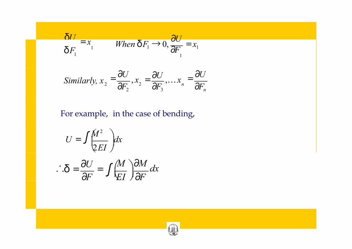
For example, in the case of bending,

⎛ M 2

∫ ⎝ 2EI ⎠

U = ⎜ dx ⎞

⎜

∴δ = ∂U

= ⎛ M ⎞ ∂M

dx ∂F ⎜ EI ⎜ ∂F

∫ ⎝ ⎠

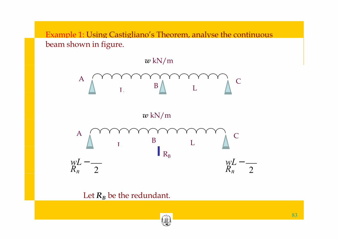
Example 1: Using Castigliano’s Theorem, analyse the continuous

w kN/m

beam shown in figure.

A B

C L L

w kN/m

A B

C L L

RB

2 wL − RB 2

wL − RB

Let RB be the redundant.

83

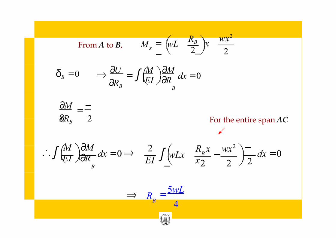
wx2

2 2 ⎜ B ⎞ x

− x

R M = ⎛ wL

− ⎜ ⎝ ⎠

From A to B,

δB = 0 dx = 0 ∂U ⎛ M ⎞ ∂M

∂RB

∫ ⎝ EI ⎠ ∂R B

⇒ = ⎜ ⎜

∂M =

−

x ∂RB 2 For the entire span AC

R x wx2 ⎞ −

x

2 dx = 0 ⇒ dx = 0

⎠ 2 2 2

B ∫ ⎝ EI ⎠ ∂R B

⎛ M ⎞ ∂M ⎜ wLx

− EI ∫ ⎝

⎛ ∴ − ⎜ ⎜ ⎜

= 5wL

⇒ R 4

B

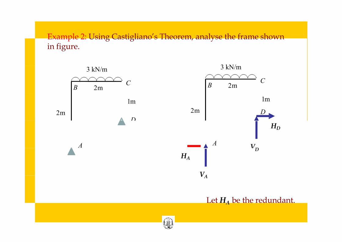
Example 2: Using Castigliano’s Theorem, analyse the frame shown in figure.

3 kN/m

2m B C

3 kN/m

2m B C

2m

1m

D

2m

1m

D

A A V

HD

D

VA

HA

Let HA be the redundant.

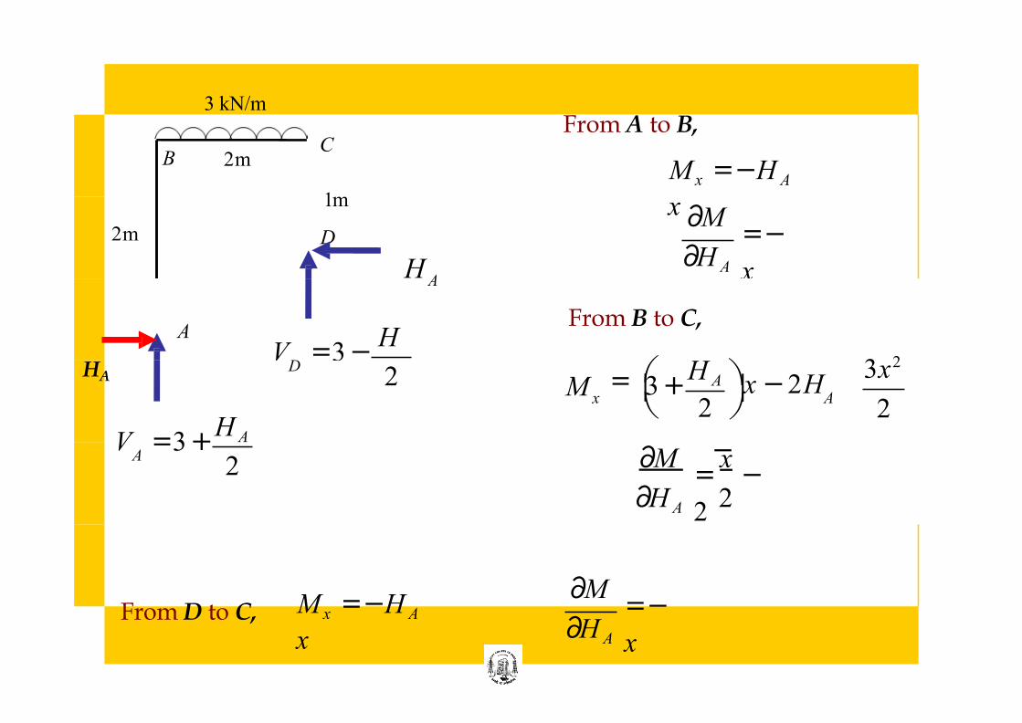
3 kN/m From A to B,

2m B C

M x = −H A

x 2m

1m

D

H ∂H A

∂M = −

x

A V = 3 −

H A

A

From B to C,

HA 2 D

V = 3 + H A

3x2 A ⎞ x − 2H

−

⎜ 3 + 2 2 ⎠ x A

H M = ⎛ ⎜

⎝

∂M x

∂H A 2

2 A

= −

2

∂M From D to C, M x = −H A

x ∂H A

= −

x

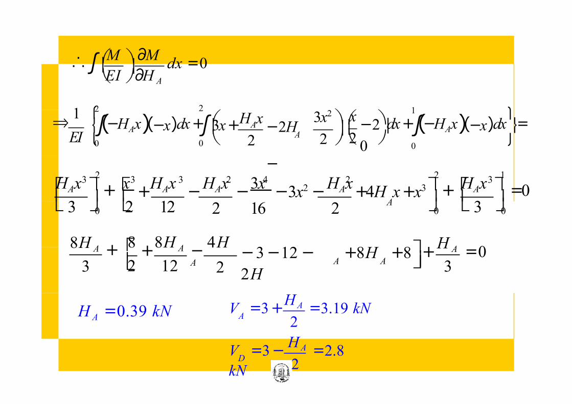
⎛ M ⎞ ∂M dx = 0

⎝ EI ⎠ ∂H A

∴ ∫ ⎜ ⎜

⇒ ⎨ (−HAx)(−x) dx + ⎜3x + −2⎜dx + (−HAx)(−x) dx⎬ =

0

1 ⎧2 2

⎛ 1

3x2 ⎞⎛ x ⎞

EI ⎩0 0 ⎝ ∫ 0

−2H

−

2 ⎠⎝ 2 ⎠ 2

A A

H x ⎫ ⎜⎜

⎭ ∫ ∫

2 2 1 3 3 3 2 4 2 3 ⎡ HAx ⎤ + ⎡ x

+ HAx

− HAx

− 3x

−3x2 − HAx

+ 4H x + x3⎤ + ⎡HAx ⎤ = 0 ⎜ ⎜ ⎜ ⎜ ⎜ ⎜ ⎣ 3 ⎦0 ⎣ 2 12 ⎦0 ⎣ 3 ⎦0 2 16 2

A

8H A + ⎡ 8 +

8H A − 4H

A + 8H + 8⎤ +

H A = 0 − 3 − 12 −

2H 3 3 ⎜⎣ 2 12 2

A A ⎜⎦

V = 3 + H A = 3.19 kN 2

A H A = 0.39 kN

V = 3 − H A = 2.8

kN 2 D

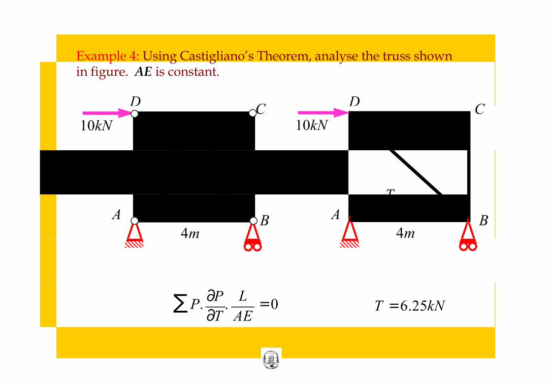
Example 4: Using Castigliano’s Theorem, analyse the truss shown in figure. AE is constant.

D D

10kN C

T 10kN C

3m

4m 4m

3m

T

A B A B

P. ∂P

. = 0 L

∂T AE ∑ T = 6.25kN

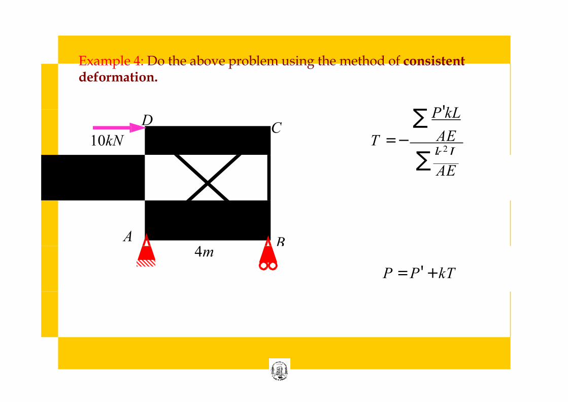
Example 4: Do the above problem using the method of consistent deformation.

10kN k 2 L

P′kL ∑ T = − AE

C D

3m

∑ AE

A B 4m

P = P′ + kT

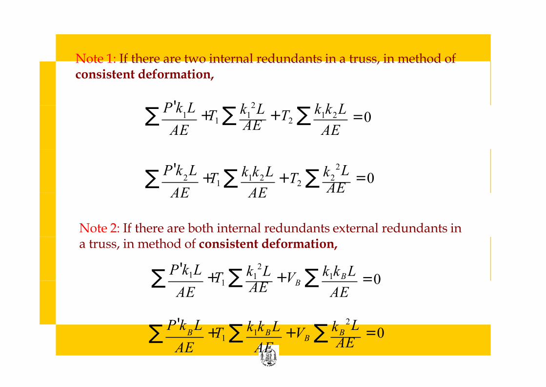
Note 1: If there are two internal redundants in a truss, in method of consistent deformation,

k 2 L 1 1 1 2 +T1 ∑ AE

+ T2 ∑ = 0 P′k L k k L

AE AE ∑

2 L 2 1 2 2 +T1 ∑ + T2 ∑ AE

= 0 P′k L k k L k ∑

AE AE

Note 2: If there are both internal redundants external redundants in a truss, in method of consistent deformation,

2 P′k1L k1 L k1kB L +T1 ∑ AE + VB ∑ = 0

AE AE ∑

2 L 1 B +T1 ∑ + VB ∑ AE

= 0 B B P′k L k k L k

AE AE ∑

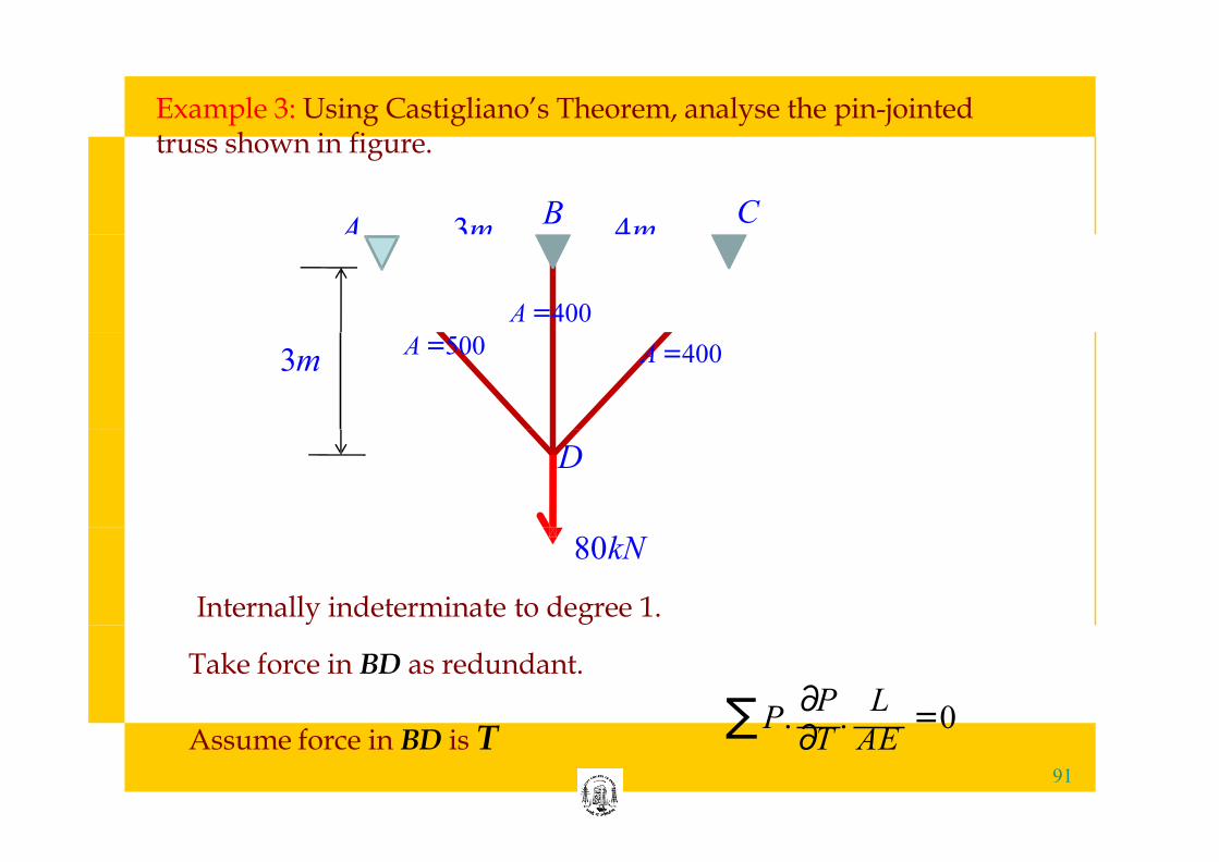
Example 3: Using Castigliano’s Theorem, analyse the pin-jointed truss shown in figure.

A 3m 4m B C

A = 400

3m A = 500 A = 400

D

80kN

Internally indeterminate to degree 1.

Take force in BD as redundant.

∂P L

91

Assume force in BD is T ∑ P. ∂T

. AE

= 0

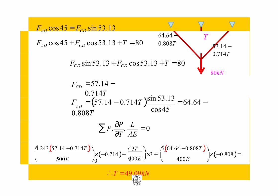
FAD cos 45 = FCD sin 53.13

FAD cos 45 + FCD cos 53.13 + T = 80 T

57.14 −

0.714T

64.64 −

0.808T

FCD sin 53.13 + FCD cos 53.13 + T = 80

80kN

= 57.14 −

0.714T

FCD

F = (57.14 − 0.714T ) sin 53.13 = 64.64 −

0.808T cos 45

AD

P. ∂P

. = 0 L

∂T AE ∑

⎛ 4.243(57.14 − 0.714T ) ⎞ ⎛ 3T ⎞ ⎛ 5 (64.64 − 0.808T ) ⎞ × (−0.714) + × 3 + × (−0.808) = 0 500E

⎜ 400E ⎜ 400E ⎜ ⎜ ⎜ ⎜

⎝ ⎠ ⎝ ⎠ ⎝ ⎠

∴ T = 49.09kN

Summary

Statically and kinematically indeterminate structures

• Degree of static indeterminacy, Degree of kinematic indeterminacy, Force and displacement method of analysis

Force method of analysis

•Method of consistent deformation-Analysis of fixed and continuous beams

•Clapeyron’s theorem of three moments-Analysis of fixed and continuous beams

•Principle of minimum strain energy-Castigliano’s second theorem- Analysis of beams, plane trusses and plane frames.