independent measurement of extinction and backscatter profiles in cirrus clouds by using a combined...

Independent measurement of extinction andbackscatter profiles in cirrus clouds by using acombined Raman elastic-backscatter lidar

Albert Ansmann, Ulla Wandinger, Maren Riebesell, Claus Weitkamp,and Walfried Michaelis

Height profiles of the extinction and the backscatter coefficients in cirrus clouds are determinedindependently from elastic- and inelastic- (Raman) backscatter signals. An extended error analysis isgiven. Examples covering the measured range of extinction-to-backscatter ratios (lidar ratios) in iceclouds are presented. Lidar ratios between 5 and 15 sr are usually found. A strong variation between 2and 20 sr can be observed within one cloud profile. Particle extinction coefficients determined frominelastic-backscatter signals and from elastic-backscatter signals by using the Klett method arecompared. The Klett solution of the extinction profile can be highly erroneous if the lidar ratio variesalong the measuring range. On the other hand, simple backscatter lidars can provide reliableinformation about the cloud optical depth and the mean cloud lidar ratio.

Key words: Combined lidar, Raman lidar, backscatter lidar, lidar ratio, particle extinction, particlebackscatter, Klett method, cirrus observation.

1. Introduction

High-altitude cirrus clouds have been identified asone important regulator of the radiance balance ofthe earth-atmosphere system.' In particular, opti-cally thin cirrus are of great interest since an increaseof the area covered by these clouds, which may beinduced partly by contrails, is expected to enhance thegreenhouse effect. In spite of the importance of iceclouds, measurements of their microphysical proper-ties (ice-crystal characteristics) and of their radiativeproperties (extinction, reflection, and emission) arerare' mainly because of their high location in theatmosphere. Extended studies of cirrus clouds wereperformed only recently in two regional experiments,the First International Satellite Cloud ClimatologyProject (ISCCP) Regional Experiment (FIRE)2 andthe International Cirrus Experiment (ICE).3 In bothinvestigations high-flying aircraft as well as ground-based observation stations were utilized.

In this paper, lidar measurements taken in cirrusclouds during ICE'89 in September and October 1989

The authors are with the Institut fr Physik, GKSS-Forschungs-zentrum Geesthacht GmbH, Postfach 1160, W-2054 Geesthacht,Germany.

Received 5 June 1991.0003-6935/92/337113-19$05.00/0.t 1992 Optical Society of America.

are presented. For what is, to our knowledge, thefirst time, profiles of the extinction and backscattercoefficients in high-level ice clouds are measuredindependently of each other with a combined Ramanelastic-backscatter lidar. In the technique applied,short laser pulses at a wavelength of 308 nm aretransmitted vertically into the atmosphere, and theheight profiles of signals elastically backscattered byair molecules and particles (at 308 nm) and inelasti-cally (Raman) backscattered by nitrogen molecules at332 nm (vibrational-rotational spectrum) are recorded.The particle extinction coefficient is determined fromthe inelastic-backscatter signal profile, while theparticle backscatter coefficient is derived from theratio of the elastic backscatter to the Raman signal, asis usual in the combined lidar technique.5 6

The independent measurement of the particle ex-tinction and backscatter coefficients and, thus, of theextinction-to-backscatter ratio, or lidar ratio, pro-vides information on the transmission and the reflec-tion properties of cirrus clouds and also on theice-crystal characteristics because the lidar ratio de-pends on shape, size, and orientation of the aniso-tropic ice particles. The influence of the microphysi-cal properties on the extinction-to-backscatter ratio isdiscussed here on the basis of measurement exam-ples.

The lidar ratio is one important input parameter

20 November 1992 / Vol. 31, No. 33 / APPLIED OPTICS 7113

for the determination of the particle extinction coeffi-cient from the elastic-backscatter signal alone.]- 0

In this technique, which originates from Hitschfeldand Bordan's radar application,"1 the particle extinc-tion or backscatter coefficient is obtained by solving aBernoulli equation that is derived from the basic lidarequation with the assumption of a power-law relation-ship between aerosol extinction and backscattering.The technique is often referred to as the Klettmethod, as Klett8 reformulated the formalism in amanner convenient for the analysis of lidar observa-tions. The method is widely used because mostlidars are elastic-backscatter lidars. Measurementsof the extinction-to-backscatter ratio are, therefore,also valuable for the application of this technique.

Furthermore, the independent measurement ofbackscatter and extinction profiles offers the opportu-nity to analyze the validity of the Bernoulli solution.In fact, the determination of the extinction coeffi-cients from the Raman signals is the only way toobtain reliable cirrus extinction profiles. This isshown here by comparing the results of the twotechniques under different extinction and backscatterconditions, i.e., for different values of a range-dependent lidar ratio.

In principle, the high spectral resolution lidar(HSRL) technique can also provide accurate extinc-tion data.12 Here the spectral distribution of theelastically backscattered light is measured, and thenarrow aerosol backscatter peak is separated fromthe Doppler-broadened Rayleigh line. The molecu-lar backscatter profile is then used to determine theparticle extinction coefficient. At the present stage,'3

however, the suppression of strong ice-crystal scatter-ing in the Rayleigh measurement channels is notsufficient and the determination of cirrus extinctionprofiles is not yet possible.

Although the Bernoulli solution of the extinctioncoefficient is uncertain for cirrus, the formalism canbe applied to calculate the mean cloud lidar ratiotogether with the cloud optical depth. This is demon-strated on the basis of the results of a cirrostratusmeasurement.

This paper contains six sections. The introduc-tion is followed by a description of the lidar apparatus.In Section 3 the basic equations for the determinationof the quantities of interest are given. Section 4presents an extended error analysis, which is neces-sary because Raman signals are used for what is, toour knowledge, the first time for comprehensivestudies of cloud optical properties. In Section 5experimental results are shown and discussed. Asummary is given in Section 6.

2. Lidar Apparatus

The essential technical data of the combined Ramanelastic-backscatter lidar are summarized in Table1.14,15 The lidar system is based on a powerful XeClexcimer laser. Afocal optics pointing to the zenithare used at both the transmitting and receiving end ofthe lidar. The laser beam is expanded tenfold. It

Table 1. Technical Data of the Combined RamanElastic-Backscatter Lidar

LaserTypeWavelengthPulse energyRepetition frequencyResonatorDivergencePulse duration

Transmitter opticsGeometryMain mirrorDivergence of the

expanded laser beam

Receiver opticsGeometryMain mirrorField of view

Dispersion systemTypeChannelWavelengthBandwidthTransmittancePhotomultipliers

Data acquisition systemTypeModelMaximum count rateMinimum time-bin width

Lambda Physik EMG 203 MSC308 nm270mJ250 Hzunstable1 mrad20ns

Afocal Cassegrain400 mm, f/3.750.1 mrad

Afocal Cassegrain800 mm, f/3.750.2 mrad

3-channel filter polychromatorElastic backscatter/N2 Raman

308 nm/332 nm2.5 nm/5.0 nm

0.6%/10.4%Thorn EMI 9893 QB 350

3-input-channel multichannel scalerMEDAV PURANA300 MHz100 ns

enters the receiver field of view (RFOV) at a tilt angleof 0.1 to 0.2 mrad. The entire setup is mounted onone table that can be tilted up to 30 mrad. TheRFOV axis is adjusted vertically with a spirit level;the uncertainty is less than 1 mrad.

A 0.8-m-diameter telescope collects backscatteredradiation from particles and air molecules. Whenleaving the telescope the beam is 80 mm in diameter.It is focused onto an entrance diaphragm and recolli-mated to 8 mm in diameter. The RFOV can bevaried by a change of the field stop aperture. A fieldof view of 0.2 mrad is normally used. This is acompromise that results in a tolerable backgroundlevel and an acceptable range of complete overlapbetween laser beam and RFOV from 1.5 km toheights above the tropopause. For measurements atshorter ranges the axes of the laser beam and theRFOV can be made to intersect at some finite heightdown to - 400 m.

To separate the 308-nm (elastic-backscatter) and332-nm (nitrogen Raman-backscatter) radiation, apolychromator equipped with interference filters isused.15 The narrow-bandpass filters select the wave-lengths of interest, reduce sky background radiation,and, for the nitrogen Raman channel, block thestrong elastic-backscatter radiation at the laser wave-length; the suppression of 308-nm light is better than10-8.'5 This value is sufficient as the nitrogen Ra-man signal is 103 times smaller than the Rayleigh

7114 APPLIED OPTICS / Vol. 31, No. 33 / 20 November 1992

backscatter signal, and a particle backscatter signalno more than a factor of 103 larger than the Rayleighbackscatter signal can be assumed. Even in the caseof strong backscattering from cloud base regions,these conditions are always met at X = 308 nm, as ourmeasurements show. The elastic-backscatter chan-nel is attenuated by additional neutral density filtersto reduce its count rate below 100 MHz, the maxi-mum value for which dead-time corrections14"16 of the300-MHz system remain at a reasonable level.

The photomultiplier tubes are operated in thephoton counting mode. The dark current of eachphotomultiplier is less than 1 count/s. A computer-controlled multichannel scaler registers the pulses ata maximum sampling rate of 10 MHz, which corre-sponds to a depth resolution of 15 m. The dataacquisition electronics are triggered by a photomulti-plier tube that senses the outgoing laser pulse.Count rates are corrected for photomultiplier deadtime and, in the case of daytime measurements ofelastic-backscatter signals, for background noise.For the determination of the mean sky background,data from the height range between 16 and 18 kmwere taken. At nighttime, the background level wasnegligibly small for both measurement channels.

During the field campaign of ICE'89 backscattersignals were accumulated in 60-m height intervals upto an altitude of 18 km and in time intervals of 1 minor more. The location of the combined Raman elastic-backscatter lidar was on the North Sea island ofNorderney (longitude 713'E, latitude 53043'N).The lidar was part of a mesoscale network made up offour ground-based lidar stations arranged in andaround the German Bight.17 Accompanying radio-sonde ascents were also made at Norderney to yieldthe actual temperature and pressure profiles.

As mentioned above, vertical pointing of the re-ceiver optics was selected during ICE'89. This doesnot appear to be the best choice for studies of cirrusscattering and extinction properties if specular reflec-tion by horizontally oriented ice crystals occurs.Details on that problem are given in Sections 4 and 5.The measurement conditions were determined by thefact that a polarization lidar, taking measurements ofthe depolarization ratio on a routine basis, was amember of the net. It is believed that the mostinteresting results are obtained if this lidar looksvertically. Thus, all four lidars were pointed to thezenith in order to make the results of the networkcomparable. Furthermore, we believe that the en-tire range of cirrus extinction-to-backscatter ratioscan be observed only under these conditions.

3. TheoryThe measurement of the elastic-backscatter signal at308 nm and of the nitrogen inelastic-backscattersignal at 332 nm permits the determination of theextinction and backscatter coefficients independentlyof each other and, thus, of the extinction-to-backscat-ter ratio.

The basic lidar equation for the elastic-backscatter

signal is

Px(z) = KAO Z2 [ 1 3a\(Z) + 13m0 1 (Z)]

x exp|-2 fZ [Uaxaer(q) + otamo1l(t)]dt, (1)

and for the nitrogen Raman-backscatter signal is

P W = K,0(z)N dxR(,rr)PAR(z) = KAR 2 NR(Z) dfl

x exp|- | [axomol(;) + A aer(Q)

+ aX\RM0(1) + XXRaer(4)]d4 . (2)

Here P and PR are the powers received fromdistance z at the laser wavelength X0 and at theRaman wavelength XR, respectively. O(z) is the laserbeam RFOV overlap function, which is unity forheights greater than the minimum measurementheight Zmin above which the laser beam completelyoverlaps with the field of view of the receiver. K 0and KxR contain all depth-independent system param-eters. NR(z) is the nitrogen molecule number den-sity, drxR(r) /dQ is the range-independent differentialRaman cross section for the backward direction,and ox oMl and p. aer are the backscatter coefficientsthat are due to Rayleigh and particle scattering. Thecoefficients uxOIRmol and aA0,Raer describe the extinc-tion that is due to absorption and Rayleigh scatteringby atmospheric gases and aerosol extinction for thelaser and the Raman wavelengths XO and XR, respec-tively.

Several attempts have been made to derive theparticle extinction coefficient or the aerosol transmis-sion directly from the measured Raman signal profileof a gas of known density (e.g., oxygen or nitro-gen).4 "18-2' As was shown previously,4 the particleextinction coefficient can be obtained from the nitro-gen Raman signal by means of Eq. (2) by the use of

d F NR(z) 1- amol( -_(z)jCI[l PXR(Z)Z2 M1Z) - OtXmol(Z

aL aer(Z) =X (3)

+ X0

XR!

where particle scattering is assumed to be propor-tional to X-k. For aerosol particles and water drop-lets with diameters comparable with the measure-ment wavelength, k = 1 is appropriate, while in thecase of ice particles, which are usually large comparedwith the laser wavelength, k = 0 is justified.2 2 Theair density and the Rayleigh scattering and ozoneabsorption coefficients must be known for the deter-mination of NR(z) and a0,xRmol(z) in Eq. (3). Airdensity and the Rayleigh scattering coefficient aredetermined from actual radiosonde data of tempera-


ture and pressure, if available, or from a standardatmosphere model fitted to measured ground-leveltemperature and pressure values. The ozone absorp-tion coefficient is estimated from measured absorp-tion cross sections23 and the ozone density model formidlatitude summer conditions.24

The particle backscatter coefficient pX aer(Z) canbe determined by using both elastically and inelasti-cally backscattered signals.5 6 Two measured sig-nal pairs PAO and PAR at height z and at a referenceheight zo are needed. From two lidar equations [seeEq. (1)] for the elastic-backscatter signals PAO(z) andP)O(zo) and two Raman lidar equations [see Eq. (2)] forPxR(z) and PxA(zo), a solution for the particle back-scatter coefficient p3oaer(Z) is obtained by forming theratio

PXO(Z)PXR(ZO)

PXO(ZO)PAR(z)

inserting the respective lidar equations for the foursignals, and rearranging the resulting equation.The solution is

13 aer(Z) = -XDA mol(Z) + Xaer (Z0) + 13mo(Z)]

PAR(zO)PA(z)NR (Z)x

PAO(ZO)PXR(Z)NR (ZO)

exp -J [axR aer() + axRmol(,)]d4

x- ZO - (4)

exp - [t a(C) + aoxmol(C)]d4

The reference height zo is usually chosen such that°Xmol(Zo) >> Px aer(Zo), so that PXaer(z 0 ) + P3mol(zo)

Pomol(zo). These clear air conditions normallyprevail in the upper troposphere. At high altitudesthe background level of the particle-to-Rayleigh-

sion ratio for the height range between z and z isdetermined from the measured particle extinctioncoefficients [see Eq. (3)] with the assumption of awavelength dependence of X-1 below clouds and inwater clouds and no wavelength dependence in cirrus.

In the case of a high particle load throughout thewhole troposphere, a situation that did not occurduring ICE'89, a value of P\aer(ZO) in Eq. (4) is needed.This quantity cannot be estimated with sufficientaccuracy from the determined particle extinctioncoefficient, because the particle extinction-to-backscat-ter ratio SX aer(zo) = aL aer(Zo) / p3 aer(ZO) is not knownwell enough, even if published data of this parameterfor different aerosol types26 are used. In this specialcase a determination of the backscatter profile fromEq. (4) is not possible. However, such a situationseldom occurs. Even after the strong eruptions ofMt. Pinatubo in June 1991, which resulted in en-hanced stratospheric aerosol content and sinkingparticles penetrating through the tropopause, theupper troposphere above 5 km was usually clean, asour measurements show.

Finally, the height profile of the lidar ratio,

aer(Z)

S aer(Z) = (Z)\0 oarZI

(5)

can be obtained from the profiles of 0taer(Z) and 0\,0aer(z),as determined with Eqs. (3) and (4).

With the present experimental setup Raman lidarapplications are limited to nighttime because theweak inelastic-backscatter signal can be detected onlyin the absence of the strong daylight background.For daytime observations of cirrus clouds only theelastic-backscatter signal can be used. For this rea-son the analysis of the applicability of the inversionmethod7-10 for the determination of cirrus scatteringproperties is presented in the sections below. Thesolution of the Bernoulli equation in terms of theparticle extinction coefficient can be written as10

oaer(Z) +S aer moz) zM

SXoaer(z)PX (z)Z 2 expt -2 J S 0aerQ) -S]Xmlmo()d}- (6)

0taaer(Zo) + S° M01 'Om(ZO)

backscatter ratio is less than 0.01 for A = 308 nm atmidlatitudes.25 Then only the air density, the molec-ular backscattering, and atmospheric extinction prop-erties must be estimated to solve Eq. (4). This canbe done as described above. The particle transmis-

- 2 Saerq)pX0(t) exp[-2 Sm0aer(o - 1] otmol()d dC

Sxmo l = (87r/3) sr and SX aer(z) are the extinction-to-backscatter ratios for Rayleigh and particle scat-tering, respectively. The lidar ratio SA aer(Z) must beestimated and, for favorable conditions, can be takenfrom the literature.26 zo is the reference or calibra-


tion height for which the particle extinction coeffi-cient CLXaer(ZO), i.e., the boundary value of the integra-tion, must be estimated in addition to the particlelidar ratio SX aer(z). Equation (6) can, in principle, beintegrated by starting from the calibration height z0,which may be either the near end (z > z, forwardintegration) or the remote end of the measuringrange (z < z0 , backward integration). Numerical sta-bility, which is not to be mistaken for accuracy, is,however, given only in the backward integrationcase.8 Equation (6) assumes only particle and Ray-leigh scattering. Absorption by ozone, which is notnegligible at X0 = 308 nm, must be corrected beforethe Klett method is applied. Rayleigh scattering andozone absorption coefficients are determined in theway described above by use of standard model assump-tions or measured data.

The particle backscatter coefficient is then obtainedfrom Eq. (6) by dividing the resultant extinctioncoefficient 0aer(z) by the lidar ratio SA0aer(z), whichwas used before to solve Eq. (6).

4. Error Analysis

Three sources of uncertainties determine the error ofthe parameters calculated with Eqs. (3)-(6): thestatistical error caused by signal or photon noise, asystematic error that results from uncertainties inthe input parameters, and an error introduced byoperational procedures such as signal averaging dur-ing varying atmospheric extinction and scatteringconditions. In this section the treatment of real(noisy) lidar signals is described, and the errors of theobtained solutions are discussed. The statistical er-ror is estimated by applying the law of error propaga-tion and Poisson statistics, i.e., by assuming that thestandard error (noise) of the total number of photonevents (signal) is equal to the square root of the totalnumber of events. In the figures below, standarddeviations are indicated by error bars. The system-atic error and the uncertainty that is due to varia-tions of optical properties during signal acquisitionare estimated by numerical simulation. The influ-ence of statistical noise and atmospheric backscatterfluctuations on lidar results has already been dis-cussed in some detail.' 3,2 7'2 8 Nevertheless, we be-lieve that a satisfactory analysis of errors introducedby varying aerosol or cloud optical properties has notbeen made previously.

A. Particle Extinction Coefficients from the Raman LidarMethod

In Fig. 1 two examples of the measurement of theparticle extinction coefficient, determined after Eq.(3), are shown. A cirrus measurement is given inFig. 1(a). An aerosol extinction profile of the lowertroposphere, starting in the middle of the boundarylayer, is presented in Fig. 1(b). During ICE'89,extinction coefficients were not determined for thelowest heights.

10.0

8.0

E

TYIDii

6.0

4.0

2.0

0

6.0

4.8

E

0

3.6

2.4

1.2

0

0.0 0.2 0.4 d.6 0.8 -60 -40 -20 0 20

0 0.075 0.15 0.225 0.3 -25 -15 -5 5 15

EXTINCTION COEF., km-' TEMPERATURE, C

Fig. 1. Particle extinction coefficient measured with a Ramanlidar on (a) 24 October 1989 between 1809 and 1821 local time (It)and on (b) 5 September 1989 between 2153 and 2219 It. The solidcurve of the particle extinction coefficient is calculated by usingactual radiosonde data of temperature (right-hand side, solidcurve) and pressure. The dashed curve is obtained by assumingstandard-atmosphere conditions for temperature (right-hand side,dashed curve) and pressure. The Rayleigh extinction coefficient(dotted curve) is shown for comparison. The discontinuities at 2.4km and 8.1 km in (a) and at 2.1 km and 3.9 km in (b) reflect thechange of the gliding average window length Az in the smoothing ofthe corrected signal profile and in the calculation with Eq. (7) from180 to 600 m and back to 300 m and from 120 to 300 m and 600 m,respectively. The apparent resolution results from a glidingcalculation step width of 60 m.

For each profile a large number of laser shots isaveraged. Even so, the resulting lidar signal profilemust be smoothed in order to reduce the relativestatistical error to a tolerable level of 10-20%.90,695 and 244,528 laser shots are added up for theprofiles of Fig. 1(a) and 1(b), respectively; at themaximum repetition rate of the laser of 250 Hz (seeTable 1) these shots are transmitted within 6 and 16min, respectively. Actual measurement times At,however, was 12 and 26 min because corrosion of thelaser tube limited the maximum pulse repetition rateduring the experiment to 150 Hz.

Before the signal profile is smoothed, the time-averaged lidar signals PR(z, At) are corrected forrange and molecular scattering and extinction, sothat only the dependence on particle extinction re-mains [see Eq. (2)]. This makes up for a smallfraction of total lidar signal variability. After smooth-


. . I . . .

A=~~(a

V (b)

ing the corrected signals PRIC(Z, A t) by forming asliding average of window length Az, the particleextinction coefficient is obtained from Eq. (3) as

j 0aegr(z, AZ, At) = l

Az 1 + -1XRI

n PXRC (z - 0.5Az, At)]

[PxR,c(z + 0.5Az, At)j

Sources of systematic errors in the particle extinc-tion determination are uncertainties of the estimatesof the temperature, pressure, and ozone densityprofiles, and of the wavelength dependence parame-ter k.

The influence of an error in the estimate of thetemperature profile is shown in Fig. 1. While thesolid curves of the particle extinction coefficient arecalculated with actual data of temperature and pres-sure measured with a radiosonde launched at thelidar station, the dashed curves are determined by theuse of the following simple assumptions for theprofiles of temperature T(z) and pressurep(z):

dTT(z) = T() + zZ (8)

p(z) = p(O)exp(-z/zp), (9)

where the temperature gradient dT/dz = -6.5 K/km,the pressure scale height zp = 7.8 km, and theground-level values of temperature and pressure areT(0) and p(O), respectively. Relations (8) and (9)represent approximately standard-atmosphere condi-tions. The temperature profiles calculated after Eq.(8) are also shown in Fig. 1.

The most significant contribution to Bux aer(Z) re-sults from an error in the estimated temperaturegradient. The error of dT/dz affects the calculationof d[ln NR(z)]/dz in Eq. (3), i.e., the correction of theair density decrease with height. As can be seen inFig. 1(b), a large error Bax 0aer(z), i.e., a considerabledeviation of the dashed from the solid curve, occursat the height of 1.9 km, where a strong tempera-ture inversion with a temperature gradient of+ 13 K/km is present, causing an error of bot, aer(Z) =

0.032 km'. The influence of an error o dT/dzdecreases with increasing smoothing window lengthAz. Therefore two inversion layers with somewhatsmaller depths, which occur at 2.5 km and at 3.4 kmwhere the smoothing window length Az is 300 m,have a much smaller effect.

The influence of temperature uncertainty is smalland usually negligible when strong inversion layersare absent [see Fig. 1(a)] so that the error of thetemperature gradient estimate is small. Then onlythe correction of the Rayleigh extinction in Eq. (3) isaffected. For example, the combined errors of 8T =- 10 K and 8p = + 1 kPa cause an error of the particleextinction coefficient of only +0.004 km-'.

An additional contribution to bot,\m0l results fromthe uncertainty in the estimate of the ozone density.8aX0 -r ± +0.006 km-' is caused if an ozone den-sity profile according to the midlatitude summermodel24 is assumed, and the (true) ozone content iseither negligible or a factor of 2 higher than assumed.In Fig. 1(a), the ozone density may be overestimated.As a consequence, a few particle extinction valuesbetween 5 and 8 km in height come out negative [seeEq. (3)].

In Fig. 1, a wavelength dependence parameter k =1 is used except for the cirrus between 8 and 10 km inheight, where it is set to k = 0. A deviation of thetrue wavelength dependence parameter in Eqs. (3)or (8) from the estimated k by 0.5 or 1 causes arelative error of x0 aer of less than 2% and 4%,respectively.

An additional systematic error that is due to multi-ple scattering must be generally considered in theinterpretation of extinction profiles derived fromlidar measurements in clouds. Under conditions ofintense scattering, photons scattered out of the inci-dent beam can be partly redirected into the RFOV.As a consequence, the derived extinction coefficient issmaller than the extinction coefficient that wouldresult if only single-scattered light entered the re-ceiver telescope. The multiple-scattering effect canbe estimated as a function of RFOV and laser beamdivergence, optical depth of the cloud, the distancefrom the lidar, and scattering characteristics of cloudparticles.29 The influence is found to be small for thelidar system parameters as presented in Table 1.For example, in the case of a 4-km-deep cirrus with acloud base at 7-km height, with scattering conditionsaccording to a range-independent extinction coeffi-cientof 0.4 km-', and particle-scattering parametersfor a typical cirrus,30 the effective particle extinctioncoefficient is estimated to be between 12% and 4%smaller than corresponding single-scattering valuesfor the height regions between 7 and 8 km and 10 and11 km, respectively. For a cumulus cloud and therespective scattering parameters 3' with a base heightat 5 km and a range-independent extinction coeffi-cient of 10 km-', the deviation of the effective fromthe single-scattering extinction coefficient is between10% at the cloud base (between 5.0 and 5.1 km) andless than 3% inside the water cloud.

Because of the necessary signal averaging an addi-tional and significant error can be introduced in thesolution of Eq. (7) if the particle optical propertiesvary strongly during the measurement, even if onlya few shots are averaged. After Eq. (7) the meanlocal extinction coefficient in the range cell Az forthe sampling interval At is calculated from the dif-ference of the logarithms of mean transmission val-ues

exP{ - [ax~aerq) + atRaer()]dJ


not from the difference of mean optical depths

So[tXaer(t) + CZ,,ae )]dt,

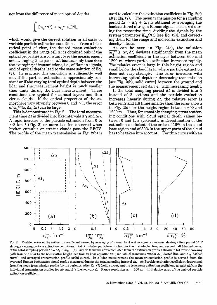
which would give the correct solution in all cases ofvariable particle extinction conditions. From a theo-retical point of view, the desired mean extinctioncoefficient in the range cell Az is obtained only if theoptical properties are constant over the measurementand averaging time period At, because only then doesthe averaging of transmissions, i.e., of Raman signals,and of optical depths lead to the same solution of Eq.(7). In practice, this condition is sufficiently wellmet if the particle extinction is approximately con-stant or if the varying total optical depth between thelidar and the measurement height is much smallerthan unity during the lidar measurement. Theseconditions are typical for aerosol layers and thincirrus clouds. If the optical properties of the at-mosphere vary strongly between 0 and > 1, the errorof ai~xaer(z, Az, At) can be large.

This is demonstrated in Fig. 2. The total measure-ment time At is divided into like intervals At, and At2.A rapid increase of the particle extinction from 0 to-2 km-' (Fig. 2) or more is often observed when

broken cumulus or stratus clouds pass the RFOV.The profile of the mean transmission in Fig. 2(b) is

used to calculate the extinction coefficient in Fig. 2(c)after Eq. (7). The mean transmission for a samplingperiod At = At, + At2 is obtained by averaging thebackscattered nitrogen Raman signals measured dur-ing the respective time, dividing the signals by thesystem parameter KRO(z) [see Eq. (2)], and correct-ing them for the range and molecular extinction anddensity effects.

As can be seen in Fig. 2(c), the solutionaox0aer(z, Az, At) deviates significantly from the meanextinction coefficient in the layer between 600 and1200 m, where particle extinction increases rapidly.The relative error is large in this height region andsmall below the cloud layer, where particle extinctiondoes not vary strongly. The error increases withincreasing optical depth or decreasing transmission[see Fig. 2(b), solid curve] between the ground andthe measurement cell Az, i.e., with increasing height.

If the total sampling period At is divided into 5instead of 2 sections and the particle extinctionincreases linearly during At, the relative error isbetween 2 and 1.6 times smaller than the error shownin Fig. 2(d) for the height region between 600 and1200 m. Thus, for smoothly changing cirrus scatter-ing conditions with cloud optical depth values be-tween 0 and 1, a systematic underestimation of theextinction coefficient of the order of 10% in the cloudbase region and of 30% in the upper parts of the cloudhas to be taken into account. For thin cirrus with an

0 0.5 1 1.5 2 0 0.5 1 0 0.5 1 1.5 2 0 20 40 60 80

Oaer km 1 maer maer 3er k er 0aAo m TAo AR O , km- 6aA 0 %

Fig. 2. Modeled error of the extinction coefficient caused by averaging of Raman backscatter signals measured during a time period At ofstrongly varying particle extinction conditions. (a) Simulated particle extinction for the first (dotted line) and second half (dashed curve)of the total sampling period At = Atl + At2. (b) Particle transmissions calculated from the extinction profiles shown in (a) for the two-waypath from the lidar to the backscatter height [see Raman lidar equation (2)]; individual transmissions for At1 (dotted line) and At2 (dashedcurve), and averaged transmission profile (solid curve). In a lidar measurement the mean transmission profile is derived from theaveraged Raman backscatter signal profile measured during the total sampling interval At. (c) Particle extinction coefficient determinedfrom the mean transmission profile for the period At after Eq. (7) (solid curve), and the true mean extinction coefficient calculated from theindividual transmission profiles for At, and At2 (dashed curve). Range resolution Az = 100 m. (d) Relative error of the derived particleextinction coefficient.


1400

1200

1000

E

0800

600

: i

-ei At2: I- - - - - - - - - -l

:~~~~~~~~~~~~~~~~~~~~~~~~~~:~~~~~~~~~~~~~~~~~~~~~~~~~~:~~~~~~~~~~~~~~~~~~~~~~~~~~

,:At, I:~~~~~~~~~~~~~~~~~~~~~~~~~~

I~~~~~~~~~~~~~~~~~~~~~~~

_ I

: I-:

I

(a).: I. ., I ,

400

200

0

optical depth of 0.2 or less the relative error is below10%.

The question of whether the smoothing of signalsthat can lead to considerable errors in optically thickclouds introduces any additional error was also inves-tigated for the present case. It turned out that in allpractical events of the ICE'89 campaign no additionalerror from sliding data averaging occurred.

Errors of the kind shown in Fig. 2 can be reduced oravoided by dividing the total measurement timeperiod into intervals with constant particle extinctionconditions. The mean extinction coefficient is thenobtained by calculating the extinction profile for eachtime interval and by averaging the resulting extinc-tion profiles. For an appropriate division of the totaltime into intervals signal profiles must be stored withhigh resolution. Time sections of nearly constantparticle extinction can then be determined from thetime series of the elastic-backscatter profiles. But,in general, and this is what we wanted to demonstratewith Fig. 2, one must be careful in the interpretationof measurement results if particle optical propertiesvary strongly, e.g., in inhomogeneous and variablefields of thick cirrus and water clouds.

Averaging the logarithms of the signals, althoughtheoretically leading to the correct solution, is, inpractice, not preferable because of the low signal-to-noise ratio of the raw lidar data profiles and the newsystematic errors introduced by averaging the loga-rithms of noisy data.28

A sufficiently small optical depth throughout theentire measurement region is always given in cloud-free regions, as is the case in Fig. 1(a) below 8 km inheight, in Fig. 1(b), and in optically thin cirrus clouds.In Fig. 1(a), an optically thick cirrus is shown. Theerror, however, is believed to be small because thecloud optical depth, which is determined from the

high-resolution Raman signal profiles for successivetwo-minute intervals, varies smoothly between 0.5and 1. For such a case, the simulation performed asdescribed above (Fig. 2) shows that the extinctioncoefficient in the cloud is underestimated by 10%.

So great care must be taken in the averaging of thelidar signals if the particle scattering properties varystrongly. The error of the particle-extinction coeffi-cient that is due to this effect can be larger than 20%in typical cirrus clouds. The most important atmo-spheric input parameter is the temperature gradient.A significant error can occur if a temperature inver-sion is present and standard atmospheric conditionsare assumed. In practice, because of the combinedeffect of the uncertainties in the estimated ozonedensity, in temperature and pressure profiles, and inthe temperature gradient, an error x0t0aer(z) 0.02km-' must be expected unless temperature and pres-sure data from a radiosonde ascent of a nearbyweather service station are available. This errorcorresponds to 10% in the case of aerosol measure-ments in the boundary layer or in cirrus clouds. Thestatistical error is of the same order of magnitude.It is thus possible to measure cirrus particle extinc-tion properties with a relative error of 20% and withtime and range resolutions of 5 to 20 min and 300 to600 m, provided the scattering properties do not varysignificantly. Multiple scattering contributes lessthan 10% at cloud base and of the order of 5% for theremaining cloud region.

B. Particle Backscatter Coefficient

In Fig. 3 a height profile of the particle-backscattercoefficient that is determined from the ratio of theelastic to the inelastic nitrogen Raman signal byusing Eq. (4) is shown. In addition, the extinctioncoefficient, which is the same as in Fig. (a), and the

0.0 0.2 0.4 0.6 0.8

EXTINCTION COEF., km-'

0.00 0.02 0.04 0.06 0.08

BACKSC. COEF., km-' sr- 10 8 16 24

LIDAR RATIO, srFig. 3. Cirrus particle extinction and backscatter coefficients and the corresponding extinction-to-backscatter ratio for Xo = 308 nm,determined on 24 October 1989 between 1809 and 1821 lt. An ozone density profile according to the standard ozone model for midlatitudeconditions is assumed in the case of the solid curve. The dotted and dashed curves are determined by assuming zero ozone density and anozone concentration that is a factor of 2 higher than the standard model content, respectively.


10.0

9.6

9.2

8.8

8.4

8.0 I . I . I

32

. . . . . . .

resulting extinction-to-backscatter ratio profile aregiven.

In the determination of the backscatter coefficientthe signals of each channel are averaged first. Aftercorrection of atmospheric effects such as the nitrogendensity decrease and the difference of the atmo-spheric transmission for the laser and nitrogen Ra-man wavelengths between the reference height z0 andthe measurement height z [see Eq. (4)], the ratio ofthe averaged and corrected signals is formed andsmoothed. The smoothed signal ratio profile is thenused to calculate the backscatter coefficient accordingto Eq. (4). In Fig. 3, the same sliding average lengthof 300 m is selected as in Fig. 1(a) in the cirrus layer.Again a calculation step width of 60 m is chosen.The reference height is located at z0 = 6 km, whereparticle extinction is low [see Fig. 1(a)]. For thebackscatter boundary value, px 0aer(zO) = 0 is chosen.A proportionality of particle scattering to X-' and XO isassumed below and within the cloud, respectively.Radiosonde data of temperature and pressure areused for the estimation of air density and molecularscattering properties.

A relative systematic error of 5% to 10% that is dueto realistic uncertainties of the estimated ozone den-sity, temperature, and pressure profiles must betaken into account, if no radiosonde data are availableand an ozone density profile according to the stan-dard ozone model is assumed but the true ozonecontent is 0 or a factor of 2 higher than the standardmodel content. The influence of the ozone transmis-sion estimate is shown in Fig. 3. The effect de-creases with decreasing distance z - z0 [see Eq. (4)].It is therefore advisable to set the reference height asclose as possible to the cloud base.

In the case of Fig. 3 the error of pxoaer(z) that iscaused by an uncertainty in the determination of theparticle transmission ratio in Eq. (4) can be neglected.Aerosol transmission between the reference heightz = 6 km and the cloud base is approximately 1 atboth wavelengths because of low particle extinction[see Fig. 1(a)]. The transmission ratio is 1 withinthe cirrus because of negligible wavelength depen-dence of the extinction by ice crystals (see Section 3).The assumption of a weak wavelength dependence ofthe ice-crystal scattering was confirmed by a measure-ment of one lidar group during ICE'89.17

A proportionality of particle extinction in the cirrusto X-' instead of X0 would, in the case of Fig. 3, causean error of the backscatter coefficient of less than 1%.But the wavelength dependence can play a muchmore important role in mixed clouds with high opticalthickness that consist of small water droplets andlarge ice crystals, so that the wavelength dependencevaries between X0 for ice crystals and X-l for waterdroplets. Studies of boundary-layer backscatteringare another example of a case for which the influenceof the wavelength dependence may not be negligible.k and thus Xk is different for different aerosol types.

The error of pX 0aer(z) that is due to the uncer-tainty of the particle reference value pxaer(zo) is

assumed to be small in Fig. 3 because the extinctionprofile shown in Fig. 1(a) suggests a scattering ratioIX3aer/ XOmol 0 at the reference height z = 6 km.As was mentioned, Ioaer(zo)/IX mol(zo) • 0.01 for Xo =308 nm under typical air conditions for the uppertroposphere.25 However, a relative error of 10%occurs if the true reference backscatter ratio

X aer(ZO)/pX mol(zo) = 0.1 instead of 0.Multiple scattering will not affect the determina-

tion of the backscatter coefficient in high-altitudeclouds, after Eq. (4). Strong forward scattering byice crystals or droplets leads to an increase of cloudtransmission. This effect is ratioed out by applyingEq. (4).

As in the case of the extinction-coefficient determi-nation, an additional error of considerable magnitudecan be introduced into the calculation of the back-scatter coefficient if particle scattering propertiesvary strongly during the signal sampling and aver-aging time period At. Here the error of the mea-surement results from the fact that the signals P, 0 (t)and PAR(t), where t denotes the time, are averaged in-stead of the signal ratio Pxo(t) /PR(t). When elastic-backscatter signals are averaged, products of a vari-able backscatter coefficient with a variable transmis-sion are averaged [see Eq. (1)]. The (true) meanbackscatter coefficient is obtained only if the meanelastic-backscatter signal is equal to the product ofthe mean values of the backscatter coefficient and thetransmission term T2 , i.e., if the sum of the prod-ucts of P'(t)T 2 (t), where '(t) and T'(t) are expressedby (t) = + p'(t) and T(t) = TT'(t),is equalto0.

Our theoretical analysis and simulation studiesshow that the averaging effects on the backscattercoefficient and on the extinction coefficient, as pre-sented in Fig. 2, deviate by no more than a fewpercent if a constant relation S 0aer between extinc-tion and backscattering is assumed. Thus, startingfrom Fig. 2(a), calculating the elastic-backscatter andRaman signals after Eqs. (1) and (2) with a constantlidar ratio, separately averaging the signals for thedifferent channels, and, finally, determining the back-scatter coefficient after Eq. (4) will produce approxi-mately the same profiles for aer(z) and SB0 aer(z) asthose of axaer(z) and 8cxaer(z) in Figs. 2(c) and 2(d).According to Fig. 2, the sum of the products I' (t)T '(t)is negligible for only the region below the simulatedcloud layer.

Large errors can be avoided by calculating thebackscatter coefficients separately for the periods At,and At2 and averaging the obtained values. Theoret-ically the averaging of the signal ratios could lead tothe correct solution, provided that the signals can bestored with sufficient time resolution and that thesignal-to-noise ratio of the raw data is high. Inpractice, the signal-to-noise ratio is low, especially forthe Raman signals, and the same considerations asthose developed in Subsection 4.A for the extinctioncoefficient also apply to the determination of backscat-ter coefficients.

In conclusion, again nearly constant optical proper-


ties or, under variable atmospheric conditions, opticaldepth values below 0.5 are needed during the signalaveraging period At in order to avoid relative errorslarger than 20%. The combined effect of uncertain-ties in ozone density, temperature, and pressure onbackscatter coefficient profiles may result in a relativeerror of 10%. The reference height should be setjust below the cloud to minimize the error from theuncertainty in the estimates of the molecular andparticle transmissions between z0 and the measure-ment height z. A relative statistical error of lessthan 10% in combination with high depth resolutioncan be achieved only in regions of strong backscatter-ing, i.e., in clouds and in the boundary layer.

C. Lidar Ratio

The atmospheric input parameter that most affectsthe solution of Eq. (5) is the ozone density. Anunderestimation of the ozone content leads to anoverestimation of the particle extinction coefficient[which is the numerator in Eq. (5)] and an underesti-mation of the backscatter coefficient [which is thedenominator in Eq. (5)] and vice versa. In the caseof cirrus observations, the error of the lidar ratio thatis due to the ozone uncertainty is of the order of 5% to10% (see Fig. 3). An additional 5% can occur ifstandard atmosphere profiles for the temperatureand pressure are assumed, i.e., if no actual radiosondedata are available.

The analysis in Subsections 4.A and 4.B shows thatthe error from uncertainties in the estimate of theparticle wavelength exponent k used in Eqs. (3) and(4) and of the reference value pxoaer(zo) used in Eq. (4)can be neglected in the case shown in Fig. 3. Themultiple-scattering effect is the same as for theextinction coefficient, i.e., between 5% and 10%.

Rapid temporal changes of the aerosol extinctionproperties do not affect the determination of SX0er ifthe lidar ratio is constant during the measurementinterval because then 8P/ = 8/ax (see Subsection4.B). If both the lidar ratio and the particle extinc-tion coefficient vary, the measured lidar ratio isdetermined mainly by the periods of strong particlescattering, as the simulations and the evaluation ofthe lidar data show. Assuming, e.g., in Fig. 2 a lidarratio of 10 instead of 20 sr within the cloud layerduring At2, we obtain a lidar ratio for the total time Atof 10 sr at the bottom and 12.5 sr at the top of thecloud instead of the mean value of 15 sr. It can thusbe concluded that varying optical properties do notsignificantly affect the determination of cloud lidarratios. For the case shown in Fig. 3 and also for themeasurements presented in Subsection 4.D no signif-icant errors are introduced by signal and signal ratiosmoothing.

A critical point in the error analysis is the estima-tion of the influence of specular reflection by fallingice crystals that are horizontally oriented. Whereassmall particles have no preferred orientation, crystalsof typical cirrus particle size sink with their longestaxes parallel to the ground.3 Horizontal alignment

gives the maximum resistance of motion. Largeparticles begin to oscillate. A persistent flutteringoccurs. Crystals oriented precisely horizontally causea large backscatter signal by specular reflection.Few oriented crystals are believed to be able toproduce strongly enhanced backscattering and a lowlidar ratio.33 If this is true, specular reflection, oftenobserved in cirrus with a vertically pointing lidar,34

will dominate all experimentally determined lidarratio values. However, recent measurements per-formed with our lidar tilted by 28 mrad do notconfirm this assumption, as a tilt angle of greaterthan 5 mrad should be sufficient to ensure that nospecular reflection affects the lidar results.34 Againextinction-to-backscatter ratios between 5 and 20 srwere observed in most cases. Only in a few excep-tional cases were large lidar ratios > 30 sr, which areassumed to be caused by specular reflection, deter-mined with the tilted system. If the lidar is tilted,photons backscattered from horizontally orientedcrystals cannot enter the receiver telescope. So webelieve that specular reflections do not play thatimportant a role. At least, in many measurementcases, scattering properties of randomly orientedparticles are measured with the vertically pointingcombined lidar.

In summary, the combined lidar permits the deter-mination of the lidar ratio with a relative statisticalerror of 15% to 30% and a range resolution of 300 to600 m in high-level clouds. Compared with theinfluence of varying optical properties during thesignal averaging time on ax aer and pX0aer, the effect onSX0 aer is small. The most important atmosphericinput parameter is the ozone density profile. Thetotal relative systematic error is of the order of 10% to20%.

D. Particle Extinction Coefficients from Klett's InversionMethod

A large number of papers have been published inwhich the error of the Bernoulli solution for theparticle extinction coefficient is analyzed (see, e.g.,Klett,8 ,35 Fernald,9 and Bissonnette36). The discus-sion of the applicability of the Klett inversion proce-dure to cloud investigations will, therefore, be re-stricted here to aspects that have not been sufficientlyconsidered until now. Extinction profiles obtainedwith the inversion method [Eq. (6)] and the Ramanmethod [Eq. (3) or Eq. (7)] are presented for twocases, one with a nearly height-independent extinc-tion-to-backscatter ratio (in this section) and onewith a range-dependent lidar ratio (in Section 5).

In general, great care must be taken in the interpre-tation of the Bernoulli solution for the particleextinction coefficient. As is well known in the lidarcommunity, the inversion method suffers from thefact that two physical quantities, the particle backscat-ter and the particle extinction coefficients, must bedetermined from only one measured lidar signal.To solve Eq. (6), we must make assumptions aboutthe relation between the two, and we need an esti-


mate of the boundary value of the aerosol extinctioncoefficient. These data, Saer(z) and crxaer(zo), areusually hard to assess and can cause large uncertain-ties in the aerosol extinction coefficient.

Most devices designed as backscatter lidars havebeen operated in the visible and the infrared parts ofthe spectrum. UV devices offer a big advantage inthat the correct estimate of the boundary value, atleast at the far end of the lidar range, is much easierto obtain because of strong Rayleigh scattering. Onthe other hand, a drawback of a system measuring at308 nm is the onset of UV ozone absorption at thiswavelength. A relative error of more than 20% mustbe faced under unfavorable conditions for the cirrusparticle extinction coefficients owing to the uncer-tainty in the estimate of the ozone optical depthbetween the reference height z0 and z (see Section 3).The effect is minimized if z0 is close to the cloudbase. The ozone influence is much more importanthere than in the determination of xx0aer from theRaman signals because the round-trip absorption at308 nm is so much larger than the additional absorp-tion of the 332-nm Raman backscatter radiation.

The remaining problem is the estimation of thelidar ratio. Depending on aerosol type, S 0aer canvary over orders of magnitude. In practice, no infor-mation on the required height profile of the lidar ratiois usually available.

An average value of the lidar ratio can be obtainedin the case of sufficiently constant microphysicalcloud conditions in both space and time. A trialvalue is taken for the lidar ratio, and Eq. (6) is solvedby forward integration. If the solution is unstable,another, lower trial value is used until a stablesolution results. The same trial value is then usedfor the backward integration of Eq. (6). Normallythe resultant profiles of the extinction coefficient willdiffer. The trial value can then be varied until theresults of the forward and backward integrationcoincide to the desired degree of accuracy. Usually

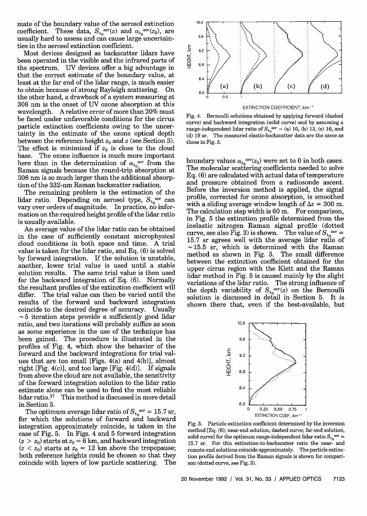
5 iteration steps provide a sufficiently good lidarratio, and two iterations will probably suffice as soonas some experience in the use of the technique hasbeen gained. The procedure is illustrated in theprofiles of Fig. 4, which show the behavior of theforward and the backward integrations for trial val-ues that are too small [Figs. 4(a) and 4(b)], almostright [Fig. 4(c)], and too large [Fig. 4(d)]. If signalsfrom above the cloud are not available, the sensitivityof the forward integration solution to the lidar ratioestimate alone can be used to find the most reliablelidar ratio.37 This method is discussed in more detailin Section 5.

The optimum average lidar ratio of SX0aer = 15.7 sr,for which the solutions of forward and backwardintegration approximately coincide, is taken in thecase of Fig. 5. In Figs. 4 and 5 forward integration(z > z) starts at z0 = 6 km, and backward integration(z < z0 ) starts at z0 = 12 km above the tropopause;both reference heights could be chosen so that theycoincide with layers of low particle scattering. The

10.0

9.6

E

IY

9.2

8.8

8.0 0 0.5 1

EXTINCTION COEFFICIENT, km-'

Fig. 4. Bernoulli solutions obtained by applying forward (dashedcurve) and backward integration (solid curve) and by assuming arange-independent lidar ratio of S,\Oaer = (a) 10, (b) 13, (c) 16, and(d) 19 sr. The measured elastic-backscatter data are the same asthose in Fig. 3.

boundary values cAX aer(zO) were set to 0 in both cases.The molecular scattering coefficients needed to solveEq. (6) are calculated with actual data of temperatureand pressure obtained from a radiosonde ascent.Before the inversion method is applied, the signalprofile, corrected for ozone absorption, is smoothedwith a sliding average window length of Az = 300 m.The calculation step width is 60 m. For comparison,in Fig. 5 the extinction profile determined from theinelastic nitrogen Raman signal profile (dottedcurve, see also Fig. 3) is shown. The value of SA aer =

15.7 sr agrees well with the average lidar ratio of15.5 sr, which is determined with the Raman

method as shown in Fig. 3. The small differencebetween the extinction coefficient obtained for theupper cirrus region with the Klett and the Ramanlidar method in Fig. 5 is caused mainly by the slightvariations of the lidar ratio. The strong influence ofthe depth variability of Saer(z) on the Bernoullisolution is discussed in detail in Section 5. It isshown there that, even if the best-available, but

10.0

9.6

E

I9.2

8.8

8.4

8.0

0 0.25 0.50 0.75 1EXTINCTION COEF., km-'

Fig. 5. Particle extinction coefficient determined by the inversionmethod [Eq. (6); near-end solution, dashed curve; far-end solution,solid curve] for the optimum range-independent lidar ratio Sx0aer =15.7 sr. For this extinction-to-backscatter ratio the near- andremote-end solutions coincide approximately. The particle extinc-tion profile derived from the Raman signals is shown for compari-son (dotted curve, see Fig. 3).


height-independent, lidar ratio is used, large uncer-tainties in the particle extinction profile remain.

An additional aspect must be discussed here thathas not, in the authors' opinion, been sufficientlyconsidered in the Klett error analysis until now. Asin Subsections 4.A and 4.B, a significant error can beintroduced into the calculation if the scattering prop-erties vary strongly during the signal sampling andaveraging time period At. This is demonstrated inFig. 6.

The error results from the fact that the elastic-backscatter signal depends on a variable backscattercoefficient 13 and a variable transmission term T2 [seelidar equation (1)]. Let 13 and T be expressed here as

W(t) = + '() with the mean value 13 and thedeviation 13'(t) and T(t) = TT*(t), where T is thetransmission corresponding to the mean optical depthfor the time period At, from which the desiredextinction coefficient can be determined, and T* (t) isused to describe the deviation of T(t) from T. Thetrue mean particle extinction coefficient [Fig. 6(c),dotted curve] is then obtained if the average of13'(t)T*2(t) is equal to 0. This is approximately the

case in Fig. 6 below and above the layer of stronglyvarying particle extinction conditions. The value of13' (t) T*2 (t) and, thus, the error of the Klett solutions

increase with height.

E

0WI

1400

1200

1000

800

600

400

200

00 0.5 1 1.5 2

a aer km-1

As stated above large errors as shown in Fig. 6 maynot play an important role in studies of optically thincirrus clouds as long as rapid and large variations ofthe optical depth are absent, but must be taken intoaccount in measurements in inhomogeneous waterclouds in which the particle extinction coefficient canvary between values near 0 and 30 km-' within a fewseconds.

In summary, the error of the Bernoulli solution interms of the particle extinction coefficient can belarge because of the large uncertainty of the estimatefor the lidar ratio Saer in Eq. (6). If both theforward and the backward integration variant of theKlett method can be applied, which usually holds foroptically thin clouds, and the near- and far-endboundary values are well estimated, an appropriateaverage lidar ratio can be determined and the error inthe determination of Uaaer(z) can be minimized. At308 nm, a good calibration is possible because ofstrong Rayleigh scattering. On the other hand, agood estimate of ozone absorption is required. As inthe case of the Raman lidar, care must be taken in thestudy of inhomogeneous clouds.

An advantage of the Klett method over the Ramanlidar method is the fact that particle scattering isdetermined from a strong elastic-backscatter signalthat is several orders of magnitude larger than the

0 0.05 0.1 0 0.5 1 1.5 2 0 25 50 75 1 00

3aer TT 2 km sr1 aer km t !a-er3 T km-'sr-` aA",k -'6'! Fig. 6. Modeled particle extinction coefficients determined from elastic-backscatter signals measured during a time period of stronglyvaryingparticle extinction conditions. (a) Assumed particle extinctions during the first (dotted curve) and second (dashed curve) halves ofthe total sampling period At = At, + At2. For simplicity, molecular scattering and extinction are neglected. (b) Range-correctedelastic-backscatter signal assuming 100W(z) = 1 in the lidar equation (1). The profiles for the time sections At1 (dotted curve) and At2(dashed curve) are calculated with the extinction coefficients shown in (a) and an aerosol lidar ratio of 20 sr. The solid curve is obtained byaveraging the profiles for At1 and At2. (c) Particle backscatter coefficient determined from the mean corrected signal profile [(b), solidcurve] by using the Klett method in the forward (dashed curve) and backward (solid curve) integration mode. The reference heights arez = 100 m (forward integration) and 1400 m (backward integration). The correct boundary value of 0.2 km-' and the correct lidar ratioare taken for the retrieval. The calculation step width is Az = 100 m. The corresponding true mean extinction profile according to (a) isshown for comparison (dotted curve). (d) Relative error of the particle extinction coefficients derived by applying forward (dashed curve)and backward (solid curve) integration.


I~~~~~~~~~~~~~~~~~~~~~~~

: ~~~~~~~~~~~~~~~~~~~I.~~~~~~~~~~~~~~~~~~~~~~~~~~~~~~~~~~~

. ~~~~~~~~~~~~~~~~~~~~~~~~I'.At, I

. ~~~~~~~~~~~~~~~~~~~~~~~~I

I~~~~~~~~~~~~~~~~~~~~~~~I~~~~~~~~~~~~~~~~~~~~~~~:~ ~~ -- I

_ I- - -: I

I: I

: i (a): I

-~~~~~~~~~~~ I

-1L

\\ :

- II\

At

I I. . . .

Raman signal. The Klett method can thus be ap-plied during the daytime. The statistical error fromsignal noise is small, and high temporal and spatialresolution can be achieved. The influence of vari-able scattering conditions during signal averagingperiods is reduced by the possibility of short averag-ing intervals.

5. Experimental Results and Discussion

In this section examples of independent measure-ments of the extinction and backscatter profiles inhigh-altitude clouds and, thus, of the lidar ratioprofile are presented and discussed. Based on an-other comparison of the Bernoulli with the Ramanlidar solution and on the results of a cirrostratusmeasurement, the applicability of the Klett inversionmethod to cloud studies is illustrated.

The results shown in the figures below have beenobtained with the combined Raman elastic-backscat-ter lidar. The statistical error, which is due tophoton noise, and, in the case of lidar ratio observa-tions, the systematic error resulting from the uncer-tainity in the assumed ozone density (see Section 4)are indicated by error bars and dashed curves, respec-tively. Other systematic errors can be neglectedhere, especially since the temperature and pressureprofiles were measured with radiosondes launched atthe lidar station. Layers of low particle scatteringwere present below the cloud in all cases shown. Thisjustifies the use of the reference value PxBaer(zo) = 0

and the neglect of the error introduced by 8,\Oaer(zo).The calculation step width is 60 m.

In Fig. 7, a cirrostratus measurement is shown.The atmospheric conditions on that day were uniqueduring the field campaign of ICE'89 in that opticaland geometric properties of the cloud deck remainedapproximately unchanged with time and height formore than 3 h. Only in this particular case could the

average of a 2-h measurement be taken withoutmaking a large error. Most of the 2-min averagevalues of the cloud optical depth, derived from therespective high-resolution Raman signal profiles, arebetween 0.2 and 0.5. According to the discussion inSubsections 4.A and 4.B, the extinction and backscat-ter coefficients shown in Fig. 7 are estimated to be lessthan 10% and 20% too small for the lower cloudregion and the main cloud layer between 10.5 and11.6 km in height, respectively, despite the longaveraging time.

The cloud temperatures range from - 380C at 9 kmto - 580C at the top of the cirrus, which coincides withthe tropopause. The similarity of the extinction andbackscatter profiles suggests a close relation betweenthe mean transmission and reflection properties.The mean optical depth, derived from the extinctioncoefficient, is 0.38. Taking into account the effectsof smoothly changing extinction conditions and multi-ple scattering (5% to 10%, see Section 4), we obtain asingle-scattering optical depth of the order of 0.5.

The vertical distribution of the lidar ratio suggestsdifferent microphysical characteristics in the lowerand upper parts of the cloud. However, the interpre-tation of the experimentally determined extinction-to-backscatter ratios is difficult because of the largeerrors, as indicated in Fig. 7, of the unknown influ-ence of specular reflection and of the range depen-dence of multiple scattering, which is also unknown.

Nevertheless, there are two good reasons to believethat the measured data are typical for cirrus scatter-ing conditions, i.e., scattering by mainly randomlyoriented crystals. First, our recent cirrus measure-ments with a tilted lidar show, in most cases, nosignificant differences in the results obtained underzenith angles of < 1 mrad and 28 mrad. Second, andmore important, the determined lidar ratios agreewell with theoretical values inferred from numerical

12.0

11.4

E

ICD7nj

10.8

10.2

9.6

9.00 0.15 0.3 0.45 0.6 0 0.015 0.03 0.045 0.06 4 8 12 16 20

EXTINCTION COEF., km-1 BACKSC. COEF., km- 1 sr-1 LIDAR RATIO, srFig. 7. Particle extinction and backscatter coefficients and the corresponding lidar ratio determined in a cirrostratus cloud on 24 October1989 between 1854 and 2042 t. 725,600 laser shots are averaged. Signal smoothing lengths are Az = 600 m for z < 10.5 km and 300 mfor z 2 10.5 km. Rayleigh extinction and backscatter coefficients (dotted curves) are shown for comparison.


I -

II4

= . . . . .

calculations3 0 in which, for observed ice-crystal sizedistributions of a cirrostratus,38 cold (-550 C) andwarm (-30'C) cirrus clouds,39 and a cirrus uncinuscloud38 with a considerable amount of large ice crys-tals with lengths > 500 rim, the scattering phasefunction was determined for = 550 nm with theassumption of randomly oriented hexagonal ice crys-tals. According to these calculations the lidar ratiois 10 sr for typical cirrus clouds, including cirrostra-tus, and 17 sr for cirrus uncinus, i.e., for an ice cloudwith more larger particles. The scattering phasefunction for randomly oriented and small hexagonalplates (diameter, 20 Aim) and columns (length, 120pum) and a wavelength of X = 632 nm yields a lidarratio between 5 and 10 sr.4 0

It must be stated here that this is, to our knowl-edge, the first time that experimentally derived lidarratios agree in a satisfactory way with results oftheoretical studies. Mean cloud lidar ratios between30 and 80 sr, frequently > 40 sr, were obtained withthe so-called lidar and infrared radiometric (LIRAD)method. 4 ,42 During FIRE'86, mean cloud lidar ra-tios between 15 and 50 sr, frequently between 25 and35 sr, were determined by the use of the HSRLtechnique.' 3 None of these attempts to reproduceexperimentally the small lidar ratio values of themodels was successful.

It is unclear at the present time how much of thesediscrepancies may be caused by the fact that, innumerical calculations, crystals are modeled simplyby hexagonal plates and columns, or spheres. Assem-blies of real ice crystals, however, contain partlycomplex shapes, depending on water vapor pressure,which increases with temperature, and on the strengthof vertical motions at different scales in the uppertroposphere. Results of numerical calculations ofthe extinction-to-backscatter ratio for ice clouds com-posed of irregularly shaped ice particles such as bulletrosettes would be useful for clarifying the differencesbetween model and experimental results. Ideallyshaped crystals, as assumed in the models, are possi-bly more frequently present in cirrus clouds at higherlatitudes (>50'N or ) where convective processesmay be relatively weak compared with those intropical and lower midlatitude regions. ICE'89 tookplace in the German Bight of the North Sea at>530N. FIRE'86 and other lidar ratio measure-ments were performed near 40'N and S or at lowerlatitudes.

The numerical studies imply a decrease of the lidarratio with a decreasing size of scattering ice crystals.The lidar ratio profile in Fig. 7 may thus indicate thepresence of smaller particles in the layer of strongbackscattering and larger particles in the layer below.Evaporation of ice crystals in the fall-streak regionbelow 10.5 km must also be taken into account.Laboratory studies43 show that the corners of parti-cles become rounded during evaporation, and parti-cles probably change their scattering properties.Comparisons with studies of scattering properties ofdroplets44 ,45 indicate that spheres with diameters

within the atmospheric range between 0.1 and 100pLm exhibit a larger lidar ratio, between 15 sr and 60sr, than hexagonal crystals of atmospheric ice clouds.Breakup was found to take place when the relativehumidity drops below 70% related to ice.43 In thisway, many small particles that cause a lowering of thelidar ratio may be produced.

With respect to cirrus studies with an elastic-backscatter lidar, the above discussion makes clearthat a range-variable lidar ratio must generally betaken into account if the Klett method is applied,whether or not specular reflection is present. Theerror introduced in the Bernoulli solution by a range-independent extinction-to-backscatter ratio is dis-cussed below.

How specular reflection influences the extinction-to-backscatter ratio can be seen in Fig. 8. The measure-ment was performed in the last of several cirrusbands crossing the lidar station in a weak southwest-erly airflow. Temperatures between -25C and-40°C were measured by radiosonde between 7 and 9km. The optical depth of the cirrus is estimated tobe again -0.5 ± 0.1.

As can be seen, a nearly range-independent extinc-tion coefficient is found, whereas the backscattercoefficient increases with height, with a strong maxi-mum in the upper cirrus region. The correspondingprofile of the lidar ratio shows typical cirrus values forheights below 8 km, a sharp decrease at about 8 km,and extremely small values of 2 to 3 sr in the uppercloud region, which are presumably caused by a layerwith a considerable amount of horizontally orientedice crystals. This result is in agreement with numer-ical calculations.3 3 Such low lidar ratios cannot beexplained by multiple scattering, which affects theresults by 10% only. The large lidar ratio valuesat the bottom of the cloud may result from thepresence of large crystals, ice spheres, or supercooledwater droplets. The temperature at 7 km in heightwas only -25°C. Water droplets, possibly present incirrus clouds at temperatures > -400 C,46 lead to anincrease of the lidar ratio. The deviation of theextinction from the backscatter profile in the case ofFig. 8 clearly demonstrates that the reflection proper-ties of cirrus clouds depend quite significantly onwhether the ice crystals are oriented randomly or in ahorizontal plane.47 Particle number density appearsto be nearly constant with height in the present casebecause the extinction coefficient, which is primarilya function of particle density, is almost range indepen-dent.

Figure 9 shows two measurements of an inhomoge-nous cirrus deck that remained after the passage of acold front. A fibrous cloud covering the entire skyand consisting of long ice-crystal streamers and fila-ments could be observed in the moonlight. Strongwinds were present in the upper troposphere. Tem-peratures ranged between -36°C at 7.5 km and-41°C at the top of the cirrus layer at 8.5 km.Because of rapidly varying scattering and extinctionconditions during the measurement, the relative er-


0 0.25 0.5 0.75 1

EXTINCTION COEF., km-'

0 0.025 0.05 0.075 0.1

BACKSC. COEF., km- 1 sr-0 6 12 18 24

LIDAR RATIO, sr

Signal smoothing length is Az = 300 m. Profiles of Rayleigh extinction and backscattering (dotted

ror of pxoaer(z) may be larger than 20%. The errorintroduced by the uncertainty in the ozone densityestimate, not shown in Fig. 9, is of the same order asthat shown in Fig. 8.

The two measurements were taken within 30 min.In the phase of weak backscattering, a lidar ratio of-5 sr was measured. For strong backscattering,- 10 min later, a lidar ratio of greater than 10 sr was

found. According to the profiles of xaer and SX0aer,

the extinction coefficient (a = S1) increases withtime by a factor of 4, while the backscatter coeffi-cient increases by only a factor of 2. The examplesagain illustrate that care must be taken when extinc-tion properties are inferred from elastic-backscatterdata alone, with the assumption of a time-invariantand range-independent lidar ratio. In Fig. 9, thetypical range of cirrus lidar ratios measured during

the ICE'89 campaign is presented. Extinction-to-backscatter ratios between 5 and 15 sr were usuallyobserved.

Finally, in Fig. 10, a measurement in a water cloud(altostratus) is shown for comparison. Since thelidar system was optimized for the observation ofhigh clouds, only a few water cloud cases could befound. In addition, strong extinction often preventsa measurement of the Raman signal profile withinthe cloud.

The measurement was performed in the late eveningof 24 October in a stable and homogenous altostratuscloud with an optical depth of 2 and a meantemperature of -8°C. The optical depth varied be-tween 0.6 and > 2 during the passage of the altostra-tus cloud field. A relative error of the order of 50%must be taken into account for ot, aer (see Subsection4.A). The influence of varying optical properties on

E

ICD7

8.60

8.36

8.12

7.88

7.64

7.400 0.05 0.1 0.15 0.2

BACKSC. COEF., km- 1 sr 10 5 10 15

LIDAR RATIO, sr

5.00

4.92

E

ID

4.84

4.76

4.68

20

Fig. 9. Particle backscatter coefficient and extinction-to-backscat-ter ratio determined in a cirrus cloud on 13 October 1989 at 2119(dashed curves) and 2138 lt (solid curves). 107,099 and 21,528laser shots sampled in 10 min and 2 min are averaged, respectively.The data smoothing length is Az = 360 m. The Rayleigh backscat-ter coefficient is given by a dotted curve.

4.600 3.5 7 10.5 14 5 10 15 20 25

EXTINCTION COEF., km- 1 LIDAR RATIO, sr

Fig. 10. Particle extinction coefficient and extinction-to-backscat-ter ratio determined in an altostratus cloud on 24 October 1989 at2225 lt. 18,140 laser shots sampled in 2 min are averaged.Spatial resolution is 60 m. The comparably small Rayleigh extinc-tion coefficient is given by the dotted curve.


9.0

E

0IU

8.5

8.0

7.5

7.0

6.5

98,358 laser shots are averaged.curves) are also plotted.

Fig. 8. Cirrus scattering properties determined with a combined lidar in a cirrus cloud on 20 September 1989 between 0447 and 0456 lt.

the lidar ratio are estimated to be small (see Subsec-tion 4.C).

The lidar ratio profile agrees sufficiently well withresults obtained in laboratory measurements for real-istic atmospheric droplet spectra. In one study44

lidar ratios between 17 and 19 sr were found forpolydisperse clouds with a broad spectrum of dropletsizes and for a measurement wavelength of X = 632nm. From another study45 at X = 514 nm it can beconcluded that the lidar ratio is between 15 and 23 srfor atmospheric water clouds of low optical depth andcorrespondingly low extinction coefficients, as is thecase in Fig. 10. Also, a decrease of the extinction-to-backscatter ratio with increasing droplet size wasfound.46 Keeping in mind that our measurementswere performed at = 308 nm, that the laboratoryanalysis also suggests a decrease of the lidar ratiowith decreasing wavelength for a given droplet spec-trum, and, finally, that a small multiple-scatteringeffect must be taken into account in lidar measure-ments in high altitude water clouds even for smallRFOV's, which also leads to a decrease in the lidarratio, we find that the measured cloud extinction-to-backscatter ratios agree well with the laboratoryresults.

In the last part of this section, the applicability ofthe Klett inversion method to studies of cirrus opticalproperties is illustrated. It is shown that, althoughthe extinction-coefficient profile can be incorrect be-cause of the unrealistic assumption of a range-independent lidar ratio, the determined backscatter-coefficient profile, the cloud optical depth, and themean cloud extinction-to-backscatter ratio can still beobtained with high temporal resolution and accept-able accuracy.

In Subsection 4.D a first comparison of extinctionprofiles obtained with Eq. (6) (the Bernoulli solution)and Eq. (3) or Eq. (7) (Raman lidar solution) for thecase of a nearly range-independent extinction-to-backscatter ratio was shown (see Fig. 5). The agree-ment was good. In Fig. 11, a second comparison ispresented for the case of a strongly range-dependentlidar ratio S, aer(z). The measured elastic-backscat-ter data are the same as those of Fig. 8. Theoptimum range-independent lidar ratio of 7.3 sr forwhich the solutions of backward (solid curve) andforward (dashed curve) integration nearly coincide isselected. The near-end (z = 6.4 km) and remote-end (z = 9.4 km) boundaries of the integration areset into regions with dominant Rayleigh scattering[axmoml(zo) >> ax0 (zo)] so that the errors of theboundary values are assumed to be small. Beforethe inversion technique is applied, ozone absorptioneffects are corrected, and the corrected signal profileis smoothed with a gliding average window length ofAz = 300 m. The ozone optical depth is 0.03 for X0 =308 nm between the two reference heights accordingto the standard ozone model. Thus, considering anozone uncertainty of ± 100% as before, we get arelative error of the extinction coefficient and of theparticle optical depth of the order of 10%.

9.0

8.5

E

C8.0

7.5

7.0 g,,.>

6.5 . ' . ' . L f . f 0.0 0.2 0.4 0.6 0.8 0 0.125 0.25 0.375 0.5

EXTINCTION COEF., km-' OPTICAL DEPTH

Fig. 11. Particle extinction coefficient (right) and resultingopticaldepth (left) determined from the elastic-backscatter signal at 308nm by using the Klett method in the forward (dashed curve) andbackward integration mode (solid curve). The measured data arethe same as those in Fig. 8. A range-independent lidar ratio ofS,0 aer = 7.3 sr is assumed. For this lidar ratio the near-end andfar-end solution coincide approximately. For comparison (dottedcurves) the particle extinction profile and the corresponding opticaldepth determined after the Raman lidar method are also shown.

No similarity of the Bernoulli and the Raman lidarsolutions can be seen. This is due to the strongvariation of the lidar ratio with height (see Fig. 8).Only with S,0aer(Z) shown in Fig. 8 would the correctsolution follow. By using a range-independent lidarratio (and an alternative to this assumption is notavailable) we find that the obtained profile of theextinction coefficient is similar only to the backscattercoefficient profile in Fig. 8. The reason is that incases of weak attenuation, the elastic-backscattersignal, corrected for range and molecular absorptionand scattering effects, is mainly a function of theparticle backscatter coefficient [see Eq. (1)].

Figure 11 underlines that reliable height profiles ofthe extinction coefficient cannot be determined withthe Klett method. Only the profile of the backscat-ter coefficient is acceptable. On the other hand, theapplication of both forward and backward integrationyields the mean cloud lidar ratio of SA aer = 7.3 sr (seeFig. 8) along with the mean optical depth of the cloudof 0.42. We should mention that the technique isequivalent to the method in which the cirrus opticaldepth is determined from the Rayleigh backscattersignals from below and above the cloud and used toconstrain a Bernoulli solution to the extinction pro-file, the range-independent lidar ratio, and the back-scatter coefficient profile.'3

Figure 12 illustrates the variability of the meancloud lidar ratio with time and, again (see Fig. 4), thesensitivity of the solution of forward integration tothe S,0aer estimate. A short section of a cirrostratusmeasured on 18 October 1989 is selected. The refer-ence heights of forward and backward integration areset to z = 6 and 12 km (above the tropopause),respectively; cjaaer(Zo) = 0 is taken. The calculation inFig. 12 is performed with the lidar ratio S 0aer = 13 sr.This value is appropriate for the determination ofcases (c) and (d) in Fig. 12. It is too large for the


12.5

11.7

E

LLT

10.9

10.1

9.3 jw Vll 4(a) | (b) (c) (d) i (e) ! (f)

8.5 l I l I l l

0 0.4 0.8

EXTINCTION COEFFICIENT, km-1

Fig. 12. Bernoulli solutions applying forward (dashed curve) and backward (solid curve) integration. The lidar measurement was takenin a cirrostratus deck on 18 October 1989 between 1129 and 1144 lt. Approximately 6,300 laser shots are averaged for each profile sampledin 150 s. Spatial resolution is 60 m. A lidar ratio Sx0aer = 13 sr is selected. This lidar ratio can be seen to be appropriate in cases (c) and(d) only.

other cases. Forward integration begins to becomeunstable in case (e), and is completely unstable in case(f). Optimum range-independent lidar ratios are 10,11.5, 7, and 5 sr for cases (a), (b), (e), and (f),respectively. The mean cloud lidar ratio varies be-tween 5 and 15 sr within a few minutes.

Our experience shows that for cirrus clouds of lowoptical depth, below 0.5, the optimum extinction-to-backscatter ratio is roughly one half of the lidar ratiofor which the forward integration solution becomesunstable. This result, which only holds for opticallythin cirrus, was also found in a previous study37 inwhich the forward integration method alone was usedto determine the optimum cloud lidar ratio. Such alow cirrus optical depth was given over the whole dayon 18 October 1989. Figure 13 summarizes theresults of the measurement taken on that day. Thetime series of the cloud lidar ratio is shown in Fig.13(d). Most of the Bernoulli solutions of forwardintegration became unstable for lidar ratios between15 and 20 sr.

Figure 13 illustrates the usefulness of the Klettmethod for cirrus studies. For 115 profiles of theelastic-backscatter signal the optimum height-aver-aged lidar ratio is determined and used for thecalculation of the maximum backscatter coefficientand the cloud optical depth. The ozone optical depthfor the region between the two boundary heights of 6and 12 km is 0.07 according to the standard model.Considering again an ozone uncertainty of ±100%,we find that the relative error of the optical depth andof the cloud lidar ratio is 15%, 30%, and > 50% for

optical depths of 0.4, 0.2, and less than 0.1, respec-tively.

A closed cloud deck with rather smooth structuresis observed for more than 5 h. Low wind speed (<15m/s) and temperatures between -420C (9 km) and-60'C (11.7 km) are measured in the cirrus layer.The cloud begins to form at the tropopause in themorning, one hour before the measurement wasstarted, and disappears near sunset. The time seriesof the cloud top and base heights show a relativelylarge geometrical extension of the cloud that is persis-tent over several hours. While the cloud top isapproximately constant, the base height varies consid-erably as a result of ice-crystal fall streaks crossingthe RFOV.

Large maximum backscatter coefficients are ob-served between 1130 and 1230 It, certainly caused byfalling and, thus, horizontally oriented crystals.Together with the large backscatter peak at 1220 It avery low lidar ratio of 2 sr is determined. As indi-cated in Fig. 13(a) (dashed curve), most of the maxi-mum backscatter values, measured during the firsthalf of the period shown, are found near the cloudbase. Particle trails lead to a rapid increase of thecirrus geometric depth. In periods with low maxi-mum backscatter coefficients, below 0.05 km-'sr-',as is the case between 1440 and 1520 lt, the variabil-ity of the maximum backscatter height is largest.These variations appear to be caused by densityfluctuations of the relatively homogeneously distrib-uted particles. This interpretation is confirmed bythe time series of backscatter height profiles. Sharp


12

A 11

= 10

8

0-40

ugm

x

0.80.60.4

0.20.0

0.80.60.40.20.0

2015

10

50

11 12 13 14 15 16

LOCAL TIME

Fig. 13. Time series of cirrus top and base heights [(a), solidcurve], the height at which the backscatter coefficient takes itsmaximum [dashed curve in (a)], cloud optical depth (b), maximumbackscatter coefficient (c), and cloud lidar ratio (d) determinedfrom the elastic backscatter signals by using the Klett method.The measurement was taken on 18 October between 1043 and1628 lt. The temporal resolution is 150 s. The cloud lidar ratiois obtained by applying forward and backward integration. Themaximum backscatter coefficient and the cloud optical depth arecalculated with the shown cloud lidar ratio. RAT, ratio; BS,backscatter.

backscatter peaks, observed during the first half ofthe experiment, were seldom in the second half until1520 lt, when the cloud began to dissolve.

The cloud optical depth is almost constant over thewhole day. The strongest variability is observed inthe middle and at the end of the cirrus life cycle.Small cloud lidar ratios are found that may indicatethat the cirrus is composed mainly of small icecrystals.

6. Summary

For the first time to our knowledge, independentmeasurements of the backscatter and extinction pro-files in high-level ice clouds have been made with acombined Raman elastic-backscatter lidar. The er-ror analysis shows that realistic uncertainties in theatmospheric input parameters lead to relative system-atic errors of the determined cirrus optical parame-ters of 10% to 20%. An additional error of more than50% can be introduced if the optical properties varystrongly during the signal sampling and averagingperiod. Using the combined lidar technique, we canobtain height profiles of cirrus extinction, backscat-ter, and lidar ratio with a range resolution of 300 to600 m, a time resolution of 5 to 20 min, and astatistical error of less than 20%.

Measurement examples obtained during ICE'89indicate that the extinction and backscatter profilesof cirrus clouds can significantly differ from eachother because of the dependence of the backscattercoefficient on shape, size, and orientation of theanisotropic ice particles, and they also indicate thatthe lidar ratio can thus vary strongly with time andheight. For the first time, experimentally derivedlidar ratios agree well with results of numericalcalculations of ice-crystal scattering characteristics.Extinction-to-backscatter ratios between 5 and 15 srhave usually been measured during ICE'89, butvariations between 2 and 20 sr have also been ob-served within one cloud.

The comparison of extinction profiles determinedwith the Raman and the Klett methods have shownthat reliable extinction coefficients cannot be deter-mined from elastic-backscatter signals alone. Be-cause of the range variability of the lidar ratio theBernoulli solution for oaX0aer as well as the shape of theextinction profile can be incorrect. Only the backscat-ter coefficient profile is reliable. Conventional back-scatter lidars can provide valuable information on theoptical depth and the mean extinction-to-backscatterratio of ice clouds if the forward and backwardintegration variants of the Klett procedure can bemade to converge to the same extinction coefficientprofile.

The authors acknowledge valuable discussions withW. Lahmann.

References1. K. N. Liou, "Influence of cirrus clouds on weather and climate

processes: a global perspective," Mon. Weather Rev. 114,

1167-1199 (1986).2. Issue on "First ISCCP regional experiment (FIRE)," Mon.

Weather Rev. 118(11) (1990).3. D. Hennings, M. Quante, and R. Sefzig, "ICE-International

Cirrus Experiment-1989 Field Phase Report" (Institut furGeophysik und Meteorologie, Universitat zu K6ln, K6ln, Ger-many, 1990).

4. A. Ansmann, M. Riebesell, and C. Weitkamp, "Measurementof atmospheric aerosol extinction profiles with a Raman lidar,"Opt. Lett. 15, 746-748 (1990).

5. J. Cooney, J. Orr, and C. Tomasetti, "Measurements separat-ing the gaseous and aerosol components of laser atmosphericbackscatter," Nature (London) 224, 1098-1099 (1969).

6. S. H. Melfi, "Remote measurements of the atmosphere usingRaman scattering," Appl. Opt. 11, 1605-1610 (1972).

7. F. G. Fernald, B. M. Herman, and J. A. Reagan, "Determina-tion of aerosol height distributions by lidar," J. Appl. Meteorol.11, 482-489 (1972).

8. J. D. Klett, "Stable analytic inversion solution for processinglidar returns," Appl. Opt. 20, 211-220 (1981).

9. F. G. Fernald, "Analysis of atmospheric lidar observations:some comments," Appl. Opt. 23, 652-653 (1984).

10. Y. Sasano, E. V. Browell, and S. Ismail, "Error caused by usinga constant extinction/backscatter ratio in the lidar solution,"Appl. Opt. 24, 3929-3932 (1985).

11. W. Hitschfeld and J. Bordan, "Errors inherent in the radarmeasurement of rainfall at attenuating wavelengths," J. Mete-orol. 11, 58-67 (1954).

12. S. T. Shipley, D. H. Tracy, E. W. Eloranta, J. T. Trauger, J. T.Sroga, F. L. Roesler, and J. A. Weinman, "High spectral


: ~~~~~~~~~~(b): A~~~

(d)

(C)

resolution lidar to measure optical scattering properties ofatmospheric aerosols.1: Theory and instrumentation," Appl.Opt. 22, 3716-3724 (1983).

13. C. J. Grund and E. W. Eloranta, "The 27-28 October 1986FIRE IFO cirrus case study: cloud optical properties deter-mined by high spectral resolution lidar," Mon. Weather Rev.118, 2344-2355 (1990).

14. M. Riebesell, "Raman-Lidar zur Fernmessung von Wasser-dampf-und Kohlendioxid-H6henprofilen in der Troposphare,"Ph.D. dissertation, rep. GKSS 90/E/13 (1990) (UniversitatHamburg, Hamburg, Germany, 1990).

15. U. Wandinger, "Entwicklung und Erprobung eines Filterpoly-chromators fur ein Raman-Lidar," Diplomarbeit, rep. GKSS90/E/48 1990 (Fachbereich Physik, Universitat Hamburg,Hamburg, Germany, 1990).

16. D. R. Evans, The Atomic Nucleus (McGraw-Hill, New York,1955) p. 785.

17. J. B6senberg, A. Ansmann, S. Elouragini, P. H. Flamant, K. H.Klapheck, H. Linne, C. Loth, L. Menenger, W. Michaelis, P.Moerl, J. Pelon, W. Renger, M. Riebesell, C. Senff, P.-Y. Thro,U. Wandinger, and C. Weitkamp, "Measurements with lidarsystems during the International Cirrus Experiment 1989,"MPI rep. 60 (Max-Planck-Institut fur Meteorologie, Hamburg,Germany, 1990).

18. D. A. Leonard and B. Caputo, "A single-ended atmospherictransmissometer," Opt. Eng. 13, 10-14 (1974).

19. H. Hermann, L. Pantani, L. Stefanutti, and C. Werner, "Lidarmeasurements of the atmospheric visibility," Alta Freq. 43,732-468E-735-471E (1974).

20. L. V. Kravets, "On the restoration of profiles of some opticalparameters of cirrus clouds using lidar techniques," Atmos.Opt. 2, 146-148 (1989).

21. V. M. Mitev, I. V. Grigorov, V. B. Simeonov, I. F. Arshinov, andS. M. Bobrovnikov, "Raman lidar measurements of the atmo-spheric extinction coefficient profile," Bulg. J. Phys. 17, 67-74(1990).

22. H. C. van de Hulst, Light Scattering by Small Particles (Dover,New York, 1981), pp. 414-439.

23. L. T. Molina and M. J. Molina, "Absolute absorption crosssections of ozone in the 185- to 350-nm wavelength range,"J. Geophys. Res. 91, 14501-14508 (1986).

24. R. A. McClatchey, R. W. Fenn, J. E. A. Selby, F. E. Volz, andJ. S. Garing, "Optical properties of the atmosphere," inHandbook of Optics, W. G. Driscoll, ed. (McGraw-Hill, NewYork, 1978), pp. 14-1-14-64.

25. P. B. Russel, T. J. Swissler, and M. P. McCormick, "Methodol-ogy for error analysis and simulation of lidar aerosol measure-ments," Appl. Opt. 18, 3783-3797 (1979).

26. B. T. N. Evans, "Sensitivity of the backscatter/extinction ratioto changes in aerosol properties: implications for lidars,"Appl. Opt. 27, 3299-3305 (1988).

27. M. J. T. Milton and P. T. Woods, "Pulse averaging methods fora laser remote monitoring system using atmospheric backscat-ter," Appl. Opt. 26, 2598-2603 (1987).

28. F. A. Theopold and J. B6senberg, "Evaluation of DIAL mea-surements in presence of signal noise," in Proceedings of the14th International Laser Radar Conference (Istituto di Ricerca

sulle Onde Elettromagnetiche, Comitato Nazionale per leScienze, Florence, Italy, 1988), pp. 209-211.

29. E. W. Eloranta and S. T. Shipley, "A solution for multiplescattering," in Atmospheric Aerosols-Their Formation, Opti-cal Properties, and Effects, A. Deepak, ed. (Spectrum, Hamp-ton, Va., 1982), pp. 227-239.

30. Y. Takano and K. N. Liou, "Solar radiative transfer in cirrusclouds-part I: single scattering and optical properties ofhexagonal ice crystals," J. Atmos. Sci. 46, 3-19 (1989).

31. K. E. Kunkel and J. A. Weinman, "Monte Carlo analysis ofmultiply scattered lidar returns," J. Atmos. Sci. 33, 1772-1781 (1976).

32. K. Jayaweera and B. J. Mason, "The behaviour of free fallingcylinders and cones in a viscous fluid," J. Fluid Mech. 22,709-720 (1965).

33. C. M. R. Platt, "Lidar backscatter from horizontal ice crystalplates," J. Appl. Meteorol, 17, 482-488 (1978).

34. L. Thomas, J. C. Cartwright, and D. P. Wareing, "Lidarobservations of the horizontal orientation of ice crystals incirrus clouds," Tellus 42b, 211-216 (1990).

35. J. D. Klett, "Lidar inversion with variable backscatter/extinction ratios," Appl. Opt. 24, 1638-1643 (1985).

36. L. R. Bissonnette, "Sensitivity analysis of lidar inversionalgorithms," Appl. Opt. 25, 2122-2125 (1986).

37. C. M. R. Platt, "Remote sounding of high clouds: I. Calcula-tion of visible and infrared optical properties from lidar andradiometer measurements," J. Appl. Meteorol. 18, 1130-1143(1979).

38. A. J. Heymsfield, "Cirrus uncinus generating cells and theevolution of cirriform clouds," J. Atmos. Sci. 32, 799-808(1975).

39. A. J. Heymsfield and C. M. R. Platt, "A parameterization of theparticle size spectrum of ice clouds in terms of the ambienttemperature and the ice water content," J. Atmos. Sci. 41,846-855 (1984).

40. Q. Cai and K. N. Liou, "Polarized light scatteringby hexagonalice crystals: theory," Appl. Opt. 21, 3569-3580 (1982).

41. C. M. R. Platt, J. C. Scott, and A. C. Dilley, "Remote sensing ofhigh clouds. Part VI: Optical properties of midlatitude andtropical cirrus," J. Atmos. Sci. 44, 729-747 (1987).

42. C. M. R. Platt, J. D. Spinhirne, and W. D. Hart, "Optical andmicrophysical properties of a cold cirrus cloud: evidence forregions of small ice particles," J. Geophys. Res. 94, 11151-11164 (1989).

43. R. G. Oraltay and J. Hallett, "Evaporation and melting of icecrystals: a laboratory study," Atmos. Res.24,169-189(1989).

44. R. G. Pinnick, S. G. Jennings, P. Chylek, C. Ham, and W. T.Grandy, "Backscatter and extinction in water clouds," J.Geophys. Res. 88, 6787-6796 (1983).

45. R. H. Dubinsky, A. I. Carswell, and S. R. Pal, "Determinationof cloud microphysical properties by laser backscattering andextinction measurements," Appl. Opt. 24, 1614-1621 (1985).

46. K. Sassen and G. C. Dodd, "Homogeneous nucleation rate forhighly supercooled cirrus cloud droplets," J. Atmos. Sci. 45,1357-1369 (1988).

47. A. Asano, "Transfer of solar radiation in optically anisotropicice clouds," J. Meteorol. Soc. Jpn. 61, 402-413 (1983).


independent measurement of extinction and backscatter profiles in cirrus clouds by using a combined...

Documents