incremental network optimization: theory and algorithms

OPERATIONS RESEARCHVol. 57, No. 3, May–June 2009, pp. 586–594issn 0030-364X �eissn 1526-5463 �09 �5703 �0586

informs ®

doi 10.1287/opre.1080.0607©2009 INFORMS

Incremental Network Optimization:Theory and Algorithms

Onur SerefDepartment of Business Information Technology, Virginia Polytechnic Institute and State University,

Blacksburg, Virginia 24061, [email protected]

Ravindra K. AhujaDepartment of Industrial and Systems Engineering, University of Florida, Gainesville, Florida 32611,

[email protected]

James B. OrlinSloan School of Management, Massachusetts Institute of Technology, Cambridge, Massachusetts 02139,

[email protected]

In an incremental optimization problem, we are given a feasible solution x0 of an optimization problem P , and we wantto make an incremental change in x0 that will result in the greatest improvement in the objective function. In this paper,we study the incremental optimization versions of six well-known network problems. We present a strongly polynomialalgorithm for the incremental minimum spanning tree problem. We show that the incremental minimum cost flow problemand the incremental maximum flow problem can be solved in polynomial time using Lagrangian relaxation. We considertwo versions of the incremental minimum shortest path problem, where increments are measured via arc inclusions and arcexclusions. We present a strongly polynomial time solution for the arc inclusion version and show that the arc exclusionversion is NP-complete. We show that the incremental minimum cut problem is NP-complete and that the incrementalminimum assignment problem reduces to the minimum exact matching problem, for which a randomized polynomial timealgorithm is known.

Subject classifications : theory; distance algorithms; flow algorithms.Area of review : Optimization.History : Received March 2007; accepted January 2008. Published online in Articles in Advance February 9, 2009.

1. IntroductionWe start with a general definition of an incremental opti-mization problem. Let P be an optimization problem with astarting feasible solution x0, and let B be the set of all fea-sible solutions. For a new feasible solution x, the incrementfrom x0 to x is the amount of change given by a func-tion f �x� x0�� B×B→R, which we refer to as the incre-mental function. Suppose that k is a given bound on thetotal change permitted. We call x an incremental solutionif it satisfies the inequality f �x� x0�� k. In an incrementaloptimization problem, we seek to find an incremental solu-tion x∗ that results in the maximum improvement in theobjective function value.Our work on incremental optimization has been moti-

vated by the practice-oriented research of one of the authorson the railroad blocking problem (Ahuja et al. 2007). Therailroad blocking problem is an important planning prob-lem for freight railroads and determines how to aggregatea large number of shipments into blocks of shipments asthey travel from origins to destinations. The blocking planfor a railroad dictates a railroad’s train schedule, and trainschedule, in turn, dictates the flow of three important rail-road assets: crews, locomotives, and railcars. The optimalblocking plan is a function of the origin-destination (OD)traffic, and, as OD traffic changes over time, the blocking

plan must be reoptimized to obtain a new blocking plan.If the new blocking plan is considerably different from theprevious blocking plan, then the train schedule needed tocarry the new set of blocks may be considerably differentfrom the previous train schedule. A different train schedulewill result in different locomotive and crew assignments.Needless to say, railroads are averse to changing blockingplans dramatically from month to month and instead pre-fer to change the blocking plan incrementally. They wantto specify their current blocking plan as the starting plan,the degree of change allowed, and would like to obtainan “incrementally optimal” blocking plan that would dif-fer from the given plan by no more than the specifiedchange. This is an example of incremental optimization.Similar incremental optimization problems can be definedin other railroad planning contexts: train scheduling, loco-motive planning, and crew scheduling (Ahuja et al. 2006;Vaidyanathan et al. 2007, 2008). Incremental optimizationis essential to use modeling results in practice.Although the term of “incremental optimization” is new,

this concept has been around in various forms. Withinthe area of optimization and heuristics, local search tech-niques modify solutions by seeking out improved solutionswithin a neighborhood, and typically neighborhood solu-tions are very similar to the original solutions (Aarts and

586

Seref et al.: Incremental Network Optimization: Theory and AlgorithmsOperations Research 57(3), pp. 586–594, © 2009 INFORMS 587

Lenstra 1997). Typically, the modifications from iterationto iteration are small; however, there can be more signif-icant changes per iteration in very large-scale neighbor-hood search (Ahuja et al. 2002) or in genetic algorithms(Holland 1975). In addition, iterative approaches withmodest changes in solution are standard in a variety of opti-mization approaches including many nonlinear program-ming approaches, linear programming approaches, valueimprovement approaches in dynamic programming, andelsewhere.Incremental optimization can also be of great value for a

manager to learn about models. For example, Little (1970)points out that “most models are incomplete” and managerstypically learn about models by changing them slightly andseeing the impact on the solution. We suggest that, for amanager to learn about a model, it helps if a small change inthe model leads to a small change in the solution. A closelyrelated idea is “iterative algorithms” or “human-machinescheduling” in which the user guides a machine to improvedsolutions (Dos Santos and Bariff 1988, Higgins 1995). Fora human to recognize one solution as being superior toanother, it greatly helps if the two solutions are largely thesame so that the human can focus on a small number ofdifferences; thus, there is a strong advantage for incremen-tal optimization from step to step. Incremental optimizationis also a natural way of letting the manager understand themodel better. Incremental optimization can also be a valu-able classroom tool, where one improves a model one stepat a time while developing confidence along the way thatthe model is doing what it should (Regan 2006).Incremental optimization is also related to “rolling-

horizon schedules,” where one schedules the next p periodsand then fixes the next period only (Wagner 1977). Incre-mental optimization is also of value in situations in whichthere are multiple optimizers who need to learn informationwithin the process. For example, Adomavicius and Gupta(2005) discuss how iterative rounds in which prices changesmall amounts in each round can lead to more effectivecombinatorial auctions. Incremental optimization is alsoclosely linked to the concept of “continuous improvement”and the related concept of the learning curve (Zangwill andKantor 1998, Li and Rajagopalan 1998). If one makes alarge change in a process, it is much more difficult to learnwhat features of the change led to the improvements. Onthe other hand, continual incremental changes lead to agreater degree of learning.In this paper, we study incremental optimization on a

number of network flow problems. This paper is organizedas follows. In §2, we study the incremental minimum span-ning tree, incremental minimum cost flow, and incremen-tal maximum flow problems. We introduce a Lagrangianrelaxation approach that converts these problems into para-metric problems without the incremental constraint. Then,by exploiting the special structure of the parametric prob-lems and performing binary search on a single parameter,we develop efficient algorithms to solve these problems.

In §3, we study three other incremental network prob-lems: the incremental shortest path problem, the incremen-tal minimum cut problem, and the incremental minimumassignment problem. We consider the incremental shortestpath problem with two different versions with respect to theincrements: arc inclusion and arc exclusion; we show thatthe first version can be solved in polynomial time, whereasthe second version is an NP-complete problem. We showthat the incremental minimum cut problem is NP-complete,and the incremental minimum assignment problem reducesto the minimum exact matching problem, for which a ran-domized polynomial time algorithm is known.

2. Lagrangian Relaxation and BinarySearch-Based Algorithms

In this section, we introduce an approach that uses a combi-nation of Lagrangian relaxation and binary search to solveincremental network problems. The Lagrangian relaxationis performed by carrying the incremental constraint to theobjective function and converting the incremental problemto a parametric network problem. Then, from the specialstructure of the latter problem, we use a binary search algo-rithm to find the parameter for which the solution to theparametric problem is also the solution for the incrementalproblem.The Lagrangian relaxation of an optimization problem

�P�� = mincx� Ax � b�x ∈ X� is the optimization prob-lem L��=mincx+��Ax−b�� x ∈X�, where � is a vec-tor of parameters. For optimization problems in which theinequality constraints are relaxed, the following theoremgives conditions such that the solution to the Lagrangianrelaxation is also the solution to the original problem.

Theorem 2.1. Let P� be an optimization problem to whichwe apply Lagrangian relaxation by relaxing the inequali-ties Ax � b. Suppose that x∗ is a solution to the relaxedproblem for some Lagrangian multiplier vector � � 0. Ifx∗ is feasible in P� and satisfies the complementary slack-ness condition ��Ax∗ − b� = 0, then it is also an optimalsolution to P�.

Theorem 2.1 is well known. See, for example, Ahujaet al. (1993). In the three incremental optimization prob-lems that we introduce in this section, the incremental con-straint is a single constraint. Therefore, the “vector” ofLagrangian multipliers is a single parameter � on whichwe can use binary search to find a solution that satisfiesthe conditions given in Theorem 2.1. Next, we introducethe incremental minimum spanning tree problem, the incre-mental minimum cost flow problem, and the incrementalmaximum flow problem.

2.1. Incremental Minimum Spanning Tree Problem

In an incremental minimum spanning tree problem, we aregiven an initial spanning tree T 0 in an undirected graph G=�N �A�. We want to find a spanning tree T ∗ of minimum

Seref et al.: Incremental Network Optimization: Theory and Algorithms588 Operations Research 57(3), pp. 586–594, © 2009 INFORMS

possible cost that has at most k arcs different from T 0.In this section, we show that the incremental minimumspanning tree problem can be solved with a strongly polyno-mial time algorithm in which we relax the original probleminto a parametric minimum spanning tree problem and per-form a binary search on the parameter.Throughout this section, we let T denote both a spanning

tree and the set of arcs in it. We denote the cost of an arce ∈ G as c�e� and the cost of a tree as c�T � =∑

e∈T c�e�.We define the increment function as f �T � T 0� = �T \T 0�,the number of arcs in T and not in T 0. An incrementaltree is a tree T with f �T � T 0�� k. Now, we can define theproblem as follows.

Definition 2.2 (Incremental Minimum Spanning TreeProblem). Let G = �N �A� be an undirected graph and letT 0 be a spanning tree in G. Find a tree T k such that c�T k�=minc�T �� f �T � T 0�� k�, where f �T � T 0�= �T \T 0�.Before we introduce our algorithm, we present a lemma

showing that for any minimum spanning tree T ∗, there isan incremental minimum spanning tree T k in the subgraphG∗ = �N �A∗�, where A∗ = T 0∪T ∗. Assuming that �N � = n,this theorem implies that the number of arcs needed to beconsidered by an algorithm is �A∗� = 2n − 2 in the worstcase.When we remove an arc e from a spanning tree T in G,

we include a partition of the nodes into subsets N1 and N2,which are nodes of the two subtrees. This partition of nodesis a cut. We let Q�T � e� denote the set of arcs in the cut,which is the set of all arcs e ∈ A with one end in N1 andthe other end in N2.

Lemma 2.3. For any minimum spanning tree T ∗ in G, thereexists a minimum cost incremental spanning tree T k in thesubgraph G∗ = �N �A∗�, where A∗ = T ∗ ∪ T 0.

Among all the solutions to the incremental minimumspanning tree problem, let T k be the one with a maximumnumber of arcs in A∗. If T k ⊆ A∗, then the proof is com-plete. So, suppose that e ∈ T k\A∗. By the cut property ofthe optimum spanning tree (see, for example, Ahuja et al.1993), there is a minimum cut arc e in Q�T k� e�, which isin T ∗. Thus, T k+e′ −e is also an incremental tree with costat most c�T k�, violating that T k has the maximum numberof arcs in A.

2.1.1. IP Formulation and Lagrangian Relaxation.We give a mathematical programming formulation of theincremental minimum spanning tree problem below andshow that the Lagrangian relaxation of this formulation isequivalent to a parametric minimum cost spanning treeproblem. Then, we present the conditions for which thesolution to the parametric minimum cost spanning tree prob-lem is also a solution to the incremental minimum spanningtree problem.Let T ∗ be a minimum spanning tree in G. From

Lemma 2�3, we can restrict our attention to the subgraph

G∗ = �N �A∗�, where A∗ = T ∗ ∪ T 0. Let P denote the fol-lowing problem:

min cx

subject to∑

ei∈T ∗\T 0�

xi � k� (1a)

x ∈X� (1b)

xi = 0 for i ∈A∗� (1c)

In this formulation, T ∗\T 0� is the set of nontree arcsand x = xi� is a vector of binary decision variables, wherexi = 1 indicates that arc ei is in the solution and xi = 0indicates that arc ei is not in the solution. The vector cdenotes the arc costs c�ei�, and the set X denotes the setof solution vectors of all possible spanning trees in G∗.Constraint (1c) enforces that at most k arcs not in T 0 canbe in an incremental spanning tree solution.Let n be the number of nodes in G∗. Note that for each

arc included from the set T ∗\T 0� in the solution, we deletean arc from T 0; therefore, constraint (1c) can be replacedby the following constraint, which states that there shouldbe at least n− k− 1 arcs that are in T 0 in the incrementalspanning tree solution:

∑ei∈T 0

xi � �n− k− 1�� (2)

We associate a Lagrangian multiplier with constraint (2)and relax it to get the following Lagrangian subproblem:

L��

=min{cx−�

∑ei∈T 0

xi+��n−k−1�� x∈X

}(3)

=min{ ∑

ei∈T 0

�c�ei�−��xi−∑

ei∈T ∗\T 0�

c�ei�xi� x∈X

}� (4)

So, the solution to L�� is a minimum cost spanning treeproblem for each �, and we denote it by T ��.We now perturb the arc costs by replacing c�ei� with

c′�ei� = c�ei� + ��i�, where ��i� = �mi2 + i�/�m + 1�3.These perturbed values satisfy the following easily verifiedproperties (Dimitromanolakis 2002):(P1) c�ei� < c′�ei� < c�ei�+ 1.(P2) For i, j , k, and l with i = j and i = k, c′�ei� −

c′�ej� = c′�ek�− c′�el�.

Theorem 2.4. Let G′ be the perturbed graph with arccosts c�i� + ��i�, and let T be a minimum spanning treein G. Then, T is also a minimum spanning tree in the orig-inal graph G.

Let T ∗ be the minimum spanning tree for G′ as obtainedby the greedy algorithm for G′. Then, T ∗ is also obtainedby the greedy algorithm for G because of property (P1)


assuming that arcs are listed in terms of increasing costsfor c′.We assume that the arc costs c�ei� are replaced by the

perturbed arc costs for the remainder of §2.1. The followingtheorem states the conditions on the solution to the para-metric minimum spanning tree for which the solution isalso an incremental minimum spanning tree. Let T �� be asolution to the parametric minimum spanning tree problem.

Theorem 2.5. Suppose that the cost function satisfiesproperties (P1) and (P2). A spanning tree T is a �unique�minimum cost incremental spanning tree if and only if thereis a value �� 0 such that T is optimal for L�� and(i) f �T � T 0�� k and �= 0 or(ii) f �T � T 0�= k and � = 0.

The uniqueness of the minimum spanning tree followsfrom property (P2), which implies c�ei� = c�ej� for anyi = j . The “if ” part follows directly from Theorem 2.1.For the “only if ” part, first note that a minimum span-ning tree T ∗ is the solution to L�0�. If f �T ∗� T 0�� k, thenT ∗ is clearly an incremental minimum spanning tree. Sup-pose that f �T ∗� T 0� = t > k. If we increase �, then thearcs in T 0 will have a lower cost. At some �1, one of thenontree arcs e0 ∈ T 0\T ��0�� will have the same cost asa tree arc e∗0 ∈ T ��0�\T 0�; i.e., c�e0� − �1 = c�e∗0�. Notethat, because of the perturbation in the arc costs, the arcpair e∗0 and e0 is unique. Then, we can replace e∗0 with e0to get T ��1� such that f �T ��1�� T 0� = t − 1. If we con-tinue increasing �, we generate a unique series of treesT ��1�� T ��2�� T ��t−k�� = T 0 with f �T ��i�� T 0� =t − i. This implies that f �T �� T 0� is a monotonicallydecreasing function of � and f �T ��∗�� T 0� = k at some�∗ = ��t−k� = c�e�t−k�� − c�e∗�t−k�� for some e = e�t−k� ∈T 0\T �0�� and e∗ = e∗�t−k� ∈ T �0�\T 0�.The proof of Theorem 2.5 immediately leads to a

strongly polynomial time algorithm because one can findthe value �j in polynomial time for each j . A standardimplementation runs in O�n2� time for each �j , for atotal running time of O�n2k�. This can be improved usingsophisticated data structures such as dynamic trees, whichimprove the running time to O�nk logn�. However, one cando even better by doing binary search in a clever manner,reducing the total running time to O�n logn�. We describesuch a binary search in the next subsection.

2.1.2. A Faster Strongly Polynomial Algorithm. Wewant to develop a strongly polynomial algorithm for find-ing a minimum cost incremental spanning tree. First notethat, from the proof of Theorem 2.5, we know that �∗ isequal to the difference of the cost of two arcs. Given thatA∗ has at most 2n− 2 arcs, it means that 1/4n2 < �∗ �C.Because f �T �� T 0� is monotonically decreasing in �, wecan find �∗ using binary search by solving O�lognC� para-metric minimum spanning tree problems. However, we wantto solve O�logn� minimum spanning tree problems in theworst case until we find �∗. We want to find the optimal

parameter �∗ for which f �T ��∗�� T 0� = k. To simplify thealgorithm’s presentation, we restrict attention to the casethat T ∗ is not a minimum cost incremental spanning tree.Following the proof of Theorem 2.5, we can reduce the

search for �∗ in a matrix D whose entries are the dif-ferences between the arc costs of the sets T 0\T ∗� andT ∗\T 0�. First, remember that the arc costs are slightlyperturbed such that each entry in D is distinct. We con-struct D as follows: Let L be a list of the arcs e ∈ T 0\T ∗�in increasing order of their cost, and let L∗ be a list ofarcs e∗ ∈ T ∗\T 0� in decreasing order of their cost. Letthe matrix D be such that d�i� j� = c�ei� − c�e∗j �, whereei ∈ L and e∗j ∈ L∗. We do not create D explicitly because itwould result in &�n2� time. Rather, we show how to carryout approximate binary search while needing only to eval-uate O�n logn� distinct entries in D. Because f �T �� T 0�is monotonically decreasing with � and d�i� j� is mono-tonically increasing with both i and j , we can perform anapproximate binary search on D using our algorithm (seeAlgorithm 1). We will show how to implement certain stepsefficiently after describing the algorithm.

Algorithm 1. Procedure that finds the incremental MST.1: procedure IncrementalMST(U�L)2: for i = 1 to n do3: MinIndex�i�=minj� d�i� j�� L�;4: MaxIndex�i�=maxj� d�i� j��U�;5: if MinIndex�i��MaxIndex�i� then6: Count�i�=MaxIndex�i�−MinIndex�i�+ 1;7: else8: Count�i�= 0;9: endif10: end for11: TotalCount =∑n

i=1 Count�i�;12: if TotalCount � 12n then13: F = �i� j�� L� d�i� j��U�;14: return BinarySearch�F �;15: end if16: K = �TotalCount/6n�;17: for i = 1 to n do18: H�i�= �i� j�� L� d�i� j��U ,

j =MinIndex�i�+ rK − 1� r ∈Z+�;19: end for20: H =⋃n

i=1 H�i�;21: �=mediand�i� j�� i� j� ∈H�;22: if f �T �� T 0�= k then return T ��;23: else if f �T �� T 0� > k then

IncrementalMST��U�;24: else if f �T �� T 0� < k then

IncrementalMST�L��;25: end if26: end procedure

The following is a summary of how the algorithm works:1. Let L be a lower bound on �∗ and U be an upper

bound. Find the set of feasible pairs �i� j�; i.e., F = �i� j� �L� d�i� j��U�;


Figure 1. Matrix D with arc differences c�ei�− c�ej�.

Notes. (Left) Feasible pairs that are between L and U . (Middle) Selectionof set H with equidistant feasible entries. (Right) The new feasible regionfor L′ =median�H� and U ′ =U .

2. If �F �� 12n, then enumerate and sort all feasible pairsand do a binary search on the sorted pairs to find the pairwith the value �∗ such that f �T ��∗�� T 0�= k; return T ��∗�;STOP;Else continue;3. If �F �> 12n, then select a subset of H of O�n� pairs

that are equally spaced in each row and find the medianpair of H ; let � denote its value.4. If f �T �� T 0�= k, then return T ��; STOP;

Else continue;5. If f �T �� T 0� < k, then U = �; else if

f �T �� T 0� > k, then L= �; Go to 1.The key to our algorithm is the way we choose a

subset H of O�n� pairs and how it leads to eliminating aconstant fraction of the feasible pairs each time we performthe above steps from 1 to 5 until we have 12n or fewerpairs. Steps 1, 3, and 5 are shown in Figure 1. Theorem 2.6proves our algorithm to be strongly polynomial.

Theorem 2.6. The incremental minimum spanning treeproblem can be solved in O�m,�m�n�+ �n logn�,�n�n��time, where , is the inverse Ackermann function.

First, we find a minimum spanning tree T ∗ in G andcheck whether f �T ∗� T 0�� k. Chazelle (2000) shows that,in a graph with n nodes and m arcs, T ∗ can be foundin O�m,�m�n�� time, where , is the inverse Ackermanfunction, an extremely slowly growing function. Now wecan reduce the graph to G∗ = �N �A∗�, where A∗ = T ∗ ∪T 0.If f �T ∗� T 0� > k, then we call Algorithm 1. MaxIndex�i�

�MinIndex�i�� is the feasible pair with the maximum (min-imum) index in row i of D. The pairs d�i� j� are mono-tonically increasing with i and j; therefore, MaxIndex�i��MaxIndex�i + 1�. Knowing MaxIndex�i�, we can searchfor MaxIndex�i+ 1� starting at j =MaxIndex�i�. A simi-lar argument is valid with MinIndex�i��MinIndex�i+ 1�;therefore, starting with d�1�1�, the for-loop between lines 2and 10 takes O�n� time. Moreover, the number of feasiblepairs can be calculated by taking the sum of MaxIndex�i�−MinIndex�i�+1 over i in O�n� time. We consider two casesdepending on the number of the feasible pairs:1. If the number of feasible pairs is 12n or less, the

algorithm calls the BinarySearch procedure, which enumer-ates and sorts the feasible pairs in O�n logn� time. Usingbinary search on the sorted list, in the worst case, it solvesO�logn� minimum spanning tree problems T ��. Because

G∗ has at most 2n− 2 arcs, each minimum spanning treeproblem takes O�n,�n�n�� time; thus, BinarySearch runsin O��n logn�,�n�n�� time.2. If the number of feasible pairs is greater than 12n,

then the algorithm creates a subset of feasible pairs H .For each row i, starting from the first feasible pair,MinIndex�i�, it includes every Kth feasible pair, whereK = �TotalCount/6n�. Note that 6n � �H � � 9n, andknowing MinIndex�i� and MaxIndex�i�, it takes O�n�time to create H . The median � of H can be foundin O�n� time, and the minimum spanning tree T �� canbe found in O�n,�n�n�� time. If f �T �� T 0� = k, thenwe return T �� as an incremental minimum spanning tree.If f �T �� T 0� = k, then there are two cases. Assume that�∗ is the feasible pair we want to find.

(a) Case 1. f �T �� T 0� > k and � < �∗. Then, thereare at least 3n pairs in H with d�i� j� � �. Note that thenumber of feasible pairs with d�i� j�� is at least 3nK �

TotalCount/2 − 3n � TotalCount/4. In this case, we caneliminate at least 1/4 of the feasible pairs.

(b) Case 2. f �T �� T 0� < k and � > �∗. Then, thereare at least 3n pairs in H with d�i� j�� . In this case, thenumber of feasible pairs with d�i� j�� is at least 2nK �

TotalCount/3− 3n � TotalCount/6, and we can eliminateat least 1/6 of the feasible pairs.Each time Case 2 occurs at least 1/6 of the feasible

pairs are eliminated, and, in the worst case, we solveO�logn� minimum spanning tree problems, which takesO��n logn�,�n�n�� time, until Case 1 occurs. Thus, ourAlgorithm 1 returns an incremental minimum spanningtree in O��n logn�,�n�n�� time. Together with the timeto find the initial minimum spanning tree T ∗, we can findan incremental minimum spanning tree in O�m,�m�n� +�n logn�,�n�n�� time.

2.2. Incremental Network Flow Problems

In this section, we study two incremental network flowproblems: the incremental minimum cost flow problem andthe incremental maximum flow problem. First, we convertthe incremental minimum cost flow problem into an incre-mental minimum cost circulation problem, and we showthat this incremental problem is equivalent to a minimumcost circulation problem with one additional linear con-straint, which is known to have a polynomial time solution.Finally, we show that the incremental maximum flow prob-lem can also be reduced to an incremental minimum costcirculation problem with arc costs �cij �� 1.

2.2.1. Incremental Minimum Cost Flow Problem. Inan incremental minimum cost flow problem, we are givenan initial flow x0 on a capacitated network G and we wantto find a flow x∗ that differs from the initial flow at mostby some allowed incremental amount k while minimizingthe cost of the new flow. We do not require that flows beinteger valued. Let G = �N �A� be a capacitated networkwith arc capacities u = uij� and arc costs c = cij� for


all �i� j� ∈ A. Each node in the network has a supply or ademand of d�i� depending on whether d�i� > 0 or d�i� < 0,respectively. The supply is transferred through the arcs tosatisfy the demand by the flow x = xij�, where x is thevector of the flow values on the arcs. The minimum costflow problem can be stated as follows:

min∑

�i� j�∈A

cijxij (5a)

subject to∑

j� �i� j�∈A

xij −∑

j� �j� i�∈A�x0�

xji = d�i�

for all i ∈N� (5b)

0� xij � uij for all �i� j� ∈A� (5c)

Equation (5b) is referred to as the mass-balance con-straints, and any flow that satisfies these constraints is a fea-sible flow. We represent the set of feasible flows as X. Letx0 be an initial feasible flow. We define the increment func-tion for a feasible flow x as f �x� x0� =∑

�i� j�∈A �xij − x0ij �,

which is the sum of the absolute changes in the arc flowsbetween x and x0. We define the incremental minimum costflow problem as follows.

Definition 2.7 (Incremental Minimum Cost Flow).Let G = �N �A� be a capacitated graph with arc capac-ities u = uij� and arc costs c = cij�. Let x0 be aninitial feasible flow. Find a feasible flow x∗ such thatcx∗ = mincx� f �x� x0� � k�x ∈ X�, where f �x� x0� =∑

�i� j�∈A �xij − x0ij �.

It can be shown for any feasible solution in G that thereis a feasible solution in the residual graph G�x0� and viceversa, such that the values of the cost of both solutions areequal. Theorem 2.8 summarizes this equivalence.

Theorem 2.8. A flow x is a feasible flow in graph G if andonly if its correspondingflowx′, definedbyx′

ij − x′ji = xij − x0

ij

and x′ijx

′ji = 0, is feasible in the residual nonnegative graph

G�x0�= �N �A�x0��. Furthermore, cx = c′x′ + cx0.

The proof of the above theorem and related theory on theresidual networks is well known. See, for example, Ahujaet al. (1993).From Theorem 2.8, it can easily be verified that for

each arc �i� j� ∈ A, the term �xij − x0ij � that contributes to

f �x� x0� is equal to x′ij + x′

ji in the residual graph. There-fore, f �x� x0�=∑

�i� j� �xij −x0ij � =

∑�i� j�∈A�x0� x

′ij � k. Com-

bining this result with Theorem 2.8, we can formulate theincremental minimum cost flow problem P as a linear pro-gramming problem Pk as follows:

min∑

�i� j�∈A�x0�

c′ijxij (6a)

subject to∑

j� �i� j�∈A�x0�

xij −∑

j� �j� i�∈A�x0�

xji = 0

for all i ∈N� (6b)∑�i� j�∈A�x0�

xij � k� (6c)

0� xij � u′ij for all �i� j� ∈A�x0�� (6d)

Note that this is a minimum cost circulation problemwith the additional constraint (6c) on the sum of thearc flows. Brucker (1985) shows how to solve this typeof network flow problem using Lagrangian relaxation asa sequence of O�lognC� minimum cost flow problems,where C =max�c′

ij �� i� j� ∈A�.

2.2.2. Incremental Maximum Flow Problem. LetG= �N �A� be a capacitated graph, s be a source node witha supply of ds , and t be a sink node with a demand dt . Theamount d = ds = −dt that is transferred from s to t by aflow x is called the flow value of the flow x. In a maximumflow problem, we maximize d through a flow x ∈X, whereX is the set of feasible flows defined by the mass-balanceand capacity constraints (see Equation (5b)). We define theincremental maximum flow problem as follows:

Definition 2.9 (Incremental Maximum Flow). LetG�N�A� be a capacitated graph and x0 be an initial flow froma source node s to a sink node t with a flow value d. Find aflowx∗with aflowvalued∗ such thatd∗ =maxd� f �x0� x��k�x ∈X�, where f �x0� x�=∑

�i� j�∈A �xij − x0ij �.

We can define the incremental maximum flow problemas a special case of the incremental minimum cost circu-lation problem as follows. We assign a cost of 0 to everyarc �i� j� ∈ A and construct the residual graph G�x0� =�N �A�x0�� with respect to the initial flow x0. We add anarc �t� s� with a cost of −1 and infinite capacity. We addthe constraint, which limits the sum of the flow values onall of the arcs, excluding the additional arc �t� s�, to be lessthan or equal to k. Finally, we minimize the cost of the cir-culation in the resulting graph. This problem is a minimumcirculation problem with one additional constraint, and it isshown to have a polynomial time solution (Brucker 1985).In particular, it can be solved as a sequence of O�logn�minimum cost flow problems.

3. Other Incremental NetworkOptimization Problems

In this section, we present three other incremental networkoptimization problems. The first problem is the incremen-tal shortest path problem. We study two versions of thisproblem depending on the increment function: (i) the arcinclusion version, and (ii) the arc exclusion version. Weshow that the first version can be solved efficiently and thatthe second version is NP-complete. The second problemis the incremental minimum cut problem, which we showto be NP-complete. The last problem is the incrementalminimum assignment problem. We show that this problemreduces to the minimum exact matching problem, for whicha randomized polynomial algorithm exists.

3.1. Incremental Shortest Path Problem

In an incremental shortest path problem, we are given an ini-tial path P 0 from a node s to a node t in a directed network,


G= �N �A�, with arc costs cij for �i� j� ∈A. Let P denote apath and the set of arcs in it, interchangeably, and let c�P�=∑

�i� j�∈P cij be the length (cost) of the path. We want to finda shortest possible path P ∗ from s to t such that f �P ∗� P 0��k, for a given increment function f �·� ·� and an integer k.In this section, we introduce two different versions of theincremental shortest path problem: (i) an arc inclusion ver-sion, and (ii) an arc exclusion version. We show that the arcinclusion version is polynomially solvable, whereas the arcexclusion version is NP-complete.

3.1.1. Incremental Shortest Path with Arc Inclusion.In the arc inclusion version of the incremental shortest pathproblem, the increment function gives the number of arcsthat are in a path P and not in the initial path P 0; i.e.,f �P�P 0� = �P\P 0�. An incremental path P is such thatf �P�P 0�� k. We can define the problem as follows:

Definition 3.1 (Incremental Shortest Path withArc Inclusion). Let G = �N �A� be a directed networkand P 0 be an initial path from a node s to a node t. Find apath P ∗ such that c�P ∗�=minc�P�� f �P�P 0�� k�, wheref �P�P 0�= �P\P 0�.We show that ISP-I can be solved in polynomial time

using dynamic programming recursions. Letdr�j� denote the shortest path from node s to node j

with at most r arcs in A\P 0 and the last arc is in A\P 0, andf r�j� denote the shortest path from node s to node j

with at most r arcs in A\P 0.Then, the following recursion solves the ISP-I problem:

dr�j�=mindr−1�j��minf r−1�i�+cij � �i�j�∈A\P 0�� (7)

f r�j�=minf r−1�j��dr�j��minf r�i�+cij � �i�j�∈P 0�� (8)

Note that for (7), dr�j� either(i) has at most r − 1 arcs in A\P 0 and ends with an arc

in A\P 0, or(ii) consists of a path with r − 1 arcs in A\P 0 followed

by an arc in A\P 0.For (8), f r�j� either(iii) has at most r − 1 arcs in A\P 0,(iv) has at most r arcs A\P 0 and the last arc is

in A\P 0, or(v) has at most r arcs in A\P 0, and the last arc is in P 0.Condition (iii) holds although it is not mutually exclusive

from conditions (iv) and (v).Assume that nodes are ordered so that if node i precedes

node j in P 0, then i < j . By definition, d0�j� can be setto �. It is easy to compute f 0�j� because it is equal tothe length of the segment of P 0 from node s to node j ifj ∈ P 0, and � if j = P 0. From (7) and (8), knowing f r−1�j�and dr−1�j� for all j ∈ N , we need only to check all ofthe incoming arcs �i� j� ∈ A to node j to find f r�j� anddr�j�. Thus, in the worst case, it takes O�m� comparisonsfor each r = 1� � � � � k. The following theorem summarizesthe time complexity of our solution to ISP-I.

Theorem 3.2. The incremental shortest path problem canbe solved in O�km� time.

3.1.2. Incremental Shortest Path with Arc Exclusion.In the arc exclusion version of the incremental shortest pathproblem, the increment function gives the number of arcsthat are in the initial path P 0 and are excluded in the newpath P ; i.e., f �P�P 0�= �P 0\P �; and an incremental path issuch that f �P�P 0�� k. Now, we can define the problem asfollows:

Definition 3.3 (Incremental Shortest Path withArc Exclusion). Let G = �N �A� be a directed networkand P 0 be an initial path from node s to node t. Find apath P ∗ such that c�P ∗�=minc�P�� f �P�P 0�� k�, wheref �P�P 0�= �P 0\P �.We show that the case k = 1 is polynomially solvable.

Let c�P� denote the cost of path P ; let P 0i� j denote the seg-

ment of P 0 from node i to node j . Assume that we want tofind a shortest path P�i� j� from s to t, which excludes arc�i� j� ∈ P 0. Then, we can determine this path by finding theshortest path from i to j in the subgraph G′, which excludesnodes in P 0\i� j� and excludes arc �i� j�. Let this short-est path be denoted as P ∗

i� j and P�i� j� = P 0s� i − P ∗

i� j − P 0j� t .

Then, the solution is the path P ∗ such that c�P ∗� =minc�P 0��minc�P�i� j�� i� j� ∈ P 0��.Although the increment function of the arc exclusion

version is slightly different from the arc inclusion version,in Theorem (3.4) we show that the case k � 2 is NP-complete by a reduction from the 2-directed disjoint paths�2DDP� problem: Given a directed graph G = �N �A� anddistinct vertices s1, s2, t1, t2, find node-disjoint paths Pi

from si to ti for i = 1�2. This problem is proved to beNP-complete by Fortune et al. (1980).

Theorem 3.4. The problem of determining whether thereis an incremental shortest path with a cost of 0 isNP-complete.

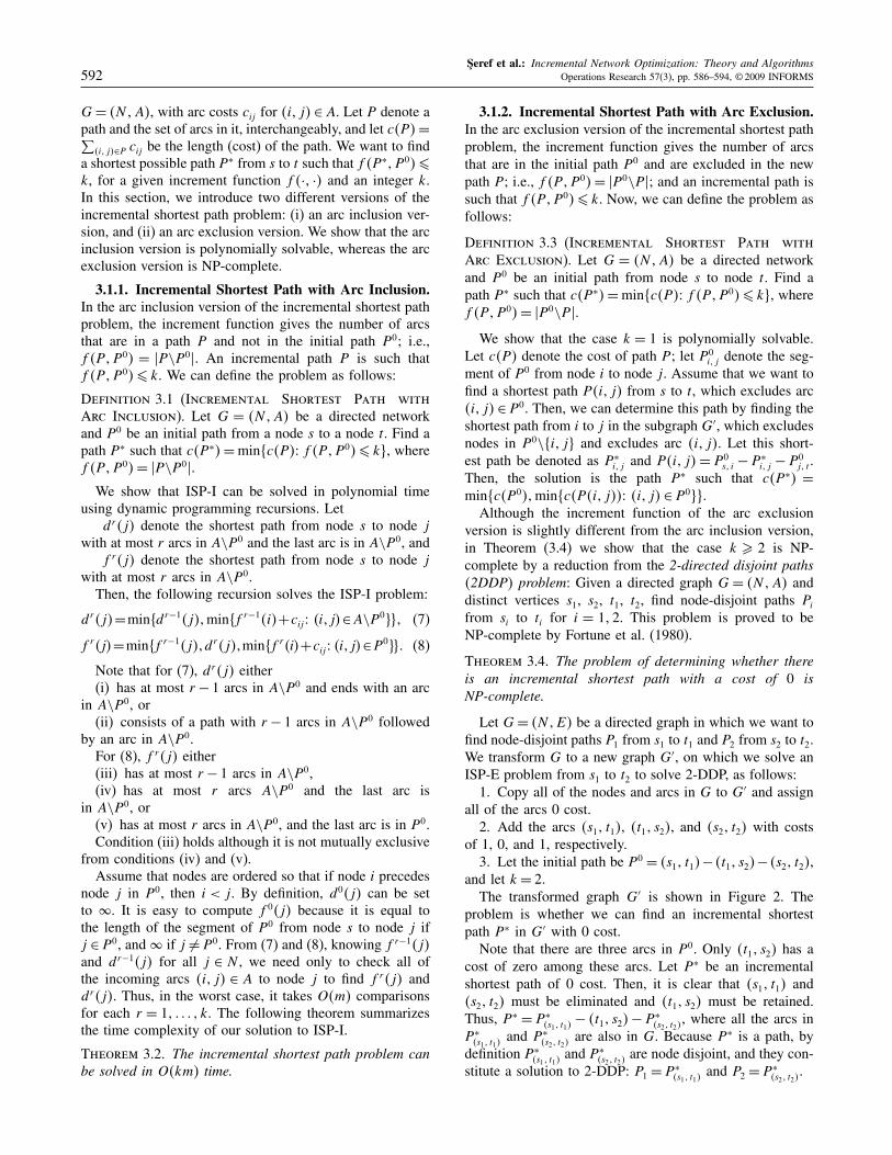
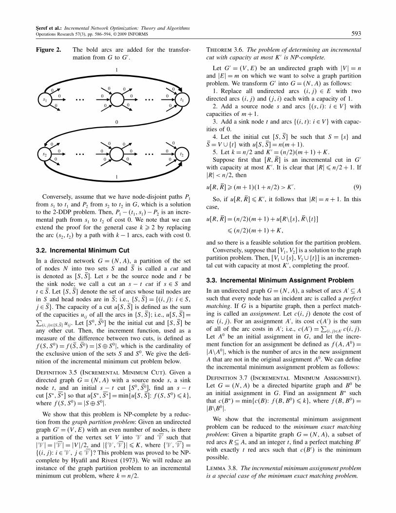
Let G= �N �E� be a directed graph in which we want tofind node-disjoint paths P1 from s1 to t1 and P2 from s2 to t2.We transform G to a new graph G′, on which we solve anISP-E problem from s1 to t2 to solve 2-DDP, as follows:1. Copy all of the nodes and arcs in G to G′ and assign

all of the arcs 0 cost.2. Add the arcs �s1� t1�, �t1� s2�, and �s2� t2� with costs

of 1, 0, and 1, respectively.3. Let the initial path be P 0 = �s1� t1�− �t1� s2�− �s2� t2�,

and let k = 2.The transformed graph G′ is shown in Figure 2. The

problem is whether we can find an incremental shortestpath P ∗ in G′ with 0 cost.Note that there are three arcs in P 0. Only �t1� s2� has a

cost of zero among these arcs. Let P ∗ be an incrementalshortest path of 0 cost. Then, it is clear that �s1� t1� and�s2� t2� must be eliminated and �t1� s2� must be retained.Thus, P ∗ = P ∗

�s1� t1�− �t1� s2�− P ∗

�s2� t2�, where all the arcs in

P ∗�s1� t1�

and P ∗�s2� t2�

are also in G. Because P ∗ is a path, bydefinition P ∗

�s1� t1�and P ∗

�s2� t2�are node disjoint, and they con-

stitute a solution to 2-DDP: P1 = P ∗�s1� t1�

and P2 = P ∗�s2� t2�

.


Figure 2. The bold arcs are added for the transfor-mation from G to G′.

0

0

0 0

0

0

0

0

0 0

0

0

t1

0

0

0

t2

0

0

0

s10

00

s20

0

0

...

...

...

...

1

1

0

Conversely, assume that we have node-disjoint paths P1

from s1 to t1 and P2 from s2 to t2 in G, which is a solutionto the 2-DDP problem. Then, P1− �t1� s1�−P2 is an incre-mental path from s1 to t2 of cost 0. We note that we canextend the proof for the general case k � 2 by replacingthe arc �s2� t2� by a path with k− 1 arcs, each with cost 0.

3.2. Incremental Minimum Cut

In a directed network G = �N �A�, a partition of the setof nodes N into two sets S and �S is called a cut andis denoted as 4S� �S5. Let s be the source node and t bethe sink node; we call a cut an s − t cut if s ∈ S andt ∈ �S. Let S� �S� denote the set of arcs whose tail nodes arein S and head nodes are in �S; i.e., S� �S� = �i� j�� i ∈ S�j ∈ �S�. The capacity of a cut u4S� �S5 is defined as the sumof the capacities uij of all the arcs in S� �S�; i.e., u4S� �S5=∑

�i� j�∈S��S� uij . Let 4S0� �S05 be the initial cut and 4S� �S5 beany other cut. Then, the increment function, used as ameasure of the difference between two cuts, is defined asf �S�S0� = f � �S� �S0� = �S ⊕ S0�, which is the cardinality ofthe exclusive union of the sets S and S0. We give the defi-nition of the incremental minimum cut problem below.

Definition 3.5 (Incremental Minimum Cut). Given adirected graph G = �N �A� with a source node s, a sinknode t, and an initial s − t cut 4S0� �S05, find an s − tcut 4S∗� �S∗5 so that u4S∗� �S∗5=minu4S� �S5� f �S�S0�� k�,where f �S�S0�= �S ⊕ S0�.We show that this problem is NP-complete by a reduc-

tion from the graph partition problem: Given an undirectedgraph G′ = �V �E� with an even number of nodes, is therea partition of the vertex set V into � and �� such that�� = � �� = �V �/2, and �� K, where � � �� =�i� j�� i ∈� � j ∈ �� ? This problem was proved to be NP-complete by Hyafil and Rivest (1973). We will reduce aninstance of the graph partition problem to an incrementalminimum cut problem, where k = n/2.

Theorem 3.6. The problem of determining an incrementalcut with capacity at most K ′ is NP-complete.

Let G′ = �V �E� be an undirected graph with �V � = nand �E� = m on which we want to solve a graph partitionproblem. We transform G′ into G= �N �A� as follows:1. Replace all undirected arcs �i� j� ∈ E with two

directed arcs �i� j� and �j� i� each with a capacity of 1.2. Add a source node s and arcs �s� i�� i ∈ V � with

capacities of m+ 1.3. Add a sink node t and arcs �i� t�� i ∈ V � with capac-

ities of 0.4. Let the initial cut 4S� �S5 be such that S = s� and

�S = V ∪ t� with u4S� �S5= n�m+ 1�.5. Let k = n/2 and K ′ = �n/2��m+ 1�+K.Suppose first that 4R� �R5 is an incremental cut in G′

with capacity at most K ′. It is clear that �R�� n/2+ 1. If�R�< n/2, then

u4R� �R5� �m+ 1��1+ n/2� > K ′� (9)

So, if u4R� �R5 � K ′, it follows that �R� = n + 1. In thiscase,

u4R� �R5= �n/2��m+ 1�+ u4R\s�� R\t�5� �n/2��m+ 1�+K�

and so there is a feasible solution for the partition problem.Conversely, suppose that 4V1� V25 is a solution to the graph

partition problem. Then, 4V1∪ s��V2∪ t�5 is an incremen-tal cut with capacity at most K ′, completing the proof.

3.3. Incremental Minimum Assignment Problem

In an undirected graph G= �N �A�, a subset of arcs A′ ⊆Asuch that every node has an incident arc is called a perfectmatching. If G is a bipartite graph, then a perfect match-ing is called an assignment. Let c�i� j� denote the cost ofarc �i� j�. For an assignment A′, its cost c�A′� is the sumof all of the arc costs in A′; i.e., c�A′� =∑

�i� j�∈A′ c�i� j�.Let A0 be an initial assignment in G, and let the incre-ment function for an assignment be defined as f �A�A0�=�A\A0�, which is the number of arcs in the new assignmentA that are not in the original assignment A0. We can definethe incremental minimum assignment problem as follows:

Definition 3.7 (Incremental Minimum Assignment).Let G = �N �A� be a directed bipartite graph and B0 bean initial assignment in G. Find an assignment B∗ suchthat c�B∗� = minc�B�� f �B�B0� � k�, where f �B�B0� =�B\B0�.We show that the incremental minimum assignment

problem can be reduced to the minimum exact matchingproblem: Given a bipartite graph G = �N �A�, a subset ofred arcs R⊆A, and an integer t, find a perfect matching Bt

with exactly t red arcs such that c�Bt� is the minimumpossible.

Lemma 3.8. The incremental minimum assignment problemis a special case of the minimum exact matching problem.


In the incremental minimum assignment problem, thearcs that are not in the initial assignment B0 can be con-sidered as the set of red arcs; i.e., R = A\B0. If we add nadditional arcs that are copies of arcs in A0, then we mayassume without generality that the optimum solution B∗ hasf �B∗�B0�= k because we can replace arcs of A0 with theircopies and increment f �B∗�A0�. We can find a solution tothe incremental minimum assignment problem by solvingthe minimum exact matching problem for each t.The minimum exact matching problem is solved by

Mulmuley et al. (1987) in random polynomial time if thedata are encoded in unary or if there is an upper bound onthe cost coefficients that is polynomial in n.We note that if we measured the increment function by

arc exclusion, there would be no difference: For any twoassignments A and A0, �A\A0� = �A0\A�.

4. ConclusionIn this paper, we study six incremental network optimiza-tion problems. We show that, using Lagrangian relaxationand approximate binary search, we can efficiently solvethe incremental minimum spanning tree problem. We alsoshow that the incremental minimum cost flow and incre-mental maximum flow problems are polynomial time solv-able using Lagrangian relaxation. We study two versionsof the incremental shortest path problem. The arc inclu-sion version, which limits the number of new arcs, can besolved very efficiently, whereas the arc exclusion version,which limits the number of arcs excluded from the origi-nal solution, is an NP-complete problem. We show that theincremental minimum cut problem is also NP-complete andthat the incremental minimum assignment problem is a spe-cial case of the minimum exact matching problem, whichcan be solved by a randomized polynomial time algorithm.

AcknowledgmentsThe third author gratefully acknowledges partial supportfrom a National Science Foundation grant and from Officeof Naval Research grant N000140810029.

ReferencesAarts, E., J. K. Lenstra, eds. 1997. Local Search in Combinatorial Opti-

mization, 1st ed. John Wiley & Sons, New York.Adomavicius, G., A. Gupta. 2005. Toward comprehensive real-time bid-

der support in iterative combinatorial auctions. Inform. Systems Res.16(2) 169–185.

Ahuja, R. K., K. Jha, J. Liu. 2007. Solving real-life railroad blockingproblems. Interfaces 37(5) 404–419.

Ahuja, R. K., T. M. Magnanti, J. B. Orlin. 1993. Network Flows� Theory,Algorithms, and Applicatons. Prentice Hall, Upper Saddle River, NJ.

Ahuja, R. K., Ö. Ergun, J. B. Orlin, A. P. Punnen. 2002. A survey of verylarge-scale neighborhood search techniques. Discrete Appl. Math.123(1–3) 75–102.

Ahuja, R. K., P. Dewan, M. Jaradat, K. C. Jha, A. Kumar. 2006. Anoptimization-based decision support system for train scheduling.Technical report, Innovative Scheduling, Gainesville, FL.

Brucker, P. 1985. Parametric programming and circulation problemswith one additional linear constraint. H. Noltemeier, ed. Proc.WG’85, Workshop on Graph-Theoretic Concepts in Computer Sci-ence, Wurzburg, Germany, 12–21.

Chazelle, B. 2000. A minimum spanning tree algorithm with inverse-Ackermann type complexity. J. ACM 47(6) 1028–1047.

Dimitromanolakis, A. 2002. An analysis of the Golomb ruler and theSidon set problems, and determination of large near-optimal Golombrulers. Master’s thesis, Department of Electronic and Computer Engi-neering, Technical University of Crete, Crete, Greece.

Dos Santos, B. L., M. L. Bariff. 1988. A study of user interface aidsfor model-oriented decision support systems. Management Sci. 34(4)461–468.

Fortune, S., J. Hopcroft, J. Wyllie. 1980. The directed homeomorphismproblem. Theoretical Comput. Sci. 10 111–121.

Higgins, P. G. 1995. Interactive job-shop scheduling: How to combineoperations research heuristics with human abilities. 6th Internat.Conf. Manufacturing Engrg., Institution of Engineers, Melbourne,Victoria, Australia, 293–302.

Holland, J. H. 1975. Adaptation in Natural and Artificial Systems� AnIntroductory Analysis with Applications to Biology, Control, and Arti-ficial Intelligence. University of Michigan Press, Ann Arbor, MI.

Hyafil, L., R. L. Rivest. 1973. Graph partitioning and constructing optimaldecision trees are polynomial complete problems. Report 33, IRIALaboria, Rocquencourt, France.

Li, G., S. Rajagopalan. 1998. Process improvement, quality, and learningeffects. Management Sci. 44(11) 1517–1532.

Little, J. D. C. 1970. Models and managers: The concept of a decisioncalculus. Management Sci. 16 B466–B485.

Mulmuley, K., U. V. Vazirani, V. V. Vazirani. 1987. Matching is as easyas matrix inversion. Combinatorica 7(1) 105–113.

Regan, P. J. 2006. Professional decision modeling: Practitioner as profes-sor. Interfaces 36(2) 142–149.

Vaidyanathan, B., R. K. Ahuja, K. C. Jha. 2008. Real-life locomotiveplanning: New formulations and computational results. Transporta-tion Res. B 42(2) 147–168.

Vaidyanathan, B., K. C. Jha, R. K. Ahuja. 2007. Multicommodity networkflow approach to the railroad crew scheduling problem. IBM J. Res.Development 51(3/4) 325–344.

Wagner, H. M. 1977. Principles of Operations Research. Prentice-Hall,Englewood Cliffs, NJ.

Zangwill, W. I., P. B. Kantor. 1998. Toward a theory of continuous im-provement and the learning curve. Management Sci. 44(7) 910–920.

incremental network optimization: theory and algorithms

Documents