Income and ExpenditureChapter 11(26)

THIRD EDITION

ECONOMICSand

MACROECONOMICSPaul Krugman | Robin Wells

• The nature of the multiplier, which shows how initial changes in spending lead to further changes.

• The meaning of the aggregate consumption function, which shows how disposable income affects consumer spending

• How expected future income and aggregate wealth affect consumer spending

• The determinants of investment spending, and the distinction between planned investment and unplanned inventory investment

• How the inventory adjustment process moves the economy to a new equilibrium after a change in demand

• Why investment spending is considered a leading indicator of the future state of the economy

WHAT YOUWILL LEARN

IN THIS CHAPTER

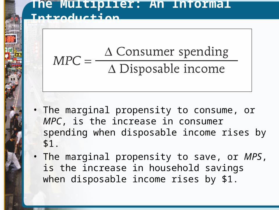
The Multiplier: An Informal Introduction

• The marginal propensity to consume, or MPC, is the increase in consumer spending when disposable income rises by $1.

• The marginal propensity to save, or MPS, is the increase in household savings when disposable income rises by $1.

The Multiplier: An Informal Introduction

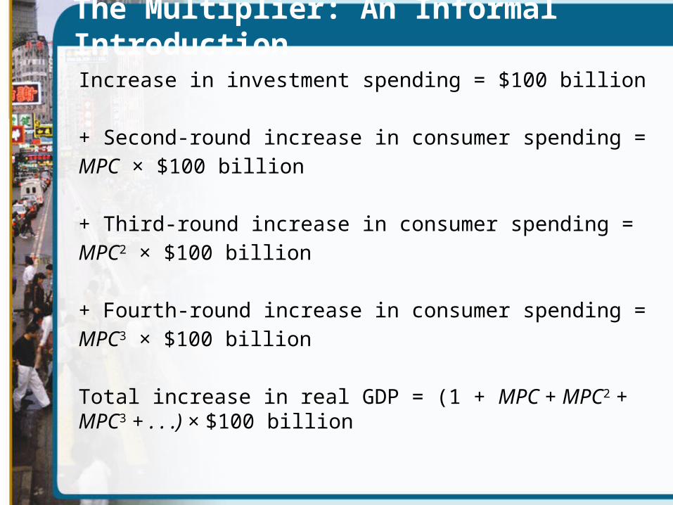
Increase in investment spending = $100 billion

+ Second-round increase in consumer spending = MPC × $100 billion

+ Third-round increase in consumer spending = MPC2 × $100 billion

+ Fourth-round increase in consumer spending = MPC3 × $100 billion

Total increase in real GDP = (1 + MPC + MPC2 + MPC3 + . . .) × $100 billion

The Multiplier: An Informal Introduction

• So the $100 billion increase in investment spending sets off a chain reaction in the economy. The net result of this chain reaction is that a $100 billion increase in investment spending leads to a change in real GDP that is a multiple of the size of that initial change in spending.

• How large is this multiple?

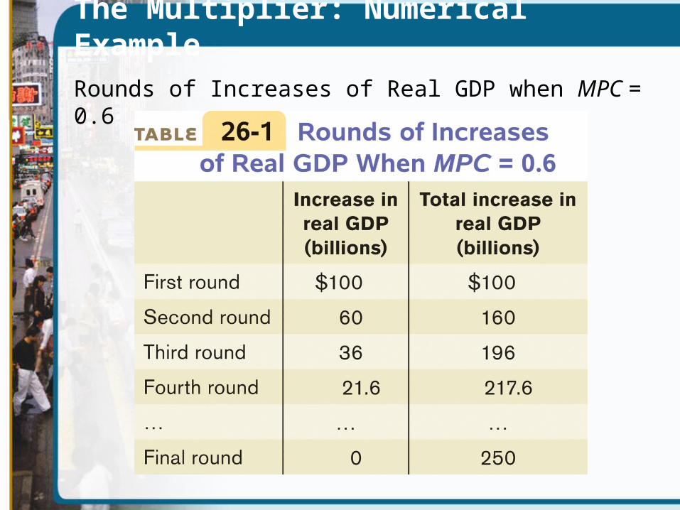
The Multiplier: Numerical Example

Rounds of Increases of Real GDP when MPC = 0.6

The Multiplier: Numerical Example

• In the end, real GDP rises by $250 billion as a consequence of the initial $100 billion rise in investment spending:

• 1/(1 − 0.6) × $100 billion = 2.5 × $100 billion = $250 billion

The Multiplier: An Informal Introduction

• An autonomous change in aggregate spending is an initial change in the desired level of spending by firms, households, or government at a given level of real GDP.

• The multiplier is the ratio of the total change in real GDP caused by an autonomous change in aggregate spending to the size of that autonomous change.

ECONOMICS IN ACTION

The Multiplier and the Great Depression

• The concept of the multiplier was originally devised by economists trying to understand the Great Depression.

• Most economists believe that the slump from 1929 to 1933 was driven by a collapse in investment spending. But as the economy shrank, consumer spending also fell

sharply, multiplying the effect on real GDP.

ECONOMICS IN ACTION

The Multiplier and the Great Depression

• In 1929, government in the United States was very small by modern standards. Taxes were low and major government programs like Social

Security and Medicare had not yet come into being. In the modern U.S. economy, taxes are much higher, and so is

government spending.

• This matters because taxes and some government programs act as automatic stabilizers, reducing the size of the multiplier.

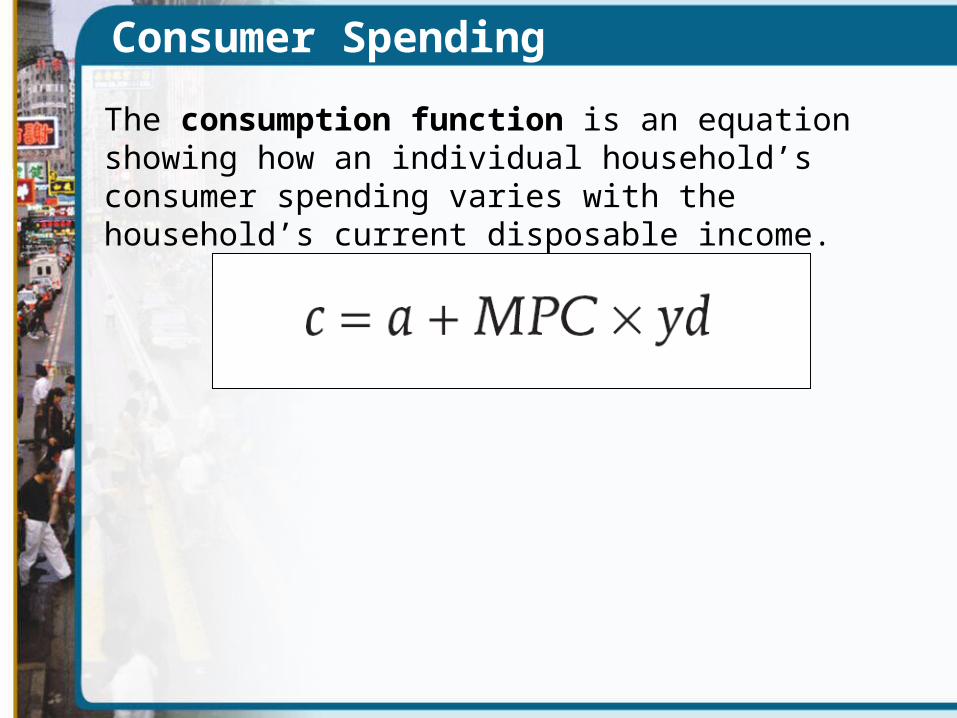
Consumer Spending

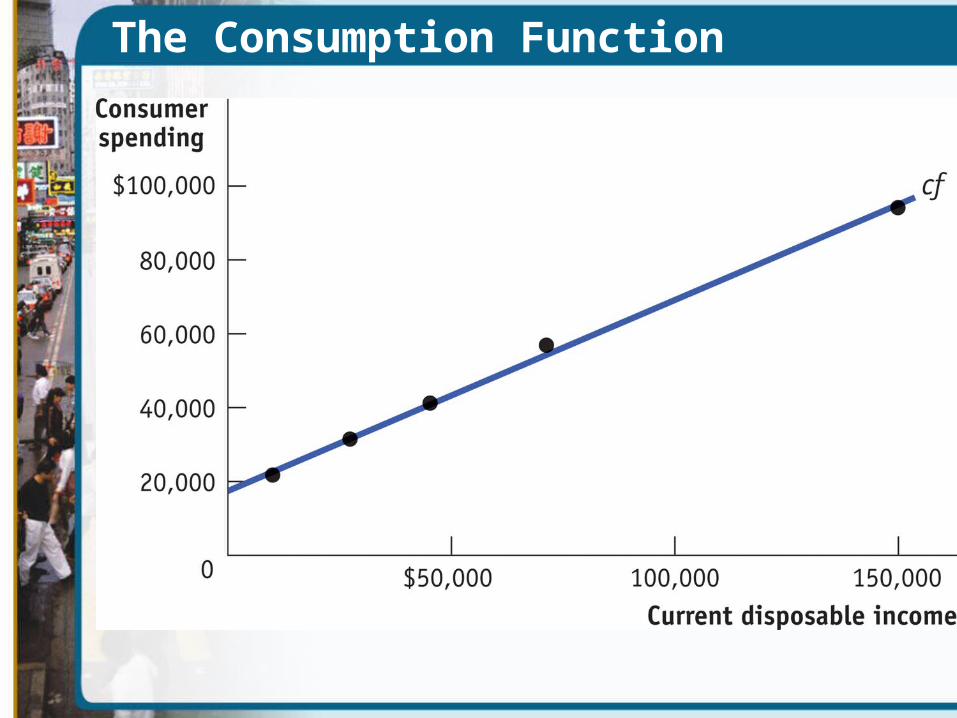
The consumption function is an equation showing how an individual household’s consumer spending varies with the household’s current disposable income.

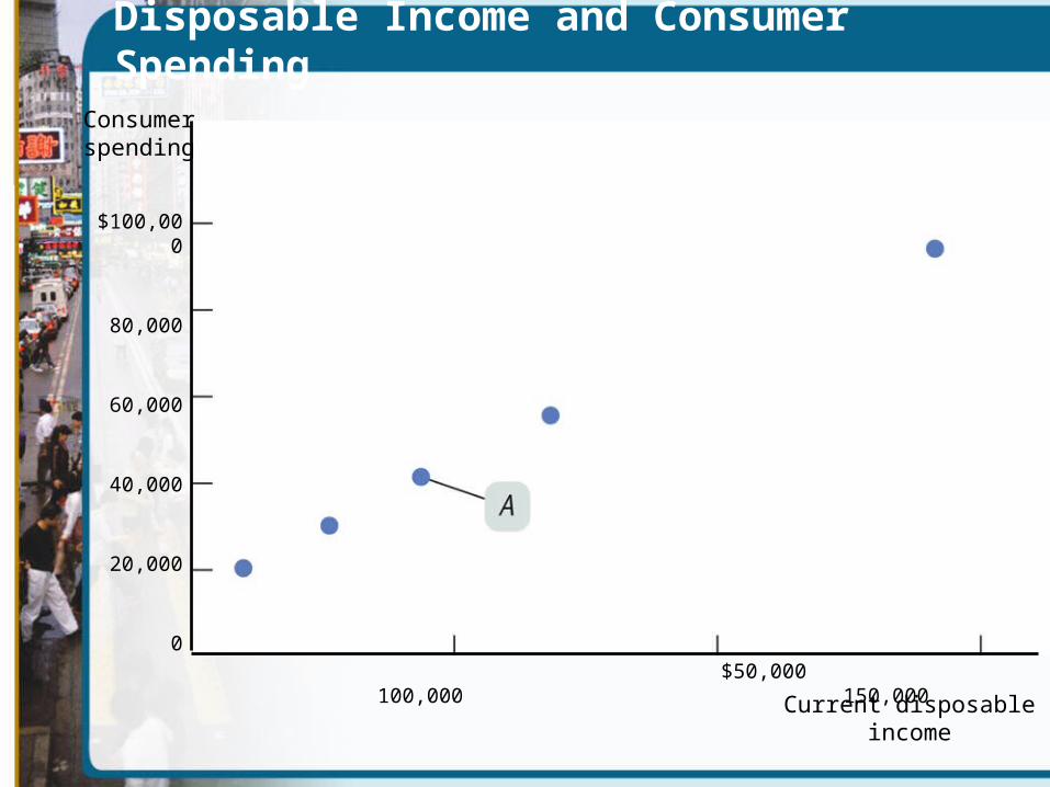
Disposable Income and Consumer Spending

$50,000 100,000 150,000 Current disposable

income

$100,000

80,000

60,000

40,000

20,000

0

Consumer spending

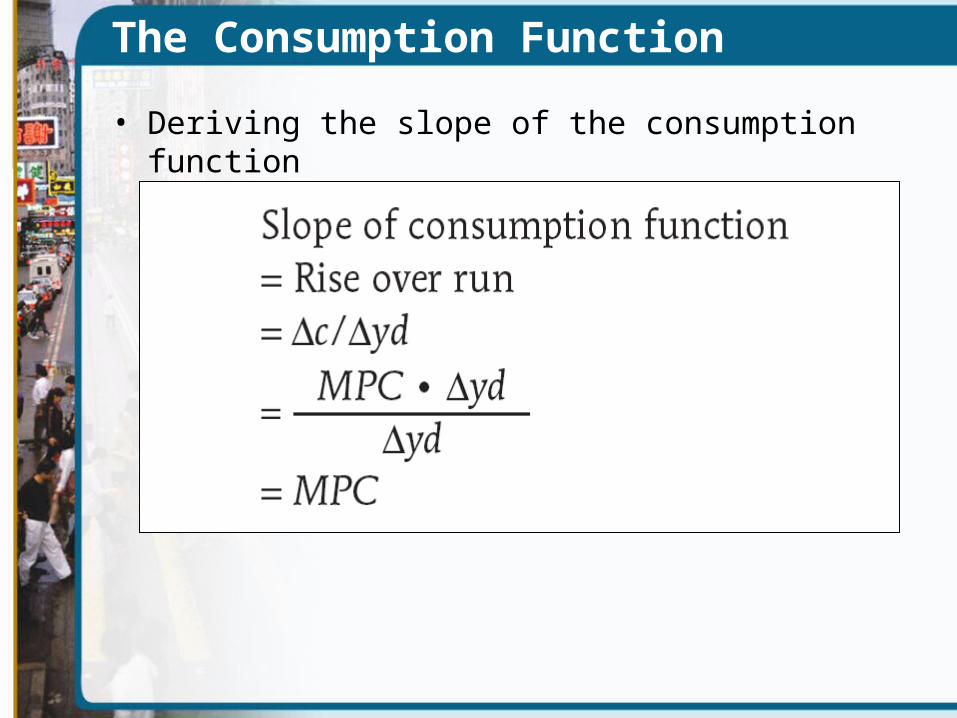
The Consumption Function

The Consumption Function

• Deriving the slope of the consumption function

The Consumption Function

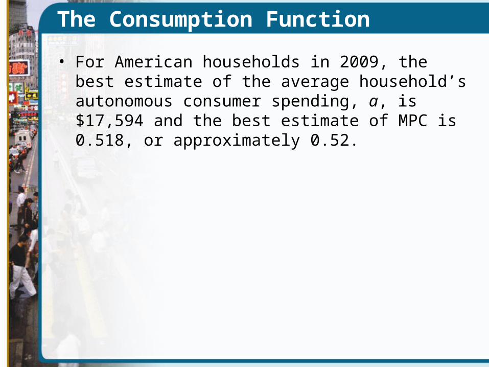
• For American households in 2009, the best estimate of the average household’s autonomous consumer spending, a, is $17,594 and the best estimate of MPC is 0.518, or approximately 0.52.

The Consumption Function

Aggregate Consumption Function

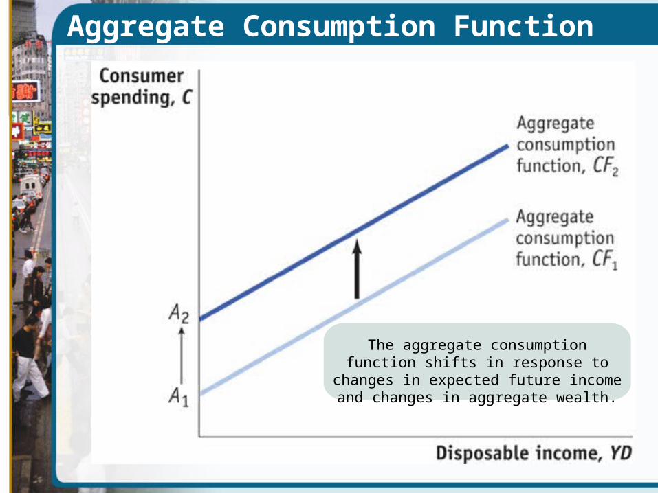
• The aggregate consumption function is the relationship for the economy as a whole between aggregate current disposable income and aggregate consumer spending.

Aggregate Consumption Function

The aggregate consumption function shifts in response to changes in

expected future income and changes in aggregate wealth.

Aggregate Consumption Function

Aggregate Consumption Function

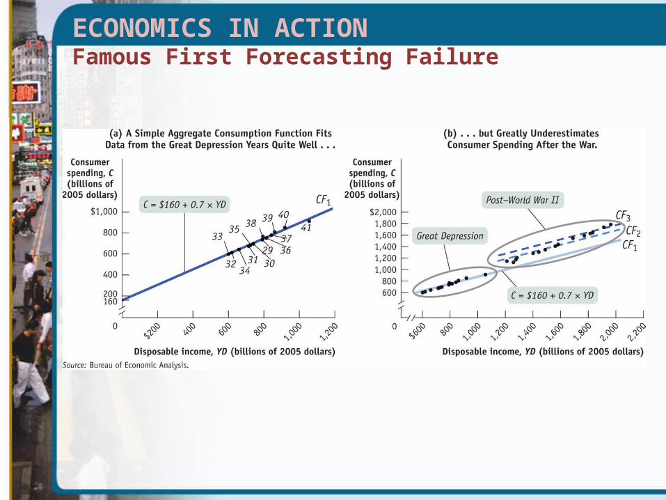
ECONOMICS IN ACTIONFamous First Forecasting Failure

Investment Spending

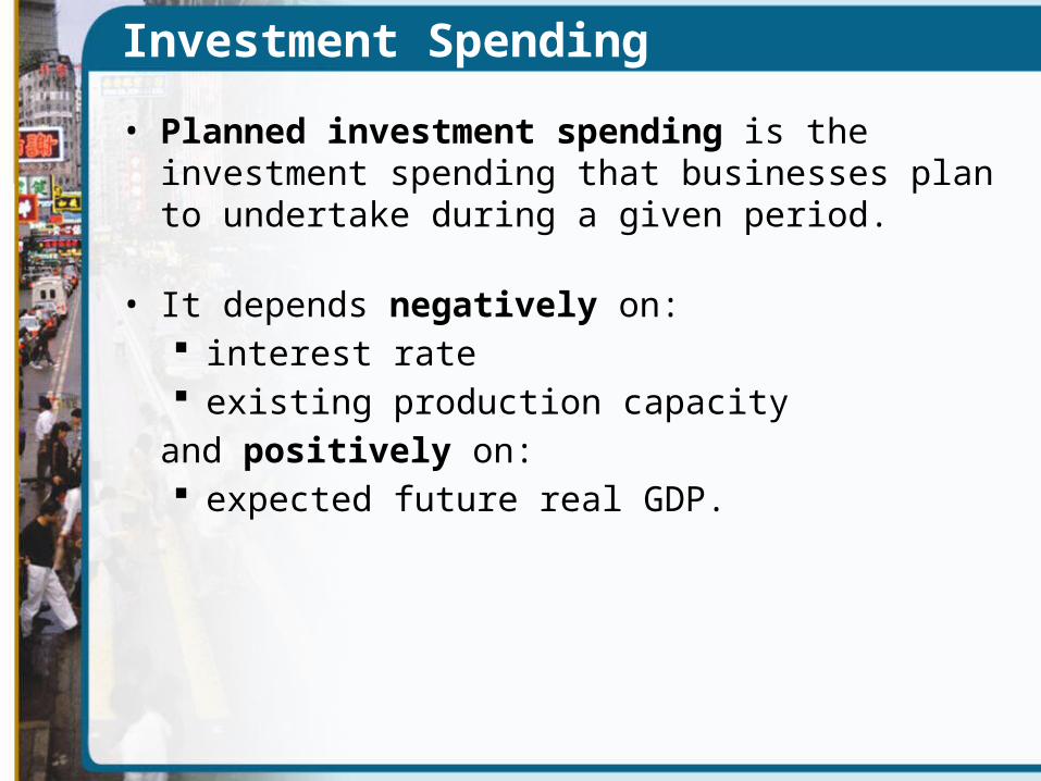
• Planned investment spending is the investment spending that businesses plan to undertake during a given period.

• It depends negatively on: interest rate existing production capacity

and positively on: expected future real GDP.

Investment Spending

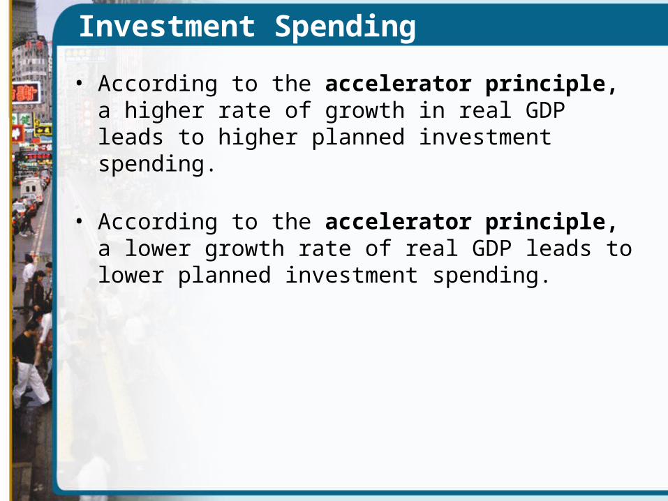
• According to the accelerator principle, a higher rate of growth in real GDP leads to higher planned investment spending.

• According to the accelerator principle, a lower growth rate of real GDP leads to lower planned investment spending.

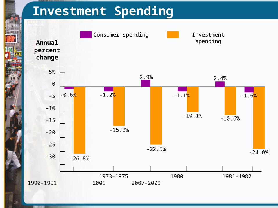
Investment Spending

5%

0

–5

–10

–15

–20

–25

–30

Annualpercentchange

1973–1975 1980 1981–1982 1990–1991 2001 2007-2009

-15.9%

-26.8%

-10.1%

-22.5%

-10.6%

-0.6%

2.4%

-1.1%-1.2%

2.9%

Consumer spending Investment spending

-1.6%

-24.0%

Inventories and Unplanned Investment Spending

• Inventories are stocks of goods held to satisfy future sales.

• Inventory investment is the value of the change in total inventories held in the economy during a given period.

• Unplanned inventory investment occurs when actual sales are more or less than businesses expected, leading to unplanned changes in inventories.

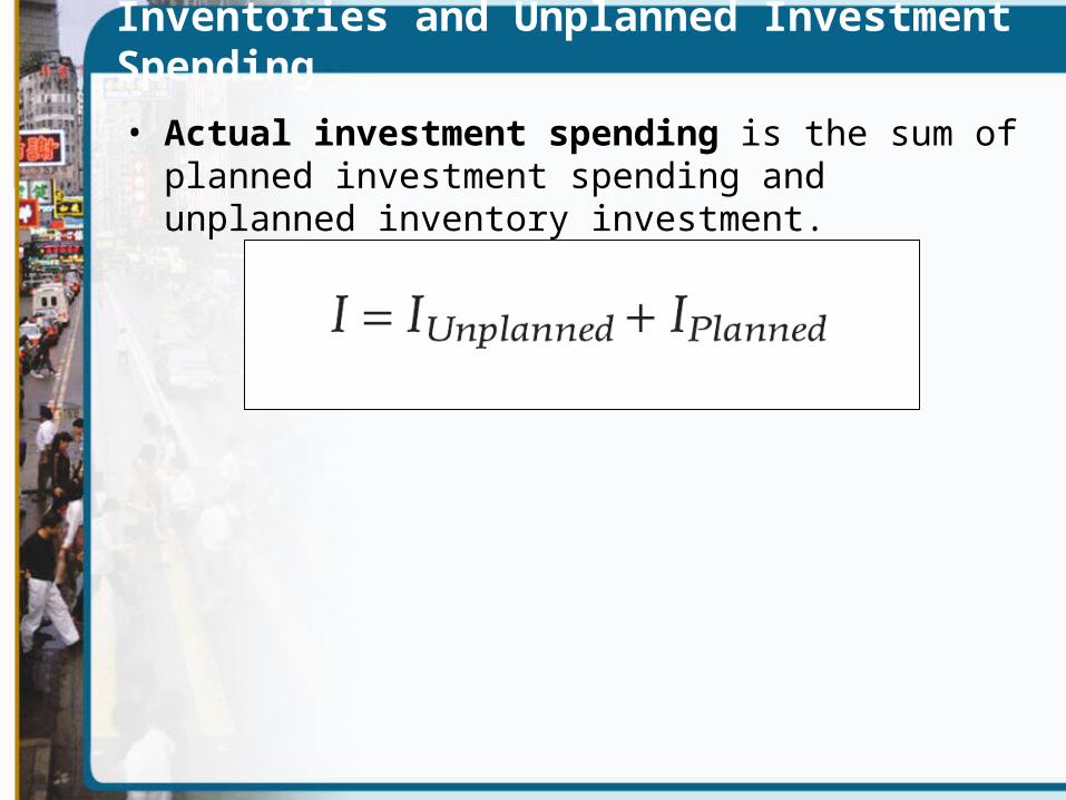
Inventories and Unplanned Investment Spending

• Actual investment spending is the sum of planned investment spending and unplanned inventory investment.

ECONOMICS IN ACTION

Interest Rates and the U.S. Housing Boom

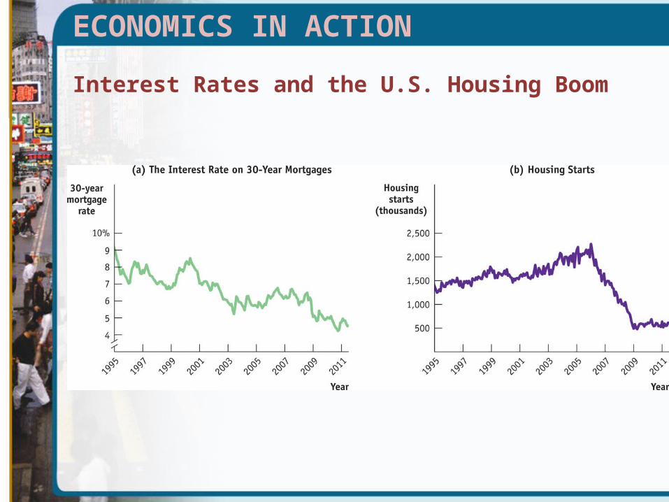
• The Fed cut mortgage rates in response to the 2001 recession and continued cutting them into 2003 out of concern that the economy’s recovery was too weak to generate sustained job growth.

• The low interest rates led to a large increase in residential investment spending, reflected in a surge of housing starts. Unfortunately, the housing boom eventually turned into too

much of a good thing.

ECONOMICS IN ACTION

Interest Rates and the U.S. Housing Boom

• By 2006, it was clear that the U.S. housing market was experiencing a bubble. People were buying housing based on unrealistic expectations

about future price increases. When the bubble burst, housing—and the U.S. economy—took a fall.

ECONOMICS IN ACTION

Interest Rates and the U.S. Housing Boom

Income-Expenditure Model

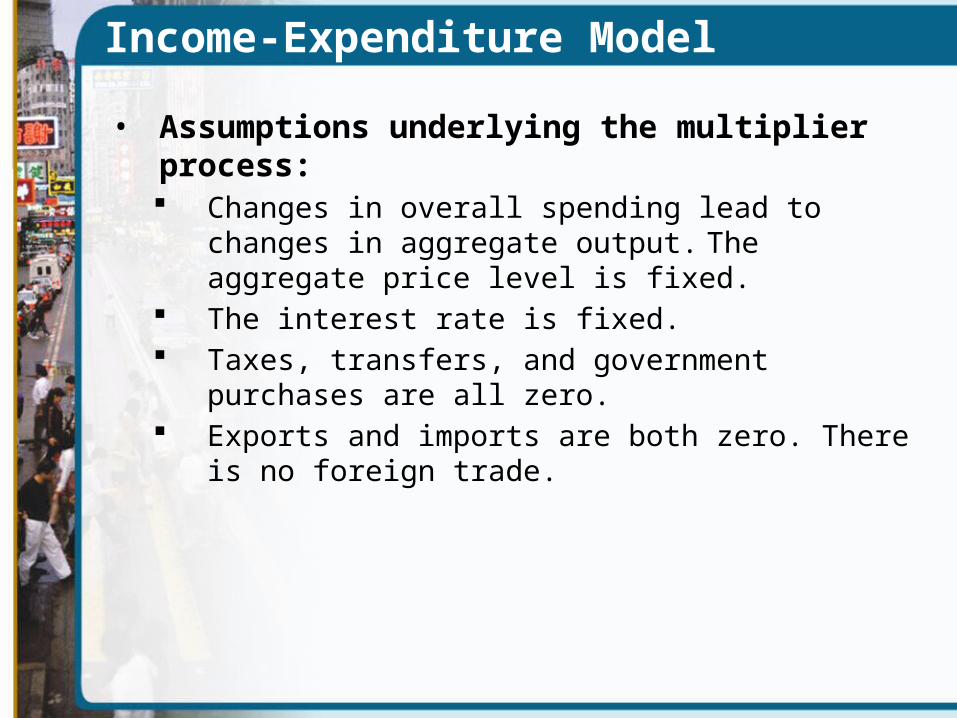
• Assumptions underlying the multiplier process: Changes in overall spending lead to changes in aggregate

output. The aggregate price level is fixed. The interest rate is fixed. Taxes, transfers, and government purchases are all zero. Exports and imports are both zero. There is no foreign

trade.

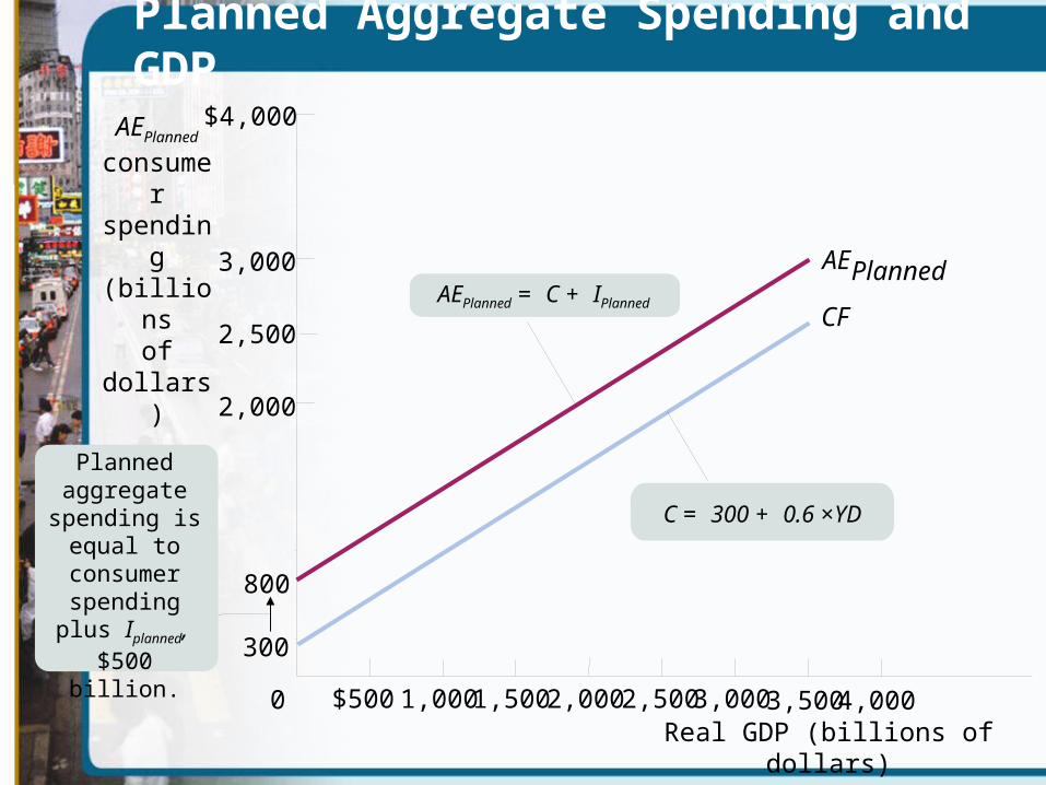
Planned Aggregate Spending and GDP

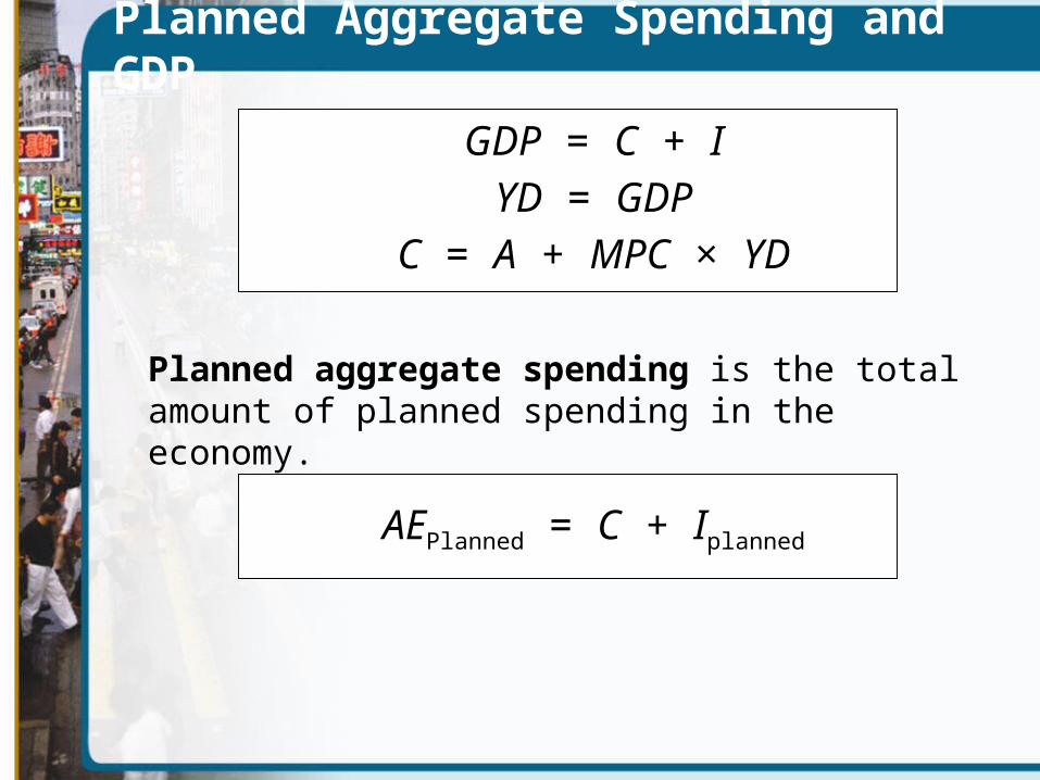
Planned aggregate spending is the total amount of planned spending in the economy.

GDP = C + IYD = GDP

C = A + MPC × YD

AEPlanned = C + Iplanned

AEPlanned

CF

0

300

2,0002,500 3,5003,0001,5001,000$500

800

$4,000

3,000

2,500

2,000

4,000

AEPlanned

consumer

spending(billions

of dollars)

Real GDP (billions of dollars)

Planned aggregate spending is

equal to consumer

spending plus Iplanned,

$500 billion.

AEPlanned = C + IPlanned

C = 300 + 0.6 ×YD

Planned Aggregate Spending and GDP

Income–Expenditure Equilibrium

• The economy is in income–expenditure equilibrium when aggregate output, measured by real GDP, is equal to planned aggregate spending.

• Income–expenditure equilibrium GDP is the level of real GDP at which real GDP equals planned aggregate spending.

Income–Expenditure Equilibrium

• When planned aggregate spending is larger than Y*, unplanned inventory investment is negative; there is an unanticipated reduction in inventories and firms increase production.

• When planned aggregate spending is less than Y*, unplanned inventory investment is positive; there is an unanticipated increase in inventories and firms reduce production.

Y*

E

2,0002,500 3,5003,0001,5001,000$500

800

$4,000

3,000

2,000

1,000

04,000

1,400

Real GDP (billions of dollars)

Plannedaggregatespending,AEPlanned

(billions of

dollars)

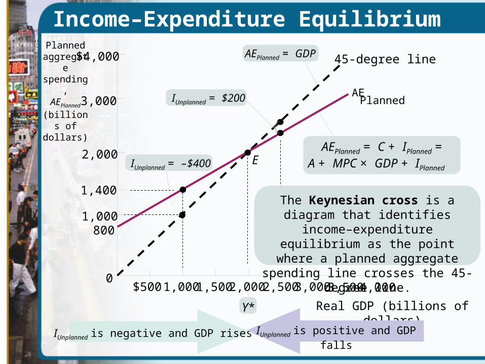
IUnplanned is negative and GDP rises

IUnplanned = –$400

IUnplanned is positive and GDP falls

IUnplanned = $200

AEPlanned = GDP

AEPlanned = C + IPlanned =A + MPC × GDP + IPlanned

AEPlanned

45-degree line

The Keynesian cross is a diagram that identifies income–expenditure equilibrium as the point where a planned aggregate spending line

crosses the 45-degree line.

Income–Expenditure Equilibrium

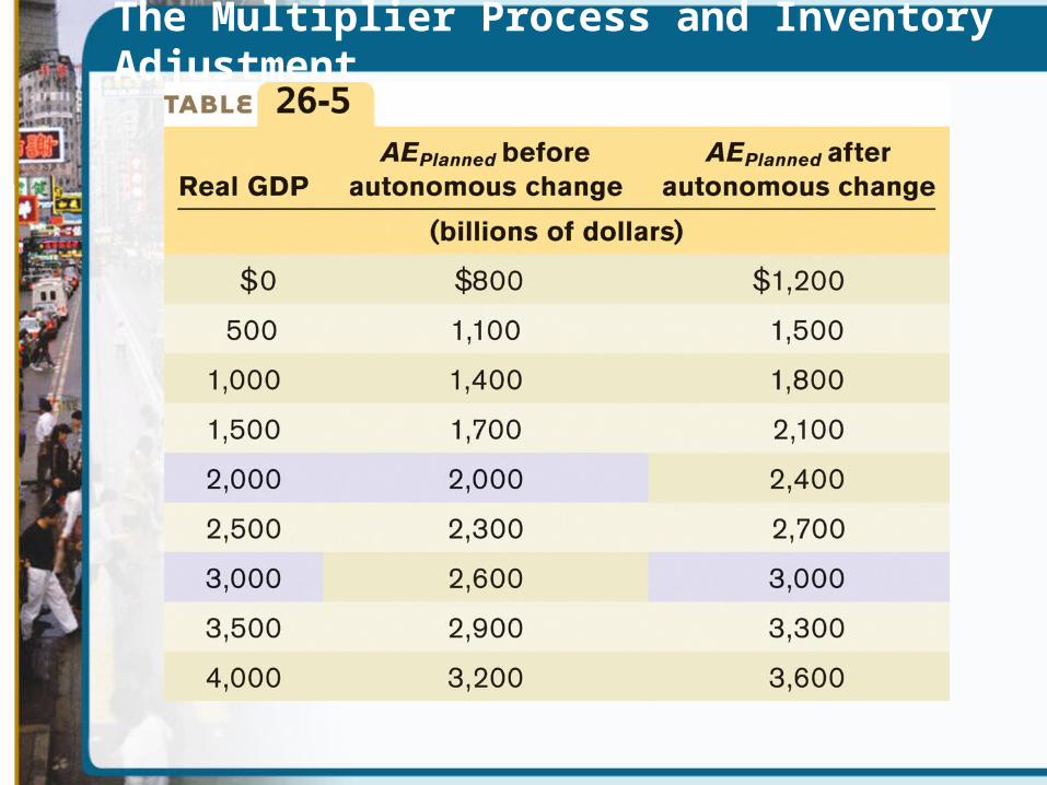
The Multiplier Process and Inventory Adjustment

Y2*

E2

AEPlanned afterautonomous

changeAEPlanned2

2,400X

IUnplanned = –$400

1,200Autonomous increase of $400 in aggregate spending

AEPlanned1

800

0

$4,000

3,000

2,000

2,000 2,500 3,500 4,0003,0001,5001,000$500

E1

Y1*

Plannedaggregat

espending

,AEPlanned

(billions of

dollars)

Real GDP (billions of dollars)

AEPlanned beforeautonomous

change

ΔY* = Multiplier × ΔAAEPlanned

= 1 / (1 – MPC) × ΔAAEPlanned

The Multiplier

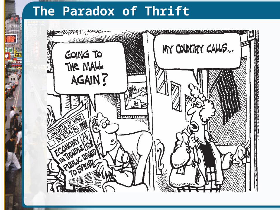
The Paradox of Thrift

• In the paradox of thrift, households and producers cut their spending in anticipation of future tough economic times.

• These actions depress the economy, leaving households and producers worse off than if they hadn’t acted virtuously to prepare for tough times.

• It is called a paradox because what’s usually “good” (saving to provide for your family in hard times) is “bad” (because it can make everyone worse off).

The Paradox of Thrift

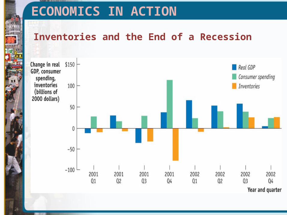
ECONOMICS IN ACTION

Inventories and the End of a Recession

Summary

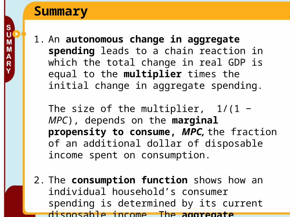
1. An autonomous change in aggregate spending leads to a chain reaction in which the total change in real GDP is equal to the multiplier times the initial change in aggregate spending.

The size of the multiplier, 1/(1 − MPC), depends on the marginal propensity to consume, MPC, the fraction of an additional dollar of disposable income spent on consumption.

2. The consumption function shows how an individual household’s consumer spending is determined by its current disposable income. The aggregate consumption function shows the relationship for the entire economy.

Summary

3. Planned investment spending depends negatively on the interest rate and on existing production capacity; it depends positively on expected future real GDP.

The accelerator principle says that investment spending is greatly influenced by the expected growth rate of real GDP.

Summary

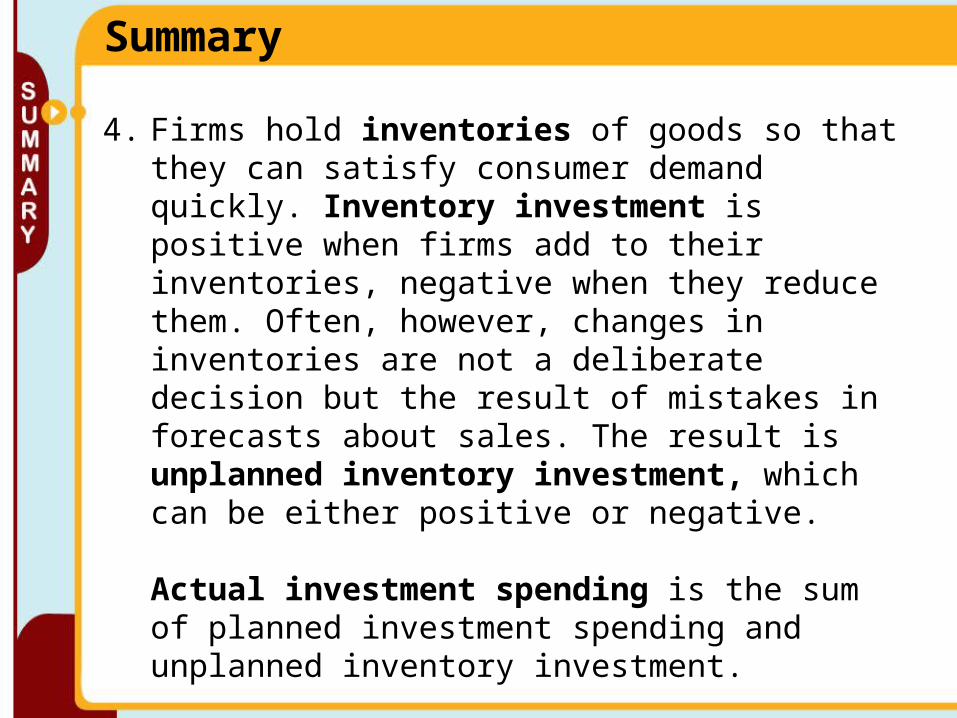
4. Firms hold inventories of goods so that they can satisfy consumer demand quickly. Inventory investment is positive when firms add to their inventories, negative when they reduce them. Often, however, changes in inventories are not a deliberate decision but the result of mistakes in forecasts about sales. The result is unplanned inventory investment, which can be either positive or negative.

Actual investment spending is the sum of planned investment spending and unplanned inventory investment.

Summary

5. In income–expenditure equilibrium, planned aggregate spending, which in a simplified model with no government and no trade is the sum of consumer spending and planned investment spending, is equal to real GDP.

At the income–expenditure equilibrium GDP, or Y*, unplanned inventory investment is zero.

The Keynesian cross shows how the economy self-adjusts to income–expenditure equilibrium through inventory adjustments

Summary

6. After an autonomous change in planned aggregate spending, the inventory adjustment process moves the economy to a new income–expenditure equilibrium.

The change in income–expenditure equilibrium GDP arising from an autonomous change in spending is equal to (1/(1 − MPC)) × Δ AAEPlanned.

• Marginal propensity to consume (MPC)

• Marginal propensity to save (MPS)

• Autonomous change in aggregate spending

• Multiplier• Consumption function• Aggregate consumption

function• Planned investment

spending• Accelerator principle

• Inventories• Inventory investment• Unplanned inventory

investment• Actual investment spending• Planned aggregate spending• Income–expenditure

equilibrium• Income–expenditure

equilibrium GDP• Keynesian cross

Key Terms