in-vivo confocal evaluation of corneal nerves in patients
TRANSCRIPT

In-Vivo Confocal Evaluation of Corneal Nerves in Patients with Diabetic Neuropathy
BY
Nilesh Raval
A thesis submitted in fulfillment of the Honors Biophysics Undergraduate Program in the College of Literature, Science, and the Arts
at the
University of Michigan in Ann Arbor
December 20, 2013

Biophysics Undergraduate Honors Thesis Raval 1
Table of Contents
Abstract…………………………………………………………………………………… 2
Introduction……………………………………………………………………………….. 3-4
Background……………………………………………………………………………….. 5-15
Materials/Methods………………………………………………………………………… 16-18
Results/Discussion………………………………………………………………………… 19-32
Conclusion………………………………………………………………………………… 33-34
Acknowledgements……………………………………………………………………….. 35
References…………………………………………………………………………………. 36-38

Biophysics Undergraduate Honors Thesis Raval 2
Abstract
Purpose: The objective of the first part of this study was to determine if the corneal nerve
parameters of mean nerve count, total nerve length, percent primary nerve character, and
tortuosity of nerves in the subbasal nerve plexus varied amongst three groups of patients: those
with severe diabetic neuropathy, those with diabetes and mild to no clinical evidence of
neuropathy, and a healthy control group. The second part of this study focused on correlating
nerve tortuosity values with mean nerve count, total nerve length, and primary nerve character.
Methods: Confocal data for patients with severe diabetic neuropathy (n = 7), diabetes and mild or
no neuropathy (n = 15), and healthy controls (n = 9) were collected with the Heidelberg Retina
Tomograph confocal microscope and analyzed using NeuronJ and CCMetric. Image analysis
included determining the mean nerve count, total nerve length, percentage of primary nerves, and
tortuosity values for each scan. Analysis of variance, Tukey’s post-hoc test, and the Pearson
Coefficient of Determination were used as tools for statistical analysis.
Results: There was a statistically significant difference (p < 0.05) in the mean nerve count
between the healthy control group and the severe neuropathy group. The healthy control group
expressed a strong linear relationships when comparing tortuosity with mean nerve count (R2 =
0.77) and mean nerve length (R2 = 0.64), while the severe neuropathy group expressed its lowest
values of mean nerve count and total nerve length at the highest and lowest tortuosity values.
Conclusions: The results support the hypothesis that corneal nerves, as imaged by confocal
microscopy, correlate to, and can be used as diagnostic markers for, systemic diabetic
neuropathy. A larger patient sample size will increase confidence and reliability of the data, and
an automated MATLAB script currently being developed will speed up the analysis process.

Biophysics Undergraduate Honors Thesis Raval 3
Introduction
Over 25 million people in the United States suffer from diabetes, and about 60-70% of diabetics
express mild to severe forms of neuropathy [1]. In the past, the only method of directly
examining the peripheral nerves was to conduct skin or nerve biopsies, which were
uncomfortable and invasive. The benefit of using ophthalmic markers for early detection of
diabetic peripheral neuropathy is that the procedure is non-invasive, cost-efficient, and clinically
accessible. The first objective of this research is to compare the characteristics of corneal nerves
– mean count, mean length, primary nerve character, and tortuosity – in patients with diabetes
and severe neuropathy, diabetes and mild to no clinical evidence of neuropathy, and a healthy
control group. The second objective is to determine how nerve tortuosity, a parameter that has
not been studied extensively in the field, correlates with nerve count, length, and character. The
ultimate goal of this study is to utilize the results as a quantitative diagnostic that can indicate the
presence of diabetic neuropathy in patients before full expression of clinical symptoms of the
disease arises.
The cornea can be easily examined in an outpatient setting using corneal confocal microscopy,
an in-vivo procedure that involves shining a pinpoint laser into the patient’s eye, progressively
scanning through the layers of the cornea, and transmitting the scans to a digital imaging
program to quantify the data. The presence of significant differences between groups of patients
could hint at a pathophysiological mechanism relating the systemic condition of diabetes to the
status of the corneal nerves. If significant correlations between diabetic neuropathy and corneal
nerve parameters can be quantified, a model for the quantitative relationship between the severity
of diabetic neuropathy and corneal nerve parameters can be established. This diagnostic model

Biophysics Undergraduate Honors Thesis Raval 4
could be utilized during routine doctor appointments or at regular eye exams to non-invasively
test for early detection of diabetic neuropathy.
It is hypothesized that corneal nerves can be used as effective diagnostic markers for diabetic
peripheral neuropathy, and that increased severity of neuropathy will correlate with lower nerve
counts and lower total nerve lengths due to greater nerve damage in the cornea. It is also
hypothesized that increased neuropathy will correlate with lower tortuosity values and a higher
percentage of primary nerve character relative to secondary nerve character, due to the
neuropathic destruction of the more tortuous secondary nerve branches that disrupts nerve-to-
nerve communication. Finally, it is hypothesized that strong correlations will exist between
tortuosity, nerve count, and nerve length in healthy patients but will not exist in neuropathy
patients, as increased nerve damage may reduce the ability of the nerves to sense their
surroundings and adapt to the presence of neighboring nerves by becoming more tortuous and
compact.

Biophysics Undergraduate Honors Thesis Raval 5
Background
The cornea is the outermost layer of the front of the eye [2]. Completely transparent, its purpose
is to refract light onto the retina in the posterior chamber of the eye. The human cornea is
comprised of five major layers: the epithelium, Bowman’s layer, the stroma, Descemet’s
membrane, and the endothelium. The epithelium is located on the outside of the cornea and
makes up approximately 10% of the cornea’s overall thickness [2]. The main functions of the
epithelium are to protect the inner layers of the cornea from external debris such as dust particles
and bacteria, and to provide a surface that is capable of absorbing the oxygen and cellular
nutrients of tears and transmitting these nutrients to the inner layers. The bottom layer of the
epithelium, the basement membrane, serves as the anchor for epithelial cells.
Directly beneath the basement membrane lies Bowman’s layer, an 8-14 µm thick, acellular layer
composed of collagen [3]. The exact function of Bowman’s layer has yet to be discovered, but it
has been hypothesized that proper functioning of the human cornea is not dependent on this
layer, as patients who have undergone excimer laser photorefractive keratectomy to remove
Bowman’s layer have not experienced any adverse effects [3,4]. The third layer, the stroma,
accounts for 90% of the entire thickness of the cornea, and it is mainly comprised of water
(~78%) and collagen (~16%) [2]. Stromal collagen is especially important for the maintenance
of corneal structure, strength, and elasticity [2]. Descemet’s membrane, a thin sheet of collagen
fibers, lies directly behind the posterior stroma and serves as a protection against injury and
infection. The innermost layer of the cornea, the endothelium, is responsible for pumping out the
excess fluid that leaks into the stroma from inside the eye, thereby safeguarding against edema
and potential blindness [2].

Biophysics Undergraduate Honors Thesis Raval 6
Between the basal epithelium and Bowman’s layer lies the subbasal, or subepithelial, nerve
plexus, the corneal region responsible for epithelial innervation [5]. The subepithelial region of
the human cornea contains a radiating pattern of bundles of nerve fibers that originate from
stromal nerves and pass through small openings in Bowman’s layer, converging in spiral-like
patterns about 1-2 mm away from the corneal apex, the outermost point of the cornea [6]. The
terminal endings of these nerve fibers reach the epithelial layer but are too small to be seen with
contemporary confocal technology [6]. The nerve plexus consists of highly dense sensory and
autonomic nerve networks, the former of which constitute the ophthalmic branch of the
Figure 1: The five primary layers of the human cornea: epithelium, Bowman’s membrane, stroma, Descemet’s membrane, and endothelium [2].

Biophysics Undergraduate Honors Thesis Raval 7
trigeminal nerve [7]. Mechanical, thermal and chemical stimulation of these sensory nerves is
the primary cause of pain in the human eye [7]. The autonomic network contains both
sympathetic fibers, which are derived from the superior cervical ganglion, and parasympathetic
fibers, which are derived from the ciliary ganglion [7]. The high density of nerve endings in the
cornea is derived from the posterior ciliary nerves, and the cornea is approximately 100 times
more sensitive than the neighboring conjunctiva [8]. If these nerve endings are destroyed, the
cells of the epithelial layer will swell and produce basal lamina, which inhibits mitosis and
directly causes apoptosis of epithelial cells [8].
Figure 2: Subbasal nerve plexus, immediately anterior to Bowman’s layer, as imaged by a confocal microscope [6]. The hyperreflectivity of Bowman’s layer allows for easy characterization and visualization of the nerve plexus [9].
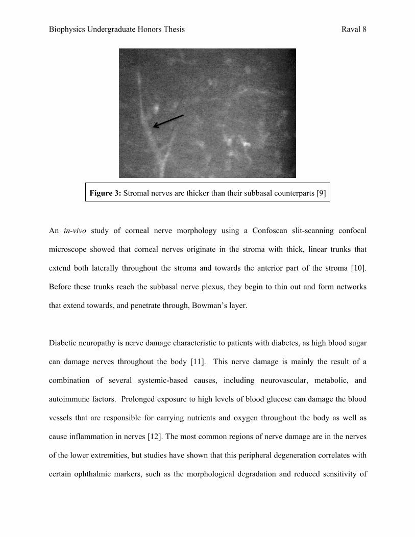
While nerves may also be found in the stromal layer, they are often much thicker than nerves in
the subbasal nerve plexus, and can be differentiated from subbasal nerves as such [9]:
Biophysics Undergraduate Honors Thesis Raval 8
Figure 3: Stromal nerves are thicker than their subbasal counterparts [9]
An in-vivo study of corneal nerve morphology using a Confoscan slit-scanning confocal
microscope showed that corneal nerves originate in the stroma with thick, linear trunks that
extend both laterally throughout the stroma and towards the anterior part of the stroma [10].
Before these trunks reach the subbasal nerve plexus, they begin to thin out and form networks
that extend towards, and penetrate through, Bowman’s layer.
Diabetic neuropathy is nerve damage characteristic to patients with diabetes, as high blood sugar
can damage nerves throughout the body [11]. This nerve damage is mainly the result of a
combination of several systemic-based causes, including neurovascular, metabolic, and
autoimmune factors. Prolonged exposure to high levels of blood glucose can damage the blood
vessels that are responsible for carrying nutrients and oxygen throughout the body as well as
cause inflammation in nerves [12]. The most common regions of nerve damage are in the nerves
of the lower extremities, but studies have shown that this peripheral degeneration correlates with
certain ophthalmic markers, such as the morphological degradation and reduced sensitivity of
Biophysics Undergraduate Honors Thesis Raval 9
corneal nerves, thinning of retinal nerve fibers, and peripheral field loss [13]. This project
focuses on the first marker, corneal nerve degradation, and seeks to correlate key parameters of
this effect, such as nerve count, nerve length, and tortuosity, with severity of diabetic
neuropathy.
In-vivo corneal confocal microscopy is a technique that can be used to obtain a high-resolution
scan of the human cornea. While the slit lamp biomicroscope and ophthalmoscope are also used
by clinicians to observe the cornea, they are unable to do so with high clarity, detail, or
magnification, and so physiological studies of the cornea at the microscopic level have been
limited to in-vitro observations [14]. Light biomicroscopy of corneal layers results in poorly
resolved images, because light is reflected from structures above and below the layer of interest
[9]. For example, if a biomicroscope was used to examine a corneal lesion in the anterior
stromal layer, light reflected from the surrounding layers – the epithelium, the tear film, and even
the endothelium – would cause light contamination and defocus the target layer [9]. The corneal
confocal microscope works on the principle of point illumination, whereby a light source and
camera can be used simultaneously to illuminate and image a specific region of tissue in
coplanar fashion [4]. The resolution of the image captured by a confocal microscope is therefore
much higher than that of a traditional fluorescence microscope, which shines light evenly over an
entire region rather than focusing it on a particular point. Since confocal microscopy only deals
with one point of a sample at a time, the field of view from a single image will be negligibly
small. To account for this potential problem, the confocal microscope “scans” over a small
region of tissue by illuminating it with thousands of tiny points of light, so that a high-resolution,
substantial field-of-view image of the region can be constructed via amalgamation of all of the
Biophysics Undergraduate Honors Thesis Raval 10
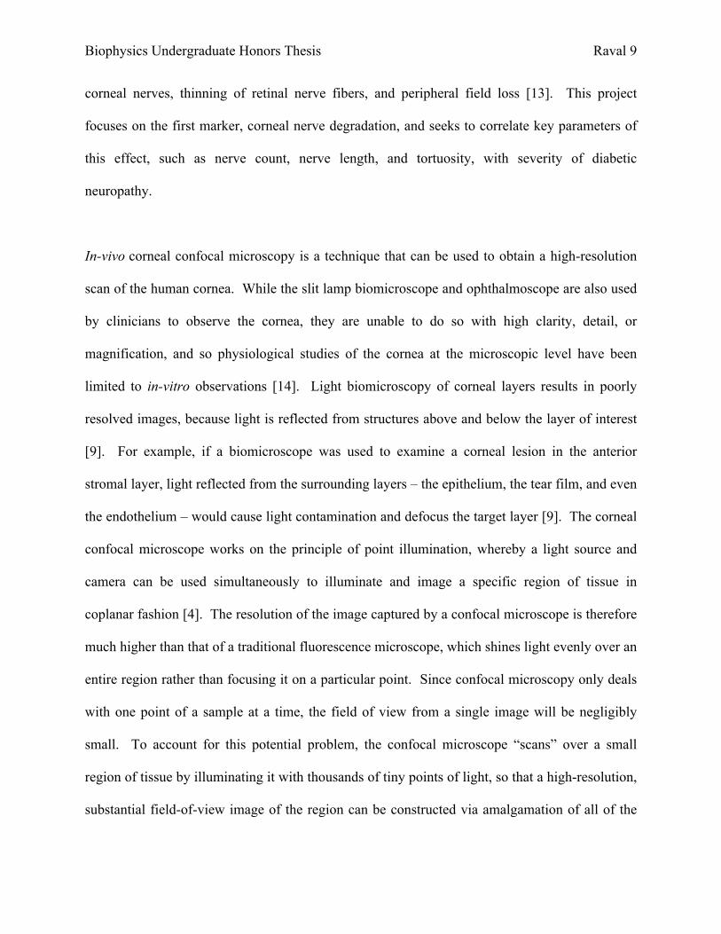
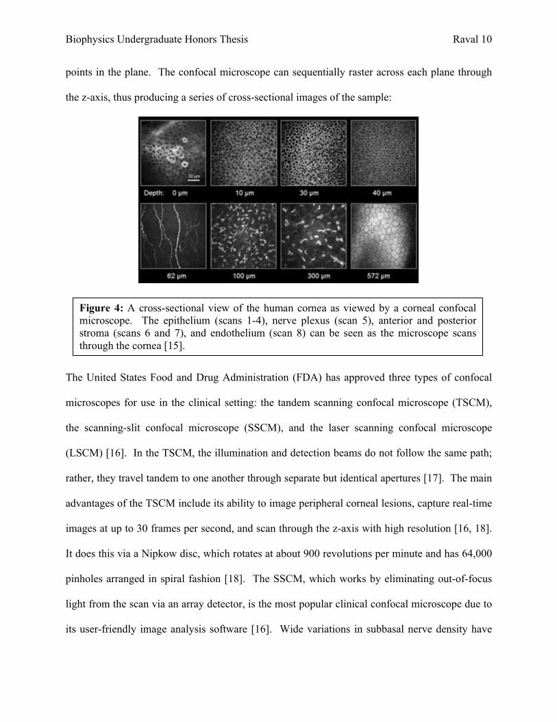
points in the plane. The confocal microscope can sequentially raster across each plane through
the z-axis, thus producing a series of cross-sectional images of the sample:
The United States Food and Drug Administration (FDA) has approved three types of confocal
microscopes for use in the clinical setting: the tandem scanning confocal microscope (TSCM),
the scanning-slit confocal microscope (SSCM), and the laser scanning confocal microscope
(LSCM) [16]. In the TSCM, the illumination and detection beams do not follow the same path;
rather, they travel tandem to one another through separate but identical apertures [17]. The main
advantages of the TSCM include its ability to image peripheral corneal lesions, capture real-time
images at up to 30 frames per second, and scan through the z-axis with high resolution [16, 18].
It does this via a Nipkow disc, which rotates at about 900 revolutions per minute and has 64,000
pinholes arranged in spiral fashion [18]. The SSCM, which works by eliminating out-of-focus
light from the scan via an array detector, is the most popular clinical confocal microscope due to
its user-friendly image analysis software [16]. Wide variations in subbasal nerve density have
Figure 4: A cross-sectional view of the human cornea as viewed by a corneal confocal microscope. The epithelium (scans 1-4), nerve plexus (scan 5), anterior and posterior stroma (scans 6 and 7), and endothelium (scan 8) can be seen as the microscope scans through the cornea [15].

Biophysics Undergraduate Honors Thesis Raval 11
been reported by several studies depending on the type of confocal microscope used. The TSCM
and the SSCM have measured nerve densities of healthy patients in the range from 5.5 µm/mm2
to 11.1 µm/mm2, while the LSCM has measured densities up to 21.7 µm/mm2 [6]. The reason
for these discrepancies lies in the differences in field brightness and image contrast amongst
microscopes; the LSCM and SSCM tend to have greater brightness and contrast than the TSCM
[6]. In addition, due to the high-resolution capabilities of the LSCM, it is able to detect smaller-
caliber nerves, which is why its density estimates can be up to twice those of the SSCM [6].
Clear nerve detection is more difficult at the edges of images due to a decrease in field brightness
[6], but error can be minimized if measurements are made in consistent fashion and the regions
of interest for each image have the same areas.
The most recent confocal microscope and the one that has been used for this study is the LSCM
(Heidelberg Retina Tomograph II Rostock Corneal Module, HRTII) [4]. The main advantage of
using the HRTII over more traditional microscopes like the Confoscan series is that it is able to
produce a series of extremely high-resolution, thin-layer images of the cornea. HRTII generates
high-contrast images at a wavelength of 670nm [6, 15]. Figure 5 below shows how a beam of
laser light is directed through an initial aperture and a partial mirror, passes through a lens, and is
directed through the focal plane of the lens onto a small section of the patient’s cornea. This
light is then reflected off the cornea and travels back through the lens and through the partial
mirror. Another aperture with a small pinhole is placed adjacent to the mirror such that only the
light that is coplanar with the focal plane of the lens is able to pass through to the detector. This
is specifically what makes confocal microscopy unique; the additional pinhole placed within the
focal plane before the detector eliminates any out-of-plane light rays from flooding the detector.

Biophysics Undergraduate Honors Thesis Raval 12
Figure 5: Basic layout of corneal confocal microscopy [6]. Left: the light rays at the focal point of the lens reflect off the cornea and are transmitted through the conjugate aperture to the detector. Right: the light rays that are not reflected off the object plane (dotted lines) are not transmitted through the conjugate aperture to the detector.
The left side of Figure 5 shows how light that is reflected at the focal point of the objective lens
is “co-focused” and confocal to the detector. The right side of Figure 5 depicts the light rays that
are out of the plane of the focal point of the objective lens (slightly anterior or posterior to the
focal point) as solid lines that are defocused at the detector [6]. In other words, these rays are not
coplanar to the lens and so the light rays reflected off this plane will not be transmitted through
the pinhole to the detector. The lens can therefore be adjusted such that the cornea of the patient
is located precisely at its focal point. The brightness of confocal images is dependent on several
factors, such as the intensity of the laser, the radius of the confocal aperture, and the light scatter
and specular reflectivity [6]. Small particles in the epithelial and stromal layers contribute to
light scatter, while sudden changes in refractive index, which occur at the boundaries of the
epithelial and endothelial layers, contribute to specular reflection [6].
Statistical analysis of the data obtained from NeuronJ and CCMetrics will consist of a One-Way
Analysis of Variance (ANOVA), Tukey’s post-hoc test, and the Pearson Coefficient of

Biophysics Undergraduate Honors Thesis Raval 13
Determination. The first two tools, ANOVA and Tukey’s post-hoc test, will be used on the data
obtained from the first part of this study, where the corneal nerve parameters of mean nerve
count, total nerve length, tortuosity, and percentage of primary nerve character, are compared
across patient groups. The third tool, the Pearson Coefficient of Determination (R2 value), will
be used during the multivariable portion of this study, where tortuosity is plotted against mean
nerve count, total nerve length, and percentage of primary nerve character for each patient group.
When comparing two samples, the t-test can be successfully utilized between the groups.
However, the problem with using the t-test when more than two groups are involved, as is the
case in this study, is that false positives tend to arise more often, and an error of 1 – (0.95)n
results, where n is the number of separate t-tests being conducted. One-way ANOVA corrects
this error by comparing all three means simultaneously instead of pair-wise, thereby eliminating
the added type I error probability that arises from performing multiple t-tests. ANOVA works by
generating an F statistic, or F value, which is defined as the variance between sample means
divided by the combined variance within each sample as shown in Equation 1 below [20]. The
p-value can be determined directly from the result of the F test via a correspondence table; the
program Windows OriginLab, automatically converts this F value to its corresponding p-value.
F = MSbg / MSwg
The null hypothesis of the F test is that the means of the samples are all equal. If the p-value that
Equation 1: The F statistic as calculated by one-way ANOVA is defined as the ratio between the “mean square between groups” and the “mean square within groups.” Mean square simply signifies the sum of the squares of the values between or within groups divided by the number of degrees of freedom between or within groups [20].

Biophysics Undergraduate Honors Thesis Raval 14
results from the ANOVA test is greater than 0.05, this indicates that none of the mean values of
the groups are significantly different than the others. However, if the p-value is less than 0.05,
this signifies that one or more of the groups has a significantly different mean value than the
others. Since an ANOVA p-value less than 0.05 does not identify which specific groups are
significantly different from one another, Tukey’s test, one of several post-hoc tests, can be used
to compare the groups pairwise (severe neuropathy and mild or no neuropathy groups, severe
neuropathy and healthy control groups, and mild or no neuropathy and healthy control groups)
without inducing any Type I error. Tukey’s test works based on a value called the Honest
Significant Difference, or HSD [20]. First the test calculates a studentized range statistic (Q),
which is defined as follows:
Q =
ML—MS
sqrt[MSwg / Np/s]
For the 0.05 level of significance, which is used in this study, Windows OriginLab generates
critical values of Q, or values of the statistic that required for significance. The HSD test in turn
uses these critical values to determine the magnitude of the difference between the means of the
two samples needed to be considered “significant” [20]. In other words, Equation 2 above is
rearranged to solve for the difference between ML and MS for the 0.05 level.
Equation 2: Studentized range statistic as calculated by Tukey’s post-hoc HSD test [20]. ML and MS are the larger and smaller means for each pairwise comparison, MSwg is the combined variance within each sample as calculated by ANOVA, and Np/s is the number of values per sample. If these values are not all equal, the harmonic mean of the sample sizes can be determined instead [20].

Biophysics Undergraduate Honors Thesis Raval 15
The last tool used in the statistical analysis portion of this study, the Pearson Coefficient of
Determination, or R2 value, gives a measure of the strength of the correlation between variables.
In other words, the R2 value is the percent of the variation in the y-value that can be explained by
the variation in the x-value [21]. As a general method of determining the qualitative strength of
the correlation from the coefficient value, the following protocol is used [21]:
R value range R2 Value Range Qualitative Strength of Correlation
> 0.90 > 0.81 Very Strong 0.68 – 0.90 0.46 – 0.81 Strong 0.36 – 0.67 0.13 – 0.45 Moderate
< 0.36 < 0.13 Weak
Table 1: Qualitative strength of correlation as determined by the value of Pearson’s Coefficient of Determination [21]. This system will be used to describe the correlations in this study.

Biophysics Undergraduate Honors Thesis Raval 16
Materials/Methods
The confocal data of 31 patients in a prospective clinical study at the Kellogg Eye Center in Ann
Arbor, MI were included in this analysis. The patient sample consisted of three groups: those
with diabetes and proven severe neuropathy (n = 7), those with diabetes and mild or no clinical
evidence of neuropathy (n = 15), and an age-matched healthy control group (n = 9). The
Heidelberg Retina Tomograph (HRT) was used to acquire confocal images of all the corneal
layers in each patient. Five representative scans of the subbasal nerve plexus from the central
cornea were extracted for analysis for each patient. These scans were analyzed using NeuronJ, a
nerve-tracing plugin of the image-processing program ImageJ, as depicted in Figure 6 on the
next page. Image analysis included determining the mean number and length of nerves as well
as giving a breakdown of the type and percentage of nerves – primary, secondary, or tertiary
nerves – in the region analyzed for each patient. A second image analysis program specific to
the assessment of corneal nerves of the subbasal nerve plexus, CCMetrics, was used to collect
the tortuosity data for each patient. CCMetrics contains a built-in algorithm that accumulates the
nerve tortuosity values as each successive nerve is traced within a scan. The greater this
tortuosity value, the greater mean nerve curvature exists in a given scan.

Biophysics Undergraduate Honors Thesis Raval 17
The means and standard deviations of the nerve counts, nerve lengths, and tortuosity values
across the three patient groups were collected and graphed. Statistical analysis was performed
with Windows OriginLab and Microsoft Excel. ANOVA tests in Windows OriginLab were first
used to compare the differences in mean nerve count, total nerve length, and nerve tortuosity
among the three groups of patients. If the null hypothesis of the F test was rejected (p < 0.05),
Tukey’s post-hoc test was used to determine statistically significant differences between groups
in pairwise fashion. The relationships between tortuosity and other parameters studied for these
patients (mean nerve count, total nerve length, and percent primary nerve character) were plotted
for the three groups to determine how these correlations varied based on severity of neuropathy.
Figure 6: NeuronJ Tracing Software (ImageJ Plugin). The subbasal nerve plexus region shown above, captured by the HRT confocal microscope, has an area of 0.16mm2. The red lines signify primary nerves, the blue lines secondary nerves, and the yellow lines tertiary nerves. The white specks are corneal dendrites and were not assessed in this experiment.

Biophysics Undergraduate Honors Thesis Raval 18
To calculate the strength of each correlation, the Pearson Coefficient of Determination, or R2
value, was determined for each regression plot, and the LINEST function in Microsoft Excel was
used to give an estimate of the error in the slope and y-value.

Biophysics Undergraduate Honors Thesis Raval 19
Figure 7: Mean nerve count amongst patient groups. Tukey’s post-hoc test shows that there is a statistically significant difference between the mean nerve count of the severe neuropathy patients (n=9.2) and that of the healthy control group (n=15.2). The error bars represent a single standard deviation.
Results/Discussion
The first objective of this study was to determine how the measured corneal nerve parameters of
mean nerve count, total nerve length, and nerve character varied by level of systemic neuropathy.
The one-way ANOVA test was conducted using the Windows Program Origin; if, and only if, a
p-value less than 0.05 was returned, the Tukey post-hoc test was used to determine the pairs of
groups that were significantly different from one another. These results are shown below.
Degrees of Freedom
Sum of Squares Mean Square F value P value
Model 2 148.374 74.187 3.668 0.038 Error 28 566.300 20.225 - - Total 30 714.674 - - -
0
2
4
6
8
10
12
14
16
18
Severe Neuropathy Mild/No Neuropathy Healthy Controls
Ner
ve C
ount
Patient Group
p < 0.05
p > 0.05 p > 0.05
Table 2: ANOVA test for mean nerve counts amongst patient groups shows that at least one of the groups has a significantly different mean nerve count than the others (p < 0.05).
Biophysics Undergraduate Honors Thesis Raval 20
Figure 8: Total nerve length amongst patient groups. The ANOVA test shows that none of the groups have significantly different total nerve lengths than the other groups, which means that pairwise p values are all greater than 0.05. The error bars represent a single standard deviation.
Healthy Controls Mild/No Neuropathy Severe Neuropathy Healthy Controls - p > 0.05 p < 0.05
Mild/No Neuropathy - - p > 0.05 Severe Neuropathy - - -
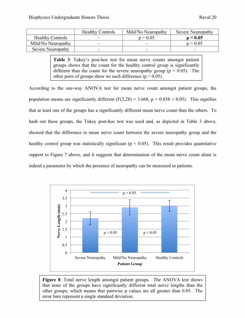
According to the one-way ANOVA test for mean nerve count amongst patient groups, the
population means are significantly different (F(2,28) = 3.668, p = 0.038 < 0.05). This signifies
that at least one of the groups has a significantly different mean nerve count than the others. To
hash out these groups, the Tukey post-hoc test was used and, as depicted in Table 3 above,
showed that the difference in mean nerve count between the severe neuropathy group and the
healthy control group was statistically significant (p < 0.05). This result provides quantitative
support to Figure 7 above, and it suggests that determination of the mean nerve count alone is
indeed a parameter by which the presence of neuropathy can be measured in patients.
0
0.5
1
1.5
2
2.5
3
3.5
4
Severe Neuropathy Mild/No Neuropathy Healthy Controls
Ner
ve L
engt
h (m
m)
Patient Group
p > 0.05
p > 0.05 p > 0.05
Table 3: Tukey’s post-hoc test for mean nerve counts amongst patient groups shows that the count for the healthy control group is significantly different than the count for the severe neuropathy group (p < 0.05). The other pairs of groups show no such difference (p > 0.05).

Biophysics Undergraduate Honors Thesis Raval 21
Table 4: ANOVA test for total nerve lengths amongst patient groups shows that p > 0.05, which means there is no statistically significant difference amongst the patient group. Tukey’s post-hoc test need not be carried out.
Figure 9: Tortuosity values amongst patient groups. The ANOVA test shows that none of the groups have significantly different total nerve lengths than the other groups, which means that pairwise p values are all greater than 0.05. The error bars represent a single standard deviation.
According to the one-way ANOVA test for total nerve lengths amongst patient groups, the
population means are not significantly different (F(2,28) = 1.957, p = 0.160 > 0.05). This
provides quantitative support to Figure 8 above, and it suggests that determination of the total
nerve length alone is not, in itself, a parameter by which the presence of neuropathy can be
measured in patients.
0
5
10
15
20
25
30
35
40
45
Severe Neuropathy Mild/No Neuropathy Healthy Controls
Tort
uosi
ty C
oeffi
cien
t
Patient Group
p > 0.05
p > 0.05 p > 0.05
Degrees of Freedom
Sum of Squares Mean Square F value P value
Model 2 3.004 1.502 1.957 0.160 Error 28 21.488 0.767 - - Total 30 24.492 - - -
Biophysics Undergraduate Honors Thesis Raval 22
Table 5: ANOVA test for tortuosity values amongst patient groups shows that p > 0.05, which means there is no statistically significant difference amongst the patient group. Tukey’s post-hoc test need not be carried out.
According to the one-way ANOVA test for tortuosity values amongst patient groups, the
population means are not significantly different (F(2,28) = 0.65, p = 0.53 > 0.05). This provides
quantitative support to Figure 9 above, and it suggests that determination of the tortuosity
variable alone is not, in itself, a parameter by which the presence of neuropathy can be measured.
The following three figures are pie charts giving a breakdown of the nerve character (primary,
secondary, or tertiary) within each patient group.
4.9, 55%
3.93, 44%
0.05, 1%
Primary
Secondary
Tertiary
Degrees of Freedom
Sum of Squares Mean Square F value P value
Model 2 43.339 21.670 0.650 0.530 Error 28 933.280 33.331 - - Total 30 976.619 - - -
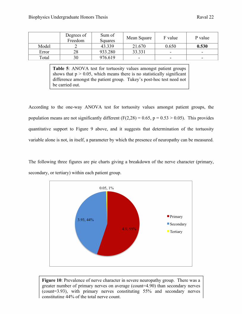
Figure 10: Prevalence of nerve character in severe neuropathy group. There was a greater number of primary nerves on average (count=4.90) than secondary nerves (count=3.93), with primary nerves constituting 55% and secondary nerves constituting 44% of the total nerve count.

Biophysics Undergraduate Honors Thesis Raval 23
Figure 12: Prevalence of nerve character in the healthy control group. The mean number of primary nerves (count=7.28) was less than the number of secondary nerves (count=7.80), with the primary nerves comprising 46% of the total nerve count and the secondary nerves comprising 50% of the total count. The healthy patients exhibited more branched nerves on average than either of the diabetic groups.
6.61, 49%
6.69, 49%
0.23, 2%
Primary
Secondary
Tertiary
7.28, 46%
7.8, 50%
0.68, 4%
Primary
Secondary
Tertiary
Figure 11: Prevalence of nerve character in mild/no neuropathy group. There was an approximately equal number of primary nerves (count=6.61) and secondary nerves (count=6.69), each sharing about 49% of the total nerves in this group of patients.

Biophysics Undergraduate Honors Thesis Raval 24
Within the group of diabetes patients with proven, severe neuropathy, there were a greater
number of primary nerves on average (count=4.90) than secondary nerves (count=3.93), with
primary nerves constituting 55% and secondary nerves constituting 44% of the total nerve count.
Tertiary nerves only contributed to approximately 1% of the total nerve count, with a mean
number of 0.05 nerves. Within the group of diabetes patients with mild or no neuropathy, the
number of primary nerves (count=6.61) and secondary nerves (count=6.69) were approximately
equal, each sharing about 49% of the total nerves in this group of patients. Tertiary nerves only
contributed 2% of the total nerve count, with a mean number of 0.23 nerves. Interestingly,
within the healthy control group, the mean number of primary nerves (count=7.28) was actually
less than the number of secondary nerves (count=7.80), with the primary nerves comprising 46%
of the total nerve count and the secondary nerves comprising 50% of the total count. Tertiary
nerves constituted 4% of the total nerve count, with a mean number of 0.68 nerves. Clearly, the
healthy patients exhibited more branched nerves on average than either of the diabetic groups.
One possible explanation for the fact that there are a higher percentage of secondary nerves than
primary nerves in the healthy control group and a lower percentage of secondary nerves than
primary nerves in the severe neuropathy group is that the corneal nerves of healthy patients can
cross-communicate more effectively. Secondary nerves, which branch directly off primary
nerves and frequently bridge between pairs of nerves, are responsible for spreading action
potentials that come from the trigeminal nerve across the entire subbasal nerve plexus. In
patients with severe diabetic peripheral neuropathy, these secondary nerves are damaged via the
pathophysiological mechanism of the disease, thereby disrupting this efficient communication
method. This explanation is merely a hypothesis, however, and is by no means definitive.

Biophysics Undergraduate Honors Thesis Raval 25
Figure 13: Mean nerve count vs. tortuosity in the healthy control group. The Pearson value shows that there is a very strong, positive correlation between these two variables. There is a slight positive correlation between tortuosity and nerve count, perhaps suggesting that greater nerve curvature allows for a more efficient packing of nerves within a given region of interest. This relationship, however, is not necessarily causal.
The second objective of this study was to determine whether correlations exist between nerve
tortuosity and other parameters, such as mean nerve count, total nerve length, and percent
primary nerve character among the three different groups. This part of the study has the
potential to provide insight into the multivariable effects of diabetic neuropathy, namely, how the
tortuosity value (deemed “tortuosity coefficient” by CCMetric) correlates with each of the nerve
parameters. As tortuosity is an aspect of nerve character that has been studied very little in the
past, analyzing its relationship with nerve parameters can be used to explain nerve behavior in
the subbasal nerve plexus. The following plots depict the relationships between tortuosity and
these nerve parameters. Vertical and horizontal error bars are given as the standard errors of the
means of the nerve count and tortuosity values, respectively.
R² = 0.76838
0
5
10
15
20
25
20 25 30 35 40 45 50
Mea
n N
erve
Cou
nt
Tortuosity Coefficient

Biophysics Undergraduate Honors Thesis Raval 26
Table 6: LINEST Function for Figure 13. The standard deviations of the slope and Y-values are measurements of error within the regression plot.
Figure 13 shows that for the healthy patient group, tortuosity is directly proportional to mean
nerve count. There tends to be greater variability in the mean nerve count at lower tortuosity
values than at higher tortuosity values as can be seen by the larger residuals for the first two
points. The R2 correlation value of 0.768 signifies that there is a 76.8% chance that the data
points are actual solutions to the line of the best fit. The LINEST function in Microsoft Excel
can be used to determine the numerical value of the standard deviation of the y-values.
The relationship between tortuosity and mean nerve count for the severe neuropathy group
shows a much different correlation. Worth noting is the unique, negative fourth-order
polynomial shape of Figure 14 below. Although it could be coincidence that this plot has this
specific shape, especially given the small number of patients in the study group, it is important to
note that the extreme values of tortuosity correlate with the lowest values of nerve count, with
intermediate tortuosity values yielding greater nerve counts. One must be careful not to draw a
large number of conclusions from such a small sample of patients, and further studies should be
carried out using a larger sample size to verify this finding.
LINEST Information Value
Slope 0.309834804
Standard Deviation of Slope 0.135314952
Standard Deviation of Y-Values 2.926879049

Biophysics Undergraduate Honors Thesis Raval 27
Figure 14: Tortuosity vs. mean nerve count in the severe neuropathy group. Although the negative, fourth-order polynomial shape of the best-fit curve may be coincidence, it is worth noting that the highest and lowest values of tortuosity correspond with the lowest mean nerve counts.
Although the correlations depicted above between mean nerve count and nerve tortuosity do not
necessarily signify causation, there are still possible explanations that exist for why the
relationship in the healthy group is positive and why the relationship in the severe neuropathy
group is not. One possible line of reasoning for these correlations is that perhaps neuropathy
causes a lack of communication or signaling between the nerves, so that even if there are a
greater number of nerves within the subbasal nerve plexus of individuals with severe neuropathy,
these nerves are not able to successfully communicate with one another and thus fail to
accommodate for the increased nerve density by increasing their curvature, or tortuosity.
Healthy individuals retain this ability for nerves to cross-communicate and therefore as mean
nerve count increases, the tortuosity also increases, as nerves are able to effectively “sense” their
R² = 0.92562
0
2
4
6
8
10
12
14
16
28 30 32 34 36 38 40 42 44 46
Mea
n N
erve
Cou
nt
Tortuosity Coefficient

Biophysics Undergraduate Honors Thesis Raval 28
Figure 15: Tortuosity vs. total nerve length in the healthy group. The Pearson value shows that there is a strong, positive correlation between these two variables, once again suggesting (but in no way proving) that greater nerve curvature could lead to a higher abundance of nerves within a region.
surroundings and accommodate by becoming more compact. Again, this is by no means a
definitive account of what is actually happening; it is merely speculation by hypothesis and
reasoning.
For the healthy group, it was found that there is a direct correlation between tortuosity and total
nerve length, with greater nerve curvatures showing up in patient scans with greater total nerve
lengths. This finding was similar to that made between tortuosity and mean nerve count.
R² = 0.64133
0 0.5
1 1.5
2 2.5
3 3.5
4 4.5
20 25 30 35 40 45 50
Tota
l Ner
ve L
engt
h (m
m)
Tortuosity Coefficient

Biophysics Undergraduate Honors Thesis Raval 29
Table 7: LINEST Function for Figure 15. The standard deviations of the slope and Y-values are measurements of error within the regression plot.
Figure 16: Tortuosity vs. total nerve length in the severe neuropathy group. Although the negative, fourth-order polynomial shape of the best-fit curve may be coincidence, it is worth noting that the highest and lowest values of tortuosity correspond with the lowest total nerve length.
LINEST Information Value
Slope 0.072585946
Standard Deviation of Slope 0.020516777
Standard Deviation of Y-Values 0.443780407
Severe neuropathy patients with greater tortuosity values also showed a negative, fourth-order
polynomial correlation with total nerve length, similar to the relationship displayed in Figure 14.
R² = 0.87597
0
0.5
1
1.5
2
2.5
3
3.5
4
28 30 32 34 36 38 40 42 44 46
Tota
l Ner
ve L
engt
h (m
m)
Tortuosity Coefficient

Biophysics Undergraduate Honors Thesis Raval 30
Since total nerve length and mean nerve count within a scan are related to nerve density, the
reasoning that the nerves of patients with severe peripheral neuropathy are not able to
communicate as effectively as those of healthy patients and curve more in regions of higher
nerve densities makes intuitive sense.
There is another unique characteristic about the healthy control group that fails to show in either
of the other two groups. With respect to tortuosity coefficient versus percentage of primary
nerves (out of total number of primary, secondary, and tertiary nerves), the healthy control group
shows a moderately-strong negative correlation as depicted in Figure 17, while there is no
correlation present in the other two groups.
R² = 0.27606
0 0.1 0.2 0.3 0.4 0.5 0.6 0.7 0.8 0.9
20 25 30 35 40 45 50
% P
rimar
y N
erve
s
Tortuosity Coefficient
Figure 17: Tortuosity vs. percentage of primary nerves in the healthy group. The Pearson value shows that there is a moderate, negative correlation between these two variables.
Biophysics Undergraduate Honors Thesis Raval 31
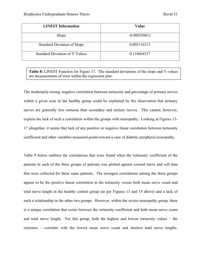
Table 8: LINEST Function for Figure 17. The standard deviations of the slope and Y-values are measurements of error within the regression plot.
LINEST Information Value
Slope -0.008358811
Standard Deviation of Slope 0.005116213
Standard Deviation of Y-Values 0.110664317
The moderately-strong, negative correlation between tortuosity and percentage of primary nerves
within a given scan in the healthy group could be explained by the observation that primary
nerves are generally less tortuous than secondary and tertiary nerves. This cannot, however,
explain the lack of such a correlation within the groups with neuropathy. Looking at Figures 13-
17 altogether, it seems that lack of any positive or negative linear correlation between tortuosity
coefficient and other variables measured points toward a case of diabetic peripheral neuropathy.
Table 9 below outlines the correlations that were found when the tortuosity coefficient of the
patients in each of the three groups of patients was plotted against corneal nerve and cell data
that were collected for these same patients. The strongest correlations among the three groups
appear to be the positive linear correlation in the tortuosity versus both mean nerve count and
total nerve length in the healthy control group (as per Figures 13 and 15 above) and a lack of
such a relationship in the other two groups. However, within the severe neuropathy group, there
is a unique correlation that exists between the tortuosity coefficient and both mean nerve count
and total nerve length. For this group, both the highest and lowest tortuosity values – the
extremes – correlate with the lowest mean nerve count and shortest total nerve lengths.

Biophysics Undergraduate Honors Thesis Raval 32
Although it is not clear whether the values between these extremes approximate a negative
parabola or negative fourth-order polynomial curve, it is evident in Figures 14 and 16 below that
patients with severe diabetic neuropathy show the lowest values of nerve counts and nerve
lengths at extreme tortuosity values.
Severe Neuropathy Mild/No Neuropathy Healthy Controls Correlation Strength Correlation Strength Correlation Strength
Tortuosity vs. Mean Nerve Count
Lowest mean nerve counts at extreme tortuosity
values
R2 = 0.93 (Very
strong) none N/A (+) linear
R2 = 0.77 (Very
strong)
Tortuosity vs. Total Nerve Length
Lowest total nerve lengths
at extreme tortuosity
values
R2 = 0.88 (Very
strong) none N/A (+) linear R2 = 0.64
(Strong)
Tortuosity vs. % Primary Nerve
Character
none N/A none N/A (–) linear R2 = 0.28 (Moderate)
Table 9: Multivariable Corneal Correlations

Biophysics Undergraduate Honors Thesis Raval 33
Conclusions
In-vivo confocal corneal microscopy has proven to be an effective clinical method to assess the
nerves in the subbasal nerve plexus of the cornea. The relationships between tortuosity and
nerve count, nerve length, basal cell density, and percent primary nerve character have shown
that there are correlative differences amongst healthy patients and those expressing forms of
diabetic neuropathy. This study has shown that there is a statistically significant difference (p <
0.05) in the mean nerve count of corneal nerves between healthy patients and severe neuropathy
patients, proving correct the hypothesis that patients with neuropathy express a lower mean nerve
count. It has also shown that patients who express high tortuosity values along with high nerve
counts and lengths, as depicted by the strong correlations in the multivariable study, are more
likely to be healthy than those who express high tortuosity values with low nerve counts and
lengths. A strong positive, linear correlation between tortuosity versus both mean nerve count
and total nerve length, and a negative linear correlation between tortuosity versus primary nerve
percentage, are not characteristic of patient groups that express some form of diabetic
neuropathy.
This study can be improved in several ways. First, the patient sample size used was not large
enough to elicit trends with great confidence. In future studies, each of the three groups should
have the same number of patients, with at least 20 patients per group. In the current study, the
severe neuropathy group only contained seven subjects, which makes it difficult to claim that the
relationships between tortuosity and other nerve parameters are reliable. Once a large number of
patients are sampled for this study, multivariable regression equations can be developed and used
to determine a patient’s level of neuropathy with a much higher confidence. This project can

Biophysics Undergraduate Honors Thesis Raval 34
also be improved by using an automated MATLAB script to perform rapid, reliable image
analysis of patient scans rather than having to manually trace the nerves of each patient using
NeuronJ and CCMetric. A MATLAB algorithm is currently being developed by a group of
engineering students at the University of Michigan that sequentially runs through the confocal
scans, defines a threshold value for each image, eliminates background noise (dendrites and
microdots that are not needed for nerve analysis), and provides information on nerve parameters,
such as nerve count and length, for each scan. Automating this process will speed up data
analysis tremendously and allow for the confocal scans of large numbers of patients to be
analyzed with greater precision. In future projects, the specificity and sensitivity of this updated
model will be tested so that it can be used in the clinical setting as a valid diagnostic for diabetic
neuropathy.

Biophysics Undergraduate Honors Thesis Raval 35
Acknowledgments
A special thanks goes out to Roni Shtein, MD, MS, for her guidance and mentorship of this
project as well as her expertise in the fields of diabetic neuropathy and confocal corneal
microscopy. A sincere thanks goes out to Stephen Lentz, PhD, for allowing use of his lab’s
computers to carry out the digital analysis for this experiment. Thanks to Professor Jennifer
Ogilvie of the University of Michigan Biophysics Department for her authorization of this study,
and to Rayaz Malik, PhD, of the University of Manchester for leading development of
CCMetric, one of the automated nerve tracing programs used for this project. Finally, thanks
goes out to the cornea and diabetes clinics of the Kellogg Eye Center in Ann Arbor, MI, where
all patient data was collected.

Biophysics Undergraduate Honors Thesis Raval 36
References
[1] "Diabetes Statistics." Diabetes.org. American Diabetes Association, 2012. Web. 3 Oct. 2013.
[2] "Facts About The Cornea and Corneal Disease." National Institutes of Health. National Eye
Institute, May 2013. Web. 3 Oct. 2013.
[3] Lagali, Neil, Johan Germundsson, and Per Fagerholm. "The Role of Bowman’s Layer in
Corneal Regeneration after Phototherapeutic Keratectomy: A Prospective Study Using In Vivo
Confocal Microscopy." Investigative Ophthalmology & Visual Science 50.9 (2009): 4192-198. 5
Oct. 2013.
[4] Tavakoli, Mitra, Parwez Hossain, and Rayaz A. Malik. "Clinical Applications of Corneal
Confocal Microscopy." Journal of Clinical Ophthalmology 2.2 (2008): 435-45. Print.
[5] Masters, Barry R., and Andreas A. Thaer. "In Vivo Human Corneal Confocal Microscopy of
Identical Fields of Subepithelial Nerve Plexus, Basal Epithelial, and Wing Cells at Different
times." Microscopy Research and Technique 29.5 (2005): 350-56. Wiley Online Library. Web. 2
Oct. 2013.
[6] Erie, Jay C., Jay W. McLaren, and Sanjay V. Patel. "Confocal Microscopy in
Ophthalmology." American Journal of Ophthalmology 148.5 (2009): 639-46. Web. 2 Oct. 2013.
[7] Al-Aqaba, Mouhamed A., Usama Fares, Hanif Suleman, James Lowe, and Harminder S.
Dua. "Architecture and Distribution of Human Corneal Nerves." British Journal of
Ophthalmology 94.6 (2010): 784-89. Web.
[8] Wells, Jill R., MD, and Marc A. Michelson, MD. "Diagnosing and Treating Neurotrophic
Keratopathy." EyeNet Magazine 2013. Web. 2 Oct. 2013.

Biophysics Undergraduate Honors Thesis Raval 37
[9] Chiou, Auguste G.Y., MD, Stephen C. Kaufman, MD, PhD, Herbert E. Kaufman, MD, and
Roger W. Beuerman, PhD. "Clinical Corneal Confocal Microscopy." Survey of Ophthalmology
51.5 (2006): 482-500. Print.
[10] Oliveira-Soto, L., and N. Efron. "Morphology of Corneal Nerves Using Confocal
Microscopy." Cornea 20.4 (2001): 374-84. PubMed. US National Library of Medicine. Web. 2
Oct. 2013.
[11] "Diabetic Neuropathy." Mayo Clinic. Mayo Foundation for Medical Education and
Research, 06 Mar. 2012. Web. 4 Oct. 2013.
[12] "Diabetic Neuropathies: The Nerve Damage of Diabetes." National Diabetes Information
Clearinghouse (NDIC). National Institutes of Health, 25 June 2012. Web. 16 Dec. 2013.
[13] Efron, N. "Ophthalmic Markers of Diabetic Neuropathy." Optometry & Visual Science 88.6
(2011): 661-83. PubMed. National Institutes of Health. Web. 4 Oct. 2013.
[14] Jalbert, I., F. Stapleton, and M. Coroneo. "In Vivo Confocal Microscopy of the Human
Cornea." British Journal of Ophthalmology 87.2 (2003): 225-36. National Institutes of Health.
Web. 7 Oct. 2013.
[15] "HRT Rostock Cornea Module." Heidelberg Engineering. Heidelberg Engineering GmbH,
2013. Web. 7 Oct. 2013.
[16] "Confocal Microscopy." The Ophthalmic News & Education Network. American Academy
of Ophthalmology, 2013. Web. 7 Oct. 2013.
[17] Spring, Kenneth R., Thomas J. Fellers, and Michael W. Davidson. "Confocal Microscope
Scanning Systems." FluoView Resource Center. Olympus Corporation, 2009. Web. 7 Oct. 2013.

Biophysics Undergraduate Honors Thesis Raval 38
[18] Dhaliwal, Jasmeet S., Stephen C. Kaufman, and Auguste GY Chiou. "Current Applications
of Clinical Confocal Microscopy." Current Opinion in Ophthalmology 18.4 (2007): 300-07.
Print.
[19] Patel, Dipika V., and Charles N.J. McGhee. "Contemporary in Vivo Confocal Microscopy
of the Living Human Cornea Using White Light and Laser Scanning Techniques: A Major
Review." Clinical & Experimental Ophthalmology 35.1 (2007): 71-88. Print.
[20] Lowry, Richard. Concepts and Applications of Inferential Statistics. Vassar Stats, 2013.
Web. 9 Oct. 2013.
[21] Taylor, Richard, EDD, RDCS. "Interpretation of the Correlation Coefficient." Journal of
Diagnostic Medical Sonography 6.1 (1990): 35-39. Web. 13 Oct. 2013.