in copyright - non-commercial use permitted rights ...26212/... · a geometric framework for visual...
TRANSCRIPT

Research Collection
Doctoral Thesis
A geometric framework for visual grouping
Author(s): Turina, Andreas
Publication Date: 2003
Permanent Link: https://doi.org/10.3929/ethz-a-004488586
Rights / License: In Copyright - Non-Commercial Use Permitted
This page was generated automatically upon download from the ETH Zurich Research Collection. For moreinformation please consult the Terms of use.
ETH Library

DISS. ETH NO. 14919
A Geometric Framework for Visual Grouping
A dissertation submitted to the
SWISS FEDERAL INSTITUTE OF TECHNOLOGY ZURICH
for the degree ofDoctor of Technical Sciences
presented by
ANDREAS TURINA
Dipl. El.-Ing. ETH
born 4th of June, 1971citizen of
Fallanden, Switzerland
accepted on the recommendation of
Prof. Dr. Luc Van Gool, examinerProf. Dr. Bernt Schiele, co-examiner
2002


To My Parents


Abstract
This dissertation deals with a geometric framework for the efficient detection of
regular repetitions of planar (but not necessarily coplanar) patterns. Such pattern
repetitions are ubiquitous: Tilings of a floor, repetitions of windows on a building
facade, mirror-symmetries etc. Basically, two aspects are of importance: There is a
repeating pattern, and the repetition is carried out in a regular manner.
The desire for an automatic detection of such groupings is an old challenge in Com-
puter Vision, and an immense number of contributions exists, most of them address-
ing the grouping of low-level features, like edges and contours, assuming pseudo-
orthographic projection models. Geometric grouping contributions that deal with
full perspective skew are comparatively new.
Most of these earlier approaches are characterized by their extensive use of combina-
torial techniques, which renders the grouping process fairly inefficient. In addition,
they focus on one particular grouping type only, restricted to a narrow range of
features, often specified by the user beforehand.
The grouping system proposed in this dissertation avoids the shortcomings of earlier
contributions. The novelty of our approach is that it is efficient by banning exten-
sive combinatorics from all stages. Furthermore, our approach is more general in
that all groupings related by planar homologies are detected. These include period-
icities, mirror-symmetries and point-symmetries that have traditionally been dealt
with separately. The approach can handle perspective distortions. It avoids to get
trapped in combinatorics through invariant-based hashing for pattern matching and
through Hough transforms for the detection of fixed structures.
At the heart of our system lie the fixed structures of the transformations that de-
scribe these regular configurations. Fixed structures are geometric entities, like
points and lines, that remain fixed under both the original symmetry operation in
the scene and the transformation that relates repeating patterns in the image. The
knowledge of fixed structures drastically reduces the complexity (degrees of freedom)
of the problem, and therefore the main effort is their efficient extraction.
A first step detects small, repeating planar patches near points of interest in the
image using affinely invariant neighbourhoods. The way how they are extracted
i

ii
makes them immune to affine geometric transformations and linear photometric
changes. Invariant neighbourhoods are characterized by a feature vector of moment
invariants that implicitly describe the underlying intensity profile in an invariant
way again. Pattern repetitions then translate to clusters in this feature space, and
similar patterns can be found efficiently using invariant-based indexing.
In a second step, clusters of similar invariant neighbourhoods are analyzed for their
regularity using a cascaded version of the Hough transform. The end products are
candidates for fixed structures, found in a non-combinatorial way. A single point /
neighbourhood match then suffices to lift the remaining degree of freedom in order
to set up a grouping (i.e. planar homology) hypothesis. Finally, hypotheses are
validated for their correctness based on a correlation-based procedure that delineates
the symmetric parts in the image. The system has been applied to a wealth of regular
images to demonstrate its performance.

Kurzfassung
Diese Dissertation behandelt die effiziente Detektion sich regular wiederholender,
planarer (aber nicht notwendigerweise koplanarer) Muster in Bildern. Regulare Re-
petitionen dieser Art sind fast allgegenwartig: man denke z.B. an einen gekachelten
Boden, die regelmassige Anordnung von Fenstern einer Hausfassade, Spiegelsym-
metrien etc. Im wesentlichen gibt es dabei zwei Feststellungen: Es gibt ein sich
wiederholendes Muster, und die Art der Wiederholung vollzieht sich nach strengen
Regeln.
Der Wunsch, solche Gruppierungen automatisch in Bildern zu finden, reicht in der
’Computer Vision’ weit zuruck, und eine grosse Anzahl von Beitragen sind mit der
Zeit entstanden. Die meisten davon handeln uber Gruppierung von Bildprimitiven,
z.B. Kantenpunkte und Konturen, unter Annahme von pseudo-orthographischer
Projektion. Geometrische Ansatze, welche auch perspektivische Verzerrungen be-
handeln, sind vergleichsweise neu.
Ein gewichtiger Nachteil der meisten fruheren Gruppierungsansatze stellt deren star-
ker Einsatz kombinatorischer Methoden dar, was sich sehr ungunstig auf die Effizienz
auswirkt. Zusatzlich sind diese Systeme fur die Detektion eines einzigen Gruppie-
rungstyps massgeschneidert, wobei man sich nur auf ein paar wenige, spezifische
Merkmale abstutzt. Noch dazu mussen diese oft vom Benutzer angegeben werden.
Das in dieser Dissertation vorgeschlagene System behebt viele Defizite fruherer
Ansatze. Umfangreiche kombinatorische Methoden werden hier in allen Bereichen
strikt vermieden. Eine weitere Neuerung stellt die Tatsache dar, dass unser Gruppie-
rungsansatz allgemeiner ist, indem er auf planaren Homologien basiert. Damit wer-
den Periodizitaten, Spiegel- und Punktsymmetrien im gleichen Zug erkannt, und das
unter Einbezug perspektivischer Verzerrungen. Dies wird mittels invarianz-basierten
Hashing Methoden und Hough-Techniken erreicht.
Unserem System liegt das Konzept der sog. fixen Strukturen zugrunde. Dabei han-
delt es sich um Punkte und Geraden, welche unter der originalen Symmetrieoperati-
on im Raum sowie deren Abbildung im Bild erhalten bleiben. Sind diese Strukturen
einmal bekannt, dann reduziert sich die Komplexitat (Anzahl Freiheitsgrade) be-
trachtlich. Das Ziel ist folglich, diese fixen Strukturen auf effiziente Weise zu finden.
iii

iv
In einem ersten Schritt wird nach Wiederholungen kleiner, planarer Segmente ge-
sucht. Dazu kommen affin-invariante Umgebungen zum Einsatz. Die Art und Weise,
wie solche Umgebungen extrahiert werden, macht sie immun gegenuber affinen geo-
metrischen Verzerrungen sowie linearen, photometrischen Anderungen. Jede einzel-
ne solche Umgebung wird durch einen Merkmalsvektor charakterisiert, der wieder-
um aus Momentinvarianten besteht. Dieser Vektor beschreibt das Intensitatsprofil
von affin-invarianten Umgebungen wiederum auf invariante Weise. Die Detektion
sich wiederholender Bildsegmente verlagert sich damit auf die Identifikation von
Anhaufungen in diesem Merkmalsraum. Indizierungstechniken tragen dabei zur Ef-
fizienzsteigerung bei.
In einem zweiten Schritt werden gefundene Wiederholungen solcher Bildsegmente
auf deren Regularitat gepruft. Dies wird uber eine spezielle Version der Hough Trans-
formation erreicht, welche als Endprodukt mogliche Kandidaten fur fixe Strukturen
liefert, wiederum auf nicht-kombinatorische Art. Eine einzelne Punktkorrespondenz
genugt nun, um eine Gruppierungshypothese aufzustellen. Ein korrelations-basiertes
Verfahren uberpruft die Hypothese auf ihre Richtigkeit und segmentiert dabei die
Gruppierung im Bild. Die Leistungsfahigkeit des Systems wird anhand einer Vielzahl
unterschiedlicher Bilder demonstriert.
Acknowledgement
First, I would like to thank my supervisor, Prof. Dr. Luc Van Gool, for both
his lead and his valuable support during the entire duration of my dissertation.
Apart from his brilliant professional skills, I highly appreciated his willingness to
provide me with everything that I needed for the daily work. I also appreciated his
offers to travel to remote locations for meetings and conferences around the globe;
a necessity for establishing contacts with the Computer Vision community. I also
thank Prof. Dr. Bernt Schiele for his role as co-referee and his advice on various
technical problems.
Special thanks go to Dr. Tinne Tuytelaars whose aid substantially shaped this
dissertation. With her as a designated tutor from the very beginning, I really enjoyed
the privilege of a close collaboration with a skilled and experienced researcher who
followed my work with great interest. Our fruitful exchange of ideas, problems,
solutions, software and data on an almost daily basis was of inestimable value.
I am grateful to all members of the Computer Vision Laboratory at ETH (“BIWI”)
who supported me during the work on my PhD thesis. Furthermore, I am especially
thankful to our system manager Manuel Oetiker, whose technical help and manage-
ment skills of a complex computational infrastructure provided the necessary basics
so essential for the work in Computer Vision.
I especially want to express my thanks to my parents, Marko and Helga Turina,
who made my studies at ETH Zurich possible and who gave me their unconditional
support in all phases of my life.
Andreas Turina
v


Contents
Abstract i
Kurzfassung iii
Contents xi
List of Figures xiv
List of Tables xv
1 Introduction 1
1.1 Rationale . . . . . . . . . . . . . . . . . . . . . . . . . . . . . . . . . 2
1.2 Possible Applications . . . . . . . . . . . . . . . . . . . . . . . . . . . 3
1.3 Main Contributions . . . . . . . . . . . . . . . . . . . . . . . . . . . . 4
1.4 Strategy and System Overview . . . . . . . . . . . . . . . . . . . . . . 4
1.4.1 Regular Repetitions . . . . . . . . . . . . . . . . . . . . . . . . 5
1.4.2 The Danger of Resorting to Combinatorics . . . . . . . . . . . 5
1.4.3 Efficient Detection of Repetitions . . . . . . . . . . . . . . . . 7
1.4.4 Efficient Detection of Regularities . . . . . . . . . . . . . . . . 8
1.5 Outline of the Thesis . . . . . . . . . . . . . . . . . . . . . . . . . . . 9
2 Tour d’horizon: From the Early Days to State of the Art 11
2.1 Gestalt Laws . . . . . . . . . . . . . . . . . . . . . . . . . . . . . . . 12
2.2 Grouping Based on Gestalt Laws . . . . . . . . . . . . . . . . . . . . 12
vii

viii Contents
2.3 Grouping Based on Geometry . . . . . . . . . . . . . . . . . . . . . . 14
2.3.1 The Affine Case . . . . . . . . . . . . . . . . . . . . . . . . . . 15
2.3.2 The Perspective Case . . . . . . . . . . . . . . . . . . . . . . . 17
2.4 Analysis . . . . . . . . . . . . . . . . . . . . . . . . . . . . . . . . . . 20
2.4.1 Generality . . . . . . . . . . . . . . . . . . . . . . . . . . . . . 20
2.4.2 Features . . . . . . . . . . . . . . . . . . . . . . . . . . . . . . 22
2.4.3 Efficiency . . . . . . . . . . . . . . . . . . . . . . . . . . . . . 23
2.5 Summary and Conclusions . . . . . . . . . . . . . . . . . . . . . . . . 25
3 Fixed Structures - Key to Efficiency 27
3.1 Plane Projective Transformations . . . . . . . . . . . . . . . . . . . . 28
3.1.1 Coarse Structure . . . . . . . . . . . . . . . . . . . . . . . . . 28
3.2 Fixed Structures and Subgroups . . . . . . . . . . . . . . . . . . . . . 29
3.2.1 Fixed Structures . . . . . . . . . . . . . . . . . . . . . . . . . 29
3.2.2 Subgroups Defined by Fixed Structures . . . . . . . . . . . . . 30
3.3 Fixed Structures for Grouping . . . . . . . . . . . . . . . . . . . . . . 32
3.3.1 Conjugate Symmetry . . . . . . . . . . . . . . . . . . . . . . . 32
3.4 Planar Homologies . . . . . . . . . . . . . . . . . . . . . . . . . . . . 33
3.5 Elations . . . . . . . . . . . . . . . . . . . . . . . . . . . . . . . . . . 35
3.6 Summary and Conclusions . . . . . . . . . . . . . . . . . . . . . . . . 38
4 Basic Technologies I: Affinely Invariant Neighbourhoods 39
4.1 Motivation . . . . . . . . . . . . . . . . . . . . . . . . . . . . . . . . . 39
4.2 Affinely Invariant Neighbourhoods . . . . . . . . . . . . . . . . . . . . 42
4.2.1 Geometry-based Neighbourhoods . . . . . . . . . . . . . . . . 45
4.2.2 Intensity-based Neighbourhood Extraction . . . . . . . . . . . 50
4.3 Neighbourhood Description . . . . . . . . . . . . . . . . . . . . . . . 52
4.4 Conclusion . . . . . . . . . . . . . . . . . . . . . . . . . . . . . . . . . 53

Contents ix
5 Basic Technologies II: The Cascaded Hough Transform 55
5.1 The Hough Transform Revisited . . . . . . . . . . . . . . . . . . . . . 55
5.2 The Cascaded Hough Transform . . . . . . . . . . . . . . . . . . . . . 56
5.2.1 The CHT-point . . . . . . . . . . . . . . . . . . . . . . . . . . 58
5.2.2 Homogeneous Representation of CHT-points . . . . . . . . . . 58
5.3 CHT Arithmetics . . . . . . . . . . . . . . . . . . . . . . . . . . . . . 59
5.3.1 Image Frame −→ CHT Frame . . . . . . . . . . . . . . . . . . 60
5.3.2 CHT-Frame → Image-Frame . . . . . . . . . . . . . . . . . . . 62
5.4 Applying the CHT . . . . . . . . . . . . . . . . . . . . . . . . . . . . 63
5.4.1 Hough Transform . . . . . . . . . . . . . . . . . . . . . . . . . 63
5.4.2 Peak Extraction . . . . . . . . . . . . . . . . . . . . . . . . . . 64
5.4.3 Peak Validation . . . . . . . . . . . . . . . . . . . . . . . . . . 67
5.5 Example . . . . . . . . . . . . . . . . . . . . . . . . . . . . . . . . . . 68
5.6 Discussion . . . . . . . . . . . . . . . . . . . . . . . . . . . . . . . . . 71
5.6.1 Accuracy vs. Resolution . . . . . . . . . . . . . . . . . . . . . 71
5.6.2 Computational Complexity . . . . . . . . . . . . . . . . . . . . 71
5.6.3 Peak Extraction . . . . . . . . . . . . . . . . . . . . . . . . . . 72
5.6.4 Alternative Parameterization . . . . . . . . . . . . . . . . . . 72
5.7 Summary and Conclusion . . . . . . . . . . . . . . . . . . . . . . . . 73
6 Detection of Repetitions 75
6.1 Introduction . . . . . . . . . . . . . . . . . . . . . . . . . . . . . . . . 75
6.2 Invariant Description . . . . . . . . . . . . . . . . . . . . . . . . . . . 76
6.2.1 Generic Affinely Invariant Feature Vectors . . . . . . . . . . . 77
6.2.2 Normalized Feature Vectors . . . . . . . . . . . . . . . . . . . 77
6.3 Neighbourhood Comparison . . . . . . . . . . . . . . . . . . . . . . . 82
6.3.1 Feature Vector Comparison . . . . . . . . . . . . . . . . . . . 83
6.3.2 Correlation-based Comparison of Affinely
Invariant Neighbourhoods . . . . . . . . . . . . . . . . . . . . 85

x Contents
6.3.3 Other Comparison Methods . . . . . . . . . . . . . . . . . . . 85
6.4 Matching / Clustering . . . . . . . . . . . . . . . . . . . . . . . . . . 87
6.5 Example . . . . . . . . . . . . . . . . . . . . . . . . . . . . . . . . . . 89
6.6 Discussion . . . . . . . . . . . . . . . . . . . . . . . . . . . . . . . . . 90
6.7 Summary and Conclusions . . . . . . . . . . . . . . . . . . . . . . . . 92
7 Detection of Regularities 93
7.1 Introduction . . . . . . . . . . . . . . . . . . . . . . . . . . . . . . . . 93
7.2 Finding Fixed Structures . . . . . . . . . . . . . . . . . . . . . . . . . 94
7.2.1 Candidate Pencils of Fixed Lines . . . . . . . . . . . . . . . . 94
7.2.2 Candidate Lines of Fixed Points . . . . . . . . . . . . . . . . . 96
7.2.3 Example . . . . . . . . . . . . . . . . . . . . . . . . . . . . . . 97
7.3 Finding the Groupings . . . . . . . . . . . . . . . . . . . . . . . . . . 101
7.4 Hypotheses Validation . . . . . . . . . . . . . . . . . . . . . . . . . . 101
7.5 Discussion . . . . . . . . . . . . . . . . . . . . . . . . . . . . . . . . . 104
7.5.1 Advantages of the CHT . . . . . . . . . . . . . . . . . . . . . 104
7.5.2 Parameters . . . . . . . . . . . . . . . . . . . . . . . . . . . . 104
7.5.3 Computation Times . . . . . . . . . . . . . . . . . . . . . . . 105
7.5.4 CHT vs. Gaussian Sphere . . . . . . . . . . . . . . . . . . . . 106
7.6 Summary and Conclusions . . . . . . . . . . . . . . . . . . . . . . . . 106
8 Experimental Results 109
8.1 Introduction . . . . . . . . . . . . . . . . . . . . . . . . . . . . . . . . 109
8.2 General Planar Homologies . . . . . . . . . . . . . . . . . . . . . . . . 110
8.3 Elations . . . . . . . . . . . . . . . . . . . . . . . . . . . . . . . . . . 112
8.4 Conclusion . . . . . . . . . . . . . . . . . . . . . . . . . . . . . . . . . 116
9 Conclusion 119
9.1 Summary . . . . . . . . . . . . . . . . . . . . . . . . . . . . . . . . . 119
9.2 Discussion and Outlook . . . . . . . . . . . . . . . . . . . . . . . . . 121
9.2.1 Improvements . . . . . . . . . . . . . . . . . . . . . . . . . . . 121
9.2.2 Future Work . . . . . . . . . . . . . . . . . . . . . . . . . . . . 122

Contents xi
A Linear Discriminant Analysis 125
A.1 Principle . . . . . . . . . . . . . . . . . . . . . . . . . . . . . . . . . . 125
A.2 Covariance Matrix Based on Tracking Experiments . . . . . . . . . . 127
B Image Database Overview 129
Bibliography 131

List of Figures
1.1 A regular repetition of floor tiles, distorted by perspective skew. . . . 6
3.1 Classificatory structure of subgroups for fixed points and lines. . . . . 31
3.2 Distortion of a mirror-symmetry . . . . . . . . . . . . . . . . . . . . . 32
3.3 Planar homology examples . . . . . . . . . . . . . . . . . . . . . . . . 35
3.4 Visualization of group action . . . . . . . . . . . . . . . . . . . . . . . 37
4.1 Effects of perspective skew . . . . . . . . . . . . . . . . . . . . . . . . 40
4.2 Neighbourhood example . . . . . . . . . . . . . . . . . . . . . . . . . 43
4.3 Harris corner points . . . . . . . . . . . . . . . . . . . . . . . . . . . . 45
4.4 Local intensity extrema. . . . . . . . . . . . . . . . . . . . . . . . . . 46
4.5 Neighbourhood construction for curved edges . . . . . . . . . . . . . . 46
4.6 Neighbourhood construction for straight edges . . . . . . . . . . . . . 48
4.7 Neighbourhood construction for homogeneous regions . . . . . . . . . 49
4.8 Example of homogeneous neighbourhoods . . . . . . . . . . . . . . . 50
4.9 Intensity-based neighbourhood construction. . . . . . . . . . . . . . . 51
4.10 Intensity-based neighbourhood example . . . . . . . . . . . . . . . . . 52
5.1 CHT subspaces . . . . . . . . . . . . . . . . . . . . . . . . . . . . . . 57
5.2 Different point representations . . . . . . . . . . . . . . . . . . . . . . 60
5.3 Effect of smoothing . . . . . . . . . . . . . . . . . . . . . . . . . . . . 65
5.4 CHT buffer example . . . . . . . . . . . . . . . . . . . . . . . . . . . 66
5.5 Buffer sampling . . . . . . . . . . . . . . . . . . . . . . . . . . . . . . 67
xii

List of Figures xiii
5.6 CHT example: input . . . . . . . . . . . . . . . . . . . . . . . . . . . 68
5.7 CHT example: buffers . . . . . . . . . . . . . . . . . . . . . . . . . . 69
5.8 CHT example: collinear structures . . . . . . . . . . . . . . . . . . . 70
5.9 CHT example: second Hough . . . . . . . . . . . . . . . . . . . . . . 70
5.10 CHT example: pencils of fixed lines . . . . . . . . . . . . . . . . . . . 71
6.1 Original image and neighbourhoods . . . . . . . . . . . . . . . . . . . 89
6.2 Feature space . . . . . . . . . . . . . . . . . . . . . . . . . . . . . . . 90
6.3 Clusters in the image and feature space . . . . . . . . . . . . . . . . . 91
7.1 Pencil of fixed lines example . . . . . . . . . . . . . . . . . . . . . . . 98
7.2 Fixed structures example . . . . . . . . . . . . . . . . . . . . . . . . . 99
7.3 Lines of fixed points example . . . . . . . . . . . . . . . . . . . . . . 100
7.4 Effect of a global warp . . . . . . . . . . . . . . . . . . . . . . . . . . 102
7.5 Validation result . . . . . . . . . . . . . . . . . . . . . . . . . . . . . 104
8.1 Butterfly example I . . . . . . . . . . . . . . . . . . . . . . . . . . . . 110
8.2 Butterfly example II . . . . . . . . . . . . . . . . . . . . . . . . . . . 111
8.3 Carpet example I . . . . . . . . . . . . . . . . . . . . . . . . . . . . . 111
8.4 Carpet example II . . . . . . . . . . . . . . . . . . . . . . . . . . . . 111
8.5 Books example I . . . . . . . . . . . . . . . . . . . . . . . . . . . . . 112
8.6 Book example II . . . . . . . . . . . . . . . . . . . . . . . . . . . . . 113
8.7 Beer-box example I . . . . . . . . . . . . . . . . . . . . . . . . . . . . 113
8.8 Beer-box example II . . . . . . . . . . . . . . . . . . . . . . . . . . . 114
8.9 Building facade example I . . . . . . . . . . . . . . . . . . . . . . . . 114
8.10 Building facade example II . . . . . . . . . . . . . . . . . . . . . . . . 115
8.11 Visualization of the symmetry density. . . . . . . . . . . . . . . . . . 115
8.12 Router example . . . . . . . . . . . . . . . . . . . . . . . . . . . . . . 116
A.1 Initial cluster configuration. . . . . . . . . . . . . . . . . . . . . . . . 126
A.2 Transformed dataset after rotation and scaling. . . . . . . . . . . . . 126

xiv List of Figures
A.3 Situation after the second transform. . . . . . . . . . . . . . . . . . . 127
B.1 Example images the system was applied to. . . . . . . . . . . . . . . . 129
B.2 Example images the system was applied to (ctd.) . . . . . . . . . . . 130

List of Tables
2.1 Classificatory structure . . . . . . . . . . . . . . . . . . . . . . . . . . 12
3.1 Hierarchy of subgroups . . . . . . . . . . . . . . . . . . . . . . . . . . 29
6.1 Moment invariants used for comparing the patterns within an invari-
ant neighbourhood. . . . . . . . . . . . . . . . . . . . . . . . . . . . . 78
6.1 Moment invariants used for comparing the patterns within an invari-
ant neighbourhood (ctd.). . . . . . . . . . . . . . . . . . . . . . . . . 79
6.2 Moment invariants used for comparing the patterns within a parallelogram-
shaped invariant neighbourhood after normalization of the neighbour-
hood to a reference square. . . . . . . . . . . . . . . . . . . . . . . . . 80
6.3 Moment invariants used for comparing the underlying intensity and
color information within an elliptic invariant neighbourhood after nor-
malization to a reference circular neighbourhood. . . . . . . . . . . . 81
7.1 Strategy for extracting fixed structure candidates working on both
large and small clusters of affinely invariant neighbourhoods. Struc-
tures used as input are printed in a sans-serif font, and their corre-
sponding outputs are printed in boldface. The numbers in the outer-
most right column indicate the CHT level numbers. . . . . . . . . . . 95
7.2 Computation times for finding the pencil of fixed lines candidates on
a 440 MHz SUN Ultra 10. . . . . . . . . . . . . . . . . . . . . . . . . 105
A.1 Inter- (left column) and intra (right column) cluster distances ob-
tained using a global covariance matrix estimate (top row) and the
covariance matrix based on tracking experiments (bottom row). . . . 128
xv


1Introduction
Our visual system, especially the visual cortex, processes all visual infor-
mation reliably in a very short time, and we simply take this capability
for granted. We immediately recognize an infinite variety of different ob-
jects and the surrounding environment. And we are able to perform this
task almost irrespective of their pose, location and illumination conditions (except
for total darkness). Interestingly, it seems that we also have an inherent ability for
the perception of symmetries. They somehow automatically attract our attention,
and we do not even need special concentration. In addition, this performance is
generated continuously. We just have to keep our eyes open.
As a consequence, it is not surprising that we do not realize the underlying com-
plexity of this process. Once we try to transfer the same skills to a machine, we
become fully aware that this is a problem of extraordinary complexity. Although
a lot of research has been invested in machine vision for several decades, a generic
solution is not in sight.
In computer vision, the detection of symmetries is closely related to the problem of
object recognition. Given an object and its appropriate representation stored in a
database, the task is to recognize this object again in images, irrespective of pose,
location, illumination conditions and distance to the camera. Similarly, repetitions
of patterns normally also suffer from these distortions when viewed obliquely. If one
wants to design a vision system for the detection of symmetries, capable of operating
in a general purpose domain, solutions for these difficulties have to be worked out.
The human visual system, on the other hand, seems to handle these complexities
easily, such that we immediately perceive symmetries even as outstanding structures.
For us, not so much the specific nature of symmetric objects or symmetrically ar-
ranged patterns is of importance; it is rather the regularity (laws of repetition) that
makes symmetries more salient. Saliency in this context means our inborn capabil-
ity to perceive the symmetric layout of the single parts as a self-contained entity.
In short, we perform grouping without even being aware of the active nature of this
process.
1

2 Chapter 1. Introduction
Consequently, grouping is an important step in vision that combines segments of
visual information within an image into higher-order, perceptually salient structures,
more amenable to semantic interpretation. As such, it is an important stepping
stone between low-level vision and scene understanding, leading towards a deeper
understanding of observed shapes and structure and scene organization.
1.1 Rationale
Grouping is a longstanding problem in computer vision. In the literature, rather
intuitive concepts like ’goodness’ and ’non-accidentalness’ have been used to compile
catalogues of grouping types. These are very useful as they list special configura-
tions that a good grouping approach should be able to find. However, starting from
perceptual impressions rarely hints at effective ways to do the underlying computa-
tions.
The situation is different if we consider groupings as similar planar (not necessarily
coplanar) patterns in special, relative positions, i.e. patterns that appear repeatedly
in the image. Under these assumptions, and in combination with a simple pinhole
camera model, geometric relations can be derived. Such a quantitative description
eases the more systematic detection of groupings in images, as opposed to the rather
’ad-hoc’-like grouping rules mentioned above. And indeed, patterns that appear
repeatedly in a regular manner are ubiquitous. We usually encounter them in our
daily life, such as brick walls, floor tilings etc.
Such regularities are salient configurations for humans, but for computer vision sys-
tems it is relatively hard to pick them up. The difficulty is that, for a computer, a
digital image is just a bunch of pixels, an array of numbers between 0 and 255, with-
out any further meaning. However, if there are any quantitative relations between
repeating patterns in the image, the relations can be formalized as an algorithm,
and a computer can start with a methodical analysis on this bunch of pixels.
We therefore believe that a geometry-driven approach will be an efficient option
for such types of regularities to be detected. This dissertation focuses on grouping
planar, but not necessarily coplanar patterns, with the following goals:
Principled Approach: We propose a more systematic and hierarchical classifi-
cation of grouping types, albeit from a specifically geometric point of view.
Directly tied to the classification is an approach for their detection.
Perspective Effects: Grouping has often been carried out under the assump-
tion of (pseudo-)orthographic projection. This has to do with the fact that
many more cues survive the corresponding affine skewing than the projective

1.2. Possible Applications 3
skewing that amounts to the more realistic, perspective model. Here, the full
perspective nature of projection will be taken into account.
Efficiency: Grouping is about combining parts into larger configurations. Hence,
there is a risk of combinatorial search. Here, we avoid extensive combinatorics
through the combined use of invariance and Hough techniques.
1.2 Possible Applications
Apart from rather abstract applications like scene understanding and scene organi-
zation, the knowledge or extraction of groupings in images might be useful in many
respects.
Image Descriptor The rapid expansion of computer networks and the dramat-
ically falling costs of data storage are making multimedia databases increasingly
common. Digital information in the form of images, music and video is quickly
gaining importance for business and entertainment. Consequently, the growth of
multimedia databases creates the need for more effective search and access tech-
niques, especially of image data. Knowledge about regular repetitions (symmetries)
can be used as an additional, valuable image descriptor for content based image
retrieval (CBIR).
Wide-baseline Stereo Also known as the correspondence problem, the objective
can be shortly summarized as follows: Given two images of the same object or scene
and a feature in one image, where is the corresponding feature (i.e the projection
of the same 3D feature) in the other image ? This is presently a very active field of
research, and many interesting automatic systems have been developed, assuming
uncalibrated cameras. However, the existence of pattern repetitions in one or both
images complicates this task due to the combinatorial variety of possible matches.
The detection of groupings prior to matching might offer a way out to resolve am-
biguities.
3D Reconstruction It has been shown that e.g. bilateral symmetry can be trans-
lated to two different views of the same object. With this information, it is already
possible to infer estimates about the slant and tilt of the object plane with respect
to the image plane. In addition, specific knowledge about regular repetitions also
allows to deal with occlusions: if a basic repeating unit, together with the laws
of repetition, can be determined, partial occlusions can be removed that way by
exploiting the redundancy that repetitions bring.

4 Chapter 1. Introduction
1.3 Main Contributions
Before we proceed with a more detailed description of our strategy and the tools
involved, it seems useful to summarize the main contributions which have been
realized in this work:
We have developed a unified framework for the detection of regular pattern
repetitions that can deal with more than one grouping type. The proposed
framework is able to detect groupings under the more general class of pla-
nar homologies. These include, for instance, mirror-symmetries and point-
symmetries, but also periodicities. Furthermore, we take perspective effects
fully into account. This is in contrast to previous systems that focus on one
specific grouping type only and / or assume a weaker projection model.
Efficiency was a principal design goal for the proposed system, and the com-
bined use of invariance and Hough techniques allows to ban expensive com-
binatorial techniques from all processing steps. Combinatorics is typical for
most earlier systems, and as a consequence, the required computational effort
is accordingly high.
Our system processes normal images without any kind of presegmentation.
Pattern repetitions and symmetries do not need to be delineated manually
beforehand. This is thanks to affinely invariant neighbourhoods that work on
a full wealth of features. Other systems tend to use only a very limited number
of specific features for the detection of repetitions.
1.4 Strategy and System Overview
We pointed out the importance of efficiency for grouping. This is because most
previous grouping systems do not stand to the computational complexity of the
problem at hand. Algorithms presented so far were mainly developed to illustrate
the outcome of theoretical considerations. Yet these algorithms lack the computa-
tional efficiency needed by an application to work autonomously in a general-purpose
domain. It is therefore not surprising that even invariance-based approaches still
apply computationally expensive combinatorial techniques to some extent.
This section outlines the basic ideas about how exhaustive combinatorial approaches
are banned from the principal stages in the proposed grouping framework.

1.4. Strategy and System Overview 5
1.4.1 Regular Repetitions
In principle, the detection of groupings in images can be seen as a rather straight-
forward task. Assuming no ’a priori’ knowledge about the scene and the camera
parameters, one has to obtain information about what is repeated and how it is re-
peated. As simple as this task might appear, several notions must be defined before
an automatic grouping application can be designed.
In the context discussed here, the ’what ’ can appear in various different forms (think
of e.g. windows on a building facade or bricks of a wall) and is usually not known in
advance. This emphasizes the need for abstraction: the ’what’ is a basic unit with
multiple repetitions. In contrast to the ’what’, more can be said about the ’how ’.
Regularity implies a formal mathematical law of repetition in the scene, and this
law can be quantified in algebraic and geometric terms.
For grouping, the ’whats ’ and ’hows ’ are even related. If we have a clear idea about
the specific nature of a repeating entity, this would certainly help in determining
how this entity repeats throughout the scene. On the other hand, if we know about
the underlying ’laws’ of a repetition, it would be easier to determine what part of
the image is being repeated. From this point of view, grouping can be seen as a
classical ’chicken-and-egg’ problem.
Note that we (deliberately) leave open the specific nature of such repeating patterns
for the discussion in this chapter (a later chapter is devoted to them). We only
require them to be planar. In fact, a pattern itself is not of particular interest, but
rather the way it repeats.
In addition, we consider the geometric relations between repeating patterns in the
image to be planar homologies, which excludes rotational symmetries. We will ex-
plain inherent properties of planar homologies later on in this report. For the time
being, it is sufficient to know that this class of projective transformations is capable
to catch (geometrically) a wide variety of repetitions and symmetries, such as the
often occurring periodicities and mirror-symmetries.
1.4.2 The Danger of Resorting to Combinatorics
The first problem is the detection of one or several basic units whose repetitions
comprise the unknown grouping. A basic unit is a small, planar patch. Regardless
of the nature of a basic unit under consideration, the most natural way to detect
its repeating instances are pairwise comparisons. A prototype of a basic unit is
identified, and repetitions can be found by pairwise comparisons among the set of
candidates. Only those patches that fulfill certain similarity criteria are promising
candidates to be repeating instances of the current prototype.

6 Chapter 1. Introduction
The most commonly used method for measuring the similarity of planar patches is
cross-correlation. In the context of intra-image grouping, simple correlation-based
methods have indeed been applied in the absence of perspective skew. In such cases,
the computation of correlations is not much of a problem since repeating patches
do not differ in shape and size.
This situation changes, however, when perspec-
Figure 1.1: A regular repetition
of floor tiles, distorted by per-
spective skew.
tive effects are included, and these are almost
omnipresent in normal images. Under such cir-
cumstances, traditional correlation-based tech-
niques with a fixed window are no longer appli-
cable. In addition, mirror-symmetric patterns
cannot be detected that way.
The example shown in Figure 1.1 illustrates the
problem where a basic unit (floor tile) is re-
peated in a regular manner, and the shape of
a tile varies as it repeats throughout the im-
age. Under perspective distortion, the change in
shape and size between two arbitrary tiles can
be captured by an 8 parameter projective transformation. Such a transformation
is necessary to register two planar patches for correlation. As can easily be seen,
measuring the similarity of two patches anywhere in the image by just positioning
fixed-sized correlation windows at the corresponding locations does no longer work.
In fact, this process now has to be accompanied with the determination of the
transformation parameters, which results in a tremendous growth in computational
complexity.
Another strategy to find similar repeated patterns (as applied by [Leung and Malik
1996]) starts from a point of interest and examines its immediate neighbourhood for
similar patterns. Restricting the search space in this way allows to approximate the
perspective skew therein through an affine transformation. As a result, the spatial
arrangement of similar patterns is represented as a graph, where two nodes are
related by an affinity map. The assumption of affine geometric relations between two
’adjacent’ patterns is indeed reasonable and requires fewer parameters to solve for.
On the other hand, the affine approximation for adjacency in a topological sense fails
under severe perspective distortion or if the Euclidean distance between two adjacent
patterns is too far such that the amount of skew goes beyond affine transformations.
This strategy leans itself better to periodicities than mirror-symmetries.
These two possibilities mentioned for finding repeating patterns make the difficulties
apparent: exhaustive pairwise comparisons in combination with the determination
of transformation parameters. They are needed for the geometric registration of two
patterns, which is a prerequisite for the application of similarity measures.

1.4. Strategy and System Overview 7
1.4.3 Efficient Detection of Repetitions
Fortunately, such brute-force approaches can be
Image
Affinely invariantneighbourhoods
avoided. The strategy applied in this thesis starts
with an efficient detection of repeating basic units.
We propose the use of affinely invariant neigh-
bourhoods to find them. These neighbourhoods
are small, local patches that are extracted near
points of interest, such as Harris corner points
or intensity extrema. The central idea is that
such neighbourhoods can be extracted in iso-
lation and in a way that makes their enclosed
surface region immune against affine geometric
transformations and linear photometric changes.
Affinely invariant neighbourhoods were developed for object recognition and wide-
baseline stereo applications, where correspondences between different images of the
same scene, but from a different viewpoint, must be established. The apparent
changes of sufficiently small parts of a scene when imaged from different viewpoints
can be approximated as affine. As affinely invariant neighbourhoods are robust
against such changes (they are also robust against changes in illumination, as we
will see later), they cover the same part of an objects surface independent of the
viewpoint and without reference to other views. This idea is applied in the context
of intra-image grouping, where affinely invariant neighbourhoods adapt themselves
to the effects of perspective distortion to some extent. As a consequence, they
independently cover repeating planar image patches. More information about the
affinely invariant neighbourhoods is given in Chapter 4.
The fact that the invariant neighbourhoods are ’only’ robust against affine transfor-
mations seems to contradict the idea of dealing with perspective distortions. Due
to their local character, though, the geometric relations between them can be con-
sidered as affine at the initial stages of grouping.
Matching
Affinely invariant neighbourhoods must be matched to find similar ones among the
entire set that has been extracted. Special care has to be taken at this stage not
to fall into combinatorial techniques such as those described in Section 1.4.2. To
maintain efficiency during the matching stage, to each affinely invariant region can
be associated a feature vector that consists of affinely invariant moment invariants[Mindru et al. 1999a]. Such moment invariants capture the underlying intensity
pattern in a way that makes them again insensitive to both affine geometric distor-
tions and linear photometric changes. Neighbourhood characterization via moment
invariants allows the use of hashing and indexing techniques. In particular, such

8 Chapter 1. Introduction
techniques allow for an efficient identification of clusters of similar neighbourhoods
with respect to their feature vectors, thus avoiding exhaustive pairwise comparisons.
Clusters represent candidates of similar repeating affinely invariant neighbourhoods.
In this thesis we propose a partition of the feature space into regions of low and high
densities, i.e. regions where a small and large numbers of feature vectors gather.
The reason why high and low density clusters are
Affinely invariant
Matching
neighbourhoods
of special interest is the spatial arrangement of
their corresponding neighbourhoods in the im-
age. High density clusters denote a large number
of similar neighbourhoods, which is typical for
e.g. periodicities like the repeating floor tiles in
Figure 1.1. Low density clusters are indications
for a rather small number of repeating neigh-
bourhoods, which occurs in situations like e.g.
a mirror-symmetric configuration.
The process of finding repetitions (i.e. feature vector clusters) will be explained in
more detail in Chapter 6. More important at the moment, though, is the importance
of the proposed invariant feature clusters with respect to efficiency, as it allows to
find small repeating planar patterns without the combinatorial pitfalls so typical for
earlier approaches.
1.4.4 Efficient Detection of Regularities
After having identified sets of similar repeating planar patches, i.e. sets of simi-
lar affinely invariant neighbourhoods, these have to be analyzed for their spatial
configuration.
More precisely, we want to know if there is a ge-
Matching
Cascaded Hough
Hypothesis
ometric transformation that explains their spa-
tial arrangement, or if their layout is irregular.
A geometric transformation is said to ’explain’ a
set of regular repeating patterns if it maps them
onto one another, which is in accordance with
the mathematical definition of symmetry.
Here we look for planar homologies that relate
repeating patches. Planar homologies are pro-
jectivities that have a line of fixed points and a pencil of fixed lines as structures
that they keep fixed.
If the fixed structures of the corresponding homology are known in advance, then the
degrees of freedom are drastically reduced and only one point match is needed to fix

1.5. Outline of the Thesis 9
the transformation. In our framework, we extract the unknown fixed structures by a
cascaded application of the Hough transform. How this can be achieved is explained
in Chapter 7. Most important is the fact that the extraction of fixed structures is
non-combinatorial, thus keeping efficiency during this important stage.
Once fixed structures and grouping hypotheses have been set up, these are verified
for their correctness. We apply a correlation-based approach that segments the
image into areas that are in agreement with the hypothesis under investigation.
False hypotheses can thus be rejected quickly.
1.5 Outline of the Thesis
This report is structured as follows.
In Chapter 2, we discuss earlier work in the context of grouping. As the term
grouping is rather ambiguous, the amount of literature is accordingly vast. This
chapter is by no means an exhaustive overview. Nevertheless, we believe to cover
the most important work related to this thesis.
Chapter 3 takes a closer look at the geometric concepts that the presented system is
based on. In particular, we introduce planar homologies and their fixed structures
and explain their relations to grouping.
Loosely speaking, one half of the backbone of our system are the affinely invariant
neighbourhoods explained in Chapter 4. Here, four different types of neighbour-
hoods have been developed to this date, and we cover their extraction methods and
properties in more detail.
The second half of the backbone is the cascaded Hough transform (CHT) presented
in Chapter 5. The CHT is an iterated application of a Hough transform, where the
output of a previous transform can be used as input for a subsequent one. This
chapter only describes the basic mechanisms of the CHT and the transformations
between the different coordinate frames.
In Chapter 6, we explain how repetitions are found efficiently. We discuss measures
for similarity and address the problems of obtaining representative statistics.
Next, Chapter 7 shows how the CHT is applied to extract the fixed structures given
clusters of similar affinely invariant neighbourhoods as input. Also, we explain how
this leads to planar homology candidates and present a validation scheme needed
for the verification of grouping hypotheses.
Experimental results are shown in Chapter 8 for various grouping types, and Chap-
ter 9 finally concludes this thesis with some suggestions for improvements and further
work.


2Tour d’horizon: From the Early
Days to State of the Art
The automatic detection of symmetries and groupings in images is a long
researched topic and reaches back to the early days of computer vision.
The concept of grouping in the vision literature is not precisely defined
and is also strongly associated with perceptual organization. In fact,
grouping is applicable to a number of cognitive activities, not just vision. In vision,
grouping can be applied to a number of stages and it can make use of different types
of features. As a consequence, a large number of contributions have evolved over
time. This state of affairs gives rise to some ambiguity in the term ”grouping”.
Previous contributions about grouping differ from one another with respect to the
types of features they comprise, the dimensions over which the groupings are sought,
the underlying assumptions about the data acquisition process and so on.
Although the concept of perceptual organization and grouping can even be extended
to ”higher dimensional”data, e.g. range-images, 3D volume data, 2D + motion etc.,
this thesis addresses the problem of finding groupings in 2D images, and so does the
literature survey in this chapter. Due to the large number of contributions devoted
to grouping and perceptual organization in general, the overview given here is by
no means complete. The goal is a classification scheme to structure earlier work. A
classification is useful for the illustration of the progress achieved so far in grouping
research in computer vision.
The organization of image features into structures at a higher semantical level is
of particular interest in machine vision for various reasons. A human observer is
capable of performing grouping tasks in (almost) real-time, unaware of the necessary
computational complexity. Systematic investigations about human perception were
carried out by psychologists, and their results inspired researchers in computer vision
in their early contributions to grouping.
11

12 Chapter 2. Tour d’horizon: From the Early Days to State of the Art
Gestalt-based
ad-hoc The goal is the grouping of low-level features, such as inter-
rupted contour edges, emerging from the same object, mostly
in the context of object recognition.Geometry-based
Orthographic Detection of symmetries and regularities assuming ortho-
graphic projection, mainly in the context of 3D-reconstruction.
Perspective Detection of symmetries and regularities assuming realistic per-
spective projection, mainly in the context of 3D-reconstruction
and scene understanding.
Table 2.1: Classificatory structure
2.1 Gestalt Laws
Gestalt is a German word which roughly translates to ”organized structure”. Gestalt
theory is a very general psychological theory that can be used to study and under-
stand aspects of human behaviour. The grouping capability of human vision was
studied by the early Gestalt psychologists [Wertheimer 1923]. The emphasis in the
Gestalt approach was on the configuration of the elements, rather than on the ele-
ments per se. This emphasis is seen on the credo of the Gestalt psychologists: the
whole is different than the sum of the parts.
Unfortunately, this important component of human vision has been missing from
most of the computer vision systems, presumably due to the lack of a clear compu-
tational theory for the role of perceptual organization in the overall functioning of
vision. One of the basic goals underlying research on perceptual organization has
been to discover some principle that could unify the various grouping phenomena of
human vision.
Although the Gestaltists did not provide a precise physiological or computational
model of how the visual system processes information, they did come up with a set
of laws specifying what will be grouped with what and what we will perceive as figure
versus ground.
2.2 Grouping Based on Gestalt Laws
Based on the results of Gestalt research in the 1930’s, it has been suggested that
local geometric relations can be used to structure image features into higher-level
organizations. This problem is approached by looking for non-accidental properties,
i.e. features that have some property that is frequently shared by features originating
in a single object, but that would very rarely appear by accident.

2.2. Grouping Based on Gestalt Laws 13
Motivations for grouping arose e.g. from the field of object recognition, where
features of a 3D model have to be matched against their 2D counterparts projected
onto the image. While it is true that the appearance of a three-dimensional object
can change completely as it is viewed from different viewpoints, it is also true that
many aspects of an object’s projection (examples include instances of connectivity,
collinearity etc.) remain invariant over large changes of viewpoints.
The features most commonly used in early recognition systems were of a geometric
nature, like curved edges and straight lines, and most systems worked on simplified
objects like polygons and polyhedrons. Results in the field of object recognition soon
stressed the necessity of some type of grouping (or selection) for the establishment of
tentative matches between image features and an object model in order to render the
combinatorics of object recognition manageable. Many object recognition systems
now exploit simple grouping techniques.
The use of non-accidental properties for grouping has been developed by Witkin
and Tennenbaum [Witkin and Tennenbaum 1983], Binford [Binford 1981], Kanade[Kanade 1981] and Richards and Jepson [Richards and Jepson 1992]. According to
these authors, the human visual system is sensitive to properties commonly produced
by a single object or process, and they rarely occur at random.
Lowe [Lowe 1985] was one of the first who explored data-driven grouping in a recog-
nition system. To the best of our knowledge, he was also the first to introduce the
term ’non-accidentalness’ explicitly in this context. His system, SCERPO, forms
local groups of edges based on proximity, parallelism and collinearity to reduce
the amount of search for model matches. Lowe developed a quantitative statistical
framework to judge whether perceptual organizations of line segments are significant
or have arisen by accident. The underlying assumption is the normal distribution
of line segments with respect to position, orientation and location.
Jacobs [Jacobs 1989, Jacobs 1996] extended the work by Lowe by including local
geometric relations to form nonlocal groups of edges. His system finds groups in
image edges that could have arisen from a convex object in the scene. Although not
among the classic Gestalt properties, Jacobs emphasizes the importance of convexity
for object recognition. Huttenlocher and Wayner [Huttenlocher and Wayner 1992]
extended the work by Jacobs by incorporating graph-theoretical methods to speed
up recognition systems.
By combining more than one cue in a probabilistic framework, better performance
can be achieved, which seems to be the experience of many researchers (Jacobs [Ja-
cobs 1989], Lowe [Lowe 1985], Sha’ashua and Ullman [Sha’ashua and Ullman 1988]).
Summary Most of these early grouping contributions focus on the organization of
low-level image features originating from a single object. The main motivation is the

14 Chapter 2. Tour d’horizon: From the Early Days to State of the Art
reduction of computational complexity for object recognition tasks. These grouping
techniques use ad-hoc lists of Gestalt rules as a basis and are restricted to edges and
contours, without using additional sources of information, such as color and texture.
Due to the lack of a quantitative description of Gestalt rules, the aforementioned
grouping types are of a rather intuitive nature.
2.3 Grouping Based on Geometry
In contrast to Gestalt-based grouping techniques, geometry-driven approaches ben-
efit from a clear mathematical theory that quantifies the relations between features
that are to be organized. Expressing the image formation process in terms of geom-
etry constrains the relations between features to be grouped.
The motivation for the geometric approaches arose mainly from recognition and
shape recovery tasks. The fundamental problem is: Given a single image of an
arbitrary shape (or repeating instances thereof), how much information can we
obtain about the true shape if no camera and object parameters are known ?
Under certain assumptions, e.g. the kind of image projection and inherent properties
of the shape, information e.g. about its orientation can be obtained. In particular,
relational constraints between parts of a single object (such as bilateral symmetry),
or relations about the way multiple objects repeat, has turned out to be of signifi-
cant importance. For a human observer, the knowledge or assumption of symmetry
translates into an impression of the slant and tilt of the object with respect to the
image plane. The relational constraints rely upon precisely known mathematical
relationships. Certain invariant descriptions of such constraints survive image pro-
jection. As a consequence, these can be exploited in the image, in spite of the skew
induced by the image formation process.
To this end, geometric grouping approaches can be roughly classified according
to the image projection model used. Early geometric grouping systems assume
an orthographic (or pseudo-orthographic) projection model, which results in affine
geometric relations among the entities in an image. In case of weak perspective
effects, an orthographic projection model is a good approximation, and many more
cues survive the projection onto the image than in the perspective case. However,
grouping systems assuming an orthographic projection model break down under
serious perspective skew, therefore limiting the range of possible applications.
In the last few years, research has been invested to deal with the full perspective
case, and in fact image cues that remain invariant under certain classes of projective
transformations can successfully be exploited in the context of intra-image grouping.
In what follows, we will look at the history of the geometric grouping approaches in
more detail. Although many authors have developed geometric grouping systems in

2.3. Grouping Based on Geometry 15
the absence of perspective or affine skew (assumption of a head-on view), these will
not be treated in this chapter.
2.3.1 The Affine Case
Grouping systems that assume an orthographic projection model result in affine rela-
tions between geometric image features. Early grouping contributions — as related
to this thesis — addressed the problem of symmetry detection under orthographic
viewing conditions.
Skewed Symmetry
The problem of skewed symmetry has received a lot of attention in computer vision
literature. Skewed symmetry is the type of pattern that emerges when a (mirror)
symmetric planar shape is viewed obliquely. From a geometrical viewpoint, a skew
symmetric figure is obtained when the points in a symmetric figure are mapped with
a shear transformation to their numerically equivalent points measured in oblique
coordinates. It was understood early on that the presence of such a cue helps in per-
forming a wide variety of tasks such as object recognition and deprojection [Kanade
1981].
Friedberg [Friedberg 1986] approached the problem of detecting skewed symmetry
axes based on the standard matrix of second-order moments of a shape. For a planar
object exhibiting a bilateral symmetry, the moment matrix becomes diagonal. This
property can be further exploited since the skew-symmetry operation in the image
and on the object are related by a conjugation, leading to what Friedberg terms the
Fundamental Symmetry Constraint. This constraint is applied to solve for a pair
of values (α, β) (rotation and skew), reducing this two dimensional search space by
one dimension. Since the fundamental symmetry constraint is a necessary, but not
sufficient condition for skewed symmetry, it is used to constrain the search space.
Ponce [Ponce 1988] derives a local method based on the curvature of a mirror-
symmetric contour. Pairs of contour points are exhaustively compared to determine
when a necessary condition is satisfied. In contrast to the work by Friedberg, Ponce’s
technique relies on local contour features, thus being more insensitive to occlusions.
In a similar vein, Gross and Boult incorporated both a global (moments of contours)
and a local (tangents at contours) approach into their SYMAN system [Gross and
Boult 1991, Gross and Boult 1994]. For the global method, the authors establish
relations between measured skewed image contour moments and the symmetry axes
of a planar shape, whereas the local method relies on the fact that contour tangents
at skew-symmetric point pairs intersect on the skewed symmetry axis. In both cases,

16 Chapter 2. Tour d’horizon: From the Early Days to State of the Art
axis orientation and the angle of skew are to be determined; translation invariance
is achieved by starting from the centroid of the contour under investigation. Special
attention is paid to the problem of skew ambiguity, which is of interest for certain
classes of shapes, such as circles, ellipses and isosceles triangles as well.
Van Gool et al. [Van Gool et al. 1995c] introduced a more general symmetry concept
based on the invariant parameterization of contours. Symmetry is interpreted in a
broader sense as repeated shape fragments lying in parallel planes. The construction
of the Arc Length Space (ALS) allows the efficient detection and analysis of both
mirror and rotational symmetries under oblique viewing conditions. In addition,
undetected symmetries can be inferred by exploiting the properties of the ALS.
In [Van Gool et al. 1995b], a comprehensive description of skewed symmetries is
presented. Orthographically skewed symmetry is characterized by two features that
are present in perfect mirror symmetry and that are preserved under the skewing,
i.e. that are invariant under affine transformations: parallelism of the chords and
collinearity of the midpoints. Using these as points of departure, a set of invariants
is derived that skewed mirrored point pairs or contour segments should satisfy. It is
shown that, once the direction of the chords is known, a two-dimensional subgroup
of the affine transformations can be found, which in turn allows to derive invariants
suited for skewed symmetry. From a more practical point of view, one can also
impose a ’dual’ set of constraints to chord-parallelism and midpoint-collinearity,
that are the equiaffinity- (area preservation) and involution-constraint, which allows
to set up hypotheses in a much more efficient way.
Invariants also play an important role in the work by Mukherjee et al. [Mukherjee
et al. 1995]. They focus on skewed mirror-symmetry mainly in the context of depro-
jection. In the case of affine mirror-symmetry, invariants under this 3 dof subgroup
are easier to handle than under general (6 dof) affine transforms. In particular,
transformation properties of skewed mirror symmetry (such as e.g. the involution
constraint) are exploited, together with distinguished points on the contour of the
object. Contour segments are labeled with invariant signatures, which allows effi-
cient matching for hypotheses generation using invariant-based hashing. Although
matching can be performed with a complexity of O(n), the authors implemented a
simpler O(n2) algorithm, arguing that n is comparatively small in their case.
Wallpaper Symmetries
Liu and Collins focused on the automatic analysis of wallpaper patterns, that is
pattern repetitions related by translations, reflections, glide reflections and rotations.
A first contribution [Liu and Collins 2000] classified wallpaper-symmetric patterns
under the assumption of a head-on view. In later work [Liu and Collins 2001]
the authors extend the concept of skewed symmetry to skewed symmetry groups.

2.3. Grouping Based on Geometry 17
More precisely, they show that particular symmetry groups survive general affine
skewing, and certain symmetry groups ’migrate’ to some others. Based on peaks
in the autocorrelation function of the symmetric image, their system constructs
the generating lattice of the underlying symmetry. The structure of this lattice is
investigated in more detail to detect — after deprojection — one of the 17 wallpaper
groups constituting the pattern, and to identify meaningful repeating basic patterns.
Repetitions
A completely different type of grouping deals with repetitions of particular image
features. In contrast to the past (contour-based) work mentioned before (except for
maybe [Van Gool et al. 1995c]), the paper by Leung and Malik [Leung and Malik
1996] deals with grouping of irregularly repeating texture elements. The motivation
is the same as in the case of skewed symmetry, namely the recovery of 3D scene
structure, because repeating texture elements can be regarded as multiple views in
a single image. Although Leung and Malik deal with perspective images, we assign
their method to the affine case. Quite similar to the grouping strategy presented
in this thesis, the authors start with so-called points of interest to detect repeating
distinctive elements, and it is assumed that the geometric relations between adjacent
elements are affine. The outcome boils down to a graph representation of the spatial
relationship between texture elements, where nodes represent repeating patches and
arcs denote affine maps that best warp the two patches onto each other. In this way,
even weak perspective effects can be gradually dealt with.
2.3.2 The Perspective Case
The assumption of orthographic / pseudo-orthographic projection models for group-
ing is certainly valid for a wide range of applications. However, such assumptions are
no longer valid when strong perspective effects are present. Under such conditions,
affine grouping systems are no longer applicable. Taking perspective effects fully
into account complicates the problem, as symmetric objects or parts thereof are
now related by the more general class of projective transformations or projectivities
for short. General projective transformations have more degrees of freedom than
their affine counterparts, and less cues are preserved under projectivities that can
be utilized for establishing geometric grouping correspondences.
Nevertheless, plane projective transformations (PL(3)) are well understood and its
algebraic structure can be taken advantage of. In fact, more invariants can be derived
for particular subclasses of projective transformations than the general projective
invariant, i.e. the cross-ratio. The first related contributions have focused on the
generalization of skewed symmetry towards the projective case.

18 Chapter 2. Tour d’horizon: From the Early Days to State of the Art
Mirror Symmetry
Glachet [Glachet et al. 1993] was one of the first who carried the concept of skewed
symmetry over into the projective domain. The tools exploited in the affine case are
modified, that is the parallelism of the chords translates to their vanishing point,
and the middle point invariance becomes the harmonic cross-ratio. Starting with
the contour of an object, a first coarse estimation for the symmetry axis and the
vanishing point is sought, followed by a verification/refinement step. Later on it is
shown that — given the vanishing point and the axis — the whole object can be
uniquely deprojected if its size is known, or up to a scale factor otherwise.
Bruckstein and Shaked [Bruckstein and Shaked 1998] present an approach that
deals with the detection of mirror symmetries of contours under both affine and
perspective skew. They argue that symmetries of a contour manifest themselves
as special structures in a projection-invariant signature function, thereby reducing
the problem of symmetry detection and analysis to that of analyzing a periodic 1D
function.
More General Configurations
In [Van Gool and Proesmans 1995, Van Gool et al. 1998], planar homologies are
introduced as a special subgroup of the projectivities useful for grouping and recog-
nition tasks. Although Glachet et al. never mentioned planar homologies explicitly,
they make use of their properties, namely the concept of fixed structures. Apart
from planar mirror-symmetric figures, Van Gool et al. show that planar homologies
can deal with a greater variety of inter and/or intra-object relations: scene objects
(or parts thereof) related by a 3D perspectivity are related by planar homologies in
the image. It can be shown that planar homologies form a subgroup (that is all
projectivities that have a line of fixed points and a pencil of fixed lines), and simpler
invariants can be constructed. Their usefulness is underlined by a shadow-based car-
tographic tool that can more accurately delineate building and shadow boundaries
as an assisting tool for a human operator.
In [Van Gool 1997, Van Gool 1998], Van Gool gives a more principled approach
to grouping based on the concept of fixed structures. The basic grouping config-
uration under investigation are two planar shapes in 3D related by a 2D projec-
tive transformation. According to the structures that are kept fixed (points, lines
and combinations thereof), the corresponding subgroups of the projectivities can
be classified. As a consequence, subgroup-specific invariants can be constructed,
which allows a more efficient detection of specific grouping configurations. A ma-
jor design goal is efficiency, that is the reduction of combinatorics to an absolute
minimum. Apart from efficiently matching curve segments using subgroup-specific

2.3. Grouping Based on Geometry 19
invariants, Van Gool proposes a cascaded version of the Hough transform to extract
fixed structures, again in a non-combinatorial way.
Cham and Cipolla [Cham and Cipolla 1996] came up with a curve-based grouping
approach, although not specifically in the context of grouping (i.e. for instance
detection of symmetry axes) but for the more general problem of curve-matching.
They tackled the problem of automatically establishing curve correspondences un-
der 2D projective transformations without the use of landmark points. Specifically,
seedpoints on curves (for instance locations having a high cornerness) are used as
pivot points for establishing point-correspondences on two curves, and these pivot
points are allowed to drift over a short distance along the curve. Letting the points
drift allows a more precise hypothesis estimation, which leads to a minimization
problem for the particular hypothesis under scrutiny. The quality of the transfor-
mation basis points, which is important in the presence of highly symmetric curves,
is quantified using the concept of geometric saliency.
Most recent work by Turina et al. [Turina et al. 2001b, Turina et al. 2001a,
Tuytelaars et al. 2002] picks up the concept of fixed structures developed by Van
Gool et al. As groupings are related by planar homologies, their approach deals with
more than one grouping type. In a first step, repetitions of small, planar patches are
detected using affinely invariant neighbourhoods. Matching is performed in a feature
space, thus avoiding computationally costly pairwise comparisons. Repetitions are
then analyzed for regularity through a cascaded version of the Hough transform,
which yields candidates for fixed structures. Grouping hypotheses are validated
with correlation-based schemes. In [Turina et al. 2001a], possible solutions for the
detection of grouping hierarchies are suggested.
Repetitions
The work that comes most closely to this thesis is that by Schaffalitzky and Zis-
serman [Schaffalitzky and Zisserman 1998, Schaffalitzky and Zisserman 2000]. In
their contributions, the authors deal with the detection of periodicities, i.e. regular
translations of planar image features. Under the assumption of a simple pinhole
camera model, it is shown that such translationally symmetric patterns are related
by elations in the image (see Section 3.5). Here again, fixed structures (vanishing
line, vanishing point) play an important role to cut down complexity. Similar to
Leung and Malik, Schaffalitzky and Zisserman start from points of interest and ex-
amine their local neighbourhood for similar patches. This way, pattern repetitions
are detected. RANSAC [Fischler and Bolles 1981] is then applied to obtain elation
hypotheses followed by a maximum-likelihood re-estimation.

20 Chapter 2. Tour d’horizon: From the Early Days to State of the Art
2.4 Analysis
After having shortly outlined what we could find as the most relevant earlier work
related to geometric grouping, we want to give a more detailed analysis with respect
to some topics that are considered to be important. The issues discussed in this
section are
Generality : Which geometric configurations can be detected, and what kind
of images is a system applicable to ?
Features : Which features are to be grouped, or what needs to be present in
the image so that a particular grouping system is applicable at all ?
Efficiency : A key issue when it comes to grouping. So far, grouping approaches
are known to be computationally expensive, and tend to be characterized by
the extensive use of combinatorics.
2.4.1 Generality
Here, generality is understood in a geometric sense. The question is what geometric
grouping configurations can be handled, rather than the variety of image features
used for grouping, which will be discussed later on.
Different Grouping Types
So far, most previous grouping contributions have been dedicated to a specific group-
ing type. As an example, the approach by [Glachet et al. 1993] works on general-
purpose contour images (in principle), but they assume a cross-ratio value of -1 for
the detection of mirror-symmetries, which amounts to planar harmonic homologies.
As a consequence, their approach is restricted to planar mirror-symmetric shapes;
non-planar mirror-symmetric configurations, such as e.g. objects before a tilted
mirror like the example shown in Chapter 8, are not detectable.
Roughly speaking, grouping systems devoted to mirror-symmetry are unable to deal
with repetitions and vice versa. An exception is the work by Van Gool [Van Gool
1997, Van Gool et al. 1998] in that planar homologies (or even the more general
concept of fixed structures) are proposed as foundations for grouping. For example,
if one remembers that harmonic homologies and elations are ’degenerate’ cases of
the more general class of planar homologies, then a grouping system that deals with
planar homologies is able to deal with both mirror-symmetries and regular repeti-
tions in perspective images. However, no such generic system has been implemented
for fully-automated grouping.

2.4. Analysis 21
Completeness
Another issue related to generality is how systematically the grouping is carried out,
especially in case of regular repetitions. Schaffalitzky and Zisserman’s grid-grouper,
for instance, detects elations on 2D repeating patterns such as a brick wall or a
tiled floor. In fact, such highly symmetric patterns exhibit many elations, yet their
system picks out only one or two, without analyzing their interrelations (such as
linear dependencies among different periodicities etc.).
Applicability / Preprocessing
Many earlier systems assume a certain amount of preprocessing before grouping can
be carried out at all. For instance, the skewed symmetry analyzer in [Friedberg
1986] uses contours of pre-segmented shapes (or binary images without background
or clutter) as input. Similarly, the systems described in [Bruckstein and Shaked 1998,
Glachet et al. 1993, Ponce 1988] were applied to artificial images and line drawings,
respectively.
Contributions by [Van Gool et al. 1995b, Mukherjee et al. 1995, Cham and Cipolla
1996, Van Gool 1997] presented results on ’real’ example images, but these images
contain only a close-up view of the object(s) to be grouped before a homogeneous
background. Such situations are certainly easier to analyze, as relevant features
(e.g. edges) can be extracted more reliably. Although the examples are real, they
produce a somewhat artificial impression.
Some other systems need user-interaction to some extent in order to extract some
of the features needed (reference points for the invariant signature in [Van Gool et
al. 1995b], selection of edges in [Gross and Boult 1991]).
In a similar vein, Liu and Collins wallpaper analyzer only works with images fully
covered by a wallpaper-symmetric pattern (since such patterns extend ad-infinitum),
i.e. their system is not able to automatically segment out wallpaper patterns in
an image for further analysis. Although results on real images are presented, the
wallpaper-symmetric patches must be segmented manually beforehand.
Only the most recent work (incl. those of the author) [Schaffalitzky and Zisserman
2000, Leung and Malik 1996, Schaffalitzky and Zisserman 1998, Turina et al. 2001b,
Turina et al. 2001b, Tuytelaars et al. 2002] presented systems and results that
underlined their performance on images of real scenes containing perspective skew.
Stated otherwise, these systems do not rely on preprocessing and can deal more or
less automatically with general-purpose image scenes (cluttered background etc.).
22 Chapter 2. Tour d’horizon: From the Early Days to State of the Art
2.4.2 Features
Another important issue are the image features that can be exploited for grouping.
Almost all geometric grouping contributions extract geometric primitives like edges
and contours, and grouping is then carried out on these entities.
Even if one concentrates on grouping edges and contours, a further loss of perfor-
mance can follow from further processing. Ponce [Ponce 1988] for instance bases his
system on curvature, but curves are not always guaranteed to be sufficiently smooth.
Obviously his system fails to detect skewed symmetries for shapes composed of only
straight edges, which is quite common for man-made objects.
Worth mentioning in this context are again [Schaffalitzky and Zisserman 1998,
Schaffalitzky and Zisserman 2000, Leung and Malik 1996] whose work is not only
based on contour and curve information. Leung and Malik first look for ’distinctive
elements’ using the second-order moment matrix followed by intensity-based cross-
correlation to find similar patterns. Schaffalitzky and Zisserman combined both
geometric and photometric information in their search for repetitive patterns. More
precisely, Harris corner points and straight lines (and intersections thereof) are used
together with closed contours described by the affine texture moment invariants
proposed by [Van Gool et al. 1996].
Global Features
The features used for grouping can either be global or local, and the choice has a
significant influence on both robustness and efficiency. Depending on the context,
global may refer to images or shapes.
Global features have been used to analyze entire shapes for symmetry, for instance
when a shape can be precisely delineated through its closed contour. Friedberg[Friedberg 1986] and Gross and Boult [Gross and Boult 1991, Gross and Boult 1994]
worked with global contour moments.
The wallpaper analyzer by Liu and Collins can be regarded as global, since a Fourier
transformation of the entire image has to be applied for computing its autocorre-
lation function. Liu and Collins do not explicitly mention the computation of the
autocorrelation in the Fourier domain, but they adapted a procedure by Lin [Lin
et al. 1997], where the autocorrelation is computed in the Fourier domain. Experi-
ments done during this thesis confirm the noticeable superiority of the frequency to
the spatial domain for computing the autocorrelation function.
Global cues add to the efficiency as there is no need for exhaustive pairwise compar-
isons. Moreover, global methods are more robust to noise. The disadvantage is that
the shape must be fully visible, i.e. global methods are more sensitive to occlusions
and imperfect symmetry.

2.4. Analysis 23
Local Features
Global features are no longer applicable when symmetric patterns are only partially
visible due to e.g. occlusions. In normal images, this might occur quite often. In
such situations local approaches are appropriate. Even from a conceptual point of
view, the effects of symmetry operations are easier to apprehend; for instance, a
mirror-symmetry maps one contour segment onto another one — understanding the
same process in terms of global contour moments is certainly less straightforward.
Clearly, local features suffer from several shortcomings. The most serious danger
lies in the nature of the local approach per se as there is a high risk of falling into
combinatorics. Local features are also more error-prone regarding their extraction
(noise). For the case of serious perspective distortion, large scale differences may
pose a problem.
In [Ponce 1988], every contour point is used as a local feature. Others approxi-
mate the contour by its convex hull ([Glachet et al. 1993]) or only concentrate on
polygonal shapes ([Bruckstein and Shaked 1998]), thereby using line segments and
endpoints as features.
Apart from a contour itself, ’identifiable points’ ([Van Gool et al. 1995c]) like inflec-
tion points, and ’curve markers’ ([Mukherjee et al. 1995]) such as bi-tangent contact
points are used for establishing point correspondences.
Also in the case of repetitions, both Schaffalitzky and Zisserman and Leung and
Malik start from points of interest and use local geometric and photometric patches
to derive grouping hypotheses. More precisely, the system by Schaffalitzky and
Zisserman carries out grouping rather punctually (equally spaced coplanar lines,
repetitions on translations in a plane and on a regular grid).
In [Turina et al. 2001a, Turina et al. 2001b], the range of features is much wider
than the aforementioned systems. This is due to the use of different types of affinely
invariant neighbourhoods (see Chapter 4). As a result, repetitions consisting of a
whole variety of features can be dealt with.
2.4.3 Efficiency
Efficiency issues can be considered of outstanding importance for grouping. In
principle, identifying groupings in images is quite easy: compare one feature with
all others in an image and check whether certain constraints are fulfilled, then go on
with the next feature etc. As easy as this process might be, it is computationally
infeasible, yet most of the earlier grouping strategies employ combinatorics like this
at one stage or another.

24 Chapter 2. Tour d’horizon: From the Early Days to State of the Art
Combinatorial Strategies
At the heart of the combinatorial strategies are exhaustive pairwise comparisons,
usually of complexity O(n2). Exhaustive in this context means a large number of
features to be compared (large n), thus ending up with long computation times.
Ponce’s approach [Ponce 1988] tests every pair of contour points for a local curvature-
based constraint, which is hardly feasible in practice. Cham and Cipolla [Cham
and Cipolla 1996] proceed in a similar way by both considering intersection points
from each pair of contour tangents and through the introduction of the local skewed
symmetry field, i.e. a spatial representation of symmetry evaluation for each pair of
contour points.
The extreme amount of combinatorics as proposed by Ponce can be tolerably soft-
ened by approaching a contour’s shape by its convex hull ([Glachet et al. 1993]), or
by considering only polygonal shapes ([Bruckstein and Shaked 1998]). Such approx-
imations certainly reduce the number of pairs to be considered, yet a complex shape
still needs a substantial number of points for its convex hull, maybe even more than
the fixed 20 segments used by Glachet for the rough estimates of the symmetry axis
and the vanishing point.
Also computationally expensive is the system by Leung and Malik [Leung and Malik
1996], where each distinctive scene patch is compared to its eight neighbours, in
combination with the estimation of an affine map (minimization of an error measure).
This procedure is repeated until no more similar patches are available.
Schaffalitzky and Zisserman [Schaffalitzky and Zisserman 2000, Schaffalitzky and
Zisserman 1998] attempt to alleviate the amount of combinatorics through the use
of RANSAC, which typically is already much more efficient than simple pairwise
comparisons. In brief, RANSAC [Fischler and Bolles 1981] is an algorithm that
simultaneously fits parameters and rejects outliers. The idea is that by fitting the
parameters to a subset of data consisting of inliers, outliers can be suppressed.
Samples not consistent with the model are rejected. Schaffalitzky and Zisserman
employ RANSAC to determine e.g. salient vanishing points from parallel scene lines
and for the generation of elation hypotheses.
A critical parameter for RANSAC is the percentage of outliers. In situations where
most of the data are inliers, RANSAC is superior to earlier approaches in that
meaningful models (i.e. grouping hypotheses) can be found with less computational
effort than pairwise comparisons. However, a loss of performance occurs when the
number of outliers reaches parity with the number of inliers. As a consequence,
the computational complexity might again be of order O(n2), thereby loosing its
superiority over classical combinatorial approaches.

2.5. Summary and Conclusions 25
Efficiency-devoted Strategies
The introduction of invariant descriptions for certain features in computer vision
has lead to ways of efficiently establishing tentative correspondences (with respect
to geometry and intensity) between them. Here, the term ’efficient’ means the
avoidance of computationally costly combinatorial approaches.
In general, we only consider those systems as efficient that make use of invariance to
cut down heavy combinatorics. Invariance in combination with hashing techniques
can render such systems even more powerful.
Invariant signatures in the case of skewed contour symmetries were employed by[Mukherjee et al. 1995, Van Gool et al. 1995b], and the construction of the arc
length space in [Van Gool et al. 1995c] is also based on an invariant contour param-
eterization.
For the more general approach given by [Van Gool 1998, Van Gool 1997], efficiency
also comes through the concept of fixed structures — fixed points, fixed lines, lines
of fixed points and combinations — that are characteristics for particular subgroups
of the projectivities. Depending on the grouping configuration sought (i.e. the
configuration defined by a specific subgroup), fixed structures might already lift
many degrees of freedom, which significantly improves the efficiency. It is suggested
that fixed structures can be detected efficiently through the use of a cascaded Hough
transform [Tuytelaars et al. 1998a].
Efficiency is also a principal design goal for this thesis. In [Turina et al. 2001b,
Turina et al. 2001a], the efficient detection of both mirror-symmetries and reg-
ularities was based on the concept of fixed structures. In these contributions, a
line of fixed points and a pencil of fixed lines were extracted using invariant-based
matching, together with a cascaded Hough transform.
2.5 Summary and Conclusions
To summarize this overview of previous contributions to grouping, we briefly mention
some of the issues that have lead to the design of the grouping approach presented
in this thesis:
Efficiency: Combinatorics is pervasive through most grouping contributions. Al-
though efficient approaches have been made for the affine case, no efficient
strategies have been reported that can also deal with mirror-symmetries un-
der perspective distortions. The situation is somewhat better for periodicities
through the use of RANSAC as shown by Schaffalitzky and Zisserman. The
goal of this thesis is to handle even serious perspective effects efficiently, that

26 Chapter 2. Tour d’horizon: From the Early Days to State of the Art
is with an absolute minimum of combinatorics through the use of invariance
and hashing techniques.
Features: Most earlier work performs grouping on contours only, other sources of
information are not considered. Only Schaffalitzky and Zisserman made use
of multiple features, even though rather punctually (scene dependent). We
want to use a variety of different features (geometric and photometric) in a
consistent way.
Preprocessing: Many authors in the past developed grouping systems that as-
sume a substantial amount of preprocessing (pre-segmentation etc.) or demon-
strated their results on artificial data only. The strategy that we propose is
applicable to general purpose images without any form of preprocessing and
pre-segmentation.
Grouping Types: So far, geometric grouping approaches are dedicated to one
specific grouping type, and no generic system has yet been presented that is
able to deal with more than one grouping type. We regard the geometric
concept of fixed structures as a promising solution to a more generic design
that can deal with such groupings, e.g. mirror-symmetries, regular repetitions
etc.

3Fixed Structures - Key to
Efficiency
Most earlier grouping contributions assumed weak perspective effects.
Weak perspective is a limiting form of perspective which occurs when
the depth of objects along the line of sight is small compared to the
viewing distance. Affine transformations are a good approximation to
distortions that arise by weak perspective as these include typical linear geometric
transformations such as rotation, translation, scaling and skewing. More features
are preserved under affine transformations, and invariants can easier be constructed
than for the more general projective case.
In this thesis, though, we want to detect groupings effectively under the more re-
alistic perspective case. Past work has shown that invariant-based methods yield
an enhancement over traditional combinatorial methods in this respect. The crux
of the matter is that only a few, robust invariants are known for the general pro-
jective case. On the other hand, subgroups of the projectivities offer promising
opportunities with respect to efficiency and robustness. In short, these subgroups
are defined by the geometric structures that they preserve. They will be denoted as
fixed structures from this point onwards.
In fact, fixed structures might indeed occur as visible features in images containing
symmetries or regularities, such as the symmetry axis of a mirror-symmetry or the
horizon line of a plane with a periodicity. Depending on the grouping type sought,
the knowledge of the corresponding fixed structures might drastically cut down
complexity, hence we consider them as a key feature for achieving efficiency.
Of course, the resulting increase in efficiency is in vain if fixed structures can only
be extracted with exhaustive, combinatorial techniques. For the time being, it
is assumed that fixed structures can indeed be found efficiently. We will see in
Chapter 7 how this can be done.
In this chapter, we shortly introduce projective transformations and their basic alge-
braic and geometric properties in the first part. The second part gives a more concise
27

28 Chapter 3. Fixed Structures - Key to Efficiency
definition of fixed structures and leads over to subgroups of the projectivities. The
third part describes how such subgroups can be exploited for the efficient detection
of specific grouping types. The chapter finishes with a more detailed introduction
to the important class of planar homologies.
3.1 Plane Projective Transformations
As proposed by Felix Klein in his famous “Erlangen Program” in 1872, geometry is
the study of properties invariant under groups of transformations. From this point
of view, projective geometry is the study of properties of the projective plane1 IP 2
that are invariant under a group of transformations known as projectivities.
A projectivity is an invertible mapping from points in IP 2 to points in IP 2 that maps
lines to lines. More precisely ([Hartley and Zisserman 2000]),
Definition 3.1 A projectivity is an invertible mapping h from IP 2 to itself such
that three points x1,x2 and x3 lie on the same line if and only if h(x1), h(x2) and
h(x3) do.
It can easily be seen that projectivities form a group in the strict mathematical
sense (the inverse of a projectivity is also a projectivity, and so is the composi-
tion of two projectivities). Projectivities are often called collineations, projective
transformations or homographies.
Note that Definition 3.1 is coordinate-free. An equivalent algebraic definition of a
projectivity can be given based on the following result:
Theorem 3.1 A mapping h: IP 2 → IP 2 is a projectivity if and only if there exists
a non-singular 3× 3 matrix H such that for any point in IP 2 represented by a vector
x it is true that h(x) = Hx.
The projective linear group of n × n matrices is denoted by PL(n). In the case of
projective transformations of the plane n = 3.
3.1.1 Coarse Structure
Important subgroups of PL(3) can be identified while looking at the algebraic def-
inition, represented as a 3 × 3 matrix. The affine group as a subgroup of PL(3)
consists of matrices for which the last row in H is (0, 0, 1). The Euclidean group,
1Here we focus on the two-dimensional projective plane, although the general theory can beextended to higher dimensions

3.2. Fixed Structures and Subgroups 29
which in turn is a subgroup of the affine group, has an additional orthogonal upper
2× 2 submatrix.
One can define a hierarchy of transformations, starting from the most specialized,
the Euclideans, and progressively generalizing until projective transformations are
reached. A more detailed explanation of the individual subgroups and their prop-
Group Degrees of freedom
Euclidean 3 dof
Similarity 4 dof
Affine 6 dof
Projective 8 dof
Table 3.1: Hierarchy of subgroups
erties would be out of the scope of this thesis report. For a more formal approach,
we refer to the work by Semple and Kneebone [Semple and Kneebone 1952] and
Springer [Springer 1964]. An excellent description of projective transforms with
respect to Computer Vision can also be found in [Hartley and Zisserman 2000].
3.2 Fixed Structures and Subgroups
3.2.1 Fixed Structures
In the previous chapter, we mentioned that certain geometric entities remain fixed
under certain symmetry operations in the scene and their associated projectivities
in the image. In this section we develop this thought more thoroughly. For the
following, the source and destination planes are the same so that the transformation
maps points x to points x′ in the same coordinate system.
The key idea is that an eigenvector corresponds to a fixed point of the transformation,
since for an eigenvector e with eigenvalue λ,
He = λe, and e ≡ λe (3.1)
A 3× 3 matrix has three eigenvalues and consequently a plane projective transfor-
mation has up to three fixed points. As the characteristic equation is a cubic in
this case, one or three of the eigenvalues, and corresponding eigenvectors, is real.
Fixed lines can be treated in a similar way, since lines transform as l′ = H>l, thus
correspond to eigenvectors of H>.
Note that fixed lines are fixed as a set, not fixed pointwise, i.e. a point on the line is
mapped to another point on the same line, but in general the source and destination
points will differ.

30 Chapter 3. Fixed Structures - Key to Efficiency
A further specialization concerns repeated eigenvalues: suppose two of the eigen-
values (e.g. λ2 and λ3) are identical, and that there are two distinct eigenvectors
(e2, e3) corresponding to λ2 = λ3. Then the line containing the eigenvectors e2, e3
will be fixed pointwise, i.e. it is a line of fixed points.
This line of thought can be continued more systematically by investigating all possi-
ble configurations of eigenvalues and eigenvectors. We don’t go into much detail here
and refer to the classical textbooks ([Semple and Kneebone 1952, Springer 1964])
instead.
3.2.2 Subgroups Defined by Fixed Structures
All projective transformations that keep the same structures fixed (e.g. a specific
line or point) form subgroups of the projectivities [Van Gool et al. 1995a], and these
subgroups can be categorized based on their fixed structures. More precisely, the
classification is based on a combination of fixed points and fixed lines that projective
transformations can share.
These combinations are summarized schematically in Fig. 3.1. Each square corre-
sponds to a different type of subgroup, with a qualitatively different combination of
fixed structures. A point in such a square indicates a specific (but arbitrary) fixed
point; the same holds for a line. Note that sometimes a fixed point lies on a fixed
line.
Thick lines indicate lines where every point on such a line
Fixed point
Fixed line
Line of fixed points
Pencil of fixed lines
is a fixed point, hence thick lines are line of fixed points.
Bunches of concurrent lines indicate pencils of fixed lines,
where all lines through a point (vertex ) remain fixed.
The vertex is a fixed point. Pencils of fixed lines are
the projective duals of lines of fixed points. The black
square at the bottom represents the trivial case, where
all points are fixed points, which is the identity.
While going down the categorization scheme, additional
fixed structures are added, thereby gradually decreasing
the dimensionality of the subgroups. The dimension of
the corresponding subgroup is indicated on the right.
For an in-depth discussion of the inherent properties of
these subgroups, we refer to [Van Gool et al. 1994].
Subgroups having a line of fixed points and a pencil of
fixed lines are of special interest since these represent
planar homologies, the principal subgroup used in this thesis. In Fig. 3.1, the planar
homologies are highlighted.

3.2. Fixed Structures and Subgroups 31
A Word about Invariants
Clearly, the fixed structures that define certain subgroups of the projectivities are
invariant under the action of that particular subgroup, but not necessarily under
general projective transformations. In [Van Gool 1998, Van Gool 1997], it is shown
how additional invariants (point / line configurations and curve parameterizations)
can be derived for certain subgroups.
1 DOF
2 DOF
3 DOF
5 DOF
0 DOF
4 DOF
6 DOF
Figure 3.1: Classificatory structure of subgroups for fixed points and lines.

32 Chapter 3. Fixed Structures - Key to Efficiency
3.3 Fixed Structures for Grouping
Van Gool ([Van Gool 1998]) pointed out that the use of general projective invariants
is not necessarily the optimal approach for the detection of specific grouping config-
urations. Since the grouping process can be regarded as matching objects (and/or
parts thereof) onto their symmetric counterparts, far too many matches might result
when using general projective invariants.
This can easily be understood by the following example: Consider multiple rep-
etitions of e.g. mirror-symmetric patterns. All halves are projectively equivalent
under general projective invariants, although we are primarily interested in mirror-
symmetric configurations.
Symmetry-specific invariants, however, can increase the efficiency considerably as
they selectively pick out those objects and object parts that are in symmetric po-
sitions. And this is the guiding principle in this thesis: The knowledge of fixed
structures gives away important information about specific grouping configurations
such that grouping hypotheses can be determined without combinatorial procedures.
The efficient detection of specific grouping configurations hinges on the existence
of projective subgroups to which such skewed configurations would have to belong.
For the rest of this section we explain the principal ideas in more detail.
3.3.1 Conjugate Symmetry
Our point of departure is a symmetric configuration in 3D space. More precisely, the
symmetries that we are interested in are translational symmetry (e.g. floor tilings,
windows on the facade of a building) and mirror symmetries like the one shown in
Fig.3.2. In general, the symmetric, planar parts in the scene are either related by a
Figure 3.2: Mirror-symmetric configuration when viewed head-on (left) and
obliquely (right).

3.4. Planar Homologies 33
translation (in a particular direction) or by a perspectivity, where in this case the
symmetric patches don’t need to be coplanar.
These symmetry operations, when applied to planar objects in the scene, have struc-
tures that are kept fixed. For instance, mirror-symmetries map all points on the
symmetry axis onto themselves. Less obvious, on the other hand, are translational
symmetries. They keep the line at infinity and the direction of the translation
unaltered.
It was shown in earlier publications that such fixed structures in the scene have their
corresponding counterparts in the image, i.e. they survive the image projection.
This applies to both the translational symmetries ([Schaffalitzky and Zisserman
2000]) and planar patterns that are perspectively related ([Van Gool et al. 1998]).
In the image, the geometric relations between symmetric parts manifest themselves
as planar homologies.
For the case of coplanar symmetric patterns, the fixed structures can even be quan-
tified mathematically. The transformation between the projected patterns in the
image, expressed by the non-singular 3 × 3 matrix H2, is similar to the original
projectivity H3 in the algebraic sense, i.e.
H2 = PH3P−1, (3.2)
where P is the perspectivity that maps the scene plane onto the image plane. Hence,
H2 and H3 have the same fixed structures because they share the same eigenvalues.
It can easily be seen how fixed structures in Fig. 3.2 become apparent: all points
lying on the symmetry axis are mapped onto themselves (left) in 3D, yet the trans-
formation that maps corresponding points onto each other in the perspective image
(right) still has an axis on which all points remain fixed and a pencil of fixed lines
connecting corresponding points.
It is important to keep in mind that not too many features survive the projection
onto the image. Returning to the example in Fig. 3.2, the most obvious symme-
try characteristics disappear: the joins connecting mirror-symmetric patches are no
longer parallel, their intersection angle with the symmetry axis is no longer orthog-
onal, symmetric points have no longer the same distance to the axis etc. However,
H2 still has an axis on which all points remain fixed and a pencil of fixed lines con-
necting corresponding points. Also note the simple nature of the fixed structures —
lines and points — regardless of the complexity of the repeated patterns.
3.4 Planar Homologies
From a geometric point of view, planar homologies arise when two planar shapes
in the scene are related by a 3D perspectivity ([Van Gool and Proesmans 1995]).

34 Chapter 3. Fixed Structures - Key to Efficiency
The practical importance of planar homologies will be illustrated with examples
throughout this thesis.
Definition 3.2 A plane projective transformation is a planar homology if it has a
line of fixed points (axis) together with a fixed point not on the line (vertex).
An algebraically equivalent definition is that the
P’
P
V3 × 3 matrix H has two equal and one distinct
eigenvalues λ0, λ0, λ2. The axis is the join of
the eigenvectors corresponding to the degener-
ate eigenvalues. The third eigenvector corre-
sponds to the vertex. The ratio of the third
to the other eigenvalue µ := λ2/λ0 (cross-ratio,
modulus) is a characteristic invariant of the ho-
mology.
Note that the set of all such transformations does not form a group, but those with
the same vertex and axis do. The cross-ratios defined by the vertex V , a pair of
corresponding points P, P ′ and the intersection of the line joining these points with
the line of fixed points, is the same for all points related by the homology. One has
therefore 5 dof in specifying a planar homology:
vertex v = (x, y, w)> (2 dof)
axis a = (a, b, c)> (2 dof)
characteristic cross-ratio µ (modulus) (1 dof)
The special case in which the modulus µ is -1 (harmonic cross-ratio) is also known
as planar harmonic homology. It is then involutory, that is H2 = I, and has four
dof. As seen earlier, in perspective images of a plane object with coplanar bilat-
eral symmetry, corresponding points in the image are related by planar harmonic
homologies.
Parameterization
Projective transformations representing planar homologies can be parameterized
directly in terms of their fixed structures and characteristic cross-ratio [Hartley and
Zisserman 2000]:
H = I + (µ− 1)va>
v>a, H−1 = I +
(1
µ− 1
)va>
v>a(3.3)
where I is the identity matrix.

3.5. Elations 35
Figure 3.3: Examples for shapes related by planar homologies; harmonic and
general mirror-symmetric configuration (right).
Planar Homologies and Grouping
Obviously, once the fixed structures of a particular configuration are known, only
one dof (cross-ratio / modulus) remains that can easily be lifted by a point match to
fix the planar homology. As mentioned earlier, all projective transformations that
keep a line of fixed points and a point fixed, form a subgroup. The members of this
one-parameter subgroup differ only in the value of the cross-ratio.
For a more detailed description of planar homologies and their applications to com-
puter vision, we refer to [Van Gool et al. 1998].
Figure 3.3 shows some examples of objects that are related by planar homologies.
On the left, a ladder is shown that casts a shadow on the wall to which it is fixed.
The vertex in the image is the light source (the sun), that is normally not visible in
the image.
The image to the right shows two books in a mirror-symmetric configuration. The
white book and its mirror-symmetric counterpart are in the same plane, i.e. they
are related by a planar harmonic homology. The red book pair, however, is not
coplanar, hence these two books are related by a regular planar homology. Note
that the two mirror-symmetric configurations share a common pencil of fixed lines,
however their symmetry axes are different.
3.5 Elations
A special (or degenerate) case of planar homologies arises by the incidence of the
fixed point with the line of fixed points, which is also known as elation. Algebraically,
the matrix has three equal eigenvalues, but the eigenspace is 2-dimensional.

36 Chapter 3. Fixed Structures - Key to Efficiency
An elation has 4 dof, one less than a general planar homology due to the constraint
that the vertex of the pencil of fixed lines lies on the line of fixed points. To uniquely
determine an elation, one must specify a
line of fixed points a = (a, b, c)> (2 dof)
position of vertex v = (x, y, z)> on the line of fixed points (1 dof)
parameter µ (’scale’ of the vertex, 1 dof)
In short, an elation can be determined by two point matches. Elations often arise in
practice as conjugate translations. For instance, if a pattern repeats by a translation,
like identical windows on a wall of a building, then these repeating patterns are
related by an elation in the image. The parameter µ quantifies the amount of
translation in this case.
Parameterization
Elations can be parameterized directly like general planar homologies [Hartley and
Zisserman 2000]:
H = I + µva> with a>v = 0 (3.4)
with a the line of fixed points and v the vertex. The second constraint in (3.4)
expresses the incidence of the vertex and the line of fixed points.
Group Action
To demonstrate the effect of a one-parameter subgroup, we start with an elation
whose parameterization is given in equation (3.4). When both a and v are fixed,
we have a one-parameter subgroup with µ as variable group parameter. This is the
situation of the floor tiling shown in Fig. 3.5 (upper left), where the tiled floor is a
planar periodicity. The line of fixed points a is the horizon line of the floor plane,
the vertex v can be seen as the fixed direction of a translation and µ quantifies its
magnitude.
Note that there are many elations (e.g. horizontal, vertical, diagonal etc.) that make
up the floor tiling, and all of them are equally valid. The set of these elations shares
the same line of fixed points a, but repetitions in different directions have different
pencils of fixed lines (different vertices v) and thus belong to different subgroups.
The slightly faded images in Fig. 3.5 (top right and bottom row) show the effect of a
particular elation when applied to a single floor tile. The direction of the translation
is along the ’horizontal’ tile row towards the right border of the image. As elations

3.5. Elations 37
Figure 3.4: Original image (top left) and the resulting translation of a tile under
the action of a particular elation as a one-parameter subgroup of the projectivities.
Results are shown for three different values of µ1, µ2 and µ3, respectively.
with identical axes and vertices are one-parameter subgroups of the projectivities
(i.e. 1 dof), the parameter µ moves a particular tile to the right along a fixed line
towards the vertex v of the pencil of fixed lines. Figure 3.5 shows the effect for three
different choices of µ such that the resulting translation corresponds to one, two and
three ’units’ (tile length).

38 Chapter 3. Fixed Structures - Key to Efficiency
3.6 Summary and Conclusions
The detection of regular repetitions in images boils down to the determination of
grouping hypotheses that map repeating patterns onto each other. Under perspec-
tive skew, projective transformations capture the induced deformations of planar
patches when mapped onto their related counterparts. The determination of such 8
dof projectivities is computationally costly without prior knowledge.
The geometric concept of fixed structures offers a way out as they allow to home in
on specific grouping types. Fixed structures are geometric entities — like points and
lines — that remain fixed under both the original symmetry operation in the scene
and the corresponding 2D projective transformation in the image. All projective
transformations that keep the same structures fixed form subgroups of the projec-
tivities, and these can be classified based on their fixed structures. In this thesis we
focus on planar homologies. Planar homologies have 5 dof and keep a line of fixed
points and a pencil of fixed lines unaffected. Once these fixed structures are known,
the remaining dof and thus the hypothesis can be fixed efficiently by a single point
match, which is a significant reduction of complexity.
4Basic Technologies I: Affinely
Invariant Neighbourhoods
As mentioned earlier, the detection of repetitions is the first step in the
proposed grouping system. Here, we consider repetitions of small, planar
patches, and the repetitions obey to some underlying mathematical laws
(rotations excluded). The efficient detection of such patches (that are
not known in advance) calls for a generic, appearance-based representation that
is also invariant against the distortions that they undergo throughout the image.
This chapter explains how repeating patterns can be efficiently detected using local,
affinely invariant neighbourhoods. The methods for the extraction of such patterns
are vital for the understanding of the proposed grouping system and deserve a
detailed explanation. This chapter is therefore the first part of important basic
technologies that our strategy is built on.
We first start with the rationale that motivates the use of these sophisticated con-
structs as invariant representations of interest points. In the second section, we take
a closer look at the different neighbourhood types and their extraction. The third
section deals with moment invariants that characterize the neighbourhoods in an
invariant way again.
4.1 Motivation
The problem we face is the extraction of repeating planar patches, not having any
hints about their shape and texture. Without any a priori information about the
grouping configurations that we want to detect, the question is what to look for in
this first stage of the process.
If we would have a clear idea about the kind of repeating patterns that we seek,
the search can be restricted to specific image features, yet at the cost of generality.
Our system, on the other hand, should be able to tackle the detection of repeating
39

40 Chapter 4. Basic Technologies I: Affinely Invariant Neighbourhoods
patterns regardless of their nature and complexity. So how can this task be ac-
complished ? We think that all those locations with a substantial change in image
intensities are promising points to start the search. These will be denoted as points
of interest. Perspective distortions certainly cause the intensity variations around
these points to be distorted as well. Hence, the efficient detection of similar points of
interest calls for an invariant representation against such distortions, in combination
with a similarity measure.
The reasons for an invariant representation for specific image features can be demon-
strated with an example. Consider again the floor tiling shown in figure 4.1. It is
evident that the shape of a tile near the lower left corner of the figure is noticeably
different to a tile near from another, more remote portion of the floor. The left part
of figure 4.1 picks three arbitrary tiles from different parts of the floor. Although
they are identical in the scene, in the image these three tiles differ in shape, size and
brightness due to the perspective distortion and slightly varying illumination (right).
If each tile is characterized in a manner that is invariant under these operations,
similar ones can easily be identified — their invariant description is the same. In
Figure 4.1: Deformations induced by perspective skew shown on the basis of single
tiles that make up a periodicity (left). The three highlighted tiles shown again (right)
next to each other.
the context of intra-image grouping, we can draw the following conclusions that are
of importance for an efficient, reliable detection of repeating patterns:
Generality: Apart from planarity, the system has no a priori information about the
specific nature of repeating patterns that make up groupings. This complicates
the problem, as there is a vast diversity of possible shapes and textures. In
the past, some researchers focused on the repetitions of specific features, like
lines and line intersections ([Schaffalitzky and Zisserman 1998]), thus hinging
their systems on the presence of such features in the image. However, these

4.1. Motivation 41
kinds of restrictions are unacceptable for a system that should deal with the
largest possible variety of regular repetitions.
Locality: Local features allow to overcome the drawbacks that arise due to partial
occlusions and image clutter. In addition, they avoid the need for segmentation
prior to grouping.
Invariance: Repeating patterns in images with perspective effects suffer from both
geometric and photometric distortions. Invariance allows the system to gen-
eralize from a single instance of a repeating pattern, and hence makes the
system robust to the aforementioned distortions. Through the invariance, in-
herent properties of patterns that change with each instance are filtered out.
The need for an invariant description of local features arose in the context of object
recognition and wide-baseline stereo and has now become a widely studied field of
research. This development was triggered by the work of Schmid and Mohr [Schmid
and Mohr 1997] who first identified points of interest, e.g. corners, and further on
concentrated on these points only. Each interest point is described by a rotation-
invariant feature vector of local characteristics based on local graylevel invariants.
An additional scale space is applied to overcome the changes in scale between a
query images and images in a database.
The disadvantage of their approach is the level of invariance (rotation, translation,
scale) under geometric transformations. However, invariance under a wider class of
transformations is needed for various applications that work on real images.
Tuytelaars et al. came up with a number of contributions that extend the work of
Schmid and Mohr towards invariance under the more general class of geometric affine
transformations and linear changes in intensities in each of the three colorbands[Tuytelaars and Van Gool 1999, Tuytelaars and Van Gool 2000] on a local scale.
Several, different invariant representations are used in combination with the use of
multiple features in the immediate neighbourhood of interest points.
Many other authors have addressed the same problem as well in the wide-baseline
stereo context (e.g. the most recent like [Baumberg 2000, Matas et al. 2002]), but
they exploit less features for their invariant representation.
We consider the affinely invariant representation of interest points as proposed by
Tuytelaars et al. well suited for the task of geometric grouping for the following
reasons:
Multiple, complementary types of invariant neighbourhoods exploit the imme-
diate environment of interest points by taking into account different features
(geometric information and raw intensity data). Depending on what is on offer
in the image, the responses of particular types might be different, but a larger

42 Chapter 4. Basic Technologies I: Affinely Invariant Neighbourhoods
variety of repetitions can be dealt with this way — in contrast to relying on a
single type of neighbourhood only.
Affine geometric transformations and linear photometric changes are an ap-
propriate approximation for the relations between small, planar, repeating
patches that belong to a particular grouping configuration. Figure 4.1 clearly
illustrates that geometric transformations beyond translations, scalings and
rotations are required to bring these tiles into registration. Invariance un-
der affinities might first seem contradictive to the fact that the system should
fully deal with perspective effects. However, since we consider only small, local
planar patches at this stage, this approximation is appropriate in practice.
Invariance under these transformations renders the detection of such small,
repeating patches efficient through the use of invariant-based indexing tech-
niques.
In the following we look at this invariant representation in more detail.
4.2 Affinely Invariant Neighbourhoods
The affinely invariant neighbourhoods as proposed in [Tuytelaars and Van Gool 1999,
Tuytelaars and Van Gool 2000] and [Turina et al. 2001b] are used to extract local
regions of interest in the image. These are small image patches attached to interest
points that change their shape in the image (affine transformations) in order to
cover identical physical parts of a surface independent of the relative pose with
respect to the camera (under the assumption of local planarity). As an example,
Figure 4.2 shows some invariant neighbourhoods that have been extracted on the
front plane of a box and its image in the mirror. The invariant neighbourhoods do
indeed represent the same parts of the box. The crux of the matter is that they
were extracted independently, i.e. without any information about the symmetric
neighbourhood. This is important from both a computational and practical point
of view, as no pairwise comparisons between neighbourhoods are necessary for their
extraction (→ low computational complexity), and one is not limited to a predefined
set of pattern viewing angles (→ general viewing conditions).
In addition to the affine geometric invariance, the neighbourhoods are also invariant
to linear photometric changes. It can be shown that for a lambertian surface a change
in position of the light source results in an overall scaling of the intensities [Oren and
Nayar 1994] with the same scaling factor. A change in the illumination color, on the
other hand, corresponds to a different scale-factor for each of the three colorbands.
In short, a different scaling factor for each spectral band suffices to model the effect
of changing illumination for a lambertian reflection.

4.2. Affinely Invariant Neighbourhoods 43
Figure 4.2: Some affinely invariant neighbourhoods found on a box and its mirror
image. Note how the shape of the neighbourhoods is adapted such that symmet-
ric neighbourhoods cover identical parts of the box. Nevertheless, each of these
neighbourhoods was extracted independently from the others.
An additional offset for each spectral band has been shown to better model the
combined effect of diffuse and specular reflection [Wolff 1994] and to give better
performance [Reiss 1993]. This results in the following model for the changes in
intensities between two small, repeating planar patterns: R′
G′
B′
=
sR 0 0
0 sG 0
0 0 sB
R
G
B
+
oR
oG
oB
(4.1)
As said, affinely invariant neighbourhoods are extracted around points of interest
that are from now on referred to as anchor points.
Anchor Points
The selection of appropriate anchor points is an important step as it reduces the
needed computation time, since not each image pixel has to be considered. Good
anchor points result in stable invariant representations, are repeatable and easy to

44 Chapter 4. Basic Technologies I: Affinely Invariant Neighbourhoods
detect with a minimum of computation time. Repeatability in the context of group-
ing means that anchor points attached to repeating patterns should be found wher-
ever instances of such patterns appear. We use two different types of anchor points:
Harris corner points [Harris and Stephens 1988] and intensity extrema. These points
typically are relatively stable under the aforementioned geometric and photometric
changes.
Harris Corner Points: A Harris corner detector selects points with an inten-
sity profile that shows quite some changes and a substantial bending orthogonal
to the gradient direction. As a consequence, not only corners in a classical sense
are detected, but also T-junctions, endpoints of a line, points on an edge with high
curvature and so on.
Harris corners are not really affinely invariant as the support over which the intensity
profile is computed is not adapted to affine deformations. Nevertheless, a recent
comparison of several different interest point detectors [Schmid et al. 2000] showed
that the Harris corner detector obtained the best score with respect to repeatability,
i.e. robustness to viewpoint and illumination change. Another advantage is that
Harris corner points typically contain a large amount of information, resulting in a
high discriminative power.
A drawback of Harris points as anchor points is the violation of the planarity as-
sumption in their immediate neighbourhood: Being corners, they often tend to lie
near the border of an object, close to a depth discontinuity.
Local Intensity Extrema: A complementary type of interest points start from
local intensity extrema of the image brightness I(x, y). After first applying some
Gaussian smoothing to reduce the effect of noise (otherwise we would end up with
too many, unstable candidates), we apply a non-maximum suppression algorithm to
extract the local extrema.
In spite of the fact that these extrema cannot as accurately be localized as Harris
corners, they can withstand any continuous geometric deformation and monotonic
transformation of the intensity. In addition, they are less likely to lie near the border
of an object as compared to the Harris corners. From a practical viewpoint, local
intensity extrema unfold their power in situations where there are no clear, dominant
edges, for instance with blob-like structures.
The two types of anchor points yield two major classes of invariant neighbourhoods:
geometry-based neighbourhoods use geometric structures (such as corners, edges and
fitted lines) for their extraction, whereas intensity-based neighbourhoods are purely
based on image intensities.

4.2. Affinely Invariant Neighbourhoods 45
Figure 4.3: Harris corner points
Next, we summarize the extraction of the different invariant neighbourhood types,
although for a more detailed discussion we refer to [Van Gool et al. 2001, Tuytelaars
and Van Gool 2000, Tuytelaars and Van Gool 1999]. For an in-depth study, we
recommend [Tuytelaars 2000].
4.2.1 Geometry-based Neighbourhoods
Geometry-based neighbourhoods make use of a Harris corner point and a nearby
edge, extracted with the Canny edge detector [Canny 1986]. We have developed
two neighbourhood types that make use of either curved or straight edges for their
extraction. A third type deals with homogeneous patches (i.e. untextured patches
of uniform color), surrounded by straight edges. Homogeneity is of special interest
due to the lack of underlying texture information, yet such patterns occur very often
in man-made scenes (think of e.g. brick walls, floor tilings, etc.).
Curved Edges
The extraction of neighbourhoods based on curved edges starts from a Harris corner
point h close to an edge. Two points p1 and p2 move away from the corner in both

46 Chapter 4. Basic Technologies I: Affinely Invariant Neighbourhoods
Figure 4.4: Local intensity extrema.
2
p2
p1 l
l
1
qh
Figure 4.5: Geometry-based neighbourhood construction for the case of curved
edges.

4.2. Affinely Invariant Neighbourhoods 47
directions along the edge. Their relative speed is coupled through the equality of
relative affinely invariant parameters l1 and l2 (see also Fig. 4.5):
li =
∫abs (|pi
(1)(si) h− pi(si)|) dsi (4.2)
with si an arbitrary curve parameter (in two different directions), p(1)(si) the first
derivative of pi(si) with respect to si, abs() the absolute value and | . . . | the deter-
minant. This condition prescribes that the areas between the joint < h,p1 > and
the edge and between the joint < h,p2 > and the edge remain identical. This is an
affinely invariant criterium indeed. Both l1 and l2 are relative, affine invariants, but
their ratio l1/l2 is an absolute affine invariant and the association of a point on one
edge with a point on the other edge is also affinely invariant. From now on, we will
simply use l when referring to l1 = l2.
For each value l, the two points p1(l) and p2(l) together with the corner h define a
parallelogram Ω(l) : the parallelogram spanned by the vectors p1(l)−h and p2(l)−h.
This yields a one dimensional family of parallelogram-shaped neighbourhoods. From
this 1D family we select one or a few for which some photometric quantities of the
texture covered by the parallelogram go through an extremum. More precisely, the
photometric quantities we use are:
Inv1 = abs
(|p1 − pg p2 − pg||h− p1 h− p2|
)M1
00√M2
00M000 − (M1
00)2
Inv2 = abs
(|h− pg q− pg||h− p1 h− p2|
)M1
00√M2
00M000 − (M1
00)2
with Mnpq =
∫Ω
In(x, y)xpyq dxdy
pg =
(M1
10
M100
,M1
01
M100
)(4.3)
with Mnpq the nth order, (p + q)th degree moment computed over the neighbour-
hood Ω(l), pg the center of gravity of the neighbourhood, weighted with intensity
I(x, y) (one of the three color bands R, G or B), and q the corner of the parallelo-
gram opposite to the corner point h (see Figure 4.5). These photometric quantities
typically reach a minimum when the center of gravity passes through one of the di-
agonals of the parallelogram. The four parallelogram-shaped neighbourhoods shown
in Figure 4.2 were extracted with this method.
Straight Edges
In the case of straight edges, the method described above cannot be applied, since
l = 0 along the entire edge. However, since intersections of two straight edges occur
quite often, we cannot simply neglect this case.

48 Chapter 4. Basic Technologies I: Affinely Invariant Neighbourhoods
A straightforward extension of the previous technique would then be to search for
local extrema in a 2D search-space spanned by two arbitrary parameters s1 and
s2 for the two straight edges, instead of a 1D search-space over l. However, the
functions Inv1(Ω) and Inv2(Ω) we used for the curved-edges case, do not show
clear, well-defined extrema in the 2D case. Rather, we have some shallow valleys of
low values (corresponding to cases where the center of gravity lies on or close to one
of the diagonals).
Instead of taking the inaccurate local extrema of one function, we combine the two
photometric quantities given in Equation 4.3 and the intersections of the two ’val-
leys’ of local minima are taken to fix the parameters s1 and s2 of the invariant
neighbourhoods, as shown in Figure 4.6. The special case where the two valleys (al-
most) coincide must be detected and rejected, since the intersection is not accurate
in that case.
1
2
Inv1
s
s
1
Inv
s
s2
1
2
Inv2
s
s
Figure 4.6: Geometry-based neighbourhood construction for the straight edges
case: the intersection of the “valleys” of two different functions is used instead of a
local extremum.
Homogeneous Neighbourhoods
Finally, in case of homogeneous neighbourhoods delineated by straight edges, the
above neighbourhood extraction mechanism fails due to the lack of sufficient texture
information. However, such situations occur very often in image scenes like man-
made periodicities shown in Fig. 4.1. However, due to the homogeneity of the
neighbourhood between edges, no clear extrema emerge for the function that is
evaluated for the extraction of straight neighbourhoods and therefore this method
becomes more sensitive to noise. This results in affinely invariant neighbourhoods
that cover areas with no (perceptual) meaning.
To overcome the need for texture we designed an extra neighbourhood type during
this thesis that is tailored for this particular situation. The idea is to make use of
the boundaries of homogeneous areas, i.e. edges, where a sudden change in intensity
occurs.

4.2. Affinely Invariant Neighbourhoods 49
Corner point
areaHomogeneous
dariesArea boun−
(straight edges)
y’
x’
Figure 4.7: Geometry-based neighbourhood construction for the case of homoge-
neous areas bounded by straight edges. The slightly darkened homogeneous area is
part of the two-dimensional search space where f(x′, y′) reaches its extremum at the
opposite corner.
Starting from a corner point and two neighbouring straight edges again, we search for
a local extremum of a function in a two-dimensional search space (upon smoothing;
Figure 4.7). This function uses gradients along lines parallel to the edges and yields
significant responses only at the boundaries of the homogeneous areas, i.e. at the
intersection of straight edges. The function is:
f(x′, y′) =1
x′y′
[y′∑
j=0
Dx′I(x′, y′j) ·x′∑
i=0
Dy′I(x′i, y
′)
](4.4)
where Dx′ , Dy′ denote finite difference approximations to the gradients, I(x′, y′) is
the image intensity and (x′, y′) a coordinate axes frame fixed to the straight edges, as
indicated in Fig. 4.7. It is assumed that the borders of a homogeneous area consist
of step discontinuities.
Among the many local extrema that might emerge in the search space, we select
only those that lead to a neighbourhood with maximal homogeneity. This is easily
achieved by an additional check for edges inside the neighbourhood spanned by the
extrema candidate. Figure 4.8 shows the neighbourhoods that have been extracted
with this method in an example image.
Parameters Extracting geometry-based neighbourhoods requires a large number
of parameters in its current implementation ([Tuytelaars 2000]). Two important
parameters should be mentioned here that specify the minimum and maximum
neighbourhood size. These values delimit the search area over which local extrema
of the functions are retained. We have used values of 5 and 60 pixels for the minimum
and maximum size, respectively.

50 Chapter 4. Basic Technologies I: Affinely Invariant Neighbourhoods
Figure 4.8: Homogeneous neighbourhoods detected in an image with a large num-
ber of homogeneous areas.
Performance The geometry-based neighbourhood extraction takes a relatively
high amount of computation time. For instance, for the image shown in Figure 4.8,
we needed up to 90 seconds for the combined extraction of neighbourhoods starting
from straight edges, from curved edges and homogeneous neighbourhoods, while the
image shown in Figure 4.2 took about four minutes. This may seem prohibitively
expensive. However, we believe that a good feature extraction is vital for obtaining
a good and sufficiently general grouping system.
4.2.2 Intensity-based Neighbourhood Extraction
A drawback of the geometry-based methods described in the previous section is that
they rely to a great extent on the accurate detection of corners and edges. Any failure
in the detection of the geometric entities, such as missed corners, interrupted edges
or edges that are connected in a different way, causes the neighbourhood extraction
to fail as well. That’s why we have also developed a complementary method, that
uses only intensity information. Given a local extremum in intensity, the intensity
function along rays emanating from the extremum is studied, as shown in Figure 4.9.
The following function is evaluated along each ray:
fI(t) =abs(|I(t)− I0|)
max(∫ t
0 |I(t)−I0|dt
t, d
) (4.5)

4.2. Affinely Invariant Neighbourhoods 51
I(t)
f(t)
t
tt
final ellipse
Figure 4.9: Intensity-based neighbourhood construction.
with t an arbitrary parameter along the ray, I(t) the intensity at position t, I0 the
intensity value at the extremum and d a small number which has been added to
prevent a division by zero. The point for which this function reaches an extremum
is invariant under the aforementioned affine geometric and linear photometric trans-
formations (given the ray). Typically, a maximum is reached at positions where
the intensity suddenly increases or decreases drastically. The function fI(t) is in
itself already invariant. Nevertheless, we again select the points where this function
reaches an extremum to make a robust selection. Although fI(t) as such is not in-
variant to the geometric and photometric transformations we consider, the positions
of its extrema are invariant
Note that in theory, leaving out the denominator in the expression for fI(t) would
yield a simpler function which still has invariant positions for its local extrema. In
practice, however, this simpler function does not give as good results since its local
extrema are more shallow, resulting in inaccurate positions along the rays and hence
inaccurate neighbourhoods. With the denominator added, on the other hand, the
local extrema are in most cases more accurately localized.
Moreover, disturbances in the position of the local extremum due to a flat extremum
in the intensities hardly affect the positions of these points. Indeed, the portion in
the integral for which I(t) = I0 has only a small effect on the computed values for
fI(t).
Next, all points corresponding to maxima of fI(t) along rays originating from the
same local extremum are linked to enclose an (affinely invariant) neighbourhood (see
Figure 4.9). This often irregularly-shaped neighbourhood is replaced by an ellipse
having the same shape moments up to the second order. This ellipse-fitting is again
affinely invariant. Finally, the size of the ellipses is doubled. This leads to more
distinctive neighbourhoods, due to a more diversified texture pattern within the
neighbourhood and hence facilitates the matching process, at the cost of a higher
risk of non-planarity due to the less local character of the neighbourhoods.
Figure 4.10 shows the intensity-based neighbourhoods for a detail of the image shown

52 Chapter 4. Basic Technologies I: Affinely Invariant Neighbourhoods
in Figure 4.4. Extracting all the intensity-based invariant neighbourhoods over the
entire image was done in about 4 seconds of computation time.
Figure 4.10: Affinely invariant neighbourhoods found with the intensity-based
neighbourhood extraction method for a detail of the image shown in Figure 4.4.
4.3 Neighbourhood Description
All neighbourhoods (except for those covering purely homogeneous areas) are char-
acterized by feature vectors that are invariant under affine geometric changes and
scalings and offsets in the different color bands. More precisely, the feature vector
consists of geometric/photometric moment invariants that are composed of Gener-
alized Color Moments [Mindru et al. 1999b]. These moments contain powers of the
image coordinates and of intensities of the different color bands:
Mabcpq =
∫∫Ω
xpyq[R(x, y)]a[G(x, y)]b[B(x, y)]c dxdy
The moment invariants characterize the color patterns within the neighbourhoods.
In our experiments we used a feature vector of 18 moment invariants for the geometry-

4.4. Conclusion 53
based neighbourhoods and 9 moment-invariants for the intensity-based neighbour-
hoods, composed of moments up to the first order and second degree. These in-
variant descriptions allow to find similar neighbourhoods without combinatorics by
using hashing techniques (→ low computational complexity). For the homogeneous
neighbourhoods covering patches with constant color, the moment invariants can-
not be used for the characterization as these become sensitive to noise. Instead, we
simply use color ratios, to obtain invariance under a single scale-factor for all three
colorbands. An assortment of all moment invariants used in our experiments can be
found in Chapter 6.
Based on this invariant description, repetitions of a pattern can be detected as a
cluster of invariant neighbourhoods in feature space. Moreover, this can be imple-
mented efficiently without resorting to combinatorics using hashing techniques (→low computational complexity). How this is done is explained in Chapter 6.
4.4 Conclusion
The reliable and efficient detection of small, planar and unknown repeating patterns
in perspective images is far from being straightforward. Repetitions in the image
usually suffer from geometric deformations and varying illumination. Occlusion
might occur as well, which emphasizes the need for a local method. These effects
have to be overcome, and invariance offers a way out. While it is nearly impossible
to achieve invariance under projective deformations, the situation is different for the
affine case. We assume that the geometric relations between small, planar repeating
patches is indeed affine.
The first procedure in the proposed grouping system is the extraction of interest
points and their invariant representation. The affinely invariant neighbourhoods by
Tuytelaars et al. are the tools of our choice to arrive at such a representation. They
exploit various different features in the immediate environment around points of
interest, and they are invariant under affine geometric distortions and linear photo-
metric changes. We do not use a single neighbourhood type that works for all pos-
sible images under all possible circumstances, we rather prefer a more opportunistic
system that exploits several neighbourhood types simultaneously, depending on the
image content. As a consequence, the different extraction methods might perform
variably well, but chances are good to obtain sufficient invariant neighbourhoods to
get the grouping process started.
To this end, we use two different methods for the extraction of such neighbour-
hoods: geometry-based and intensity-based. Starting with Harris corner points, the
geometry-based methods make use of nearby edges and straight lines. We further dis-
tinguish between curved edges, straight edges and homogeneous regions delineated

54 Chapter 4. Basic Technologies I: Affinely Invariant Neighbourhoods
by straight edges. The intensity-based method works around intensity extrema and
offers advantages in cases where only insufficient geometric information is available.
Affinely invariant neighbourhoods are characterized by moment invariants that, in
turn, are made up of generalized color moments. Moment invariants characterize
the underlying texture in an affinely invariant way again. This invariant description
finally allows an efficient detection of similar neighbourhoods without resorting to
combinatorics.

5Basic Technologies II: The
Cascaded Hough Transform
Another vital tool that plays a key role in our grouping system is the
Cascaded Hough Transform or CHT for short. It boils down to an
iterated application of the traditional Hough transform for straight lines.
The CHT is the second key technique that allows a non-combinatorial
analysis of clusters of affinely invariant neighbourhoods for their regularity.
This chapter is a more formal introduction to the CHT. Later on in Chapter 7, we
explain in more detail how the CHT is applied for the extraction of fixed structures.
In the first section, the underlying ideas of the general Hough transform are reviewed.
In Section 5.2, we give an introduction to the Cascaded Hough Transform. A third
section deals with various conversions that are essential for switching between the
different Hough spaces and coordinate frames. Section 5.4 focuses on technical
aspects and Section 5.5 illustrates the application of the CHT with a real example.
The last section discusses some improvements.
5.1 The Hough Transform Revisited
The Hough transform [Illingworth and Kittler 1988, Leavers 1993] is a global, robust
technique for the detection of parameterized shapes in images, especially straight
lines. It is based on the transformation of the line points to a parameter space. Each
of these line points is characterized as the solution to some particular equation. The
most widely used and simplest form in which to express a line is the slope-intercept
form:
y = mx + b (5.1)
where m is the slope of the line and b is the y-intercept (the y value of the line when
it crosses the y axis). Any line can be characterized by these two parameters m and
b.
55

56 Chapter 5. Basic Technologies II: The Cascaded Hough Transform
If we start reasoning in the dual way, we regard a point as the intersection of all
possible lines passing through it. We can characterize each of the lines passing
through this point (x, y) as having coordinates (m.b) in some slope-intercept space.
In fact, for all the lines that pass through a given point, there is a unique value of
b for m:
b = y −mx (5.2)
The central idea of the Hough transform is that the set of (m, b) values corresponding
to the lines passing through point (x, y) form a line in (m, b) space. In short, every
point in image space (x, y) corresponds to a line in parameter space (m, b), and each
point in (m, b) space corresponds to a line in (x, y) space.
The Hough transform works by letting each feature point (x, y) vote in (m, b) space
for each possible line passing through it. These votes are totaled in an accumulator.
5.2 The Cascaded Hough Transform
Here, straight lines are given a slope-intercept parametric representation, i.e. using
parameters (a, b) according to
ax + b + y = 0, (5.3)
which brings out the projective duality between points and lines explicitly through
its perfect symmetry between line coordinates (a, b) and image coordinates (x, y).
The CHT maps a pair of edge point coordinates (x, y) to a line in the (a, b) parameter
space and v.v. Indeed, the parameters a and b are to the image space (x, y) what x
and y are to the Hough space (a, b). Lines in one space can be detected as points in
the other space and, vice versa, for every point there is also a corresponding line. As
a result, the output of one Hough transform can be used directly as input for another.
This way, we can detect lines, line intersections and collinear line intersections in a
manner explained shortly. Hough schemes for the extraction of both lines and their
intersections have been proposed by others as well [Lutton et al. 1994, Xu 1988] but
not through identical cascaded transforms as in [Tuytelaars et al. 1998b].
The (a, b)-parameterization is known to cause problems as this space is unbounded.
Both a and b can take infinite values. Therefore, the polar (ρ, θ) line parameter-
ization has been introduced [Duda and Hart 1972]. This parameterization yields
a bounded parameter space. But now, a point is transformed to a cosine in pa-
rameter space, instead of a line. Hence, the symmetry between image space and
parameter space is broken. Yet, rather than going to the polar representation and
thereby loosing the point/line symmetry, such problems can be avoided by splitting
the (a, b)-space into three bounded subspaces (see Figure 5.1).
Here, we will stick to the slope-intersect representation in order to preserve the
duality between the image and parameter coordinate frames.

5.2. The Cascaded Hough Transform 57
a
b
Subspace 1
1/a
Subspace 2
b/a
1/b
Subspace 3
a/b
Figure 5.1: To preserve the duality between points and lines and the simple line
parametrization while avoiding problems with an unbounded space, the original
(a, b) space is split into three subspaces.
Parameter Space The first subspace also has coordinates a and b, but is used
only for |a| ≤ 1 and |b| ≤ 1. If |a| > 1 and |b| ≤ |a|, the point (a, b) turns up in
the second subspace, with coordinates 1/a and b/a. If, finally, |b| > 1 and |a| < |b|,we use a third subspace with coordinates 1/b and a/b. In this way, the unbounded
(a, b)-space is split into three subspaces with coordinates restricted to the interval
[−1, 1], while a point (x, y) in the original space is still transformed into a line in
each of the three subspaces.
Image Space The same parameterization is also used for the image coordinates
(x, y), yielding three subspaces with coordinates (x, y), (1/x, y/x) and (1/y, x/y).
This stands to reason as the (x, y)-space is in fact also an unbounded space, not
restricted to the size of the image itself. Vanishing points (vertices of pencils of
fixed lines) tend to fall far outside the dimensions of the image. The proposed
parameterization includes points lying at or near infinity in a natural way. Moreover,
the original image is rescaled, such that it fits entirely within the first subspace
(without changing the aspect ratio of the image). The largest dimension of the image
(usually the horizontal one) is taken to be the unit. This way, the parameterization
makes explicit positional references such as left from, right from, above or below
the field of view, depending on the subspace in which structures are found. This
representation can be interpreted as the projection onto a unit cube centered at the
focal point of the camera.

58 Chapter 5. Basic Technologies II: The Cascaded Hough Transform
As can be seen from Figure 5.1, the CHT parameterization can also be interpreted
as an inhomogeneous discretization of the unbounded parameter space, with cells
growing larger as they get further away from the origin. This is in keeping with
the fact that points and structures lying further away are normally determined less
accurately and similar shifts in their position have less impact in the image the
further away they are. For a more detailed description we refer to [Tuytelaars et al.
1998b].
To recapitulate, points and lines in the image can be associated to points in the
CHT coordinate frame, and these are the peaks that emerge in the Hough spaces.
Yet before we discuss the necessary transformations between the image and the
CHT coordinate spaces, we first introduce the concept of the CHT-point and its
homogeneous representation. To avoid confusion, we use different notations for the
different coordinate frames:
Coordinate Frame Notation Example
Image regular ax + b + y = 0
CHT-point typewriter p = (x, y, l)
Homog. CHT-point sans serif p = (x, y, z)
5.2.1 The CHT-point
An image point [image line] is given three parameters in this CHT representation:
a coordinate pair (x, y) [(a, b)] and a subspace label l.
p = (x, y, l) or l = (a, b, l),x, y
a, b
∈ [−1, 1], l ∈ 1, 2, 3 (5.4)
Such a representation is from now on expressed as a CHT-point. The term ’point’
might be misleading, since this representation holds for lines as well. However, due
to the dual nature of points and lines, such an expression is absolutely valid. The
concept of the CHT-point offers a more generic description that fully integrates the
dual relationship between points and lines.
5.2.2 Homogeneous Representation of CHT-points
The representation of image-points and image-lines through CHT-points is very
compact as it includes structures that are even far beyond the boundaries of an
image, i.e. points and lines at infinity. For practical computations, though, the
CHT-point is rather cumbersome.
A more elegant method leads to the homogeneous representation (x, y, z) of a CHT-
point (x, y, l). Basically, in the homogeneous representation each point is expressed

5.3. CHT Arithmetics 59
in terms of the coordinates of the first subspace. For a better distinction, we use
small letters for CHT-points (x, y) in the first subspace and capital letters (X, Y) for
the coordinates of CHT-points in subspaces 2 or 3. To arrive at the homogeneous
form, we proceed as follows:
l = 1: If the point (x, y, 1) is in the first subspace, the conversion is trivial: (x, y, z) =
(x, y, 1), that is the z-value equals 1.
l = 2: If the point (X, Y, 2) is in the second subspace, this means that its coordi-
nates actually represent 1/x and y/x. So we have
x = 1/X and y = Y/X
multiplying by X yields the homogeneous form:
(x/z, y/z) = (1/X, Y/X) → (x, y, z) = (1, Y, X)
l = 3: Similarly, for (X, Y, 3) the coordinate pair (X, Y) actually represents 1/y and
x/y. So we have
y = 1/X and x = y · Y = Y/X
which results in (x, y, z) = (Y, 1, X).
Thus, the homogeneous representation captures the ’subspace-membership’ in an
inherent way which makes it well suited for certain computational tasks.
5.3 CHT Arithmetics
As simple as the concept of the CHT might at first seem, its actual practical usage
is not always obvious. This has to do with the different spaces, their corresponding
coordinate frames and the transformations between them (Figure 5.2). We therefore
consider a more detailed introduction to the different conversion routines appropriate
at this point.
Applying the CHT in practice boils down to toggling information between different
coordinate frames. For instance, image point coordinates (such as a pixel position in
integer coordinates or an edge point with sub-pixel accuracy) usually range between
0 and the width/height of the image (e.g. 640× 480). The same image point in its
CHT representation, however, translates to two coordinates in the range of [−1, +1]
and a subspace label (after rescaling).
Since the CHT (and Hough techniques in general) is a voting mechanism, the three
subspaces must be discretized to act as accumulators. They are usually stored

60 Chapter 5. Basic Technologies II: The Cascaded Hough Transform
in the computer memory as buffers (multidimensional arrays) of a predefined size.
For the sake of simplicity, we assume such buffers to be two-dimensional arrays.
Thus, a CHT-point has its corresponding position in such a 2D-array, which are
the coordinates of a voting cell. The mapping of a CHT-point to its corresponding
!!!!!!!!!!!!!"""""""""""""#############$$$$$$$$$$$$$%%%%%%%%%%%%%&&&&&&&&&&&&&640
AccumulatorImage CHT
401
401
480 −1
oy
+1
+1
−1
Figure 5.2: A point in the image (left) and its representation as a CHT-point
(middle) in the first subspace. As the CHT subspaces are accumulators, a CHT-
point corresponds to a pixel in an accumulator (right).
accumulator cell is a sort of linear scaling. A CHT-point coordinate c is transformed
to its buffer position by
(c + 1) ·R/2 (5.5)
where R is the size of the (squared) accumulator array in pixels. The resulting
value is rounded. Since the CHT-subspaces and accumulators are both squares, no
distinction is necessary for the x and y coordinate. The reverse mapping from the
accumulator to CHT-point coordinates is simply the inverse of (5.5).
In the following, we explain the less-trivial conversion routines of points and lines
between the image and CHT coordinate frames more thoroughly. First, we show
how to get the CHT-point representations for points and lines in the image. The
second part deals with the other direction.
5.3.1 Image Frame −→ CHT Frame
Before the CHT can be applied, its input must first be transformed to the CHT
coordinate frame, i.e. the input are CHT-points. Shortly, the features that we use
as CHT input are image points and image lines, see Chapter 6 for more details.
Practically, the lines that we use as input are always given by two points. The
question now is: Given a point / line in the image, how can we express it as a
CHT-point ?

5.3. CHT Arithmetics 61
Image Point → CHT-point
As mentioned at the beginning, image points (within the image boundaries) are
first rescaled so that they fit entirely within the first subspace, i.e. the original
pixel coordinates (x, y) are transformed such that they fall entirely in the interval
[−1, +1]×[−1, +1]. This is achieved through some sort of anisotropic scaling. Hence,
the CHT-point representation (x, y, l) of an image point (x, y) is obtained by
x =x + ox
∆− 1
y =y + oy
∆− 1
l ≡ 1
(5.6)
with ∆ = maxw, h/2, w, h the width and the height of the image, resp., and
ox, oy the offsets in x and y direction. These offsets account for the deviations of an
image from a square, such that the image center falls to the origin of the first CHT
subspace after rescaling. The meaning of the offsets can be seen from Figure 5.2.
The example image in this figure is larger in width than in height, so there is only
an offset in the y direction.
Note that points within the width and height of an image are transformed to the
first subspace (x, y ∈ [−1, 1], l ≡ 1). The situation is different for points beyond the
image boundaries: Their coordinate values in the CHT frames have values larger
than 1, so they will be either in subspace 2 or 3.
Image Line → CHT-point
We assume that an image line can always be specified by two image points. The two
points are first transformed to their corresponding normalized homogeneous CHT
representations (xi/zi, yi/zi, 1). We end up with two equations for two unknowns:
ax1 + b + y1 = 0
ax2 + b + y2 = 0,(5.7)
which can easily be solved for a. If we consider the homogeneous form of the line
equations in (5.7), we get the following:
a =y2 − y1
x1 − x2≡ a
c(5.8)
Hence, two out of three parameters (a and c) are known and b can be determined
by substituting the results into (5.7). Finally, one obtains the homogeneous line

62 Chapter 5. Basic Technologies II: The Cascaded Hough Transform
representation (a, b, c) in the CHT coordinate frame:
a = y2 − y1
b = x2y1 − x1y2
c = x2 − x1
The line representation as a CHT-point is easily obtained by determining the sub-
space for the ratios (a/c, b/c) as explained in Section 5.2.
5.3.2 CHT-Frame → Image-Frame
The conversions given here are needed when peaks detected in the CHT subspaces
must be given their appropriate coordinates / parameters in the image. Again, one
must distinguish between points and lines.
CHT-Point → Image-Point
The transformation of a CHT-point (x, y, l ≡ 1) back to the image coordinate frame
is straightforward:
x = (x + 1) ·∆− ox
y = (y + 1) ·∆− oy,(5.9)
which is simply the reverse of (5.6). For CHT-points in subspaces 2 or 3, the
coordinate X actually corresponds to 1/x (subspace 2) or 1/y (subspace 3), and
similarly for the y coordinate. Solving (X, Y) for (x, y) yields a point in subspace
0 with coordinate values > 1, which means that the point is outside of the image
boundaries. Nevertheless, (5.9) yields the correct result for these cases as well.
For a homogeneous CHT-point (x, y, z)>, the conversion back to the image coordinate
frame is more elegant. A multiplication with ∆ 0 ∆− ox
0 ∆ ∆− oy
0 0 1
and ∆ = maxw, h/2 (5.10)
does the job and yields its homogeneous counterpart (x, y, z)> in the image coordi-
nate frame. Its true location is easily determined after normalization (i.e. division
by z).

5.4. Applying the CHT 63
CHT-Point → Image-Line
The backmapping of CHT-points that correspond to lines is somewhat more difficult.
Most graphical drawing programs and computer vision libraries represent lines in
the image coordinate frame by
ax + by + cz = 0, (5.11)
which is clearly different to the CHT line parameterization ax + b + y = 0. The link
between the two forms can be established through homogeneous coordinates again:
a
c
x
z+
b
c
z
z+
y
z= 0 (5.12)
Multiplying (5.12) with cz yields the homogeneous line equation that is more similar
to the classic parameterization (5.11):
ax + bz + cy = 0
Note that b and c are interchanged ! Hence, to arrive at the classical form (5.11)
one uses the inverse transpose of (5.10), i.e. the homogeneous CHT-point (a, c, b)>
is multiplied such that a
b
c
=
1/∆ 0 0
0 1 0
ox −∆ oy −∆ ∆
·
a
c
b
(5.13)
Notice again that b and c on the right hand side of (5.13) are interchanged !
5.4 Applying the CHT
The foregoing discussion gave us the necessary tools for switching back and forth
between the image and the CHT coordinate frames. Now we turn to the Hough-
properties of the CHT.
5.4.1 Hough Transform
Technically, the CHT is applied on CHT-points. This is convenient in that the actual
nature of the input (points or lines) is unimportant. If the CHT-point represents a
point, applying the Hough on it yields all those a and b’s such that the condition
(5.3) is fulfilled. In practice, the value of each voting cell that corresponds to the
correct value of a and b is increased by 1. This way, we obtain a one-pixel wide line
in the accumulators.

64 Chapter 5. Basic Technologies II: The Cascaded Hough Transform
More precisely, CHT-points that serve as input are mapped to their corresponding
input-buffers first (see Figure 5.2). In the end, these buffers are the actual input
to the CHT. Of course, there is no difficulty in applying the transform directly on
CHT-points. However, having the input CHT-points in such buffers enables the
peak-validation mechanism explained in Section 5.4.3.
In addition, the cascading is made possible that way. After having filtered the
output buffers after a first Hough transform, just these buffers are utilized as input
for a subsequent Hough.
Because of noise, discretization of both the image and accumulators, and factors
inherent to the application itself (imprecisions in the data used as input, see Chap-
ter 7), we want to allow a little tolerance in fitting the lines to the input data. This is
done by allowing a feature point to vote not just for a sharp line in the accumulator,
but to cast fuzzy votes for nearby accumulator cells. In essence, this votes not just
for all lines that pass through that feature point but also for those that pass close by.
More precisely, instead of only increasing one accumulator cell that corresponds to
the position (a, b), we also add votes to the neighbouring cells, where the votes are
weighted with a Gaussian. That is, the further away a neighbouring cell, the smaller
the value by which it is incremented. Figure 5.3 illustrates this effect when applied
to four perfectly aligned and four less perfectly aligned collinear input points.
5.4.2 Peak Extraction
The important, non-accidental structures that we are interested in (e.g. vanishing
points and vanishing lines) emerge as peaks in the different Hough subspaces. The
goal is the localization and extraction of such peaks. The more salient such peaks
are, the higher the chance that they indeed correspond to non-accidental structures.
In practice, however, Hough buffers tend to be noisy and crowded, hence relevant
peaks are not always easy to extract. This has to do with the number of the outliers
among the input used, as well as with their accuracy. Discretization errors contribute
to the problem of peak detection as well. In spite of the large Hough literature, a
generic solution to buffer filtering does not yet exist.
Those accumulator cells that obtained the highest number of votes are certainly
the most promising candidates to start with. The detection of the cell with the
largest number of votes is a trivial task when only the highest peak is of interest.
Our situation is different in that we are interested in a reliable extraction of multiple
peaks, because these might all correspond to important structures. Figure 5.4 shows
a typical Hough subspace with a few salient peaks. As can be seen, the majority
of the accumulator cells obtained votes, but only a few of them are of importance.
Finding these few important cells boils down to the detection of local maxima.

5.4. Applying the CHT 65
Figure 5.3: Resulting accumulator buffers after a Hough transform on four collinear
input points (magnified cutout of 30×30 pixels around the intersection point). Top
row: Part of the buffer when the neighbourhood of the sampled accumulator cells
are incremented according to a Gaussian with σ = 5. Bottom row: Only the cells
at discrete sampling locations were incremented. Left column: All four input points
are perfectly collinear. Right column: Input points slightly deviated from perfect
collinearity. Clearly, the intersection peak is more outspoken when smoothing is
applied (right column, top), whereas several spurious peaks emerge when smoothing
is omitted (right column, bottom).

66 Chapter 5. Basic Technologies II: The Cascaded Hough Transform
Figure 5.4: A CHT subspace accumulator (left) with the second peak (from above)
magnified (right). The darker the pixels, the more votes they received. Accumulator
cells that received zero votes are shown in white.
This task is further complicated in that a local maximum is not clearly apparent
even for a human observer: the magnified peak in Figure 5.4 (right) illustrates the
problem of determining a local maximum with a rather fuzzy structure.
We use a sort of non-maximum suppression for the extraction of local peaks. More
precisely, we start with the accumulator cell that received the maximal number of
votes among all three subspaces. We clear the neighbourhood around the current
peak, thereby setting all those cells to zero that have a gradually decreasing number
of votes. When no more such cells are left, the candidate peak is removed and the
procedure starts again.
Salient peaks having a sharp shape are rather the exception than the rule. Based on
our experiments, the general shape of a peak looks rather blurred, and no definite
local maximum can be identified. The reason is that several adjacent cells received
the same number of votes. In this case we start the local peak extraction at the
average position.
Our experiments have shown that the sole extraction of peaks in the Hough spaces
is insufficient. Depending on the situation, peaks that obtained many votes by
the CHT might be erroneous for the reasons mentioned in Section 5.4.1. As a
consequence, far too many candidates for fixed structures might result.
An additional validation mechanism offers a possibility to discard those peaks that
form local maxima (with respect to the peak extraction process), but do not cor-
respond to actual non-accidental structures, i.e. they are a product of noise or
other effects. In essence, our validation technique returns to the previous input level
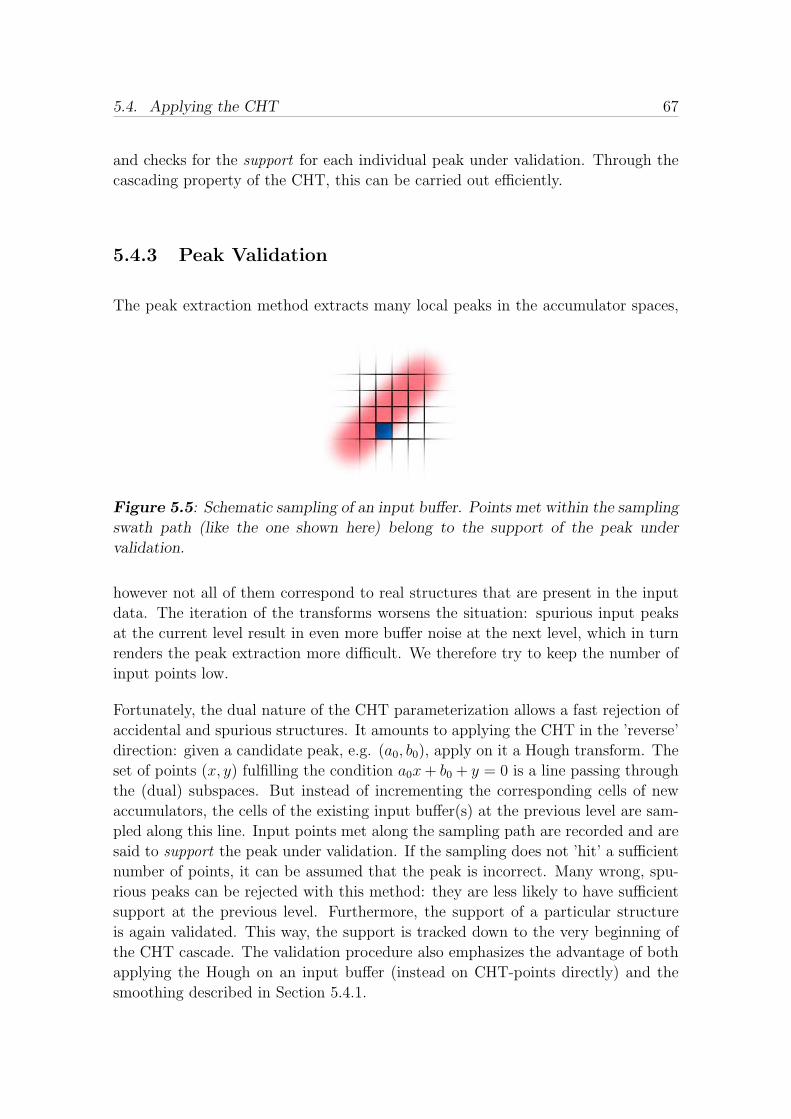
5.4. Applying the CHT 67
and checks for the support for each individual peak under validation. Through the
cascading property of the CHT, this can be carried out efficiently.
5.4.3 Peak Validation
The peak extraction method extracts many local peaks in the accumulator spaces,
Figure 5.5: Schematic sampling of an input buffer. Points met within the sampling
swath path (like the one shown here) belong to the support of the peak under
validation.
however not all of them correspond to real structures that are present in the input
data. The iteration of the transforms worsens the situation: spurious input peaks
at the current level result in even more buffer noise at the next level, which in turn
renders the peak extraction more difficult. We therefore try to keep the number of
input points low.
Fortunately, the dual nature of the CHT parameterization allows a fast rejection of
accidental and spurious structures. It amounts to applying the CHT in the ’reverse’
direction: given a candidate peak, e.g. (a0, b0), apply on it a Hough transform. The
set of points (x, y) fulfilling the condition a0x + b0 + y = 0 is a line passing through
the (dual) subspaces. But instead of incrementing the corresponding cells of new
accumulators, the cells of the existing input buffer(s) at the previous level are sam-
pled along this line. Input points met along the sampling path are recorded and are
said to support the peak under validation. If the sampling does not ’hit’ a sufficient
number of points, it can be assumed that the peak is incorrect. Many wrong, spu-
rious peaks can be rejected with this method: they are less likely to have sufficient
support at the previous level. Furthermore, the support of a particular structure
is again validated. This way, the support is tracked down to the very beginning of
the CHT cascade. The validation procedure also emphasizes the advantage of both
applying the Hough on an input buffer (instead on CHT-points directly) and the
smoothing described in Section 5.4.1.

68 Chapter 5. Basic Technologies II: The Cascaded Hough Transform
5.5 Example
Here we illustrate how the mechanism of the CHT is applied to analyze a set of
points is for its spatial layout. In particular, we are interested if vanishing points
can be detected for the situation shown in Figure 5.6. Note that we come to the
general strategy for the detection of fixed structures in Chapter 7. For the moment,
two successive applications of the Hough transform do the job. A first transform
yields collinear arrangements among the points under investigation, and a second
one finds those locations where collinear structures intersect, i.e. vanishing points.
Subspace 1
-1 +1
-1
+1
Figure 5.6: A cluster of affinely invariant neighbourhoods (left) whose centerpoints
are used as input to the CHT. Right: the input points shown in the CHT coordinate
frame.
We start with a cluster of affinely invariant neighbourhoods (Figure 5.6 left) whose
centerpoints are used as input for the CHT. Figure 5.6 (right) shows the cluster
centerpoints as CHT-points in the first subspace. Next, the Hough transform is
applied for a first time, leading to the unfiltered accumulators shown in the top row
of Figure 5.7. The middle row shows the resulting local maxima found by the peak
extraction method. The bottom row shows the remaining peaks after the validation.
Figure 5.8 makes the effect of the peak validation apparent in the image. On the left,
all peaks in the middle row of Figure 5.7 are drawn as image lines after conversion
to the image coordinate frame. The same is done for the bottom row of Figure 5.7,
leading to the configuration in Figure 5.8 right. Obviously, most of the lines did not
get beyond the validation stage. Almost all peaks in the second subspace (Figure 5.7,
middle and bottom row) were discarded. However, the remaining lines point indeed
to the principal directions of the floor layout. Note that most of the rejected peaks
of the second subspace conform to the converging vertical lines in Figure 5.8 (left).
Although a meaningful pencil of fixed lines, each of these fixed lines is supported by
only two input points, which is insufficient to be non-accidental.

5.5. Example 69
Subspace 1 Subspace 2 Subspace 3
Subspace 1 Subspace 2 Subspace 3
Subspace 1 Subspace 2 Subspace 3
Figure 5.7: Unfiltered accumulator buffers (subspaces 1,2 and 3) after the first
Hough transform (top row). Middle row: Local maxima obtained by the peak
extraction method described in the text. Bottom row: Remaining peaks after the
validation routine in Section 5.4.3 was applied. Darker peaks received more votes
than brighter ones.

70 Chapter 5. Basic Technologies II: The Cascaded Hough Transform
Figure 5.8: Collinear structures among the neighbourhood center points before
(left) and after application of the peak validation routine (right).
The peaks shown in the bottom row of Figure 5.7 now serve as input for a next
Hough. This second transform picks up collinear peaks from the first Hough, which
Subspace 1 Subspace 2 Subspace 3
1
2
3
Figure 5.9: Resulting accumulator buffers after the second Hough transform. The
three peaks that correspond to common intersection points of collinear structures
(vertices of pencils of fixed lines) are the ones emerging in the second subspace
(middle, marked with a circle).
correspond to intersection points of collinear structures among the neighbourhood
centers in the image. The output of the second Hough is shown in Figure 5.9,
with vanishing point candidates in the second subspace. The original input points
re-emerge as peaks in the first subspace, but they are not further considered; see
Chapter 7 for details. Figure 5.10 shows the position of two of the three peaks in
the image coordinate frame, together with their contributing lines.

5.6. Discussion 71
2
13
Figure 5.10: The line intersections (peaks 1 and 3 from Figure 5.9) shown in
the image coordinate frame, together with their supporting lines, i.e. the collinear
structures that contributed to the peaks. The proximity to the origin of peak 2
translates to a location far beyond the image boundaries.
5.6 Discussion
The cascaded Hough transform is an efficient tool for the detection of spatial struc-
tures. It rests on the premise of the point-line duality, which enables the application
of one Hough transform on the output of a previous one. The CHT offers advan-
tages to alternative fitting techniques such as RANSAC, but it should be mentioned
that there are some computational drawbacks and open questions as well. In the
following, we shortly take a closer look at them.
5.6.1 Accuracy vs. Resolution
In principle, the accuracy of the CHT output (point/line parameters) can be well
adapted to the specific needs at hand. Accuracy is primarily adjusted via the size of
the accumulator buffers. A high grade of accuracy is certainly desirable, however this
is at the cost of computation time and storage requirements. While it is generally
true that modern desktop computers are much more powerful than in the early years
of the Hough transform (1960’s), too large accumulator sizes still cause additional
computational expenses.
In our experiments, we used fixed accumulators buffers of size 401 × 401 pixels,
which has proven appropriate for normal images.
5.6.2 Computational Complexity
Hough transforms are generally known to be computationally rather expensive. In
our situation, the computational complexity is highly dependent on the particular

72 Chapter 5. Basic Technologies II: The Cascaded Hough Transform
image, especially on the number of input points. The most expensive part is not
the Hough transform per se, but the extraction of the peaks. As an unsurprising
rule of thumb, the more ’noise’ present in the Hough spaces, the more time the peak
extraction needs.
5.6.3 Peak Extraction
Plenty of room is available for optimization when it comes to the extraction of peaks.
Some ideas that we consider to be promising:
Currently, each CHT subspace is treated in isolation during the peak extraction
process. This is a drawback for peaks very close to the borders of a subspace:
trailing edges might well extend into adjacent subspace(s). A peak extraction
mechanism that does not stop at the boundaries might improve accuracy and
robustness.
In our experiments, we used accumulators of fixed size. However, a system that
incorporates multiple resolutions might help to better ’divide the chaff from
the wheat’: Similar to scale-space approaches, peaks that really correspond
to important structures can be traced across multiple resolutions. Based on
our observations, not so much the absolute height of a peak is of importance,
rather its local neighbourhood. A smaller, isolated peak is more likely to corre-
spond to a non-accidental, meaningful structure than a larger one immediately
surrounded by others. Similar observations were reported by [Liu and Collins
2000] for the extraction of peaks in autocorrelation functions. Although we
do apply a separate peak evaluation technique that helps in reducing noise,
not all incorrect ones can be rejected that way. We therefore think that the
tracking of peaks across multiple resolutions is a promising approach to keep
only relevant structures, however a tradeoff must be found between different
resolutions and the resulting increase in computation time.
5.6.4 Alternative Parameterization
A slope-intercept line parameterization that is equally symmetric with respect to
(a, b) and (x, y) is
ax + by + 1 = 0 (5.14)
This parameterization offers the additional advantage that it is closely related to the
classical equation using homogeneous coordinates ax+by+cz = 0. As a consequence,
a line-corresponding CHT-point (a, b, l) can be converted to its homogeneous form
in a similar way as point-corresponding CHT-points, which directly yields the image-
line parameters (a, b, c) according to the classic parameterization ax + by + cz = 0.

5.7. Summary and Conclusion 73
5.7 Summary and Conclusion
The CHT allows the application of a Hough transform on the output of a previ-
ous Hough transform through a symmetric slope-intersect parameterization of lines.
This way, one can detect collinear structures, intersection points of collinear struc-
tures, collinear configurations of intersection points etc.
Since both (a, b) and (x, y) are unbounded, the entire parameter space is split into
three bounded subspaces. Points and lines in the image can be represented as points
in CHT-subspaces. We introduced the concept of a CHT-point to make the various
conversions between the image and the CHT coordinate frames.
Peaks in the CHT subspaces are extracted using a sort of non-maximum suppression,
followed by a peak-validation routine with the goal to reject wrong and spurious
peaks at the very beginning.
Of course, all kinds of refinements are possible, such as an in-depth analysis of the
effects of the resolution of the parameter spaces and trade-offs thereof, or improve-
ments of the peak extraction technique. Finally, an alternative line slope-intersection
parameterization that also fully exploits the point/line duality is possible as well.


6Detection of Repetitions
After having dealt with the basic technologies in the previous two chap-
ters, we can now turn the attention to the actual grouping process. As
mentioned in the introductory part of this report, the entire grouping
process consists of two principal steps. First, we look for repetitions in
the image, thereby using the affinely invariant neighbourhoods. The second step
then analyzes the spatial configuration of the found repetitions through the use of
the cascaded Hough transform. The most important aspect here is that the two
steps are carried out without the use of extensive combinatorics.
This chapter deals with the detection of repetitions irrespective of their regularity
and is organized as follows. After a short introduction, the description of affinely
invariant neighbourhoods by means of moment invariants is explained. The second
section describes how affinely invariant neighbourhoods can be compared. Next, in
Section 6.4, a matching technique is proposed that looks for clusters of invariant
neighbourhoods in the feature space. Section 6.5 demonstrates the entire process
with a real example. Section 6.6 discusses some aspects of this strategy, and Sec-
tion 6.7 concludes this chapter.
6.1 Introduction
Here, we focus on the detection of small, repeating planar patches, in particular the
affinely invariant neighbourhoods described in Chapter 4. These features are more
general than the lines, line intersections and fixed-sized patches used by others (e.g.[Leung and Malik 1996, Schaffalitzky and Zisserman 1998]). Moreover, the specific
kind of features to be used in an individual image is not selected beforehand by the
user of the system.
We simply run each type of neighbourhood extractor described in Chapter 4 on each
image. The local character of these neighbourhoods improves the robustness of the
system to occlusions, while the invariance to pattern pose and illumination changes
75

76 Chapter 6. Detection of Repetitions
makes it possible to detect the repetition under oblique viewpoints and non-uniform
illumination.
The fact that only invariance under affine geometric deformations is considered may
seem to contradict the aim of dealing with perspective distortions. This restriction
is acceptable in practice though, since the neighbourhoods themselves are rather
small and affinities are a good model for the perspective deformations on such a
local scale. Further, less local steps of the grouping process will deal with the full
perspective effects.
Simplifying further to similarity- or Euclidean transformations is unacceptable for
the kind of images we want to work with. Look for instance at the example of a
tiled floor shown in Figure 1.1. Tiles on the left cannot be mapped onto the tiles on
the right of the figure simply by translation, rotation and adjustment of scale. An
affine transformation, however, is well suited for this task.
In the next section, we explain in more detail how the affinely invariant neighbour-
hoods can be characterized in an invariant way again. This invariant characteriza-
tion is essential for finding similar neighbourhoods under the considered group of
transformations.
6.2 Invariant Description
The techniques presented in Chapter 4 allow the delineation of local, affinely invari-
ant neighbourhoods. With them, local, affine invariants, computed based on the
corresponding support independent of the viewpoint and illumination, can be ex-
tracted. Such invariants are indispensable for an efficient matching of local features
even under strong perspective distortions. As in the neighbourhood extraction step,
we consider invariance both under affine geometric changes and linear photometric
changes (see Equation (4.1) in Chapter 4) in each of the three colorbands.
Each neighbourhood is characterized by a feature vector of moment invariants. The
sole exception are the homogeneous neighbourhoods (see Section 4.2.1). These cover
purely homogeneous patches, which is a rather degenerate case for moments (noise).
For this situation, we use average color ratios for their characterization, to be at
least partially invariant against illumination changes.
The moments we use are generalized color moments [Mindru et al. 1999b]. These
moments integrate powers of the image coordinates and the intensity information
over a neighbourhood:
Mabcpq =
∫∫Ω
xpyq[R(x, y)]a[G(x, y)]b[B(x, y)]c dxdy (6.1)
6.2. Invariant Description 77
with order p+ q and degree a+ b+ c. In fact, they implicitly characterize the shape,
the intensity and the color distribution of the underlying neighbourhood pattern in
a uniform manner. Moment invariants use all information available on a local scale
(geometry, texture and color).
6.2.1 Generic Affinely Invariant Feature Vectors
Several sets of feature vectors have been tested during the work. The first set of
affine moment invariants is also the most generic one, as it can be used for any kind
of affinely invariant neighbourhood, in contrast to the other set (explained in Sec-
tion 6.2.2) that exploits some special properties of specific types of neighbourhoods.
The first set of the more generic invariants make up a feature vector that is composed
of 18 moment invariants. These are invariant functions of moments up to the first
order and third degree. In [Mindru et al. 1999b], it has been proven that the 18
invariants form a basis for all invariants under the considered group of geometric
and photometric transformations involving this kind of moments. An overview of
all 18 invariants is given in Table 6.1.
The reason why these expressions are so complex is that they also take the photo-
metric transformations fully into account, i.e. both a scaling and an offset for each
spectral band. As a result, it is hard to give a physical interpretation. Nevertheless,
the meaning of the 18 moment invariants listed in Table 6.1 can be summarized as
interactions of areas, center of gravities (weighted with one or more colorbands),
correlations of colorbands, relative positions of center of gravities weighted with two
different colorbands and several combinations thereof. By combining geometric with
photometric information, the compensation for illumination changes gets more and
more difficult, hence the growing complexity of the expressions. For a more detailed
interpretation, we refer to [Mindru et al. 1999b, Tuytelaars 2000].
6.2.2 Normalized Feature Vectors
The feature vector presented in the previous section is generally applicable to any
type of affinely invariant neighbourhood. The advantage is that this allows to treat
all neighbourhoods in the same way, and new neighbourhoods types can easily be
added.
However, sometimes knowledge about the neighbourhood extraction can be ex-
ploited to derive simpler invariant expressions with lower order moments and hence
resulting in more stable feature descriptions. This can be achieved by normalizing
the neighbourhood against such transformations.

78 Chapter 6. Detection of Repetitions
Table 6.1: Moment invariants used for comparing the patterns within an invariant
neighbourhood.
SR12 =
M20010 M100
01 M00000 −M200
10 M10000 M000
01 −M20001 M100
10 M00000
+M20001 M100
00 M00010 + M200
00 M10010 M000
01 −M20000 M100
01 M00010
2
(M00000 )2
[M200
00 M00000 − (M100
00 )2]3
D1RG12 =
M10010 M010
01 M00000 −M100
10 M01000 M000
01 −M10001 M010
10 M00000
+M10001 M010
00 M00010 + M100
00 M01010 M000
01 −M10000 M010
01 M00010
2
(M00000 )4
[M200
00 M00000 − (M100
00 )2] [
M02000 M000
00 − (M01000 )2
]
D2RG12 =
(M00000 )2M100
10 M02001 −M000
00 M10010 M000
01 M02000
−2M00000 M010
01 M01000 M100
10 + 2M00001 (M010
00 )2M10010
−M00000 M000
10 M10000 M020
01 + 2M00010 M010
00 M10000 M010
01
−(M00000 )2M100
01 M02010 + M000
00 M10001 M000
10 M02000
+2M00000 M010
10 M01000 M100
01 − 2M00010 (M010
00 )2M10001
+M00000 M000
01 M10000 M020
10 − 2M01010 M100
00 M00001 M010
00
2
(M00000 )4
[M200
00 M00000 − (M100
00 )2] [
M02000 M000
00 − (M01000 )2
]2
inv[1] = SR12
inv[2] = SG12 (similar)
inv[3] = SB12 (similar)
inv[4] = DRG02 =
[M11000 M000
00 −M10000 M010
00 ]2
[M20000 M000
00 − (M10000 )2] [M020
00 M00000 − (M010
00 )2]inv[5] = DGB
02 (similar)
inv[6] = DBR02 (similar)
inv[7] = D1RG12
inv[8] = D1GB12 (similar)
inv[9] = D1BR12 (similar)
inv[10] = D2RG12
inv[11] = D2GB12 (similar)
inv[12] = D2BR12 (similar)
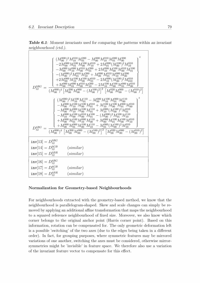
6.2. Invariant Description 79
Table 6.1: Moment invariants used for comparing the patterns within an invariant
neighbourhood (ctd.).
D3RG12 =
(M00000 )2M010
10 M20001 −M000
00 M01010 M000
01 M20000
−2M00000 M100
01 M10000 M010
10 + 2M00001 (M100
00 )2M01010
−M00000 M000
10 M01000 M200
01 + 2M00010 M100
00 M01000 M100
01
−(M00000 )2M010
01 M20010 + M000
00 M01001 M000
10 M20000
+2M00000 M100
10 M10000 M010
01 − 2M00010 (M100
00 )2M010010
+M00000 M000
01 M01000 M200
10 − 2M10010 M100
00 M00001 M010
00
2
(M00000 )4
[M200
00 M00000 − (M100
00 )2]2 [
M02000 M000
00 − (M01000 )2
]
D4RG12 =
(M00000 )2M100
10 M11001 −M000
00 M10010 M000
01 M11000
−M00000 M100
10 M10000 M010
01 + M10010 M100
00 M00001 M010
00
−M00000 M000
10 M10000 M110
01 + M00010 (M100
00 )2M01001
−M00010 M100
00 M01000 M100
01 − (M00000 )2M100
01 M11010
+M00000 M100
01 M00010 M110
00 + M00000 M100
01 M10000 M010
10
+M00000 M000
01 M10000 M110
10 −M00001 (M100
00 )2M01010
2
(M00000 )4
[M200
00 M00000 − (M100
00 )2]2 [
M02000 M000
00 − (M01000 )2
]inv[13] = D3RG
12
inv[14] = D3GB12 (similar)
inv[15] = D3BR12 (similar)
inv[16] = D4RG12
inv[17] = D4GB12 (similar)
inv[18] = D4BR12 (similar)
Normalization for Geometry-based Neighbourhoods
For neighbourhoods extracted with the geometry-based method, we know that the
neighbourhood is parallelogram-shaped. Skew and scale changes can simply be re-
moved by applying an additional affine transformation that maps the neighbourhood
to a squared reference neighbourhood of fixed size. Moreover, we also know which
corner belongs to the original anchor point (Harris corner point). Based on this
information, rotation can be compensated for. The only geometric deformation left
is a possible ’switching’ of the two axes (due to the edges being taken in a different
order). In fact, for grouping purposes, where symmetric features may be mirrored
variations of one another, switching the axes must be considered, otherwise mirror-
symmetries might be ’invisible’ in feature space. We therefore also use a variation
of the invariant feature vector to compensate for this effect.

80 Chapter 6. Detection of Repetitions
inv[1] =M110
00
M00000
inv[2] =M011
00
M00000
inv[3] =M101
00
M00000
inv[4] =M100
10
M10000
inv[5] =M010
10
M01000
inv[6] =M001
10
M00100
inv[7] =M100
01
M10000
inv[8] =M010
01
M01000
inv[9] =M001
01
M00100
inv[10] =M100
11
M10000
inv[11] =M010
11
M01000
inv[12] =M001
11
M00100
inv[13] =M100
20
M10000
inv[14] =M010
20
M01000
inv[15] =M001
20
M00100
inv[16] =M100
02
M10000
inv[17] =M010
02
M01000
inv[18] =M001
02
M00100
Table 6.2: Moment invariants used for comparing the patterns within a
parallelogram-shaped invariant neighbourhood after normalization of the neighbour-
hood to a reference square.
In this way, the affine transformations have been completely compensated for. In
fact, the normalization corresponds to using the points p, p1 and p2 as an affine
basis, and describing the color and intensity profile with respect to this basis.
We also normalize against the photometric changes. However, this cannot be achieved
by exploiting some extra knowledge about the region extraction. Instead, the nor-
malization is directly based on the intensity profile itself, by replacing each intensity
value I by I ′ = aI + b with a and b such that the average intensity is 128 with a
spread of the intensities of 50.
For an overview of the invariants used in this case, see Table 6.2. As all transfor-
mations have been compensated for through normalization, the invariants become
much simpler now. In fact, any measurement in the normalized reference neigh-
bourhood can be used as an invariant. The reason why we stick to moments is that
they are quite robust to noise.
Note that the invariants in Table 6.2 do not necessarily form a basis. Actually, they
were selected rather ad hoc based on their physical interpretation. inv[1] to inv[3]
are related through the correlation between two colorbands. inv[4] to inv[6] and
inv[7] to inv[9] are the x− and y−coordinates respectively of the centers of gravity
weighted with one colorband, while inv[10] to inv[18] are combinations of higher
order moments.

6.2. Invariant Description 81
Normalization for Intensity-based Neighbourhoods
Using the intensity-based extraction method results in elliptic neighbourhoods. A
similar normalization as for the geometry-based, parallelogram-shaped neighbour-
hoods can be applied, this time using a circular reference neighbourhood instead.
However, there remains one degree of freedom to be determined, namely the orien-
tation of the underlying color or intensity profile within the circular reference neigh-
bourhood. The invariants used in this case need to be rotation-invariant. Again,
normalization against illumination changes is applied as well.
inv[1] =M110
00
M00000
inv[2] =M011
00
M00000
inv[3] =M101
00
M00000
inv[4] =
√√√√√ (M10010 M000
00 )2 + (M00010 M100
00 )2 + (M10001 M000
00 )2
+ (M00001 M100
00 )2 − 2 M10010 M000
00 M00010 M100
00
−2 M10001 M000
00 M00001 M100
00
M10000 M000
00
inv[5] = (similar)
inv[6] = (similar)
inv[7] =
√M100
20 (M00000 )2 − 2M000
10 M10010 M000
00 + M10000 (M000
10 )2
+M10002 (M000
00 )2 − 2M00001 M100
01 M00000 + M100
00 (M00001 )2
M10000 (M000
00 )2
inv[8] = (similar)
inv[9] = (similar)
Table 6.3: Moment invariants used for comparing the underlying intensity and
color information within an elliptic invariant neighbourhood after normalization to
a reference circular neighbourhood.
Table 6.3 summarizes the invariants for this case. Only 9 invariants are given here
and were used in the experiments, although it is certainly possible to find more by
combining several colorbands and using second order moments.
inv[1] to inv[3] are identical to the corresponding invariants for the geometry-
based, normalized neighbourhoods (representing the correlation between several
colorbands). inv[4] to inv[6] are the distances between the center of gravity of the
neighbourhood weighted with one colorband and the center point of the neighbour-
hood, while inv[7] to inv[9] correspond to the weighted average squared distances
to the center of the neighbourhood (xm, ym), i.e.
inv[7] =
√∫∫[(x− xm)2 + (y − ym)2]R(x, y) dxdy∫
R(x, y) dxdy

82 Chapter 6. Detection of Repetitions
where R(x, y) denotes the intensity function of the red color band.
Color vs. Grayscale
Whenever color information is available, it is highly recommended to use it for the
invariant neighbourhood description. As opposed to grayscale images, the three
spectral bands constitute additional sources of information, although they are of-
ten not independent as the different bands are correlated. Nevertheless, different
neighbourhoods are easier to discriminate in the feature space. In case of grayscale
images, only the single-banded invariants can be used, which drastically reduces the
number of invariants of second order and first degree (see Table 6.1) without nor-
malization. This is clearly insufficient for an efficient distinction of neighbourhoods.
Alternative ways for the construction of more invariants (e.g. higher order and/or
degrees) are possible (see [Mindru et al. 1998]). In this thesis, though, only color
images have been used for the experiments.
6.3 Neighbourhood Comparison
In grouping, comparison techniques play an essential role, and a wealth of such
techniques exist. Basically, a comparison method yields a similarity (or dissimilarity)
measure given two features. Depending on the features to compare and the context
of the application, some comparison methods are better suited than others. In the
context of efficient grouping, with usually a large number of features (i.e. affinely
invariant neighbourhoods) to inspect, comparison must be performed with minimal
computational effort.
In the first place, we compare affinely invariant neighbourhoods through their fea-
ture vectors. Repetitive neighbourhoods have similar feature vectors close to one
another in the feature space, and identifying such clusters there is exceedingly more
efficient than a direct, pixel-wise search on the neighbourhood contents. Once can-
didates for repetitions have been found in the feature space, we make an additional
cross-correlation check of their intensity patterns for the reasons mentioned in Sec-
tion 6.3.2.
Whatever comparison techniques and similarity measures are applied, we only com-
pare affinely invariant neighbourhoods of the same type, that is neighbourhoods that
were extracted with the same method. Comparing geometry-based, parallelogram-
shaped neighbourhoods to intensity-based, elliptical ones is pointless even on in-
tuitive grounds. Treating all parallelogram-shaped neighbourhoods in the same
manner is problematic as well, because different extraction methods are involved

6.3. Neighbourhood Comparison 83
for the individual neighbourhoods. Hence, to better model the properties of par-
ticular neighbourhood types and their corresponding invariant feature vectors, only
neighbourhoods of the same type are compared.
6.3.1 Feature Vector Comparison
In theory, two feature vectors computed over corresponding neighbourhoods, with
one of them subject to an affine transformation and/or illumination change, should
be identical due to their invariant nature. In practice, though, they will never be
completely equal due to noise, discretization errors and/or misalignments.
Another source of errors are deviations from the model used to approximate the geo-
metric and photometric relations among affinely invariant neighbourhoods. Remem-
ber that we assumed affine geometric deformations and linear photometric changes.
These models are not adequate if there are strong perspective distortions in the
image, if the surface is not completely planar, if patches are partially occluded or
if there are strong specular reflections. In particular, specular reflections can ren-
der the intensity profile of two neighbourhoods completely different, thus making
it impossible to match them. Specular reflections might indeed be quite common
in images of e.g. man-made repetitions (think of the facade of a building with re-
peating windows on a nice day with the sun reflecting on the windows). However,
as this mostly occurs occasionally and on a local scale, this case can safely be ne-
glected. The other deviations are usually small, such that two feature vectors are
still relatively close to one another. In grouping, especially when dealing with a
large number of repetitions, a miss of a few matches can be coped with.
Mahalanobis Distance
The problem we face is the selection of a distance measure between two multi-
dimensional feature vectors to quantify their similarity, i.e. to find out whether two
feature vectors represent two repeating instances of the same neighbourhood. The
spread or variation of their different components might be totally different, which
clearly disqualifies the Euclidean distance as a similarity measure. The variance
of one invariant might be several orders of magnitude larger than the variance of
another invariant. At the same time, several invariants might be correlated as well.
The Mahalanobis distance is a better similarity measure in this case, as it correctly
takes into account this different variability of the elements of the feature vector.
The Mahalanobis distance between two vectors x1 and x2 is given as follows:
dM(x1,x2) =√
(x1 − x2)>Σ(x1 − x2) (6.2)

84 Chapter 6. Detection of Repetitions
where Σ is the covariance matrix. Σi,i represents the spread (i.e the variance σ2)
of the i’th element of the feature vector and Σij/√
ΣiiΣjj, (i 6= j) the correlation
between the i’th and j’th component.
Achieving maximum Separability
The occurrence of multiple repetitions (of different features) in the image corre-
sponds to multiple clusters in the feature space. If clusters form well separated,
compact entities, their automatic identification is certainly eased.
At the same time, one is also interested in a reduction of the dimensionality of the
feature space, be it e.g. for visualization or a cut-down in computational complexity.
However, a lower-dimensional space is in vain if the separability of the original
features is lost. It is therefore of importance that well separated features remain
well separated in the reduced space.
Reasonable distance measures involving the Mahalanobis distance greatly depend on
the covariance matrix Σ. The crux of the matter is that Σ strongly depends on the
degree of viewpoint and illumination change, and last but not least on the underlying
intensity profile of the affinely invariant neighbourhood. As a consequence, it is not
straightforward to obtain a good estimate Σ.
In most cases, the variability of a single feature over different viewing conditions
is hardly related to the overall variability of that feature. Some features may be
very stable to image noise or changing viewing conditions, resulting in a low intra-
class variability, while they still vary a lot between different neighbourhoods due to
the different intensity profile. Other features, especially those using higher order
moments, are significantly less discriminative, as they are more sensitive to noise,
misalignment of the neighbourhood or deviations from the model, regardless of the
overall variability of the feature.
Actually, the optimal feature is a feature with a high discriminative power, i.e.
the combination of a high variability between neighbourhoods covering different
patterns with a low variability of the same neighbourhood over different viewing and
illumination conditions. In contrast to techniques like e.g. the principle component
analysis, a linear discriminant analysis (LDA) is well suited for this task, as it
maximizes the ratio of the inter-class to the intra-class variabilities through two
consecutive coordinate transformations.
The LDA rests on the premise of the less strict common covariance matrix assump-
tion. It is assumed that all neighbourhoods share the same intra-class statistics
(independent of the color or intensity profile). However, these statistics can be dif-
ferent from the overall, inter-class statistics. It has been shown that, if the number
of training samples is small, this assumption leads to higher classification accuracy,

6.3. Neighbourhood Comparison 85
even if the covariance matrix of each class greatly differs [Friedman 1989]. Ap-
pendix A illustrates the LDA as applied in this thesis in more detail and shortly
explains how we obtained estimates for neighbourhood-specific covariance matrices.
6.3.2 Correlation-based Comparison of Affinely
Invariant Neighbourhoods
Apart from comparing the invariant feature vectors of two neighbourhoods, one can
also directly compare the pixel intensities in the two neighbourhoods by computing
the cross-correlation. The definition of the normalized cross-correlation is given by
dC =
∑i
∑j
[I(x + i, y + j)− I
] [I ′(x′ + i, y′ + j)− I ′
]√∑
i
∑j
[I(x + i, y + j)− I
]2∑
i
∑j
[I ′(x′ + i, y′ + j)− I ′
]2(6.3)
with (x, y) and (x′, y′) the corresponding pixels in the first respectively the sec-
ond neighbourhood, I(x, y) and I ′(x′, y′) the respective intensities and I and I ′ the
average intensities.
The cross-correlation as such is sensitive even to small distortions. It assumes that
the pixel corresponding to (x + i, y + i) is located at (x′ + i, y′ + i), which is only
the case for a pure two-dimensional translation. Therefore, affine shape normal-
ization is required, that is the original neighbourhoods must be transformed to a
unit square (parallelogram-shaped neighbourhoods) and circular reference neigh-
bourhood (elliptical-shaped neighbourhoods) first. In this way, the geometric de-
formations are compensated for, except for the rotational component of elliptical
neighbourhoods, which is found by maximizing the cross-correlation.
dC can be interpreted as a similarity measure with values always ranging from -1 to
+1. It is equal to ±1 if and only if the two intensity patterns are related by a linear
relation. The lower the absolute value of dC, the less correlated the patterns are. In
the rest of this text, we simply use the term ’cross-correlation’ when referring to the
normalized cross-correlation.
Cross-correlation is a more powerful measure than the Mahalanobis distance. How-
ever, it is by far not as efficient than the Mahalanobis distance due to the compu-
tational complexity. In spite of the larger computational effort, we combine both
methods for the detection of repetitions, as explained in more detail in Section 6.4.
6.3.3 Other Comparison Methods
The cross-correlation-based comparison of two neighbourhoods is based on the as-
sumption of linear changes in image intensities. Indeed, the cross-correlation directly

86 Chapter 6. Detection of Repetitions
measures the linear dependency of two intensity profiles. Similarly, the invariants
used for the Mahalanobis-based comparison also assume a linear model for the inten-
sity changes. However, as shown in [Tuytelaars 2000], the underlying linear model
is not always exact.
The modeling of illumination effects is still an open area of research, and previous
publications are mixed about their conclusions concerning intensity changes and
achieving illumination invariance. Invariants based on a more complex, full affine
illumination model (in combination with perspective, geometric deformations) have
been developed recently [Mindru et al. 2001]. The authors report a gain of 10% in
recognition performance (for natural images), thereby confirming the superiority of
the new, but more complex invariants for such images.
Other measures based on maximum likelihood can correctly deal with non-linear and
unmodelled intensity transformations. However, these are not yet implemented in
our system, but might offer promising alternatives for further improvements.
Mutual Information
Mutual information allows to measure the similarity between two neighbourhoods
without a specific model for the relationship between corresponding intensity values.
This is a technique based on information theory and was introduced by Viola and
Wells [Viola and Wells 1997] in the context of registration and recognition. Mutual
information is measured as follows:
I(I, J) =∑
i
∑j
log
(p(i, j)
p(i)p(j)
)(6.4)
with p(i) the probability of intensity i in image I, p(j) the probability of intensity
j in image J and p(i, j) the joint probability of intensity i in image I and intensity
j in image J . Basically, this measure expresses the idea that the color or intensity
profile of one neighbourhood should be predictable to a high degree based on the
color or intensity profile of the other neighbourhood. The pure existence of this
statistical relationship suffices to obtain high scores with this measure, without a
model for the exact form of the relationship. Mutual information measures the
general dependence, while correlation quantifies the linear dependence between two
neighbourhoods.
Correlation Ratio
As an alternative to statistical relationships, the correlation ratio tests for the exis-
tence of a functional relationship [Roche et al. 1999]:
η2(I, J) = 1− V arI − φ(J)V arI
(6.5)

6.4. Matching / Clustering 87
with φ(J) the least square optimal non-linear approximation of I in terms of J and
V ar. . . the variance of the measure between brackets. Each color or intensity
value in the first neighbourhood is mapped to a color or intensity value in the other
neighbourhood (or, more precisely, a distribution around a single color or intensity
value). The fundamental difference to mutual information is that the correlation
ratio is based on the variance instead of the entropy.
6.4 Matching / Clustering
Once we have extracted the different types of affinely invariant neighbourhoods, we
try to find the repeating patterns by looking for clusters of invariant neighbourhoods
in the feature space. This is the space spanned by the elements of the feature vector
of moment invariants described earlier.
For the rest of the text, we distinguish between large clusters (consisting of more
than 6 neighbourhoods) and small clusters (consisting of anything between 2 and
6 neighbourhoods). To avoid heavy combinatorics, the large clusters (typically be-
longing to periodicities) will sometimes be dealt with in a different manner than the
small clusters (typically belonging to mirror-symmetries and / or point-symmetries).
Large and small clusters translate to regions of high- and low densities in the feature
space, respectively.
The actual matching and clustering goes as follows. For each different type of neigh-
bourhood (e.g. geometry-based with curved edges or intensity-based), a separate
feature space is built. To better separate the different clusters and to reduce the di-
mensionality of the feature space, a linear discriminant analysis is performed. In fact,
a dimensionality reduction is necessary, since an 18-dimensional (9-dimensional) fea-
ture space with only a few hundreds of datapoints (feature vectors) is too sparse for
representative statistics.
Clusters are then identified in this reduced space through a non-parametric density
estimation using an unimodal Gaussian kernel. The choice of the with σ of the con-
volution kernel is usually a crucial issue in density estimation [Scott 1992]. Setting
the value for σ too large can be interpreted as an oversmoothing of the data, which
prevents important structures from becoming ’visible’. Too small a value, on the
other hand, results in too many, fine-grained density peaks. Since the distribution of
the overall features is unknown, a value for σ has to be set based on the underlying
data. We adapted a method described by [Pauwels and Frederix 1999] to set σ in a
data driven way.
More precisely, given an n-dimensional dataset xi ∈ IRn; i = 1 . . . N, a density
f(x) is obtained by convolving the dataset with the the unimodal density kernel

88 Chapter 6. Detection of Repetitions
Kσ(x):
f(x) =1
N
N∑i
Kσ(x− xi) (6.6)
where σ is the (beforehand) unknown size-parameter for the kernel, measuring its
spread. In particular, the unimodal (rotation-invariant) Gaussian is given by
Kσ(x) =
(1
2πσ2
)n/2
e−‖x‖2/2σ2
(6.7)
The spread parameter σ is now taken proportional to the average radius of the ball
that encloses the k nearest neighbours of a datapoint. This has the advantage that
σ is completely determined by the data and scales with the size and range of the
dataset. The number k of nearest neighbours is fixed to be one percent of the total
number of datapoints, but with a minimum of k = 10, i.e.
k = max0.01N, 10 (6.8)
The neighbourhood with maximum density is then selected as seed for a new cluster
and will be used as a cluster prototype. Other neighbourhoods are added to the
cluster if they are within a predefined distance d from the moving average of the
cluster, provided that they also yield a good score on the cross-correlation test (w.r.t.
the prototype). This is an additional, final test, that has been added to reduce the
number of errors (neighbourhoods belonging to a cluster even though they don’t
cover the same pattern). Here again, the correlation is computed after normaliza-
tion to a square or circular reference neighbourhood. In case of intensity-based,
elliptical neighbourhoods, the correct rotation between the two circular reference
neighbourhoods is determined by maximizing the cross-correlation.
Next, all neighbourhoods belonging to the cluster are removed from the feature
space and the same process is repeated until no more clusters are found.
Parameters
A Mahalanobis distance threshold of d = 3 for two features to be similar has pro-
duced good results. Assuming that the covariance matrix has correctly been es-
timated and that the invariants have a Gaussian distribution, the probability of
not being within this boundary, although the neighbourhoods have correctly been
extracted, is smaller than 5%.
Concerning the dimensionality reduction of the feature space, we have found that a
projection of the feature vectors to the first two principal components corresponding
to the two largest eigenvalues is sufficient without a loss of essential information.
The threshold for the cross-correlation was set to 0.7 in all our experiments.

6.5. Example 89
6.5 Example
Here we show the matching/clustering step with a typical elation example. In order
to avoid scene clutter, we only show one neighbourhood type. The advertising panel
Figure 6.1: The original image (left) and all intensity-based elliptic neighbour-
hoods extracted around intensity extrema. A total of 182 neighbourhoods were
found.
in Figure 6.1 shows a planar repetition of beer cans, and we wish to ’capture’ these
repeating elements in terms of intensity-based, affinely invariant neighbourhoods.
529 intensity extrema led to the extraction of 182 elliptical neighbourhoods (right)
in about 3 seconds.1 The computation of all feature vectors took about 7 seconds,
incl. the transformations needed by the discriminant analysis. The two principal
components of the dataset corresponding to the two largest eigenvalues are shown
in Figure 6.2 after the density estimation, with dark grayvalues indicating high
densities. Density estimation takes less than a second for this example, resulting
in a σ of 1.58 for the convolution kernel. Three isolated regions of higher density
can be spotted. The datapoint with the highest density is located in the second
quadrant and serves as the prototype for the clustering algorithm.
In this part of the feature space, a cluster of 22 neighbourhoods was found in ap-
proximately 3 seconds. The corresponding neighbourhoods are shown in Figure 6.3
left, both in the image and the feature space. After removal of the cluster and a
density re-estimation, the datapoint with the highest density acts as the prototype
again for a new clustering run. This time, the system took approx. 7 seconds to
extract a second cluster of 12 neighbourhoods.
1Sun Ultra 10, 440 MHz. Image size: 700 × 525

90 Chapter 6. Detection of Repetitions
-10 10 201. PC
-15
-10
-5
5
10
2. PC
Figure 6.2: The first two principal components of the feature space after the LDA
transformations and the density estimation. The mean was subtracted from all
datapoints. The grayvalues of the points are proportional to their density values.
The three regions of higher density (darker points) are indeed in agreement to what
a coarse visual inspection would depict as cluster candidates.
6.6 Discussion
Usually a few hundreds of affinely invariant neighbourhoods are extracted per image
(depending on the neighbourhood type and image content), and the corresponding
feature spaces of 18 (9) dimensions are quite sparse such that a reduction in di-
mensionality is appropriate. A crucial point is that the features must keep their
discriminative power in the reduced space, which emphasizes the need for a linear
discriminant analysis.
A LDA results in better separability of clusters by minimizing intra-cluster dis-
tances while maximizing inter-cluster distances. However, this procedure does not
always yield the desired result. This might be the case in situations where only one
cluster is present. The net effect is a disruption of the cluster, with some correct
neighbourhood matches going undetected.
Without the LDA, feature vectors usually occupy a smaller portion of the feature
space, i.e. they are closer to each other. As a consequence, many more datapoints
are within the predefined Mahalanobis distance around the prototype — and not
only those belonging to the cluster. As a result, one might obtain more correct
matches, but at the cost of a tremendous increase in computation time. For an

6.6. Discussion 91
-12 -8 -41. PC
-15
-10
-5
5
2. PC
-12 -8 -41. PC
-15
-10
-5
5
2. PC
Figure 6.3: Top: Two clusters of intensity-based neighbourhoods that have been
found using the clustering method described in Section 6.4 in the image. Bottom:
Enlarged part of the feature space from Figure 6.2 with the two clusters encircled.
The first cluster to the left was removed from the feature space before looking for
the second cluster (right).

92 Chapter 6. Detection of Repetitions
average of about 200 affinely invariant neighbourhoods, the detection of clusters
would be in the range of several minutes (per cluster).
Another issue addresses the question if a re-estimation of densities is necessary after
a cluster has been removed from the feature space. Clearly, the removal of datapoints
affects its overall structure w.r.t the densities. Our experiences have shown that a
re-estimation leads to a faster detection of other clusters (if there are any). To better
explain this effect, imagine a situation similar to the example shown in the previous
section, with a first cluster comparatively larger than a second one. After removal
of the first cluster, datapoints within or close to the region of that cluster, but not
being members of it, still might have larger densities than those points in the second
cluster (without density re-estimation). As a consequence, the search for the second
cluster starts at a wrong location. A re-estimation corrects this effect. We therefore
consider an update of feature densities (after the removal of a cluster) as necessary.
6.7 Summary and Conclusions
A preliminary grouping step is performed with the goal to find similar, small planar
patches, irrespective of their regularity. Through the use of the affinely invariant
neighbourhoods introduced in Chapter 4, similar such neighbourhoods can be found
efficiently by describing each by a feature vector consisting of moment invariants.
This allows the use of indexing techniques, which improves efficiency. Repetitions
are then detected by looking for similar feature vectors in the feature space in
combination with a normalized cross-correlation. Several alternative comparison
methods are presented as well.
A linear discriminant analysis with tracking-based covariance matrices leads to a
substantially better discriminative power of the features, which again contributes to
the overall efficiency.
Repetitive neighbourhoods correspond to clusters in the feature space. A non-
parametric density estimation identifies regions where several feature vectors gather,
and density peaks serve as prototypes for examining their immediate surroundings
w.r.t. a predefined Mahalanobis distance, thereby using the moving average of the
prototype as new cluster candidates are added. Once a cluster has been found and
removed from the feature space, the procedure is repeated.

7Detection of Regularities
Regularities are repetitions of planar patterns in a regular, well defined
spatial arrangement. This implies the existence of certain ’rules’ or
’guidelines’ that make up the entire pattern. Formally, the spatial con-
figuration can be seen as the effect of an underlying mathematical law
responsible for its creation, hence the name regular. And indeed, the general mathe-
matical description of symmetries by transformation groups provides an insight into
the mechanisms that build symmetric patterns.
This chapter deals with the detection of regularities of repeating patterns, that is
the governing mathematical laws. After a brief introduction, in Section 7.2 it is
explained how the cascaded Hough transform introduced in Chapter 5 is applied
to clusters of similar affinely invariant neighbourhoods to extract fixed structure
candidates. Section 7.3 describes the instantiation of planar homology hypotheses,
and Section 7.4, describes a method for their verification. In Section 7.5, some pros
and cons are discussed and Section 7.6 concludes the chapter.
7.1 Introduction
Now that we have found one or several repeating patterns in the image, the goal
is to find the regularities behind them (if there are any). As mentioned earlier, we
assume that the regular repetition of an image pattern can be characterized by a
planar homology. Our goal here is to find that homology.
We recall that the corresponding projectivity H has a line of fixed points and a pencil
of fixed lines. To hypothesize H, we first extract fixed structure candidates. This is
achieved in a non-combinatorial way, using the CHT (see Chapter 5). Next, a single
neighbourhood match suffices to lift the remaining degree of freedom. Why do we
need an additional neighbourhood match ? Remember from Chapter 3 that general
planar homologies have 5 dof, yet the fixed structures lift 4 dof in total. Hence,
an additional point match is needed. The situation is only slightly different in the
93

94 Chapter 7. Detection of Regularities
case of elations. Here, the fixed structures lift 3 dof (the vertex of the pencil lies on
line of fixed points), thus leaving us with one remaining dof, thus the need for an
additional point match.
To sum up, finding a grouping characterized by a general planar homology amounts
to the determination of a transformation with 5 dof. The prior knowledge of the
fixed structures cuts down the complexity of the problem considerably to 1 dof.
However, a system can only benefit from this reduction if no additional, unnecessary
complexity is introduced for the extraction of the fixed structures. In the following,
we explain how this can be achieved efficiently.
7.2 Finding Fixed Structures
The first step in the analysis for regularity comprises the extraction of fixed structure
candidates, and this process has to be carried out efficiently, i.e. without recursing
to combinatorial methods. We propose the use of the CHT to get to the desired
result.
To shortly outline the strategy, we use two procedures for extracting pencils of fixed
lines and lines of fixed points candidates, where each applies the CHT two times
successively. Essentially, both procedures are identical in what they do. Their only
difference is that they act on spaces dual to each other, see Table 7.1.
7.2.1 Candidate Pencils of Fixed Lines
Large Clusters
To find good candidates for pencils of fixed lines, we use the center points of invariant
neighbourhoods belonging to a cluster as input for the CHT. Collinear arrangements
of neighbourhood centers can be detected by applying a Hough transform on these
center points. A second Hough transform applied to the peaks of the output of the
first one yields intersections of straight neighbourhood alignments, i.e. candidates
for pencils of multiple fixed lines.

7.2. Finding Fixed Structures 95
Pencils of fixed lines Line of fixed points
Small Large Small Large
— center points↓ Hough ↓ 0
joinscollineararrangements
—characteristiclines
1
↓ Hough ↓
intersectionsof joins
intersectionsof collineararrangements
Intersections ofcharacteristiclines
intersectionsof character-istic lines
2
↓ Hough ↓collinear con-figurationsof charac-teristic lineintersections
collinear con-figurationsof charac-teristic lineintersections
3
Table 7.1: Strategy for extracting fixed structure candidates working on both large
and small clusters of affinely invariant neighbourhoods. Structures used as input are
printed in a sans-serif font, and their corresponding outputs are printed in boldface.
The numbers in the outermost right column indicate the CHT level numbers.
Small Clusters
For the small clusters, the joins connecting the centers of neighbourhoods belonging
to the same cluster are added as direct input before taking the second Hough.
Adding these lines helps in detecting the vertices of the pencils of fixed lines in case
where there is only a limited number of repetitions (e.g. mirror-symmetries). Adding
lines between pairs of neighbourhood centers seems to undermine our goal of avoiding
combinatorial steps. However, since this measure is restricted to neighbourhoods
belonging to small clusters, relatively few such lines are constructed (maximum 15
lines per cluster).
When applying two successive Hough transforms, the original input will re-emerge
as peaks in the Hough spaces. As a result, the original neighbourhood centers pop
up in the space where we look for pencils of fixed lines. However, since we know
which points have been used as input, these peaks can be identified and ignored for
further processing.

96 Chapter 7. Detection of Regularities
7.2.2 Candidate Lines of Fixed Points
Large Clusters
To detect candidates for lines of fixed points, we apply exactly the same scheme as for
the detection of the pencil of fixed lines candidates, but in the dual spaces. As input
for the first Hough transform, we use characteristic lines of the neighbourhoods.
These are sides and diagonals of the parallelogram-shaped neighbourhoods, and a
photometric invariant variant of the axes of inertia of the elliptical neighbourhoods.
In more detail, these axes of inertia can be found by first mapping an elliptic neigh-
bourhood to a circular reference neighbourhood. Next, the major and minor axes are
then extracted as the lines passing through the center O with orientations θmax, θmin
defined by the solution of
tan2 θ +m20 −m02
m11
tan θ − 1 = 0 (7.1)
with mpq the p + q’th order, first degree moment centered of the neighbourhood’s
geometric center. It can be shown that these axes are invariant under both linear
intensity changes and rotation, in the sense that they cover the same part of the
neighbourhood after a rotation. For more details we refer to [Ferrari et al. 2001]. It
must also be mentioned that this problem is ill-conditioned if elliptic neighbourhoods
cover patterns with a perfect rotational symmetry. The resulting axes of inertia can
no longer be used. In such situations, we proceed according to the strategy for
the extraction of pencils of fixed lines (using the centerpoints; see previous section)
and apply the Hough for a third time. This way, fixed structures can be found
when parallelogram-shaped neighbourhoods offer no alternative, like in the situation
shown in Figure 4.10.
By applying a first Hough transform, points where many of these lines intersect can
be detected. A second Hough transform applied to the peaks of the output of the
first one yields collinear arrangements of intersection points. These correspond to
the candidate lines of fixed points.
Small Clusters
Again, for the small clusters, we add some additional input before taking the second
Hough transform. In this case, these are intersections of corresponding characteristic
lines (e.g. intersections of corresponding sides and diagonals of parallelogram-shaped
neighbourhoods). This makes it possible to detect lines of fixed points, even if the
number of repeating patterns is low.
Since we use several input lines for each neighbourhood, spurious peaks will pop up
after applying the Hough transform. Indeed, starting from the sides and diagonals

7.2. Finding Fixed Structures 97
of a parallelogram-shaped neighbourhood, it is obvious that the corners and center
of the parallelogram will be detected as intersection points, although they are not
really of interest to us. The same holds for the elliptical neighbourhoods, where the
neighbourhood centers will be detected as intersection points of the axes of inertia.
These are not the non-accidental intersections we are interested in (since they are
not related to the regularity at all). Hence, they have to be removed before taking
the second Hough transform.
7.2.3 Example
Let us take the image shown in Figure 4.8 as an example. The relevant planar
homologies in this example are the different elations that correspond to translations
from one tile to another in the ground plane. The candidate pencils of fixed lines to
be detected have their vertices in the vanishing points of these translation directions,
while the common line of fixed points corresponds to the horizon line.
Pencils of Fixed Lines
The centers of the neighbourhoods of the floor tile clusters shown in Figure 4.8
were used as input to the CHT to find the candidate vertices of pencils of fixed
lines (top row in Figure 7.1). The middle row of the same figure shows the three
unfiltered subspaces after applying the Hough for the first time (level 1). Peaks in
these spaces correspond to collinear arrangements of neighbourhood centers. Note
that the peaks in the first and especially in the second subspace are again placed in
collinear arrangements. This is because they represent a set of convergent lines.
It is this collinearity of the peaks in level 1 that is detected by the second Hough
transform. The bottom row of Figure 7.1 shows the unfiltered output of this sec-
ond Hough transform. This time, the peaks indicate locations (both inside and
outside the image) where collinear structures intersect. These include the original
input points (the peaks in the first subspace) as well as the vanishing points that
correspond to the pencil vertices. After removal of the re-emerging peaks, only six
candidate vertices for pencils of fixed lines remain. Figure 7.2 shows the candidate
vertices for pencils of fixed lines (except for the one that fell too far outside the im-
age boundaries to be displayed), together with the lines (collinear structures) that
contributed to them.
It should be mentioned here that a cluster of 42 elliptical neighbourhoods was found
as well, with almost circular shapes around the tile centers. The centerpoints of this
cluster coincides very well with a subset of the cluster from Figure 4.8 and yield
indeed two of the candidate pencils shown in Figure 7.2. However, their axes of

98 Chapter 7. Detection of Regularities
First subspace Second subspace Third subspace
leve
l0
leve
l1
leve
l2
Figure 7.1: Detection of the candidate pencils of fixed lines based on the CHT
for the largest cluster found in the image shown in Figure 4.8: the input (centers
of neighbourhoods belonging to one cluster) (top), the three unfiltered subspaces
after applying a first Hough transform (middle), and after applying a second Hough
transform(bottom). Apart from the original input points (in the first subspace),
additional peaks arise in the second and third subspace, that correspond to the
vertices of the pencils of fixed lines.

7.2. Finding Fixed Structures 99
Figure 7.2: The candidate pencils of fixed lines and the most dominant vanishing
line, as detected by the CHT, after conversion to the image coordinate frame. Pencils
of fixed lines are shown together with their vertices (filled circles). Different sizes
indicate different support.
inertia are ill-conditioned and thus inapplicable for the extraction of line of fixed
point candidates.
Lines of Fixed Points
To find the candidate lines of fixed points, the sides and diagonals of the parallelogram-
shaped neighbourhoods of the cluster were used as level 1 input to the CHT. The
top row in Figure 7.3 shows the corresponding input spaces.
After applying a first Hough transform, we obtain the three (unfiltered) subspaces
(level 2) shown in the middle row of the same figure. The most salient peaks (in
the second and third subspaces) correspond to vanishing points 1. Most of the
peaks in the first subspace are removed before taking the second Hough transform,
since they correspond to neighbourhood centers or corners instead of non-accidental
alignments.
Finally, the result of applying a second Hough transform to the peaks of the output
of the previous level is shown in the bottom row. The peaks in the first subspace
(left) correspond to lines that have been used as input two levels before, so they
don’t bring any new information and are rejected as re-emerging peaks. Only the
intersection of the three lines in the third subspace (right) is non-accidental, hence
it is a promising line-of-fixed-points candidate for the regularity of the kitchen floor.
It is also shown in Figure 7.2.
1The fact that the output is so similar to the bottom row of Figure 7.1 is due to the fact thatwe’re dealing with elations, so the vertices of the pencils of fixed lines coincide with the structuresthat contribute to the line of fixed points.

100 Chapter 7. Detection of Regularities
First subspace Second subspace Third subspace
leve
l1
leve
l2
leve
l3
Figure 7.3: Detection of the candidate lines of fixed points based on the CHT
for the largest neighbourhood cluster of the image shown in Figure 4.8. The input
spaces(characteristic lines of the neighbourhoods belonging to the cluster) (top), the
three unfiltered subspaces after applying a first Hough transform (middle), and after
applying a second Hough transform (bottom).

7.3. Finding the Groupings 101
7.3 Finding the Groupings
In order to hypothesize a planar homology (incl. elation) we start by selecting a
good pair of candidate line of fixed points and a candidate pencil of fixed lines.
These are structures that both received many votes by the CHT and to which the
same repeating neighbourhoods have contributed. Once the fixed structures have
been hypothesized, a single pair of repeating neighbourhoods fixes the last remaining
degree of freedom of the planar homology H.
In case of large clusters, only pairs of neighbourhoods close to one another are ex-
amined. These correspond to the smallest distance of a repetition, which intuitively
becomes clear for the example shown in Figure 7.2: a neighbourhood pair close
to one another denotes a translation in the magnitude of one tile. Moreover, we
only consider pairs of neighbourhoods that both contributed to the extraction of
both fixed structures and that can be mapped onto each other by a member of the
subgroup of the projectivities defined by the fixed structures. The peak validation
described in Section 5.4.3 enables a fast identification of neighbourhoods that con-
tributed to a particular fixed structure, because the validation can iteratively be
applied to any CHT level further down. Hence, for each fixed structure candidate,
we can trace down the support until we arrive at the input level (level 0 or 1). From
here, the corresponding neighbourhoods can then easily be identified.
The peak validation yields not only the neighbourhoods that contributed to a fixed
structure, but also imposes a spatial organization on this set with respect to the
subgroup at hand: as an example, the neighbourhoods that contributed to a pencil
of fixed lines must necessarily lie on a fixed line, and the peak validation routine
quickly identifies them.
These measures avoid slipping into combinatorics during the process of hypothesis
instantiation. Note also that the number of planar homology hypotheses to be
validated is much smaller than the number of pairs of close neighbourhoods, since
typically many pairs result in the same hypothesis.
Finally, a hypothesis can be instantiated in practice using Equations (3.3) and (3.4),
resp., by solving for the unknown parameter µ (the remaining dof).
7.4 Hypotheses Validation
Once fixed structures and thus groupings are hypothesized, these need to be verified.
In particular, the planar homology hypotheses need further testing, with a threefold
goal:

102 Chapter 7. Detection of Regularities
Efficiency: The CHT might yield several candidates for fixed structures. As this
leads to a hypothesize-and-verify method, wrong candidates must be rejected
with minimal computational effort.
Extent: Given a hypothesized planar homology, we want to find out exactly the
support in the image for this specific hypothesis, i.e. segment the image into
a consistent and a non-consistent part.
Correctness: From this point onwards perspective effects should be taken fully
into account. Also, by pulling more information from the image, a more accu-
rate estimate of the transformation can be obtained.
These goals are achieved by a region-growing algorithm that compares the original
image to its warped version for conformity based on normalized cross-correlation.
Warped in this context means the pixel-wise transformation of the original image
with the hypothesized planar homology H. An example is shown in Figure 7.4.
Figure 7.4: Semi-transparent overlay of the original image and its warped version.
The hypothesis in this case is a translation of one ’tile-unit’ to the left (elation).
We use the center of the repeating neighbourhoods that contributed to the detection
of the fixed structures as seed points for our region-growing algorithm. The correla-
tion is computed locally for corresponding pixels in both images using a correlation

7.4. Hypotheses Validation 103
window of fixed size. In case the correlation value for pixel pi,j is larger than a
predefined threshold, then pi,j is considered to be in agreement with the hypothesis
H and the same procedure is repeated for the adjacent pixels pi,j−1, pi,j+1, pi−1,j and
pi+1,j. The region growing algorithm stops when there are no candidate pixels left to
be evaluated. The whole procedure is repeated for all remaining centerpoints that
have not fallen inside an already grown region. As a consequence, even disconnected
groupings can be segmented.
To compensate for inaccuracies in the grouping hypotheses and/or imperfect sym-
metries, we allow the correlation window to drift a distance of one pixel starting
from the average displacement at neighbouring pixels. In this way large but gradual
deviations can be compensated for while using a correlation window shift of only
one pixel, which keeps the computation time low. At the same time, we limit the
total drifting distance to half the Euclidean distance between a pixel at (i, j) and
its warped location (i′, j′, 1)> = H(i, j, 1)>, to avoid too large deviations from the
original hypothesis. Allowing the correlation mask to slide gradually has proven
to yield good results in situations where the symmetry in the image is not perfect,
and / or the hypothesized symmetry has noise on it.
For a hypothesized planar homology that is not correct, the correlation value almost
immediately drops below the threshold value, giving very small segmentations that
can easily be rejected. This results in a fast rejection of false hypotheses.
Example (ctd.)
For the example shown in Figure 4.8, we combined the strongest candidate pencil
of fixed lines with the only candidate line of fixed points. From all those neigh-
bourhoods belonging to the cluster, only one planar homology hypothesis emerged,
corresponding to a translation over one ’tile-unit’. We then warped the image ac-
cording to this transformation, as shown in Figure 7.4.
Note how the original floor tiling coincides with its warped version, while the non-
repeating objects seem motion-blurred, like e.g. the dog in the middle and the
drawers to the right. This is exactly what is being detected during the hypothesis
verification stage.
Figure 7.5 shows the resulting segmentation. The part of the image that is not
darkened was found to be consistent with the hypothesized transformation. The
’holes’ in the foreground arise due to the fixed-size correlation window and the
homogeneity of the tiles. Note that the extension of the segmentation over part of
the cupboard at the upper left part of the image is correct: since we are considering
a ’horizontal’ translation, this part of the image is indeed consistent, as can also be
seen from Figure 7.4. The computation time needed to validate this hypothesis was
1 minute and 45 seconds.

104 Chapter 7. Detection of Regularities
Figure 7.5: Validation result (segmentation) of the hypothesis shown in Figure 7.4.
Darker pixels are considered inconsistent with the hypothesized transformation.
7.5 Discussion
7.5.1 Advantages of the CHT
Using the CHT allows many neighbourhoods to contribute to the selection of can-
didate fixed structures right from the start. This reduces the influence of possible
imprecisions in their individual positions, which have a much stronger impact in the
case of RANSAC [Fischler and Bolles 1981] (e.g. used in the work of Schaffalitzky
and Zisserman [Schaffalitzky and Zisserman 2000]).
Another advantage over more heuristic methods like RANSAC is the superior per-
formance with respect to outliers. This is especially the case when the number
of outliers equals the number of inliers. Such situations might cause RANSAC to
increase the computation times for a resulting model (without any guarantees for
correctness), thus becoming prohibitively expensive with respect to computational
complexity.
7.5.2 Parameters
In our experiments, we have used accumulator buffer sizes of 401 × 401 pixels for
each subspace. Concerning the peak validation, a minimum support of three input
points/lines are set as threshold for a peak to be accepted, i.e. to be non-accidental.
A correlation window size of 25 × 25 pixels was used for the validation with a
correlation threshold set to a value of 0.7. To decrease the computation time for
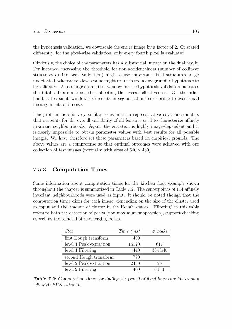
7.5. Discussion 105
the hypothesis validation, we downscale the entire image by a factor of 2. Or stated
differently, for the pixel-wise validation, only every fourth pixel is evaluated.
Obviously, the choice of the parameters has a substantial impact on the final result.
For instance, increasing the threshold for non-accidentalness (number of collinear
structures during peak validation) might cause important fixed structures to go
undetected, whereas too low a value might result in too many grouping hypotheses to
be validated. A too large correlation window for the hypothesis validation increases
the total validation time, thus affecting the overall effectiveness. On the other
hand, a too small window size results in segmentations susceptible to even small
misalignments and noise.
The problem here is very similar to estimate a representative covariance matrix
that accounts for the overall variability of all features used to characterize affinely
invariant neighbourhoods. Again, the situation is highly image-dependent and it
is nearly impossible to obtain parameter values with best results for all possible
images. We have therefore set these parameters based on empirical grounds. The
above values are a compromise so that optimal outcomes were achieved with our
collection of test images (normally with sizes of 640× 480).
7.5.3 Computation Times
Some information about computation times for the kitchen floor example shown
throughout the chapter is summarized in Table 7.2. The centerpoints of 114 affinely
invariant neighbourhoods were used as input. It should be noted though that the
computation times differ for each image, depending on the size of the cluster used
as input and the amount of clutter in the Hough spaces. ’Filtering’ in this table
refers to both the detection of peaks (non-maximum suppression), support checking
as well as the removal of re-emerging peaks.
Step Time (ms) # peaks
first Hough transform 400
level 1 Peak extraction 16120 617
level 1 Filtering 440 384 left
second Hough transform 780
level 2 Peak extraction 2430 95
level 2 Filtering 400 6 left
Table 7.2: Computation times for finding the pencil of fixed lines candidates on a
440 MHz SUN Ultra 10.

106 Chapter 7. Detection of Regularities
7.5.4 CHT vs. Gaussian Sphere
Many alternative methods have been developed for the automatic extraction of
vanishing points. In this context, the concept of the Gaussian Sphere is worth
mentioning [Barnard 1983]. The basic idea is to use the unit sphere (Gaussian
sphere) as an accumulator space for vanishing point detection. Common intersection
points for line segments in the image (i.e. vanishing points) translate to common
pairs of intersection points of great circles on this sphere.
Although less versatile than the CHT (to date, no reports of an iterated application
are known to the author) and with a prerequisite of known camera parameters,
authors came up with a probabilistic reasoning about the locations of vanishing
points on the sphere [Gallagher 2002].
In particular, an occurrence of mutually orthogonal sets of lines is often observed in
man-made scenes, and lines with a vertical orientation are dominant. Furthermore,
it is mostly true that cameras are held upright with respect to the scene. These
assumptions can be exploited so that each point on the Gaussian sphere can be
assigned a likelihood of being a vanishing point [Gallagher 2002].
Even if the above reasoning might seem somewhat heuristic, we have made similar
observations concerning the location of vanishing points and lines (vanishing points
tend to fall outside of the image). If prior knowledge about the preferred locations of
fixed structures in the CHT subspaces could be obtained, the detection of vanishing
points and lines might be facilitated.
7.6 Summary and Conclusions
In this chapter, we address the problem of analyzing repeating patterns (clusters of
affinely invariant neighbourhoods) for their regularity efficiently, that is without the
use of extensive combinatorics.
We first apply the cascaded Hough transform for the extraction of fixed structures
(pencils of fixed lines and line of fixed points). We utilize two successive iterations
of the CHT for both the detection of pencils of fixed lines and lines of fixed points
candidates, thereby treating large and small clusters slightly differently.
After fixed structures have been hypothesized, a single neighbourhood match suf-
fices to lift the remaining degree of freedom. The usually huge number of possible
neighbourhood matches is cut down through the constraints that the CHT imposes
on a cluster of neighbourhoods: only those that contributed both to a pencil of fixed
lines and line of fixed points are considered.

7.6. Summary and Conclusions 107
After having set up a grouping hypothesis, it is validated for its correctness based on
normalized cross-correlation. After a pixel-wise transformation of the entire image
with the hypothesized planar homology, the validation procedure segments those
parts in the image that are in agreement with the hypothesis. For wrong hypotheses,
the correlation value almost immediately drops below the threshold, such that they
can be rejected immediately.


8Experimental Results
In this chapter, the performance of the proposed grouping framework is
tested on real images containing symmetric patterns that are related by
planar homologies. More precisely, we want to know if the system is able
to reliably detect such symmetries in normal images taken with digital
cameras that are usual in trade.
After an introductory section, we show some results when the system is applied to
groupings related by general planar homologies in Section 8.2. In Section 8.3, we
demonstrate how elations and periodicities are dealt with. Section 8.4 concludes
this chapter.
8.1 Introduction
Before proceeding with the presentation of experimental results, one word about
the goals of an experimental validation. Of course, the principal goal is to detect
the groupings in a wide variety of different images. However, it must also be said
that it is nearly impossible to conduct a full, systematic investigation. This is
due to the fact that a large number of parameters has piled up for a system like
ours, which is assembled of many sophisticated modules in a processing chain. The
overall performance is adjusted with 57 (!) parameters.1 Optimal values were found
empirically such that the best results are achieved with the same set of parameter
values for all images.
By applying the grouping system on many images exhibiting a wide diversity of
symmetric patterns, it was possible to get a more qualitative feeling for the overall
influence of certain parameters. This helps to better understand their role in the en-
tire system, however a quantitative analysis about how they affect the final outcome
is infeasible.
1And these are only the most important ones
109

110 Chapter 8. Experimental Results
So this chapter aims at a demonstration of the performance of the system when
applied to many different types of symmetric scenes.
8.2 General Planar Homologies
Here, we show some results obtained when the system is applied to symmetric
patterns related by general planar homologies. In the image, they represent mirror-
symmetries.
As a first example, the method is applied to the butterfly image shown in Figure 8.1
(left). The pencil of fixed lines and the line of fixed points (axis) were correctly
Figure 8.1: The mirror-symmetric wings of a butterfly. Right: original image.
Left: Clusters of affinely invariant neighbourhoods. These small clusters are used
as input to the CHT.
determined using the small clusters in Figure 8.1 as input to the CHT. One neigh-
bourhood match then completely determines the planar homology that geometrically
relates the two wings of the butterfly. In Figure 8.2 (right), the resulting planar ho-
mology hypothesis was applied to the original image. The result of the transform
is a mapping of the left wing onto the right one and vice versa. To better see the
accuracy of the hypothesis, the warped image is shown together with the original,
undistorted image in a semi-transparent overlay. The areas outside the bright poly-
gon in the middle are those pixels that fall beyond the image boundaries. The right
image in Figure 8.2 shows the result of the hypothesis validation. As can be seen,
the system was able to correctly segment this mirror-symmetric configuration of the
butterfly wings.
Another example exhibits a mirror-symmetry on the hand-woven carpet shown in
Figure 8.3. Here, small clusters resulting in 6 correct pairwise matches were detected
for the principal mirror-symmetric arrangements of patterns on the carpet. Note
that most of the individual pattern are again highly symmetric. However, these

8.2. General Planar Homologies 111
Figure 8.2: A semi-transparent overlay of the original image with its warped
version (left). Right: the resulting segmentation of the image after the validation.
Clearly, the hypothesis is correct.
Figure 8.3: Left: Mirror-symmetry on a hand-woven carpet and the matches found
by the system (right; the corresponding neighbourhoods are not shown).
Figure 8.4: Left: Semi-transparent overlay of the transformed image with the orig-
inal one. Again, the darker areas outside the bright polygonal shape are neglected
for the validation.

112 Chapter 8. Experimental Results
are too small to be detected at this local scale. Figure 8.4 left shows the warped
image together with the original one as in the previous example. As this carpet is
hand-woven, the symmetry is not perfect. Ground-truth measurements yield indeed
deviations from a perfect bilaterally symmetric layout (about 2 cm in a distance of
20 cm from the symmetry axis). The result of the hypothesis validation is shown
in the right part of Figure 8.4. Only small areas near the symmetry axis would
have been segmented without the slight drift of the correlation window. Obviously,
as the quality of the symmetry decreases with increasing distance from the axis,
this example confirms the capabilities of the system to deal with even imperfect
symmetries.
As a third example, the system is applied to two books in front of a mirror, shown
in Figure 8.5. This scene consists of two different groupings that have a common
Figure 8.5: Two books in front of a mirror (left) and the fixed structures as
detected by the system (right).
pencil of fixed lines. The common pencil of fixed lines is an indication of some
hidden relation between the two groupings (the fact that they are placed in front of
the same mirror). On each book, a few pairwise matches were found, enough to find
the common vertex of the pencil of fixed lines and the two different lines of fixed
points. The left and the right part of Figure 8.6 show the resulting segmentations
for both hypotheses.
8.3 Elations
Translational symmetries in the form of a floor tiling were used as an illustration
of the processing steps throughout the preceding chapters. Such floor tiling are
textbook examples for periodicities, yet the system is able to deal with periodicities
with a less regular structure. For example, consider the pile of beer boxes shown in

8.3. Elations 113
Figure 8.6: Resulting segmentations for the hypotheses of both the red (left) and
white book (right).
Figure 8.7: Pile of beer boxes, arranged rather irregularly. The original image
(left), the cluster of affinely invariant neighbourhoods for the black holes (middle)
and an enlarged view of the neighbourhoods covering the white labels (right).
Figure 8.7. Note that the boxes are placed rather irregularly in two different orienta-
tions (either with the black hole or the white label facing the camera). The system
detected two distinct clusters of affinely invariant neighbourhoods (black holes /
white labels, Figure 8.7 middle and right), and for each cluster the correct fixed
structures were detected. As each side of the beer boxes has a different length, the
different rows exhibit different planar homologies (same fixed structure, but different
cross-ratio), resulting in two different segmentations for the horizontal directions.
Another example deals with the building facade shown in Figure 8.9. Due to the
large number of repetitions (a cluster of 158 affinely invariant neighbourhoods was
extracted), the vanishing line of the wall plane clearly emerges in the Hough spaces.
This corresponds to a common line of fixed points of all elations mapping one small
window onto another. More precisely, the valid elations differ in their pencils of fixed
lines (directions) and cross-ratios (translational distances). Figure 8.10 shows the
resulting segmentations found for the vertical, horizontal and one diagonal direction.
Due to the homogeneous regions in between the window units, they are sometimes
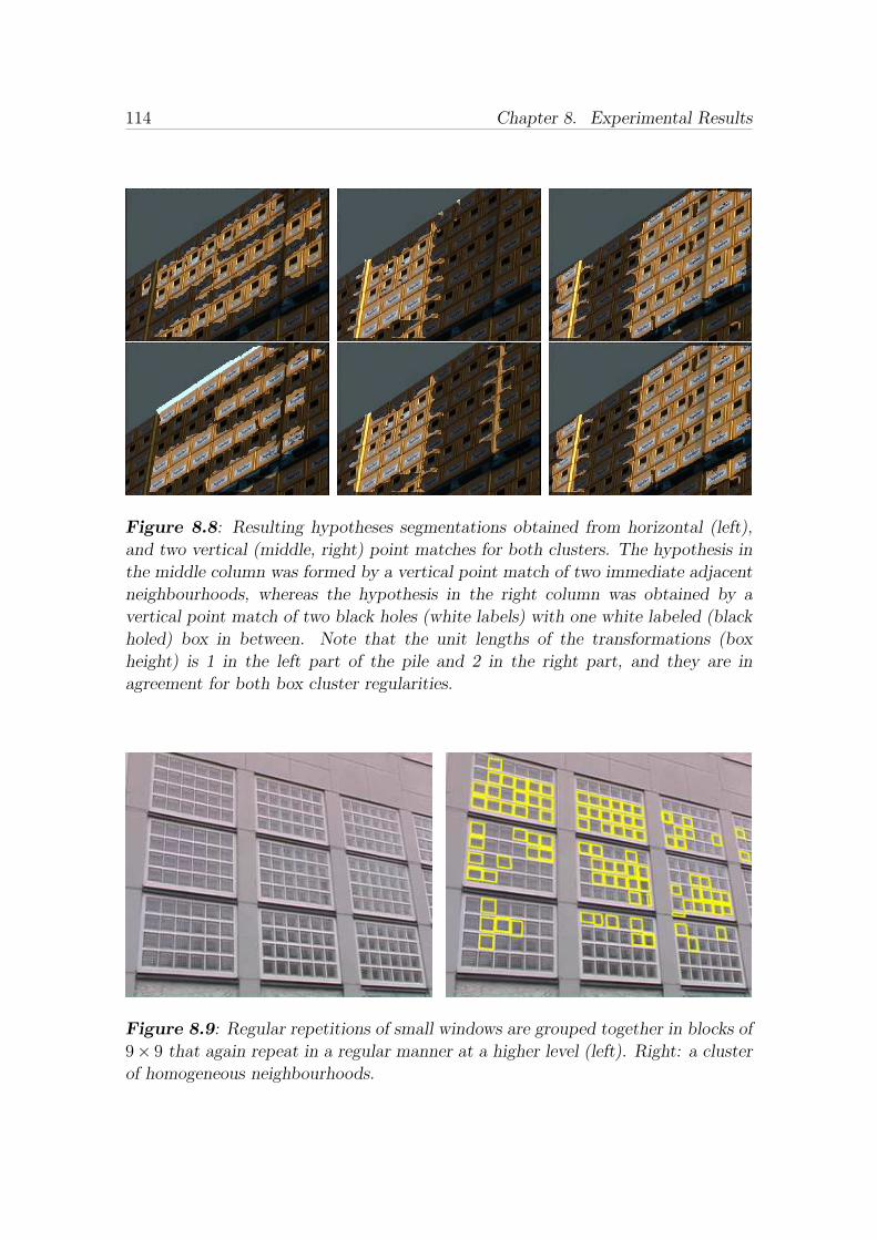
114 Chapter 8. Experimental Results
Figure 8.8: Resulting hypotheses segmentations obtained from horizontal (left),
and two vertical (middle, right) point matches for both clusters. The hypothesis in
the middle column was formed by a vertical point match of two immediate adjacent
neighbourhoods, whereas the hypothesis in the right column was obtained by a
vertical point match of two black holes (white labels) with one white labeled (black
holed) box in between. Note that the unit lengths of the transformations (box
height) is 1 in the left part of the pile and 2 in the right part, and they are in
agreement for both box cluster regularities.
Figure 8.9: Regular repetitions of small windows are grouped together in blocks of
9× 9 that again repeat in a regular manner at a higher level (left). Right: a cluster
of homogeneous neighbourhoods.

8.3. Elations 115
Figure 8.10: The presence of a high degree of symmetry becomes apparent as
the large window blocks are in agreement with elations in vertical (left), horizontal
(middle) and diagonal directions (right).
merged in larger segmentations for some directions.
Obviously, the arrangements of the window blocks are again in a regular manner.
Indeed, there is a hierarchy of groupings at two scales. At this point, the natural
question arises about how a system can detect this additional regularity at the
larger scale. Clearly, both the small scale groupings (repetitions of the windows)
and the large scale grouping (repetitions of the window blocks) share the same fixed
structures.
For such highly symmetric structures, one possi-
Figure 8.11: Visualization of
the symmetry density.
bility for the delineation of the large scale group-
ing exploits the concept of symmetry density.
In particular, the segmented areas of different
valid homology hypotheses are accumulated in
a buffer. Those areas with the largest values ex-
hibit the highest degree of symmetry. The visu-
alization of the symmetry density for the build-
ing example is shown in Figure 8.11, where the
window blocks become apparent as regions with
the highest degree of symmetry. Although no
such system has been developed yet, a symme-
try density image might serve as a good starting
point. Future work will therefore deal with a more systematic exploitation thereof,
hopefully leading to a comprehensive framework for the detection of hierarchical
groupings.
The next example deals with more complicated symmetries in the same vein. Fig-
ure 8.12 (left) shows the original situation. Here we have two principal translational
symmetries in horizontal and vertical directions that make up the regularity of the
plugs. From a geometrical viewpoint, these are two elations sharing a common van-
ishing line. More precisely, the translations in the vertical direction even share both

116 Chapter 8. Experimental Results
Figure 8.12: Symmetric arrangements of plugs with different elations that all
have the vanishing line in common. Top left: Original image. Top right: Resulting
segmentation for the horizontal direction and the vertical ones (bottom row)
fixed structures, but differ in the value of the cross-ratio. The system was able to ex-
tract the fixed structures, and the resulting segmentations are shown in Figure 8.12
for the horizontal (top right) and vertical directions (lower row). The left picture
in the bottom row shows the validation for a hypothesis that maps the upper two
rows of plugs onto each other, while the right picture illustrates the resulting seg-
mentation for the lower two rows. Note that the group of plugs of the second row
(from above) is actually in agreement with this hypothesis, and this was correctly
segmented by the system.
8.4 Conclusion
Experiments were conducted to demonstrate the overall capability of the system
to deal with symmetries related by planar homologies in a wide variety of different
8.4. Conclusion 117
images. All images were taken using regular digital cameras, and correction against
radial distortion was made where necessary. Generally speaking, the system works
reasonably well and is able to detect groupings where the repeating patterns consist
of a rich diversity of textures. This is in contrast to previous contributions that
focused on only one type of grouping and / or exploited only a narrow range of
features.
One shortcoming is the limited robustness to changes in scale during the detection of
repetitions, which is especially the case for the geometry-based invariant neighbour-
hoods. At the time this report is written, experiments are carried out to improve
the extraction of affinely invariant neighbourhoods with respect to changes in scale.
From these experiments, we can also conclude that our approach is efficient: the
average computation time required — from the extraction of interest points till hy-
potheses validation in cluttered scenes — is in the magnitude of several minutes.
This emphasizes the superiority of our strategy over traditional, combinatorial meth-
ods.


9Conclusion
Grouping in its many flavors has attracted the interest of researchers since
the early days of computer vision. The rakish definition of grouping as
’putting together what belongs together’ arose with the ongoing devel-
opment of vision systems, with a trend to increasing complexity. Yet
regardless of their complexity, many systems rely on grouping as a necessary prepro-
cessing step, where it is mostly performed at the lowest level, e.g. the organization
of edgels and lines. This explains why grouping on the lowest level is still of interest
even in present days.
It is only in recent years that attention has turned towards the detection of groupings
at a higher level in ordinary images, without the need for (manual) preprocessing
or presegmentation. These newer contributions mostly focus on regular repetitions,
and regularity implies a quantitative description that is formalized by the laws of ge-
ometry, especially projective geometry. And this is the point where the framework
developed during this dissertation enters the scene. In the following, Section 9.1
briefly recapitulates our contributions and revisits the technologies employed in the
framework. Section 9.2 finishes this report with ideas and suggestions for improve-
ments and further research.
9.1 Summary
The most similar work to ours is the grouping system by Schaffalitzky and Zisserman[Schaffalitzky and Zisserman 2000, Schaffalitzky and Zisserman 1998]. The authors
also attack the problem of finding regular repetitions in images, although their
system is limited to the case of elations. It would be mistaken to consider their
work as a starting point for this dissertation, since the strategy, techniques and
generality of our approach is completely different.
Our main contributions to intra-image grouping are manifold. First of all, our
system is able to detect regular pattern repetitions related by the more general class
119

120 Chapter 9. Conclusion
of planar homologies, which includes periodicities, mirror-symmetries and reflection
about points. This is in contrast to earlier work that focused on one particular
grouping type only. We have also shown that grouping can be performed efficiently
by banning heavy combinatorics from all processing steps. Efficiency is a crucial
issue when it comes to grouping, and here lies the novelty of our approach. Most
other systems are virtually characterized by the excessive combinatorial techniques
that they apply. Finally, our framework is more generic in the repeating features
that it is able to detect (affinely invariant neighbourhoods); most earlier approaches
are very limited in this respect.
The grouping strategy developed during this dissertation is based on the geometric
concept of fixed structures of planar homologies that relate repeating patterns in
the image. Fixed structures are geometric entities, like points and lines, that remain
fixed under a certain group of transformations. Regardless of their rather abstract
nature, fixed structures might indeed correspond to visible features in images, like for
instance a horizon line. The reason why fixed structures are of special interest is that
they lift many degrees of freedom of the transformation sought. If fixed structures
are known, the problem of finding a general 5 dof planar homology is reduced to
lifting only a single dof, which is a substantial reduction in complexity. To arrive at
candidates for fixed structures, we first detect repetitions of small, planar patches.
A second step analyzes these repetitions for their regularity, yielding fixed structures
as output.
Points of interest serve as starting points for the delineation of affinely invariant
neighbourhoods in the image. These are small, local, planar patches that self-
adapt to the underlying intensity profile, and the extraction process is invariant
against affine geometric and linear photometric changes. Each such neighbourhood
is described by a feature vector of moment invariants (color-ratios, resp.), which
allows to find neighbourhoods that cover similar patterns (i.e. repetitions) efficiently.
Several neighbourhood extraction methods are used (geometry-based / intensity-
based), and — depending on the image content — some extraction methods have
a better response than others. The idea is to have an opportunistic system that
exploits what is on offer in a specific image, such that enough affinely invariant
neighbourhoods can be extracted to get the grouping process started.
Once clusters of affinely invariant neighbourhoods have been extracted, these are
analyzed for their regularity (in a non-combinatorial way again) using a cascaded
version of the Hough transform (CHT). A line parameterization that is symmetric in
both (a, b) and (x, y) enables the iterated application of the Hough transform, where
the output of a previous transform can be used as input for a subsequent one. The
CHT yields fixed structure candidates (if any), and a single neighbourhood-match
suffices to lift the remaining dof and hence to arrive at the long awaited planar
homology hypothesis. Each hypothesis is then validated for its correctness, which
results in a segmentation of the image into symmetric parts.

9.2. Discussion and Outlook 121
9.2 Discussion and Outlook
9.2.1 Improvements
The proposed framework can still be improved in a number of ways. This holds
especially for a comprehensive system like ours that is a synthesis of methods and
knowhow from rather diverse corners of Computer Vision. Each method has its own
specific advantages and shortcomings, and improvements to each of them pay off to
the overall effectiveness and robustness of the entire grouping system.
First of all, the extraction of affinely invariant neighbourhoods is a self-contained,
complex system with plenty of room for optimization. Many suggestions for im-
provements were already pointed out by Tuytelaars ([Tuytelaars 2000]). Some of
them have been realized during this thesis, so for instance a more efficient coding
and thus speed improvements towards almost real-time (for some neighbourhood
types). However, one shortcoming is the lack of robustness against major changes
in scale. Experiments have already been made to render the neighbourhood extrac-
tion more stable in this respect, with promising results. Further work will therefore
incorporate these extensions.
Another problem is the increasing number of parameters as more functionality is
added to the system. As mentioned earlier, the values for the 57 most important
parameters have been found empirically based on a diversity of test images. For cases
where the system fails to find groupings using the set of default values, a detection
can nevertheless be enforced by tuning the parameters accordingly. However, this
runs against the goal of an automated system. We have not paid much attention yet
to the determination of parameter values in an adaptive, data-driven or smart way.
As many parameters are geometry-specific, an additional processing stage could be
inserted between low-level feature extraction and the extraction of affinely invariant
neighbourhoods. The collection of statistics about geometric primitives (such as the
median of edge lengths etc.) would be the purpose of this stage, which would adapt
the following neighbourhood extraction stage to the realities in the image.
In the same spirit, an automatic parameter-adaption would improve the cascaded
Hough transform as well. The question is whether the coarseness of quantization
of Hough spaces can be set adaptively based on the geometric structures in the
image and the desired accuracy. Although one might argue that CPU and memory
requirements are no longer a problem nowadays (remember Moore’s law), filter-
ing operations still pose a computational burden that can certainly be lowered by
avoiding unnecessary accumulator sizes.
Also interesting is a more systematic exploit of color information, and this is ar-
guably a notoriously difficult task and still an open field of research. Is it possible to
obtain a higher discriminative power of features by choosing a different color space,

122 Chapter 9. Conclusion
such that invariance against linear photometric changes is preserved ? For instance,
homogeneous affinely invariant neighbourhoods might clearly benefit from this im-
provement, as the metrics in the currently used RGB color space is not always
in agreement in what a human observer perceives. Similarity measures based on
normalized cross-correlation of graylevel values are pervasive throughout the entire
grouping system. Can correlation be made more effective by including the spec-
tral information in a more appropriate way ? Reports on generalized correlation
can be found in [Jawahar and Narayanan 2002] and might indeed help in a better
discrimination of features.
9.2.2 Future Work
After being able to deal with groupings related by planar homologies, it is natural
to ask for extensions towards other types symmetries, in particular rotational sym-
metries. To this date, only a few authors have tackled the problem of recognition of
rotational symmetries ([Forsyth et al. 1992]), or have shown that 3D objects with fi-
nite rotational symmetry induce geometric relations in the image ([Liu et al. 1995]).
However, no automatic system has been reported yet. Here, it is desirable to extend
the concept of fixed structures for rotational symmetries, to be nicely integrated in
the existing framework. For repeating patterns in a rotation-symmetric configura-
tion, the fixed structures correspond to pencils of conics, and these require more
than two parameters for their specification. How they can be extracted efficiently
is subject to ongoing research.
Apart from rotational symmetries, the systematic analysis of interrelations between
different groupings in the same image poses a further challenge. Examples shown
earlier have already led us to this problem, and common fixed structures are al-
ready a good indication for hidden relations. Clearly, these are all non-accidental
arrangements. Our observations have shown that the segmented regions (hypothe-
sis validations) might play an important role: Different groupings (with or without
common fixed structures) might have different (isolated) or overlapping segmen-
tations. Those areas in the image with overlapping segmentations are of special
interest, as they indicate a ’higher degree’ of symmetry. In this context, it would be
interesting to establish a link to wallpaper groups, although we only face truncated
versions thereof in images. Nevertheless, an analysis for wallpaper regularities is
possible by moving the fixed structures to infinity, thereby removing perspective
distortions. In this respect, the work by Liu and Collins ([Liu and Collins 2001,
Liu and Collins 2000]) complements our work very well in that our system is able
to delineate regions of high symmetry automatically (the system by Liu and Collins
requires manual selection of symmetric image parts).
Alternatively, a more elaborate theoretical treatment might solely be based fixed
structures. Analyzing them would allow to infer information about missing fixed

9.2. Discussion and Outlook 123
structures that went undetected by the CHT. It can indeed be shown that, for
three planar homologies in a triangular configuration, a classifactory structure can
be derived. Encouraging preliminary experiments have already been made in this
respect ([Tuytelaars et al. 2002]).
Finally, groupings may occur at different hierarchical levels. For instance, each half
of a mirror-symmetry might contain some regularity itself. Or think at the building
facade with repeating windows shown in Figure 8.9 in Chapter 8. Such groupings
need also to be found. To that end, the concept of the symmetry density image has
already coarsely delineated the window blocks, and principally the CHT might again
be applied to e.g. the center of gravities of these regions of high symmetry to detect
the grouping at the larger scale. Concepts and strategies for the integration of these
extensions still have to be determined, and this will be the focus of future work,
which clearly emphasizes the yet undiscovered potential of this strand of research.


ALinear Discriminant Analysis
One of the recurring problems encountered in applying statistical techniques to
pattern recognition problems is the reduction of dimensionality. Procedures that are
analytically or computationally manageable in low-dimensional spaces can become
completely impractical in high-dimensional spaces. Thus, various techniques have
been developed for reducing the dimensionality of the feature space in the hope of
obtaining a more manageable problem.
The dimensionality can be reduced from d dimensions to one dimension if the d
dimensional data is merely projected onto a line. Of course, even if the samples
form well-separated, compact clusters in d-space, projection onto an arbitrary line
will usually produce a confused mixture of samples from all of the classes. However,
by moving the line around, an orientation might be found for which the projected
samples are well separated. And this is exactly the goal we wish to achieve here
for the more general case, that is the reduction of dimensionality from d to k with
k < d.
A.1 Principle
We illustrate the linear discriminant analysis as applied in this dissertation with an
artificial example. Figure A.1 shows three well-separated clusters in 2D. The specific
nature of the features plotted here is not of interest at the moment. The different
number of data-points in each cluster were randomly drawn from four bivariate
normal distributions that differ only in the mean. Important here is that all clusters
have approximately the same spread, which is according to the common covariance
matrix assumption.
Finding a projection line for which the samples are still well separated after pro-
jection is quite straightforward for the configuration in Figure A.1. The x-axis is
obviously the best choice. However, the task gets more difficult when the feature
125

126 Appendix A. Linear Discriminant Analysis
-2 -1 1 2 3 4
-5
5
10
Figure A.1: Initial cluster configuration.
space exceeds three dimensions and the projection line or plane (or subspace) must
be found automatically.
The first step is a rotation of the coordinate frame in the direction of the largest
(cluster-specific) spread, followed by whitening of the data. Whitening is a rescaling
of the axes, resulting in ’sphere’-like clusters. The effect of this step can be seen in
Figure A.2. Although hardly visible, the clusters are now sphere-like, i.e. the vari-
-2 -1 1 2
-20
-10
10
20
30
40
Figure A.2: Transformed dataset after rotation and scaling.
ances of each cluster are now normalized in both dimensions in this new coordinate
frame. From a computational viewpoint, the transformation is performed based on
the singular value decomposition of the cluster-specific covariance matrix ΣC:
ΣC = U ·D ·V> (A.1)

A.2. Covariance Matrix Based on Tracking Experiments 127
with U and V orthogonal and D diagonal. The entries Dii on the diagonal are the
variances, sorted in ascending order.
Note the increase of the inter-cluster distance in this particular example. This is
due to the fact that the standard deviation of the first component (w.r.t the original
coordinate frame in Figure A.1) is smaller than one. The net effect is a compression
in one direction with a dilution for the other one, which results in larger distances
between the clusters for this particular configuration.
Next, a rotation is applied to the transformed dataset, but this time based on the
singular value decomposition of the global covariance matrix ΣG of the transformed
data. Roughly speaking, the global covariance matrix takes into account the overall
variability of the clusters. Applied to the example shown here, this results again
in a 90 degree rotation, as shown in Figure A.3. Actually, this second transform
-20 -10 10 20 30 40
-2
-1
1
2
Figure A.3: Situation after the second transform.
corresponds to a principal component analysis. In general, a reduction of the dimen-
sionality can now be obtained by projection onto the first few principal components
(the x-axis in Figure A.3), thereby keeping the different clusters well separated.
A.2 Covariance Matrix Based on Tracking Exper-
iments
In the following, the term feature refers to the feature vector of an affinely invariant
neighbourhood. Simply speaking, we want to arrive at an estimate for a feature-
specific covariance matrix that represents the overall variability of a feature to the
best possible extent. Remember that different neighbourhood types have different

128 Appendix A. Linear Discriminant Analysis
feature spaces, hence each neighbourhood type has its own specific covariance matrix
Σ.
We obtained estimates Σ by tracking invariant neighbourhoods throughout a video
sequence: In the first frame, three affinely invariant neighbourhoods covering differ-
ent parts on the physical surface of an object were manually identified. Next, the
camera was gradually moved and the illumination slightly changed. This way, the
scene is imaged from different viewpoints (under varying illumination conditions)
and the three appointed neighbourhoods were manually identified in the consecutive
frames.
For each cluster, the mean was determined and subtracted from all feature vectors
belonging to that cluster. This allows to look at the deviations only. Then, all
clusters were put together again to compute the covariance matrix. This yields an
estimate of the covariance matrix based on the average of some clusters.
Of course, this is only a rudimentary estimate, since so many factors account for the
overall variability (see Section 6.3.1) that can never by fully covered by a tracking
experiment. Nevertheless, given the same dataset used in the tracking experiment,
we determined the average separability of the clusters using both the pooled and
feature-specific covariance matrix. Table A.1 confirms that the ratio of inter to intra-
cluster distances is remarkably larger when using a LDA. The results are shown in
Cluster 1 2 3
1 0 4.3554 4.193
2 4.3554 0 4.2047
3 4.193 4.2047 0
Cluster Intra-cluster distance
1 3.8594
2 3.9993
3 3.1486
Cluster 1 2 3
1 0 23.90 29.33
2 23.90 0 26.13
3 29.33 26.13 0
Cluster Intra-cluster distance
1 4.4317
2 4.2403
3 3.7756
Table A.1: Inter- (left column) and intra (right column) cluster distances obtained
using a global covariance matrix estimate (top row) and the covariance matrix based
on tracking experiments (bottom row).
Table A.1. The distances shown are actually the averaged distances between all the
feature vectors of different clusters and within the same cluster.

BImage Database Overview
Figure B.1: Example images the system was applied to.
129

130 Appendix B. Image Database Overview
Figure B.2: Example images the system was applied to (ctd.)
Bibliography
[Barnard 1983] S. Barnard. Interpreting perspective images. Artificial Intelligence,
21:435–462, 1983.
[Baumberg 2000] A. Baumberg. Reliable feature matching across widely separated
views. In IEEE Computer Society Conference on Computer Vision and Pattern
Recognition, pages 774–781. IEEE, 2000.
[Binford 1981] T. Binford. Inferring Surfaces from Images. Artificial Intelligence,
17:205–244, 1981.
[Bruckstein and Shaked 1998] A.M. Bruckstein and D. Shaked. Skew-Symmetry
Detection via Invariant Signatures. Pattern Recognition, 31(2):181–192, 1998.
[Canny 1986] J. Canny. A computational approach to edge detection. IEEE Trans-
actions on Pattern Analysis and Machine Intelligence, 8:679–698, 1986.
[Cham and Cipolla 1996] T. Cham and R. Cipolla. Geometric Saliency of Curve
Correspondences and Grouping of Symmetric Contours. In European Confer-
ence on Computer Vision, volume 1, pages 385–398, Cambridge, UK, April 1996.
Springer.
[Duda and Hart 1972] R.O. Duda and P.E. Hart. Use of the hough transform to
detect lines and curves in pictures. 15:11–15, 1972.
[Ferrari et al. 2001] V. Ferrari, T. Tuytelaars, and L. Van Gool. Markerless aug-
mented reality with a real-time affine region tracker. In Procs. of the IEEE and
ACM Intl. Symposium on Augmented Reality, 2001.
[Fischler and Bolles 1981] M. A. Fischler and R.C. Bolles. Random sample con-
sensus: A paradigm for model fitting with applications to image analysis and
automated cartography. Communications of the ACM, 24(6):381–395, 1981.
[Forsyth et al. 1992] D.A. Forsyth, J. Mundy, A. Zisserman, and C.A. Rothwell.
Recognising rotationally symmetric surfaces from their outlines. In European
Conference on Computer Vision, pages 639–647, 1992.
[Friedberg 1986] S. A. Friedberg. Finding Axes of Skewed Symmetry. Computer
Vision, Graphics, and Image Processing, 34:138–155, 1986.
131

132 Bibliography
[Friedman 1989] J. Friedman. Regularized discriminant analysis. Journal of the
American Statistical Association, 84(405):165–175, March 1989.
[Gallagher 2002] A.C. Gallagher. A ground truth based vanishing point detection
algorithm. Pattern Recognition, 35:1527–1543, 2002.
[Glachet et al. 1993] R. Glachet, J.T. Lapreste, and M. Dhome. Locating and Mod-
elling a Flat Symmetric Object from a Single Perspective Image. Computer
Vision, Graphics, and Image Processing: Image Understanding, 57(2):219–226,
March 1993.
[Gross and Boult 1991] A. Gross and T. Boult. SYMAN: A SYMetry ANalyzer. In
IEEE Computer Society Conference on Computer Vision and Pattern Recognition,
pages 744–746. IEEE, 1991.
[Gross and Boult 1994] A. Gross and T. Boult. Analyzing skewed symmetries. In-
ternational Journal of Computer Vision, 13(1):91–111, 1994.
[Harris and Stephens 1988] C. Harris and M. Stephens. A combined corner and edge
detector. In Proc. Jth Alvey Vision Conf., pages 147–151, 1988.
[Hartley and Zisserman 2000] R. Hartley and A. Zisserman. Multiple View Geome-
try in Computer Vision. Cambridge University Press, 2 edition, 2000.
[Huttenlocher and Wayner 1992] D. Huttenlocher and P. Wayner. Finding Convex
Edge Groupings in an Image. International Journal of Computer Vision, 8(1):7–
27, 1992.
[Illingworth and Kittler 1988] J. Illingworth and J. Kittler. A survey of the hough
transform. Computer Vision, Graphics, and Image Processing, 44:87–116, 1988.
[Jacobs 1989] D. Jacobs. Groups for recognition. MIT AI Memo 1177, 1989.
[Jacobs 1996] D. Jacobs. Robust and efficient detection of salient convex groups.
IEEE Transactions on Pattern Analysis and Machine Intelligence, 1(18), 1996.
[Jawahar and Narayanan 2002] C.V. Jawahar and P.J. Narayanan. Generalised cor-
relation for multi-feature correspondence. Pattern Recognition, 35:1303–1313,
2002.
[Kanade 1981] T. Kanade. Recovery of the Three-Dimensional Shape of an Object
from a Single View. Artificial Intelligence, 17:409–460, 1981.
[Leavers 1993] V. F. Leavers. Which hough transform ? Computer Vision, Graph-
ics, and Image Processing, 58(2):250–264, 1993.
[Leung and Malik 1996] T. Leung and J. Malik. Detecting, localizing and grouping
repeated scene elements from an image. In European Conference on Computer
Vision, volume 1, pages 546–555, England, April 1996.
[Lin et al. 1997] H.-C. Lin, L.-L. Wang, and S.-N. Yang. Extracting periodicity of a
regular texture based on autocorrelation functions. Pattern Recognition Letters,
18:433–443, 1997.
Bibliography 133
[Liu and Collins 2000] J. Liu and T. Collins. A Computational Model for Repeated
Pattern Perception using Frieze and Wallpaper Groups. In IEEE Computer So-
ciety Conference on Computer Vision and Pattern Recognition, 2000.
[Liu and Collins 2001] J. Liu and T. Collins. Skewed Symmetry Groups. In IEEE
Computer Society Conference on Computer Vision and Pattern Recognition, De-
cember 2001.
[Liu et al. 1995] J. Liu, J. Mundy, and A. Zisserman. Grouping and structure re-
covery for images of objects with finite rotational symmetry. In Proc. Asian
Conference on Computer Vision, volume 1, pages 379–382, 1995.
[Lowe 1985] D. Lowe. Perceptual Organization in Visual Recognition. Kluwer Aca-
demic Publishers, 1985.
[Lutton et al. 1994] E. Lutton, H. Maıtre, and J. Lopez-Krahe. Contribution to the
determination of vanishing points using hough transform. IEEE Transactions on
Pattern Analysis and Machine Intelligence, 16(4), 1994.
[Matas et al. 2002] J. Matas, S. Obdrzalek, and O. Chum. Local affine frames for
wide-baseline stereo. In International Conference on Pattern Recognition, August
2002.
[Mindru et al. 1998] F. Mindru, T. Moons, and L. Van Gool. Color-based moment
invariants for viewpoint and illumination independent recognition of planar color
patterns. In Intl. Conf. on Advances in Pattern Recognition, pages 113–122, 1998.
[Mindru et al. 1999a] F. Mindru, T. Moons, and L. Van Gool. Recognizing color
patterns irrespective of viewpoint and illumination. In IEEE Computer Society
Conference on Computer Vision and Pattern Recognition, volume 1, pages 368–
373, 1999.
[Mindru et al. 1999b] F. Mindru, T. Moons, and L. Van Gool. Recognizing color
patterns irrespective of viewpoint and illumination. In IEEE Computer Society
Conference on Computer Vision and Pattern Recognition, pages 368–373, 1999.
[Mindru et al. 2001] F. Mindru, T. Moons, and L. Van Gool. The influence of in-
tensity transformation models on illumination and viewpoint independent color
pattern recognition. In IEEE Computer Society Conference on Computer Vision
and Pattern Recognition, December 2001. Post-Conference workshop on Identify-
ing Objects Across Variations in Lighting: Psychophysics and Computation.
[Mukherjee et al. 1995] D. P. Mukherjee, A. Zisserman, and M. Brady. Shape from
Symmetry – Detecting and Exploiting Symmetry in Affine Images. In Phil. Trans.
R. Soc. Lond. A, pages 77–106. 1995.
[Oren and Nayar 1994] M. Oren and S. Nayar. Seeing beyond lamberts law. In
European Conference on Computer Vision, pages 269–280, 1994.

134 Bibliography
[Pauwels and Frederix 1999] E. Pauwels and G. Frederix. Finding salient regions
in images: Non-parametric clustering for image segmentation and grouping. 75,
Jul./Aug. 1999.
[Ponce 1988] J. Ponce. Ribbons, symmetries and skewed symmetries. In ARPA Im-
age Understanding Workshop, volume 2, pages 1074–1079, Massachusetts, 1988.
[Reiss 1993] T. Reiss. Recognizing planar objects using invariant image features.
LNCS. Springer, 1993.
[Richards and Jepson 1992] W. Richards and A. Jepson. What Makes a Good Fea-
ture ? MIT AI Memo 1356, 1992.
[Roche et al. 1999] A. Roche, G. Malandain, and N. Ayache. Unifying maximum
likelihood approaches in medical image registration. Technical Report 3741, IN-
RIA, 1999.
[Schaffalitzky and Zisserman 1998] F. Schaffalitzky and A. Zisserman. Geometric
grouping of repeated elements within images. In Proc. 9’th British Machine Vision
Conference, pages 13–22, Southampton, 1998.
[Schaffalitzky and Zisserman 2000] F. Schaffalitzky and A. Zisserman. Planar
grouping for automatic detection of vanishing lines and points. Image and Vision
Computing, 18(9):647–658, June 2000.
[Schmid and Mohr 1997] C. Schmid and R. Mohr. Local greyvalue invariants for
image retrieval. IEEE Transactions on Pattern Analysis and Machine Intelligence,
19(6):872–877, may 1997.
[Schmid et al. 2000] C. Schmid, R. Mohr, and C. Bauckhage. Evaluation of interest
point detectors. International Journal of Computer Vision, 37(2):151–172, 2000.
[Scott 1992] D.W. Scott. Multivariate Density Estimation. John Wiley & Sons,
1992.
[Semple and Kneebone 1952] J.G. Semple and G.T. Kneebone. Algebraic Projective
Geometry. Oxford University Press, 1952.
[Sha’ashua and Ullman 1988] A. Sha’ashua and S. Ullman. Structural Saliency:
The Detection of Globally Salient Structures Using a Locally Connected Network.
In Intl. Conf. on Computer Vision, pages 321–327, 1988.
[Springer 1964] C. Springer. Geometry and Analysis of Projective Spaces. Freeman,
1964.
[Turina et al. 2001a] A. Turina, T. Tuytelaars, and L. Van Gool. Efficient grouping
under perspective skew. In IEEE Computer Society Conference on Computer Vi-
sion and Pattern Recognition, volume 1, pages 247–254, Kauai, Hawaii, December
2001. IEEE Computer Society.
[Turina et al. 2001b] A. Turina, T. Tuytelaars, T.Moons, and L. Van Gool. Group-
ing via the matching of repeated patterns. In S. Singh, N. Murshed, and
Bibliography 135
W. Kropatsch, editors, Intl. Conf. on Advances in Pattern Recognition, number
2013 in Lecture Notes in Computer Science, pages 250–259, March 2001.
[Tuytelaars and Van Gool 1999] T. Tuytelaars and L. Van Gool. Content-based
image retrieval based on local, affinely invariant regions. In Proc. Third Intl.
Conf. on Visual Information Systems, pages 493–500, 1999.
[Tuytelaars and Van Gool 2000] T. Tuytelaars and L. Van Gool. Wide baseline
stereo based on local, affinely invariant regions. In Proc. British Machine Vision
Conf., pages 412–422, 2000.
[Tuytelaars et al. 1998a] T. Tuytelaars, L. Van Gool, M. Proesmans, and T. Moons.
The cascaded hough transform as an aid in aerial image interpretation. In Intl.
Conf. on Computer Vision, pages 67–72, January 1998.
[Tuytelaars et al. 1998b] T. Tuytelaars, L. Van Gool, M. Proesmans, and T. Moons.
A cascaded hough transform as an aid in aerial image interpretation. In Intl. Conf.
on Computer Vision, pages 67–72, 1998.
[Tuytelaars et al. 2002] T. Tuytelaars, A. Turina, and L. Van Gool. Non-
combinatorial detection of regular repetitions under perspective skew. Accepted
for IEEE Transactions on Pattern Analysis and Machine Intelligence, 2002.
[Tuytelaars 2000] T. Tuytelaars. Local, invariant features for registration and recog-
nition. PhD thesis, Katholieke Universiteit Leuven, December 2000.
[Van Gool and Proesmans 1995] L. Van Gool and M. Proesmans. Grouping and
Invariants using Planar Homologies. In R. Mohr and W. Chengke, editors, Europe-
China Workshop on Geometrical Modelling and Invariants for Computer Vision,
pages 182–189. Xidan University Press, Xi’an, 1995.
[Van Gool et al. 1994] L. Van Gool, T. Moons, and M. Proesmans. Groups,
fixed sets, symmetries and invariants. Technical report, KUL/ESAT/MI2/9426,
Katholieke Universiteit Leuven, 1994.
[Van Gool et al. 1995a] L. Van Gool, T. Moons, and M. Proesmans. Groups for
grouping: a strategy for the exploitation of geometrical constraints. In Proc. 6th
Int. Conf. on Computer Analysis of Images and Patterns, pages 1–8, Prague,
Czechia, 1995.
[Van Gool et al. 1995b] L. Van Gool, T. Moons, D. Ungureanu, and A. Oosterlinck.
The Characterization and Detection of Skewed Symmetries. Computer Vision
and Image Understanding, 61(1):138–195, 1995.
[Van Gool et al. 1995c] L. Van Gool, T. Moons, D. Ungureanu, and E. Pauwels.
Symmetry from Shape and Shape from Symmetry. Int. J. of Robotics Research,
14(5):407–424, 1995.
[Van Gool et al. 1996] L. Van Gool, T. Moons, and D. Ungureanu. Geomet-
ric/photometric invariants for planar intensity patterns. In European Conference

136 Bibliography
on Computer Vision, volume 1 of Lecture Notes in Computer Science, pages 642–
651, Cambridge, UK, April 1996. Springer.
[Van Gool et al. 1998] L. Van Gool, M. Proesmans, and A. Zisserman. Planar Ho-
mologies as a basis for Grouping and Recognition. Image and Vision Computing,
16(1):21–26, 1998.
[Van Gool et al. 2001] L. Van Gool, T. Tuytelaars, and A. Turina. Local features
for image retrieval. In R. C. Veltkamp, H. Burkhardt, and H-P. Kriegel, edi-
tors, State-of-the-Art in Content-Based Image and Video Retrieval, volume 22 of
Computational Imaging and Vision, pages 21–41. Kluwer Academic Publishers,
2001.
[Van Gool 1997] L. Van Gool. A Systematic Approach to Geometry-Based Group-
ing and Non-accidentalness. In G. Sommer and J. Koenderink, editors, Alge-
braic Frames for the Perception-Action Cycle (AFPAC’97), volume 1315 of Lec-
ture Notes in Computer Science, pages 126–147, Kiel, Germany, September 1997.
Springer.
[Van Gool 1998] L. Van Gool. Projective subgroups for grouping. Phil. Trans. R.
Soc. Lond. A, 356(1740):1251–1266, 1998.
[Viola and Wells 1997] P. Viola and W. Wells. Alignment by maximization of mu-
tual information. International Journal of Computer Vision, 24(2):137–154, 1997.
[Wertheimer 1923] M. Wertheimer. Untersuchungen zur Lehre von der Gestalt II.
Psychol. Forschung, 4:301–350, 1923.
[Witkin and Tennenbaum 1983] A. Witkin and J. Tennenbaum. On the Role of
Structure in Vision. In J. Beck, B. Hope, and A. Rosenfeld, editors, Human and
Machine Vision. Academic Press, New York, 1983.
[Wolff 1994] L. Wolff. On the relative brightness of specular and diffuse reflection.
In European Conference on Computer Vision, pages 369–376, 1994.
[Xu 1988] L. Xu. A method for recognizing configurations consisting of line sets
and its application to discrimination of seismic face structures. In International
Conference on Pattern Recognition, pages 610–612, 1988.

Curriculum Vitae
Andreas Turina
Date of birth: 4th of June, 1971
Place of birth: Zurich, Switzerland
Citizenship: Fallanden, ZH
Education: 1978–1984 Primary School in Pfaffhausen (ZH).
1984–1989 High School, Matura Type B (Realgymna-
sium Ramibuhl, Zurich).
1990–1992 Studies of Physics at the Swiss Federal In-
stitute of Technology Zurich.
1993–1999 Studies of Electrical Engineering at the
Swiss Federal Institute of Technology
Zurich. Graduation with the degree
Dipl. El.-Ing. ETH.
1992, 1993
1996
Initial military service and officers’ school
at the Swiss Air Force.
1999–2002 Doctoral student at the Swiss Federal In-
stitute of Technology (ETH) Zurich.
Occupations: 1992–1993 Zurich State Police, Airport Division.
1997 Internship at Sulzer Carbomedics, Austin
TX.
1999–2002 Research assistant at ETH Zurich, Com-
puter Vision Group.